link at the published version:
TRANSCRIPT
This item was downloaded from IRIS Università di Bologna (https://cris.unibo.it/)
When citing, please refer to the published version.
“This is a post-peer-review, pre-copyedit version of an article published in “Mathematical Programming”. The final authenticated version is available online at:
https://doi.org/10.1007/s10107-018-1243-y ” Link at the published version: https://link.springer.com/article/10.1007/s10107-018-1243-y
© 2018 Springer-Verlag
Rights / License:
The terms and conditions for the reuse of this version of the manuscript are specified in the publishing policy. For all terms of use and more information see the publisher's website.

Noname manuscript No.(will be inserted by the editor)
Routing Optimization with Time Windows under
Uncertainty
Yu Zhang · Roberto Baldacci · MelvynSim · Jiafu Tang
Received: date / Accepted: date
Abstract We study an a priori Traveling Salesman Problem with Time Win-dows (tsptw) in which the travel times along the arcs are uncertain and thegoal is to determine within a budget constraint, a route for the service vehiclein order to arrive at the customers’ locations within their stipulated time win-dows as well as possible. In particular, service at customer’s location cannotcommence before the beginning of the time window and any arrival after theend of the time window is considered late and constitutes to poor customerservice. In articulating the service level of the tsptw under uncertainty, wepropose a new decision criterion, called the essential riskiness index, which hasthe computationally attractive feature of convexity that enables us to formu-late and solve the problem more effectively. As a decision criterion for articu-lating service levels, it takes into account both the probability of lateness andits magnitude, and can be applied in contexts where either the distributionalinformation of the uncertain travel times is fully or partially known. We pro-
Dr. Yu ZhangDepartment of Systems Engineering, State Key Lab of Synthetic Automation of ProcessIndustries, Northeastern University, 110004 Shenyang, P.R. ChinaE-mail: [email protected]
Prof. Roberto BaldacciDepartment of Electrical, Electronic, and Information Engineering “Guglielmo Marconi”(DEI), University of Bologna, 47521 Cesena, ItalyTel.: +39-0547-339234Fax: +39-0547-339208E-mail: [email protected]
Prof. Melvyn SimDepartment of Analytics & Operations, National University of Singapore, S119245 Singa-pore, Republic of SingaporeE-mail: [email protected]
Prof. Jiafu TangCollege of Management Science and Engineering, Dongbei University of Finance and Eco-nomics, 116000 Dalian, P.R. ChinaE-mail: [email protected]
2 Yu Zhang et al.
pose a new formulation for the tsptw, where we explicitly express the servicestarting time at each customer’s location as a convex piecewise affine functionof the travel times, which would enable us to obtain the tractable formulationof the corresponding distributionally robust problem. We also show how tooptimize the essential riskiness index via Benders decomposition and presentcases where we can obtain closed-form solutions to the subproblems. We alsoillustrate in our numerical studies that this approach scales well with the num-ber of samples used for the sample average approximation. The approach canbe extended to a more general setting including Vehicle Routing Problem withTime Windows with uncertain travel times and customers’ demands.
Keywords vehicle routing problem · uncertain travel time · time windows ·risk and ambiguity · distributionally robust optimization
Mathematics Subject Classification (2000) 90C15 · 49M27 · 90C11 ·90C22
1 Introduction
In the deterministic setting, Dantzig and Ramser (1959) are first to introducethe vehicle routing problem (vrp) as an extension to the Traveling SalesmanProblem (tsp) to optimize routes for a fleet of vehicles for the purpose ofdelivering goods to or collecting them from customers at various locations.Due to its practical importance, despite the computational challenges, the vrphas received much attentions from both industry practitioners and academicresearchers (see, for instance, Laporte 2009, Toth and Vigo 2014). Amongthe variants of the vrp family, the Capacitated vrp (cvrp) and the vrp
with Time Windows (vrptw) are most prominent and have been studiedextensively (see, for instance, Baldacci et al 2012, Desaulniers et al 2014). Inthe former problem, a fleet of identical vehicles located at a central depot areoptimally routed to fulfill the demands of the customers subject to vehicularcapacity constraints. vrptw generalizes the cvrp by further imposing thateach customer has to be served within a specified time interval, known as thetime window. Specifically, if a vehicle arrives early, service cannot be rendereduntil the commencement of the time window. Furthermore, any arrival afterthe end of the time window or deadline would be prohibited. Notably, thevrp with Deadline (vrpd) is an important special case of vrptw, wherethe customers’ time windows are only specified by deadlines. When only onevehicle route is involved, we refer to the vrptw and the vrpd respectively asthe tsp with Time Windows (tsptw) and the tsp with Deadlines (tspd).
Since tsp, the simplest form of vrp, is alreadyNP-hard, incorporating un-certainty in vrp would further elevate the computational difficulties of solvingthe problem. Hence, most routing optimization problems considered in thevrp literature assume deterministic travel times. For the state-of-the-art ex-act algorithms for deterministic vrp, we refer readers to Baldacci et al (2010),Toth and Vigo (2014), Pecin et al (2017a,b), among others. Nevertheless, from

Routing Optimization with Time Windows under Uncertainty 3
the modeling perspective, ignoring uncertainty at the planning level can po-tentially result in poor routing decisions leading to, among other things, poorcustomer services that could adversely impact on the reputation of the com-pany. Hence, approaches that could mitigate uncertainty in vrp are highlydesired.
Several models and algorithms have been proposed in the literature tomitigate uncertain travel times in tspd and vrpd. Kao (1978) develops apreference ordered dynamic programming approach to address a stochastictspd that minimizes the probability of late completions. However, as notedby Sniedovich (1981), the approach may yield suboptimal solutions. Laporteet al (1992) propose a chance-constrained model (see, for instance, Charnes andCooper 1959) for a stochastic vrpd, which minimizes the operating cost whilelimiting the probability of late returns of vehicles to the depot. They presentinstances, such as having normally distributed travel times, under which thismodel can be transformed to a deterministic optimization problem. They alsopropose models that minimize the operating and expected tardiness costs,and provide a branch-and-cut procedure to solve these models via sample av-erage approximations. Kenyon and Morton (2003) propose two branch-and-cutprocedures for addressing a stochastic vrpd that minimizes the expected com-pletion time of the vehicle fleet or its tardiness probability. The first approachis capable of obtaining exact solutions when the sample size is small, whilethe second approach could obtain approximate solutions for larger probleminstances. Verweij et al (2003) provide a computational study of the decompo-sition and branch-and-cut techniques for solving a stochastic tspd via sampleaverage approximation, in which the objective is to minimize the operatingand expected tardiness costs. Tas et al (2014) propose a column generationprocedure for solving the stochastic vrptw that minimizes sum of the operat-ing costs and expected penalty costs of time window violations. Note that theenforcement of time windows in this model is “soft” in the sense that servicecommencement is permitted even if the vehicle arrives early at a customer’slocation.
The literature on stochastic vrp with “hard” time windows is rather lim-ited. The resulting optimization problem is considerably more difficult thanthe case with soft time windows, since the probability distributions of arrivaltimes at customers locations have to be truncated because of the hard timewindows. Errico et al (2016b) consider the vrp with hard time windows andstochastic service times and formulated it as a chance-constrained optimiza-tion model that includes a probabilistic constraint. The same problem hasbeen recently addressed by Errico et al (2016a) and modelled as a two-stagestochastic program using two recourse policies to recover operations feasibilitywhen the first stage plan turns out to be infeasible. The problem has beenformulated as a set partitioning problem and solved by an exact branch-cut-and-price algorithm.
A review of the literature on the stochastic vrp including stochastic de-mands, customers and travel times, and a concise description of relevant solu-tion concepts is found in Gendreau et al (2014).

4 Yu Zhang et al.
Robust optimization techniques have also been applied to address vrp
with uncertain travel times. Based on the so called budgeted uncertainty setsof Bertsimas and Sim (2003), Lee et al (2011) study a robust vrpd whichensures feasible schedules for all uncertainty arising from the uncertainty sets,while minimizing the total travel costs. Agra et al (2013) extend this approachto investigate a robust vrptw.
Our approach to address the vrptw under uncertainty is inspired by arecent work of Jaillet et al (2016), who propose a new decision criterion thatcan be applied to solve a variety of vrps under uncertainty. In particular, theymotivate and adopt a relatively new targeted oriented decision criterion thatis based on the riskiness index of Aumann and Serrano (2008) and has beengeneralized by Brown and Sim (2009) from the perspective of satisficing indecsion making. The decision criterion is a convex function that penalizes therisks of constraints’ violations by accounting for both their infeasibility prob-abilities and magnitudes of violations. Apart from the coherency in decisionmaking, the convexity of the decision criterion has important ramificationsin solving the tsp, that would lead to better performance in computationalstudies against an approach that maximizes the feasibility probability (see alsocomputational results in Adulyasak and Jaillet 2015). However, although theriskiness index can be adopted for distributionally robustness, where proba-bility distributions of the uncertain parameters are not fully characterized,to achieve computationally tractable models, it requires the uncertain out-comes to be expressed as affine summations of independently random vari-ables. Hence, while the approach can be applied to address uncertain vrp
in various settings included those with deadlines, soft time windows and un-certain demands (see Gounaris et al 2013), as we will further explain, it ishowever, incapable of extending to vrptw where service commencement isnot permitted if the vehicle arrives earlier at a customer’s location.
Inspired by this work, we focus on a new decision criterion that has similarproperties to the riskiness index and develop new solution approach that canbe used to address an uncertainty vrptw. For notational simplicity and clarityof the exposition, we will focus on a tsptw in the context of uncertain traveltimes and the goal is to determine within a budget constraint, a route forthe service vehicle to traverse in order to arrive at the customers’ locationswithin their stipulated time windows as well as possible. We can generalize theapproach to address vrptw under uncertainty including those with uncertaindemands. For such extensions, we will refer interested readers to Jaillet et al(2016). Our distinct contributions in this paper are as follows:
– We propose and motivate a new decision criterion known as the essentialriskiness index that can be applied to address tsptw with uncertain traveltimes. Similar to the riskiness index of Aumann and Serrano (2008), theessential riskiness index takes into account of both the probability of dead-line violations and its magnitude of such violations whenever they occur.It can also be applied in contexts where either the distributional informa-tion of the uncertain travel times is fully or partially known. Quite apart

Routing Optimization with Time Windows under Uncertainty 5
from the Aumann and Serrano (2008) riskiness index, the essential riski-ness enables us to model correlation naturally, without having to imposestochastic independence in the underlying uncertain parameters. Moreover,an important feature of the new decision criterion is the ability to providecomputationally amenable reformations when the risk is in the form of con-vex piecewise affine functions of the underlying random variables, whichenables us to formulate and solve the tsptw more effectively.
– To incorporate the essential riskiness index in the tsptw formulation, weadopt a multi-commodity flow formulation that enables us to explicitlycharacterize the time for service commencement at each node in the formof a convex piecewise linear function of the travel times. Among otherbenefits, this approach also enables us to formulate the distributionallyrobust aspect of the tsptw explicitly and compactly.
– We propose Benders decomposition methods for solving the stochastic andthe distributionally robust versions of the tsptw. For solving the stochas-tic tsptw via sample average approximation and the distributionally ro-bust tspd with known mean and covariance of travel times, we exploitthe problem structures and obtain closed form solutions for the Benderssubproblems. Our computational studies suggest that the decompositionapproach scales well computationally with the problem size.
The remainder of this paper is organized as follows. In Section 2, we in-troduce the multi-commodity flow formulation that can be applied to modela tsptw with uncertain travel times. In Section 3, we introduce the essentialriskiness index as a coherent decision criterion that penalizes late arrivals byaccounting for both their tardiness probabilities and magnitudes. In Section 4,we apply the essential riskiness index to address a stochastic tsptw via sam-ple average approximation and a distributionally robust tsptw with meanand covariance ambiguity set. In Section 5 we provide an efficient and scal-able Benders decomposition method to solve the problems computationallyand show that in some cases closed-form solutions to the subproblems can beobtained. We provide an extension in Section 6 and the computational stud-ies in Section 7. Finally, we conclude the paper and indicate future researchdirections in Section 8.
Notation
We adopt the following notations throughout the paper. We denote by |N |the cardinality of a set N . We use boldface lowercase letters to representvectors and x′ to represent the transpose of a vector x, for example, x =(x1, x2, . . . , xn)
′. We use tilde ( . ) to denote uncertain parameters. We modeluncertainty by a state-space Ω and a σ−algebra F of events in Ω. We define Vas the space of real-valued random variables and R the space of real numbers.In the distributionally robust optimization model, instead of specifying thetrue distribution P on (Ω,F), we assume that it belongs to a distributionaluncertainty set F, such that P ∈ F. We denote by EP
(t)the expectation
of t under probability distribution P. The inequality between two uncertain
6 Yu Zhang et al.
parameters t ≥ v describes state-wise dominance, i.e., t(ω) ≥ v(ω) for allω ∈ Ω. The inequality between two vectors x ≥ y corresponds to the element-wise comparison.
2 A model for tsptw with travel times uncertainty
To formulate the tsptw, we consider a directed network G = (N ,A), whereN = 1, 2, · · · , n represents the set of nodes and A the set of arcs. Let node1 be the origin depot, node n be the destination depot and the rest of thenodes i, i ∈ N\1, n represent customers at various locations. We use (i, j)and a interchangeably to represent an arc in A. Let ca denote the cost fortraversing arc a ∈ A and let zij , (i, j) ∈ A, be the consolidated randomvariable associated with the random service time at node i and random traveltime for traversing arc (i, j). For each node i ∈ N , we denote, respectively, theset of its incoming arcs and the set of its outgoing arcs by
δ−(i) = (j, i) ∈ A | j ∈ N\i and δ+(i) = (i, j) ∈ A | j ∈ N\i .
We assume that δ−(1) = δ+(n) = ∅ and that A does not contain arc (1, n).The service vehicle departs at the origin depot at time zero. At each cus-
tomer’s node i, i ∈ N , the time window for service commencement is denotedby [τ i, τ i], where τ i ∈ R+ is the earliest time for service commencement andτ i ∈ R+ ∪ ∞ represents the latest time or deadline. Not all customers haveclearly specified service time windows. In the absence of earliest time or dead-line, we would let τ i = 0 or τ i = ∞, respectively. At the origin node, we haveτ1 = 0 and τ1 = ∞. We denote the set of nodes with positive earliest timesby
N = i ∈ N | τ i > 0and the set of nodes with finite deadlines by
N = i ∈ N | τ i <∞.
In the tsptw model, if the vehicle arrives early at node i, i ∈ N , we do notallow the service to commence until the time τ i . However, service would stillbe rendered if the vehicle arrives late after the deadline, τ i. Although lateservices are inevitable, they could be mitigated through appropriate choiceof route by solving an optimization problem that takes into account of thenetwork uncertainty.
To formulate the model, we let X ⊆ 0, 1|A| represent the set of feasibleroutes, where each feasible route is a Hamiltonian path that starts from node1, visits each node i, i ∈ N\1, n exactly once, and ends at node n. Givena feasible route, x = (xa)a∈A ∈ X , we denote xa = 1 if arc a is in the route,and xa = 0, otherwise. Next, we characterize the feasible set of routes for thetsptw that would enable us to determine the service starting time at eachnode i, i ∈ N . To do so, we adopt the multi-commodity flow formulation

Routing Optimization with Time Windows under Uncertainty 7
proposed by Claus (1984) for the Asymmetric Traveling Salesman Problem bydefining the set
S =
x ∈ 0, 1|A|
s ∈ R|A|×|N|+
∣∣∣∣∣∣∣∣∣∣∣∣∣∣∣∣∣∣∣∣∣∣∣∣∣
∑
a∈δ+(i)
xa = 1, i ∈ N\n,∑
a∈δ−(i)
xa = 1, i ∈ N\1,
s1a = 0, a ∈ A,sla ≤ xa, l ∈ N\1, a ∈ A,∑
a∈δ+(1)
sla = 1, l ∈ N\1,∑
a∈δ+(i)
sla −∑
a∈δ−(i)
sla = 0, l ∈ N\1, i ∈ N\1, l,∑
a∈δ+(l)
sla −∑
a∈δ−(l)
sla = −1, l ∈ N\1,
.
where we denote s = (sl)l∈N and sl ∈ R|A|+ , l ∈ N . For extension to vrptw
and to the case with uncertain demand, we refer interested readers to Adulyasakand Jaillet (2015) and Jaillet et al (2016).
Proposition 1 The set of feasible routes is given by
X =
x∣∣∣ (x, s) ∈ S for some s ∈ R
|A|×|N|+
.
Moreover, for any feasible x ∈ X , there is an unique s ∈ 0, 1|A|×|N| suchthat (x, s) ∈ S. In particular, for all l ∈ N , sl corresponds to the path onroute x that starts at node 1 and ends at node l.
Proof. See, for instance, Jaillet et al (2016).
The vehicle departs the origin node at t1 = 0. Let z ∈ R|A|+ denote a
realization of (zij)(i,j)∈A. For a given solution x ∈ X , we can determine theservice starting time recursively as
tj = maxti + zij , τ j (1)
for every arc (i, j) along the path x, i.e., xij = 1. Hence, if the arrival time atnode j, is earlier than τ j , the service starting time would be τ j . Otherwise,the service starting time would coincide with the arrival time given by ti+zij .Next, we show that the service starting time can be represented as a convexpiecewise linear function of z as follows.
Proposition 2 Given (x, s) ∈ S and a realization of z, denoted by z, theservice starting time for each node l ∈ N is determined by the function
tl(s, z) = maxk∈N∪1
∑
a∈δ−(k)
slaτk + z′(sl − sk
)
. (2)
8 Yu Zhang et al.
Proof. See Appendix A.1.
Corollary 1 The tsptw with deterministic travel times, z can be formulatedas
min c′x
s.t.∑
a∈δ−(k)
slaτk + z′(sl − sk
)≤ τ l, ∀k ∈ N ∪ 1, l ∈ N ,
(x, s) ∈ S.(3)
Remark: As far as we know, this formulation of the deterministic tsptw isnew. It is polynomial in size, O(|N |3), and the decision variables (x, s) ∈ S areassociated with the choice of route but not the travel times along it. It avoids“big-M” and does not require decision variables associated with the departureand arrival times as in Fisher et al (1997) nor discrete travel times as in Dashet al (2012). More importantly, as we will show in Section 4, by expressingthe service starting time at each customer’s location as a convex piecewiseaffine function of the travel times, we are able to obtain tractable formulationfor the corresponding distributionally robust problem. Indeed, an alternativeidea to enable a convex piecewise affine expression of the service starting time,and thus a tractable distributionally robust formulation, has been proposedby Agra et al (2012); they express the underlying graph as a layered graphand present a tractable formulation for the robust vrptw, which is also ofsize O(|N |3). We leave the in-depth comparison of our formulation and theirsfor future research. Although there are other proposed tsptw models in theliterature (see, for instance, Fisher et al 1997, Dash et al 2012, Baldacci et al2012), we are unaware of any method that can adopt or extend them to obtaintractable formulations when addressing uncertain travel times.
We also define the delay function at node i, i ∈ N as
ξi(s, z) = ti(s, z)− τ i
so that an arrival at node i is late if and only if ξi(s, z) > 0. Observe thatthe delay function is a convex piecewise affine function of z. Correspondingly,we denote the function map of uncertain delays by ξ(s, z) = (ξi(s, z))i∈N . Toimprove customer service, the optimization problem should penalize tardinessand ensure that the service vehicle could arrive at the customers’ locationswithin their stipulated time windows as well as possible. Hence, a naturalapproach would be to determine the route within the budget constraint thatmaximizes the joint probability of punctual arrivals as follows.
max P(ξ(s, z) ≤ 0)s.t. c′x ≤ B,
(x, s) ∈ S.(4)
However, as articulated in Jaillet et al (2016), the decision criterion associatedwith Problem (4) may not necessarily be well justified. Among other things,the decision criterion captures only the frequency of tardiness and completely

Routing Optimization with Time Windows under Uncertainty 9
ignores the magnitude of delays. Conceivably, if the tardiness probabilities as-sociated with two random arrivals are the same, the one with a potential delayof five minutes may have the same preference as the alternative with a delay offifty minutes. Moreover, since the objective to be maximized is not a concavefunction, solving Problem (4), even via sampling average approximations, canbe computationally excruciating.
3 Essential Riskiness Index
To quantify the risk associated with the violation of deadlines, Jaillet et al(2016) adopt a different objective function that is based on the riskiness indexof Aumann and Serrano (2008).
Definition 1 Given a random delay denoted by the random variable ξ ∈ Vwith probability distribution P, the riskiness index ρR
(
ξ)
: V → [0,∞] is
defined as
ρR
(
ξ)
= inf
α > 0∣∣∣ Cα
(
ξ)
≤ 0
,
where inf ∅ = ∞ and Cα
(
ξ)
, α > 0, is the certainty equivalent of the ξ under
exponential disutility given by
Cα
(
ξ)
= α lnEP
(
exp
(
ξ
α
))
.
In particular, Jaillet et al (2016) propose solving an optimization problem thatminimizes the sum of riskiness indexes for all nodes with finite deadlines asfollows:
min∑
i∈N
ρR(ξi(s, z))
s.t. c′x ≤ B,
(x, s) ∈ S.(5)
Note that the certainty equivalent of the random delay is nonincreasing in therisk tolerant parameter α. Hence, we may interpret the riskiness index as thelowest risk tolerant parameter such that the corresponding certainty equivalentof the random delay under exponential disutility remains nonpositive. Withregards to mitigating delay risks, Jaillet et al (2016) motivate the riskinessindex by highlighting its salient properties as follows. For all ξ, ξ1, ξ2 ∈ V :
i) Satisficing: ρR
(
ξ)
= 0 if and only if P(
ξ ≤ 0)
= 1;
ii) Infeasibility: If EP
(
ξ)
> 0 , then ρR
(
ξ)
= ∞;
iii) Convexity: For any λ ∈ [0, 1], ρR
(
λξ1 + (1− λ)ξ2
)
≤ λρR
(
ξ1
)
+ (1 −λ)ρR
(
ξ2
)
;

10 Yu Zhang et al.
iv) Delay bounds:
P
(
ξ > ρR
(
ξ)
θ)
≤ exp (−θ) , ∀ θ > 0.
As a decision criterion to be minimized, the satsificing property implies arrivalsthat meet deadlines almost surely are most preferred. Moreover, solutions thatresult in arrivals with positive expected delays are considered infeasible. Theconvexity property, apart from being synonymous with risk pooling, also leadsto more tractable formulations of Problem (5) over Problem (4). The lastproperty ensures that the probability of a delay diminishes exponentially asthe magnitude of the delay increases in multiples of the riskiness index.
To obtain tractable results, the riskiness index requires the random delayξ to be affinely dependent on independently distributed random variables.Indeed, based on Theorem 2, for the case of tspd where N = ∅, the delay atnode l, l ∈ N becomes
ξl(s, z) = tl(s, z)− τ l = z′sl − τ l.
Hence, if z comprises independently distributed random variables, we canevaluate the certainty equivalent without resorting to numerical integration asfollows (Jaillet et al 2016).
Cα (ξl(s, z)) =∑
a∈A
Cα(slaza)− τ l.
In particular, if z is normally distributed with mean, µ and covariance, Σ,then ξl(s, z) would also be normally distributed and
Cα (ξl(s, z)) = µ′sl +sl
′Σsl
2α− τ l,
and Problem (5) would be simplified to
min∑
l∈N
αl
s.t. sl′Σsl ≤ 2αl(τ l − µ′sl), ∀l ∈ N ,
c′x ≤ B
(x, s) ∈ Sαl ≥ 0, ∀l ∈ N .
(6)
However, for the case of tsptw, the delay function is not an affine, butrather a piecewise convex function of z, which prohibits us from obtainingan explicit and tractable formulation as in the case of tspd. Although wecould evaluate the riskiness index via sampling average approximation, theresultant model would involve optimization over exponential functions, whichare nonlinear and incompatible with discrete optimization framework desiredfor solving the tsptw. Hence, this motivates us to explore a similar but lesscomputationally demanding decision criterion which, in our opinion, is more

Routing Optimization with Time Windows under Uncertainty 11
computationally scalable and better suited for solving tsptw under uncer-tainty.
We propose the essential riskiness index, which has similar properties asthe riskiness index of Aumann and Serrano (2008).
Definition 2 Given a random delay denoted by the random variable ξ ∈ Vwith probability distribution P, we define the essential riskiness index ρE
(
ξ)
:
V → [0,∞] as follows:
ρE
(
ξ)
= min
α ≥ 0∣∣∣ EP
(
max
ξ,−α)
≤ 0
.
We interpret the essential riskiness index as the lowest risk tolerant parametersuch that the corresponding certainty equivalent of the random delay under aramp disutility remains nonpositive. The essential riskiness index has similarsalient properties as follows:
Proposition 3 For all ξ, ξ1, ξ2 ∈ V:
i) Satisficing: ρE
(
ξ)
= 0 if and only if P(
ξ ≤ 0)
= 1;
ii) Infeasibility: If EP
(
ξ)
> 0, then ρE
(
ξ)
= ∞;
iii) Convexity: For any λ ∈ [0, 1], ρE
(
λξ1 + (1− λ)ξ2
)
≤ λρE
(
ξ1
)
+ (1 −λ)ρE
(
ξ2
)
;
iv) Delay bounds:
P
(
ξ > ρE
(
ξ)
θ)
≤ 1
1 + θ, ∀ θ > 0.
Proof. See Appendix A.2.We use the prefix “essential” in the sense that the ramp function is the
simplest form of disutility that we could use to obtain the salient properties.Recall that the classical on-time arrival probability criterion captures only theprobability of tardiness and completely ignores the magnitude of delays. Incontrast, as expounded in the property of delay bounds, the essential riski-ness index ensures that the probability of a delay diminishes reciprocally asthe magnitude of the delay increases in multiples of the essential riskiness in-dex. Hence, the essential riskiness index accounts for both the probability oftardiness and its magnitude. Although the delay bounds are not as sharp asthe Aumann and Serrano (2008) riskiness index, as we will demonstrate, thekey advantage of having a ramp over exponential disutility is that it providesmore tractable formulation for addressing the tsptw under uncertainty. Wewill also show in the next section that when applying the essential riskinessindex on the tspd, i.e., N = ∅, there is an important situation in which thesolutions of minimizing the riskiness index coincide with those that minimizethe essential riskiness index under distributional ambiguity.
To obtain tractable formulations in routing optimization problems, the useof Aumann and Serrano (2008) riskiness index in the decision criterion would

12 Yu Zhang et al.
require such formulations to have random delays being affinely dependent on aset of independently distributed random variables. As in the case of the tsptwmodel of Jaillet et al (2016), it poses a serious modeling issue, which requiresthe mean arrival times to fall within the “soft” time windows as follows:
Example 1 Consider the network in Figure 1, which comprises 3 nodes 1, 2, 3and 2 arcs (1, 2), (2, 3), with travel times such that P(z12 = 1) = 1 andP(z23 = 1) = 1, respectively. The customer prescribes a time window [τ2, τ2]to be [2, 3]. There is only one feasible route: (1, 2), (2, 3). In the hard time
Fig. 1: A network example
window case, the vehicle departs from the origin depot at time 0, arrivesat the customer node at time 1, waits for a duration of 1, serves the cus-tomer node and departs at time 2, and finally returns to the destination depotat time 3. The delay function at the customer node, maxz12, τ2 − τ2, isconvex piecewise affine in z. The corresponding essential riskiness index ismin α ≥ 0 | EP (max maxz12, τ2 − τ2,−α) ≤ 0 = 0, implying that theroute is feasible, even fully satisficing. However, if we use the approach pro-posed by Jaillet et al (2016) for soft time windows, the riskiness index wouldbe infα > 0 | Cα (z12)− τ2 ≤ 0, Cα (−z12) + τ2 ≤ 0 = ∞, implying that theroute is infeasible.
Moreover, Adulyasak and Jaillet (2015) have demonstrated via numerical ex-periments that applying the Aumann and Serrano (2008) riskiness index fortsptw would result in poor performance in mitigating the time window vio-lation.
As a decision criterion for target oriented stochastic or distributional ro-bust optimization problems, the use of the essential riskiness index has greatercomputational advantage over Aumann and Serrano (2008) riskiness index.For instance, under the essential riskiness index, we can formulate a two-stagestochastic optimization problem as a large scale linear optimization problemvia sample average approximation (SAA). In contrast, under the Aumann andSerrano (2008) riskiness index, it would become a large scale convex optimiza-tion problems involving exponential functions, an optimization format that isnot as scalable and efficiently solvable as linear optimization problems. More-over, due to the convex piecewise nature of the essential riskiness index, it iscompatible with the format of adaptive distributionally robust optimizationmodels for which approximation techniques such as linear decision rules (Bert-simas et al 2017) and Fourier-Motzkin’s elimination are available to solve the

Routing Optimization with Time Windows under Uncertainty 13
problem (Zhen et al 2017). However, these approximation techniques wouldnot be possible if the decision criterion is based on the Aumann and Ser-rano (2008) riskiness index. Other applications of the essential riskiness indexbeyond vrptw include, among others, inventory management (See and Sim2010, Xin et al 2013) and medical appointment scheduling (Gupta and Den-ton 2008, Qi 2016). The only computational advantage of the Aumann andSerrano (2008) riskiness index over the essential riskiness index occurs whenthe underlying risk is affinely dependent on a set of independently distributedrandom variables, which has limited scope for application.
4 Routing optimization over Essential Riskiness Index
Similar to Jaillet et al (2016), we propose solving an optimization problemthat minimizes the sum of essential riskiness indexes as follows:
min∑
i∈N
ρE(ξi(s, z))
s.t. c′x ≤ B,
(x, s) ∈ S(7)
or equivalently, based on Theorem 2, we have
min∑
l∈N
αl
s.t. EP
max
max
k∈N∪1
∑
a∈δ−(k)
slaτk + z′(sl − sk)
− τ l,−αl
≤ 0, ∀l ∈ N ,
c′x ≤ B,
(x, s) ∈ S,αl ≥ 0, ∀l ∈ N .
(8)
4.1 Sample average approximation
For a given distribution, P, evaluating the expectation requires high dimen-sional integration, which is generally a computationally expensive procedure.Nevertheless, using sample average approximation method, we can reformulateProblem (8) as follows. LetΩ denote the set of sample indexes. In the ω-th sam-ple, ω ∈ Ω, the realization of z is denoted by z(ω). We introduce auxiliary vari-
able yωl = max
maxk∈N∪1
∑
a∈δ−(k) slaτk + z(ω)′(sl − sk)
− τ l,−αl
for
each l ∈ N in order to linearize the reformulation. Problem (8) can then be

14 Yu Zhang et al.
approximated by the following mixed integer optimization problem:
min∑
l∈N
αl
s.t.∑
ω∈Ω
yωl ≤ 0, ∀l ∈ N ,
yωl ≥∑
a∈δ−(k)
slaτk + z(ω)′(sl − sk)− τ l, ∀l ∈ N , k ∈ N ∪ 1, ω ∈ Ω,
yωl ≥ −αl, ∀l ∈ N , ω ∈ Ω,
c′x ≤ B,
(x, s) ∈ S,αl ≥ 0, ∀l ∈ N .
(9)Here, each sample ω ∈ Ω of travel times occurs with an equal probability. If,in general, it occurs with a probability pω ∈ [0, 1] subject to
∑
ω∈Ω pω = 1, we
simply revise the first constraint as∑
ω∈Ω pωyωl ≤ 0, ∀l ∈ N .
Note that to solve Problem (4) via sample average approximation, we wouldrequire to introduce as many new binary decision variables as the number ofsamples (see, for instance, Adulyasak and Jaillet 2015). In contrast, the de-cision variables yωl introduced in Problem (9) are all continuous, which aregenerally easier to optimize compared to discrete ones. Nevertheless, while wemay formulate Problem (9) and solve directly using state-of-the-art commer-cial solvers such as CPLEX and Gurobi, we will show in Section 5 that fora large sample size, it would be more computationally efficient to solve theproblem via Benders decomposition.
4.2 A distributionally robust model
We can extend and define the essential riskiness index to encompasses distri-butional ambiguity as follows
ρE
(
ξ)
= min
α ≥ 0
∣∣∣∣supP∈F
EP
(
max
ξ,−α)
≤ 0
,
where F is an ambiguity set of probability distributions. Note that this indeedgeneralizes the previous definition because when the distribution P is exactlyknown, the ambiguity set is a singleton, i.e. F = P. Under this definition,when the probability distribution is not uniquely specified, the index wouldbe evaluated on the worst case distribution, which reflects the attitude ofambiguity aversion. Correspondingly, we formulate the distributionally robusttsptw as

Routing Optimization with Time Windows under Uncertainty 15
min∑
l∈N
αl
s.t. supP∈F
EP
max
max
k∈N∪1
∑
a∈δ−(k)
slaτk + z′(sl − sk)
− τ l,−αl
≤ 0, ∀l ∈ N ,
c′x ≤ B,
(x, s) ∈ S,αl ≥ 0, ∀l ∈ N .
(10)
To derive an explicit formulation, we consider the cross moment ambiguityset, which is characterized by the mean values and covariance of z as follows
F =
P ∈ P∣∣∣∣
EP(z) = µ
EP ((z − µ)(z − µ)′) = Σ
,
where µ > 0 and Σ is a positive definite matrix and P is the set of allprobability distributions on R|A|. We refer interested readers to Wiesemannet al (2014) for more general forms of ambiguity sets that would also lead totractable formulations.
Theorem 1 Problem (10) under the cross moments ambiguity set is equiva-lent to the following optimization problem.
min∑
l∈N
αl
s.t. vl0 + tr(ΣV l) ≤ αl, ∀l ∈ N ,
vl0
v′l
2vl
2V l
∈ S|A|+1+ , ∀l ∈ N ,
vl0 −∑
a∈δ−(k)
slaτk − µ′(sl − sk) + τ l − αl(vl − sl + sk)′
2
vl − sl + sk
2V l
∈ S
|A|+1+ , ∀l ∈ N ,
k ∈ N ∪ 1c′x ≤ B,
(x, s) ∈ S,αl ≥ 0, ∀l ∈ N .
(11)
where tr(A) denotes the trace of matrix A and S|A|+1+ denotes the set of sym-
metric positive semidefinite matrices in R(|A|+1)×(|A|+1).
Proof. See Appendix A.3.

16 Yu Zhang et al.
For the case of tspd, which is a special case of Problem (10) with N = ∅,Problem (11) becomes
min∑
l∈N
αl
s.t. vl0 + tr(ΣV l) ≤ αl, ∀l ∈ N ,
vl0
v′l
2vl
2V l
∈ S|A|+1+ , ∀l ∈ N ,
vl0 − µ′sl + τ l − αl(vl − sl)′
2vl − sl
2V l
∈ S
|A|+1+ , ∀l ∈ N ,
c′x ≤ B,
(x, s) ∈ S,αl ≥ 0, ∀l ∈ N .
(12)
However, we can further eliminate the the positive semidefinite constraintsand replace them with second-order conic constraints as follows:
Theorem 2 When N = ∅, Problem (10) under the cross moments ambiguityset is equivalent to the following optimization problem.
min∑
l∈N
αl
s.t. sl′Σsl ≤ 4αl(τ l − µ′sl), ∀l ∈ N ,
c′x ≤ B,
(x, s) ∈ S,αl ≥ 0, ∀l ∈ N .
(13)
Proof. We can derive the result using the projection theorem of Popescu(2007) and the worst-case expectation result for a newsvendor problem of Scarfet al (1958). In Appendix A.4, we present a different proof that demonstratesdirectly the equivalence of Problems (12) and (13).
Incidentally, it is interesting to note that despite the difference in objectivevalues, the optimal routes obtained from solving Problems (13) and (6) arethe same. We also note that Problems (11) and (13) have both discrete andnonlinear conic constraints. Although such a format is generally not supportedby discrete optimization software packages, by exploiting conic duality, we canstill adopt Benders decomposition techniques to solve these problems.
5 Benders decomposition
We develop a Benders decomposition approach for solving the routing opti-mization problem (7), which in the most general form, can be expressed as
Routing Optimization with Time Windows under Uncertainty 17
follows:
min∑
l∈N
ηl
s.t. ηl ≥ Fl(s), ∀l ∈ N ,
c′x ≤ B,
(x, s) ∈ S,
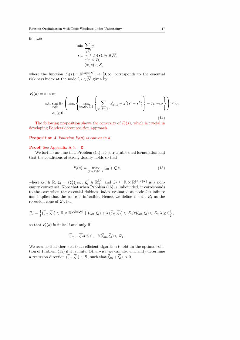
where the function Fl(s) : R|A|×|N| 7→ [0,∞] corresponds to the essentialriskiness index at the node l, l ∈ N given by
Fl(s) = min αl
s.t. supP∈F
EP
max
max
k∈N∪1
∑
a∈δ−(k)
slaτk + z′(sl − sk)
− τ l,−αl
≤ 0,
αl ≥ 0.(14)
The following proposition shows the convexity of Fl(s), which is crucial indeveloping Benders decomposition approach.
Proposition 4 Function Fl(s) is convex in s.
Proof. See Appendix A.5.
We further assume that Problem (14) has a tractable dual formulation andthat the conditions of strong duality holds so that
Fl(s) = max(ζl0,ζl
)∈Zl
ζl0 + ζ ′ls, (15)
where ζl0 ∈ R, ζl = (ζjl )j∈N , ζj
l ∈ R|A|+ and Zl ⊆ R × R|A|×|N| is a non-
empty convex set. Note that when Problem (15) is unbounded, it correspondsto the case when the essential riskiness index evaluated at node l is infiniteand implies that the route is infeasible. Hence, we define the set Rl as therecession cone of Zl, i.e.,
Rl =(ζl0, ζl
)∈ R× R|A|×|N| | (ζl0, ζl) + λ
(ζ l0, ζl
)∈ Zl, ∀(ζl0, ζl) ∈ Zl, λ ≥ 0
,
so that Fl(s) is finite if and only if
ζ l0 + ζ′ls ≤ 0, ∀(ζ l0, ζl) ∈ Rl.
We assume that there exists an efficient algorithm to obtain the optimal solu-tion of Problem (15) if it is finite. Otherwise, we can also efficiently determine
a recession direction (ζ l0, ζl) ∈ Rl such that ζl0 + ζ′
ls > 0.

18 Yu Zhang et al.
To solve Problem (7) using the Benders decomposition approach, we definethe restricted master problem at the t-th iteration as
min∑
l∈N
ηl
s.t. ζl0 + ζ ′ls ≤ ηl, ∀(ζl0, ζl) ∈ Zt
l , ∀l ∈ N ,
ζl0 + ζ′
ls ≤ 0, ∀(ζl0, ζl) ∈ Rtl , ∀l ∈ N ,
c′x ≤ B,
(x, s) ∈ S,
(16)
where Ztl and Rt
l are finite subsets of Zl and Rl respectively, for all l ∈ N .
Algorithm 1 (Benders decomposition)
Initialization: Set t := 1, Z1l := ∅ and R1
l := ∅, ∀l ∈ N .
1. Solve Problem (16) and let (x∗, s∗,η∗) be an optimal solution.2. For all l ∈ N , solve Problem (15). If Fl(s
∗) is finite, let the optimal solutionbe (ζl0, ζl) ∈ Zl. Otherwise, let (ζ l0, ζl) ∈ Rl be a recession direction such
that ζ l0 + ζl
′s∗ > 0.
3. If Fl(s∗) = η∗l for all l ∈ N then terminate algorithm and return optimal
route x∗.4. Set
Rt+1l := Rt
l ∪ (ζ l0, ζl) ∀l ∈ N : Fl(s∗) = ∞
and
Zt+1l := Zt
l ∪ (ζl0, ζl) ∀l ∈ N : Fl(s∗) ∈ (η∗l ,∞).
5. Set t := t+ 1. Go to Step 1.
Since the domain of variables (x, s) is finite, the algorithm must terminatebecause only finitely many subproblems can be defined.
Algorithm 1 presents a cutting-plane implementation, in which Bendersdual subproblems (15) would be solved only after the restricted master prob-lem (16) is solved to optimality. However, it is well-known that Benders de-composition can benefit in computational speed from using branch-and-cutimplementations (Vanderbeck and Wolsey 2010), in which Benders dual sub-problems (15) are solved at the restricted master problem (16)’s integer nodesand possibly at the fractional nodes of low depth, but not just at its optimalnode. The branch-and-cut variant of Algorithm 1 can be easily implemented inmodern integer programming solvers. In our computational study in Section7, we will use the IBM CPLEX general purpose integer programming solverto solve the restricted master problem in a branch-and-cut fashion, where theBenders cuts are added using the function ILOLAZYCONSTRAINTCALLBACK.
We next elaborate on how we can form and solve the dual problem (15)for several concrete cases of the primal problem (14). For sample average

Routing Optimization with Time Windows under Uncertainty 19
approximation, we write Problem (14) as
Fl(s) = min αl
s.t.∑
ω∈Ω
yω ≤ 0,
yω ≥ ξωlk(s), ∀k ∈ N ∪ 1, ω ∈ Ω,
yω ≥ −αl, ∀ω ∈ Ω,
αl ≥ 0,
(17)
where ξωlk(s) =∑
a∈δ−(k) slaτk + z(ω)′(sl − sk)− τ l.
Theorem 3 Let ξωl (s) = maxk∈N∪1 ξωlk(s) and let the index function ν :
Ω 7→ Ω be a permutation of Ω such that
ξν(1)l (s) ≥ ξ
ν(2)l (s) ≥ · · · ≥ ξ
ν(|Ω|)l (s).
If∑
ω∈Ω ξωl (s) > 0, then Fl(s) = ∞. Otherwise,
Fl(s) = max
maxi∈1,2,··· ,|Ω|−1
i∑
ω=1
ξν(ω)l (s)
|Ω| − i
, 0
. (18)
Proof. See Appendix A.6.Theorem 3 indicates that we can solve the Benders subproblems via a
sorting algorithm, which is a strongly polynomial time algorithm that scaleswell computationally with the number of samples, i.e., O(|Ω| log(|Ω|)). Whenimplementing the Benders decomposition for a given solution of the restrictedmaster problem, s∗, we determine for each l ∈ N , whether
∑
ω∈Ω ξωl (s
∗) > 0. Ifso, we extract the index function, κ∗(ω) ∈ argmaxk∈N∪1 ξ
ωlk(s
∗), determine
the affine relation such that∑
ω∈Ω ξωlκ∗(ω)(s
∗) = ζl0 + ζ′
ls∗, and add (ζ l0, ζl)
to the set Rtl . Specifically, ζl0 = −|Ω|τ l and, for a ∈ A and j ∈ N , ζ
j
la =∑
ω∈Ω ζjlaω , where
ζjlaω =
za(ω), if j = l 6= κ∗(ω), a ∈ A\δ−(κ∗(ω)),za(ω) + τκ∗(ω), if j = l 6= κ∗(ω), a ∈ δ−(κ∗(ω)),
−za(ω), if j = κ∗(ω) 6= l, a ∈ A,τκ∗(ω), if j = l = κ∗(ω), a ∈ δ−(κ∗(ω)),
0, otherwise.
If ξωl (s∗) ≤ 0 for all ω ∈ Ω, we obtain from (18) that Fl(s
∗) = 0. Otherwise,we have
Fl(s∗) =
i∗∑
ω=1
ξν(ω)lκ∗(ν(ω))(s
∗)
|Ω| − i∗
for some i∗ ∈ 1, . . . , |Ω|−1. Similarly, we can extract the affine relation suchthat Fl(s
∗) = ζl0 + ζ′ls
∗ and introduce (ζl0, ζl) to the set Ztl , where
ζl0 = − i∗
|Ω| − i∗τ l,
20 Yu Zhang et al.
and, for a ∈ A and j ∈ N ,
ζjla =
i∗∑
ν(ω)=1
ζjlaν(ω)
|Ω| − i∗.
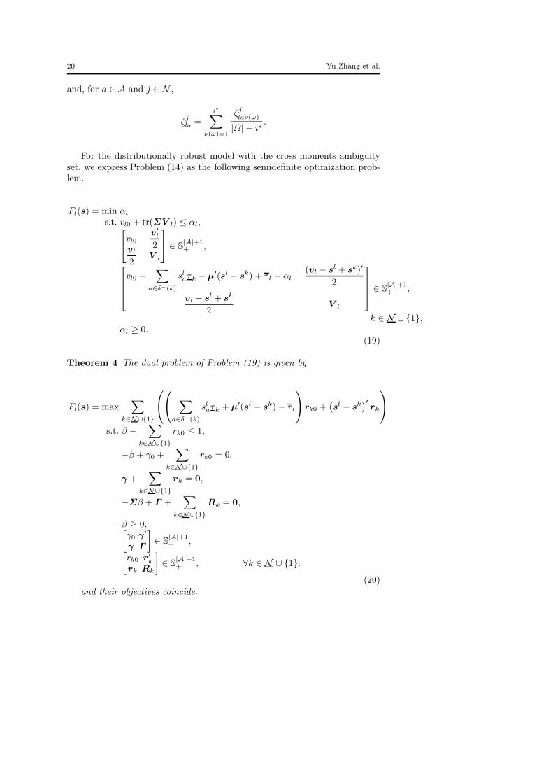
For the distributionally robust model with the cross moments ambiguityset, we express Problem (14) as the following semidefinite optimization prob-lem.
Fl(s) = min αl
s.t. vl0 + tr(ΣV l) ≤ αl,
vl0
v′l
2vl
2V l
∈ S|A|+1+ ,
vl0 −∑
a∈δ−(k)
slaτk − µ′(sl − sk) + τ l − αl(vl − sl + sk)′
2
vl − sl + sk
2V l
∈ S
|A|+1+ ,
k ∈ N ∪ 1,αl ≥ 0.
(19)
Theorem 4 The dual problem of Problem (19) is given by
Fl(s) = max∑
k∈N∪1
∑
a∈δ−(k)
slaτk + µ′(sl − sk)− τ l
rk0 +(sl − sk
)′rk
s.t. β −∑
k∈N∪1
rk0 ≤ 1,
−β + γ0 +∑
k∈N∪1
rk0 = 0,
γ +∑
k∈N∪1
rk = 0,
−Σβ + Γ +∑
k∈N∪1
Rk = 0,
β ≥ 0,[γ0 γ′
γ Γ
]
∈ S|A|+1+ ,
[rk0 r′
k
rk Rk
]
∈ S|A|+1+ , ∀k ∈ N ∪ 1.
(20)
and their objectives coincide.
Routing Optimization with Time Windows under Uncertainty 21
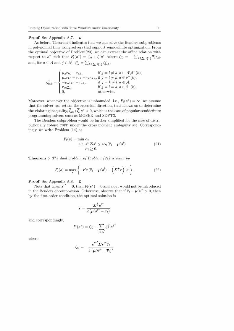
Proof. See Appendix A.7.
As before, Theorem 4 indicates that we can solve the Benders subproblemsin polynomial time using solvers that support semidefinite optimization. Fromthe optimal objective of Problem(20), we can extract the affine relation withrespect to s∗ such that Fl(s
∗) = ζl0 + ζ ′ls
∗, where ζl0 = −∑k∈N∪1 τ lrk0
and, for a ∈ A and j ∈ N , ζjla =∑
k∈N∪1 ζjlak,
ζjlak =
µark0 + rak, if j = l 6= k, a ∈ A\δ−(k),µark0 + rak + rk0τk, if j = l 6= k, a ∈ δ−(k),−µark0 − rak, if j = k 6= l, a ∈ A,rk0τk, if j = l = k, a ∈ δ−(k),0, otherwise.
Moreover, whenever the objective is unbounded, i.e., Fl(s∗) = ∞, we assume
that the solver can return the recession direction, that allows us to determine
the violating inequality, ζl0+ζ′ls
∗ > 0, which is the case of popular semidefiniteprogramming solvers such as MOSEK and SDPT3.
The Benders subproblem would be further simplified for the case of distri-butionally robust tspd under the cross moment ambiguity set. Correspond-ingly, we write Problem (14) as
Fl(s) = min αl
s.t. sl′Σsl ≤ 4αl(τ l − µ′sl)αl ≥ 0.
(21)
Theorem 5 The dual problem of Problem (21) is given by
Fl(s) = maxr
−r′r(τ l − µ′sl)−(
Σ12 r)′
sl
. (22)
Proof. See Appendix A.8.Note that when sl
∗= 0, then Fl(s
∗) = 0 and a cut would not be introducedin the Benders decomposition. Otherwise, observe that if τ l −µ′sl
∗> 0, then
by the first-order condition, the optimal solution is
r =Σ
12 sl
∗
2(µ′sl
∗ − τ l)
and correspondingly,
Fl(s∗) = ζl0 +
∑
j∈N
ζjl
′sj
∗
where
ζl0 = − sl∗′Σsl
∗τ l
4(µ′sl
∗ − τ l)2

22 Yu Zhang et al.
and
ζjl =
sl∗′Σsl
∗
4(µ′sl
∗ − τ l)2µ− 1
2(µ′sl
∗ − τ l)Σsl
∗, if j = l,
0, otherwise.
Note also that since Σ is positive definite, Problem (22) is unbounded whenτ l − µ′sl
∗ ≤ 0, in which case, observe that
r = −Σ12 sl
∗
is a recession direction. Correspondingly, we have
ζl0 = −sl∗′Σsl
∗τ l
and
ζj
l =
sl∗′Σsl
∗µ+Σsl
∗, if j = l,
0, otherwise.
6 Extensions
Apart from the essential riskiness index decision criterion, the results devel-oped in the paper can easily be extended to a travel cost minimization problemwith constraints that safeguard the risk of late arrivals defined via the popularConditional Value-at-Risk (CVaR) measure of Rockafellar and Uryasev (2000)defined as
CVaR1−ǫ (v) = minβ∈R
(
β +1
ǫEP
(
(v − β)+))
.
In particular, the constraint CVaR1−ǫ (v) ≤ 0 would imply that P(v ≤ 0) ≥1−ǫ. As it is well-known that CVaR is the best convex approximation of chanceconstrained problems (see, for instance, Nemirovski and Shapiro 2006), we canformulate the tsptw under uncertainty as
min c′x
s.t. CVaR1−ǫl (ξl(s, z)) ≤ 0, ∀l ∈ N ,
(x, s) ∈ S,(23)
which is a safe approximation for the chance constrained tsptw under uncer-tainty proposed in Laporte et al (1992) as follows,
min c′x
s.t. P (ξl(s, z) ≤ τ l) ≥ 1− ǫl, ∀l ∈ N ,
(x, s) ∈ S.(24)
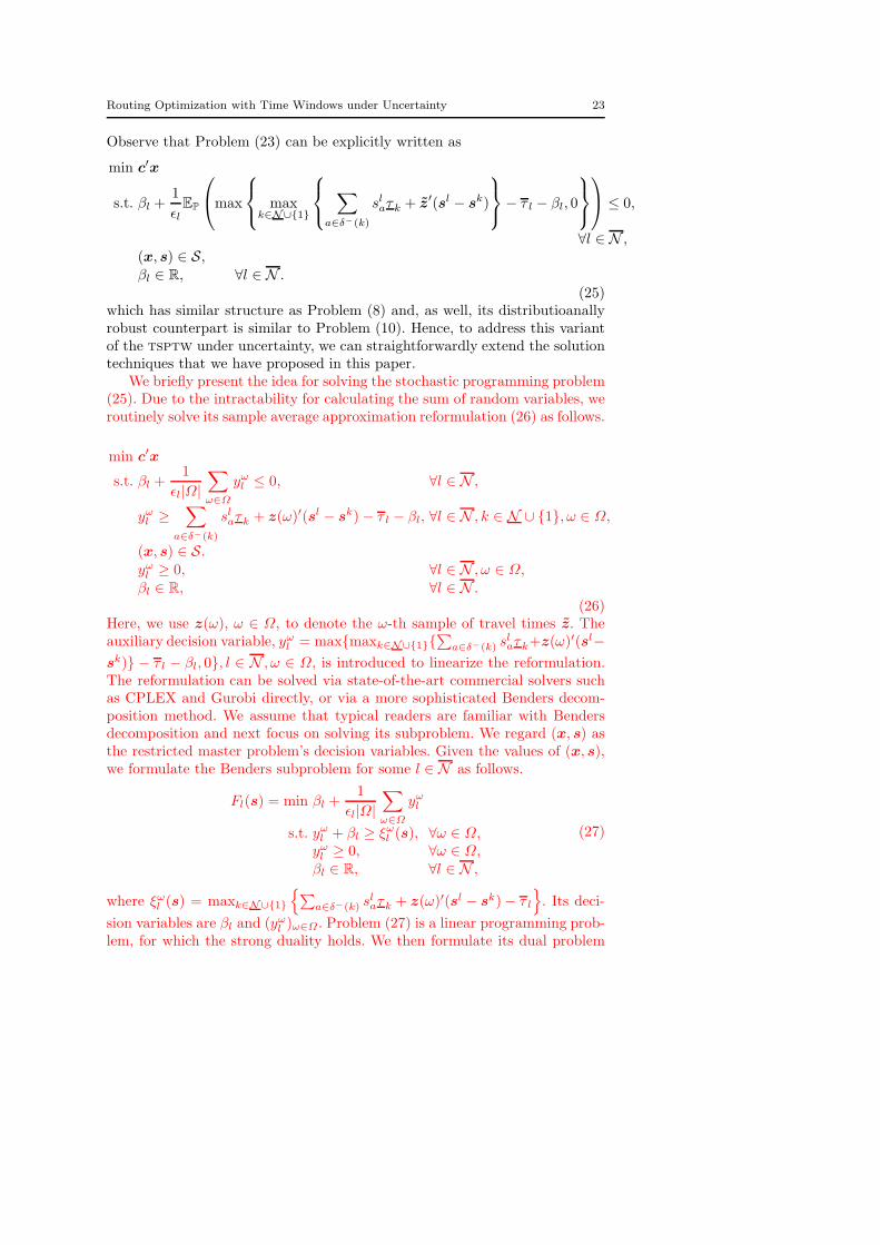
Routing Optimization with Time Windows under Uncertainty 23
Observe that Problem (23) can be explicitly written as
min c′x
s.t. βl +1
ǫlEP
max
max
k∈N∪1
∑
a∈δ−(k)
slaτk + z′(sl − sk)
− τ l − βl, 0
≤ 0,
∀l ∈ N ,
(x, s) ∈ S,βl ∈ R, ∀l ∈ N .
(25)which has similar structure as Problem (8) and, as well, its distributioanallyrobust counterpart is similar to Problem (10). Hence, to address this variantof the tsptw under uncertainty, we can straightforwardly extend the solutiontechniques that we have proposed in this paper.
We briefly present the idea for solving the stochastic programming problem(25). Due to the intractability for calculating the sum of random variables, weroutinely solve its sample average approximation reformulation (26) as follows.
min c′x
s.t. βl +1
ǫl|Ω|∑
ω∈Ω
yωl ≤ 0, ∀l ∈ N ,
yωl ≥∑
a∈δ−(k)
slaτk + z(ω)′(sl − sk)− τ l − βl, ∀l ∈ N , k ∈ N ∪ 1, ω ∈ Ω,
(x, s) ∈ S.yωl ≥ 0, ∀l ∈ N , ω ∈ Ω,
βl ∈ R, ∀l ∈ N .
(26)Here, we use z(ω), ω ∈ Ω, to denote the ω-th sample of travel times z. Theauxiliary decision variable, yωl = maxmaxk∈N∪1
∑
a∈δ−(k) slaτk+z(ω)′(sl−
sk) − τ l − βl, 0, l ∈ N , ω ∈ Ω, is introduced to linearize the reformulation.The reformulation can be solved via state-of-the-art commercial solvers suchas CPLEX and Gurobi directly, or via a more sophisticated Benders decom-position method. We assume that typical readers are familiar with Bendersdecomposition and next focus on solving its subproblem. We regard (x, s) asthe restricted master problem’s decision variables. Given the values of (x, s),we formulate the Benders subproblem for some l ∈ N as follows.
Fl(s) = min βl +1
ǫl|Ω|∑
ω∈Ω
yωl
s.t. yωl + βl ≥ ξωl (s), ∀ω ∈ Ω,
yωl ≥ 0, ∀ω ∈ Ω,
βl ∈ R, ∀l ∈ N ,
(27)
where ξωl (s) = maxk∈N∪1
∑
a∈δ−(k) slaτk + z(ω)′(sl − sk)− τ l
. Its deci-
sion variables are βl and (yωl )ω∈Ω. Problem (27) is a linear programming prob-lem, for which the strong duality holds. We then formulate its dual problem

24 Yu Zhang et al.
as follows.Fl(s) = max
∑
ω∈Ω
ξωl (s)pωl
s.t.∑
ω∈Ω
pωl = 1
pωl ≤ 1
ǫl|Ω| , ∀ω ∈ Ω,
pωl ≥ 0, ∀ω ∈ Ω,
(28)
in which (pωl )ω∈Ω are the decision variables. Observe that the objective func-tion can be interpreted as an expectation of a discrete random variable takingvalues at (ξωl (s))ω∈Ω with masses (pωl )ω∈Ω, respectively. To maximize the ex-pectation, we can sort (ξωl (s))ω∈Ω and greedily determine their masses. Specif-ically, we let the index function ν : Ω 7→ Ω be a permutation of Ω such that
ξν(1)l (s) ≥ ξ
ν(2)l (s) ≥ · · · ≥ ξ
ν(|Ω|)l (s).
We then assign mass 1ǫl|Ω| for each of the first ⌊ǫl|Ω|⌋ values, and the remaining
mass for the (⌊ǫl|Ω|⌋+ 1)-th value. Therefore, we have a closed-form solutionto the dual problem, given as follows.
Fl(s) =
⌊ǫl|Ω|⌋∑
i=1
ξν(i)l (s)
ǫl|Ω| +
1−⌊ǫl|Ω|⌋∑
i=1
1
ǫl|Ω|
ξν(⌊ǫl|Ω|⌋+1)l (s), (29)
where we define∑0
i=1 ξ = 0 and ξν(|Ω|+1)l = 0. The result can be rigorously
proved in a similar way as the proof of Theorem 3. We leave this and thedevelopment of the distributionally robust optimization method as an exerciseto the reader.
7 Computational Study
As a proof of concept of our proposed models, we perform numerical studies tounderstand their computational efficiency and to elucidate their effectivenessin mitigating travel and service times uncertainty in tsptw and tspd. In par-ticular, we consider a simple directed network of 12 nodes, N = 1, 2, · · · , 12with the nodes 1 and 12 being respectively the origin and the destination de-pots. The set of arcs is given by A = (i, j) | i ∈ N\n, j ∈ N\1, i 6=j, (i, j) 6= (1, 12) and hence, there are a total of |A| = 110 arcs. Let zTij and
zSi denote respectively the random travel time along arc (i, j) ∈ A and therandom service time at node i ∈ N . Note that the service times at nodes 1 and12 have zero values. By definition, we have zij = zSi + zTij for (i, j) ∈ A. We
assume that zTa , a ∈ A is a two-point independently distributed random vari-able with mean zTa so that P(zTa = (1−λa)zTa ) = P(zTa = (1+λa)z
Ta ) = 0.5 for
some λa > 0. Likewise, zSi , i ∈ N\1, 12 is also a similar two-point indepen-dently distributed random variable with mean zSi so that P(zSi = (1−λi)zSi ) =P(zSi = (1 + λi)z
Si ) = 0.5 for some λi > 0.

Routing Optimization with Time Windows under Uncertainty 25
The parameters zTa and zSi , a ∈ A, i ∈ N are given in Table 1 and for eachinstance of the problem, λa and λi are randomly and independently selectedfrom the set 0.1, 0.2, · · · , 0.8 with equal probability. These parameters of theproblem are adopted from the instance rbg010a of Ascheuer et al (2001). Forsimplicity, we do not impose a cost budget constraint in our experiments. Asshown in Table 1, three of the nodes have stipulated earliest arrival times andeight of the nodes have deadlines.
Table 1: The dataset for the tsptw
NzTa
zSi
τ τ1 2 3 4 5 6 7 8 9 10 11 12
1 - 0 0 0 0 0 0 0 0 0 0 - - - -2 - - 14 14 14 25 14 14 26 14 6 0 71 - 03 - 15 - 27 27 12 27 27 12 27 24 0 50 - 4004 - 10 24 - 24 16 24 24 18 24 23 0 64 - 4005 - 10 24 24 - 16 24 24 18 24 23 0 44 - 4006 - 24 0 0 0 - 0 0 29 0 14 0 51 300 6007 - 11 25 25 25 15 - 25 16 25 23 0 53 300 6008 - 16 18 18 18 24 18 - 24 18 12 0 51 300 6009 - 18 28 28 28 0 28 28 - 28 25 0 43 - -10 - 11 25 25 25 15 25 25 16 - 27 0 53 - -11 - 24 10 10 10 28 10 10 28 10 - 0 42 - -12 - - - - - - - - - - - - - - 700
7.1 Experiments with sample average approximation methods on tsptw
Suppose we have |Ω| independent samples of travel times z, (z(ω))ω∈Ω . Wesolve the stochastic tsptw through the following methods.
i) D: Solving the “deterministic” problem (3) that minimizes the travel costby a CPLEX solver, in which the travel times z are replaced with theirsample means |Ω|−1
∑
ω∈Ω z(ω). Hereafter, we let the travel costs c alsobe equal to |Ω|−1
∑
ω∈Ω z(ω) in values.ii) S-C: Solving Problem (26) that minimizes the travel cost subject to the
deadlines’ CVaR constraints by a CPLEX solver. Based on some prelim-inary results, we find that the solution performance is affected by theparameters ǫl ∈ (0, 1), l ∈ N . Small values for them may cause infeasibil-ity for the problem. In our experiments, we let ǫl = 0.8 for l ∈ N .
iii) S-C-B: Solving Problem (26) via the Benders decomposition algorithm de-scribed in Section 6, in which the Benders subproblems are solved throughFormula (29). We use a CPLEX solver to solve the restricted master prob-lem and invoke function ILOLAZYCONSTRAINTCALLBACK to add the Benderscuts in a branch-and-cut fashion. We let ǫl = 0.8 for l ∈ N .
iv) S-P: Solving Problem (4) that maximizes the joint on-time arrival proba-bility via solving the following sample average approximation reformula-

26 Yu Zhang et al.
tion (30) by a CPLEX solver.
max |Ω|−1∑
ω∈Ω Iω
s.t.∑
a∈δ−(k)
slaτk + z(ω)′(sl − sk
)− τ l ≤ (1− Iω)Ml, ∀k ∈ N ∪ 1, l ∈ N , ω ∈ Ω,
c′x ≤ B,
(x, s) ∈ S,Iω ∈ 0, 1, ∀ω ∈ Ω.
(30)Here, binary decision variable Iω indicates whether the vehicle arrivesat all nodes on time in sample ω ∈ Ω. If it does, Iω = 1, otherwiseIω = 0. Notation Ml, l ∈ N , represents a big number. We choose Ml :=maxk∈N τk+maxω∈Ω
∑
a∈A za(ω)−τ l, which is obviously an upper bound
of∑
a∈δ−(k) slaτk + z(ω)′
(sl − sk
)− τ l.
v) S-I: Solving Problem (9) that minimizes the sum of essential riskinessindexes by a CPLEX solver.
vi) S-I-B: Solving Problem (9) by the branch-and-cut implementation of theBenders decomposition algorithm described in Section 5, in which we solvethe Benders dual subproblems based on Theorem 3.
All these methods are implemented using the C++ language and the IBMCPLEX solver (ver 12.6). We adopt the 8-thread computation provided byCPLEX and impose a time limit of 3 hours, unless otherwise stated, for solv-ing each instance via each method. The experiments are run on a personalcomputer with a 4-core 3.2GHz CPU and a 8GB RAM.
For each of the above method under evaluation, we vary the the sample size,|Ω| ∈ 20, 50, 80, 100, 150 to understand its influence on the computationaltimes as well as the quality of the solutions. For a given sample size, we per-form 20 set of experiments. In each set, we randomly generate the parameters(λa)a∈A, (λi)i∈N\1,12 to first establish the probability distributions associ-ated with the random variables for the set of experiments. Subsequently, wesolve the problem using the method via sample average approximation wherewe generate |Ω| independent samples of z, (z(ω))ω∈Ω. In particular, we usethe same set of samples (z(ω))ω∈Ω to compute the optimal solutions for thevarious methods. Thereafter, to evaluate the performance of these solutions,we perform out-of-sample evaluation by generating another 20,000 indepen-dent samples of z. After completing the 20 set of experiments, we report theperformance by taking the average values of the individual indicators obtainedin each set. In particular, we focus on the following indicators:
i) ObjVal: the objective value,ii) Mean: the mean travel time,iii) LateProb: the lateness probability, i.e., P(∃i ∈ N|ξi(s, z) > 0),iv) ExpLate: the expected lateness, i.e.,
∑
i∈N E((ξi(s, z))+), and
v) ComTime: the wall-clock computational time (in seconds),vi) NoC/ToC: the number of the Benders cuts added/the total CPU time (in
seconds) used in solving the Benders subproblems,

Routing Optimization with Time Windows under Uncertainty 27
where ξ+ = maxξ, 0 and the probability P and the expectation E are eval-uated empirically using the 20, 000 out-of-sample data.
We report the solution performances for the various methods in Table2. The number in the bracket in column Method represents the number ofinstances without feasible solutions out of the 20 instances. When |Ω| = 3000,Methods S-C, S-P and S-I cannot solve each instance due to the time limitimposed. In contrast, we are able to obtain the optimal solution for MethodsS-I-B and S-I-C without much computational time.
Table 2: Performance comparison of different methods for solving the tsptw
Method |Ω| ObjVal Mean LatePro ExpLate ComTime NoC/ToCD
20
630.43 642.70 0.485 53.9 0.39 -S-C(3) 626.00 641.64 0.388 32.5 5.04 -
S-C-B(3) 626.00 641.64 0.388 32.5 1.83 118/1.48S-P 0.80 650.78 0.337 31.5 351.02 -S-I 23.69 646.22 0.309 23.3 394.48 -
S-I-B 23.69 646.22 0.309 23.3 460.31 119/3.66D
50
635.80 641.79 0.467 50.7 0.34 -S-C(1) 637.15 642.02 0.359 29.4 12.51 -
S-C-B(1) 637.15 642.02 0.359 29.4 2.26 153/3.39S-P 0.76 646.13 0.306 24.7 988.92 -S-I 28.44 644.35 0.294 19.8 1015.54 -
S-I-B 28.44 644.35 0.294 19.8 503.47 139/3.35D
80
637.44 641.48 0.490 56.4 0.46 -S-C 637.16 640.96 0.340 27.9 22.11 -
S-C-B 637.16 640.96 0.340 27.9 2.69 173/6.03S-P 0.74 646.16 0.308 25.8 2539.41 -S-I 27.68 644.78 0.293 19.2 2126.59 -
S-I-B 27.68 644.78 0.293 19.2 556.62 158/4.27D
100
635.41 641.63 0.486 59.1 0.35 -S-C 638.14 641.02 0.347 29.8 25.90 -
S-C-B 638.14 641.02 0.347 29.8 2.44 144/5.16S-P 0.75 646.86 0.301 25.1 3983.28 -S-I 26.11 645.02 0.292 19.4 3626.74 -
S-I-B 26.11 645.02 0.292 19.4 431.43 161/6.58D
150
638.17 641.42 0.485 55.2 0.39 -S-C 636.53 641.05 0.342 27.6 42.62 -
S-C-B 636.53 641.05 0.342 27.6 4.54 256/17.87S-P 0.74 646.33 0.293 23.4 7824.18 -S-I 27.52 644.42 0.288 19.3 6570.30 -
S-I-B 27.52 644.42 0.288 19.3 494.61 192/9.33D
3000
640.70 641.13 0.479 48.6 0.39 -S-C-B 639.81 640.96 0.351 23.4 68.27 328/401.98S-I-B 27.58 643.14 0.286 18.6 526.29 297/113.30
We conclude from Table 2 that Methods D, S-C, and S-C-I outperformMethods S-P, S-I, and S-I-B in terms of the average travel timeMean, while thelatter three methods are more effective in mitigating the lateness, as indicatedby LateProb and ExpLate. This phenomenon is a natural result of the objectivesof these methods.
28 Yu Zhang et al.
Method S-C presents a better performance than Method D in mitigatingthe lateness, and meanwhile is slightly better in reducing the average traveltime expect for the case of |Ω| = 50. Although Method D accounts for the meanvalues of travel times, its general poor performance may result from ignoringthe travel times’ dispersions. Method S-C provides a trade-off between the lowaverage travel time and the high likelihood of on-time arrivals.
We next focus on comparing the latter three methods regarding their per-formance in mitigating the lateness. We observe that the performance of bothindicators LateProb and ExpLate generally improves with the sample size, |Ω|,which is consistent with our expectations. In particular, Method S-I-B with3000 samples has the best performance. We also observe that for the samesample size, Method S-I outperforms Method S-P in both performance indi-cators, which could be rather surprising since we may have expected MethodS-P to have better performance on the LateProb indicator. Nevertheless, whenthe sample size is large enough, we would expect Method S-P to yield solu-tions that are at least as good over those of Method S-I on this indicator.However, on the flip side, it may also be computationally prohibitive to solvethese problems to optimality using Method S-P.
Method D consumes the least computational time and the time is insen-sitive to the sample size, which is consistent with our expectation since thedeterministic model has less decision variables and the number of decisionvariables is independent of the sample size. Method S-C requires more com-putational time; Methods S-P and S-I need far more. We also observe thatthe computational times of methods S-C, S-P and S-I are severely affected bythe sample size, |Ω| and are in stark contrast to Methods S-C-B and S-I-B,where the total computational times, the numbers of Benders cuts added, andthe computational times for solving Benders subproblems are only slightlyimpacted. Benders decomposition method S-C-B/S-I-B greatly improves thecomputational speed upon its counterpart S-C/S-I when |Ω| ≥ 50 in our exper-iment. As the sample size increases, the computational times of Methods S-Pand S-I increase super-linearly, with the former increasing at a faster rate thanthe latter. We note that the superior computational performance of MethodS-I-B underscores the effectiveness of the Benders decomposition approach.
In summary, we suggest the decision makers who attempt to minimizethe travel costs using Method S-C-B. Those who are seeking to mitigate thelateness are suggested choosing Method S-I-B. We encourage them to use alarge number of samples (e.g., |Ω| = 3000) in solving the problems.
7.2 Experiments with distributionally robust tspd
We had initially tried to extend the computational study to distributionallyrobust tsptw by implementing the corresponding branch-and-cut variant ofthe Benders decomposition algorithm described in Section 5, in which we useda MOSEK solver (ver 8.1) to obtain the solutions of the semidefinite program-ming subproblem based on Theorem 4. Preliminary results showed that it

Routing Optimization with Time Windows under Uncertainty 29
could take 4-8 minutes to obtain the optimal solution for each subproblem, orif unbounded, obtain its recession direction, and we were unable to obtain theoptimal solution for any of the instances of the distributionally robust tsptwwithin two days. The sluggish computational time might result from long timeto solve each Benders subproblem, a large number of Benders cuts to add, andthe inability to get MOSEK to solve subproblems in parallel. Hence, we aban-don the numerical study for tsptw and focus on distributionally robust tspd,where we can obtain the solutions to the subproblems easily.
We repeat the aforementioned computational study without the earliestarrival time τ in Table 1 so that the tsptw would be reduced to a tspd. Toconcentrate on comparing the methods for mitigating the lateness, we omitMethods D, S-C, and S-C-B, and indicator Mean. Apart from Methods S-P, S-I, and S-I-B, we introduce two more methods based on distributionally robustoptimization.
i) R-I-B: Solving the distributionally robust tspd (13) by the branch-and-cut implementation of the Benders decomposition algorithm described inSection 5, where the closed form solutions of the subproblems are com-puted via Theorem 5. In particular, the means µ and the covariance ma-trix Σ in the cross moment ambiguity set are estimated empirically fromthe samples of travel times, that is, we let µ = |Ω|−1
∑
ω∈Ω z(ω) and eachelement ofΣ, the covariance of za and za, a, a ∈ A, be |Ω|−1
∑
ω∈Ω(za(ω)−µa)(za(ω)− µa).
ii) R-RI-B: Solving the riskiness-index-based distributionally robust tspd
(31) by using a branch-and-cut implementation of the Benders decompo-sition algorithm proposed by Jaillet et al (2016).
inf∑
l∈N
αl
s.t. αl ln supP∈F
EP
(
exp
(z′sl − τ l
αl
))
≤ 0, ∀l ∈ N ,
c′x ≤ B,
(x, s) ∈ S,αl ≥ 0, ∀l ∈ N .
(31)
In this problem, the ambiguity set F is given as
F =
P ∈ P∣∣∣∣
EP(z) = µ,
P (z ∈ [z, z]) = 1,
,
where the means µ and supports [z, z] of travel times z are estimatedempirically from the samples. In particular, we let za = minω∈Ω za(ω)and za = maxω∈Ω za(ω) for a ∈ A. We regard (x, s) as the restrictedmaster problem’s decision variables and solve the Benders subproblem

30 Yu Zhang et al.
(32) for each l ∈ N using the technique proposed by Jaillet et al (2016).
inf αl
s.t. αl ln supP∈F
EP
(
exp
(z′sl − τ l
αl
))
≤ 0,
αl ≥ 0.
(32)
Table 3: Performance comparison of different methods for solving the tspd
Method |Ω| ObjVal LatePro ExpLate ComTime NoC/ToCS-P
20
0.81 0.337 28.3 89.26 -S-I 21.17 0.309 23.4 85.73 -
S-I-B 21.17 0.309 23.4 173.82 137/4.40R-RI-B 136.17 0.302 20.6 586.87 2524/91.87R-I-B 64.71 0.318 23.4 216.25 441/3.93
S-P
50
0.77 0.318 25.7 194.10 -S-I 26.65 0.291 19.6 176.39 -
S-I-B 26.65 0.291 19.6 195.70 178/5.42R-RI-B 123.95 0.290 18.8 627.40 2452/78.66R-I-B 73.08 0.301 19.9 213.95 438/4.05
S-P
80
0.75 0.302 23.6 340.23 -S-I 27.46 0.291 19.6 228.79 -
S-I-B 27.46 0.291 19.6 202.01 183/5.31R-RI-B 122.52 0.286 18.4 693.77 2845/103.58R-I-B 75.05 0.298 19.5 211.74 483/4.26
S-P
100
0.76 0.298 23.1 482.48 -S-I 24.22 0.289 19.3 335.92 -
S-I-B 24.22 0.289 19.3 208.76 185/6.18R-RI-B 119.11 0.287 18.3 689.77 2956/96.39R-I-B 69.67 0.296 19.5 201.22 456/3.92
S-P
150
0.74 0.286 20.3 902.31 -S-I 25.50 0.283 18.7 488.53 -
S-I-B 25.50 0.283 18.7 210.90 212/7.57R-RI-B 124.79 0.284 18.2 611.10 2675/80.44R-I-B 71.48 0.295 19.2 201.44 462/4.34
S-I-B
3000
26.40 0.279 18.2 216.23 332/81.27R-RI-B 123.14 0.285 18.2 637.37 2647/85.76R-I-B 73.26 0.287 18.6 189.98 479/3.69
We report the results in Table 3. When the number of samples is small,|Ω| ≤ 100, Method R-RI-B has the best performance in terms of LateProand ExpLate, but it requires significantly longer computational time than theothers. We expect Method R-RI-B to perform well because the travel timesare independently distributed, which can be exploited by the Aumann andSerrano (2008) riskiness index. Methods R-I-B and S-I-B performs reasonablywell against R-RI-B. Nonetheless, when we have 3000 samples of travel times,Method S-I-B has the best overall performance.
It is also interesting to note that despite the limited use of distributionalinformation, the performance of the distributionally robust tspd is relatively

Routing Optimization with Time Windows under Uncertainty 31
close to the stochastic tspd. Hence, since the actual distribution may not beavailable in many practical situations, it is reassuring that the solutions tothe distributioanlly robust tspd are near optimal. Moreover, to exemplify thebenefits of the distributional robust solutions, there are already computationalstudies suggesting that if the assumed distribution used in the sample averageapproximation deviates from the true distribution, the solutions may be infe-rior to those obtained from distributionally robust models (see, for instance,Adulyasak and Jaillet 2015).
8 Conclusions and future research
We study a tsptw with hard time windows under uncertain travel and ser-vice times. To quantify the risk associated with deadline violations, we proposethe essential riskiness index as the decision criterion to be minimized, whichhas the salient properties such as convexity for coherent decision making andcomputational needs. We also propose algorithms to minimize the index forthe tsptw via Benders decomposition technique based on sample average ap-proximation and distributionally robust formuations. We demonstrate througha computational study that that our approach can outperform the approachthat maximizes punctuality probability via sample average approximations.Apart from tsptw under uncertainty, the application of the essential riski-ness index is quite broad and can be applied in other contexts that may ariseinvolving multiple agents and the criterion will help them collectively attaintheir targets as well as possible under uncertainty. Nevertheless, we have yetto adequately address the computational efficiency of our approach as we areunable to solve larger sized problems within reasonable time. Hence, furtherwork will be needed to investigate how we can address larger sized problems,perhaps by leveraging on the state-of-the-art vehicle routing techniques in theliterature.
Acknowledgements
The authors would like to thank the anonymous reviewers and associate editorfor their extremely helpful suggestions and very thorough review of the paper.This paper is conducted when the first author works as a visiting student inNational University of Singapore, financially supported by the Chinese Schol-arship Council of the Ministry of Education, China. The last author is fundedby the National Natural Science Foundation of China (71420107028).
References
Adulyasak Y, Jaillet P (2015) Models and algorithms for stochastic and robust vehiclerouting with deadlines. Transportation Science

32 Yu Zhang et al.
Agra A, Christiansen M, Figueiredo R, Hvattum LM, Poss M, Requejo C (2012) Layeredformulation for the robust vehicle routing problem with time windows. In: LectureNotes in Computer Science, Springer Science Business Media, pp 249–260
Agra A, Christiansen M, Figueiredo R, Hvattum LM, Poss M, Requejo C (2013) The ro-bust vehicle routing problem with time windows. Computers & Operations Research40(3):856–866
Ascheuer N, Fischetti M, Grotschel M (2001) Solving the asymmetric travelling sales-man problem with time windows by branch-and-cut. Mathematical Programming90(3):475–506
Aumann RJ, Serrano R (2008) An economic index of riskiness. Journal of Political Economy116(5):810–836
Baldacci R, Bartolini E, Mingozzi A, Roberti R (2010) An exact solution frameworkfor a broad class of vehicle routing problems. Computational Management Science7(3):229–268
Baldacci R, Mingozzi A, Roberti R (2012) Recent exact algorithms for solving the vehiclerouting problem under capacity and time window constraints. European Journal ofOperational Research 218(1):1–6
Ben-Tal A, Nemirovski A (2001) Lectures on modern convex optimization: analysis, algo-rithms, and engineering applications, vol 2. Siam
Bertsimas D, Sim M (2003) Robust discrete optimization and network flows. MathematicalProgramming 98(1-3):49–71
Bertsimas D, Sim M, Zhang M (2017) A practically efficient approach for solving adaptivedistributionally robust linear optimization problems. Forthcoming in ManagementScience
Brown DB, Sim M (2009) Satisficing measures for analysis of risky positions. ManagementScience 55(1):71–84
Charnes A, Cooper WW (1959) Chance-constrained programming. Management science6(1):73–79
Claus A (1984) A new formulation for the travelling salesman problem. SIAM Journal onAlgebraic Discrete Methods 5(1):21–25
Dantzig GB, Ramser JH (1959) The truck dispatching problem. Management Science6(1):80–91
Dash S, Gunluk O, Lodi A, Tramontani A (2012) A time bucket formulation for the travelingsalesman problem with time windows. INFORMS Journal on Computing 24(1):132–147
Desaulniers G, Madsen OB, Ropke S (2014) Chapter 5: The vehicle routing problem withtime windows. In: Vehicle Routing: Problems, Methods, and Applications, SecondEdition, Society for Industrial & Applied Mathematics (SIAM), pp 119–159
Errico F, Desaulniers G, Gendreau M, Rei W, Rousseau LM (2016a) A priori optimizationwith recourse for the vehicle routing problem with hard time windows and stochasticservice times. European Journal of Operational Research 249(1):55–66
Errico F, Desaulniers G, Gendreau M, Rei W, Rousseau LM (2016b) The vehicle routingproblem with hard time windows and stochastic service times. EURO Journal onTransportation and Logistics pp 1–29
Fisher ML, Jornsten KO, Madsen OB (1997) Vehicle routing with time windows: Twooptimization algorithms. Operations Research 45(3):488–492
Gendreau M, Jabali O, Rei W (2014) Chapter 8: Stochastic vehicle routing problems. In:MOS-SIAM Series on Optimization, Society for Industrial and Applied Mathematics,pp 213–239
Gounaris CE, Wiesemann W, Floudas CA (2013) The robust capacitated vehicle routingproblem under demand uncertainty. Operations Research 61(3):677–693
Routing Optimization with Time Windows under Uncertainty 33
Gupta D, Denton B (2008) Appointment scheduling in health care: Challenges and oppor-tunities. IIE transactions 40(9):800–819
Isii K (1962) On sharpness of tchebycheff-type inequalities. Annals of the Institute of Sta-tistical Mathematics 14(1):185–197
Jaillet P, Qi J, Sim M (2016) Routing optimization under uncertainty. Operations Research64(1):186–200
Kao EPC (1978) A preference order dynamic program for a stochastic traveling salesmanproblem. Operations Research 26(6):1033–1045
Kenyon AS, Morton DP (2003) Stochastic vehicle routing with random travel times. Trans-portation Science 37(1):69–82
Laporte G (2009) Fifty years of vehicle routing. Transportation Science 43(4):408–416
Laporte G, Louveaux F, Mercure H (1992) The vehicle routing problem with stochastictravel times. Transportation Science 26(3):161–170
Lee C, Lee K, Park S (2011) Robust vehicle routing problem with deadlines and traveltime/demand uncertainty. J Oper Res Soc 63(9):1294–1306
Nemirovski A, Shapiro A (2006) Convex approximations of chance constrained programs.SIAM Journal on Optimization 17(4):969–996
Pecin D, Contardo C, Desaulniers G, Uchoa E (2017a) New enhancements for the exactsolution of the vehicle routing problem with time windows. INFORMS Journal onComputing 29(3):489–502
Pecin D, Pessoa A, Poggi M, Uchoa E (2017b) Improved branch-cut-and-price for capacitatedvehicle routing. Mathematical Programming Computation 9(1):61–100
Popescu I (2007) Robust mean-covariance solutions for stochastic optimization. OperationsResearch 55(1):98–112
Qi J (2016) Mitigating delays and unfairness in appointment systems. Management Science63(2):566–583
Rockafellar RT, Uryasev S (2000) Optimization of conditional value-at-risk. Journal of risk2:21–42
Scarf H, Arrow K, Karlin S (1958) A min-max solution of an inventory problem. Studies inthe mathematical theory of inventory and production 10:201–209
See CT, Sim M (2010) Robust approximation to multiperiod inventory management. Oper-ations research 58(3):583–594
Sniedovich M (1981) Technical note—analysis of a preference order traveling salesman prob-lem. Operations Research 29(6):1234–1237
Tas D, Gendreau M, Dellaert N, van Woensel T, de Kok A (2014) Vehicle routing with softtime windows and stochastic travel times: A column generation and branch-and-pricesolution approach. European Journal of Operational Research 236(3):789–799
Toth P, Vigo D (eds) (2014) Vehicle Routing: Problems, Methods, and Applications, SecondEdition. Society for Industrial & Applied Mathematics (SIAM), Philadelphia
Vanderbeck F, Wolsey LA (2010) Reformulation and decomposition of integer programs. 50Years of Integer Programming 1958-2008 pp 431–502
Verweij B, Ahmed S, Kleywegt AJ, Nemhauser G, Shapiro A (2003) The sample averageapproximation method applied to stochastic routing problems: a computational study.Computational Optimization and Applications 24(2-3):289–333
Wiesemann W, Kuhn D, Sim M (2014) Distributionally robust convex optimization. Oper-ations Research 62(6):1358–1376
Xin L, Goldberg DA, Shapiro A (2013) Time (in) consistency of multistage distributionallyrobust inventory models with moment constraints. arXiv preprint arXiv:13043074
Zhen J, den Hertog D, Sim M (2017) Adjustable robust optimization via fourier-motzkinelimination. Forthcoming in Operations Research

34 Yu Zhang et al.
A Proofs of Analytical Results
A.1 Proof of Proposition 2
It has been established that the variable sl, l ∈ N , represents the partial routefrom node 1 to node l along the route determined by x, say (1, i2), (i2, i3),· · · , (iκ−1, iκ
︸︷︷︸
=l
), · · · , (in−1, in︸︷︷︸
=n
) so that
sla =
1, if a ∈ (1, i2), (i2, i3), · · · , (iκ−1, l),0, otherwise
(33)
(see, for instance, Jaillet et al 2016). We have from Equation (1) that theservice commencement time at the node l can be determined recursively asfollows,
t1 = τ1 = 0,ti2 = maxt1 + z1i2 , τ i2,ti3 = maxti2 + zi2i3 , τ i3,
...tl = maxtiκ−1 + ziκ−1l, τ l.
Hence, we have
tl = max
max
· · ·maxmax
t1 + z1i2 , τ i2
+ zi2i3 , τ i3
· · · , τ iκ−1
+ ziκ−1l, τ l
= maxk∈1,i2,i3,··· ,iκ−1,l
τk +
∑
a∈(k,iκ+1),(iκ+1,iκ+2),··· ,(iκ−1,l)
za
,
(34)where k = iκ represents a node along the partial route from node 1 to node l.
Next we show that the service commencement time at node l can alsodetermined by Equation (2). For notational convenience, we define
tkl =∑
a∈δ−(k)
slaτk + z′(sl − sk
),
for all k ∈ N ∪ 1 and consider three cases as follows:
i) When k = 1, we have τ1 = 0 and s1 = 0 and hence, we have
t1l =∑
a∈δ−(1)
slaτ1 + z′(sl − s1) = τ1 +∑
a∈(1,i2),(i2,i3),··· ,(iκ−1,l)
za.
Moreover, t1l ≥ 0 because z ≥ 0.ii) When k ∈ i2, i3, · · · , iκ−1, l ∩ N , we have
∑
a∈δ−(k) sla = 1 and
tkl =∑
a∈δ−(k)
slaτk + z′(sl − sk) = τk +∑
a∈(k,iκ+1),(iκ+1,iκ+2),··· ,(iκ−1,l)
za.

Routing Optimization with Time Windows under Uncertainty 35
iii) When k ∈ iκ+1, iκ+2, · · · , n ∩ N , we have∑
a∈δ−(k) sla = 0 and (sl −
sk) ≤ 0. Since z ≥ 0, we have
tkl =∑
a∈δ−(k)
slaτk + z′(sl − sk) ≤ 0 ≤ t1l .
Hence, maxt1l , tkl = t1l for all k ∈ iκ+1, iκ+2, · · · , n ∩ N .
Observe that we can express Equation (2) as
tl = maxk∈N∪1
tkl = maxk∈1∪(i2,i3,··· ,iκ−1,l∩N )
τk +
∑
a∈(k,iκ+1),(iκ+1,iκ+2),··· ,(iκ−1,l)
za
.
(35)We note that for all k ∈ i2, i3, · · · , iκ−1, l\N we have τk = 0 and sincez ≥ 0, we also have
τk+∑
a∈(k,iκ+1),(iκ+1,iκ+2),··· ,(iκ−1,l)
za ≤ τ1+∑
a∈(1,i2),(i2,i3),··· ,(k,iκ+1),··· ,(iκ−1,l)
za = t1l .
Hence, maxt1l , tkl = t1l for all k ∈ i2, i3, · · · , iκ−1, l\N . Therefore, takingthese conditions into account, we have shown the equivalence of Equations(34), (35) and (2).
A.2 Proof of Proposition 3
i) Satisficing: If P(
ξ ≤ 0)
= 1, then EP
(
maxξ,−α)
≤ 0 for all α ≥ 0
and ρE(ξ) = 0. Conversely, if ρE(ξ) = 0, we have EP
(
maxξ, 0)
≤ 0,
which implies P(
ξ ≤ 0)
= 1.
ii) Infeasibility: For any α ∈ [0,∞), if EP
(
ξ)
> 0, then EP
(
maxξ,−α)
>
0. However, the definition requires
EP
(
maxξ,−α)
≤ 0.
We conclude that ρE(ξ) = min ∅ = ∞.
iii) Convexity:We denote α∗1 = ρE
(
ξ1
)
and α∗2 = ρE
(
ξ2
)
. Hence, EP
(
maxξ1,−α∗1)
≤0 and EP
(
maxξ2,−α∗2)
≤ 0. Since the function EP
(
maxξ,−α)
is
jointly convex in ξ and α, we have for λ ∈ [0, 1],
EP
(
maxλξ1 + (1 − λ)ξ2,− (λα∗1 + (1− λ)α∗
2))
≤ λEP
(
maxξ1,−α∗1)
+ (1− λ)EP
(
maxξ2,−α∗2)
≤ 0.
36 Yu Zhang et al.
Hence, αλ = λα∗1+(1−λ)α∗
2 satisfies EP
(
maxλξ1 + (1− λ)ξ2,−αλ)
≤0 and ρE
(
λξ1 + (1− λ)ξ2
)
≤ αλ = λρE
(
ξ1
)
+ (1− λ)ρE
(
ξ2
)
.
iv) Delay bounds: The bound is true for ρE
(
ξ)
= ∞ and ρE
(
ξ)
= 0, since
the latter would imply P
(
ξ > 0)
= 0. For ρE
(
ξ)
∈ (0,∞), we let α∗ =
ρE
(
ξ)
and hence we have
P
(
ξ > α∗θ)
= P
(
ξ + α∗ > α∗θ + α∗)
≤ P
((
ξ + α∗)+
> α∗(1 + θ)
)
≤E
(
(ξ + α∗)+)
α∗(1 + θ)
≤ α∗
α∗(1 + θ)
=1
1 + θ.
The second inequality holds because of Markov inequality; the third in-
equality is due to EP
(
maxξ + α∗, 0)
≤ α∗, implied by the definition.
A.3 Proof of Theorem 1
We denote u = z − µ and rewrite the ambiguity set as
G =
Q ∈ P∣∣∣∣
EQ(u) = 0EQ
(uu′
)= Σ
.
For each l ∈ N , we determine the worse-case expectation
supQ∈G
EQ
max
max
k∈N∪1
∑
a∈δ−(k)
slaτk + (u+ µ)′(sl − sk)
− τ l + αl, 0
by formulating the following optimization problem:
sup
∫
R|A|
max
max
k∈N∪1
∑
a∈δ−(k)
slaτk + (u+ µ)′(sl − sk
)
− τ l + αl, 0
dQ
s.t.
∫
R|A|
u dQ = 0,∫
R|A|
uu′ dQ = Σ,∫
R|A|
dQ = 1,
dQ ≥ 0.

Routing Optimization with Time Windows under Uncertainty 37
Its dual problem is given as
inf vl0 + tr(ΣV l)s.t. vl0 + u′vl + u′V lu ≥ 0, ∀u ∈ R|A|,
vl0 + u′vl + u′V lu ≥∑
a∈δ−(k)
slaτk + (u + µ)′(sl − sk)− τ l + αl, ∀k ∈ N ∪ 1,
u ∈ R|A|,
(36)for which strong duality holds and their objectives coincide (see, for instance,Isii 1962). We express the first constraint in Problem (36) equivalently as
[1u
]′
vl0
v′l
2vl
2V l
[1u
]
≥ 0, ∀u ∈ R|A|,
or further as
vl0
v′l
2vl
2V l
∈ S|A|+1+ .
Similarly, we express the second constraint in Problem (36) equivalently as
vl0 −∑
a∈δ−(k)
slaτk − µ′(sl − sk) + τ l − αl(vl − sl + sk)′
2
vl − sl + sk
2V l
∈ S
|A|+1+ .
Hence, the first constraint of Problem (10) is satisfied if and only if thereexists vl0 ∈ R, vl ∈ R|A| and V l ∈ R|A|×|A| for l ∈ N that are feasible in thefollowing system of conic constraints,
vl0 + tr(ΣV l) ≤ αl, ∀l ∈ N ,
vl0
v′l
2vl
2V l
∈ S|A|+1+ , ∀l ∈ N ,
vl0 −∑
a∈δ−(k)
slaτk − µ′(sl − sk) + τ l − αl(vl − sl + sk)′
2
vl − sl + sk
2V l
∈ S
|A|+1+ , ∀l ∈ N ,
k ∈ N ∪ 1.
Substituting them in Problem (10), we obtain Problem (11).

38 Yu Zhang et al.
A.4 Proof of Theorem 2
It suffices to show that for a given s0 ∈ R, s ∈ R|A|, s 6= 0, α ≥ 0, the followingconstraints are feasible
v0 + tr(ΣV ) ≤ α
v0 − s0(v − s)′
2v − s
2V
∈ S
|A|+1+ ,
v0
v′
2v
2V
∈ S|A|+1+ ,
(37)
for some v0 ∈ R,v ∈ R|A|,V ∈ S|A|+ if and only if
s′Σs ≤ 4α(α− s0). (38)
For the “if” direction, suppose the constraint (38) is feasible, since s′Σ′s > 0,we would have α > 0 and α− s0 > 0. Let
v0 =
(
s0 +√
s20 + s′Σs)2
4√
s20 + s′Σs,
v =
(
s0 +√
s20 + s′Σs)
s
2√
s20 + s′Σs,
V =ss′
4√
s20 + s′Σs.
Observe that for all u ∈ R|A|,
[1u
]′
v0
v′
2v
2V
[1u
]
=
(
s0 +√
s20 + s′Σs)2
4√
s20 + s′Σs+
(
s0 +√
s20 + s′Σs)
2√
s20 + s′Σss′u+
(s′u)2
4√
s20 + s′Σs
=
(
s0 +√
s20 + s′Σs+ s′u)2
4√
s20 + s′Σs≥ 0,

Routing Optimization with Time Windows under Uncertainty 39
and
[1u
]′
v0 − s0(v − s)′
2(v − s)
2V
[1u
]
=
(
s0 +√
s20 + s′Σs)2
4√
s20 + s′Σs− s0 +
(
s0 +√
s20 + s′Σs)
2√
s20 + s′Σs− 1
s′u+(s′u)2
4√
s20 + s′Σs
=
(
s0 −√
s20 + s′Σs)2
4√
s20 + s′Σs+
(
s0 −√
s20 + s′Σs)
2√
s20 + s′Σss′u+
(s′u)2
4√
s20 + s′Σs
=
(
s0 −√
s20 + s′Σs+ s′u)2
4√
s20 + s′Σs≥ 0.
Moreover,
s′Σs ≤ 4α(α− s0)⇒ s20 + s′Σs ≤ (2α− s0)
2
⇒√
s20 + s′Σs ≤ 2α− s0 since 2α− s0 > α− s0 > 0
⇒ 1
2s0 +
1
2
√
s0 + s′Σs ≤ α
⇒ 2s0√
s20 + s′Σs+ 2(s20 + s′Σs)
4√
s20 + s′Σs≤ α since s′Σs > 0
⇒
(
s0 +√
s20 + s′Σs)2
4√
s20 + s′Σs+
s′Σs
4√
s20 + s′Σs≤ α
⇒ v0 + tr(ΣV ) ≤ α.
Hence, the constraints in (37) are also feasible.Conversely, suppose the constraints in (37) are feasible for some v0 ∈ R,v ∈
R|A|,V ∈ S|A|+ . Let
r0 =1
2+
s0
2√
s20 + s′Σs,
r =Σs
2√
s20 + s′Σs,
Note that since sΣs > 0, we have r0 ∈ (0, 1). Observe that
[r0 r′
r 1r0rr′
]
∈ S|A|+ and
[1− r0 −r′
−r Σ − 1r0rr′
]
∈ S|A|+
since for all w ∈ R|A|,
[1w
]′ [r0 r′
r 1r0rr′
] [1w
]
= r0 + 2r′w +1
r0(r′w)2 =
(√r0 +
1√r0
r′w
)2
≥ 0

40 Yu Zhang et al.
and[1w
]′ [1− r0 −r′
−r Σ − 1r0rr′
] [1w
]
= 1− r0 − 2r′w − 1
r0(r′w)2 +w′Σw
=
(√1− r0 −
1√1− r0
r′w
)2
−(
1
r0+
1
1− r0
)
(r′w)2 +w′Σw
≥ − 1
r0(1− r0)(r′w)2 +w′Σw
= −4(s20 + s′Σs
)
s′Σs(r′w)2 +w′Σw
= − 1
s′Σs(w′Σs)2 +w′Σw
= − 1
s′Σs((Σ1/2w)′Σ1/2s)2 +w′Σw
≥ − 1
s′Σs(s′Σs)(w′Σw) +w′Σw Cauchy-Schwarz inequality
= 0.
Therefore,
tr
v0
v′
2v
2V
[1− r0 −r′
−r Σ − 1r0rr′
]
+tr
v0 − s0(v − s)′
2v − s
2V
[r0 r′
r 1r0rr′
]
≥ 0
or equivalently
v0 + tr(ΣV ) ≥ s0r0 + r′s =1
2s0 +
1
2
√
s20 + s′Σs.
Hence,1
2s0 +
1
2
√
s20 + s′Σs ≤ v0 + tr(ΣV ) ≤ α,
which implies the feasibility of the constraint (38).
A.5 Proof of Proposition 4
Denote the optimal solutions of Problem (14) with s being s and s by αl andαl, respectively, so that Fl(s) = αl and Fl(s) = αl. To prove the convexity ofFl(s) by definition, we shall prove Fl(λs+ (1 − λ)s) ≤ λFl(s) + (1 − λ)Fl(s)for any λ ∈ [0, 1].
Observe that the left-hand side function of the first constraint in Problem(14), g(s, αl) = supP∈FEP
(
max
maxk∈N∪1
∑
a∈δ−(k) slaτk + z′(sl − sk)
− τ l,−αl
)
,
is convex piecewise affine in (s, αl). We then have, for any λ ∈ [0, 1],
g (λs+ (1− λ)s, λα+ (1 − λ)α) ≤ λg(s, α) + (1− λ)g(s, α),≤ λ0 + (1− λ)0.= 0.

Routing Optimization with Time Windows under Uncertainty 41
Also note that λα+ (1− λ)α ≥ 0. Hence, λα+ (1− λ)α is a feasible solutionto Problem (14) with s being λs+ (1− λ)s. As a result,
Fl(λs+ (1 − λ)s) ≤ λα + (1− λ)α = λFl(s) + (1 − λ)Fl(s).
This completes the proof.
A.6 Proof of Theorem 3
We specify the dual problem of Problem (17) as follows,
Fl(s) = max∑
ω∈Ω
∑
k∈N∪1
ξωlk(s)rωk
s.t. −ψ +∑
k∈N∪1
rωk + qω = 0, ∀ω ∈ Ω,
∑
ω∈Ω
qω ≤ 1,
ψ ≥ 0,rωk ≥ 0, k ∈ N ∪ 1, ω ∈ Ω,
qω ≥ 0, ∀ω ∈ Ω,
(39)
which we claim is equivalent to the following problem,
Fl(s) = max∑
ω∈Ω
ξωl (s)pω
s.t. |Ω|pω −∑
i∈Ω
pi ≤ 1, ∀ω ∈ Ω,
pω ≥ 0, ∀ω ∈ Ω.
(40)
We next prove the claim. For an optimal solution (ψ, r, q) to Problem (39),we infer from the first and the fifth constraints that ψ ≥ ∑
k∈N∪1 rωk ,
∀ω ∈ Ω, and therefore, qi = ψ−∑k∈N∪1 rik ≥∑k∈N∪1 r
ωk −
∑
k∈N∪1 rik,
∀i, ω ∈ Ω. This inequality and the second constraint in Problem (39) implythat |Ω|∑k∈N∪1 r
ωk −∑k∈N∪1
∑
i∈Ω rik ≤ 1, ∀ω ∈ Ω. Hence, the solu-
tion pω :=∑
k∈N∪1 rωk , ∀ω ∈ Ω, is clearly feasible in Problem (40). Since,
by definition ξωl (s) = maxk∈N∪1 ξωlk(s), it follows that Fl(s) ≥ Fl(s). Con-
versely, for an optimal solution p to Problem (40), we construct a solutionto Problem (39) as follows. Let rωκ∗(ω) := pω for all ω ∈ Ω where κ∗(ω) ∈argmaxk∈N∪1 ξ
ωlk(s), r
ωk := 0 for all ω ∈ Ω and k ∈ N ∪ 1\κ∗(ω),
ψ := maxω∈Ω pω, and qω := maxi∈Ω p
i − pω for all ω ∈ Ω. We can verifythat the solution is feasible and the objective value is equal to Fl(s). In par-ticular, Constraint
∑
ω∈Ω qω ≤ 1 is feasible since |Ω|pω −∑i∈Ω p
i ≤ 1 for all
ω ∈ argmaxi∈Ω pi. Hence, Fl(s) ≥ Fl(s). We then conclude that Fl(s) = Fl(s)
and the two problems are equivalent. Observe that 0 is a feasible solutionto Problem (40); the problem then can be bounded optimal or unbounded.
42 Yu Zhang et al.
Since strong duality holds for linear programming problems, we also haveFl(s) = Fl(s).
We next solve Problem (40). The problem is unbounded if and only if thereexists a recession direction p 6= 0, |Ω|pω −∑i∈Ω p
i ≤ 0 and pω ≥ 0 for ω ∈ Ω,such that
∑
ω∈Ω ξωl (s)p
ω > 0. The recession direction should satisfy p1 =
p2 = · · · = p|Ω| > 0, or otherwise the constraint |Ω|pω−∑i∈Ω pi ≤ 0 would be
violated for all ω ∈ argmaxi∈Ω pi. Hence, the condition
∑
ω∈Ω ξωl (s)p
ω > 0 isequivalent to
∑
ω∈Ω ξωl (s) > 0, and in which case, the problem is unbounded
and Fl(s) = ∞.If the problem is bounded and optimal, there exists an optimal extreme
point solution, which is determined by selecting |Ω| binding constraints inProblem (40). Observe that for a given ω ∈ Ω the constraints pω ≥ 0 and|Ω|pω −∑i∈Ω p
i ≤ 1 cannot be simultaneously binding because it would im-ply that −∑i∈Ω\ω p
i = 1, which contradicts with the nonnegativity of p.
Hence, partition Ω into two subsets Ω1 and Ω2, such that |Ω|pω−∑i∈Ω pi = 1,
∀ω ∈ Ω1 and pω = 0, ∀ω ∈ Ω2. When Ω1 = ∅, we have p = 0 being an extremepoint with objective value of zero. We also note that |Ω1| = |Ω| is inadmissiblebecause we would have
∑
ω∈Ω(|Ω|pω−∑i∈Ω pi) =
∑
ω∈Ω 1, which is a contra-diction unless |Ω| = 0. When 1 ≤ |Ω1| ≤ |Ω|−1, we solve for the system of lin-ear equations, |Ω|pω −∑i∈Ω p
i = 1, ∀ω ∈ Ω1, or equivalently, (|Ω|I−ee′)p =
e, where I is the unit diagonal matrix in R|Ω1|×|Ω1|, p = (pω)′ω∈Ω1, and e is
the vector of ones in R|Ω1|. Observe that p = 1|Ω|−|Ω1|
e is a feasible solution.
Moreover, it is the unique solution because (|Ω|I − ee′) is invertible and wecan verify that (|Ω|I−ee′)( 1
|Ω|I+1
|Ω|(|Ω|−|Ω1|)ee′) = I. Hence, pω = 1
|Ω|−|Ω1|,
∀ω ∈ Ω1 and pω = 0, ∀ω ∈ Ω2 is an extreme point solution. Observe that atoptimality, Ω1 would correspond to the set ν(1), ν(2), · · · , ν(|Ω1|) and the
objective value would be∑|Ω1|
ω=1ξν(ω)l
(s)|Ω|−|Ω1|
. Finally, we conclude that
Fl(s) = max
maxi∈1,2,··· ,|Ω|−1
i∑
ω=1
ξν(ω)l (s)
|Ω| − i
, 0
,
and the result follows.
A.7 Proof of Theorem 4
Let β,
[γ0, γ
′
γ, Γ
]
, and
[rk0, r
′k
rk, Rk
]
, k ∈ N∪1, be the dual variables correspond-
ing to the first three constraints in Problem (19), respectively, where γ ∈ R|A|,Γ ∈ R|A|×|A|, rk ∈ R|A|, Rk ∈ R|A|×|A|. Based on the theory of conic duality(see, for instance, Ben-Tal and Nemirovski 2001), we obtain its dual problem(20). Moreover, their objectives coincide because the Slater’s condition holds,i.e., there exists a strictly relative interior point for Problem (20), defined as
β = 1, γ0 = rk0 = 1|N |+2 , γ = rk = 0, and Γ = Rk = Σ
|N |+2 , k ∈ N ∪ 1,

Routing Optimization with Time Windows under Uncertainty 43
such thatβ −
∑
k∈N∪1
rk0 < 1,
−β + γ0 +∑
k∈N∪1
rk0 = 0,
γ +∑
k∈N∪1
rk = 0,
−Σβ + Γ +∑
k∈N∪1
Rk = 0,
β > 0,[γ0 γ′
γ Γ
]
∈ S|A|+1++ ,
[rk0 r′
k
rk Rk
]
∈ S|A|+1++ , ∀k ∈ N ∪ 1,
where S|A|+1++ represents the set of symmetric positive definite matrices in
R(|A|+1)×(|A|+1). The last two constraints hold because
Σ ∈ S|A|++ ⇔
1
|N |+ 20′
0Σ
|N |+ 2
∈ S
|A|+1++ .
A.8 Proof of Theorem 5
Given a restricted master problem’s solution s∗, we denote the objective valuesof Problem (21) and (22) by F (s∗) and F (s∗), respectively. When sl
∗= 0, we
observe that F (s∗) = F (s∗) = 0. Otherwise, if τ l −µ′sl∗> 0, it is easy to see
that
F (s∗) =sl
∗′Σsl
∗
4(τ l − µ′sl∗).
Based on the first-order condition, the optimal solution of Problem (22) is
r =Σ
12 sl
∗
2(µ′sl
∗ − τ l)
and correspondingly,
F (s∗) =sl
∗′Σsl
∗
4(τ l − µ′sl∗)= F (s∗).
If τ l −µ′sl∗ ≤ 0, since Σ is positive definite, we observe that Problem (21) is
infeasible and F (s∗) = ∞. Observe also that
r = −Σ12 sl
∗
is an recession direction to Problem (22) such that F (s∗) = ∞ = F (s∗).Hence, the result follows.