1

LINEARIZED ORBIT COVARIANCE GENERATION AND

PROPAGATION ANALYSIS VIA SIMPLE MONTE CARLO SIMULATIONS

Chris Sabol*, Thomas Sukut†, Keric Hill‡, Kyle T. Alfriend§,

Brendan Wright**, You Li**, and Paul Schumacher*

Monte Carlo simulations are used to explore how well covariance represents orbit state estimation and prediction errors when fitting to normally distributed, zero mean error observation data. The covariance is generated as a product of a least-squares differential corrector, which estimates the state in either Cartesian coordinates or mean equinoctial elements, and propagated using linearized dynamics. Radar range and angles observations of a LEO satellite are generated for either a single two-minute radar pass or catalog-class scenario. State error distributions at the estimation epoch and after propagation are analyzed in Cartesian, equinoctial, or curvilinear coordinates. Results show that the covariance is representative of the state error distribution at the estimation epoch for all state representations; however, the Cartesian representation of the covariance rapidly fails to represent the error distribution when propagated away from epoch due to the linear nature of the comparison coordinate system, not the linearization of the dynamics used in the covariance propagation. Analysis demonstrates that dynamic nonlinearity ultimately drives the error distribution to be non-Gaussian in element space despite the fact that sample distribution second moment terms appear to remain consistent with the propagated covariance. Lastly, the results show the importance of using as much precision as possible when dealing with ill-conditioned covariance matrices.

INTRODUCTION As part of the orbit estimation process, state uncertainties are often derived from covariance information. For weighted batch least squares and Kalman-type filtering approaches, the covariance information gives the trajectory error ellipsoid provided certain assumptions are met.1 These assumptions usually include independent, normally distributed, zero mean observation errors and representative linearized dynamics. This paper uses simple Monte Carlo simulations to explore how well the covariance represents orbit state estimation errors when the independent, normally distributed, zero mean observation error assumption is met. The covariance is estimated and propagated using the linear state transition matrix in both Cartesian and mean equinoctial states, and state error distributions are considered in Cartesian, equinoctial, and curvilinear coordinates. Meaningful orbit error distribution functions are the cornerstone to dynamic command and control applications, and many current approaches assume a Gaussian distribution, which is represented by a linearly propagated covariance matrix. Sensor tasking, track association, and * Research Aerospace Engineer, Air Force Maui Optical and Supercomputing, Directed Energy Directorate, Air Force Research Laboratory, 535 Lipoa Parkway, Suite 200, Kihei, HI 96753 † Cadet 1st Class, Astronautics Department, United States Air Force Academy, Colorado Springs, CO 80840 ‡ Senior Scientist, Pacific Defense Solutions, 1300 N. Holopono St., Suite 116, Kihei, HI 96753 § TEES Distinguished Research Chair Professor, Texas A&M University, Dept of Aerospace Engineering, 3141 TAMU, College Station, TX 77843-3141 ** Cadet Captain, United States Military Academy, West Point, NY 10996

2

probability of collision calculations are all example applications that aim to take advantage of covariance information.2-5 This paper does not address the large spectrum of reasons why covariance information may not be representative of the true orbit error distribution function, such as non-Gaussian and autocorrelated observation errors and unmodeled perturbations. The analysis documented here ensures zero mean Gaussian observation errors and well modeled dynamics to focus on the common practice of using linearized state transition dynamics to form and propagate covariance information as a representation of the orbit error distribution. The analysis framework has been established to allow investigation of the impact of non-Gaussian and autocorrelated observation errors as well as mismodeled dynamics, which may be the subject of future work. This is not a new subject of research. Junkins, et al, developed a linearity index and compared the performance of linear covariance propagation in Cartesian, polar, and Keplerian element-based orbit states.6 These results demonstrated that an element-based formulation maintains a Gaussian distribution better than the polar and much better than the Cartesian representations. The analysis did not, however, form the initial covariance from observation data or make an attempt to separate impact of the linearized dynamics and the comparison frame. This work demonstrates that one should make a distinction between the two. Park and Scheeres investigated the use of incorporating higher order effects into the uncertainty propagation and also developed a nonlinearity index to indicate when these effects were important.7 While the mathematical development is applicable to all state representations, their analysis focused on Cartesian states and it is again unclear whether the higher order terms are accounting for dynamic nonlinearities or attempting to describe a bending distribution in linear coordinate space. Vallado and Seago studied covariance realism using real data test cases.8 This analysis provided great insight into various metrics used to describe how Gaussian the error distribution is and, being based on real data, the results do reflect real world conditions; however, the analysis was limited to Cartesian space, a great deal of the analysis focused on comparing position error standard deviations to the covariance based predictions, which is admittedly insufficient, and one cannot distinguish what is the root cause of any differences that arise. Similarly Kelecy and Jah have used Monte Carlo analysis to evaluate orbit error distributions in the presence of nonconservative dynamic mismodeling, but do not distinguish whether the observed non-Gaussian error distributions are due to the dynamic mismodeling or the limitations of the Cartesian state representation as demonstrated by Junkins, et al, and reproduced here.9 Lastly, Denham and Pines considered the impact of linearizing the observation-state mapping (measurement partials) in the formation of the Kalman gain; based on the findings of that work, the cases considered here should be insensitive to those effects but it is mentioned since many current orbit determination scenarios may be sensitive to this assumption.10

The rest of this paper describes how the simple Monte Carlo analysis was completed and then presents the results. Conclusions are drawn which expand upon the previous work cited above. APPROACH

In this paper, a single low Earth satellite is considered with a semimajor axis of 7000km, near zero eccentricity, and two degree inclination. In order to conduct the simulation studies, a “truth” orbit was propagated for ten days. Perfect range, azimuth, and elevation observations were generated for an equatorial tracking station based upon the truth orbit. These steps were performed just once. The simple Monte Carlo analysis involved corrupting the perfect observations with Gaussian noise using the GASDEV algorithm from Numerical Recipes.11 The noise standard deviations were 30m and 36arcsec for the range and angles, respectively, with the intent of simulating errors representative of space surveillance radar systems.12 A weighted batch least squares differential correction was then used to generate an estimated orbit from the imperfect observations. The resulting estimated orbit was then propagated forward and compared to the truth orbit. The differences between the trajectories are the state errors:

3

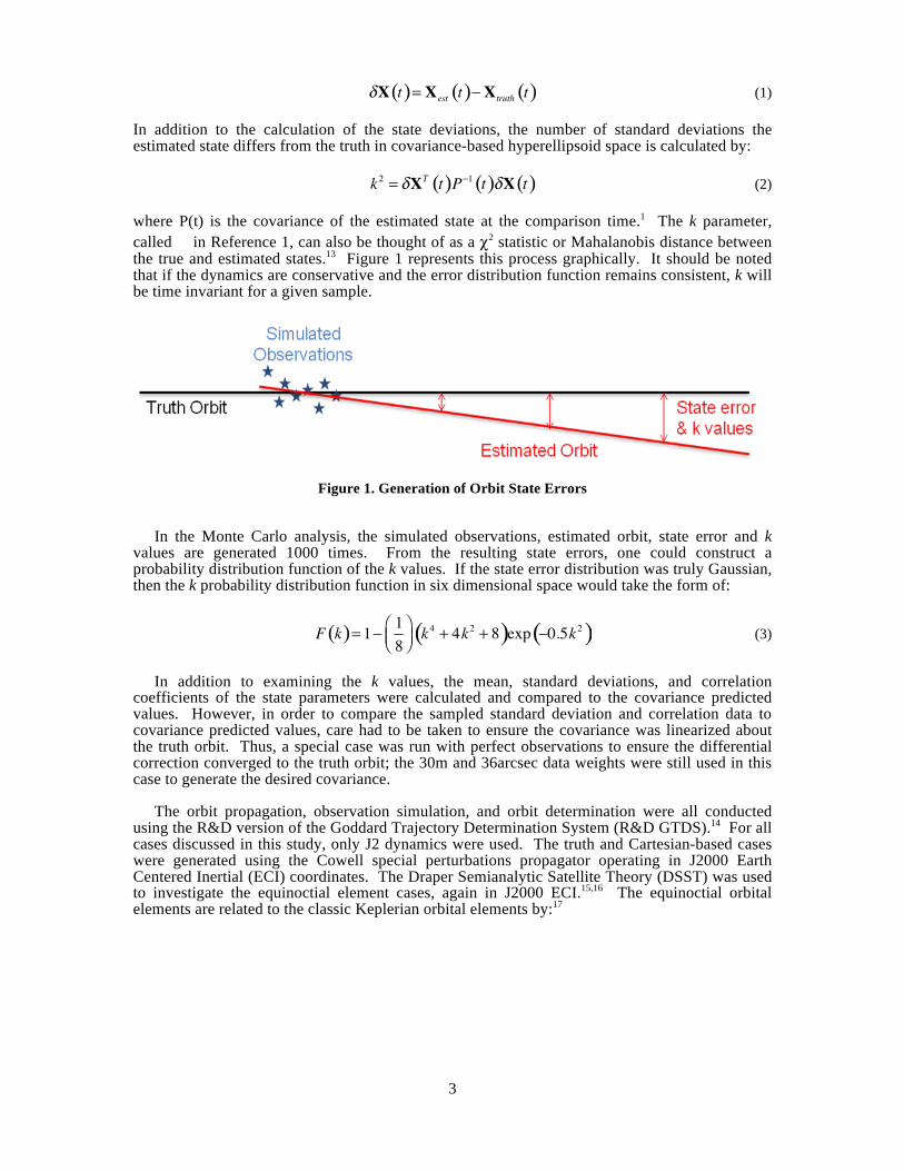
(1) In addition to the calculation of the state deviations, the number of standard deviations the estimated state differs from the truth in covariance-based hyperellipsoid space is calculated by: (2) where P(t) is the covariance of the estimated state at the comparison time.1 The k parameter, called � in Reference 1, can also be thought of as a χ2 statistic or Mahalanobis distance between the true and estimated states.13 Figure 1 represents this process graphically. It should be noted that if the dynamics are conservative and the error distribution function remains consistent, k will be time invariant for a given sample.

Figure 1. Generation of Orbit State Errors

In the Monte Carlo analysis, the simulated observations, estimated orbit, state error and k values are generated 1000 times. From the resulting state errors, one could construct a probability distribution function of the k values. If the state error distribution was truly Gaussian, then the k probability distribution function in six dimensional space would take the form of:

(3)

In addition to examining the k values, the mean, standard deviations, and correlation

coefficients of the state parameters were calculated and compared to the covariance predicted values. However, in order to compare the sampled standard deviation and correlation data to covariance predicted values, care had to be taken to ensure the covariance was linearized about the truth orbit. Thus, a special case was run with perfect observations to ensure the differential correction converged to the truth orbit; the 30m and 36arcsec data weights were still used in this case to generate the desired covariance.

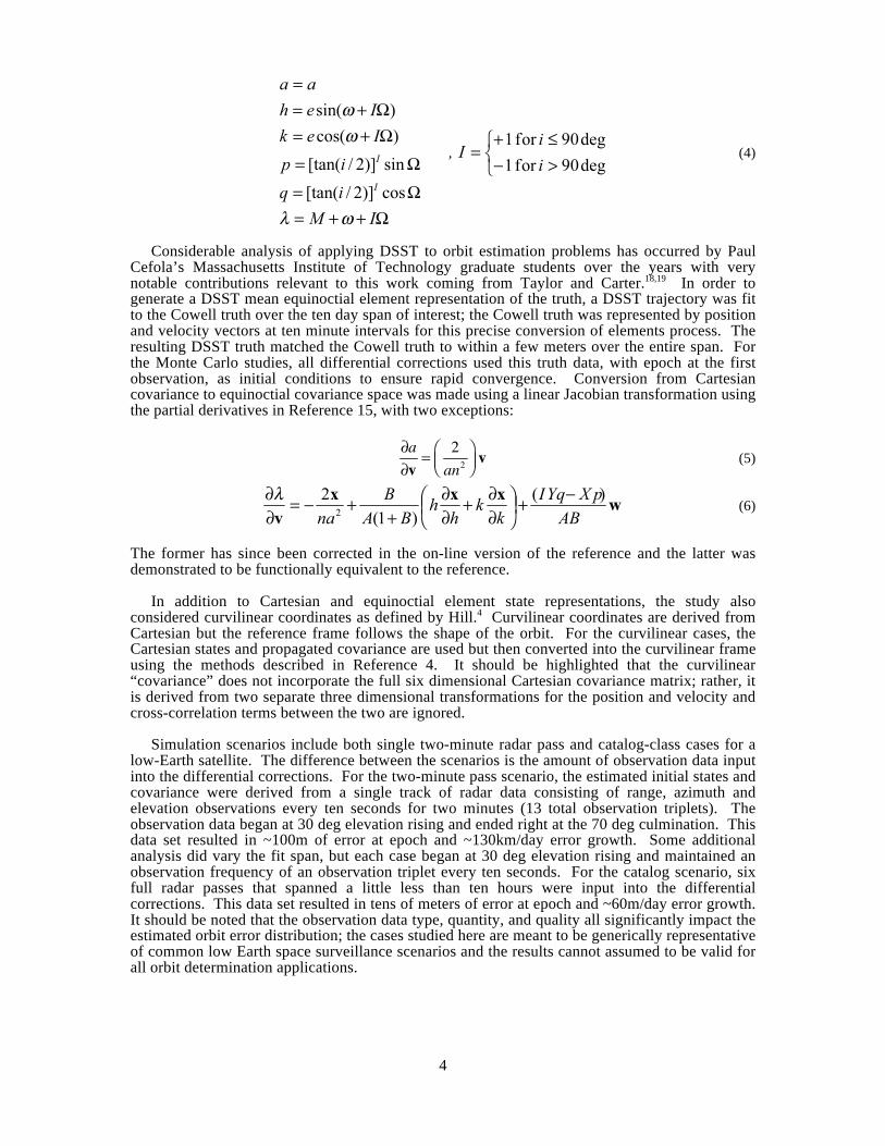
The orbit propagation, observation simulation, and orbit determination were all conducted using the R&D version of the Goddard Trajectory Determination System (R&D GTDS).14 For all cases discussed in this study, only J2 dynamics were used. The truth and Cartesian-based cases were generated using the Cowell special perturbations propagator operating in J2000 Earth Centered Inertial (ECI) coordinates. The Draper Semianalytic Satellite Theory (DSST) was used to investigate the equinoctial element cases, again in J2000 ECI.15,16 The equinoctial orbital elements are related to the classic Keplerian orbital elements by:17

4

, (4)

Considerable analysis of applying DSST to orbit estimation problems has occurred by Paul

Cefola’s Massachusetts Institute of Technology graduate students over the years with very notable contributions relevant to this work coming from Taylor and Carter.18,19 In order to generate a DSST mean equinoctial element representation of the truth, a DSST trajectory was fit to the Cowell truth over the ten day span of interest; the Cowell truth was represented by position and velocity vectors at ten minute intervals for this precise conversion of elements process. The resulting DSST truth matched the Cowell truth to within a few meters over the entire span. For the Monte Carlo studies, all differential corrections used this truth data, with epoch at the first observation, as initial conditions to ensure rapid convergence. Conversion from Cartesian covariance to equinoctial covariance space was made using a linear Jacobian transformation using the partial derivatives in Reference 15, with two exceptions:

(5)

(6)

The former has since been corrected in the on-line version of the reference and the latter was demonstrated to be functionally equivalent to the reference.

In addition to Cartesian and equinoctial element state representations, the study also considered curvilinear coordinates as defined by Hill.4 Curvilinear coordinates are derived from Cartesian but the reference frame follows the shape of the orbit. For the curvilinear cases, the Cartesian states and propagated covariance are used but then converted into the curvilinear frame using the methods described in Reference 4. It should be highlighted that the curvilinear “covariance” does not incorporate the full six dimensional Cartesian covariance matrix; rather, it is derived from two separate three dimensional transformations for the position and velocity and cross-correlation terms between the two are ignored.

Simulation scenarios include both single two-minute radar pass and catalog-class cases for a low-Earth satellite. The difference between the scenarios is the amount of observation data input into the differential corrections. For the two-minute pass scenario, the estimated initial states and covariance were derived from a single track of radar data consisting of range, azimuth and elevation observations every ten seconds for two minutes (13 total observation triplets). The observation data began at 30 deg elevation rising and ended right at the 70 deg culmination. This data set resulted in ~100m of error at epoch and ~130km/day error growth. Some additional analysis did vary the fit span, but each case began at 30 deg elevation rising and maintained an observation frequency of an observation triplet every ten seconds. For the catalog scenario, six full radar passes that spanned a little less than ten hours were input into the differential corrections. This data set resulted in tens of meters of error at epoch and ~60m/day error growth. It should be noted that the observation data type, quantity, and quality all significantly impact the estimated orbit error distribution; the cases studied here are meant to be generically representative of common low Earth space surveillance scenarios and the results cannot assumed to be valid for all orbit determination applications.

5

The R&D GTDS components of the simulations were wrapped using perl scripting language

and the runs were executed on the Maui High Performance Computing Center’s Mana system. RESULTS

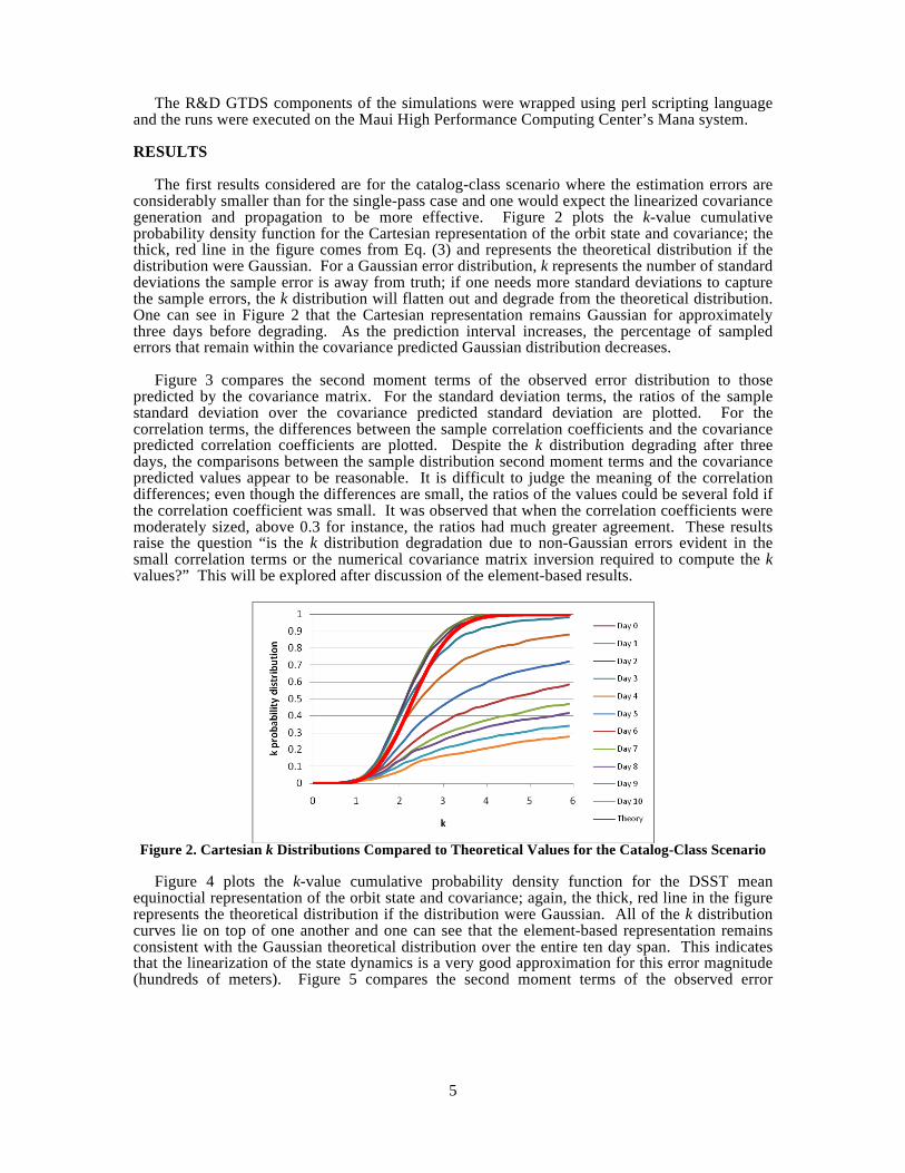
The first results considered are for the catalog-class scenario where the estimation errors are considerably smaller than for the single-pass case and one would expect the linearized covariance generation and propagation to be more effective. Figure 2 plots the k-value cumulative probability density function for the Cartesian representation of the orbit state and covariance; the thick, red line in the figure comes from Eq. (3) and represents the theoretical distribution if the distribution were Gaussian. For a Gaussian error distribution, k represents the number of standard deviations the sample error is away from truth; if one needs more standard deviations to capture the sample errors, the k distribution will flatten out and degrade from the theoretical distribution. One can see in Figure 2 that the Cartesian representation remains Gaussian for approximately three days before degrading. As the prediction interval increases, the percentage of sampled errors that remain within the covariance predicted Gaussian distribution decreases.

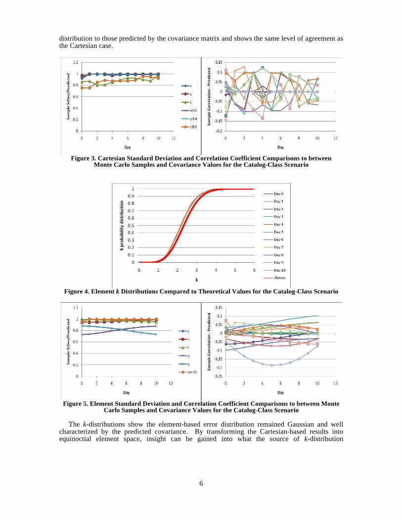
Figure 3 compares the second moment terms of the observed error distribution to those

predicted by the covariance matrix. For the standard deviation terms, the ratios of the sample standard deviation over the covariance predicted standard deviation are plotted. For the correlation terms, the differences between the sample correlation coefficients and the covariance predicted correlation coefficients are plotted. Despite the k distribution degrading after three days, the comparisons between the sample distribution second moment terms and the covariance predicted values appear to be reasonable. It is difficult to judge the meaning of the correlation differences; even though the differences are small, the ratios of the values could be several fold if the correlation coefficient was small. It was observed that when the correlation coefficients were moderately sized, above 0.3 for instance, the ratios had much greater agreement. These results raise the question “is the k distribution degradation due to non-Gaussian errors evident in the small correlation terms or the numerical covariance matrix inversion required to compute the k values?” This will be explored after discussion of the element-based results.

Figure 2. Cartesian k Distributions Compared to Theoretical Values for the Catalog-Class Scenario

Figure 4 plots the k-value cumulative probability density function for the DSST mean

equinoctial representation of the orbit state and covariance; again, the thick, red line in the figure represents the theoretical distribution if the distribution were Gaussian. All of the k distribution curves lie on top of one another and one can see that the element-based representation remains consistent with the Gaussian theoretical distribution over the entire ten day span. This indicates that the linearization of the state dynamics is a very good approximation for this error magnitude (hundreds of meters). Figure 5 compares the second moment terms of the observed error

6

distribution to those predicted by the covariance matrix and shows the same level of agreement as the Cartesian case.

Figure 3. Cartesian Standard Deviation and Correlation Coefficient Comparisons to between

Monte Carlo Samples and Covariance Values for the Catalog-Class Scenario

Figure 4. Element k Distributions Compared to Theoretical Values for the Catalog-Class Scenario

Figure 5. Element Standard Deviation and Correlation Coefficient Comparisons to between Monte

Carlo Samples and Covariance Values for the Catalog-Class Scenario

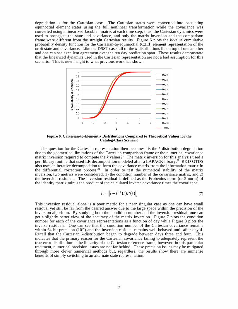
The k-distributions show the element-based error distribution remained Gaussian and well characterized by the predicted covariance. By transforming the Cartesian-based results into equinoctial element space, insight can be gained into what the source of k-distribution

7

degradation is for the Cartesian case. The Cartesian states were converted into osculating equinoctial element states using the full nonlinear transformation while the covariance was converted using a linearized Jacobian matrix at each time step; thus, the Cartesian dynamics were used to propagate the state and covariance, and only the matrix inversion and the comparison frame were different from the straight Cartesian results. Figure 6 plots the k-value cumulative probability density function for the Cartesian-to-equinoctial (C2El) element representation of the orbit state and covariance. Like the DSST case, all of the k-distributions lie on top of one another and one can see excellent agreement over the ten day prediction span. These results demonstrate that the linearized dynamics used in the Cartesian representation are not a bad assumption for this scenario. This is new insight to what previous work has shown.

Figure 6. Cartesian-to-Element k Distributions Compared to Theoretical Values for the

Catalog-Class Scenario

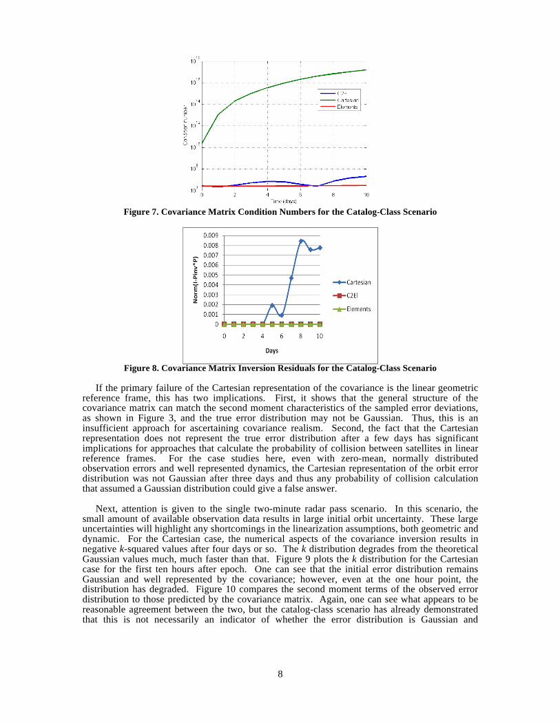
The question for the Cartesian representation then becomes “is the k distribution degradation due to the geometrical limitations of the Cartesian comparison frame or the numerical covariance matrix inversion required to compute the k values?” The matrix inversion for this analysis used a perl library routine that used LR decomposition modeled after a LAPACK library.20 R&D GTDS also uses an iterative decomposition to form the covariance matrix from the information matrix in the differential correction process.21 In order to test the numerical stability of the matrix inversion, two metrics were considered: 1) the condition number of the covariance matrix, and 2) the inversion residuals. The inversion residual is defined as the Frobenius norm (or 2-norm) of the identity matrix minus the product of the calculated inverse covariance times the covariance: (7) This inversion residual alone is a poor metric for a near singular case as one can have small residual yet still be far from the desired answer due to the large space within the precision of the inversion algorithm. By studying both the condition number and the inversion residual, one can get a slightly better view of the accuracy of the matrix inversion. Figure 7 plots the condition number for each of the covariance representations as a function of day while Figure 8 plots the inverse residuals. One can see that the condition number of the Cartesian covariance remains within 64-bit precision (1016) and the inversion residual remains well behaved until after day 4. Recall that the Cartesian k-distribution began to degrade between days three and four. This indicates that the primary reason for the Cartesian covariance failing to adequately represent the true error distribution is the linearity of the Cartesian reference frame; however, in this particular treatment, numerical precision issues are not far behind. These precision issues may be mitigated through more clever numerical methods but, regardless, the results show there are immense benefits of simply switching to an alternate state representation.

8

Figure 7. Covariance Matrix Condition Numbers for the Catalog-Class Scenario

Figure 8. Covariance Matrix Inversion Residuals for the Catalog-Class Scenario

If the primary failure of the Cartesian representation of the covariance is the linear geometric

reference frame, this has two implications. First, it shows that the general structure of the covariance matrix can match the second moment characteristics of the sampled error deviations, as shown in Figure 3, and the true error distribution may not be Gaussian. Thus, this is an insufficient approach for ascertaining covariance realism. Second, the fact that the Cartesian representation does not represent the true error distribution after a few days has significant implications for approaches that calculate the probability of collision between satellites in linear reference frames. For the case studies here, even with zero-mean, normally distributed observation errors and well represented dynamics, the Cartesian representation of the orbit error distribution was not Gaussian after three days and thus any probability of collision calculation that assumed a Gaussian distribution could give a false answer.

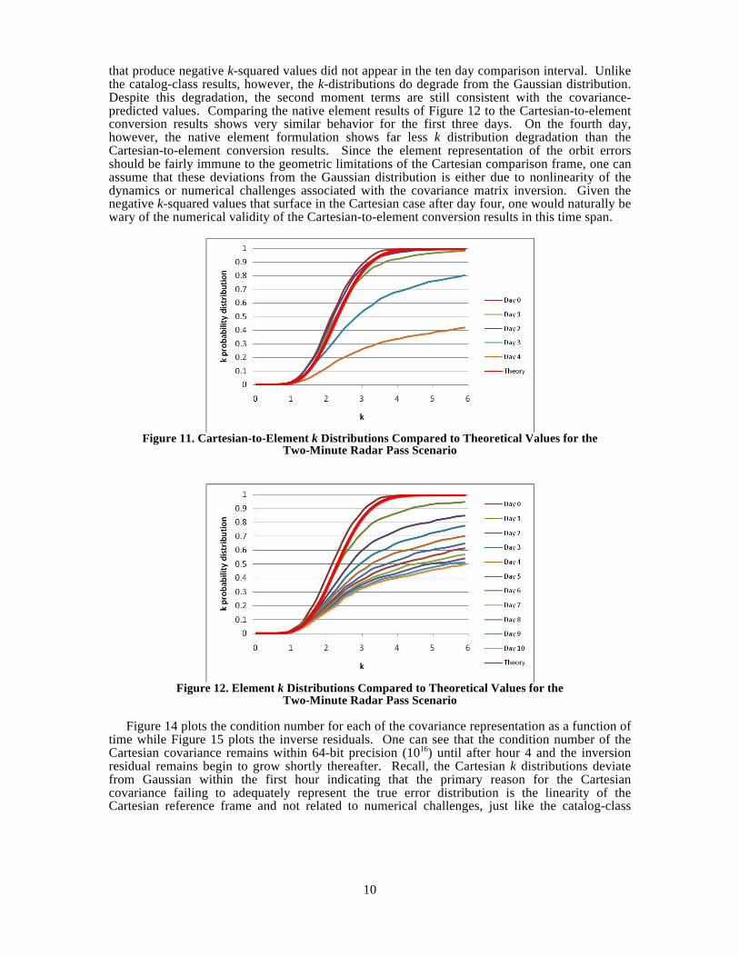
Next, attention is given to the single two-minute radar pass scenario. In this scenario, the small amount of available observation data results in large initial orbit uncertainty. These large uncertainties will highlight any shortcomings in the linearization assumptions, both geometric and dynamic. For the Cartesian case, the numerical aspects of the covariance inversion results in negative k-squared values after four days or so. The k distribution degrades from the theoretical Gaussian values much, much faster than that. Figure 9 plots the k distribution for the Cartesian case for the first ten hours after epoch. One can see that the initial error distribution remains Gaussian and well represented by the covariance; however, even at the one hour point, the distribution has degraded. Figure 10 compares the second moment terms of the observed error distribution to those predicted by the covariance matrix. Again, one can see what appears to be reasonable agreement between the two, but the catalog-class scenario has already demonstrated that this is not necessarily an indicator of whether the error distribution is Gaussian and

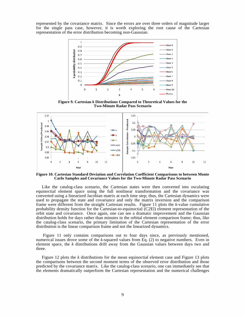
9

represented by the covariance matrix. Since the errors are over three orders of magnitude larger for the single pass case, however, it is worth exploring the root cause of the Cartesian representation of the error distribution becoming non-Gaussian.

Figure 9. Cartesian k Distributions Compared to Theoretical Values for the

Two-Minute Radar Pass Scenario

Figure 10. Cartesian Standard Deviation and Correlation Coefficient Comparisons to between Monte

Carlo Samples and Covariance Values for the Two-Minute Radar Pass Scenario

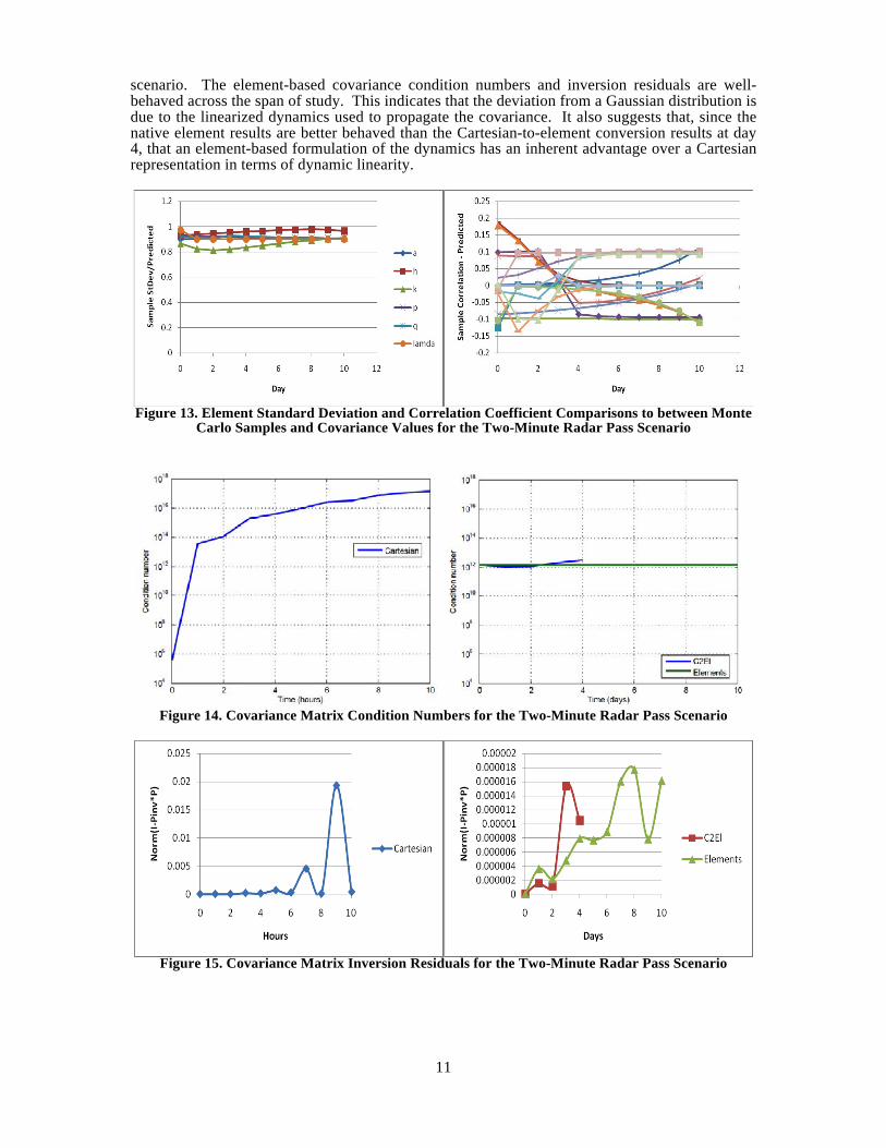
Like the catalog-class scenario, the Cartesian states were then converted into osculating equinoctial element space using the full nonlinear transformation and the covariance was converted using a linearized Jacobian matrix at each time step; thus, the Cartesian dynamics were used to propagate the state and covariance and only the matrix inversion and the comparison frame were different from the straight Cartesian results. Figure 11 plots the k-value cumulative probability density function for the Cartesian-to-equinoctial (C2El) element representation of the orbit state and covariance. Once again, one can see a dramatic improvement and the Gaussian distribution holds for days rather than minutes in the orbital element comparison frame; thus, like the catalog-class scenario, the primary limitation of the Cartesian representation of the error distribution is the linear comparison frame and not the linearized dynamics.

Figure 11 only contains comparisons out to four days since, as previously mentioned, numerical issues drove some of the k-squared values from Eq. (2) to negative numbers. Even in element space, the k distributions drift away from the Gaussian values between days two and three.

Figure 12 plots the k distributions for the mean equinoctial element case and Figure 13 plots the comparisons between the second moment terms of the observed error distribution and those predicted by the covariance matrix. Like the catalog-class scenario, one can immediately see that the elements dramatically outperform the Cartesian representation and the numerical challenges

10

that produce negative k-squared values did not appear in the ten day comparison interval. Unlike the catalog-class results, however, the k-distributions do degrade from the Gaussian distribution. Despite this degradation, the second moment terms are still consistent with the covariance-predicted values. Comparing the native element results of Figure 12 to the Cartesian-to-element conversion results shows very similar behavior for the first three days. On the fourth day, however, the native element formulation shows far less k distribution degradation than the Cartesian-to-element conversion results. Since the element representation of the orbit errors should be fairly immune to the geometric limitations of the Cartesian comparison frame, one can assume that these deviations from the Gaussian distribution is either due to nonlinearity of the dynamics or numerical challenges associated with the covariance matrix inversion. Given the negative k-squared values that surface in the Cartesian case after day four, one would naturally be wary of the numerical validity of the Cartesian-to-element conversion results in this time span.

Figure 11. Cartesian-to-Element k Distributions Compared to Theoretical Values for the

Two-Minute Radar Pass Scenario

Figure 12. Element k Distributions Compared to Theoretical Values for the

Two-Minute Radar Pass Scenario

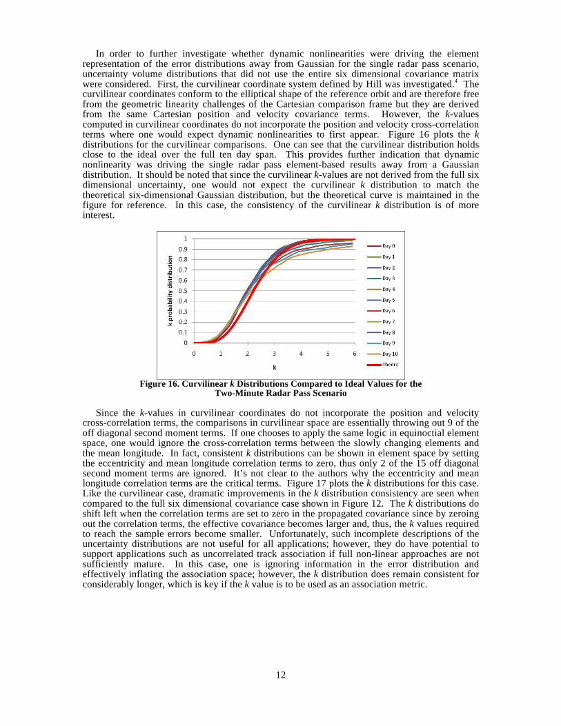
Figure 14 plots the condition number for each of the covariance representation as a function of time while Figure 15 plots the inverse residuals. One can see that the condition number of the Cartesian covariance remains within 64-bit precision (1016) until after hour 4 and the inversion residual remains begin to grow shortly thereafter. Recall, the Cartesian k distributions deviate from Gaussian within the first hour indicating that the primary reason for the Cartesian covariance failing to adequately represent the true error distribution is the linearity of the Cartesian reference frame and not related to numerical challenges, just like the catalog-class

11

scenario. The element-based covariance condition numbers and inversion residuals are well-behaved across the span of study. This indicates that the deviation from a Gaussian distribution is due to the linearized dynamics used to propagate the covariance. It also suggests that, since the native element results are better behaved than the Cartesian-to-element conversion results at day 4, that an element-based formulation of the dynamics has an inherent advantage over a Cartesian representation in terms of dynamic linearity.

Figure 13. Element Standard Deviation and Correlation Coefficient Comparisons to between Monte

Carlo Samples and Covariance Values for the Two-Minute Radar Pass Scenario

Figure 14. Covariance Matrix Condition Numbers for the Two-Minute Radar Pass Scenario

Figure 15. Covariance Matrix Inversion Residuals for the Two-Minute Radar Pass Scenario

12

In order to further investigate whether dynamic nonlinearities were driving the element representation of the error distributions away from Gaussian for the single radar pass scenario, uncertainty volume distributions that did not use the entire six dimensional covariance matrix were considered. First, the curvilinear coordinate system defined by Hill was investigated.4 The curvilinear coordinates conform to the elliptical shape of the reference orbit and are therefore free from the geometric linearity challenges of the Cartesian comparison frame but they are derived from the same Cartesian position and velocity covariance terms. However, the k-values computed in curvilinear coordinates do not incorporate the position and velocity cross-correlation terms where one would expect dynamic nonlinearities to first appear. Figure 16 plots the k distributions for the curvilinear comparisons. One can see that the curvilinear distribution holds close to the ideal over the full ten day span. This provides further indication that dynamic nonlinearity was driving the single radar pass element-based results away from a Gaussian distribution. It should be noted that since the curvilinear k-values are not derived from the full six dimensional uncertainty, one would not expect the curvilinear k distribution to match the theoretical six-dimensional Gaussian distribution, but the theoretical curve is maintained in the figure for reference. In this case, the consistency of the curvilinear k distribution is of more interest.

Figure 16. Curvilinear k Distributions Compared to Ideal Values for the

Two-Minute Radar Pass Scenario

Since the k-values in curvilinear coordinates do not incorporate the position and velocity cross-correlation terms, the comparisons in curvilinear space are essentially throwing out 9 of the off diagonal second moment terms. If one chooses to apply the same logic in equinoctial element space, one would ignore the cross-correlation terms between the slowly changing elements and the mean longitude. In fact, consistent k distributions can be shown in element space by setting the eccentricity and mean longitude correlation terms to zero, thus only 2 of the 15 off diagonal second moment terms are ignored. It’s not clear to the authors why the eccentricity and mean longitude correlation terms are the critical terms. Figure 17 plots the k distributions for this case. Like the curvilinear case, dramatic improvements in the k distribution consistency are seen when compared to the full six dimensional covariance case shown in Figure 12. The k distributions do shift left when the correlation terms are set to zero in the propagated covariance since by zeroing out the correlation terms, the effective covariance becomes larger and, thus, the k values required to reach the sample errors become smaller. Unfortunately, such incomplete descriptions of the uncertainty distributions are not useful for all applications; however, they do have potential to support applications such as uncorrelated track association if full non-linear approaches are not sufficiently mature. In this case, one is ignoring information in the error distribution and effectively inflating the association space; however, the k distribution does remain consistent for considerably longer, which is key if the k value is to be used as an association metric.

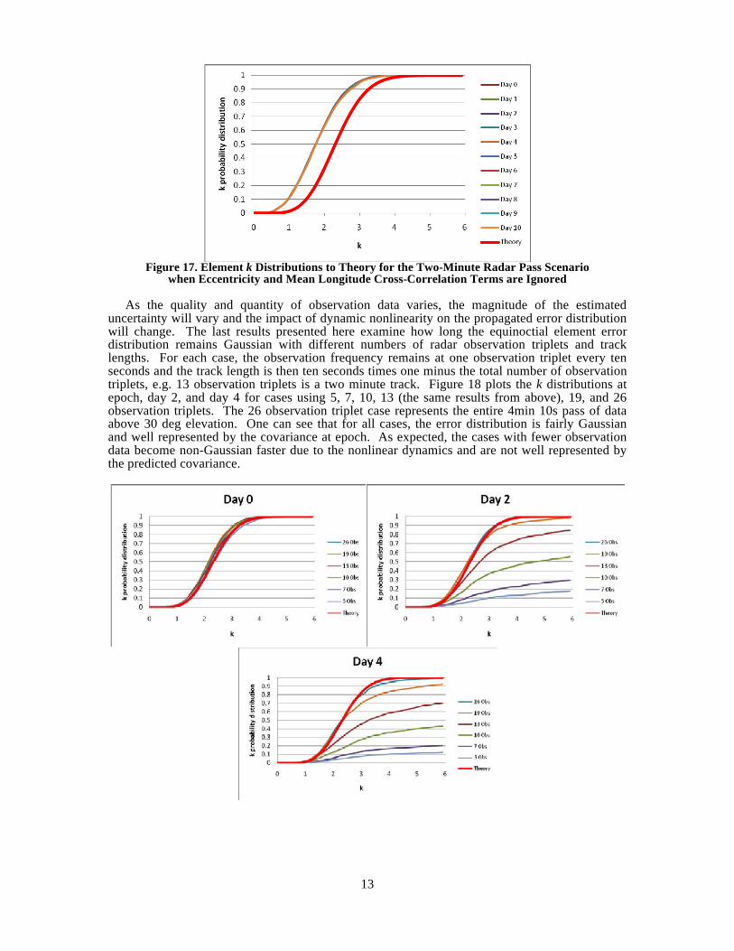
13

Figure 17. Element k Distributions to Theory for the Two-Minute Radar Pass Scenario

when Eccentricity and Mean Longitude Cross-Correlation Terms are Ignored

As the quality and quantity of observation data varies, the magnitude of the estimated uncertainty will vary and the impact of dynamic nonlinearity on the propagated error distribution will change. The last results presented here examine how long the equinoctial element error distribution remains Gaussian with different numbers of radar observation triplets and track lengths. For each case, the observation frequency remains at one observation triplet every ten seconds and the track length is then ten seconds times one minus the total number of observation triplets, e.g. 13 observation triplets is a two minute track. Figure 18 plots the k distributions at epoch, day 2, and day 4 for cases using 5, 7, 10, 13 (the same results from above), 19, and 26 observation triplets. The 26 observation triplet case represents the entire 4min 10s pass of data above 30 deg elevation. One can see that for all cases, the error distribution is fairly Gaussian and well represented by the covariance at epoch. As expected, the cases with fewer observation data become non-Gaussian faster due to the nonlinear dynamics and are not well represented by the predicted covariance.

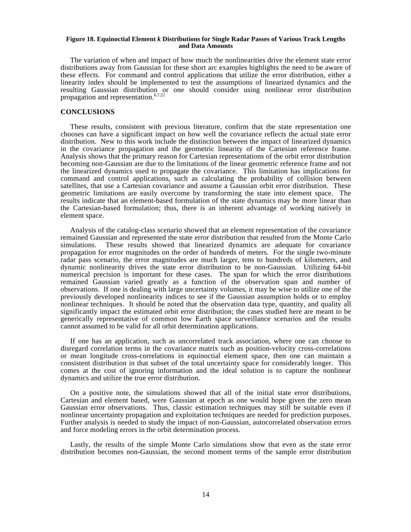
14

Figure 18. Equinoctial Element k Distributions for Single Radar Passes of Various Track Lengths and Data Amounts

The variation of when and impact of how much the nonlinearities drive the element state error

distributions away from Gaussian for these short arc examples highlights the need to be aware of these effects. For command and control applications that utilize the error distribution, either a linearity index should be implemented to test the assumptions of linearized dynamics and the resulting Gaussian distribution or one should consider using nonlinear error distribution propagation and representation.6,7,22 CONCLUSIONS

These results, consistent with previous literature, confirm that the state representation one chooses can have a significant impact on how well the covariance reflects the actual state error distribution. New to this work include the distinction between the impact of linearized dynamics in the covariance propagation and the geometric linearity of the Cartesian reference frame. Analysis shows that the primary reason for Cartesian representations of the orbit error distribution becoming non-Gaussian are due to the limitations of the linear geometric reference frame and not the linearized dynamics used to propagate the covariance. This limitation has implications for command and control applications, such as calculating the probability of collision between satellites, that use a Cartesian covariance and assume a Gaussian orbit error distribution. These geometric limitations are easily overcome by transforming the state into element space. The results indicate that an element-based formulation of the state dynamics may be more linear than the Cartesian-based formulation; thus, there is an inherent advantage of working natively in element space.

Analysis of the catalog-class scenario showed that an element representation of the covariance remained Gaussian and represented the state error distribution that resulted from the Monte Carlo simulations. These results showed that linearized dynamics are adequate for covariance propagation for error magnitudes on the order of hundreds of meters. For the single two-minute radar pass scenario, the error magnitudes are much larger, tens to hundreds of kilometers, and dynamic nonlinearity drives the state error distribution to be non-Gaussian. Utilizing 64-bit numerical precision is important for these cases. The span for which the error distributions remained Gaussian varied greatly as a function of the observation span and number of observations. If one is dealing with large uncertainty volumes, it may be wise to utilize one of the previously developed nonlinearity indices to see if the Gaussian assumption holds or to employ nonlinear techniques. It should be noted that the observation data type, quantity, and quality all significantly impact the estimated orbit error distribution; the cases studied here are meant to be generically representative of common low Earth space surveillance scenarios and the results cannot assumed to be valid for all orbit determination applications.

If one has an application, such as uncorrelated track association, where one can choose to disregard correlation terms in the covariance matrix such as position-velocity cross-correlations or mean longitude cross-correlations in equinoctial element space, then one can maintain a consistent distribution in that subset of the total uncertainty space for considerably longer. This comes at the cost of ignoring information and the ideal solution is to capture the nonlinear dynamics and utilize the true error distribution.

On a positive note, the simulations showed that all of the initial state error distributions, Cartesian and element based, were Gaussian at epoch as one would hope given the zero mean Gaussian error observations. Thus, classic estimation techniques may still be suitable even if nonlinear uncertainty propagation and exploitation techniques are needed for prediction purposes. Further analysis is needed to study the impact of non-Gaussian, autocorrelated observation errors and force modeling errors in the orbit determination process.

Lastly, the results of the simple Monte Carlo simulations show that even as the state error distribution becomes non-Gaussian, the second moment terms of the sample error distribution

15

may still appear consistent with the terms in the covariance matrix. Therefore, calculating the standard deviation and correlation terms of the sampled state error distribution and finding agreement with the covariance matrix is an insufficient test of covariance realism and the Gaussian nature of the true error distribution. Even if the covariance reflects the second moment terms of the true error distribution, it does not provide insight into whether higher moments are needed. ACKNOWLEDGMENTS

The authors gratefully acknowledge the support of the Department of Defense High Performance Computing Modernization Program office through the High Performance Computing Software Applications Institute for Space Situation Awareness and Summer Cadet Research Program. We thank the staff of the Maui High Performance Computing Center for their assistance with the simulations. Cadet Sukut’s efforts were supported by the U.S. Air Force Academy and advisor Scott Dahlke. Lastly, the authors thank Moriba Jah of the Air Force Research Laboratory, Don Danielson of the Naval Postgraduate School, and Paul Cefola for discussions involving this research. REFERENCES [1] Tapley, B. D., Schutz, B. E., and Born, G. H., Statistical Orbit Determination, Elsevier Academic Press,

Burlington, MA, 2004. [2] Hill, K., et al, “Covariance-based Network Tasking of Optical Sensors,” AAS 10-150, AAS/AIAA Space Flight

Mechanics Meeting, San Diego, CA, 14-17 Feb 2010. [3] Alfriend, K. T., “A Dynamic Algorithm for Processing Uncorrelated Tracks," AAS 97-607, AAS/AIAA

Astrodynamics Specialist Conference, Sun Valley, Idaho, Aug. 4-7, 1997 [4] Hill, K., K.T. Alfriend, C. Sabol, “Covariance-based Uncorrelated Track Association,” AIAA 2008-7211,

AIAA/AAS Astrodynamics Specialist Conference, Honolulu, HI, August 2008. [5] Chan, F. K., Spacecraft Collision Probability, published jointly by The Aerospace Corporation (El Segundo,

California) and the American Institute of Aeronautics and Astronautics, Inc. (Reston, Virginia), 2008. [6] Junkins, J., Akella, M., and Alfriend, K., “Non-Gaussian Error Propagation in Orbit Mechanics,” Journal of the

Astronautical Sciences, Vol. 44, No. 4, 1996, pp. 541–563. [7] Park, R. S. and Scheeres, D. J., “Nonlinear Mapping of Gaussian Statistics: Theory and Applications to Spacecraft

Trajectory Design," Journal of Guidance, Control, and Dynamics, Vol. 29, No. 6, 2006, pp. 1367-1375. [8] Vallado, D. A., J. H. Seago, “Covariance Realism,” AAS/AIAA Astrodynamics Specialist Conference, Pittsburgh,

PA, August 9-13, 2009, AAS 09-304. [9] Kelecy, T., M. Jah, “Analysis of Orbit Predictions to Thermal Emissions Acceleration Modeling for High Area-to-

Mass Ratio (HMR) Objects,” Air Force Research Laboratory Technical Report, AFRL-RD-PS-TP-2009-1021. [10] Denham, W., S. Pines, “Sequential Estimation when Measurement Function Nonlinearity is Comparable to

Measurement Error,” AIAA Journal, VOL. 4, NO. 6, JUNE 1966 [11] Press, W. H., S. A. Teukolsky, W. T. Vetterling, B. P. Flannery, Numerical Recipes in FORTRAN, Second

Edition, Cambridge University Press, New York, NY, 1992. [12] Vallado, D. and McClain, W., Fundamentals of Astrodynamics and Applications, Microcosm Press, El Segundo,

CA, 3rd ed., 2007. [13] Mahalanobis, P. C., “On the Generalized Distance in Statistics," Proceedings of the National Institute of Sciences

of India, Vol. 2, 1936, pp. 49-55.

16

[14] Computer Sciences Corporation and NASA/GSFC Systems Development and Analysis Branch (Editors),

Research and Development Goddard Trajectory Determination System (R&D GTDS) User’s Guide, July, 1978. [15] Danielson, D. A., et al, Semianalytic Satellite Theory, Technical Report NPS-MA-95-002, Naval Postgraduate

School, 1995. [16] Sabol, C., Carter, S., Bir, M., “Analysis of Preselected Orbit Generator Options for the Draper Semianalytic

Satellite Theory”, AIAA/AAS Astrodynamics Specialist Conference, Denver, CO, August 14-17, 2000, AIAA 2000-4231.

[17] Broucke, R. A. and Cefola, P. J., “On the Equinoctial Orbit Elements," Celestial Mechanics, Vol. 5, No. 3, 1972,

pp. 303-310. [18] Taylor, S., Semianalytic Satellite Theory and Sequential Estimation, Master of Science Thesis, Massachusetts

Institute of Technology, 1982. [19] Carter, S., Precision Orbit Determination from GPS Receiver Navigation Solutions, Master of Science Thesis,

Massachusetts Institute of Technology, 1996. [20] Anderson, E., et al, LAPACK Users’s Guide, Third Edition, Society for Industrial and Applied Mathematics,

Philadelphia, PA, 1999. [21] Computer Sciences Corp. and NASA Goddard Space Flight Center (Editors), GTDS Mathematical Theory

Revision 1¸Contract NAS 5-31500, Task 213, July 1989. [22] Giza, D., Singla, P., Jah, M, “An Approach for Nonlinear Uncertainty Propagation: Application to Orbital

Mechanics,” AIAA-2009-6082, 2009 AIAA Guidance, Navigation, and Control Conference, Chicago, Illinois, August 10-13, 2009.