f

Linearit,y-Preserving Limit,ers on Irregular Grids

Marsha Berger Michael -4ftosmis Scott _hl urman

Moffett Field, CA 94035 Courant Inst it ut e NASA Ames ELORET/NASA Ames

Xew York, h i 10012 MofFett Field, CA 94035 berger@cims. nyu. edu afiosmis@nas. nasa.gov smurman@nas. nasa.gov

Abstract

This paper examines the behavior of flux and slope limiters on non-uniform grids in multiple dimensions. We note that on non-uniform grids the scalar formulation in standard use today sacrifices k-exactness, even for linear solutions, impacting both accuracy and convergence. We rewrite some well-known limiters in a n way to highlight their underlying symmetry, and use this to examine both traditional and novel limiter formulations. A consistent method of handling stretched meshes is developed, as is a new directional formulation in multiple dimensions for irregular grids. Results are presented demonstrating improved accuracy and convergence using a combination of model problems and complex three-dimensional examples.

1 Introduction

For many finite-difference or finite-volume computations with discontinuous solutions lim- iters are a necessary evil. On one hand they suppress oscillations and maintain monotone solutions. On the other hand, they reduce accuracy and can hamper convergence to steady state [a]. Limiters can be difficult to extend to multidimensional unstructured grids, and they do not degenerate gracefully on distorted grids. Other problems can include limiter chatter, rattling in near-constant portions of the flow field, and additional convergence problems with Newton’s method for non-smooth limiters [13]. These problems can occur on both structured and unstructured grids, for both flux and slope-limiter formulations.

Most of the research on limiters has been in .one space dimension: where a reliable thecry &sts [63: There is suhst.mtia.lly less litemtiire on extensions to two or more dimen- sions, where theory is lacking. On multi-dimensional structured grids, limiters are typically applied independently in each coordinate direction, which works well in practice. On un- structured grids most codes use a scalar limiter, where the gradient is reduced by the same scalar fraction regardless of direction [3]. There is almost no discussion on the application of limiters to irregular or non-uniform grids, although nearly all meshes on real geome- tries fall into this category (some recent exceptions however are [7, 91). The purpose of this paper is to develop limiters that preserve monotonicity, are exact for linear solutions (called k-exactness for k = l ) , and have good convergence properties on non-smooth grids. We illustrate their performance with examples computed on multi-level Cartesian grids with embedded boundaries. These grids make a good testbed, since they include large portions

1

https://ntrs.nasa.gov/search.jsp?R=20040086828 2020-06-06T03:31:35+00:00Z

t

of regular uniform grid cells, mesh interfaces with 2:l mesh stretching, as weii as generai irregular polyhedra at the embedded boundaries.

In the rest of this section we briefly summarize some relevant. parts of the literature. Section 2 presents some problems with limiters in common use today, which may not be well-known. Section 3 discusses a solution to the problem of limiters on stretched meshes. Generalizatioas of one diixensiod limiters for multi-dimer,sior,al irregular grids are pre- sented in section 4. Computational results using both model problems and a variety of 3D test cases are presented in section 5.

1.1 Background

The most common framework for looking at limiters was systematized by Sweby [12], using the flux formulation. By analogy with Flux Corrected Transport [14], one writes a second- order scheme a s a first-order scheme plus a limited anti-diffusive flux, shown here for the case of linear advection ut + uu, = 0 , as

U?" = 'Up - x ( U i - 7Li-1) - ('$iFi+1/2 - '$i-IFi-1/2)

where the flux Ft+lp = iX(1 - X ) ( U , + ~ - ui). Here the &'s are the flux limiters, and

Define the ratio R of forward to backward differences in the solution (note that R is the A x .

inverse of Sweby's r ) as

By choosing gi = $(Ri) properly, a total-variation-diminishing (TVD) scheme can be achieved. Sweby the3 derives the well-known result

This is often expressed graphically for the different possible limiters using the Sweby diagram of figure l(a): choosing + in the shaded region leads to a second-order TVD solution. An important point to note is that for second order accuracy away from extrema, the limiter must satisfy

$(1) = 1.

In other words, the method should not do any limiting when the solution is a linear function. AISG $ must be symmetric,

although this symmetry may not be immediately apparent in figure l(b). Later we will rewrite the limiters in a more transparently symmetric form. All the limiters below satisfy

2

Fliix Limiters

2 n

W d 3

1

1

Figure 1: (a) Second order TVD region from 1121. (b) Common flux limiters $ from eq. (5).

the symmetry relation (2). Limiters of interest, in order of increasing dissipation, are

(super bee) gsb(R) = minmod[max(l, R), 2,2R] ( 3 ) 1 4R 4

(Barth - Jespersen) $BJ(R) = S(R + 1) min[min(l, -), min(1, -)] (4) R + l R + l

R 2 + R (van Albada) $VA(R) =

( 5 )

(6)

(minmod) gmm(R) = max{0, min(1, R)) (7)

The superbee limiter follows the boundary of the TVD region, and is included in figure l(b) for reference. The superbee and Barth-Jespersen limiters are the most compressive, and are known to turn smooth waves into square waves. In multiple dimensions their overly compressive nature may lead to staircasing of discontinuities on non-aligned grids.

Spekreijse [Ill shows the equivalence of flux limiting with slope limiting, which is more natural for finite volume schemes in REP form [5 ] : Reconstruct the solution from its cell averages, Evolve the reconstructed solution from time t, to tn+l, and Project the solution back onto the grid to update the integral cell averages at the new time. We can see this by compuring stares in the iiux form for linear advection, usiiig ciie one-sided diEeieiie5 fioIii the Fromm scheme. Computing the states at the cell interfaces we get

(8)

(9)

L 1

R 1 u,+1/2 = 212 t #(R,) (YZ - %-1)

Y

u,-1/2 = - S W / R % ) (%+1 - u z )

where u$1/3 is the left state at the right edge, etc. By requiring that this be equivalent to limiting a single reconstructed gradient at cell i, here the central difference (u2+1 -uz-1)/2h,

3

, ...

i

we get

Slope Limiters

n 1 "0 1 2 3 4

R

Figure 2: Common limiters in slope form from eq. (14)

Thus abng with using eq. (2), we get the relationship betweer? a flux limiter 7 ) and a slope limiter

R f l 2 $(R) = 4(R)(-).

Whereas flux limiters satisfy 0 5 $(R) _< 2, a slope limiter satisfies 0 5 4(R) 5 1. Slope limiters make the reconstruction step easy, by writing the reconstructed function U, (x) in cell i as UZ(x) = u, + +(R,)Vu,(z - x,), where u, is the cell average. Note that for any limiter $ satisfying eq. ( 2 ) , 4 satisfies the slope form of the symmetry condition

(12) 1

#?) = +q. Figure 2 shows the behavior of the same collection of limiters as figure 1 but this time

in their slope form. The common limiters in slope form are:

~ B J ( R ) = max(0, min(2R, l j , min(R, 2 ) ) (13)

(14) 4VL(R) =

(15) 4V.4(R) = -

(16)

4R ( R + 1)2

2R R2 + 1

2R 2 dmm(R) = max{O,min(- l + R ' l + R -I}

4

1.2 Symmetric View of Limiters

While slope limiters of the form in figure 2 are helpful, we briefly digress to p,reserit a 1m.m

intuitive way to graph the slope limiters. In figure 3 the independent variable f is the fraction u, - uZp1 of the u-hole jump uZL1 - u,-1. This form has the added benefit that we c m :mre easily see the beh2vior of the limiter fer larue 0 R.

Let the undivided differences A- = u, - u,-l, and A+ = uZI1 - u,, so that A, = u,+1 - u,-1 = A+ + A_. The fraction f = A-/A, gives a symmetric view of the slope limiters as f ranges from 0 to 1. The symmetry is more apparent since the limiter can be plotted as a function of A- or A+, and the function is symmetric about f = 1/2. It also becomes obvious that it is the neighbor of u, with the larger jump, either u,+1 or u,-1 that causes the limiting of uz’s slope, since it is thzs jump that would cause the overshoot at the other neighbor’s face. In these variables the common limiters become

7rn-

A, 4 . = sin(-) san

3 Slope Limiters in Symmetric Form

r I I 1

0.6 e

BarthJespersen van Leer sin lim

0.4

0.2 van Albada -

I rninrnod I

0.2 0.4 0.6 0.8 1 0: 0

f

r\ I

I I

I I I

IA c

I A T ’ *

I

I I

I I

I

I A +

v

u . 1- 1 U .

1 U.

I+ 1

Figure 3: (a) Symmetric form of slope limiters. (b) Cell averages corresponding to the limiters. When ui is exactly in the middle, the data is linear, f = .5, and the limiter is 1.

This symmetric form also makes it easy to devise new limiters. For example, inciuded

5

in figure 3(a) is a new sin limiter, defined by

) = cos(7r) sin( ___ -7i 1 7 i L T ( & - A+) AC 0, &

$sin(R) = sin(-) = sin(

L l C

This limiter is continuously differentiable, does not limit linear data, satisfies the symmetry property (12), and falls between the van Leer and van Albada limiters in terms of dissipation.

1.3 Multi-dimensional Formulations

On structured grids in two space dimensions Spekreijse limits each coordinate direction separately and the scheme preserves monotonicity at steady state. However Saltzman [lo] shows that for the second-order time-accurate MUSCL scheme in two dimensions, a larger neighborhood of values, illustrated in two dimensions in figure 4, needs to be included in the limiter for strict monotonicity of the time-dependent solution. He defines the new Benjamin limiter by extending Barth-Jespersen (also called the limited monotonicized cen- tral differences) to include corner coupling. A one-dimensional geometric interpretation of Barth-Jespersen is that the central difference cannot exceed twice the forward or backward differences at that cell. (From this it follows that the reconstructed value at the face does not exceed the neighbor’s cell-centered value). In two dimensions, the central difference must also be checked against the forward and backward differences of neighboring rows and columns to ensure there are no new maxima at the next time step. In Saltzman’s notation, but simplified here by assuming all gradients are positive, the limited gradient in the 5

direction can be written

Similarly, the limited y gradient is either the central difference in the j direction, or the minimum of twice the forward or backward difference in any neighboring column in that direction. This limiter has been found to be overly diffusive for many applications, but we will use elements reminiscent of it later in devising a limiter for cut cells.

Although limiters can be too dissipative they can also be too compressive, a wdl-ho-i~n pro’uiein r‘or e~a,~;rnpie w i i l i ilit: supel bee Gi- Eaith-Jaspaiseii liiiiiteis. Iii PFX, t l i ~ Eligki order reconstruction scheme of [4], this was handled by explicitly adding second difference dissipation at strong shocks in both the normal and the tangential direction. However one of our goals in section 4 will be to devise a more dissipative limiter to automatically accomplish this 011 irregu!ar grids.

2 Problems with Limiters

Despite the simple framework sketched in the previous section, the fact remains that the most common situations found in practice are more complex. Little work appears in the literature on applying limiters to irregular meshes in one or more dimensions. This includes

6

Figure 4: Stencil for the Benjamin limiter of eq. (18) for two-dimensional time-dependent problems. The gradient computed at i, j is compared with the forward differences (in green) and the backward differences (in purple) for the limiting in the x direction (a), and similarly for the y direction (b).

their application on unstructured meshes, although these grids are now nearly as common as their structured counterparts. In this section we illustrate some problems with limiters that are either not well known or ignored since practical solutions are not available.

2.1 Stretched Meshes

W-hen the grid is unstructured or irregular, a common procedure to approximate the gradient &t c& i is to use a Iez t sqiix-es lit to the solution iil neighboriiig cdIs [ 3 ] . In general this gives a first-order accurate approximation, and for linear data it is exact, even on distorted meshes. However the limiting procedure can destroy this property.

We illustrate this in one-dimension using three unequally spaced adjacent grid cells. The least squares gradient approximation at cell i is

where h+ = zi+l - zi, h- = xi - zi-1, D+ui = (ui+l - ui)/h+, etc. Note that the least squares gradient in eqn. (19) is a convex combination of the forward and backward differences computed on the irregular mesh. If the mesh is uniform, h+ = h-, the weights become 1/2 each, and we recover the familiar second-order first derivative stencil

On a non-uniform mesh a second order accurate gradient approximation is of course possible, but it does not minimize the least squares error of the linear fit. The second order non- uniform approximation is a linear combination with different weights, Vuz = =D+uz +

Consider the one dimensional stretched mesh of figure 5, where the cell size of u, is h. In the left figure the mesh is locally irregular, and the cell size of uz+l is h/2 In the figure on the right: the mesh has a constant stretching ratio of 2. If eq. (1) is applied to linear data with slope s ,

h i

h- - u - U , . h++h-

U , i l - 21% - s . (5 ,+1 - zz) - 3/4h 3 - - - 4 '

R= U , - ~ ~ - 1 (x% - ~ 2 - 1 ) h

7

Figure 5: The left mesh has a mesh refinement interface; the mesh on the right has a constant stretching ratio. The ratio of the difference R = - is 3/4 in (a) or 1 /2 in (b). For linear data a ratio of 1.0 is expected by the uncorrected slope or flux limiter forms in eq. (14) or (5).

where the cell average value u, is taken to be located at the cell center 5,. On a uniform grid this ratio would be 1 but on a stretched mesh it isn't, so most of the limiters (except Barth-Jespersen or superbee) will be activated. For example, the van Leer limiter of (14) gives a limiter value of 6/7 when R = 3/4. For the grid in figure 5(b) R=1/2, and the limiter value will be 2/3. The Barth-Jespersen limiter, which has the geometric interpretation that the reconstruction at the ceii edge should not exceed tlie cell centered due of the adjacefit cell does not require limiting on stretched meshes for any stretching ratio.

Figure 6: In a11 three examples, Iinear data is not preserved by standard limiters. Let the line between cell centers A and B also be the level lines of the solution. The flux evaluation and solution limiting occurs at point C, which is not on the line. Point C will have an overshoot, and the eziict gradient which was reccnstructed at A and B will be limited.

This limiting of linear solutions occurs often in higher dimensions, and is responsible for some loss of accuracy. The limiting is occurring iiot because of extrema or discmtinuities, but simply because of the mesh stretching. Figure 6 shows three situations where this can occur. In each case, let the linear data be such that points A and B are equal. Point C will then'be an extremum when compared to the cell averages, and the gradients at both A and

8

B Lviii be iimired. This happens regardless of which iirriiter is used, sirice all iimiters will see C as a new extremum. On smoothly varying triangular grids where the median dual is approximated with the centroidal dual, the midpoint of the edge is only O(h') from the point on the line bemeen the two neighbors, so this is not likely to be noticeable. On the other hand, the use of scalar limiters in multiple dimensions will exacerbate this problem.

2.2 Face-based Limiters

One idea that has been previously suggested to reduce the dissipation from limiters is to apply them on a face-by-face basis. If one neighbor causes an adjacent cell to limit its gradient, the limiter would only be applied on its common face - that is, on one side of the reconstruction. The neighbor on the other side might allow some or all of the gradient to be used on the face it shares with the same cell. This can be thought of as a generalization of the geometric interpretation of the Barth-Jespersen limiter. Note that this limiting procedure does not preserve the mean of the reconstruction. Face-based limiting was shown not to work well in practice in [2]. Here we explain this by showing that this approach does not preserve monotonicity.

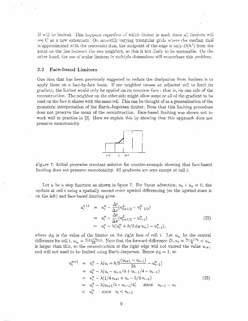
Figure 7: Initial piecewise constant solution for counter-example showing that face-based limiting does not preserve monotonicity. All gradients are zero except at cell i.

Let u be a step function as shown in figure 7. For linear advection, ut + u, = 0, the update at cell i using a spatially second order upwind differencing (so the upwind state is on the left) and face-based limiting gives

where d~ is the value of the limiter on the right face of cell i. Let uz, be the central difference for cell i, uz, = . Note that the forward difference D+uz = ___ h < u'b

is larger than this, so the reconstruction at the right edge will not exceed the value u,+1 and will not need to be limited using Barth-Jespersen. Hence d~ = 1, so

%+1 -ut- 1 &+l-% 2h

9

In other words, there will be an undershoot at zli at the next time step. As chis exampie shows, the face with the largest change in the solution is responsible for limiting at the other face. This does not occur with face-based limiting, but occurs naturally for symmetric limiters satisfying eq. (12).

2.3

Most finite volume implementations on unstructured grids use a scalar form of the limiter

Direct ional Limiting and Gradient Rotation

here is a scalar slope limiter in cell z and 7’ is the position vector from the cell centroid to the face. This extension of (10) to multiple dimensions is in contrast to the traditional structured grid implementations which limit the gradients independently in each coordinate direction. Thus, if the data is linear in one coordinate direction, the gradient will not be reduced regardless of limiter activity in the other directions. By contrast, the scalar limiter, while popular, is far more severe since limiting triggered by any face of a polyhedral cell degrades the gradient in all directions. Results in [a] show that even for smooth flows, the scalar implementation is dramatically more dissipative than the directional form.

While directional limiting is straightforward on cells with orthogonal faces, it turns out to be somewhat more subtle on more general meshes. The underlying difficulty stems from competing requirements of a face-by-face implementation that still guarantees positivity. Figure 8 illustrates the situation for both cell types. The frames on the left of figure Sa) trace the evolution of the gradient on a Cartesian cell, while the frames on the right examine the process for a cell with non-orthogonal faces (in this case simply a triangle).

Following the evolution on the orthogonal cell in 8(a), frame s(a.1) shows the monotonic- ity boundary imposed by face1 . The directionai implementation removes the component of Vu normal to this face (shown in red) resulting in the modified gradient Vu’. In frame 8(a.2), the gradient is further reduced by removal of the component of Vu’ that extends beyond the monotonicity boundary established by face2. In reviewing this process, notice that since faces 1 and 2 are orthogonal, the limiting in frame 8.a.2 retards the gradient while still respecting the limit boundary from face1 . The limited gradient, qb Vu resulting from this face-based implementation sits on the perimeter of the monotonicity region (shaded) in figure 8(a.2).

By contrast, examine the result of this process on the general polyhedral cell on the right of figure 8. In frame 8(b.l) face1 limits Vu to Vu’ by again removing the component normal to the monotonicity boundary. In frame S(b.2) we impose the corresponding limit from face2. This time, however, removal of the face normal component of the gradient produces a limited gradient C#J Vu which violates the earlier boundary established by face1 , and the final limited gradient unfortunately lies outside the monotonicity region for the cell.

The reduction in dissipation and improved reconstruction properties offered by direc- tional limiting [2] gives strong motivation to successfully implement them on general polyg- onal meshes. However, as the sketches in figure 8 demonstrate, this implementation is delicate. In essence, each r?ew face miwt respect the boundary of the monotonicity region established by all other faces. This poses an implicit problem for the limiter values. For each cell gradient, we seek the point on the boundary of the monotonicity region which preserves as much of the unlimited gradient as possible. This problem can be formulated

.

+

-+

10

.

a. .face 2

face 1

cell with orthogonal faces

face normal component ' of gradient removed by I , , T directional limiter a. 1

Monotonicity boundary from face I

a.2

! Monotonicity boundary

fromface 2

Monotonicity region for cell

I

b.

face 1

face normal component ,; of gradient removed by / directional limiter b. 1

Monotonicity boundary from face 1

b.2

Monotonicity boundary

I

Figure 8: Illustration of the limiting process on a cell with orthogonal (a) and non- orthogonal (b) faces. After limiting against two faces, the resulting region shaded in yellow shows the allowable inoiioioniciiji region for the gradient. The limited gradient must fall within in the yellow region.

11

as a clipping operation, or as an implicit system of equations. Either of these cases requires a n additional s w e ~ p over the cell faces to determine the limiter value which simultaneously respects the monotonicity boundaries imposed by all faces of general polyhedral cells. On cells with perpendicular faces, this system decouples and orthogonality ensures that limiting of one face will not result in an overshoot of a boundary that has already been imposed.

3 Limiters on Stretched Meshes

It is straightforward to rewrite the limiters to preserve linear solutions on stretched meshes. We use scaled differences, or gradients, that incorporate the mesh stretching in the limiter definitions instead of using undivided differences. In other words, replace A+ -+ D;, A- -+

D- and A, -+ .5Dc. For the van Leer limiter for an increasing solution (IRI = R > 0) on a uniform mesh for example, we get

Using this form on a stretched mesh with linear data will preserve the linearly-exact gradient reconstruction, since D+, D- and Dc will all be equal to the exact slope, and no limiting will take place.

Re-writing of the common limiters to reflect the mesh stretching gives

7TD- DC

- 2D+D-

q5 . = sin(-) san

- dVA D:+DE

On a regular mesh, where D+ + D- = 2 Dc: eq. (25) is of the form

which is easiiy seen to give 4 5 i for aii a, b. On a stretched mesh the central difference is repiaced by the ieast squares difference (however we stiii use the notation Ecj, so E, is not the sum of the forward and backward differences, and eq. (25) does not lie between 0 and 1. One more step is needed to turn this into a limiter. The function is brought back into the form (30) by writing

Eq. (31) computes an estimate of the limiter from both sides of the cell, and takes the minimum. A geometric interpretation of this is that each face computes the limiters for its adjacent cells assuming the cell it doesn't see (on the other side of the other face) is the same size as it is. The min is needed in case this isn't true - one face will compute a more

12

stringent limiter vaiue than the other side. In fact, the side with the greater change in the solution will cause the limiter to fire at the ocher side of the cell.

Eq. (31) is more complicated than simply defining R’ = Dl /D- and using the same limiter definitions. That is because in an edge-based unstructured code, this is actually t,he way the limiter is implemented, since information from two cells away is not readily avaiiabie. Aiternativeiy one can try to adjust the weights in the least squares formulation so that even on a stretched mesh eq. (20) holds. However, this looked unlikely to extend to more than one dimension and was not pursued further.

4 Multidimensional Limiting

Several approaches to non-directionally aligned limiting in multiple dimensions have been proposed. Recently, some researchers have used a weighted least squares to limit the gra- dient, or even construct it initially. In [8] data-dependent least squares is considered, with weights chosen geometrically based on the distance between neighboring cells. Rider and Kothe [9] have suggested incorporating monotonicity constraints into the least squares gra- dient procedure itself. Their algorithm first computes the least squares gradient, then makes a second pass where only neighboring data with directional derivative smaller than the least squares gradient in that direction is used. This can be considered a generalization of the mzn limiter. They show that a very close approximation to this is obtained by solving a weighted least squares problem where the weights are inversely proportional to the change in the solution “uk - uo at each data point. Our very limited experience with this seems to indicate it works well but is prohibitively expensive, since a new least squares problem has to be solved for every state variable in every direction at every iteration.

In these next subsections we present two simpler, and rather different approaches to multi-dimensional limiting. They have different implementation costs and benefits, so we present them both (and use them both in the flow solver in the examples of Section 5).

4.1 Aligning the Data

When the data is not coordinate aligned, one strategy is to make it so by creating a new uzrti~al cell center. This virtual point should be aligned along the single coordinate direction in which the limiting should be performed. Essentially, we re-center the data to place it on the normal through the face centroid where the f l u evaluation is performed. Note however that, the re-centering procedure itself uses a different component of the gradient. This becomes one large implicit system of equations.

To give an example in two dimensions (see figure sa), suppose we re-center the data in y at point A, to limit against the 2 face using point B on the other side. Let the face centroid values be denoted by a subscript m. This gives a recentered value at the virtual point A’: uy = u, + (ym - yz)q5yuy. The point at the interface is then

and (p3: is determined based only on the z gradient. In reality this implicit system is too expensive to solve, and we approximate it instead

using only a single iteration. This means the re-centering will use a possibly not yet limited

13

component of the gradient: which is not robust. In practise for robustness we follow’the lio- iter determination with a test for posit,ivit.y. However ~ at, most. mesh refinement interfaces: only one side will need re-centering. By re-centering after the other faces where there is no mesh refinement have already been used for limiting, this use of partially-limited gradients has proven safe.

The cut celis in a Cartesian scheme may be extremely irregular, as illustrated in 9(b). For these cells, the re-centering is not a safe procedure. The gradient may not have been limited at all, so using it for re-centering in one direction to limit in another may produce unphysical results. For these more irregular cases we have developed the fully general procedure in the next subsection.

Figure 9: (a) Illustration of re-centering on cut cells. (b) The data at a refinement interface is re-centered from A to A’ before applying the limiter to prevent this.

4.2 Multi-Dimensional Limiting for Irregular Grids

In one dimension for R > 0 recall that the van Leer limiter

4 - - 4 - - 4R W L = ( 1 + R ) 3 2 + & t R 2+E+S‘ (33)

On linear data, the ratio of the differences in (33) is 1, and the limiter is 1. When the so:iition is accelerating GT decelerating, one of the raties R 3: ? /E l will be greater than 1

our strategy is to replace the ratio of neighboring one-sided differences with the ratio of reconstructed least squares gradients in each coordinate direction. In addition, instead of the one-dimensional situation where there is one neighbor on the right and one on the left, we examine all face neighbors (reminiscent of the Benjamin limiter). The limiter 4 in direction k for cell 0 is

aiid tlie limit?? -=ill stzrt t o rz tzrz the graX~l~. I% I” b*”U**U svfn-rl +h;e ”IAILI tc I I * u . L Y ’ y * v m,,lt;nla rl;manc,clnc uA,,,”,*-:,,&

where k ranges over the coordinate directions x, y, z , and j is the index of a neighboring cell. Note that the use of the reconstructed gradient has expanded the stencil of the limiter. This

14

formuiation presen es indeperident h i Ling in each coordinate direction; Q ~ C is dexerminea using the gradients in the kth direction only. We can limit u, without affecting uy. For a linear function, the gradients in all cell are equal, the d3's sum to 2 . of nezghbors (since the gradient ratio and its inverse are both coilnted), the denominator will sum to 4, and the limiter will be 1. Thus eq. (34) retains the property that linear solutions are not limited, and shuzs =E s m m ~ h l y as d - 0 or d - x.

Unfortunately in one space dimension the generalization (34) becomes

and it is easy to show that this limiter is not always in the TVD region. One more modifica- tion is necessary, which we motivate by looking at the behavior of ( 3 5 ) in two specific cases. Since (35) involves a five-point stencil it is hard to compare graphically with the limiters in figure 2. Instead we look at two limiting cases: in figure lO(a) the solution extends linearly outside of ui-1, ui and ui+l, and in figure 10(b) it is piecewise constant.

I1 R I

i+l

1 Y+2 U .

1-2 ui-l 'i

Figure 10: Examples using the 5 point stencil limiter in (34). The blue lines are the central difference slopes in each cell before limiting. In (a) the exact solution is linear outside the middle 3 cells, i.e. it is extended linearly to the right using ui and ui+l and to the left using ui and ui-1; in (b) the additional cells 24-2 and ui+2 are piecewise constant extensions. The usual van Leer limiter would not limit in case (b) for a value of ui in the middle of the jump.

Let the jump ui+l -u,-~ = J , and take u, to be a fraction of the jump so that u, -21i-1 = f J , 0 5 f 5 1. For simplicity assume a uniform grid with mesh width h = 1. We then have for the forward, backward and central differences

15

For this case, x e compute both the new limiter value and the standard van Leer limiter va!ues to get

(37)

For f = .5, when ui is exactly in the middle, both limiters are one, but for 0 < f < 1, &,, > &L. In fact, a short calculation shows that there is a range of values for f for which (36) is outside the TVD region.

Comparing (36) and (37) suggests that we tweak the coefficients in (35), (the numbers 4,2, 1/2), to find a TVD alternative. For example several alternate possibilities in one dimension to the van Leer limiter are

J

#nbors

The formulation we recommend comes from looking at a second limiting case, when the soiutiori is piecewise constant oiitside of the iegiiin of k t e r e s t , shown ir, figurc IO@). Substituting for all the gradients and again comparing the new and usual van Leer limiter values in eq. (35) and (14) yields

4 f d V L =

2+y+-

Again both limiters shut off when f = 0 or 1, when the intermediate value for ui makes a sharp discontinuity. For f = .5, ~ V L = 1, since it sees only a three point linear solution, but eq. (35) gives = 4/4.5, so the steeper gradient in the middle is reduced. But again eq. (35) is not always in the TVD region. Looking further at (41) we rewrite

4 - 4 - 4 - 1 1 - 6 V L = 2 + L ; f + L 2 + L - 1 + - - 1 1 7 + 1 - f

1-f f

This suggests the final form we use in multi-dimensional calculations, which is

hterestiiigly, if (42) is returzed to m e dimensicn and d is replaced by El, it is the vaE Albada limiter. The fine-tuning of coefficients give a range of limiters lying between van Leer and van Albada in terms of dissipation. In figure 11, all the variations of the van Leer variation are plotted in their symmetric form.

16

-42 experiments in sectiori 5 use ey. (42) for iiie general poiyiiedral cells: and take t h e sum over all face neighbors in all directions. ,4 less dissipative multi-dimensional imple- mentation could consider using only neighbors in the j t l i direction instead of ail neighbors when limiting the slope in the j t h direction. Alternatively, this same idea of looking a t ratios of reconstructed gradients could be investigated for a different limiter, but we did not iwzstiga~e this h i h e r .

"0 0.2 0.4 0.6 0.8 1 f

Figure 11: Variations on the van Leer slope limiter using the modified coefficients of eq. (381, (391, a d eq. (42), which is the same cis vm Alba& ::.hen d is rephce:! by A! in zne space dimension.

5 Computational Results

In this section we demonstrate the performance of the new limiters in several test cases. We solve the Euler equations for compressible inviscid flow using the flow solver from Cart3D [l]. This approach uses multi-level Cartesian meshes with embedded boundaries, so cells of all types of irregularities are encounted during the solution process. At the regular cells over most of flow domain, the limiter is applied in the usual way, using whichever limiter is specified. At mesh interfaces we use the re-centering eq. (34) with the specified limiter. The new multi-dimensional formulation of eq. (42) is used at the cut cells, regardless of which limiter is used elsewhere.

Since we expect all limiters to fire when there is a discontinuity in the solution, we instead examine their behavior on a smooth flow in three dimensions. We compute flow over an OneraM6 wing, with a free stream Mach number of .54 and angle of attack 3.06. This example doesn't need limiters to converge if started from a coarser solution using the full multi-grid algorithm. This makes the comparison between a scalar limiter and the new limiter formulation in figure 12 more evident. The first four grid levels in this full multigrid scheme do not iise gradients or limiters, s3 the behavior of the residud is identical. The gradients and limiters are activated when the last level is reached. The new limiter and no limiter runs have essentially identical convergence behavior in figure 12. The scalar limiter by constrast seems to hang after only an order of magnitude in convergence. These

17

experiments used a V- cycle with one pre-sweep. and a five stage Rucge-kutta method where gradients were evaluated only at the first stage.

0 50 100 150 200 o.Ooo1

## MG Cycles

Figure 12: Convergence rates for subsonic OneraM6 wing example.

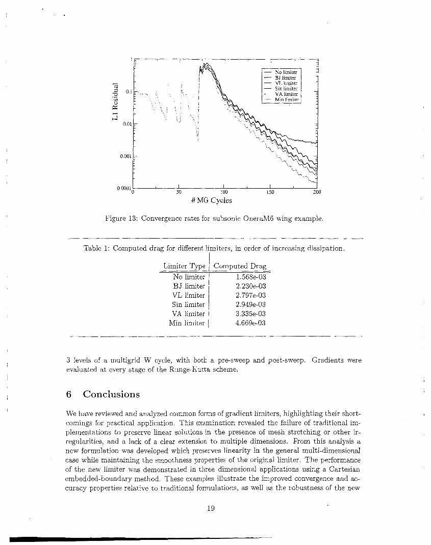
Figure 13 shows the same convergence histories using the new formulation with the five different limiters of figure 3 . The respective limiters are applied over the flow domain and at mesh interfaces using eq. (32). At cut cells next to the wing only the new van Leer formulation eq. (42) is used. Not surprisingly, the more dissipatiye the limiter the better the convergence. Barth- Jespersen, as before, has the most problems with convergence. Note however that this formulation is much improved over the version of figure 12, which is scalar at the cut cells and not linearity preserving at the mesh interfaces. I t makes a surprisingly large difference, even though those two categories of cells are only a small fraction of the mesh.

Although it is hard to say what the “exact” answer is, we expect the unlimited results to be the best on this mesh, and the answers to deteriorate with increasing dissipation. More evidence in this direction is seen by looking at the computed drag, which should converge to zero for this subsonic case. Table 1 gives the drag in order of increasing dissipation. All the iimiters shouid converge as the grid is refined, bur; for a given grid, tile less d i A p t i V e limiter gives the better drag count. This was computed on a rather coarse grid of 202K cells, to make the results more obvious.

The last example shows the performance of the new limiter on a problem with extremely complicated geometry and physics. The geometry is rather coarsely resolved, with only 1.8M cells in this calculation. The freestream Mach number is 18.5, with angle of attack 15 degrees. The density and pressure in the OMS pods and engine bells gets as low as The pressure on the orbiter’s nose is nearly 450 times that in the freestream, a range of nearly eight orders of magnitude. Exactly the same limiter settings with no ‘special tweaking are used for this case, despite the deep concavities, shown in figure 14(a). Figure 15 shows the convergence history of the residual and the forces for this case. This example used a

*

18

I I I I 1

50 100 I50 200

## MG Cycles

Figure 13: Convergence rates for subsonic OneraNIG wing example.

Limiter Type No limiter BJ limiter VL limiter Sin limiter VA limiter

Min limiter

Computed Drag 1.568e-03 2.230e-03 2.797e-63 2.949e-03 3.335e-03 4.669e-03

3 levels of a multigrid W cycle, with both a pre-sweep and post-sweep. Gradients were evaluated at every stage of the Runge-Kutta scheme.

6 Conclusions

We have reviewed and analyzed common forms of gradient limiters: highlighting their short- comings for practical application. This examination revealed the failure of traditional irn- plementations to preserve linear solutions in the presence of mesh stretching or other ir- regularities, and a lack of a clear extension t o multiple dimensions. From this analysis a new formulation was developed which preserves linearity in the general multi-dimensional case while maintainir,g the snoothness properties of the original limiter. The performame of the new limiter was demonstrated in three dimensional applications using a Cartesian embedded-boundary method. These examples illustrate the improved convergence and ac- curacy properties relative to traditional formulations, as well as the robustness of the new

19

Figure 14: Orbiter calculation using 1.8M cell mesh: Mach 18.5 at 15 degrees angle of attack. The contours show the log of pressure. The left figure also shows some streamlines of the flow in black. Both the complex geometry and complicated physics of the flow field are apparent.

- L1 Residual

o .3k - X ForcelMoment

! \ - Y ForcelMoment i '> - 2 ForcelMoment -

t 1 I I

0 100 200 -0.1 L

## MG Cycles

Figure 15: Convergence rate of L1 residual for orbiter calculation. Also shown are the computed forces at each iteration.

20

fUi 111.

While this work has focussed on linearity preserving limiters. a rich area for future work is limiting for higher order methods. This is especially true in multiple spatial dimensions where the savings from higher order schemes are particularly attractive.

7 Acknowledgements

We thank Jonathan Goodman for insightful discussions. Marsha Berger was supported by AFOSR grant F19620-00-0099 and by DOE grants DEFG02-00ER25053 and DEFC02- 0 lER25472.

References

[l] M. Aftosmis, M. Berger, and G. Adomavicius. A parallel multilevel method for a d a p tively refined Cartesian grids with embedded boundaries. AIAA-2000- 0808, January 2000.

[2] M. Aftosmis, D. Gaitonde, and T. Sean Tavares. On the accuracy, stability and mono- tonicity of various reconstruction algorithms for unstructured meshes. AIAA-94-0415, January 1994.

[3] Tim Earth. X Z E G ~ C ~ methods and error esti~iatitsii f i j i cofiseit-atiofi ~ W S 011 struc- tured and unstructured meshes. In Von K a m a n Institute Computational Fhid Dy- namics Lectures Notes, 2003.

[4] P. Coleiia and P. 'vTioodward. The piecewise parabolic method (PFM) for gas-dynamicai simulations. J. Comp. Phys., 54(1):174-201, 1984.

[5] J.B. Goodman and R.J. LeVeque. -4 geometric approach to high resolution TVD schemes. SIAM J. Num. Anal., 25, 1988.

[6] A. Harten. High resolution schemes for hyperbolic conservation laws. J. Comp. Phys., 49 : 35 7-393, 1 983.

[7] M.E. Hubbard. h/lultidimensional slope limiters for MUSCL-type finite volume schemes GE uixtiiictured grids. J. COZ~. P h p , 155:54-74, 1993.

[8] Carl Ollivier-Gooch. Quasi-EN0 schemes for unstructured meshes based on unlimited data-dependent least-squares reconstruction. J. Comp. Phys., 133:6-17, 1997.

[9] W. J. Rider and D. B. Kothe. Constrained minimization for monotonic reconstruction. AIAA-97-2G36, 1397.

[lo] Jeff Saltzman. Monotonic difference schemes for the linear advection equation in two and three dimensions. Technical Report 87-2479, Los Alamos National Laboratory, 1987.

[l I] S .P. Spekreijse. Multigrid discretization of monotone second-order discretizations of hyperbolic conservation laws. Math. Comp., 49, 1987.

21

[lzj P.K. Sweby. High resoiutiori schemes usirig fiux iiniiters for hvperboiic coiiservacion laws. SIAiW J. Num. Anal., 21, 1984.

[13] V. Venkatakrishnan. Convergence to steady state solutions of the Euler equations on unstructured grids with limiters. J. Comp. Phys., 118:120-130, 1995.

[14] S. T. Zalesak. Fully intiltidimensional fiux-corrected transport algorithms for fiuids. J . Comp. Phys., 31:335-362, 1979.

22

This work is an extended abstract tG be submitted to the 43nd Aerospace sciences meef- ing and exhibit session on applied CFD. The conference will be in Reno NV Jan 6-1 1, 2005. This paper examines the behavior of flux and slope limiters on non-uniform grids in multiple dimensions. We note that on non-uniform grids the standard scalar formulation in practical use today sacrifices k-exacctness even for linear solutions, impacting both accuracy and convergence. We rewrite some well-known limiters in a new way to high- light their underlying symmetry, and use this to examine both traditional and new lim-

shoiii results dennonstizting impioved acmracy and cocveigence using a combination of model problems and complex three-dimensional examples.

itci f ~ i i i ~ ~ i k i t i ~ i i ~ . 'A'c ~ C V ~ G I ; 2 GCZ &k~~.ti~ii.$ kiitci iii ~ d t i p l ~ C~~ZCX~GSS, 2 ~ 2