linearisation & lyapunov equation - university of … tutorial on eg4321/eg7040 nonlinear...
TRANSCRIPT

.
.
.
.
.
.
.
.
.
.
.
.
.
.
.
.
.
.
.
.
.
.
.
.
.
.
.
.
.
.
.
.
.
.
.
.
.
.
.
.
2nd Tutorial on EG4321/EG7040 Nonlinear ControlLinearisation & Lyapunov Equation
Dr. Angeliki Lekka1
1Control Systems Research GroupDepartment of Engineering, University of Leicester
March 2, 2017
Dr. Angeliki Lekka ([email protected]) Linearisation & Lyapunov March 2, 2017 1 / 22
.
.
.
.
.
.
.
.
.
.
.
.
.
.
.
.
.
.
.
.
.
.
.
.
.
.
.
.
.
.
.
.
.
.
.
.
.
.
.
.
Important things to remember
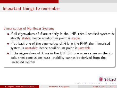
Linearisation of Nonlinear Systems
if all eigenvalues of A are strictly in the LHP, then linearised system isstrictly stable, hence equilibrium point is stable
if at least one of the eigenvalues of A is in the RHP, then linearisedsystem is unstable, hence equilibrium point is unstable
if the eigenvalues of A are in the LHP but one or more are on the jωaxis, then conclusions w.r.t. stability cannot be derived from thelinearised system
Dr. Angeliki Lekka ([email protected]) Linearisation & Lyapunov March 2, 2017 2 / 22

.
.
.
.
.
.
.
.
.
.
.
.
.
.
.
.
.
.
.
.
.
.
.
.
.
.
.
.
.
.
.
.
.
.
.
.
.
.
.
.
Important things to remember
From Lecture 4
If matrix A has negative eigenvalues, there exists a matrix P > 0 satisfyingthe Lyapunov equation A′P + PA = −Q
Steps to solve the Lyapunov equation
choose a positive definite matrix Q
Usually, Q = I is chosen (there is a reason for this)
solve for P from the Lyapunov equation
P should be square and symmetric (if it is not, we can turn it to one)
check whether P is positive definite
Definiteness defined only for square matrices
Dr. Angeliki Lekka ([email protected]) Linearisation & Lyapunov March 2, 2017 3 / 22
.
.
.
.
.
.
.
.
.
.
.
.
.
.
.
.
.
.
.
.
.
.
.
.
.
.
.
.
.
.
.
.
.
.
.
.
.
.
.
.
Exercise Sheet 3, Question 1 (1)
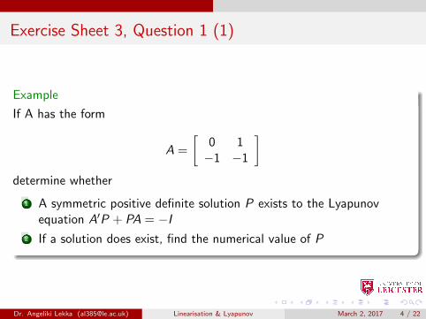
Example
If A has the form
A =
[0 1−1 −1
]determine whether
1 A symmetric positive definite solution P exists to the Lyapunovequation A′P + PA = −I
2 If a solution does exist, find the numerical value of P
Dr. Angeliki Lekka ([email protected]) Linearisation & Lyapunov March 2, 2017 4 / 22

.
.
.
.
.
.
.
.
.
.
.
.
.
.
.
.
.
.
.
.
.
.
.
.
.
.
.
.
.
.
.
.
.
.
.
.
.
.
.
.
Exercise Sheet 3, Question 1 (2)
To satisfy the 1st part, the eigenvalues of A must have negative real parts;we must solve the characteristic equation det(λI − A) = 0
det(λI − A) =
∣∣∣∣[ λ 00 λ
]−
[0 1−1 −1
]∣∣∣∣=
∣∣∣∣[ (λ− 0) (0− 1)(0− (−1)) (λ− (−1))
]∣∣∣∣=
∣∣∣∣[ λ −11 λ+ 1
]∣∣∣∣= λ(λ+ 1)− (1(−1)) = 0
= λ2 + λ+ 1 = 0 (1)
Dr. Angeliki Lekka ([email protected]) Linearisation & Lyapunov March 2, 2017 5 / 22
.
.
.
.
.
.
.
.
.
.
.
.
.
.
.
.
.
.
.
.
.
.
.
.
.
.
.
.
.
.
.
.
.
.
.
.
.
.
.
.
Exercise Sheet 3, Question 1 (3)
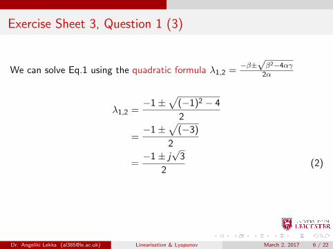
We can solve Eq.1 using the quadratic formula λ1,2 =−β±
√β2−4αγ2α
λ1,2 =−1±
√(−1)2 − 4
2
=−1±
√(−3)
2
=−1± j
√3
2(2)
Since the eigenvalues have negative real parts, a positive definite solutionto the Lyapunov equation does exist
Dr. Angeliki Lekka ([email protected]) Linearisation & Lyapunov March 2, 2017 6 / 22

.
.
.
.
.
.
.
.
.
.
.
.
.
.
.
.
.
.
.
.
.
.
.
.
.
.
.
.
.
.
.
.
.
.
.
.
.
.
.
.
Exercise Sheet 3, Question 1 (3)
We can solve Eq.1 using the quadratic formula λ1,2 =−β±
√β2−4αγ2α
λ1,2 =−1±
√(−1)2 − 4
2
=−1±
√(−3)
2
=−1± j
√3
2(2)
Since the eigenvalues have negative real parts, a positive definite solutionto the Lyapunov equation does exist
Dr. Angeliki Lekka ([email protected]) Linearisation & Lyapunov March 2, 2017 6 / 22
.
.
.
.
.
.
.
.
.
.
.
.
.
.
.
.
.
.
.
.
.
.
.
.
.
.
.
.
.
.
.
.
.
.
.
.
.
.
.
.
Exercise Sheet 3, Question 1 (4)
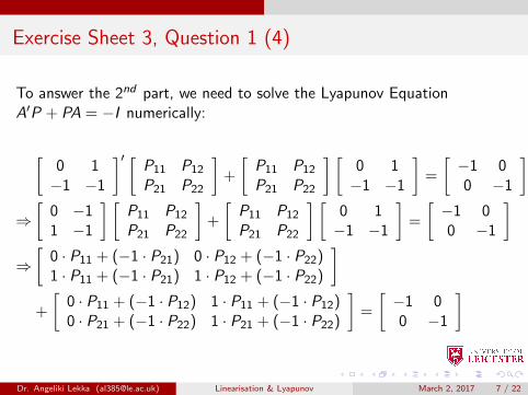
To answer the 2nd part, we need to solve the Lyapunov EquationA′P + PA = −I numerically:
[0 1−1 −1
]′ [P11 P12
P21 P22
]+
[P11 P12
P21 P22
] [0 1−1 −1
]=
[−1 00 −1
]⇒
[0 −11 −1
] [P11 P12
P21 P22
]+
[P11 P12
P21 P22
] [0 1−1 −1
]=
[−1 00 −1
]⇒
[0 · P11 + (−1 · P21) 0 · P12 + (−1 · P22)1 · P11 + (−1 · P21) 1 · P12 + (−1 · P22)
]+
[0 · P11 + (−1 · P12) 1 · P11 + (−1 · P12)0 · P21 + (−1 · P22) 1 · P21 + (−1 · P22)
]=
[−1 00 −1
]
Dr. Angeliki Lekka ([email protected]) Linearisation & Lyapunov March 2, 2017 7 / 22

.
.
.
.
.
.
.
.
.
.
.
.
.
.
.
.
.
.
.
.
.
.
.
.
.
.
.
.
.
.
.
.
.
.
.
.
.
.
.
.
Exercise Sheet 3, Question 1 (5)
⇒[
−P21 −P22
P11 − P21 P12 − P22)
]+
[−P12 P11 − P12
−P22 P21 − P22
]=
[−1 00 −1
]⇒
[−P21 − P12 P11 − P12 − P22
P11 − P21 − P22 −2P22 + P12 + P21
]=
[−1 00 −1
]Since P is chosen symmetric, i.e. P12 = P21, we get:
⇒[
−2P12 P11 − P12 − P22
P11 − P12 − P22 −2P22 + 2P12
]=
[−1 00 −1
]
Dr. Angeliki Lekka ([email protected]) Linearisation & Lyapunov March 2, 2017 8 / 22
.
.
.
.
.
.
.
.
.
.
.
.
.
.
.
.
.
.
.
.
.
.
.
.
.
.
.
.
.
.
.
.
.
.
.
.
.
.
.
.
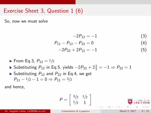
Exercise Sheet 3, Question 1 (6)
So, now we must solve
−2P12 = −1 (3)
P11 − P12 − P22 = 0 (4)
−2P22 + 2P12 = −1 (5)
From Eq.3, P12 = 1/2
Substituting P12 in Eq.5, yields −2P22 + 212 = −1 ⇒ P22 = 1
Substituting P12 and P22 in Eq.4, we getP11 − 1/2 − 1 = 0 ⇒ P11 = 3/2
and hence,
P =
[3/2 1/21/2 1
]Dr. Angeliki Lekka ([email protected]) Linearisation & Lyapunov March 2, 2017 9 / 22
.
.
.
.
.
.
.
.
.
.
.
.
.
.
.
.
.
.
.
.
.
.
.
.
.
.
.
.
.
.
.
.
.
.
.
.
.
.
.
.
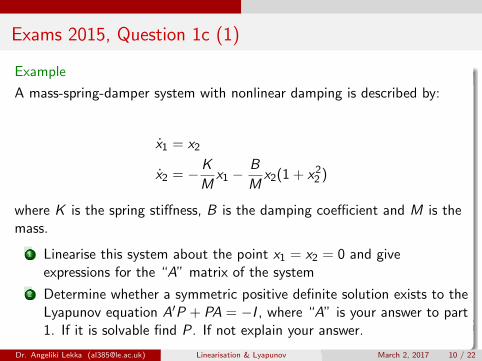
Exams 2015, Question 1c (1)
Example
A mass-spring-damper system with nonlinear damping is described by:
x1 = x2
x2 = −K
Mx1 −
B
Mx2(1 + x22 )
where K is the spring stiffness, B is the damping coefficient and M is themass.
1 Linearise this system about the point x1 = x2 = 0 and giveexpressions for the “A” matrix of the system
2 Determine whether a symmetric positive definite solution exists to theLyapunov equation A′P + PA = −I , where “A” is your answer to part1. If it is solvable find P. If not explain your answer.
Dr. Angeliki Lekka ([email protected]) Linearisation & Lyapunov March 2, 2017 10 / 22

.
.
.
.
.
.
.
.
.
.
.
.
.
.
.
.
.
.
.
.
.
.
.
.
.
.
.
.
.
.
.
.
.
.
.
.
.
.
.
.
Exams 2015, Question 1c (2)
To linearise the nonlinear mass-spring-damper system we must calculatethe Jacobian matrix A:
A =∂f
∂x
∣∣∣∣x1=x2=0
=
[∂f1∂x1
∂f1∂x2
∂f2∂x1
∂f2∂x2
]∣∣∣∣∣x1=x2=0
=
[0 1
− KM − B
M − 3BM x22
]∣∣∣∣x1=x2=0
Evaluating the Jacobian matrix at x1 = x2 = 0, yields:
A =
[0 1
− KM − B
M
]
Dr. Angeliki Lekka ([email protected]) Linearisation & Lyapunov March 2, 2017 11 / 22
.
.
.
.
.
.
.
.
.
.
.
.
.
.
.
.
.
.
.
.
.
.
.
.
.
.
.
.
.
.
.
.
.
.
.
.
.
.
.
.
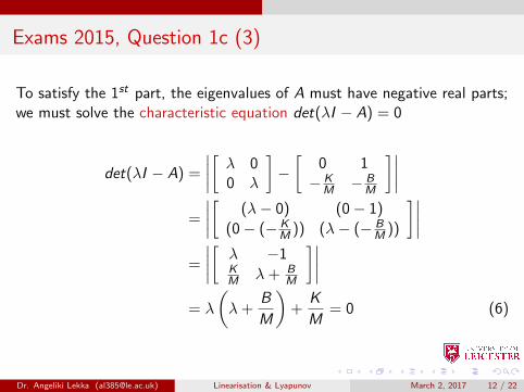
Exams 2015, Question 1c (3)
To satisfy the 1st part, the eigenvalues of A must have negative real parts;we must solve the characteristic equation det(λI − A) = 0
det(λI − A) =
∣∣∣∣[ λ 00 λ
]−[
0 1
− KM − B
M
]∣∣∣∣=
∣∣∣∣[ (λ− 0) (0− 1)
(0− (− KM )) (λ− (− B
M ))
]∣∣∣∣=
∣∣∣∣[ λ −1KM λ+ B
M
]∣∣∣∣= λ
(λ+
B
M
)+
K
M= 0 (6)
Dr. Angeliki Lekka ([email protected]) Linearisation & Lyapunov March 2, 2017 12 / 22
.
.
.
.
.
.
.
.
.
.
.
.
.
.
.
.
.
.
.
.
.
.
.
.
.
.
.
.
.
.
.
.
.
.
.
.
.
.
.
.
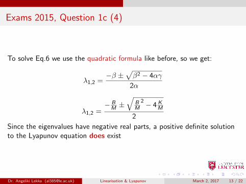
Exams 2015, Question 1c (4)
To solve Eq.6 we use the quadratic formula like before, so we get:
λ1,2 =−β ±
√β2 − 4αγ
2α
λ1,2 =− B
M ±√
BM
2 − 4 KM
2
Since the eigenvalues have negative real parts, a positive definite solutionto the Lyapunov equation does exist
Dr. Angeliki Lekka ([email protected]) Linearisation & Lyapunov March 2, 2017 13 / 22

.
.
.
.
.
.
.
.
.
.
.
.
.
.
.
.
.
.
.
.
.
.
.
.
.
.
.
.
.
.
.
.
.
.
.
.
.
.
.
.
Exams 2015, Question 1c (5)
To answer the 2nd part, we need to solve the Lyapunov EquationA′P + PA = −I numerically:[
0 1
− KM − B
M
]′ [P11 P12
P21 P22
]+
[P11 P12
P21 P22
] [0 1
− KM − B
M
]=
[−1 00 −1
]⇒
[0 − K
M
1 − BM
] [P11 P12
P21 P22
]+
[P11 P12
P21 P22
] [0 1
− KM − B
M
]=
[−1 00 −1
]⇒
[0 · P11 + (− K
MP21) 0 · P12 + (− KMP22)
1 · P11 + (− BMP21) 1 · P12 + (− B
MP22)
]+
[0 · P11 + (− K
MP12) 1 · P11 + (− BMP12)
0 · P21 + (− KMP22) 1 · P21 + (− B
MP22)
]=
[−1 00 −1
]
Dr. Angeliki Lekka ([email protected]) Linearisation & Lyapunov March 2, 2017 14 / 22
.
.
.
.
.
.
.
.
.
.
.
.
.
.
.
.
.
.
.
.
.
.
.
.
.
.
.
.
.
.
.
.
.
.
.
.
.
.
.
.
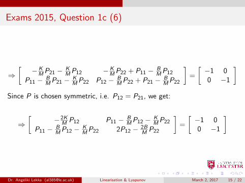
Exams 2015, Question 1c (6)
⇒[
− KMP21 − K
MP12 − KMP22 + P11 − B
MP12
P11 − BMP21 − K
MP22 P12 − BMP22 + P21 − B
MP22
]=
[−1 00 −1
]Since P is chosen symmetric, i.e. P12 = P21, we get:
⇒[
−2KM P12 P11 − B
MP12 − KMP22
P11 − BMP12 − K
MP22 2P12 − 2BM P22
]=
[−1 00 −1
]
Dr. Angeliki Lekka ([email protected]) Linearisation & Lyapunov March 2, 2017 15 / 22

.
.
.
.
.
.
.
.
.
.
.
.
.
.
.
.
.
.
.
.
.
.
.
.
.
.
.
.
.
.
.
.
.
.
.
.
.
.
.
.
Exams 2015, Question 1c (7)
So, now we must solve
−2K
MP12 = −1 (7)
P11 −B
MP12 −
K
MP22 = 0 (8)
2P12 −2B
MP22 = −1 (9)
From Eq.7, P12 =12MK
Substituting P12 in Eq.9, yields
21
2
M
K− 2B
MP22 = −1 ⇒ −2B
MP22 = −1− M
K
⇒ P22 =
(1 +
M
K
)M
2B⇒ P22 =
1
2
M
B
(K +M
K
)Dr. Angeliki Lekka ([email protected]) Linearisation & Lyapunov March 2, 2017 16 / 22
.
.
.
.
.
.
.
.
.
.
.
.
.
.
.
.
.
.
.
.
.
.
.
.
.
.
.
.
.
.
.
.
.
.
.
.
.
.
.
.
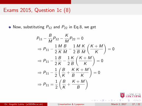
Exams 2015, Question 1c (8)
Now, substituting P12 and P22 in Eq.8, we get
P11 −B
MP12 −
K
MP22 = 0
⇒ P11 −1
2
M
K
B
M− 1
2
M
B
K
M
(K +M
K
)= 0
⇒ P11 −1
2
B
K− 1
2
K
B
(K +M
K
)= 0
⇒ P11 −1
2
(B
K+
K
B
K +M
K
)= 0
⇒ P11 =1
2
(B
K+
K +M
B
)
Dr. Angeliki Lekka ([email protected]) Linearisation & Lyapunov March 2, 2017 17 / 22
.
.
.
.
.
.
.
.
.
.
.
.
.
.
.
.
.
.
.
.
.
.
.
.
.
.
.
.
.
.
.
.
.
.
.
.
.
.
.
.
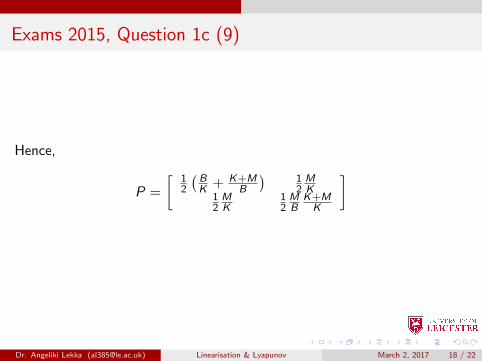
Exams 2015, Question 1c (9)
Hence,
P =
[12
(BK + K+M
B
)12MK
12MK
12MB
K+MK
]
Dr. Angeliki Lekka ([email protected]) Linearisation & Lyapunov March 2, 2017 18 / 22
.
.
.
.
.
.
.
.
.
.
.
.
.
.
.
.
.
.
.
.
.
.
.
.
.
.
.
.
.
.
.
.
.
.
.
.
.
.
.
.
Suggestions for personal study/revision
Be familiar with stability concepts w.r.t the eigenvalues of a matrix
Revise on derivatives and partial derivatives, so you are able tocompute Jacobian matrices (perform linearisation)
Be familiar with the concepts of positiveness & negativeness ofmatrices (ability to solve the Lyapunov equation)
Be familiar with the chain rule - particularly useful throughout thecourse
Dr. Angeliki Lekka ([email protected]) Linearisation & Lyapunov March 2, 2017 19 / 22
.
.
.
.
.
.
.
.
.
.
.
.
.
.
.
.
.
.
.
.
.
.
.
.
.
.
.
.
.
.
.
.
.
.
.
.
.
.
.
.
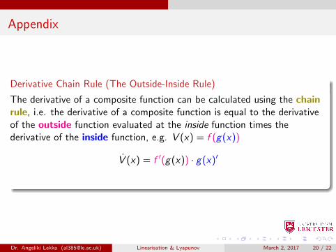
Appendix
Derivative Chain Rule (The Outside-Inside Rule)
The derivative of a composite function can be calculated using the chainrule, i.e. the derivative of a composite function is equal to the derivativeof the outside function evaluated at the inside function times thederivative of the inside function, e.g. V (x) = f (g(x))
V (x) = f ′(g(x)) · g(x)′
Dr. Angeliki Lekka ([email protected]) Linearisation & Lyapunov March 2, 2017 20 / 22
.
.
.
.
.
.
.
.
.
.
.
.
.
.
.
.
.
.
.
.
.
.
.
.
.
.
.
.
.
.
.
.
.
.
.
.
.
.
.
.
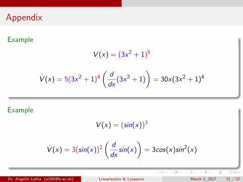
Appendix
Example
V (x) = (3x2 + 1)5
V (x) = 5(3x2 + 1)4(
d
dx(3x2 + 1)
)= 30x(3x2 + 1)4
Example
V (x) = (sin(x))3
V (x) = 3(sin(x))2(
d
dxsin(x)
)= 3cos(x)sin2(x)
Dr. Angeliki Lekka ([email protected]) Linearisation & Lyapunov March 2, 2017 21 / 22