linear variable differential transformer design and verification

4

Linear Variable Differential Transformer Design and Verification Using MATLAB and

Finite Element Analysis

Lutfi Al-Sharif, Mohammad Kilani, Sinan Taifour, Abdullah Jamal Issa, Eyas Al-Qaisi, Fadi Awni Eleiwi and Omar Nabil Kamal

Mechatronics Engineering Department, University of Jordan Jordan

1. Introduction

The linear variable differential transformer is one of the most widely used transducers for measuring linear displacement. It offers many advantages over potentio-metric linear transducers such as frictionless measurement, infinite mechanical life, excellent resolution and good repeatability (Herceg, 1972). Its main disadvantages are its dynamic response and the effects of the exciting frequency. General guidelines regarding the selection of an LVDT for a certain application can be found in (Herceg, 2006). The LVDT is also used as a secondary transducer in various measurement systems. A primary transducer is used to convert the measurand into a displacement. The LVDT is then used to measure that displacement. Examples are: 1. Pressure measurement whereby the displacement of a diaphragm or Bourdon tube is

detected by the LVDT (e.g., diaphragm type pressure transducer, (Daly et al., 1984)). 2. Acceleration measurement whereby the displacement of a mass is measured by the

LVDT (e.g., LVDT used within an accelerometer, (Morris, 2001). 3. Force measurement whereby the displacement of an elastic element subjected to the

force is measured by the LVDT (e.g., ring type load cell, (Daly et al., 1984)). The classical method of LVDT analysis and design is based on the use of approximate equations as shown in (Herceg, 1972) and (Popovic et al., 1999). These equations suffer from inaccuracy especially from end effects. More novel methods for design employ finite element methods (Syulski et al., 1992), artificial neural networks (Mishra et al., 2006) and (Mishra et al., 2005). The dynamic response of the LVDT is discussed in (Doebelin, 2003). The LVDT has also been integrated into linear actuators (Wu et al., 2008).

2. General overview

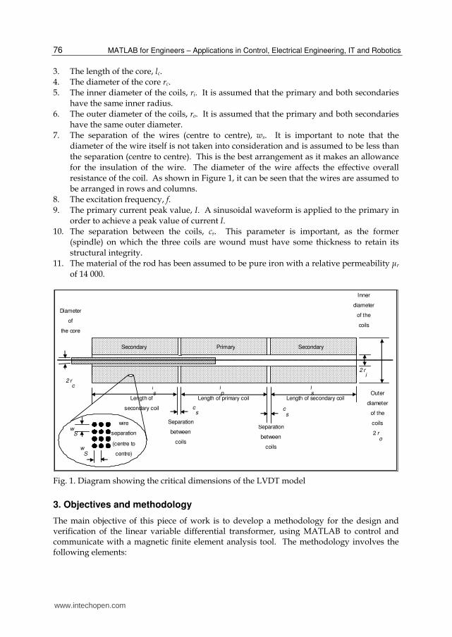
A diagram showing the dimensional parameters of the LVDT is shown in Figure 1 below. The important parameters that are taken into consideration in the design of the LVDT are listed below. 1. The length of the primary coil, lp. 2. The length of the secondary coil, ls. It is assumed that both secondaries have the same

length.

www.intechopen.com

MATLAB for Engineers – Applications in Control, Electrical Engineering, IT and Robotics 76

3. The length of the core, lc. 4. The diameter of the core rc.

5. The inner diameter of the coils, ri. It is assumed that the primary and both secondaries have the same inner radius.

6. The outer diameter of the coils, ro. It is assumed that the primary and both secondaries have the same outer diameter.

7. The separation of the wires (centre to centre), ws. It is important to note that the

diameter of the wire itself is not taken into consideration and is assumed to be less than

the separation (centre to centre). This is the best arrangement as it makes an allowance

for the insulation of the wire. The diameter of the wire affects the effective overall

resistance of the coil. As shown in Figure 1, it can be seen that the wires are assumed to

be arranged in rows and columns.

8. The excitation frequency, f.

9. The primary current peak value, I. A sinusoidal waveform is applied to the primary in order to achieve a peak value of current I.

10. The separation between the coils, cs. This parameter is important, as the former (spindle) on which the three coils are wound must have some thickness to retain its

structural integrity. 11. The material of the rod has been assumed to be pure iron with a relative permeability μr

of 14 000.

Length of

secondary coil

Length of secondary coilLength of primary coil

SecondarySecondary Primary

wire

separation

(centre to

centre) w

S

2 ri

lp

ls

ls Outer

diameter

of the

coils

2 ro

cs

2 rc

Separation

between

coils

Separation

between

coils

cs

wS

Inner

diameter

of the

coils

Diameter

of

the core

Fig. 1. Diagram showing the critical dimensions of the LVDT model

3. Objectives and methodology

The main objective of this piece of work is to develop a methodology for the design and verification of the linear variable differential transformer, using MATLAB to control and communicate with a magnetic finite element analysis tool. The methodology involves the following elements:

www.intechopen.com

Linear Variable Differential Transformer Design and Verification Using MATLAB and Finite Element Analysis 77

1. The capturing and coding of a number of rules of thumb that are used to find initial

suitable values for the primary, secondaries and core length in relationship to the

required stroke. These rules of thumb have been based on industrial experience.

2. The use of a finite element model (finite element magnetic tool) that is used to find the

total flux linkage between the primary and the two secondaries based on a certain

position of the core.

3. The use of MATLAB as a control tool to call the finite element modeling tool in order to

find the output voltage of the two seconardies at each core position. MATLAB is then

used to repeat this process until the full curve is produced.

4. A MATLAB based graphical user interface (GUI) has also been developed to act as a

user friendly platform allowing the user to enter the required specification and to

derive the output voltage characteristics.

5. Theoretical verification has been carried out, whereby the equation for the total flux

linkage between two loops has been developed and then checked against the output of

the finite element model to ensure that it is producing correct results.

6. In order to provide practical verification, an LVDT has then been built and the output

measured and compared with the theoretical finite element outputs.

4. FEMM based model

The aim of the modeling methodology is to derive the transfer characteristic of an LVDT

with certain dimensions and parameters. The transfer characteristic (or output

characteristic) is a relationship between the displacement of the core and the output

resultant dc voltage. It is assumed that the two ac signals from the two secondaries are

processed by full wave rectifying them, smoothing the signals and then subtracting them.

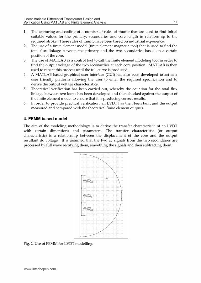
Fig. 2. Use of FEMM for LVDT modelling.

www.intechopen.com


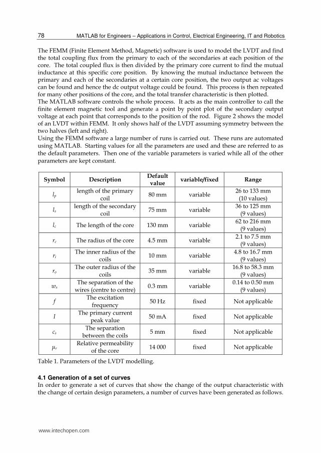
The FEMM (Finite Element Method, Magnetic) software is used to model the LVDT and find the total coupling flux from the primary to each of the secondaries at each position of the core. The total coupled flux is then divided by the primary core current to find the mutual inductance at this specific core position. By knowing the mutual inductance between the primary and each of the secondaries at a certain core position, the two output ac voltages can be found and hence the dc output voltage could be found. This process is then repeated for many other positions of the core, and the total transfer characteristic is then plotted. The MATLAB software controls the whole process. It acts as the main controller to call the finite element magnetic tool and generate a point by point plot of the secondary output voltage at each point that corresponds to the position of the rod. Figure 2 shows the model of an LVDT within FEMM. It only shows half of the LVDT assuming symmetry between the two halves (left and right). Using the FEMM software a large number of runs is carried out. These runs are automated using MATLAB. Starting values for all the parameters are used and these are referred to as the default parameters. Then one of the variable parameters is varied while all of the other parameters are kept constant.

Symbol Description Default value

variable/fixed Range

lp length of the primary

coil 80 mm variable

26 to 133 mm (10 values)

ls length of the secondary

coil 75 mm variable

36 to 125 mm (9 values)

lc The length of the core 130 mm variable 62 to 216 mm

(9 values)

rc The radius of the core 4.5 mm variable 2.1 to 7.5 mm

(9 values)

ri The inner radius of the

coils 10 mm variable

4.8 to 16.7 mm (9 values)

ro The outer radius of the

coils 35 mm variable

16.8 to 58.3 mm (9 values)

ws The separation of the

wires (centre to centre) 0.3 mm variable

0.14 to 0.50 mm (9 values)

f The excitation

frequency 50 Hz fixed Not applicable

I The primary current

peak value 50 mA fixed Not applicable

cs The separation

between the coils 5 mm fixed Not applicable

μr Relative permeability

of the core 14 000 fixed Not applicable

Table 1. Parameters of the LVDT modelling.

4.1 Generation of a set of curves In order to generate a set of curves that show the change of the output characteristic with the change of certain design parameters, a number of curves have been generated as follows.

www.intechopen.com


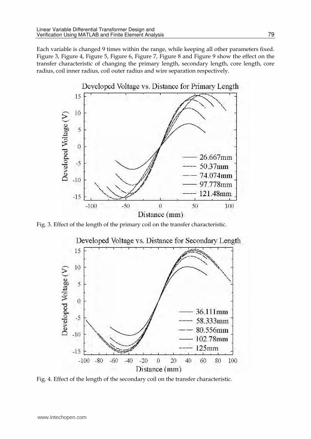
Each variable is changed 9 times within the range, while keeping all other parameters fixed. Figure 3, Figure 4, Figure 5, Figure 6, Figure 7, Figure 8 and Figure 9 show the effect on the transfer characteristic of changing the primary length, secondary length, core length, core radius, coil inner radius, coil outer radius and wire separation respectively.

Fig. 3. Effect of the length of the primary coil on the transfer characteristic.

Fig. 4. Effect of the length of the secondary coil on the transfer characteristic.

www.intechopen.com


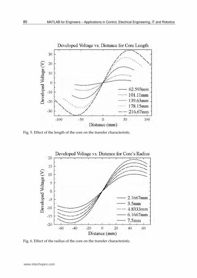
Fig. 5. Effect of the length of the core on the transfer characteristic.

Fig. 6. Effect of the radius of the core on the transfer characteristic.

www.intechopen.com


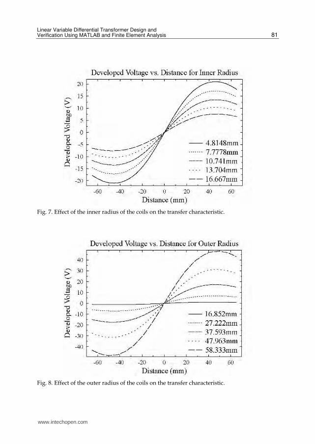
Fig. 7. Effect of the inner radius of the coils on the transfer characteristic.

Fig. 8. Effect of the outer radius of the coils on the transfer characteristic.

www.intechopen.com


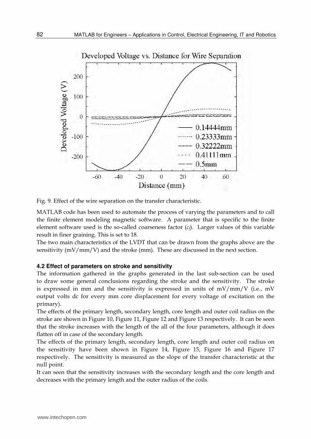
Fig. 9. Effect of the wire separation on the transfer characteristic.

MATLAB code has been used to automate the process of varying the parameters and to call

the finite element modeling magnetic software. A parameter that is specific to the finite

element software used is the so-called coarseness factor (cf). Larger values of this variable

result in finer graining. This is set to 18.

The two main characteristics of the LVDT that can be drawn from the graphs above are the

sensitivity (mV/mm/V) and the stroke (mm). These are discussed in the next section.

4.2 Effect of parameters on stroke and sensitivity

The information gathered in the graphs generated in the last sub-section can be used

to draw some general conclusions regarding the stroke and the sensitivity. The stroke

is expressed in mm and the sensitivity is expressed in units of mV/mm/V (i.e., mV

output volts dc for every mm core displacement for every voltage of excitation on the

primary).

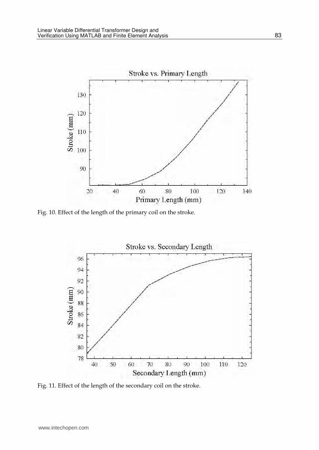
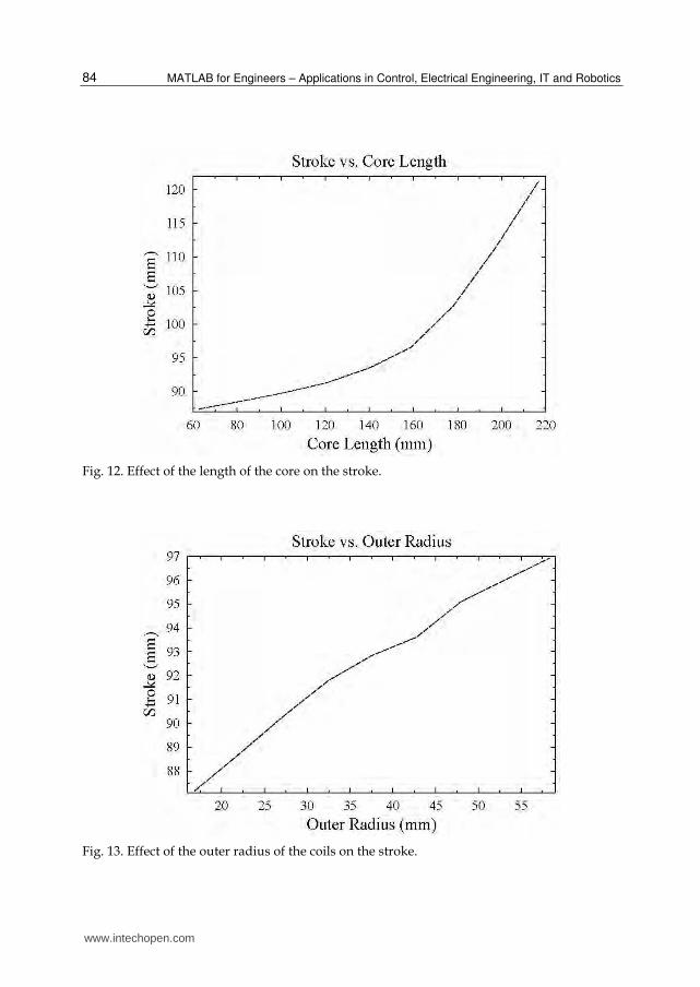
The effects of the primary length, secondary length, core length and outer coil radius on the

stroke are shown in Figure 10, Figure 11, Figure 12 and Figure 13 respectively. It can be seen

that the stroke increases with the length of the all of the four parameters, although it does

flatten off in case of the secondary length.

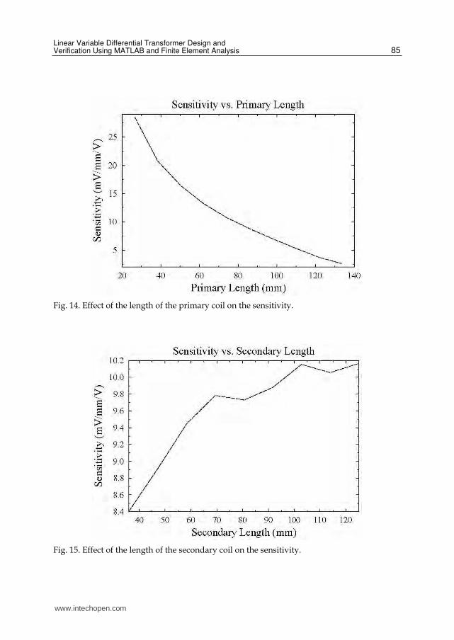
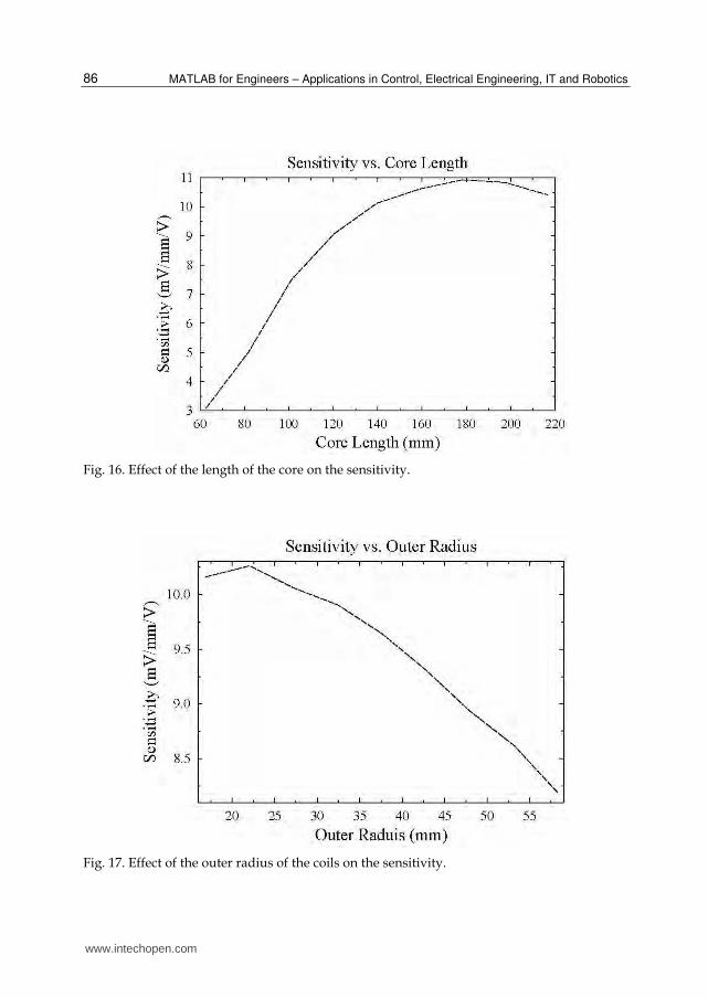
The effects of the primary length, secondary length, core length and outer coil radius on

the sensitivity have been shown in Figure 14, Figure 15, Figure 16 and Figure 17

respectively. The sensitivity is measured as the slope of the transfer characteristic at the

null point.

It can seen that the sensitivity increases with the secondary length and the core length and

decreases with the primary length and the outer radius of the coils.

www.intechopen.com


Fig. 10. Effect of the length of the primary coil on the stroke.

Fig. 11. Effect of the length of the secondary coil on the stroke.

www.intechopen.com


Fig. 12. Effect of the length of the core on the stroke.

Fig. 13. Effect of the outer radius of the coils on the stroke.

www.intechopen.com


Fig. 14. Effect of the length of the primary coil on the sensitivity.

Fig. 15. Effect of the length of the secondary coil on the sensitivity.

www.intechopen.com


Fig. 16. Effect of the length of the core on the sensitivity.

Fig. 17. Effect of the outer radius of the coils on the sensitivity.

www.intechopen.com


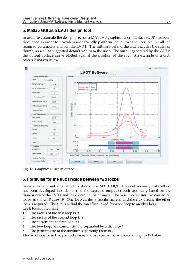
5. Matlab GUI as a LVDT design tool

In order to automate the design process, a MATLAB graphical user interface (GUI) has been developed in order to provide a user friendly platform that allows the user to enter all the required parameters and run the LVDT. The software behind the GUI includes the rules of thumb, as well as suggested default values to the user. The output generated by the GUI is the output voltage curve plotted against the position of the rod. An example of a GUI screen is shown below.

Fig. 18. Graphical User Interface.

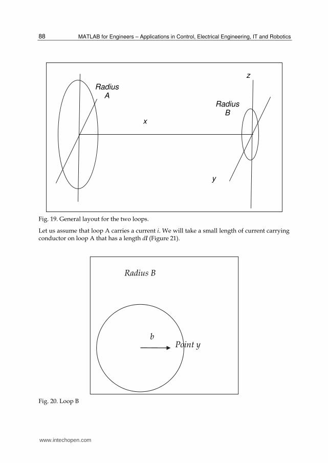
6. Formulae for the flux linkage between two loops

In order to carry out a partial verification of the MATLAB/FEA model, an analytical method has been developed in order to find the expected output of each secondary based on the dimensions of the LVDT and the current in the primary. The basic model uses two concentric loops as shown Figure 19. One loop carries a certain current, and the flux linking the other loop is required. The aim is to find the total flux linked from one loop to another loop. Let it be assumed that: 1. The radius of the first loop is A 2. The radius of the second loop is B 3. The current in the first loop is i 4. The two loops are concentric and separated by a distance h 5. The permittivity of the medium separating them is μ The two loops lie in two parallel planes and are concentric as shown in Figure 19 below.

www.intechopen.com


Fig. 19. General layout for the two loops.

Let us assume that loop A carries a current i. We will take a small length of current carrying conductor on loop A that has a length dl (Figure 21).

Fig. 20. Loop B

y

z

x

Radius B

Radius A

Radius B

Point y b

www.intechopen.com


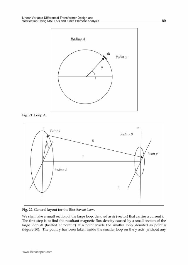
Fig. 21. Loop A.

Fig. 22. General layout for the Biot-Savart Law.

We shall take a small section of the large loop, denoted as dl (vector) that carries a current i. The first step is to find the resultant magnetic flux density caused by a small section of the large loop dl (located at point x) at a point inside the smaller loop, denoted as point y (Figure 20). The point y has been taken inside the smaller loop on the y axis (without any

Radius A

Point x

θ

dl

www.intechopen.com


loss of generality) at a distance b from the centre of the loop. The vector connecting points x and y represents the direction of the resultant magnetic flux density (Figure 22). We shall denote the vector that connects points x to y as R. Using Biot-savart law gives:

34

i dl RdB

R

µ ⋅ ⋅ ×=

⋅ π ⋅

(1)

The coordinates of point x are:

( )0, cos , sinA A⋅ θ ⋅ θ (2)

The coordinates of point y are:

( ), ,0h b (3)

The magnitude of R can be calculated as follows:

( ) ( )2 22 cos sinR h A b A= + ⋅ θ − + ⋅ θ (4)

2 2 2 2 2 2

2 2 2

cos 2 cos sin

2 cos

R h A bA b A

h A b bA

= + ⋅ θ − ⋅ θ + + ⋅ θ

= + + − ⋅ θ

(5)

This gives us the magnitude of R. We next find the components of the two vectors, R and dl:

[ ]cos sinR h b A A= − ⋅ θ − ⋅ θ

(6)

[ ]0 sin cosdl A d A d= − ⋅ θ ⋅ θ ⋅ θ ⋅ θ

(7)

We now turn to find the cross product of these two elements (note that we will only evaluate the x component as this is the component that is of interest to us).

( )

( )

2

32 2 2 2

cos

4 2 cos

i

i d A A b idB

h A b A b

µ ⋅ ⋅ θ ⋅ − ⋅ ⋅ θ=

⋅ π ⋅ + + − ⋅ ⋅ ⋅ θ

(8)

We have taken the x direction only as this is the direction that is perpendicular to the area of the smaller loop. This effect is only caused by a small strip dl of the larger loop. In order to find the effect of the whole larger loop on the point y, we need to integrate around the larger loop. This is done as follows:

( )

( )

22

32 2 20 2

cos

4 2 cos

iloop

i A A bdB d i

h A b A b

π µ ⋅ ⋅ − ⋅ ⋅ θ= θ

⋅ π ⋅ + + − ⋅ ⋅ ⋅ θ

(9)

If we now take an annulus of radius b inside the smaller loop, we can see that by symmetry, the value of the magnetic flux density component that is perpendicular to the area of the

www.intechopen.com


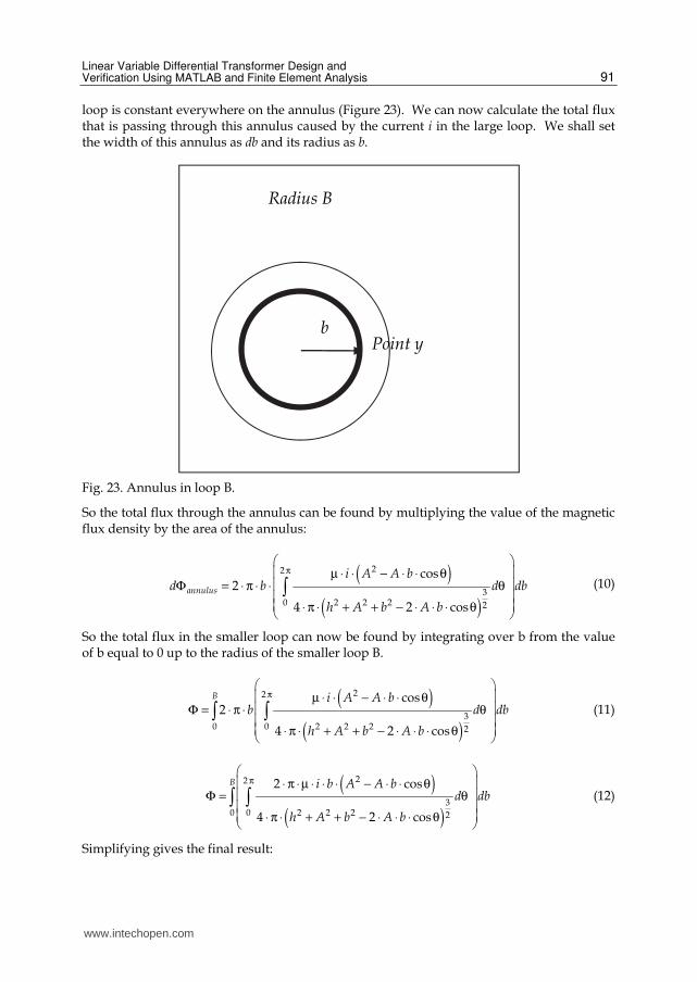
loop is constant everywhere on the annulus (Figure 23). We can now calculate the total flux that is passing through this annulus caused by the current i in the large loop. We shall set the width of this annulus as db and its radius as b.

Fig. 23. Annulus in loop B.

So the total flux through the annulus can be found by multiplying the value of the magnetic flux density by the area of the annulus:

( )

( )

22

32 2 20 2

cos2

4 2 cos

annulus

i A A bd b d db

h A b A b

π µ ⋅ ⋅ − ⋅ ⋅ θ Φ = ⋅ π ⋅ ⋅ θ ⋅ π ⋅ + + − ⋅ ⋅ ⋅ θ (10)

So the total flux in the smaller loop can now be found by integrating over b from the value of b equal to 0 up to the radius of the smaller loop B.

( )

( )

22

32 2 20 0 2

cos2

4 2 cos

B i A A bb d db

h A b A b

π µ ⋅ ⋅ − ⋅ ⋅ θ Φ = ⋅ π ⋅ θ ⋅ π ⋅ + + − ⋅ ⋅ ⋅ θ

(11)

( )

( )

22

32 2 20 0 2

2 cos

4 2 cos

B i b A A bd db

h A b A b

π ⋅ π ⋅ µ ⋅ ⋅ ⋅ − ⋅ ⋅ θ Φ = θ ⋅ π ⋅ + + − ⋅ ⋅ ⋅ θ (12)

Simplifying gives the final result:

Radius B

Point y b

www.intechopen.com


( )

( )

22

32 2 20 0 2

cos

2 2 cos

B i b A A bd db

h A b A b

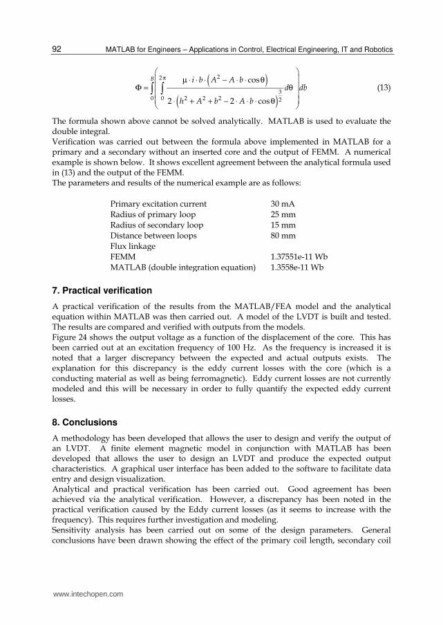
π µ ⋅ ⋅ ⋅ − ⋅ ⋅ θ Φ = θ ⋅ + + − ⋅ ⋅ ⋅ θ (13)

The formula shown above cannot be solved analytically. MATLAB is used to evaluate the double integral. Verification was carried out between the formula above implemented in MATLAB for a primary and a secondary without an inserted core and the output of FEMM. A numerical example is shown below. It shows excellent agreement between the analytical formula used in (13) and the output of the FEMM. The parameters and results of the numerical example are as follows:

Primary excitation current 30 mA

Radius of primary loop 25 mm

Radius of secondary loop 15 mm

Distance between loops 80 mm

Flux linkage

FEMM 1.37551e-11 Wb

MATLAB (double integration equation) 1.3558e-11 Wb

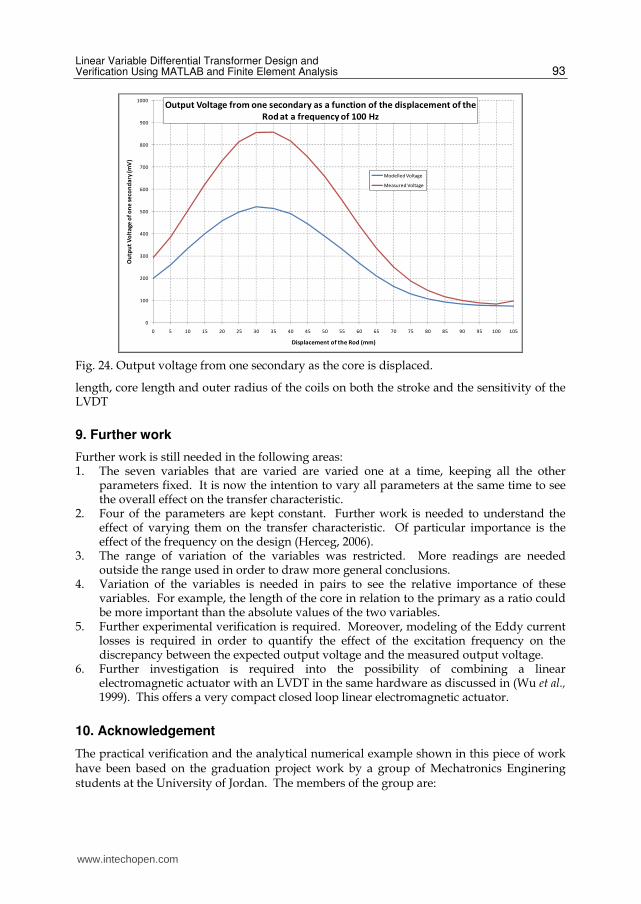
7. Practical verification

A practical verification of the results from the MATLAB/FEA model and the analytical equation within MATLAB was then carried out. A model of the LVDT is built and tested. The results are compared and verified with outputs from the models. Figure 24 shows the output voltage as a function of the displacement of the core. This has been carried out at an excitation frequency of 100 Hz. As the frequency is increased it is noted that a larger discrepancy between the expected and actual outputs exists. The explanation for this discrepancy is the eddy current losses with the core (which is a conducting material as well as being ferromagnetic). Eddy current losses are not currently modeled and this will be necessary in order to fully quantify the expected eddy current losses.

8. Conclusions

A methodology has been developed that allows the user to design and verify the output of an LVDT. A finite element magnetic model in conjunction with MATLAB has been developed that allows the user to design an LVDT and produce the expected output characteristics. A graphical user interface has been added to the software to facilitate data entry and design visualization. Analytical and practical verification has been carried out. Good agreement has been achieved via the analytical verification. However, a discrepancy has been noted in the practical verification caused by the Eddy current losses (as it seems to increase with the frequency). This requires further investigation and modeling. Sensitivity analysis has been carried out on some of the design parameters. General conclusions have been drawn showing the effect of the primary coil length, secondary coil

www.intechopen.com


Fig. 24. Output voltage from one secondary as the core is displaced.

length, core length and outer radius of the coils on both the stroke and the sensitivity of the LVDT

9. Further work

Further work is still needed in the following areas: 1. The seven variables that are varied are varied one at a time, keeping all the other

parameters fixed. It is now the intention to vary all parameters at the same time to see the overall effect on the transfer characteristic.

2. Four of the parameters are kept constant. Further work is needed to understand the effect of varying them on the transfer characteristic. Of particular importance is the effect of the frequency on the design (Herceg, 2006).

3. The range of variation of the variables was restricted. More readings are needed outside the range used in order to draw more general conclusions.

4. Variation of the variables is needed in pairs to see the relative importance of these variables. For example, the length of the core in relation to the primary as a ratio could be more important than the absolute values of the two variables.

5. Further experimental verification is required. Moreover, modeling of the Eddy current losses is required in order to quantify the effect of the excitation frequency on the discrepancy between the expected output voltage and the measured output voltage.

6. Further investigation is required into the possibility of combining a linear electromagnetic actuator with an LVDT in the same hardware as discussed in (Wu et al., 1999). This offers a very compact closed loop linear electromagnetic actuator.

10. Acknowledgement

The practical verification and the analytical numerical example shown in this piece of work have been based on the graduation project work by a group of Mechatronics Enginering students at the University of Jordan. The members of the group are:

0

100

200

300

400

500

600

700

800

900

1000

0 5 10 15 20 25 30 35 40 45 50 55 60 65 70 75 80 85 90 95 100 105

Ou

tpu

t V

olt

age

of

on

e s

eco

nd

ary

(m

V)

Displacement of the Rod (mm)

Output Voltage from one secondary as a function of the displacement of the

Rod at a frequency of 100 Hz

Modelled Voltage

Measured Voltage

www.intechopen.com


• “Mohammad Hussam ALDein" Omar Ali Bolad

• Anas Imad Ahmad Farouqa

• Anas Abdullah Ahmad Al-shoubaki

• Baha' Abd-Elrazzaq Ahmad Alsuradi

• Yazan Khalid Talib Al-diqs

11. References

Beckwith, Buck & Marangoni, (1982), Mechanical Measurements, Third Edition, 1982. Daly, James; Riley, William; McConnell, Kennet, (1984), Instrumentation for Engineering

Measurements, 2nd Edition, 1984, John Wiley & Sons. Doebelin, E., (2003), Meaurement Systems: Application and Design, 5th Edition, McGraw

Hill, 2003. Herceg, Ed, (2006), Factors to Consider in Selecting and Specifying LVDT for applications,

Nikkei Electronics Asia, March 2006. Herceg, Edward, (1972), Handbook of Measurement and Control: An authoritative treatise

on the theory and application of the LVDT, Schaevitz Engineering, 1972. Mishra, SK & Panda, G, (2006), A novel method for designing LVDT and its comparison

with conventional design, Proceedings of the 2006 IEEE Sensors Applications Symposium, pages: 129-134, 2006.

Mishra, SK; Panda, G; Das, DP; Pattanaik, SK & Meher, MR, (2005), A novel method of designing LVDT using artificial neural network, 2005 International Conference on Intelligent Sensing and Information Processing Proceedings, page 223-227, 2005.

Morris, Alan S., (2001), Measurement & Instrumentation Principles, Elsevier Butterworth Heinemann, 2001.

Popović, Dobrivoje; Vlacic, Ljubo, (1999), Mechatronics in Engineering Design and Product Development, CRC Press, 1999.

Syulski, J.K., Sykulska, E. and Hughes, S.T., (1992), Applications of Finite Element Modelling in LVDT Design, The International Journal for Computation and Mathematics in Electrical and Electronic Engineering, Vol. 11, No. 1, 73-76, James & James Science Publishers Ltd.

Wu, Shang-The; Mo, Szu-Chieh; Wu, Bo-Siou, (2008), An LVDT-based self-actuating displacement transducer, Science Direct, Sensors and Actuators A 141 (2008) 558–564.

www.intechopen.com

MATLAB for Engineers - Applications in Control, ElectricalEngineering, IT and RoboticsEdited by Dr. Karel Perutka

ISBN 978-953-307-914-1Hard cover, 512 pagesPublisher InTechPublished online 13, October, 2011Published in print edition October, 2011

InTech EuropeUniversity Campus STeP Ri Slavka Krautzeka 83/A 51000 Rijeka, Croatia Phone: +385 (51) 770 447 Fax: +385 (51) 686 166www.intechopen.com

InTech ChinaUnit 405, Office Block, Hotel Equatorial Shanghai No.65, Yan An Road (West), Shanghai, 200040, China

Phone: +86-21-62489820 Fax: +86-21-62489821

The book presents several approaches in the key areas of practice for which the MATLAB software packagewas used. Topics covered include applications for: -Motors -Power systems -Robots -Vehicles The rapiddevelopment of technology impacts all areas. Authors of the book chapters, who are experts in their field,present interesting solutions of their work. The book will familiarize the readers with the solutions and enablethe readers to enlarge them by their own research. It will be of great interest to control and electrical engineersand students in the fields of research the book covers.

How to referenceIn order to correctly reference this scholarly work, feel free to copy and paste the following:

Lutfi Al-Sharif, Mohammad Kilani, Sinan Taifour, Abdullah Jamal Issa, Eyas Al-Qaisi, Fadi Awni Eleiwi andOmar Nabil Kamal (2011). Linear Variable Differential Transformer Design and Verification Using MATLAB andFinite Element Analysis, MATLAB for Engineers - Applications in Control, Electrical Engineering, IT andRobotics, Dr. Karel Perutka (Ed.), ISBN: 978-953-307-914-1, InTech, Available from:http://www.intechopen.com/books/matlab-for-engineers-applications-in-control-electrical-engineering-it-and-robotics/linear-variable-differential-transformer-design-and-verification-using-matlab-and-finite-element-ana

© 2011 The Author(s). Licensee IntechOpen. This is an open access articledistributed under the terms of the Creative Commons Attribution 3.0License, which permits unrestricted use, distribution, and reproduction inany medium, provided the original work is properly cited.

http://creativecommons.org/licenses/by/3.0

linear variable differential transformer design and verification

Documents