linear programming with multiple objectives · pdf filelinear programming with multiple...
TRANSCRIPT

325
LINEAR PROGRAMMING WITH MULTIPLE OBJECTIVES AS AN
INTRODUCTION TO RATIONING DECISION-MAKING IN THE
INDUSTRIAL ENTERPRISES.
CASE STUDY OF THE ANTIBIOTICAL BRANCH (DEPARTMENT)
MEDEA
MEKID ALI-
Pr Université de Médéa
LARBI Benhora Amel
Doctorante Université de Médéa
Abstract:
All challenges caused by globalization and capitalism economic system in
the development countries imposed radical changes in the economic
activities, which need redirecting in the Methods and in work tools in the
economic enterprises, to improve its positive merger in the national and
international economic environment.
To realize this object, manager should build up the competitiveness tools
of the local economic enterprises, especially to develop management
systems.
This research paper tries to study the possibilities of adopting the
multiple-objectives optimization in the industrial enterprises.
Keywords: the multiple objectives, the rationalization of the decision, linear
programming with multiple objectives.
Introduction:
The modernization of management systems in the Algerian economies
enterprises has taken a place due to its direct and strong impact on the results
and performance of companies, also improving merger conditions in the
national and international economic environment.
This object must be realized by providing possibilities of rationing
decisions in order to optimize the enterprise activity by maximizing
revenues, minimizing costs and limiting efforts.
One of the most important conditions to apply this method is the best
controlling of the quantitative analysis tools, especially the estimation, and
the optimization. That is to say the efficient decisions made by mangers
which are based on its possibility to use those methods.
There is a big importance in using the economic modeling within the
rationing decision in enterprise through providing a quantitative relationship

326
between the economic index which allows manager to realize the different
policies based on objectivity and accuracy.
In the other hand the manager’s effort contributes the development of the
enterprise decisions, and to build up its competitiveness, also helping
company to confront all challenges in the external environment, which is
characterized by the existence of foreign companies with a considerable
experience, technological abilities and perfect managing.
During the complexity of modern enterprise environment which is
characterized by high competitiveness and high levels of probability,
markets extended by similar products, decision maker doesn’t depended on a
single standard with a single objective. but with multiple standards with
different requirement in a new enterprise fact, in order to keeping up with
environment results and changes in the global business environment.
This fact pushes researcher to find new methods in order to reach linear
programming with single objective, because enterprises always seek to
realize the integrated and inconsistent objectives.
The linear programming with multiple objectives is one of the most
important quantitative tools that enable decision makers to rationalize the
distribution of the available resources, through the activity modeling in the
mathematic program with a special interest in achieving multiple objectives
in the same time.
Study problem: Developments in the business environment have led to the
emergence of several objectives to be achieved at the same time. The
increase of profits or the decrease of costs is no longer the main objective of
the Foundation, but we find other vital goals must be taken into account, and
therein lies the problem of our research through the answer on the following
question: To what scope could the economic application of the method of
programming goals in the branch of antibiotics, leads to rationalize their
decisions?
Study Importance: The importance of our study is derived from the
importance of the industry and the rationalization of administrative decisions
at various levels and in various sectors and systems, and especially in light
of the institutions that are characterized as big as the size and complexity of
its internal systems ,and depends its decisions on systems operations
research and decisions-making science to get the system’s optimization in
the light of many of the goals and objectives that may be conflicting
sometimes and restricted at other times.
Study Objectives: This study aims to evaluate the reality of the productive
activity of the Antibiotical –Medea- and highlight the possibility of using
linear programming with multiple objectives and its role in improving the
level of efficient and efficiency of enterprise decisions, in order to have an
optimal performance within the circumstance.
1. Theoretical approach of decision making.
The operation of decision making is considered as the basic of the
economic activity, that is why the decision maker aims to achieve rationing

327
in the decision to get the optimal results, rationing here means looking for
the case of rationality in all human behavior, but the rationalization of
decision making means the rationalization of decision in which the decision
maker can get the best result and the most acceptable. 1
Decision making process is a series of steps in order to achieve whatever
goals decision maker may want to have, such as defining purpose, data
collection, analysis and comparison, chosen alternatives2.
Also decision making is that organized process using logical steps within
limited resources. 3
Andersson D.R said to make decision is the analysis and organized way
which focus on the scientific logic using all available data in order to get the
best alternative to solve problems. 4
In general, we can describe making decision as a study of different data
related to the problem raised by using the relevant method to choose the best
choices after the preferences.
But the making decision is the trend chosen by the manager because it is the
best way to achieve goals.5. And Thomas said decision making translates a
specific desire into a real fact. 6
Decision making is to choose one of the multiple choices to achieve the
enterprise goals, by solving problem and taking advantages. 7
We can say that decision making is the optimal way to solve problems.
2. Theoretical approach of linear programming with multiple
objectives: The requirements of capitalism impose a lot of rationality to
resolve problems in the enterprise, and to be in the optimal case. This
situation requires a rationalization taken by manager in order to achieve
tasks in the enterprise. We need to apply the quantitative techniques.
Linear programming with multiple objectives is the best the technical way
which response with an objectivity, because enterprise seeks to find the best
case to maximize profit within the multiple objectives and limitation of
resources.
The using of linear programming with multiple objectives provides and
advances step with the processing of resources available, to find the optimal
economic activity compared with the traditional linear programming with
single objective.
2.1. The definition of linear programming with multiple objectives.
Since the previous years, many attempts to illustrate the principle of these
methods and reach its using.
Linear programming with multiple objectives is a flexible mathematical tool,
directed to treat the complex decision-making which constrains multiple
objective and limitation. 8
Linear programming with multiple objectives is a mathematical model seeks
to find the typical solution in the enterprise. It aims to minimize the total
deviations from the previous objectives. The mathematical model identifies
the principle element of the model as decision variable, technical limitation
and the objective function. 9

328
According to (Lee S.M and Olson D. L) the linear programming with
multiple objectives is one of the administrative tools which directed to find
solutions of the decision-making with multiple objectives. 10
Linear programming with multiple objectives is a mathematical way in the
linear programming allows manager to put the multiple objectives function
priority. 11
In general, Linear programming with multiple objectives is one of the linear
programming tools used during the different objectives to choose the best
decision alternative in the face of limited resources.
2.2. The importance of linear programming with multiple objectives: Most of the decisions cases do not characterize by a single objective but by
many principles and secondary objectives which are integrated or
inconsistent. The importance of Linear programming with multiple
objectives is the possibility to treat the different objectives:12
- The conflicting objectives: Enterprise tries to achieve many inconsistent
objectives which are relevant with its desire and increasing the maximum
service provided to customer. There is a direct relationship between costs
and services.
- The various dimensions objectives: In general, all objectives
characterized by different dimensions can be measured by different units
dependent with many aspects, can affect in other element such as
maximizing profit, extending market share.
- Uncertainly quantification objectives: There are many objectives can’t
be measured with quantitative way, that is to say we can’t included in the
linear programming. This case requires a special treatment.
The Linear programming with multiple objectives is a complement of the
traditional linear programming that deals with different optimal objectives
within the constraints of problem, here we change any objective of problem
by constraints.
The function included deviation variables that measure the amount of
deviation according to the previous objectives, or real target values.
2.3. Formulation of the linear programming with multiple objectives: The formulation more commonly used in the Linear programming with
multiple objectives presented in the following function: 13
ƒi: represents objectives;] ƒi(𝑥)= 𝑎𝑖𝑗 𝑥𝑗 (𝑖 = 1 , 2, … . . 𝑝)]. gi:requested Goals ;(i=1,2,…..p).
𝑥j: the decision variable; (j=1, 2….., n).
aij :Technological factors.
C𝑥: Factors matrix.
C: Resources vector.
Minimize |ƒi (𝒙 ) – gi|
Under technical constraints:
C≤C𝒙
𝑥j ≥ 0 (j=1,2,…….,n)

329
This model can be written on the following linear form: 14
𝑴𝒊𝒏 𝒁 = 𝜹𝒊+ + 𝜹𝒊
−
𝒑
𝒊=𝟏
𝒂𝒊𝒋 𝒙𝒋 − 𝜹𝒊+
𝒏
𝒋=𝟏
+ 𝜹𝑰− = 𝒈𝒊
𝒄𝒙 ≤ 𝒄. 𝒙𝒋 ≥ 𝟎 𝒋 = 𝟏. 𝟐…𝒏 .
𝜹𝒊+ 𝒆𝒕 𝜹𝒊
− ≥ 𝟎 𝒊 = 𝟏. 𝟐…𝒑
Whereas:
𝜹𝒊+: Positive deviation from the objective (Goal) i.
𝜹𝒊−:Negative deviation from the objective (Goal) i.
The multiplied of the positive and negative deviation is zero (nil) because
both 𝜹𝒊+,𝜹𝒊
−vectors can’t achieved in the same time.
We can’t find a fewer value then the optimal value gi for the objective i.
Linear programming with multiple objectives adopted on The solution which
is less than the absolute value of the target values. It is represented in the
following table: 15
3. The empirical part:
To complete the theatrical part we choose the case of Antibiotical (Medea).
3.1. General presentation of the Antibiotical (Medea)
Antibiotical is the branch of the Antibiotics of Saidal Group; it is located in
MEDEA, 15 km far of the Wilaya seat, 80 km south of Algiers, an area of 25
hectares.
After the restricting of the public enterprise, it became the Antibiotical
branch belonging to SAIDAL.
In 1998 ANTIBIOTICAL started the independence in management. Medea
site specializing in the production of penicillanic and non-penicillanic
antibiotics.
It has two units of semi-synthesis for oral and injectable products, a unit for
pharmaceutical specialties and two buildings: one devoted to penicillanic
products, other to non-penicillanic.
The deviations which
appeared in the economic
function
Constraint function Type of
constraint
𝛿𝑖+ 𝑓𝑖 𝑥 − 𝛿𝑖
+ + 𝛿𝑖− = 𝑔𝑖 . 𝑓𝑖 𝑥 ≤ 𝑔𝑖 .
𝛿𝑖− 𝑓𝑖 𝑥 − 𝛿𝑖
+ + 𝛿𝑖− = 𝑔𝑖 . 𝑓𝑖 𝑥 ≥ 𝑔𝑖 .
𝛿𝑖+ + 𝛿𝑖
− 𝑓𝑖 𝑥 − 𝛿𝑖+ + 𝛿𝑖
− = 𝑔𝑖 . 𝑓𝑖 𝑥 = 𝑔𝑖 .

330
3.2. Linear programming with multiple objectives in the Antibiotical
(Medea).
In the case of the Antibiotical (Medea), we try to formulate a model of
producing quantities of different pharmaceutical product using the different
resources.
To define the amount of those different pharmaceutical products, we use the
linear programming with multiple objectives.
3.2.1. Mathematical model to produce pharmaceutical products in the
Antibiotical (Medea) .
3.2.1.1. Production hypothesis: We adopted seven distinct products by the
following:
- Tablets: included the following products: Orapen1-Mul, Amoxypen 1g.
- Capsules: included the following products: Amoxypen 500 mg, Oxymed
250mg.
- Bottles: included the following products: Gectapen 1mul, Oxaline 1g.
- Pomade/ointment: included the following products: Betasone 0.1%
Clomycine 3%. - Syrups: included one product: Ximalex (Danalise).
- Ampoules: included one product: Clofenal B/2.
- Injectable powder preparation: included the following products:
Amoxypen 500mg, Ampiline 1g.
The following table explains the products symbols and the active
substance for each product.
Table 01: The following chart represents products Symbols and the
Active substance for each products
Products Type
Products
Symbol
(p.s)
Active substance
ORAPEN1MUI comprimés X1
Phénoxyméthylpénicilli
ne
AMOXYPEN 1g comprimés X2 Amoxiciline
OXYMED 250mg gélules X3 Oxytéracycline
AMOXYPEN 500 mg gélules X4 Amoxiciline
GECTAPEN 1mul flacons X5 Benzylpénicilline
OXALINE 1g flacons X6 Oxacilline
BETASONE 0.1 % pommade X7 bétaméthasone
dipropionate
CLOMYCINE 3% pommade X8 Chlortétracycline
XIMALEX sirop X9 alpha_ amylase
CLOFENAL B/2 ampoule X10 declofénac sodique
AMOXYPEN 250mg poudre pour p
inj X11 Amoxiciline
AMPILINE 1g poudre pour p
inj X12 Ampiciline
Source: Data of the production department, Antibiotical-Médéa.
3.2.1.2. The hypothesis of determining constraints:

331
The linear programming with multiple objectives constraints can be
divided into two types: objective functions constraints, technological
constraints.
3.2.1.2.1. Objective constraint:
According to an advanced study in the ANTIBIOTICAL (MEDEA)
activity and the general policies priority of its management, we can describe
the following objectives and constraints: Maximize profit objective,
maximize revenues objective, and maximize production quantity objective
and the cost reducing objective.
3.2.1.2.2. Technological constraints:
- The exploitation (using) of active substance constraints:
symbol The constraints of using
the active substance symbol
The constraints of using
the active substance
b6 bétaméthasone dipropionate b1 Phénoxyméthylpénicilline
b7 Chlortétracycline b2 Amoxiciline
b8 alpha_ amylase b3 Oxytéracycline
b9 declofénac sodique b4 Benzylpénicilline
b10 Ampiciline b5 Oxacilline
- Production capacity constraints:
The production of any type of production takes different time according to
the type of production, type of pharmaceutical, therapeutic form, preparation
method…..etc in the condition of the available time for each product.
The work time divided into seven constraints according to the products
lines, here we can distinguish between three production workshops:
Workshop A: included three production lines:
The first production line: syrup line included the product: X9
The second production line: tablets line included the products: X1, X2.
The third production line: capsules line included the products: X3, X4.
Workshop B: included three production lines:
The first production line: bottles line included the products: X5, X6.
The second production line: Ampoules line included the product: X10.
The third production line: pomade line included the products: X7, X8.
Workshop C: included a single product line:
Injectable powder preparation included two products: X11, X12.
- Satisfying (fulfilling) demand constraints: Antibiotical (Medea) meets
all customers’ orders.
- None zero constraints: Antibiotical (Medea) always produces certain
amount of products; it means enterprise can’t get negative value in the
production variable.
3.2.1.3. Measure units hypothesis: All profit in the Antibiotical (Medea)
measured by the Algerian Dinar, the quantities of production are measured
in grams, time of work in minutes of work, production quantity by number
of cans, production capacity by work hours.
3.2.2. Mathematical formulation Model of Antibiotical (Medea).
3.2.2.1. Mathematical formulation of objectives:

332
We can summarize the model in the following table:
Table 02: production quantity, global Revenues, profit, cost during
2014. produ
ct
Productio
n quantity
Price per
unit (AD)
Total
Revenues
Profit
per
unit(AD
)
Actual(Real)
profit
Cost
price
(AD)
Total costs
X1 2267295 124.172 281534554.74 21.2 48066654 102.972 233467900.74
X2 779790 90.18 70321462.2 9.01 7225907.9 81.17 63295554.3
X3 426451 115.12 49093039.12 19.57 8345646.07 95.55 40747393.05
X4 928427 86.2 80030407.4 14.65 13601455.55 71.55 66428951.85
X5 3806741 71.82 273400138.62 9.33 35516893.53 62.49 237883245.09
X6 2989184 80.76 241406499.84 10.5 31386432 70.26 210020067.84
X7 1459673 73.2 106848063.6 9.49 13852296.77 63.71 92995766.83
X8 526245 63.58 33458657.1 8.27 4352046.15 55.31 29106610.95
X9 2478290 108.25 268274892.5 14.07 34869540.3 94.18 233405352.2
X10 1754145 54.36 95355322.2 9.26 16243382.7 45.1 79111939.5
X11 616840 105.2 64891568 7.7 4749668 97.5 60141900
X12 1000794 80.25 80313718.5 10.07 10077995.58 70.18 70235722.92
Tota
l
1903387
5
- 1644928323.8
2
- 228087918.5
5
- 1416840405.27
source: data processed by the audit and analysis department, Antibiotical
Medea) All resources values will appear as an approximate value in the
linear model QM for Windows).
- Maximize profit objective: Antibiotical (Medea) aims to find the typical
production variety in order to maximize profit much possible, according to
the previous year (2014) 228087918. 55, it means 9 % as the minimum, that
is to say: 228087918.55 × 1.09 = 248615831.21
Through the above, we can define the target value to maximize profit by
the following constraints:
21.2X1+9.01X2+19.57X3+14.65X4+9.33X5+10.5X6+9.49X7+8.27X8+14.07X
9+9.26X10+ 7.7X11+10.07X12 ≥ 248615831.21.
- Maximize Revenues constraints: Antibiotical (Medea) aims to find the
typical production variety which maximizes revenues of the forward
revenues of 2015. By 9% as the minimum, that is to say:
1644928323.82×1.09 = 1792971872.96.
According to this value, we can define the target value to maximize revenues
by the following constraints:
124.172X1+90.18X2+115.12X3+86.2X4+71.82X5+80.76X6+73.2X7
+63.58X8 +108.25X9 + 54.36X10+105.2X11+80.25X12 ≥ 1792971872.96.

333
- Maximize production quantity constraints: Antibiotical (Medea) aims to
increase the level of forward production of 2015, according to the previous
production of 2014 for a minimum of 9%.
19033875 × 1.09 = 20746923.75
According to this value, we can maximize the total production quantity by
the following constraint:
X1+X2+X3+X4+X5+X6+X7+X8+X9+X10+X11+X12 ≥ 20746923.75
- Minimize production cost objective: Antibiotical (Medea) tries to
minimize the forward production costs. It was at the level of 1416840405.27
in 2014, but Antibiotical Medea aims to decrease cost for a maximum of 9
%, So the maximum of the allowed cost for 2015 is:
1416840405.27 × 1.09 = 1544356041.74.
According to the above details the constraints is:
102.972X1+81.17X2+95.55X3+71.55X4+62.49X5+70.26X6+63.71X7+55.31
X8+94.18X9+ 45.1X10 +97.5 X11+70.18X12 ≤ 1544356041.74
3.2.2.2. Mathematical formulation of technical constraints:
- Active substances constraints: Antibiotical (Medea) focuses on the active
substances to produce the variety products used in our study.
The following table describes the different consumed quantities of the active
substances to produce a single unit of the product.
Table 03: The quantity of active substances of single can of product
annual quantities available
symb
ol Product
The used active
substances
The
quantity of
the active
substances)
g)
Annual
available
quantity
(g)
X1 ORAPEN1MUI Phénoxyméthylpénicill
ine
3 30514000
X3 AMOXYPEN 1g Amoxiciline 0.25 22128000
X3 OXYMED 250mg Oxytéracycline 4 31221000
X4 AMOXYPEN 500
mg Amoxiciline 8 22128000
X5 GECTAPEN 1mul Benzylpénicilline 0.7 29718000
X6 OXALINE 1g Oxacilline 0.5 26553600
X7 BETASONE 0.1 % bétaméthasone 0.014 362320
X8 CLOMYCINE 3% Chlortétracycline 0.45 20136400
X9 XIMALEX alpha_ amylase 0.5 24000000
X10 CLOFENAL B/2 declofénac sodique 0.075 01964600
X11 AMOXYPEN 250mg Amoxiciline 1 22128000
X12 AMPILINE 1g Ampiciline 1 27668000
Source: data treated by production directory of Antibiotical Medea.
According to the table 3, we can define active substance constraints as the
following:

334
Technological
constraint
The
exploitation(using)
of active substance
constraints
Technological
constraint
The exploitation(using)
of active substance
constraints
0.014 X7 ≤ 362320 bétaméthasone 3 X1 ≤ 30514000 Phénoxyméthylpénicilline
0.45 X8 ≤ 20136400 Chlortétracycline 0.25 X2 +8 X4 + X11
≤ 22128000 Amoxiciline
0.5 X9 ≤ 24000000 alpha_ amylase 4 X3 ≤ 31221000 Oxytéracycline
0.075 X10 ≤ 1964600. declofénac sodique 0.7 X5 ≤ 29718000 Benzylpénicilline
1 X12 ≤ 27668000 Ampiciline 0.5 X6 ≤ 26553600. Oxacilline
- Capacity production exploitation constraint:
There is a maximum work to produce any product, we define the time of
production by the following way, For example to produce the product X5, we
can use 14 hours of work per day. It is about 840 Minute that is to say the
total work is: 840×253=212520
Total product time capacity equal: 45000 cans per day of the product X5.
Time of producing one can of X5 is 840/45000 =0.019 minute.
The constraint related to the available time for the product X5 as following:
212520 ≤ 5X 0.019
The following chart represents the available work used to produce, and the
available productive capacity during 2014:
Table 04: the available work used to produce and the available
productive capacity during 2014
Source: data treated by production directory of Antibiotical (Medea).
Using the data table (4), it can determine the constraints of the available
time labor:
product
Estimated
work day
per
annum
Available
work time
per day
Available
work
time per
annum
Daily
productive
capacity
Time
using to
produce
a single
can in
minutes
The
maximum
available
work time
in each
production
line in
minutes
X1 253 900 227700 22000 0.04 455400
X2 253 900 227700 23000 0.039
X3 253 900 227700 32000 0.028 425040
X4 253 780 197340 20000 0.039
X5 253 840 212520 45000 0.019 440220
X6 253 900 227700 30000 0.03
X7 253 720 182160 25000 0.029 364320
X8 253 720 182160 25000 0.029
X9 253 600 151800 25000 0.024 151800
X10 253 720 182160 31000 0.023 182160
X11 253 960 242880 33000 0.029 485760
X12 253 960 242880 40000 0.024
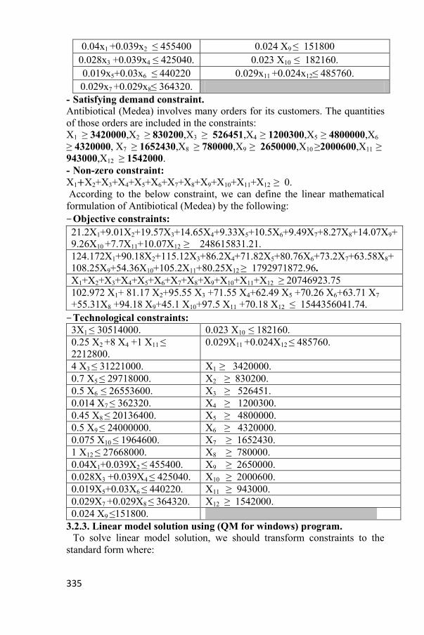
335
0.024 X9 ≤ 151800 0.04x1 +0.039x2 ≤ 455400
0.023 X10 ≤ 182160. 0.028x3 +0.039x4 ≤ 425040.
0.029x11 +0.024x12≤ 485760. 0.019x5+0.03x6 ≤ 440220
0.029x7 +0.029x8≤ 364320.
- Satisfying demand constraint.
Antibiotical (Medea) involves many orders for its customers. The quantities
of those orders are included in the constraints:
X1 ≥ 3420000,X2 ≥ 830200,X3 ≥ 526451,X4 ≥ 1200300,X5 ≥ 4800000,X6
≥ 4320000, X7 ≥ 1652430,X8 ≥ 780000,X9 ≥ 2650000,X10 ≥2000600,X11 ≥
943000,X12 ≥ 1542000.
- Non-zero constraint:
X1+X2+X3+X4+X5+X6+X7+X8+X9+X10+X11+X12 ≥ 0.
According to the below constraint, we can define the linear mathematical
formulation of Antibiotical (Medea) by the following:
- Objective constraints:
- Technological constraints:
3X1 ≤ 30514000. 0.023 X10 ≤ 182160.
0.25 X2 +8 X4 +1 X11 ≤
2212800.
0.029X11 +0.024X12 ≤ 485760.
4 X3 ≤ 31221000. X1 ≥ 3420000.
0.7 X5 ≤ 29718000. X2 ≥ 830200.
0.5 X6 ≤ 26553600. X3 ≥ 526451.
0.014 X7 ≤ 362320. X4 ≥ 1200300.
0.45 X8 ≤ 20136400. X5 ≥ 4800000.
0.5 X9 ≤ 24000000. X6 ≥ 4320000.
0.075 X10 ≤ 1964600. X7 ≥ 1652430.
1 X12 ≤ 27668000. X8 ≥ 780000.
0.04X1+0.039X2 ≤ 455400. X9 ≥ 2650000.
0.028X3 +0.039X4 ≤ 425040. X10 ≥ 2000600.
0.019X5+0.03X6 ≤ 440220. X11 ≥ 943000.
0.029X7 +0.029X8 ≤ 364320. X12 ≥ 1542000.
0.024 X9 ≤151800.
3.2.3. Linear model solution using (QM for windows) program.
To solve linear model solution, we should transform constraints to the
standard form where:
21.2X1+9.01X2+19.57X3+14.65X4+9.33X5+10.5X6+9.49X7+8.27X8+14.07X9+
9.26X10 +7.7X11+10.07X12 ≥ 248615831.21.
124.172X1+90.18X2+115.12X3+86.2X4+71.82X5+80.76X6+73.2X7+63.58X8+
108.25X9+54.36X10+105.2X11+80.25X12 ≥ 1792971872.96.
X1+X2+X3+X4+X5+X6+X7+X8+X9+X10+X11+X12 ≥ 20746923.75
102.972 X1+ 81.17 X2+95.55 X3 +71.55 X4+62.49 X5 +70.26 X6+63.71 X7
+55.31X8 +94.18 X9+45.1 X10+97.5 X11 +70.18 X12 ≤ 1544356041.74.

336
- Constraints (1-4): the objective constraints are classed by priority, we
enter the deviation variable as the following:
- In the case of: objective constraints (≤), we should enter the deviation
variable which maximize (d+) to minimize objective function.
- In the case of: objective constraints (≥) we should enter the deviation
variable which (d-) to minimize objective function.
- The constraint (5-29): it is technological constraints transformed into
function such as resources constraints in the linear programming.
Whereas:
Min Z= dˉ1+d
ˉ2+d
ˉ3+ d
+4.
21.2X1+9.01X2+19.57X3+14.65X4+9.33X5+10.5X6+9.49X7+8.27X8+14.07X
9+9.26X10+7.7X11+10.07X12+ dˉ1- d
+1=248615831.21.
124.172X1+90.18X2+115.12X3+86.2X4+71.82X5+80.76X6+73.2X7+63.58X8
+108.25X9+54.36X10+105.2X11+80.25X12+dˉ2 - d
+2=1792971872.96.
X1+X2+X3+X4+X5+X 6+ X7+ X8+ X9+ X10 +X11 +X12 + dˉ3-d
+3=20746923.23
102.972X1+ 81.17 X2+95.55X3 +71.55 X4+62.49X5 +70.26 X6+63.71X7
+55.31X8+94.18X9+45.1X10 +97.5X11 +70.18 X12+ dˉ4-d
+4= 1544356041.74.
3 X1 +S1= 30514000.
0.25 X2 +8 X4+1X11 +S2=22128000
4 X3+S3=31221000.
0.7 X5 +S4=29718000.
0.5 X6 +S5 = 26553600.
0.014 X7+S6 = 362320.
0.45 X8+S7 =20136400.
0.5 X9 +S8=24000000.
0.075 X10+S9=1964600.
1 X12 +S10= 27668000.
0.04X1 +0.039X2 + S11= 455400.
0.028X3+0.039X4 +S12=425040.
0.019X5+0.03X6 + S13= 440220.
0.029X7 +0.029X8+S14=364320.
0.024 X9 +S15=151800.
0.023 X10 +S16 =182160.
0.029X11 + 0.024X12+ S17 = 485760.
X1 –S18 = 3420000
X2 –S19= 830200
X3 – S20= 526451
X4 – S21 = 1200300
X5 – S22 = 4800000
X6 – S23 = 4320000
X7 – S24= 1652430
X8 – S25 = 780000
X9 – S26= 2650000
X10 – S27 =2000600
X11 – S28 = 943000

337
X12 – S29= 1542000
X1+X2+X3+X4+X5+X6+X7+X8+X9+X10+X11+ X12≥ 0 .
3.2.4. Reading and analysis of linear programming with multiple
objectives using (QM for windows)
3.2.4.1. Analysis of decisions variables:
According to the typical solution table (index 01) we find the following
quantities:
X1 = 3420000, X2 = 830200, X3 = 526451, X4 = 1200300, X5 = 4800000,
X6 = 4320000, X7 =1652430, X8 =780000, X9 =2650000, X10 =2000600, X11 = 943000, X12 = 1542000.
3.2.4.2. Psychiatry of objective value:
- Maximize profit objective: The profit plan of each product and its total
profit summarized in the following table:
Table 05: Production quantity and total profit according to the proposed
Source: data of program outputs.
Through the previous table, we can observe that proposed profit is more
than target profit, and the deviation obtained is a positive deviation, thus the
typical solution is about: 50129730 AD. Here we can say that profit of the
Antibiotical (Medea) will be increases in the case of using the proposed plan
presented by 50129730 AD, it is about 20.16%.
- Maximize revenues objective: We can describe the revenues plan for each
product in the following table:
Table6: Obtained production quantity and obtained revenues according
to the proposed plan.
product
Proposed
production
quantity
Profit unit (AD) Proposed profit
X1 3420000 21.2 72504000
X2 830200 9.01 7480102
X3 526451 19.57 10302646.07
X4 1200300 14.65 17584395
X5 4800000 9.33 44784000
X6 4320222 10.5 45362331
X7 1652430 9.49 15681560.7
X8 780000 8.27 6450600
X9 2650000 14.07 37287047.7
X10 2000600 9.26 18523704
X11 943000 7.7 7261100
X12 1542000 10.07 15507800
total 24663113 - 298729286.5
Product Proposed production
quantity Unit price
Proposed
Revenues
X1 3420000 124.172 424668240
X2 830200 90.18 74867436
X3 526451 115.12 60605039.12

338
Sourc
e:
data
of
progr
am
outpu
ts.
The analysis of data below can describe a positive deviation in revenues,
where the proposed revenues are more than target revenues. The typical
solution presented by: 353357300 AD.
There is a possibility of revenues increase in the same of using the proposal
plan, it is about 19.70%.
- Maximize production quantity objective: The quantity proposed
production for each product and total production is described in the
following table:
Table 7: Production quantity according to the proposed plan
Product Proposed
production quantity Product
Proposed
production
quantity
X1 3420000 X7 1652430
X2 830200 X8 780000
X3 526451 X9 2650000
X4 1200300 X10 2000600
X5 4800000 X11 943000
X6 4320222 X12 1542000
total 24663113
Source: data of program outputs
We can observe a positive deviation where the proposed plan was more than
the target quantity.
The deviation equal 3917860 AD, 18,87%, it is the result of the increase in
the production quantities X1,X2,X3,X4,X5,X6,X7,X8,X9,X10,X11,X12 in 2015
according to 2014. It means that the proposed plan is the most efficient.
- Minimize production cost objective: The following table explains the
proposed production plan for each product related to the total costs.
X4 1200300 86.2 103465860
X5 4800000 71.82 344736000
X6 4320222 80.76 348901128.7
X7 1652430 73.2 120957876
X8 780000 63.58 49592400
X9 2650000 108.25 286874407.5
X10 2000600 54.36 108741744
X11 943000 105.2 99203600
X12 1542000 80.25 123585000
total 24663113 - 2146198731
Product Proposed
production quantity Cost price (AD)
Proposed
production costs
X1 3420000 102.972 352164240
X2 830200 81.17 67387334
X3 526451 95.55 50310992.55
X4 1200300 71.55 85881465
X5 4800000 62.49 299952000
X6 4320222 70.26 303538797.7
X7 1652430 63.71 105276315.3

339
Tabl
e 08 :
prod
uctio
n
quan
tity and costs according to proposed plan.
Source: data of program outputs
The production cost in the proposed plan was 1847478044, the deviation
was negative, where the production cost increase above the allowed amount
1544356000 AD, with difference of 303122044 according to the typical
solution table.
3.2.4.3. Technical constraints value analysis.
These constraints divided into the following:
- Active substance constraints: The typical solution table describes [dˉ
(rowi)] as the non used active substance quantities (b1, b2, b3……….b10)
they are the following:
(20254000),(11375050),(29115200),(26358000),(24393600),(339186),
(19785400), (22675000),(1814570),(26126000).
The exploitation of the following quantities:
(12260000), (10752950), (2105800), (3360000), (2160000), (23134),
(351000), (1325000), (150030),(1542000).
- Production capacity constraints: The corresponding values of the
available production capacity presented by the column [d+(rowi)] which is
nil(zero), whereas it is not zero in the column [dˉ(rowi)] .
In other word, there is an available capacity which is not exploited in the
production lines.
The excess production capacity in the production lines:
286222.2 AD in the first production line, 363487.7 AD in the second
production line, 219420 AD in the third production line, 293779.5 AD in the
fourth productive line, 88200 AD in the fifth productive line, 136150.8 in the
sixth productive line and 421405 AD in the seventh production line.
The decision maker must rethink how to exploit the excess in production
capacity in order to improve the Antibiotical (Medea) profit.
- Satisfying (fulfilling) demand constraints: There is a zero (nil)
corresponding values represented by the column [dˉ(rowi)], it means we
have a decrease in the quantity demanded presented by [d+(rowi)], that is to
say no increase in the quantity demanded.
4. Sensitivity Analysis: To analyze the linear programming with multiple
objectives sensitivity, we will mention the following points:
4.1. Effect of objective levels variations:
Through this study we find that antibiotical (Medea) determines four 04
main objectives in the same time:
X8 780000 55.31 43141800
X9 2650000 94.18 249587359.8
X10 2000600 45.1 90218040
X11 943000 97.5 91942500
X12 1542000 70.18 108077200
total 24663113 - 1847478044

340
- Non basic deviation variable: From the typical solution table we can
determine the non basic deviation variables which appeared with nil (zero)
values in the typical solution table: d-1, d
-2, d
-3, d
-4.
There is a possibility to determine the maximum and minimum change in the
following table:
Table09: Maximum and minimum variation for the non basic variables Objective Non basic
variable
Minimum
possible
Maximum
possible
1 dˉ1 -1 0
2 dˉ2 -1 0
3 dˉ3 -1 0
4 dˉ4 -1 0
Source: data of program outputs
From the table 9, we observe: without any impact on the production plan,
the antibiotical (Medea) can change the target values under the allowed
limits for each objective.
- The basic deviation variables: The typical solution table indicates that the
variable d+
1 appeared as a positive deviation presented by 50129730 cans,
that is to say the total production increase by 50129730 cans, or be decrease
any amount without any changes under the typical case in the basic variables
in the typical solution table: d+
2, d+
3, and d+
4.
4.2. The relative exchange between objectives: Although the linear
programming with multiple objectives is not the way to exchange objective,
but there is a possibility to determine the relative values of different
objectives by analyzing and testing the last solution table, because it will
make decision maker able to get the important data and the flexibility to
make the best decisions.
The relative exchange between objectives means the determination of the
impact caused by decreasing negative deviation to the low priority objective
than the negative deviation to the top priority objective.
Through the typical solution table, we find the negative deviation for the
fourth objective (minimize cost of production) represented by 303227800
cans. It is possible to decrease this deviation?
From the fourth objective, we can say that there is possibility to improve
the objective function. through selecting the variable d+
4 as anon basic
variable, where it takes a positive exchange (+1), this selection will decrease
deviation in this objective to a less value.
In the case of d+
4 is non basic variable, its value equal the value of
achieving objective with the top priority (maximizing production quantity
objective (objective 03). It means that for any unit of decrease from the
maximizing production quantity objective. We get a decrease in production
costs by one single unit of money. The exchange between the two objectives
(cost of production and quantity of production) is one single unit of money.

341
4.3. Order priorities variation: Objectives for the decisions maker haven’t
the same importance, with different levels from one objective to another.
Decision maker can’t decide definitely about the objectives priority, where
he rethinks about priority orders variation due to the new changes in this
enterprise environment or the changes in objectives.
According to this big importance, we can explain it by reordering
objectives for this enterprise antibiotical (Medea) as the following:
Table 10: typical solution table after the reordering of objectives
Source: data of program outputs
Through the previous table, we find that typical solution may have a small
change after reordering objectives, that is to say after changing priorities the
typical table will be change to a new production variety. This can make
decisions maker more carefully in ordering objectives.
Study results:
Antibiotical (Medea) can increase its production variety, according to the
same period but with minimizing deviation to the less possible value.
After analyzing objectives levels, linear programming with multiple
objectives presents the distinct results in the antibiotical (Medea). This way
can determine the typical solution which reconcile between objectives and
its efficiency. Antibiotical (Medea) plan to produce large quantities of
production to get more profit in order to obtain more revenues under the
constraint of high costs.
Through sensitivity analysis, we determine different deviation change for
the non basic variables in the mathematical model, this result allows the
decision maker to change the target values (rising/reducing), without
affecting the typical production variety.
Study recommendation:
There is a need to use the linear programming with multiple objective and
the quantitative tools, especially operational research, moreover the
coordination with universities to solve enterprise problems.
Antibiotical (Medea) could follow the proposed plan because it affords
more advantages.
Linear programming with multiple objectives describes the non used
production capacity; there is a need to reconsider it to realize enterprise
objectives.
References: 1
- Bichino J., Elliot B., operations management, N.Y, Black-Well Publishers
ltd, 2008, P151.

342
2 - Bunn, D., Applied decision analysis, N.Y.Me Graw- Hill, 2002, p230.
3 - Hiller F., Liberman .G, Introduction to management science, California,
H.D, 2003, P 153. 4 - Andersson D.R, Sweeney D .j,An Introduction to management science,
Quantitative approaches to decision making Cincinnati, S.w.college pub,
2001, P 124. 5 - Render B., Quantitative analysis for management, Prince Hall, N.Y, 2000,
p189. 6 - Thomas.R, Quantitative methods for business studies, Prince Hall, N.Y,
2003, p171. 7 - Dhénin J.F, Fournie B, Initiation à l’économie de l’entreprise, Ed .Breal,
paris, 1998, P175.
8 - Minoux M., Programmation mathématique, théorie ET algorithmes,
Dunod, 2002, P251. 9
- Eppen G.D., Gould F.J, Quantitative concepts for management: decision
making without algorithms .Englewood Cliffs, N.J, Prentice H.I, 2002, P146. 10
- Lee, S.M, Olson D. L., in multicriteria decision making, advances in
MCDM models, Algorithms, Theory and Applications, Hanne (Eds), kluwer
académie publishers, Boston, 2001, p842. 11
-Gordon G, Pressman I., Quantitative decision making for business.
Englewood Cliffs, N. J, Prentice H.I, 2001, P202. 12
-Wagner H.M, Principles of operations research: with applications to
Managerial decisions, Englewood Cliffs, N.J, Prentice Hall, 2001, P258. 13
- Charnes A, Cooper w, A Goal programming model for media planning
management science, N.Y, Prentice H, 2003, p 425- 427. 14
- Martel. J & Aouni, Incorporating the decision Marker’s preferences in
the Goal Programming model, Journal of the operation research society,
2003, p1122- 1124. 15
- Saaty T.L, Mathematical methods of operations research, N.Y., MC
Graw– Hill, 2002, P205.