linear programming - raj...
TRANSCRIPT
LINEAR PROGRAMMING- LECTURE NOTES FOR QTM PAPER OF BBE (H), DELHI UNIVERSITY (2013-14)
1 RAJKUMAR, Assistant Professor, College of Vocational Studies, Delhi University. http://rajkumar2850.weebly.com/, 9910232006
LINEAR PROGRAMMING
All organizations, whether large or small, need optimal utilization of their scarce or limited
resources to achieve certain objectives. Scarce resources may be money, manpower, material,
machine capacity, technology, time etc. In order to achieve best possible result(s) with the
available resources, the decision maker must understand all facts about the organization activities
and the relationships governing among chosen activities and its outcome. The desired outcome
may be measured in term of profits, time, return on investment, costs, etc.
Of all the well known operations research models, linear programming is the most popular and
most widely applied technique of mathematical programming. Basically, linear programming is a
deterministic mathematical technique which involves the allocation of scarce or limited
resources in an optimal manner on the basis of a given criterion of optimality. Frequently, the
criterion of optimality is profits, costs, return on investment, time, distance, etc.
George B Dantzig, while working with US Air Force during WWII in 1947, developed the
technique of linear planning. LP was developed as a technique to achieve the best plan out of
different plans for achieving the goal through various activities like procurement, recruitment,
maintenance, etc.
In linear programming decisions are made under certainty i.e. information on available resource
and relationships between variables are known. Therefore actions chosen will invariably lead to
optimal or nearly optimal results. In sum, we can say that linear programming provides a
quantitative basis to assist a decision maker in selection of the most effective and desirable
course of action from a given number of available alternatives to achieve the result in an optimal
manner.
Standard form of the model
In the class

LINEAR PROGRAMMING- LECTURE NOTES FOR QTM PAPER OF BBE (H), DELHI UNIVERSITY (2013-14)
2 RAJKUMAR, Assistant Professor, College of Vocational Studies, Delhi University. http://rajkumar2850.weebly.com/, 9910232006
Basic terminology, requirements, assumptions, advantages and limitations-
Basic terminology-
Linear- the word linear used to describe the relationships among two or more variables which are
directly or precisely proportional.
Programming- the word ‘programming’ means that the decisions are taken systematically by
adopting various alternative courses of actions.
Optimal- A program is optimal if it maximises or minimise some measure or criterion of
effectiveness such as profit, cost, or sales. The term ‘limited’ refers to the availability of
resources during planning horizon.
A feasible solution is a solution for which all the constraints are satisfied
An infeasible solution is a solution for which at least one constraint is violated
The feasible region is the collection of all feasible solutions
An optimal solution is a feasible solution that has the most favourable value of the objective
function
The most favourable value is the largest value if the objective function is to be maximised,
whereas it is smallest value if the objective function is to be minimised
A corner point feasible is a solution that lies at a corner of the feasible region.
Relationship between optimal solution and CPF solutions- consider any linear programming
problem with feasible solutions and a bounded feasible region. The problem must possess CPF
solution and at least one optimal solution. Furthermore, the best solution must be an optimal
solution. Thus, if a problem has exactly one optimal solution, it must be a CPF solution. If the
problem has multiple optimal solutions, at least two must be CPF solutions.
Basic requirements-
LINEAR PROGRAMMING- LECTURE NOTES FOR QTM PAPER OF BBE (H), DELHI UNIVERSITY (2013-14)
3 RAJKUMAR, Assistant Professor, College of Vocational Studies, Delhi University. http://rajkumar2850.weebly.com/, 9910232006
(a) Decision variables and their relationship
(b) Objective function
(c) Constraints
(d) Alternative courses of action
(e) Non-negative restriction
(f) Linearity
Basic assumptions
All assumptions of linear programming actually are implicit in the model formulation. In
particular, from a mathematical viewpoint, the assumptions simply are that the model must have
a linear objective function subject to linear constraints. However, from a model viewpoint, these
mathematical properties of a linear porgamming model imply that certain assumptions must hold
about the activities and data of the problem being modelled, including assumptions about the
effect of varying the levels of the activities.
(a) Proportionality- the contribution of each activity to the value of the objective function is
proportional to the level of the activity xj . Similarly, the contribution of each activity to
the left hand side of each functional constraint is proportional to the level of the activity
xj . consequently, this assumption rules out any exponent other than 1 for any variable in
any term of any function in linear programming model.
In case of violation of this assumption, we will use the nonlinear
programming. Furthermore, if the assumption is violated only because of start up costs,
there is extension of linear programming (mixed integer programming) that can be used.
(b) Divisibility (or continuity)
(c) Additivity- every function in a linear programming model (whether the objective function
or the function on the left hand side of a functional constraint) is the sum of the
individual contribution of the respective activities.
Although the proportionality assumption rules out exponents other than 1, it does
not prohibit cross product terms (terms involving the product of two or more variables).
The additivity assumption does rule out this latter possibility.
(d) Deterministic coefficients (or parameters)
LINEAR PROGRAMMING- LECTURE NOTES FOR QTM PAPER OF BBE (H), DELHI UNIVERSITY (2013-14)
4 RAJKUMAR, Assistant Professor, College of Vocational Studies, Delhi University. http://rajkumar2850.weebly.com/, 9910232006
Advantages of Linear programming
See reference book
Limitations of Linear programming
See reference book
**************
We will cover following two methods of LPP in our course.
1. Graphical Method
2. Simplex Method- In Simplex Method, we will discuss single constraint (all slack variable
method) and mixed constraint (Big M and two phase method).
Graphical Method
So far we have learnt how to construct a mathematical model for a linear programming problem.
If we can find the values of the decision variables x1, x2, x3, ..... xn, which can optimize
(maximize or minimize) the objective function Z, then we say that these values of xi are the
optimal solution of the Linear Program (LP).
The graphical method is applicable to solve the LPP involving two decision variables x1, and x2,
we usually take these decision variables as x, y instead of x1, x2. To solve an LP, the graphical
method includes two major steps.
a) The determination of the solution space that defines the feasible solution. Note that the
set of values of the variable x1, x2, x3,....xn which satisfy all the constraints and also the
non-negative conditions is called the feasible solution of the LP.
b) The determination of the optimal solution from the feasible region.
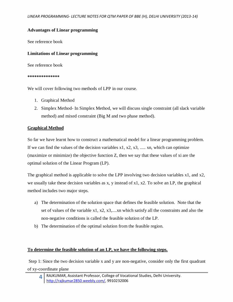
To determine the feasible solution of an LP, we have the following steps.
Step 1: Since the two decision variable x and y are non-negative, consider only the first quadrant
of xy-coordinate plane

LINEAR PROGRAMMING- LECTURE NOTES FOR QTM PAPER OF BBE (H), DELHI UNIVERSITY (2013-14)
5 RAJKUMAR, Assistant Professor, College of Vocational Studies, Delhi University. http://rajkumar2850.weebly.com/, 9910232006
Step 2 each constraint is of the form ax + by ≤ c or ax + by ≥ c
Draw the line for each constraint with equality sign i.e. ax + by = c
Step 3: Corresponding to each constant, we obtain a shaded region. The intersection of all these
shaded regions is the feasible region or feasible solution of the LP.
We can explain graphical method by using example.
There are two techniques to find the optimal solution of an LPP.
1. Corner Point Method
2. ISO-PROFIT (OR ISO COST) Method
Corner Point Method
The optimal solution to a LPP, if it exists, occurs at the corners of the feasible region.
The method includes the following steps
Step 1: Find the feasible region of the LLP.
Step 2: Find the co-ordinates of each vertex of the feasible region. These co-ordinates can be
obtained from the graph or by solving the equation of the lines.
Step 3: At each vertex (corner point) compute the value of the objective function.
Step 4: Identify the corner point at which the value of the objective function is maximum (or
minimum depending on the LP)
The co-ordinates of this vertex is the optimal solution and the value of Z is the optimal value
Example -------------in the class
If an LPP has many constraints, then it may be long and tedious to find all the corners of the
feasible region. There is another alternate and more general method to find the optimal solution
of an LP, known as 'ISO profit or ISO cost method'
ISO- PROFIT (OR ISO-COST) METHOD

LINEAR PROGRAMMING- LECTURE NOTES FOR QTM PAPER OF BBE (H), DELHI UNIVERSITY (2013-14)
6 RAJKUMAR, Assistant Professor, College of Vocational Studies, Delhi University. http://rajkumar2850.weebly.com/, 9910232006
Method of Solving Linear Programming Problems
Suppose the LPP is to
Maximize Z = c1x1 + c2x2
Subject to the constraints
a11x1 + a12x2 ≤ b1
a21x1 + a22x2 ≤ b2
This method of optimization involves the following method.
Step 1: Draw the half planes of all the constraints
Step 2: Shade the intersection of all the half planes which is the feasible region.
Step 3: Since the objective function is Z = c1x1 + c2x2 draw a dotted line for the equation Z = c1x1
+ c2x2 = k, where k is any constant. Sometimes it is convenient to take k as the LCM of a and b.
Step 4: To maximize Z draw a line parallel to Z = c1x1 + c2x2 = k and farthest from the origin.
This line should contain at least one point of the feasible region. Find the coordinates of this
point by solving the equations of the lines on which it lies.
To minimize Z draw a line parallel to Z = c1x1 + c2x2 = k and nearest to the origin. This line
should contain at least one point of the feasible region. Find the co-ordinates of this point by
solving the equation of the line on which it lies.
Step 5: If (x1, x2) is the point found in step 4, then x1, x2, is the optimal solution of the LPP.
Numerical example----------------- in the class
Max Z = 3 x1 + 5 x2 (1)

LINEAR PROGRAMMING- LECTURE NOTES FOR QTM PAPER OF BBE (H), DELHI UNIVERSITY (2013-14)
7 RAJKUMAR, Assistant Professor, College of Vocational Studies, Delhi University. http://rajkumar2850.weebly.com/, 9910232006
Subject to the constraints
x1 ≤ 4
2x2 ≤ 12
3x1 + 2x2 ≤ 18
Simplex Method
It was observed in the graphical approach to the solution of such problem that, in a given
situation, the feasible region is determined by the set of constraints given in the problem while
the objective function locates the optimal point- the one that maximise or minimises, as the case
may be. Although this method is very efficient in developing the conceptual framework
necessary for fully understanding the linear programming process, it suffers from the great
limitation that it can handle problem involving only two decision variables. In the real world
situations, we frequently encounter cases where more than two variables are involved and,
therefore, look for a method that can handle them. The Simplex method provides an efficient
technique which can be applied for solving LPPs of any magnitude- involving two or more
decision variables.
The simplex algorithm is an iterative procedure for finding, in a systematic manner, the optimal
solution to a linear programming problem. Simplex method is developed by George Dantzig in
1947.
Key solution concepts in Simplex Method
1. The simplex method focuses solely on CPF solutions. For any problem with at least one
optimal solution, finding one requires only finding best CPF solution.
2. The simplex method is an iterative algorithm with the following structure
a. Initialization
b. Optimality test- is the current CPF solution optimal? If yes- stop, if no then go for
iteration

LINEAR PROGRAMMING- LECTURE NOTES FOR QTM PAPER OF BBE (H), DELHI UNIVERSITY (2013-14)
8 RAJKUMAR, Assistant Professor, College of Vocational Studies, Delhi University. http://rajkumar2850.weebly.com/, 9910232006
c. Iteration- performs an iteration to find a better CPF solution.
3. Whenever possible, the initialisation of the simplex method chooses the origin (all
decision variables equal to zero) to be the initial CPF solution.
4. Given a CPF solution, it is much quicker computationally to gather information about its
adjacent CPF solutions than about other CPF solution. Therefore, each time the simplex
method performs an iteration to move from the current CPF solution to a better one, it
always chooses a CPF solution that is adjacent to the current one. No other CPF solutions
are considered. Consequently, the entire path followed to eventually reach an optimal
solution is along the edges of the feasible region.
5. After the current CPF solution is identified, the simplex method examines each of the
edges of the feasible region that emanate from this CPF solution. Each of these edges
leads to an adjacent CPF solution at the other end, but the simplex method does not even
take the time to solve for the adjacent CPF solution. Instead, it simply identifies the rate
of improvement in Z that would be obtained by moving along the edge. Among the edges
with a positive rate of improvement in Z, it then chooses to move along the one with the
largest rate of improvement in Z. The iteration is completed by first solving for the
adjacent CPF solution at the other end of this one edge and then relabeling this adjacent
CPF solution as the current CPF solution for the optimality test and (if needed) the next
iteration.
6. Solution concept 5 describes how the simplex method examines each of the edges of the
feasible region that emanate from the current CPF solution. This examination of an edge
leads to quickly identifying the rate of improvement in Z that would be obtained by
moving along the edge toward the adjacent CPF solution at the other end. A posit ive rate
of improvement in Z implies that the adjacent CPF solution is better than the current CPF
solution, whereas a negative rate of improvement in Z implies that the adjacent CPF
solution is worse. Therefore, the optimality test consists simply of checking whether any
of the edges give a positive rate of improvement in Z. If none do, then the current CPF
solution is optimal.

LINEAR PROGRAMMING- LECTURE NOTES FOR QTM PAPER OF BBE (H), DELHI UNIVERSITY (2013-14)
9 RAJKUMAR, Assistant Professor, College of Vocational Studies, Delhi University. http://rajkumar2850.weebly.com/, 9910232006
The Algebra of the Simplex Method
Suppose that the Linear programming problem is given as following
Z = c1x1 + c2x2
Subject
a11 x1 + a12x2 ≤ b1
a21x1 + a22 x2 ≤ b2
We can explain the Algebra of the simplex method by following fig.
We can explain the simplex method by using proto-type example of LPP
The Linear programming problem is given
Initialisation (Using
Slack, surplus, Artificial
variable as per
required)
Optimality Test
Yes
No
Determine Leaving basic
variable and Entering basic
variable
Update the
simplex table
LINEAR PROGRAMMING- LECTURE NOTES FOR QTM PAPER OF BBE (H), DELHI UNIVERSITY (2013-14)
10 RAJKUMAR, Assistant Professor, College of Vocational Studies, Delhi University. http://rajkumar2850.weebly.com/, 9910232006
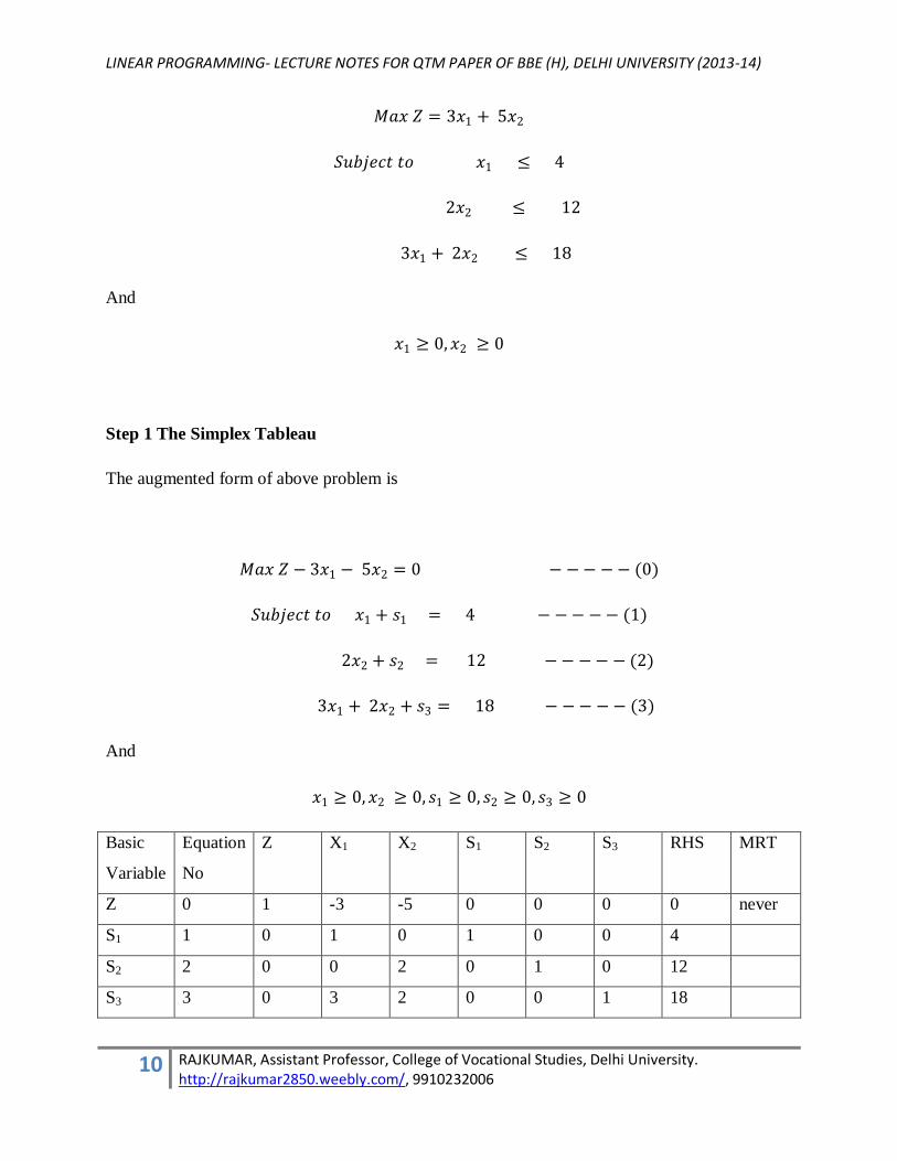
𝑀𝑎𝑥 𝑍 = 3𝑥1 + 5𝑥2
𝑆𝑢𝑏𝑗𝑒𝑐𝑡 𝑡𝑜 𝑥1 ≤ 4
2𝑥2 ≤ 12
3𝑥1 + 2𝑥2 ≤ 18
And
𝑥1 ≥ 0,𝑥2 ≥ 0
Step 1 The Simplex Tableau
The augmented form of above problem is
𝑀𝑎𝑥 𝑍 − 3𝑥1 − 5𝑥2 = 0 − −− −− (0)
𝑆𝑢𝑏𝑗𝑒𝑐𝑡 𝑡𝑜 𝑥1 + 𝑠1 = 4 − −− −− (1)
2𝑥2 + 𝑠2 = 12 −− −− − (2)
3𝑥1 + 2𝑥2 + 𝑠3 = 18 − −− −− (3)
And
𝑥1 ≥ 0,𝑥2 ≥ 0, 𝑠1 ≥ 0, 𝑠2 ≥ 0, 𝑠3 ≥ 0
Basic
Variable
Equation
No
Z X1 X2 S1 S2 S3 RHS MRT
Z 0 1 -3 -5 0 0 0 0 never
S1 1 0 1 0 1 0 0 4
S2 2 0 0 2 0 1 0 12
S3 3 0 3 2 0 0 1 18

LINEAR PROGRAMMING- LECTURE NOTES FOR QTM PAPER OF BBE (H), DELHI UNIVERSITY (2013-14)
11 RAJKUMAR, Assistant Professor, College of Vocational Studies, Delhi University. http://rajkumar2850.weebly.com/, 9910232006
The MRT column is for the minimum ration test. A tableau in proper form has these
characteristics
1. Exactly one basic variable per equation
2. The coefficient of the basic variable is always exactly +1 and the coefficient above and
below the basic variable in the same column are all 0
3. Z is treated as the basic variable for the objective function row (equation 0)
A big advantage of proper form is that you can always read the current solution directly from the
tableau. This is because there is exactly one basic variable per row, and the coefficient of that
variable is +1. All the other variables in the row are nonbasic (set to zero), so the value of any
variable is just given by the value shown in the RHS column.
Step 2: Are we optimal yet?
If the coefficients of z row are non-negative then current solution is optimum (remember
objective function is 𝑍 − 3𝑥1 − 5𝑥2 = 0. If any coefficient of z row is negative then current
solution is not optimum.
Step 3: Select the entering basic variable
Choose the variable in the objective function row that has the most negative value as the
entering basic variable.
We can choose only one variable as entering basic variable at one time (see point no 5 in key
concepts in simplex)
Step 4: Select the leaving basic variable
The minimum ratio test is used to determine the leaving basic variable. MRT determines which
constraint most limits the increase in the value of the entering basic variable. The most limiting
constraint is one whose basic variable is driven to zero first as the entering basic variable
increases in value.
For the minimum ratio test, look only at the entries in the pivot column (the column for the
entering basic variable) for the constraint rows, and calculate

LINEAR PROGRAMMING- LECTURE NOTES FOR QTM PAPER OF BBE (H), DELHI UNIVERSITY (2013-14)
12 RAJKUMAR, Assistant Professor, College of Vocational Studies, Delhi University. http://rajkumar2850.weebly.com/, 9910232006
(RHS)/(Coefficient of entering basic variable)
There are two special cases
If the coefficient of the entering basic variable is zero: enter no limit in the MRT column
If the coefficient of the entering basic variable is negative: enter no limit in the minimum
ration test column.
The MRT is never applied to the objective function row. Reason- the objective function row is
not a constraint, so it can never limit the increase in the value of the entering basic variable.
As usual in the MRT, the leaving basic variable is associated with the row that has the minimum
value of the ratio test. This row is called the pivot row.
Basic
Variable
Equation
No
Z X1 X2
(Entering
basic
variable)
S1 S2 S3 RHS MRT
Z 0 1 -3 -5 0 0 0 0 never
S1 1 0 1 0 1 0 0 4 No limit
S2 2 0 0 2 0 1 0 12 6
(Minimum)
S3 3 0 3 2 0 0 1 18 9
Step 5: Update the tableau
As we discussed in the class
LINEAR PROGRAMMING- LECTURE NOTES FOR QTM PAPER OF BBE (H), DELHI UNIVERSITY (2013-14)
13 RAJKUMAR, Assistant Professor, College of Vocational Studies, Delhi University. http://rajkumar2850.weebly.com/, 9910232006
Special Cases
Tie for the entering basic variable
Suppose that there are two or more nonbasic variables that have the same most negative value in
the objective function row.
𝑍 = 15𝑥1 + 15𝑥2
this means that both x1 and x2, if allowed to become basic and increase in value, would increase
Z at the same rate.
So how to handle this situation? Simple: choose the entering basic variable arbitrarily from
among those tied at the most negative value
Tie for the leaving basic variable:
Again, simply choose arbitrarily. The variable that is not chosed as the leaving basic variable
will remain basic, but will have a calculated value of zero. In contrast, the variable chosen as the
leaving basic variable will of course be forced to zero by simplex. Both variable must be zero
simultaneously because both constraints are active at that point; it is just that simplex only needs
one of them to define the basic feasible solution.
When there is a tie for the leaving basic variable as we have described, the basic feasible solution
defined what is known as a degenerate solution.

LINEAR PROGRAMMING- LECTURE NOTES FOR QTM PAPER OF BBE (H), DELHI UNIVERSITY (2013-14)
14 RAJKUMAR, Assistant Professor, College of Vocational Studies, Delhi University. http://rajkumar2850.weebly.com/, 9910232006
Linear Programming-Mixed constraints
In above section, we looked at linear programming problems that occurred in standard form. The
constraints for the maximization problems all involved inequalities, and the constraints for the
minimization problems all involved inequalities.
Linear programming problems for which the constraints involve both types of inequalities are
called mixed-constraint problems. For instance, consider the following linear programming
problem.
Mixed-Constraint Problem: Find the maximum value of
Where x1 ≥ 0, x2 ≥ 0, x3 ≥ 0 and Since this is a maximization problem, we would expect each
of the inequalities in the set of constraints to involve . Moreover, since the first inequality does
involve , we can add a slack variable to form the following equation.
For the other two inequalities, we must introduce a new type of variable, called a surplus
variable, as follows.

LINEAR PROGRAMMING- LECTURE NOTES FOR QTM PAPER OF BBE (H), DELHI UNIVERSITY (2013-14)
15 RAJKUMAR, Assistant Professor, College of Vocational Studies, Delhi University. http://rajkumar2850.weebly.com/, 9910232006
Notice that surplus variables are subtracted from(not added to) their inequalities. We call s2 and
s3 surplus variables because they represent the amount that the left side of the inequality exceeds
the right side. Surplus variables must be nonnegative.
Now, to solve the linear programming problem, we form an initial simplex tableau as follows.
Basic
Variable
Equation
no
Z X1 X2 X3 S1 S2 S3 RHS MRT
Z 0 1 -1 -1 -2 0 0 0 0 Never
S1 1 0 2 1 1 1 0 0 50
S2 2 0 2 1 0 0 -1 0 36
S3 3 0 1 0 1 0 0 -1 10
You will soon discover that solving mixed-constraint problems can be difficult. One reason for
this is that we do not have a convenient feasible solution to begin the simplex method. Note that
the solution represented by the initial tableau above.
is not a feasible solution because the values of the two surplus variables are negative.
In order to start simplex process, we will introduce the artificial variable. We will explain two
methods which uses the artificial variable, namely
1. Big M or M Method
2. Two phase method
Big M method or M Method
Min Z= c1x1 + c2x2

LINEAR PROGRAMMING- LECTURE NOTES FOR QTM PAPER OF BBE (H), DELHI UNIVERSITY (2013-14)
16 RAJKUMAR, Assistant Professor, College of Vocational Studies, Delhi University. http://rajkumar2850.weebly.com/, 9910232006
s.t. a11x1+a12x2 ≥ b1
a21x1+a22x2 ≥ b2
x1, x2 ≥ 0
Augmented form
Min Z= c1x1 + c2x2
s.t. a11x1+a12x2-S1 = b1
a21x1+a22x2-s2 = b2
x1, x2, s1, s2 ≥ 0
S1 and S2 s are called as surplus variables because it is the amount (surplus) by which the left
side of the inequality exceeds the right side.
But this augmented form does not provide the initial basic solution. It is because, simplex
method starts with the case in which all decision variables are zero.
If x1 and x2 are zero then from augmented form
S1=-b1
S2=-b2
So there is violation of non-negative constraint. So to start simplex process, we will use artificial
variable. This variable has no physical meaning in the original problem and is introduced solely
for the purpose of obtaining a basic feasible solution so that we can apply the simplex method.
If equation i does not have a slack (or a variable that can play the role of a slack), an artificial
variable, Ri, is added to form a starting solution similar to the convenient all slack basic solution.
However, because the artificial variables are not part of the original LP model, they are assigned

LINEAR PROGRAMMING- LECTURE NOTES FOR QTM PAPER OF BBE (H), DELHI UNIVERSITY (2013-14)
17 RAJKUMAR, Assistant Professor, College of Vocational Studies, Delhi University. http://rajkumar2850.weebly.com/, 9910232006
a very high penalty in the objective function, thus forcing them (eventually) to equal to zero in
the optimum solution. This will always to be the case if the problem has a feasible solution.
Penalty rule for artificial variables
Step I convert the LPP into equation form by introducing slack and/or surplus variables as the
case may be.
Step II Introduce non negative variables to the left hand side of all the constraints of ≥ or = type.
These variables are called artificial variables. The purpose of introducing artificial variables is
just to obtain an initial basic feasible solution. In order to get rid of the artificial variables in the
final optimum iteration, we assign a very large penalty- M, in maximisation problems to the
artificial variables in the objective function.
Step III Solve the modified LPP by simplex method. While making iteration by this method one
of the following three cases may arise
(a) If no artificial variable remains in the basis, and the optimal condition is satisfied,
then the current solution is an optimal basic feasible solution.
(b) If atleast one artificial variable appears in the basis at zero level (with zero value in
the solution column), and the optimality condition is satisfied, then the current
solution is an optimal basic feasible (though degenerated) solution.
(c) If, at least one artificial variable appears in the basis of non zero level (with positive
value in the solution column), and the optimality condition is satisfied, then the
orginal problem has no feasible solution. The solution satisfies the constraints but
does not optimise the objective function because it contains a very high penalty M
and is termed as the pseudo optimal solution.
While applying the simplex method, whenever an artificial variable happens to leave
the basis, we drop artificial variable and, omit all the entries corresponding to its
column from the simplex table
Step IV Application of simplex method is continued until, either an optimum basic feasible
solution is obtained or there is indication of the existence of an unbounded solution to the given
LPP.

LINEAR PROGRAMMING- LECTURE NOTES FOR QTM PAPER OF BBE (H), DELHI UNIVERSITY (2013-14)
18 RAJKUMAR, Assistant Professor, College of Vocational Studies, Delhi University. http://rajkumar2850.weebly.com/, 9910232006
In simplex table, New z row= old z row -- (M × R1row + R2 row) in case in which we have two
artificial variable in two constraints.
We need to convert z row because all basic variables must be algebraically eliminated from
objective function before the simplex method can either apply the optimality test or find the
entering basic variable. This elimination is necessary so that the negative of the coefficient of
each non basic variable will give the rate at which Z would increase if that nonbasic variable
were to be increased from 0 while adjusting the value of the basic variables accordingly.
The use of the penalty M may not force the artificial variable to zero level in the final simplex
iteration if, the LP does not have a feasible solution (i.e. the constraints are not consistent). In
this case, the final simplex iteration will include at least one artificial variable at a positive level
Theoretically, the application of the M technique implies M → ∞. However, using the computer,
M must be finite but, sufficiently large. How large is “sufficiently large”, is an open question.
Specifically, M should be large enough to act as a penalty. At the same time, it should not be too
large to impair the accuracy of the simplex computations, because of manipulating a mixture of
very large and very small numbers.
Numerical Example
Min Z= 0.4x1 + 0.5x2
s.t 0.3x1+0.1x2 ≤ 2.7
0.5x1+0.5x2 = 6
0.6x1+0.4x2 ≥ 6
x1,x2 ≥ 0
augmented form
Min Z= 0.4x1 + 0.5x2 + MA2 +MA3
s.t 0.3x1+0.1x2 –S1= 2.7

LINEAR PROGRAMMING- LECTURE NOTES FOR QTM PAPER OF BBE (H), DELHI UNIVERSITY (2013-14)
19 RAJKUMAR, Assistant Professor, College of Vocational Studies, Delhi University. http://rajkumar2850.weebly.com/, 9910232006
0.5x1+0.5x2 +A2 = 6
0.6x1+0.4x2 –S3 +A3 = 6
x1,x2, S1,S3,A2,A3 ≥ 0
But minimisation Z is equivalent to Maximisation (-Z), i.e. the two formulation will yield the
same optimal solution.
So
Max -Z+ 0.4x1 + 0.5x2 + MA2 +MA3=0
s.t 0.3x1+0.1x2 –S1= 2.7
0.5x1+0.5x2 +A2 = 6
0.6x1+0.4x2 –S3 +A3 = 6
x1,x2, S1,S3,A2,A3 ≥ 0
Iteration
level 0
Z x1 x2 S1 A2 S3 A3 RHS
Z -1 0.4 0.5 0 M 0 M 0
S1 0 0.3 0.1 1 0 0 0 2.7
A2 0 0.5 0.5 0 1 0 0 6
A3 0 0.6 0.4 0 0 -1 1 6
We need to covert Z row because all basic variables must be algebraically eliminated from
objective function before the simplex method used (as we started from point of origin in simplex
method in which all decision variables are zero). This elimination is necessary so that the
negative of the each non basic variable will give the rate of improvement.

LINEAR PROGRAMMING- LECTURE NOTES FOR QTM PAPER OF BBE (H), DELHI UNIVERSITY (2013-14)
20 RAJKUMAR, Assistant Professor, College of Vocational Studies, Delhi University. http://rajkumar2850.weebly.com/, 9910232006
WE NEED TO TRANSFORM OBJECTIVE FUNCTION FOR GAUSSIAN ELIMINATION
Iteration
level 0
Z x1 x2 S1 A2 S3 A3 RHS MRT
Z -1
0.4-
1.1M
0.5-
0.9M 0 0 M 0 -12M
S1 0 0.3 0.1 1 0 0 0 2.7 9
A2 0 0.5 0.5 0 1 0 0 6 12
A3 0 0.6 0.4 0 0 -1 1 6 10
Iteration level 1
Z x1 x2 S1 A2 S3 A3 RHS MRT
Z -1 0
-
(16/30)M
+11/30
(11/3)M
-4/3 0 M 0
-2.1M-
3.6
x1 0 1 1/3 10/3 0 0 0 9 27
A2 0 0 1/3 -5/3 2 0 0 1.5 4.5
A3 0 0 0.2 -2 0 -1 1 0.6 3
Iteration level 2
Z x1 x2 S1 A2 S3 A3 RHS MRT
Z -1 0 0
-(5/3)M +
7/3 0
-(5/3)M +
11/6 -11/6
-
0.5M-
4.7

LINEAR PROGRAMMING- LECTURE NOTES FOR QTM PAPER OF BBE (H), DELHI UNIVERSITY (2013-14)
21 RAJKUMAR, Assistant Professor, College of Vocational Studies, Delhi University. http://rajkumar2850.weebly.com/, 9910232006
x1 0 1 0 20/3 0 5/3 -5/3 8 24/5
A2 0 0 0 5/3 1 5/3 -5/3 0.5 1.5/5
X2 0 0 1 -10 0 -5 5 3 -0.6
Iteration level 3
Optimal Solution
Z x1 x2 S1 A2 S3 A3 RHS
Z -1 0 0 0.5 M-1.1 0 M -5.25
x1 0 1 0 5 -1 0 0 7.5
S3 0 0 0 1 0.6 1 -1 0.3
X2 0 0 1 -5 3 0 0 4.5

LINEAR PROGRAMMING- LECTURE NOTES FOR QTM PAPER OF BBE (H), DELHI UNIVERSITY (2013-14)
22 RAJKUMAR, Assistant Professor, College of Vocational Studies, Delhi University. http://rajkumar2850.weebly.com/, 9910232006
Two Phase Method
In the M method, the use of the penalty M, which by definition must be large relative to the
actual objective coefficients of the model, can result in roundoff error that may impair the
accuracy of the simplex calculations. The two phase method alleviates this difficulties by
eliminating the constant M altogether. As the name suggests, the method solves the LP in two
phases: Phase I attempts to find a starting basic feasible solution , and if one found Phase II is
invoked to solve the original problem.
Suppose that we are given the following LPP
Minimise Z= ∑jcjxj
Subject to ∑j aijxj ≥ bi
xj ≥ 0
to solve it, we follow steps
Phase I
Put the problem in equation form, and add the necessary artificial variables to the constraints
(exactly as in the M method) to secure a starting basic solution. Next, find a basic solution of the
resulting equations that, regardless of whether the LP is maximization or minimization, always
minimizes the sum of the artificial variables. If the minimum value of the sum is positive, the LP
problem has no feasible solution, which ends the process (recall that a positive artificial variable
signifies that an original constraint is not satisfied). Otherwise, proceed to Phase II
LINEAR PROGRAMMING- LECTURE NOTES FOR QTM PAPER OF BBE (H), DELHI UNIVERSITY (2013-14)
23 RAJKUMAR, Assistant Professor, College of Vocational Studies, Delhi University. http://rajkumar2850.weebly.com/, 9910232006
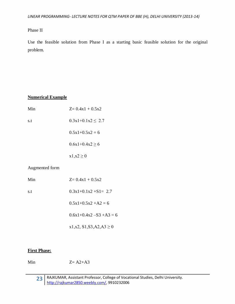
Phase II
Use the feasible solution from Phase I as a starting basic feasible solution for the original
problem.
Numerical Example
Min Z= 0.4x1 + 0.5x2
s.t 0.3x1+0.1x2 ≤ 2.7
0.5x1+0.5x2 = 6
0.6x1+0.4x2 ≥ 6
x1,x2 ≥ 0
Augmented form
Min Z= 0.4x1 + 0.5x2
s.t 0.3x1+0.1x2 +S1= 2.7
0.5x1+0.5x2 +A2 = 6
0.6x1+0.4x2 –S3 +A3 = 6
x1,x2, S1,S3,A2,A3 ≥ 0
First Phase:
Min Z= A2+A3

LINEAR PROGRAMMING- LECTURE NOTES FOR QTM PAPER OF BBE (H), DELHI UNIVERSITY (2013-14)
24 RAJKUMAR, Assistant Professor, College of Vocational Studies, Delhi University. http://rajkumar2850.weebly.com/, 9910232006
s.t 0.3x1+0.1x2 +S1= 2.7
0.5x1+0.5x2 +A2 = 6
0.6x1+0.4x2 –S3 +A3 = 6
x1,x2, S1,S3,A2,A3 ≥ 0
OR
Max -Z + A2+A3 =0
s.t 0.3x1+0.1x2 –S1= 2.7
0.5x1+0.5x2 +A2 = 6
0.6x1+0.4x2 –S3 +A3 = 6
x1,x2, S1,S3,A2,A3 ≥ 0
WE NEED TO TRANSFORM OBJECTIVE FUNCTION FOR GAUSSIAN
ELIMINATION
Iteration
0
Z x1 x2 S1 s3 A2 A3 RHS
Z -1 0 0 0 0 1 1 0
S1 0 0.3 0.1 1 0 0 0 2.7
A2 0 0.5 0.5 0 0 1 0 6
A3 0 0.6 0.4 0 -1 0 1 6
As in case of Big M method, we need to eliminate the basic variable A2 and A3 from objective
function.
LINEAR PROGRAMMING- LECTURE NOTES FOR QTM PAPER OF BBE (H), DELHI UNIVERSITY (2013-14)
25 RAJKUMAR, Assistant Professor, College of Vocational Studies, Delhi University. http://rajkumar2850.weebly.com/, 9910232006
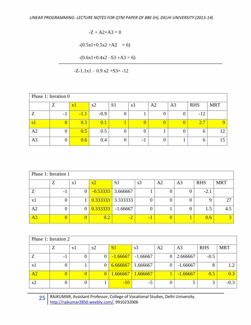
-Z + A2+A3 = 0
-(0.5x1+0.5x2 +A2 = 6)
-(0.6x1+0.4x2 –S3 +A3 = 6)
-Z-1.1x1 – 0.9 x2 +S3= -12
Phase 1: Iteration 0
Z x1 x2 S1 s3 A2 A3 RHS MRT
Z -1 -1.1 -0.9 0 1 0 0 -12
s1 0 0.3 0.1 1 0 0 0 2.7 9
A2 0 0.5 0.5 0 0 1 0 6 12
A3 0 0.6 0.4 0 -1 0 1 6 15
Phase 1: Iteration 1
Z x1 x2 S1 s3 A2 A3 RHS MRT
Z -1 0 -0.53333 3.666667 1 0 0 -2.1
x1 0 1 0.333333 3.333333 0 0 0 9 27
A2 0 0 0.333333 -1.66667 0 1 0 1.5 4.5
A3 0 0 0.2 -2 -1 0 1 0.6 3
Phase 1: Iteration 2
Z x1 x2 S1 s3 A2 A3 RHS MRT
Z -1 0 0 -1.66667 -1.66667 0 2.666667 -0.5
x1 0 1 0 6.666667 1.666667 0 -1.66667 8 1.2
A2 0 0 0 1.666667 1.666667 1 -1.66667 0.5 0.3
x2 0 0 1 -10 -5 0 5 3 -0.3
LINEAR PROGRAMMING- LECTURE NOTES FOR QTM PAPER OF BBE (H), DELHI UNIVERSITY (2013-14)
26 RAJKUMAR, Assistant Professor, College of Vocational Studies, Delhi University. http://rajkumar2850.weebly.com/, 9910232006
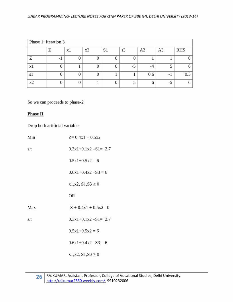
Phase 1: Iteration 3
Z x1 x2 S1 s3 A2 A3 RHS
Z -1 0 0 0 0 1 1 0
x1 0 1 0 0 -5 -4 5 6
s1 0 0 0 1 1 0.6 -1 0.3
x2 0 0 1 0 5 6 -5 6
So we can proceeds to phase-2
Phase II
Drop both artificial variables
Min Z= 0.4x1 + 0.5x2
s.t 0.3x1+0.1x2 –S1= 2.7
0.5x1+0.5x2 = 6
0.6x1+0.4x2 –S3 = 6
x1,x2, S1,S3 ≥ 0
OR
Max -Z + 0.4x1 + 0.5x2 =0
s.t 0.3x1+0.1x2 –S1= 2.7
0.5x1+0.5x2 = 6
0.6x1+0.4x2 –S3 = 6
x1,x2, S1,S3 ≥ 0

LINEAR PROGRAMMING- LECTURE NOTES FOR QTM PAPER OF BBE (H), DELHI UNIVERSITY (2013-14)
27 RAJKUMAR, Assistant Professor, College of Vocational Studies, Delhi University. http://rajkumar2850.weebly.com/, 9910232006
Use the initial basic variable from last iteration level of phase I
Phase 2: Iteration 0
Z x1 x2 S1 s3 RHS
Z -1 0.4 0.5 0 0 0
x1 0 1 0 0 -5 6
s1 0 0 0 1 1 0.3
x2 0 0 1 0 5 6
Again we need to eliminate the basic variable from objective function i.e. the coefficient of basic
variable must be zero in objective function. So we will do following
Z row – 0.4 (x1 row) – 0.5 (x2 row)
Therefore the coefficient of z row become
( -1 0 0 0 -0.5 -5.4)
Phase 2: Iteration 0
Z x1 x2 S1 s3 RHS MRT
Z -1 0 0 0 -0.5 -5.4
x1 0 1 0 0 -5 6 -1.2
s1 0 0 0 1 1 0.3 0.3
x2 0 0 1 0 5 6 1.2
Phase 2: Iteration 1 Optimal Solution
Z x1 x2 S1 s3 RHS
Z -1 0 0 0.5 0 -5.25
x1 0 1 0 5 0 7.5

LINEAR PROGRAMMING- LECTURE NOTES FOR QTM PAPER OF BBE (H), DELHI UNIVERSITY (2013-14)
28 RAJKUMAR, Assistant Professor, College of Vocational Studies, Delhi University. http://rajkumar2850.weebly.com/, 9910232006
S3 0 0 0 1 1 0.3
x2 0 0 1 -5 0 4.5
Solution from Big M and Two phase method is same. The Two phase method is considered as
improvement over Big M Methods but essentially both methods are same. The comparsion of
both method is given in next section.
Big M v/s Two Phase method
Suppose that our problem is following
Z= c1X1 + c2X2
Subject to
a11X1 +a12X2 ≥ b1
a21X2 + a22X2 ≥ b2
Xi ≥ 0
The objective function in both methods will be following
LINEAR PROGRAMMING- LECTURE NOTES FOR QTM PAPER OF BBE (H), DELHI UNIVERSITY (2013-14)
29 RAJKUMAR, Assistant Professor, College of Vocational Studies, Delhi University. http://rajkumar2850.weebly.com/, 9910232006
Big M method-
Z= c1X1 + c2X2 + MA1 + MA2
Two phase method
Phase I: Z= A1 + A2
Phase II: Z= c1X1 + c2X2
Because the MA1 and MA2 terms dominate the c1X1 and c2X2 terms in the objective function for
the Big M method, this objective function is essentially equivalent to the phase I objective
function as long as A1 and or A2 is greater than zero. Then, when both A1= 0 and A2=0, the
objective function for the Big M method becomes completly equivalent to the phase II objective
function.
Because of these virtual equivalencies in objective functions, the Big M and two phase methods
generally have the same sequence of BF solutions. The one possible exception occurs when there
is a tie for the entering basic variable in phase I of the two phase method.
The two phase method streamlines the Big M method by using only the multiplicative factors in
phase I and by dropping the artificial variables in phase II. For these reasons, the two phase
method is commonly used in computer codes.
LINEAR PROGRAMMING- LECTURE NOTES FOR QTM PAPER OF BBE (H), DELHI UNIVERSITY (2013-14)
30 RAJKUMAR, Assistant Professor, College of Vocational Studies, Delhi University. http://rajkumar2850.weebly.com/, 9910232006
Duality
The term ‘dual’ in general sense implies two or double. In the context of LP, duality implies that
each linear programming can be analysed in two different ways but having equivalent solutions.
Each LP problem (both maximization and minimization) stated in its original form has
associated with another LP problem (called dual LP), which is unique and based on the same
data.
The dual and primal LP are so closely related that the optimal solution of one problem
automatically provides the optimal solution to the others.
To show how the dual problem is constructed, defined the primal in equation form as follows
Max Z= c1x1 + c2x2
s.t. a11x1 + a12x2 +S1 = b1
a21x1 + a22x2 + S2= b2
x1, x2 ≥ 0
(Note- it is augmented form, You may also have surplus variables, if any)
Rules for Duality
1. A dual variable is defined for each primal (constraint) equation.
2. A dual constraint is defined for each primal variable.
3. The constraint (column) coefficient of a primal variable define the left hand side
coefficients of the dual constraint and its objective coefficient define the RHS.
4. The objective coefficients of the dual equal the RHS of the primal constraint equations.
LINEAR PROGRAMMING- LECTURE NOTES FOR QTM PAPER OF BBE (H), DELHI UNIVERSITY (2013-14)
31 RAJKUMAR, Assistant Professor, College of Vocational Studies, Delhi University. http://rajkumar2850.weebly.com/, 9910232006
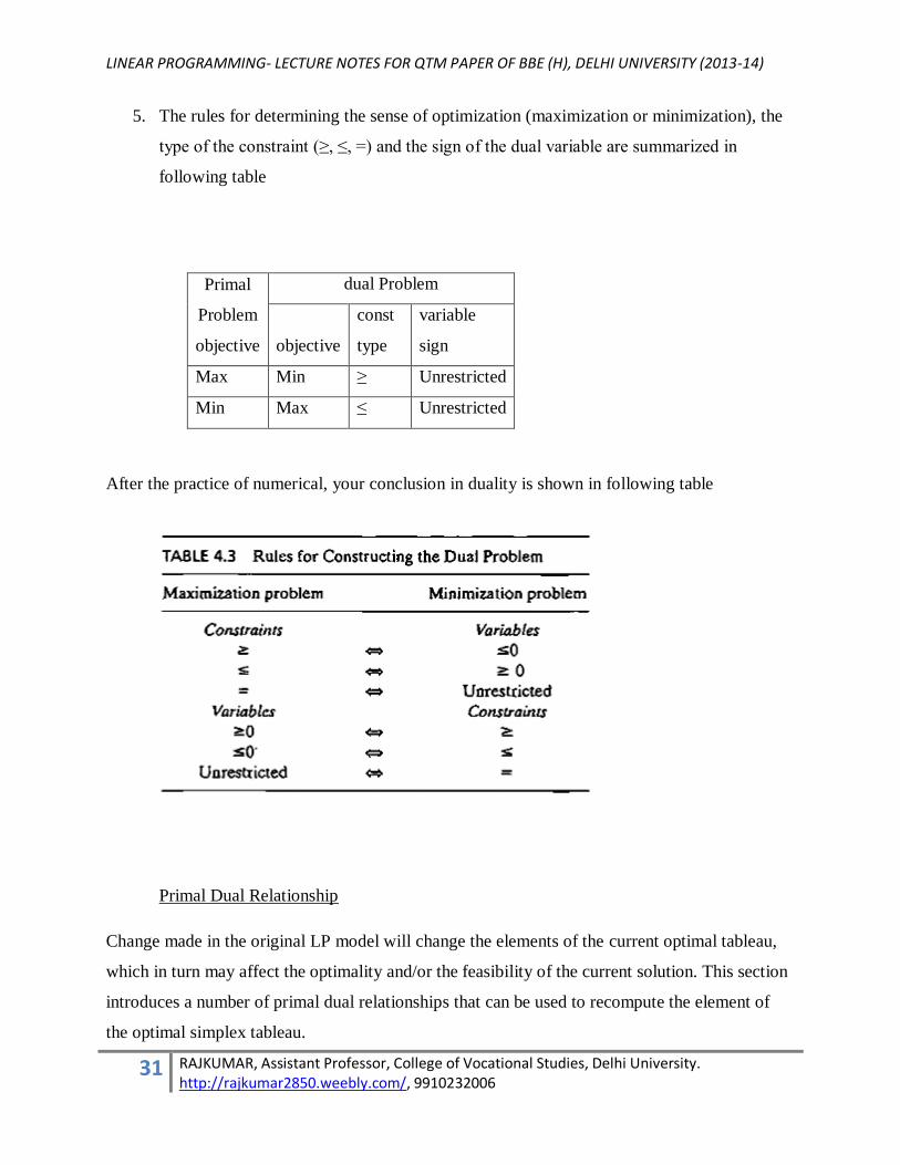
5. The rules for determining the sense of optimization (maximization or minimization), the
type of the constraint (≥, ≤, =) and the sign of the dual variable are summarized in
following table
Primal
Problem
objective
dual Problem
objective
const
type
variable
sign
Max Min ≥ Unrestricted
Min Max ≤ Unrestricted
After the practice of numerical, your conclusion in duality is shown in following table
Primal Dual Relationship
Change made in the original LP model will change the elements of the current optimal tableau,
which in turn may affect the optimality and/or the feasibility of the current solution. This section
introduces a number of primal dual relationships that can be used to recompute the element of
the optimal simplex tableau.

LINEAR PROGRAMMING- LECTURE NOTES FOR QTM PAPER OF BBE (H), DELHI UNIVERSITY (2013-14)
32 RAJKUMAR, Assistant Professor, College of Vocational Studies, Delhi University. http://rajkumar2850.weebly.com/, 9910232006
1. Optimal dual solution- the primal and dual solution are so closely related that the optimal
solution of either problem directly yield (with little additional computation) the optimal
solution to the other
Optimal value of dual variable Yi = (optimal primal coefficient of initial basic variables,
xi + (Original objective coefficient of xi)
Example
Primal LP
Max Z= 5x1 + 12x2
X1 + 2x2 + x3 ≤ 10
2x1 – x2 + 3x3 = 8
x1, x2, x3 ≥ 0
its augmented form
Max Z= 5x1 + 12x2
X1 + 2x2 + x3 +s1 = 10
2x1 – x2 + 3x3 = 8
x1, x2, x3 ≥ 0
so dual LP
Min Z’= 10y1 + 8y2
y1 + 2y2 ≥ 5
2y1 – y2 ≥ 12
y1 + 3y2 ≥ 4
y1 ≥ 0 and y2 unrestricted

LINEAR PROGRAMMING- LECTURE NOTES FOR QTM PAPER OF BBE (H), DELHI UNIVERSITY (2013-14)
33 RAJKUMAR, Assistant Professor, College of Vocational Studies, Delhi University. http://rajkumar2850.weebly.com/, 9910232006
The optimal solution of primal LP is given in following table
Basic
Variable
coefficient of
RHS x1 x2 x3 S1 A2
Z 0 0 3/2 29/5 -2/5 + M 216/5
x2 0 1 -1/5 2/5 -1/5 12/5
x1 1 0 7/5 1/5 2/5 26/5
From the optimal solution of primal LP, we can directly derive the solution of its dual LP. It is
shown in following table
Starting Primal Basic
Variable S1 R
Z equation coefficient 29/5 -2/5 + M
Original objective
coefficient 0 -M
Dual variable y1 y2
Optimal dual variable
29/5 +
0 =29/5
-2/5 + M – M= -
2/5
2. In any simplex iteration, the objective equation coefficient of xj is computed as follows
Primal z equation coefficient of variable xj= (LHS of jth dual constraint) – (RHS of jth dual
constraint)
In the previous example,

LINEAR PROGRAMMING- LECTURE NOTES FOR QTM PAPER OF BBE (H), DELHI UNIVERSITY (2013-14)
34 RAJKUMAR, Assistant Professor, College of Vocational Studies, Delhi University. http://rajkumar2850.weebly.com/, 9910232006
This relationship is very useful for transportation problem, the MODI method uses this
relationship to test optimality in transportation problem.
3. For any pair of feasible primal and dual solutions,
At the optimum, the relationship holds with equality. The relationship does not specifiy which
problem is primal and which is dual.
Duality Theorem
Optimum
Max Z Min Z’
Objective values
in the Maxi
problem
Objective
values in the
Mini problem

LINEAR PROGRAMMING- LECTURE NOTES FOR QTM PAPER OF BBE (H), DELHI UNIVERSITY (2013-14)
35 RAJKUMAR, Assistant Professor, College of Vocational Studies, Delhi University. http://rajkumar2850.weebly.com/, 9910232006
The following are the only possible relationship between the primal and dual problem
1. If one problem has feasible solutions, and a bounded objective function (and so has an
optimal solution) then so does the other problem, so both weak and strong duality
properties are applicable.
2. If one problem has feasible solutions and an unbounded objective function (and no
optimal solution) then the other problem has no feasible solutions
3. If one problem has no feasible solutions, then the other problem has either no feasible
solutions or an unbounded objective function.
Advantages of duality
Duality is an extremely important and interesting feature of linear programming. The various
useful aspects of this property are
1. If the primal problem contains a large number of rows (constraints) and a smaller number
of columns (variables), the computational procedure can be considerably reduced by
converting it into dual and then solving it. Hence it offers an advantage in many
applications.
2. It gives additional information as to how the optimal solution changes as a result of the
changes in the coefficients and the formulation of the problem. This forms the basis of
post optimality or sensitivity analysis.
3. Duality in linear programming has certain far reaching consequences of economic nature.
This can help managers answer questions about alternative courses of action and their
relative values.
4. Calculation of the dual checks the accuracy of the primal solution.
5. Duality in linear programming shows that each linear programme is equivalent to a two-
person zero-sum game for player A and player B. This indicates that fairly close
relationships exist between linear programming and the theory of games.
6. Duality is not restricted to linear programming problems only but finds application in
economics, management and other fields. In economics it is used in the formulation of
input and output systems.
7. Economic interpretation ofthe dual helps the management in making future decisions.

LINEAR PROGRAMMING- LECTURE NOTES FOR QTM PAPER OF BBE (H), DELHI UNIVERSITY (2013-14)
36 RAJKUMAR, Assistant Professor, College of Vocational Studies, Delhi University. http://rajkumar2850.weebly.com/, 9910232006
8. Duality is used to solve L.P. problems (by the dual simplex method) in which the initial
solution is infeasible.