linear programming mcgraw-hill/irwin copyright © 2012 by the mcgraw-hill companies, inc. all rights...
TRANSCRIPT
Linear Programming
Chapter 19
McGraw-Hill/Irwin Copyright © 2012 by The McGraw-Hill Companies, Inc. All rights reserved.

Chapter 19: Learning Objectives
You should be able to:1. Describe the type of problem that would lend itself to
solution using linear programming2. Formulate a linear programming model from a
description of a problem3. Solve simple linear programming problems using the
graphical method4. Interpret computer solutions of linear programming
problems5. Do sensitivity analysis on the solution of a linear
programming problem
Instructor Slides 19-2
Linear Programming (LP)LP
A powerful quantitative tool used by operations and other manages to obtain optimal solutions to problems that involve restrictions or limitationsApplications include:
Establishing locations for emergency equipment and personnel to minimize response time
Developing optimal production schedulesDeveloping financial plansDetermining optimal diet plans
Instructor Slides 19-3
LP ModelsLP Models
Mathematical representations of constrained optimization problems
LP Model Components:Objective function
A mathematical statement of profit (or cost, etc.) for a given solution
Decision variablesAmounts of either inputs or outputs
ConstraintsLimitations that restrict the available alternatives
ParametersNumerical constants
Instructor Slides 19-4
6S-5
Used to obtain optimal solutions to problems that involve restrictions or limitations, such as:MaterialsBudgetsLaborMachine time
Linear programming (LP) techniques consist of a sequence of steps that will lead to an optimal solution to problems, in cases where an optimum exists
Linear Programming
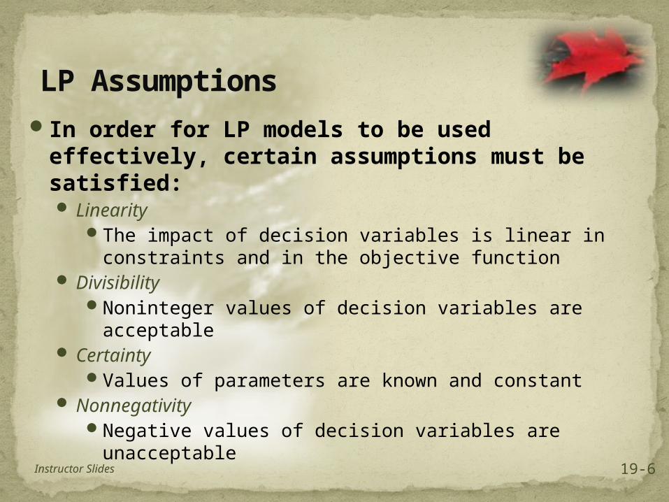
LP AssumptionsIn order for LP models to be used
effectively, certain assumptions must be satisfied: Linearity
The impact of decision variables is linear in constraints and in the objective function
DivisibilityNoninteger values of decision variables are
acceptable Certainty
Values of parameters are known and constant Nonnegativity
Negative values of decision variables are unacceptable
Instructor Slides 19-6
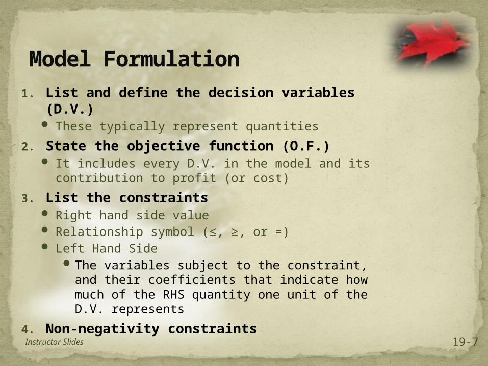
Model Formulation1. List and define the decision variables (D.V.)
These typically represent quantities
2. State the objective function (O.F.) It includes every D.V. in the model and its
contribution to profit (or cost)
3. List the constraints Right hand side value Relationship symbol (≤, ≥, or =) Left Hand Side
The variables subject to the constraint, and their coefficients that indicate how much of the RHS quantity one unit of the D.V. represents
4. Non-negativity constraints
Instructor Slides 19-7
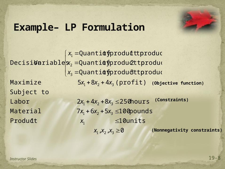
Example– LP Formulation
0,,
units 10 1Product
pounds 100567 Material
hours 250842 Labor
Subject to
(profit) 485 Maximize
produce to3product ofQuantity
produce to2product ofQuantity
produce to1product ofQuantity
VariablesDecision
321
1
321
321
321
3
2
1
xxx
x
xxx
xxx
xxx
x
x
x
(Objective function)
(Constraints)
(Nonnegativity constraints)
Instructor Slides 19-8

Graphical LPGraphical LP
A method for finding optimal solutions to two-variable problems
Procedure1. Set up the objective function and the constraints in
mathematical format2. Plot the constraints3. Indentify the feasible solution space
The set of all feasible combinations of decision variables as defined by the constraints
4. Plot the objective function5. Determine the optimal solution
Instructor Slides 19-9

6S-10
Linear Programming Example
Assembly Time/Unit
Inspection Time/Unit
Storage Space/Unit Profit/Unit
Model A 4 2 3 60$
Model B 10 1 3 50$
Available 100 hours 22 hours 39 cubic feet
6S-11
Linear Programming Example
Find the quantity of each model to produce in order to maximize the profit

6S-12
LP Example – Decision Variables
Decision Variables
A: # of model A product to be built
B: # of model B product to be built

Example– Graphical LP: Step 1
0,
feet cubic 3933 Storage
hours 2212 Inspection
hours 100104 Assembly
Subject to
5060 Maximize
produce to2 typeofquantity
produce to1 typeofquantity VariablesDecision
21
21
21
21
21
2
1
xx
xx
xx
xx
xx
x
x
Instructor Slides 19-13
6S-14
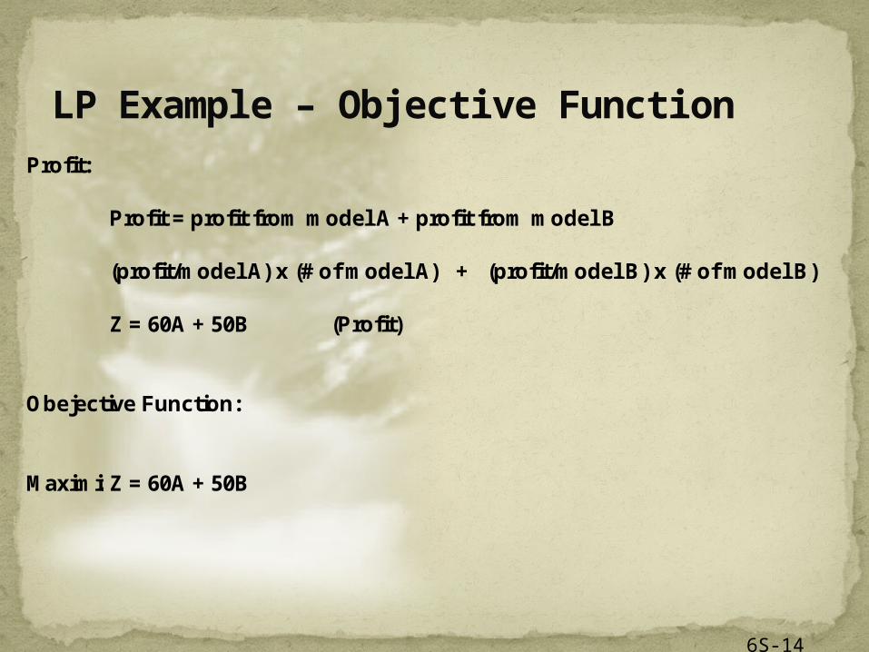
LP Example – Objective FunctionProfit:
Profit = profit from model A + profit from model B
(profit/model A) x (# of model A) + (profit/model B) x (# of model B)
Z = 60A + 50B (Profit)
Obejective Function:
MaximizeZ = 60A + 50B
6S-15
LP Example – Objective Function
0
5
10
15
20
25
30
1 2 3 4 5 6 7 8 9 10 11
A
B60A+50B=600
60A+50B=1200

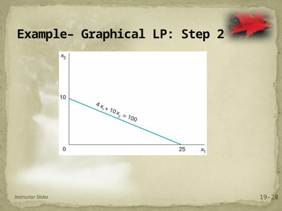
Example– Graphical LP: Step 2Plotting constraints:
Begin by placing the nonnegativity constraints on a graph
Instructor Slides 19-16
Example– Graphical LP: Step 2Plotting constraints:
1. Replace the inequality sign with an equal sign.2. Determine where the line intersects each axis3. Mark these intersection on the axes, and connect
them with a straight line4. Indicate by shading, whether the inequality is
greater than or less than5. Repeat steps 1 – 4 for each constraint
Instructor Slides 19-17
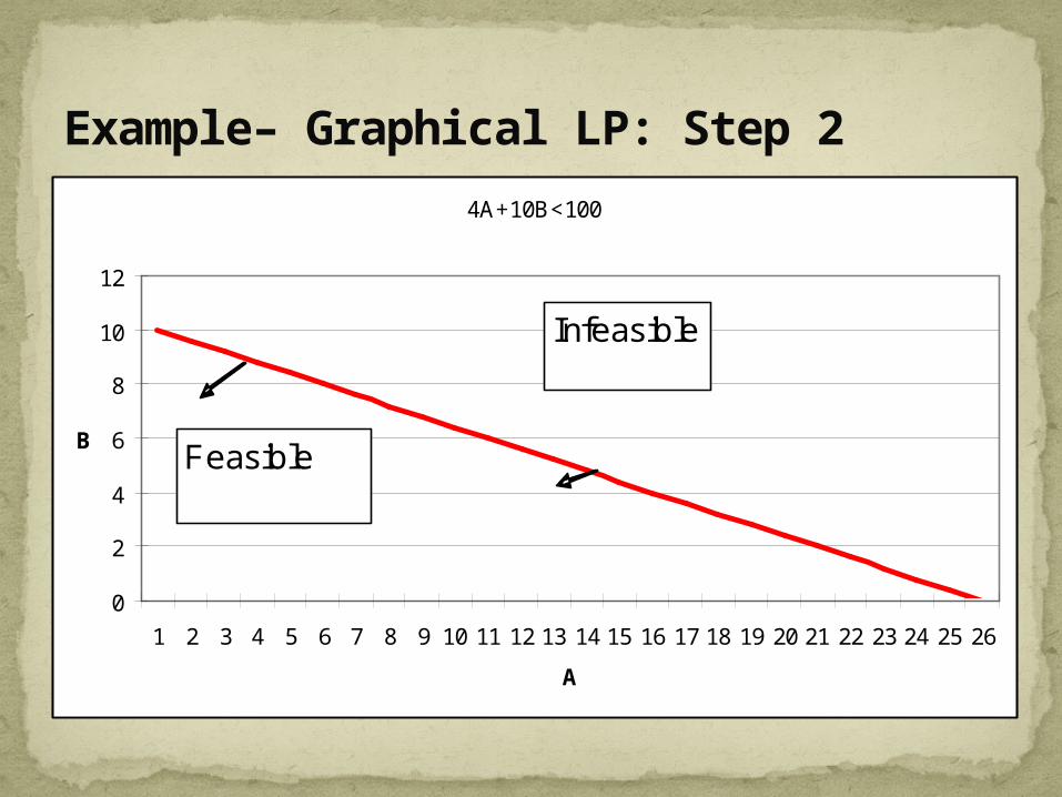
Example– Graphical LP: Step 24A+10B<100
0
2
4
6
8
10
12
1 2 3 4 5 6 7 8 9 10 11 12 13 14 15 16 17 18 19 20 21 22 23 24 25 26
A
B Feasible
Infeasible

Example– Graphical LP: Step 2
Example– Graphical LP: Step 2
Instructor Slides 19-20

Example– Graphical LP: Step 2
Instructor Slides 19-21

Example– Graphical LP: Step 2
Instructor Slides 19-22
6S-23
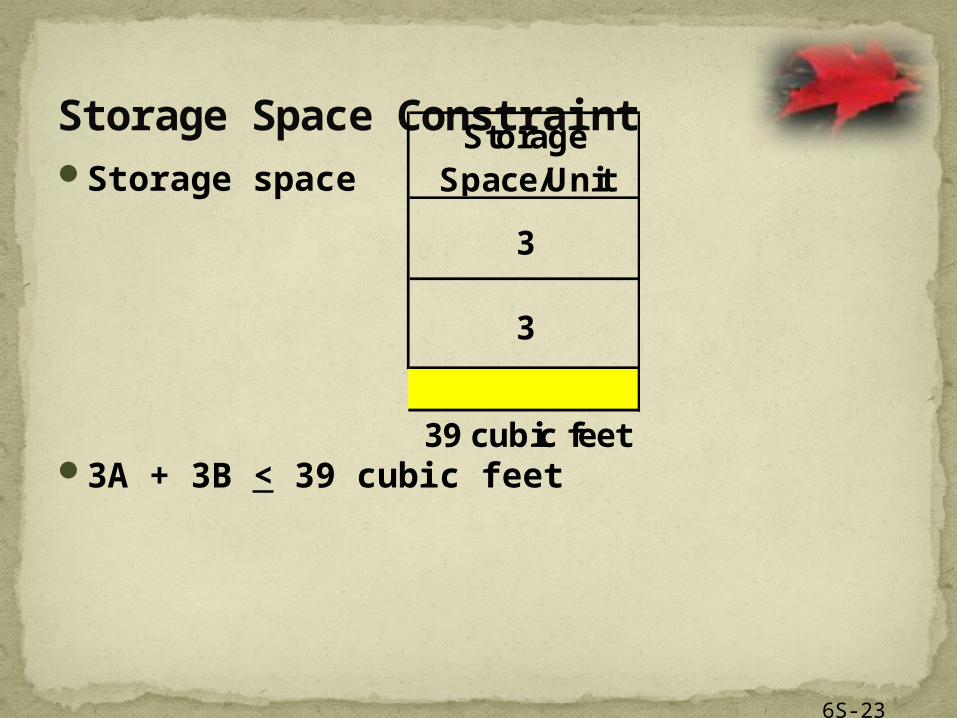
Storage Space ConstraintStorage space
3A + 3B < 39 cubic feet
Storage Space/Unit
3
3
39 cubic feet
6S-24
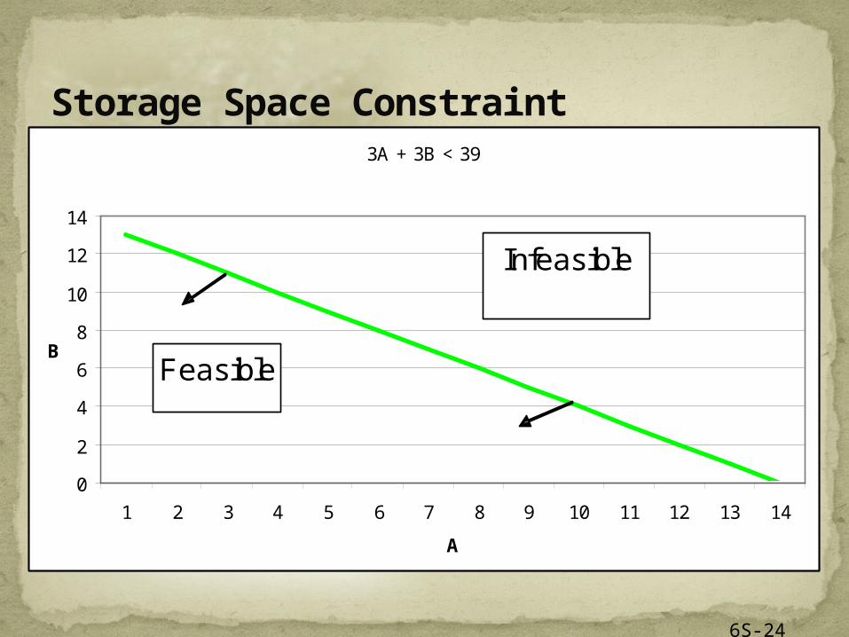
Storage Space Constraint3A + 3B < 39
0
2
4
6
8
10
12
14
1 2 3 4 5 6 7 8 9 10 11 12 13 14
A
BFeasible
Infeasible
6S-25
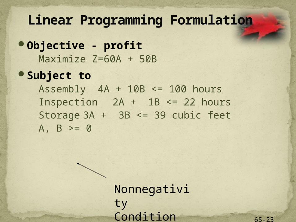
Objective - profitMaximize Z=60A + 50B
Subject toAssembly 4A + 10B <= 100 hoursInspection 2A + 1B <= 22 hoursStorage 3A + 3B <= 39 cubic feetA, B >= 0
Linear Programming Formulation
Nonnegativity Condition

Example– Graphical LP: Step 2
Instructor Slides 19-26

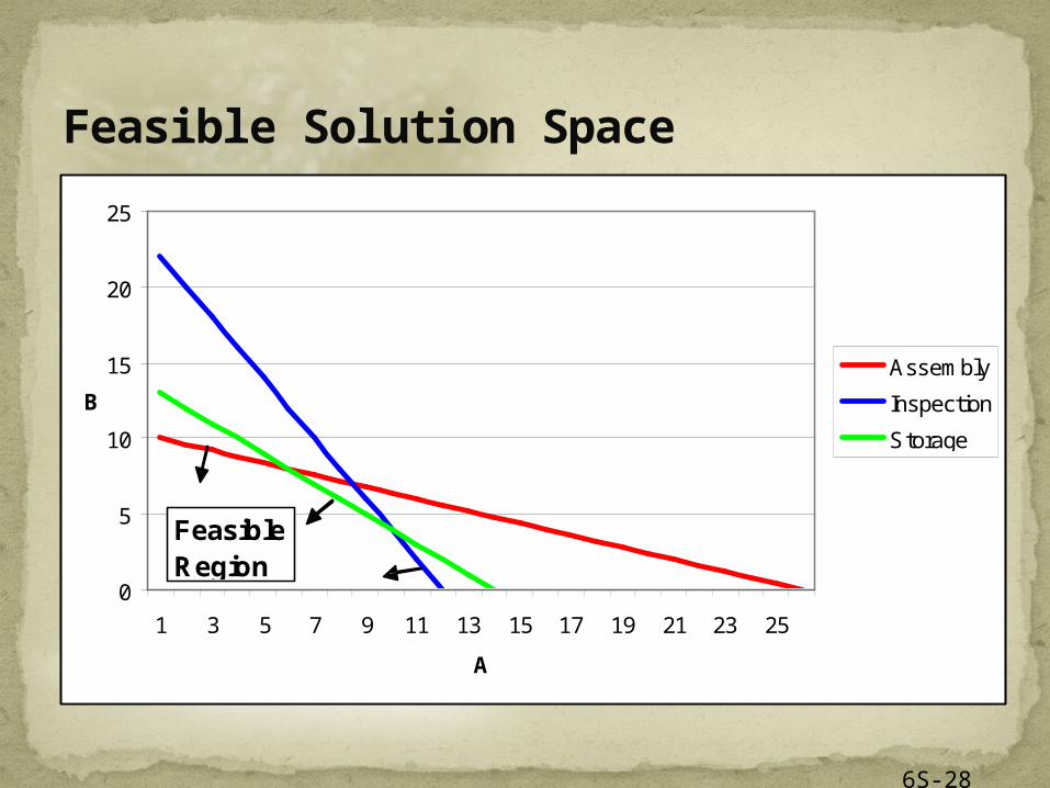
Example– Graphical LP: Step 3Feasible Solution Space
The set of points that satisfy all constraints simultaneously
Instructor Slides 19-27
6S-28
Feasible Solution Space
0
5
10
15
20
25
1 3 5 7 9 11 13 15 17 19 21 23 25
A
B
Assembly
Inspection
Storage
Feasible Region
Example– Graphical LP: Step 4Plotting the objective function line
This follows the same logic as plotting a constraint line There is no equal sign, so we simply set the objective
function to some quantity (profit or cost) The profit line can now be interpreted as an isoprofit
lineEvery point on this line represents a combination of
the decision variables that result in the same profit (in this case, to the profit you selected)
Instructor Slides 19-29
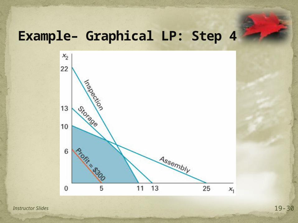
Example– Graphical LP: Step 4
Instructor Slides 19-30

6S-31
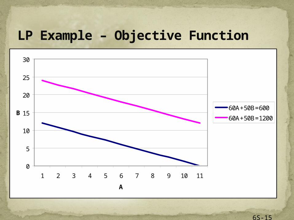
LP Example – Objective Function
0
5
10
15
20
25
30
1 2 3 4 5 6 7 8 9 10 11
A
B60A+50B=600
60A+50B=1200
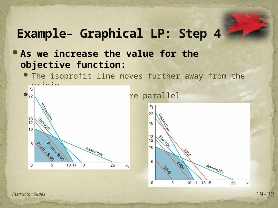
Example– Graphical LP: Step 4As we increase the value for the objective
function: The isoprofit line moves further away from the origin The isoprofit lines are parallel
Instructor Slides 19-32

Example– Graphical LP: Step 5 Where is the optimal solution?
The optimal solution occurs at the furthest point (for a maximization problem) from the origin the isoprofit can be moved and still be touching the feasible solution space
This optimum point will occur at the intersection of two constraints:
Solve for the values of x1 and x2 where this occurs
Instructor Slides 19-33

Redundant ConstraintsRedundant constraints
A constraint that does not form a unique boundary of the feasible solution space
Test:A constraint is redundant if its removal does not
alter the feasible solution space
Instructor Slides 19-34
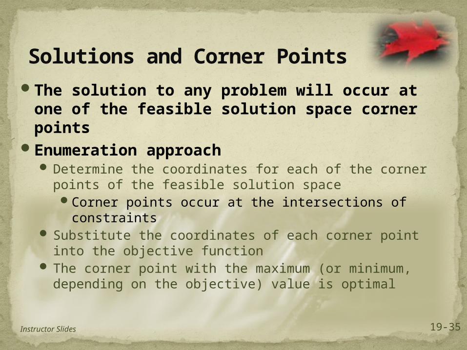
Solutions and Corner PointsThe solution to any problem will occur at one
of the feasible solution space corner pointsEnumeration approach
Determine the coordinates for each of the corner points of the feasible solution spaceCorner points occur at the intersections of
constraints Substitute the coordinates of each corner point into the
objective function The corner point with the maximum (or minimum,
depending on the objective) value is optimal
Instructor Slides 19-35

6S-36
The intersection of inspection and storage
Solve two equations with two unknowns 2A + 1B = 22
3A + 3B = 39
A = 9B = 4Z = $740
Optimal Solution
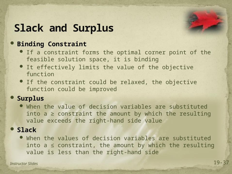
Slack and Surplus Binding Constraint
If a constraint forms the optimal corner point of the feasible solution space, it is binding
It effectively limits the value of the objective function If the constraint could be relaxed, the objective function could
be improved Surplus
When the value of decision variables are substituted into a ≥ constraint the amount by which the resulting value exceeds the right-hand side value
Slack When the values of decision variables are substituted into a ≤
constraint, the amount by which the resulting value is less than the right-hand side
Instructor Slides 19-37
6S-38
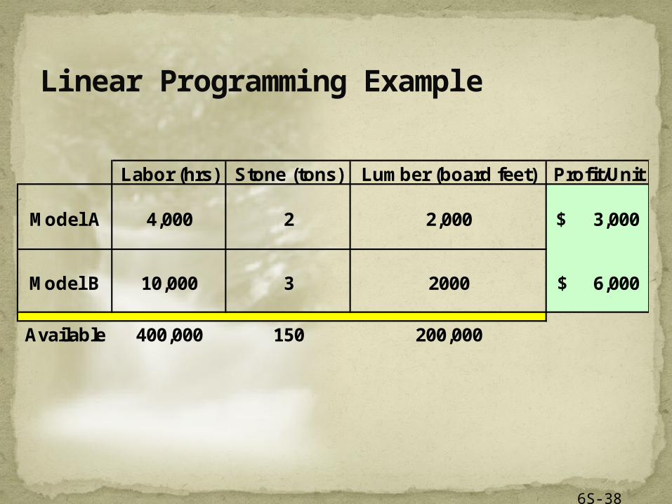
Linear Programming Example
Labor (hrs) Stone (tons) Lumber (board feet) Profit/Unit
Model A 4,000 2 2,000 3,000$
Model B 10,000 3 2000 6,000$
Available 400,000 150 200,000

The Simplex MethodSimplex method
A general purpose linear programming algorithm that can be used to solve problems having more than two decision variables
Instructor Slides 19-39

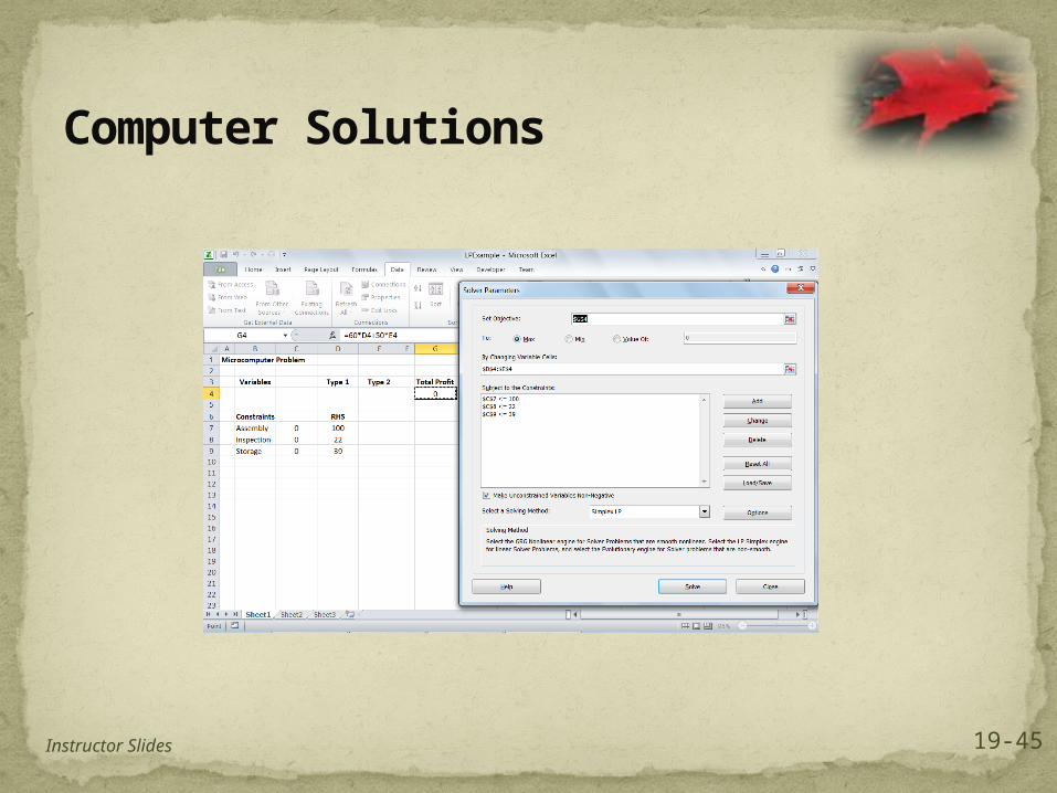
Computer SolutionsMS Excel can be used to solve LP
problems using its Solver routineEnter the problem into a worksheetWhere there is a zero in Figure 19.15, a
formula was enteredSolver automatically places a value of zero after
you input the formulaYou must designate the cells where you want
the optimal values for the decision variables
Instructor Slides 19-40
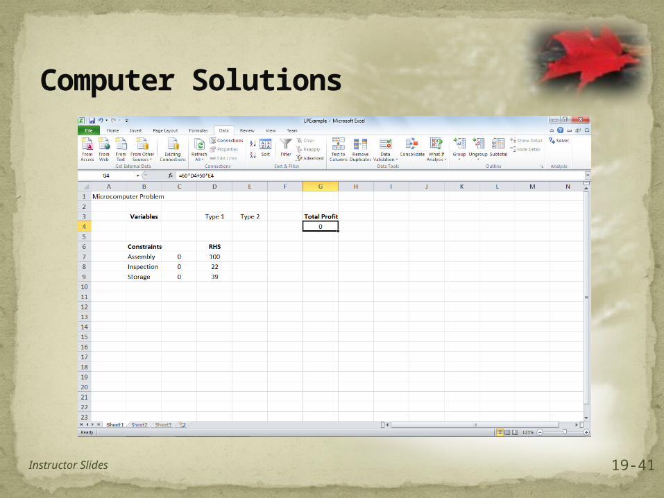
Computer Solutions
Instructor Slides 19-41
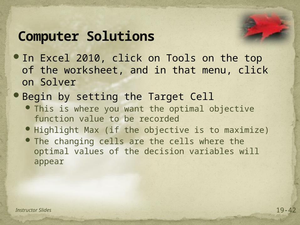
Computer SolutionsIn Excel 2010, click on Tools on the top of the
worksheet, and in that menu, click on SolverBegin by setting the Target Cell
This is where you want the optimal objective function value to be recorded
Highlight Max (if the objective is to maximize) The changing cells are the cells where the optimal
values of the decision variables will appear
Instructor Slides 19-42
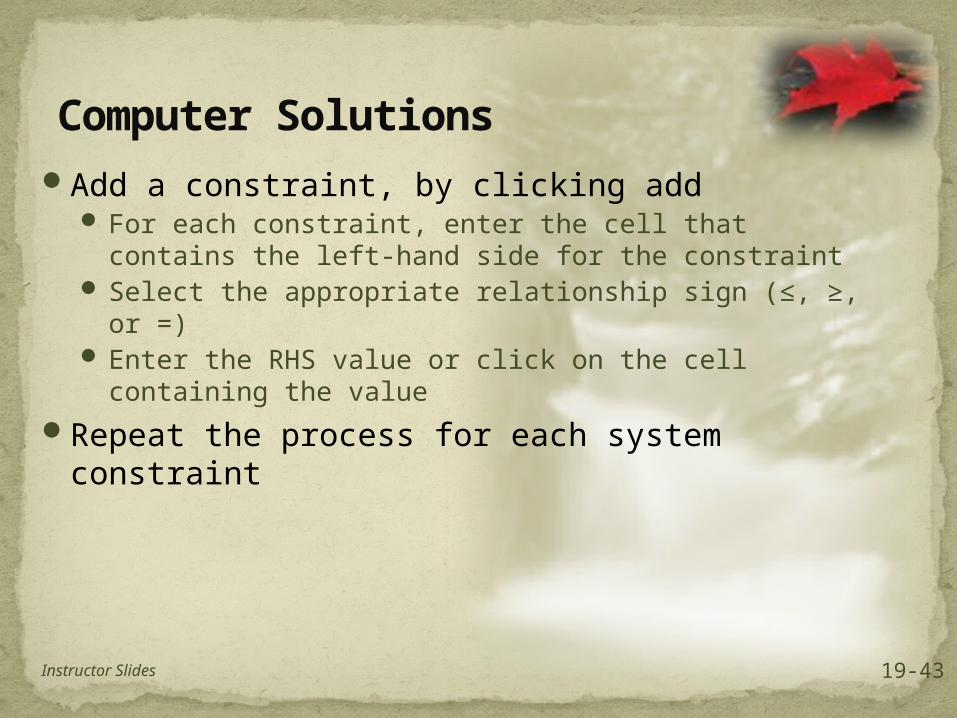
Computer SolutionsAdd a constraint, by clicking add
For each constraint, enter the cell that contains the left-hand side for the constraint
Select the appropriate relationship sign (≤, ≥, or =) Enter the RHS value or click on the cell containing the
value
Repeat the process for each system constraint
Instructor Slides 19-43
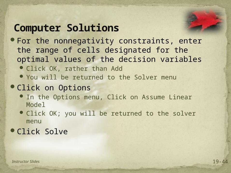
Computer SolutionsFor the nonnegativity constraints, enter the
range of cells designated for the optimal values of the decision variables Click OK, rather than Add You will be returned to the Solver menu
Click on Options In the Options menu, Click on Assume Linear Model Click OK; you will be returned to the solver menu
Click Solve
Instructor Slides 19-44
Computer Solutions
Instructor Slides 19-45

The Solver Results menu will appearYou will have one of two results
A SolutionIn the Solver Results menu Reports box
Highlight both Answer and Sensitivity Click OK
An Error messageMake corrections and click solve
Solver Results
Instructor Slides 19-46

Solver Results Solver will incorporate the optimal values of the decision
variables and the objective function into your original layout on your worksheets
Instructor Slides 19-47

Answer Report
Instructor Slides 19-48

Sensitivity Report
Instructor Slides 19-49
Sensitivity AnalysisSensitivity Analysis
Assessing the impact of potential changes to the numerical values of an LP model
Three types of changesObjective function coefficientsRight-hand values of constraintsConstraint coefficients
We will consider these
Instructor Slides 19-50
A change in the value of an O.F. coefficient can cause a change in the optimal solution of a problem
Not every change will result in a changed solution
Range of OptimalityThe range of O.F. coefficient values for which the
optimal values of the decision variables will not change
O.F. Coefficient Changes
Instructor Slides 19-51

Basic and Non-Basic VariablesBasic variables
Decision variables whose optimal values are non-zero
Non-basic variablesDecision variables whose optimal values are
zeroReduced cost
Unless the non-basic variable’s coefficient increases by more than its reduced cost, it will continue to be non-basic
Instructor Slides 19-52

RHS Value ChangesShadow price
Amount by which the value of the objective function would change with a one-unit change in the RHS value of a constraint
Range of feasibilityRange of values for the RHS of a constraint over
which the shadow price remains the same
Instructor Slides 19-53

Binding vs. Non-binding ConstraintsNon-binding constraints
have shadow price values that are equal to zero have slack (≤ constraint) or surplus (≥ constraint) Changing the RHS value of a non-binding constraint (over its
range of feasibility) will have no effect on the optimal solutionBinding constraint
have shadow price values that are non-zero have no slack (≤ constraint) or surplus (≥ constraint) Changing the RHS value of a binding constraint will lead to a
change in the optimal decision values and to a change in the value of the objective function
Instructor Slides 19-54