linear polygraphs and koszulity of algebras
TRANSCRIPT
HAL Id: hal-01006220https://hal.archives-ouvertes.fr/hal-01006220v1Preprint submitted on 14 Jun 2014 (v1), last revised 8 Oct 2018 (v3)
HAL is a multi-disciplinary open accessarchive for the deposit and dissemination of sci-entific research documents, whether they are pub-lished or not. The documents may come fromteaching and research institutions in France orabroad, or from public or private research centers.
L’archive ouverte pluridisciplinaire HAL, estdestinée au dépôt et à la diffusion de documentsscientifiques de niveau recherche, publiés ou non,émanant des établissements d’enseignement et derecherche français ou étrangers, des laboratoirespublics ou privés.
Linear polygraphs and Koszulity of algebrasYves Guiraud, Eric Hoffbeck, Philippe Malbos
To cite this version:Yves Guiraud, Eric Hoffbeck, Philippe Malbos. Linear polygraphs and Koszulity of algebras. 2014.�hal-01006220v1�
LINEAR POLYGRAPHS AND KOSZULITY OF ALGEBRAS
YVES GUIRAUD ERIC HOFFBECK PHILIPPE MALBOS
Abstract – We define higher dimensional linear rewriting systems, called linear polygraphs, for
presentations of associative algebras, generalizing the notion of noncommutative Gröbner bases.
They are constructed on the notion of category enriched in higher-dimensional vector spaces. Linear
polygraphs allow more possibilities of termination orders than those associated to Gröbner bases. We
introduce polygraphic resolutions of algebras giving a description obtained by rewriting of higher-
dimensional syzygies for presentations of algebras. We show how to compute polygraphic resolu-
tions starting from a convergent presentation, and how to relate these resolutions with the Koszul
property of algebras.
M.S.C. 2010 – 18C10, 18D05, 18G10, 16S37, 68Q42.
1 Introduction 2
2 Linear polygraphs 5
2.1 Higher-dimensional vector spaces . . . . . . . . . . . . . . . . . . . . . . . . . . . 5
2.2 Higher-dimensional algebroids . . . . . . . . . . . . . . . . . . . . . . . . . . . . . 9
2.3 Graded linear polygraphs . . . . . . . . . . . . . . . . . . . . . . . . . . . . . . . . 11
3 Two-dimensional linear rewriting systems 13
3.1 Linear 2-polygraph . . . . . . . . . . . . . . . . . . . . . . . . . . . . . . . . . . . 13
3.2 Rewriting properties of linear 2-polygraphs . . . . . . . . . . . . . . . . . . . . . . 14
3.3 The basis of irreducibles . . . . . . . . . . . . . . . . . . . . . . . . . . . . . . . . 18
3.4 Associative Gröbner bases . . . . . . . . . . . . . . . . . . . . . . . . . . . . . . . 20
4 Polygraphic resolutions of algebroids 22
4.1 Polygraphic resolutions of algebroids and normalisation strategies . . . . . . . . . . 22
4.2 Polygraphic resolutions from convergence . . . . . . . . . . . . . . . . . . . . . . . 25
5 Free resolutions of algebroids 30
5.1 Free modules resolution from polygraphic resolutions . . . . . . . . . . . . . . . . . 30
5.2 Finiteness properties . . . . . . . . . . . . . . . . . . . . . . . . . . . . . . . . . . 34
5.3 Convergence and Koszulity . . . . . . . . . . . . . . . . . . . . . . . . . . . . . . . 35
June 14, 2014
1. Introduction
1. INTRODUCTION
In homological algebra, several constructive methods based on noncommutative Gröbner bases were
developed to compute projective resolutions for algebras. In particular, these methods lead to relate the
Koszul property for an associative algebra to the existence of a quadratic Gröbner basis for its ideal
of relations: an associative algebra having a presentation by a quadratic Gröbner basis is Koszul. In
this article, we explain how these constructions can be interpreted from the point of view of higher-
dimensional rewriting theory. Moreover, we use this setting to develop several improvements of these
methods.
We define linear polygraphs as higher-dimensional linear rewriting systems for presentations of al-
gebras, generalizing the notion of noncommutative Gröbner bases. Linear polygraphs allow more pos-
sibilities of termination orders than those associated to Gröbner bases, only based on monomial orders.
Moreover, we introduce polygraphic resolutions of algebras giving a description obtained by rewriting
of higher-dimensional syzygies for presentations of algebras. We show how to compute polygraphic
resolutions starting from a convergent presentation, and how to relate these resolutions with the Koszul
property.
An overview on rewriting and Koszulity
Linear rewriting and Gröbner bases. In order to effectively compute normal forms in algebras, to
decide the word problem (ideal membership) or to construct bases (e.g., Poincaré-Birkhoff-Witt bases),
Buchberger and Shirshov have independently introduced the notion of Gröbner bases for commutative
and Lie algebras, respectively [13, 30]. Subsequently, Gröbner bases have been developed for other types
of algebras, such as associative algebras by Bokut [11] and by Bergman [10]. The notion of Gröbner
bases had already been introduced by Hironaka in [22], under the name of standard bases but without a
constructive method for computing such bases.
Consider an algebra A presented by a set of generators X and a set of relations R, that is A is the
quotient of the free algebra K〈X〉 by the congruence generated by R. The elements of the free monoid
X∗ form a linear basis of the free algebra K〈X〉. One main application of Gröbner bases is to explicitly
find a basis of the algebra A, in the form of a subset of X∗. This is based on a monomial order on
the monoid X∗ and the idea is to change the presentation of the ideal generated by R with respect to
this order. The property that the new presentation has to satisfy is the algebraic counterpart of the
confluence of a rewriting system. The central theorem for Gröbner basis is the counterpart of Newman’s
lemma. In particular, Buchberger’s algorithm, producing Gröbner bases, is in essence the analogue of
Knuth-Bendix’s completion procedure in a linear setting. Several frameworks unify Buchberger and
Knuth-Bendix algorithms, in particular a Gröbner basis corresponds to a convergent (i.e., confluent and
terminating) presentation of an algebra, see [14]. This correspondence is well known in the case of
associative and commutative algebras, as recalled in the papers of Bergman, Mora and Ufnarovski [10,
27, 34].
Gröbner bases and projectives resolutions. At the end of 1980s, through Anick’s and Green’s works
[1, 2, 3, 19], non-commutative Gröbner bases have found new applications for the study of algebras as a
constructive method to compute free resolutions. Their constructions provide small explicit resolutions
to compute homological invariants (homology groups, Hilbert and Poincaré series) of algebras presented
by generators and relations defined by a Gröbner basis. We refer the reader to [34] for a survey on
Anick’s resolution and to [5] for an implementation of the resolution. Nevertheless, the chains (given
by some of the iterated overlaps of the leading terms of the Gröbner basis) and the differential in these
resolutions are constructed recursively, which makes computations sometimes complicated.
2
1. Introduction
Confluence and Koszulity. Recall that a connected graded algebra is called Koszul if it has a nice
homological property, which can be defined in several equivalent ways. For instance, A is Koszul if the
Tor groups TorAk,(i)(K,K) vanish for i 6= k (where the first grading is the homological degree and the
second grading corresponds to the internal grading of the algebra). The property can be also be stated in
terms of existence of a linear minimal graded free resolution of K seen as a A-module. This notion was
generalized by Berger in [8] to the case of N-homogeneous algebras, asking that TorAk,(i)(K,K) vanish
for i 6= ℓN(k), where ℓN : N→ N is the function defined by
ℓN(k) =
{lN if k = 2l,
lN+ 1 if k = 2l+ 1,
for any integer k. In what follows, we will call Koszul algebras the generalized notion.
Anick’s resolutions can be used to prove Koszulity of an algebra. Indeed, if an algebra A has a
quadratic Gröbner basis, then Anick’s resolution is concentrated in the right bidegree, and thus A is
Koszul (see for instance Green and Huang [18, Theorem 9]). Another way to prove this result is that the
existence of a quadratic Gröbner basis implies the existence of a Poincaré-Birkhoff-Witt basis of A (see
Green [19, Proposition 2.14]). For the N-homogeneous case, a Gröbner basis concentrated in weight
N is not enough to imply Koszulity: an extra condition has to be checked as shown by Berger in [8,
Theorem 3.6]. When the algebra is monomial, this extra condition corresponds to the overlap property
defined by Berger in [8, Proposition 3.8.]. This property consists in a combinatorial condition based on
overlaps of the monomials of the relations.
Yet another method to prove Koszulity of algebras using a Gröbner basis can be found in the book
of Loday and Vallette [25, Chap. 4]. The quadratic Gröbner basis method to prove Koszulity has been
extended to the case of operads, see Dotsenko and Khoroshkin [16] or [25, Chap. 8].
All the constructions mentioned above rely on a monomial order, that is a well-founded total order
of the monomials. The termination orders in linear polygraph introduced in this work are less restrictive.
Organisation and main results of the article
The next section consists in presenting the categorical background of our constructions. In Section 3, we
develop the notion of linear rewriting system for algebras and we explain the links with Gröbner bases.
In Section 4, we give a method to construct polygraphic resolutions for an algebra from a convergent
presentation of these algebra. In the last section, we show that polygraphic resolutions induce free
modules resolutions for algebroids. We deduce finiteness conditions and several sufficient conditions for
an algebroid to be Koszul. We now give a detailed preview of the main construction and results of the
article.
Higher-dimensional algebroids. In Section 2.1, we introduce the notion of graded n-vector space as
an internal (strict globular) (n − 1)-category in the category of non-negatively graded spaces GrVect.
This definition extends in higher dimensions the notion of 2-vector space introduced by Baez and Crans
in [6]. An 1-algebroid (which we call algebroid from now on) is an algebra with several objects, also
called K-category by Mitchell in [26]. We define in Section 2.2 a graded n-algebroid as a category
enriched in graded n-vector spaces. Note that the Bourn’s equivalence, [12, Theorem 3.3], states that the
category of graded n-algebroids is equivalent to the category of graded chain complexes of length n.
Linear polygraphs. Higher-dimensional rewriting has unified several paradigms of rewriting. This ap-
proach is based on presentations by generators and relations of higher-dimensional categories, indepen-
dently introduced by Burroni and Street under the respective names of polygraphs in [15] and computads
in [32, 33]. The notion of linear polygraph extends this framework to a linear setting. A string (or path)
3
1. Introduction
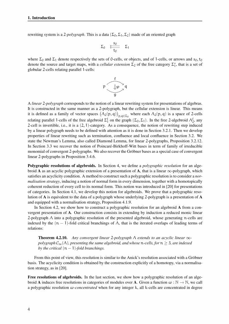
rewriting system is a 2-polygraph. This is a data (Σ0, Σ1, Σ2) made of an oriented graph
Σ0 Σ1t0
oo
s0oo
where Σ0 and Σ1 denote respectively the sets of 0-cells, or objects, and of 1-cells, or arrows and s0, t0denote the source and target maps, with a cellular extension Σ2 of the free category Σ∗
1, that is a set of
globular 2-cells relating parallel 1-cells:
p
f""
g
<<ϕ�� q
A linear 2-polygraph corresponds to the notion of a linear rewriting system for presentations of algebras.
It is constructed in the same manner as a 2-polygraph, but the cellular extension is linear. This means
it is defined as a family of vector spaces(Λ2(p, q)
)p,q∈Σ0
where each Λ2(p, q) is a space of 2-cells
relating parallel 1-cells of the free algebroid Σℓ1 on the graph (Σ0, Σ1). In the free 2-algebroid Λℓ2, any
2-cell is invertible, i.e., it is a (2, 1)-category. As a consequence, the notion of rewriting step induced
by a linear polygraph needs to be defined with attention as it is done in Section 3.2.1. Then we develop
properties of linear rewriting such as termination, confluence and local confluence in Section 3.2. We
state the Newman’s Lemma, also called Diamond Lemma, for linear 2-polygraphs, Proposition 3.2.12.
In Section 3.3 we recover the notion of Poincaré-Birkhoff-Witt bases in term of family of irreducible
monomial of convergent 2-polygraphs. We also recover the Gröbner bases as a special case of convergent
linear 2-polygraphs in Proposition 3.4.6.
Polygraphic resolutions of algebroids. In Section 4, we define a polygraphic resolution for an alge-
broid A as an acyclic polygraphic extension of a presentation of A, that is a linear∞-polygraph, which
satisfies an acyclicity condition. A method to construct such a polygraphic resolution is to consider a nor-
malisation strategy, inducing a notion of normal form in every dimension, together with a homotopically
coherent reduction of every cell to its normal form. This notion was introduced in [20] for presentations
of categories. In Section 4.1, we develop this notion for algebroids. We prove that a polygraphic reso-
lution of A is equivalent to the data of a polygraph whose underlying 2-polygraph is a presentation of A
and equipped with a normalisation strategy, Proposition 4.1.9.
In Section 4.2, we show how to construct a polygraphic resolution for an algebroid A from a con-
vergent presentation of A. Our construction consists in extending by induction a reduced monic linear
2-polygraph Λ into a polygraphic resolution of the presented algebroid, whose generating n-cells are
indexed by the (n − 1)-fold critical branchings of Λ, that is the iterated overlaps of leading terms of
relations:
Theorem 4.2.10. Any convergent linear 2-polygraph Λ extends to an acyclic linear ∞-
polygraph C∞(Λ), presenting the same algebroid, and whosen-cells, forn ≥ 3, are indexed
by the critical (n− 1)-fold branchings.
From this point of view, this resolution is similar to the Anick’s resolution associated with a Gröbner
basis. The acyclicity condition is obtained by the construction explicitly of a homotopy, via a normalisa-
tion strategy, as in [20].
Free resolutions of algebroids. In the last section, we show how a polygraphic resolution of an alge-
broid A induces free resolutions in categories of modules over A. Given a function ω : N→ N, we call
a polygraphic resolution ω-concentrated when for any integer k, all k-cells are concentrated in degree
4
2. Linear polygraphs
ω(k). Similarly, a free resolution P• of A-modules is ω-concentrated when for any integer k, the A-
module Pk is generated in degree ω(k). Given a linear∞-polygraph Λ whose underlying 2-polygraph
is presentation of A. In Section 5.1.2, we construct a complex of A-bimodules, denoted by Ae[Λ], whose
boundary maps are induced by the source and target maps of the polygraph. We prove that if the linear
polygraph Λ is acyclic, then the complex is acyclic and thus it is a resolution of the A-bimodule A:
Theorem 5.1.3. If Λ is a (finite)ω-concentrated polygraphic resolution of an algebroid A,
then the complex Ae[Λ] is a (finite)ω-concentrated free resolution of the A-bimodule A.
In the same way, we construct in Theorem 5.1.5 such a resolution for the A-module K.
Using these constructions, we deduce homological properties and Koszul property of an algebroid A
from polygraphic resolutions of A.
Finiteness properties. In Section 5.2 we introduce the property of finite n-derivation type for an al-
gebroid. Proposition 5.2.2 relates this finiteness condition for an algebroid A with the existence of a
normalising polygraph whose underlying 2-polygraph is a presentation of A.
Finally, we prove that an algebroid A having a finite convergent presentation is of finite∞-derivation
type, Proposition 5.2.3, and thus of homological type FP∞, Proposition 5.2.6.
Convergence and Koszulity. In Section 5.3, we apply our constructions to study Koszulity of some
algebras. As a consequence of Theorem 5.1.3, we obtain the main result of this section:
Theorem 5.3.4. Let A be an N-homogeneous algebroid. If A has a ℓN-concentrated
polygraphic resolution, then A is right-Koszul (resp. left-Koszul, resp. bi-Koszul).
As a consequence of Theorem 5.3.4, we have
Theorem 5.3.6. Let A be an algebra presented by a quadratic convergent linear 2-
polygraph Λ. Then Λ can be extended into a ℓ2-concentrated polygraphic resolution. In
particular, any algebra having a presentation by a quadratic convergent linear 2-polygraph
is Koszul.
This theorem generalizes for instance the criterion using a quadratic Gröbner basis We also show
in Section 5.3.11 how it is possible in some cases to reduce the size of a polygraphic resolution. This
method can be used to show Koszulity. We end this paper by discussing several examples were we apply
rewriting methods to prove the Koszul property presented in this section.
Acknowledgments. The authors wish to thank Vladimir Dotsenko and François Métayer for many help-
ful discussions. This work is supported by the Sorbonne-Paris-Cité IDEX grant Focal and the ANR grant
ANR-13-BS02-0005-02 CATHRE.
2. LINEAR POLYGRAPHS
Throughout this section, we denote by n either a natural number or∞.
2.1. Higher-dimensional vector spaces
2.1.1. Notation. We denote by K the ground field. The category of vector spaces over the field K is
denoted by Vect. We say space and map instead of vector space and linear map. The tensor prod-
uct of two spaces V and W is denoted V ⊗ W. The tensor product of n copies of V is denoted
V⊗n = V ⊗ . . . ⊗ V . We denote by GrVect the category of non-negatively graded spaces and of
morphisms (of degree 0) of graded spaces.
5
2. Linear polygraphs
2.1.2. Notation on n-categories. We denote by Catn the category of strict globular n-categories and
n-functors. We refer the reader to the book of Leinster [24] for definitions on higher-dimensional cate-
gories. If C is an n-category, we denote by Ck the set (and the k-category) of k-cells of C. If f is a k-cell
of C, then sl(f) and tl(f) respectively denote the l-source and l-target of f. The source and target maps
Cl Cl+1sl
oo
tloo
satisfy the globular relations:
sl ◦ sl+1 = sl ◦ tl+1 and tl ◦ sl+1 = tl ◦ tl+1,
for any 0 ≤ l ≤ n− 1. We respectively denote by f : u→ v, f : u⇒ v or f : u⇛ v a 1-cell, a 2-cell
or a 3-cell f with source u and target v.
If f and g are l-composable k-cells, that is when tl(f) = sl(g), we denote by f⋆lg their l-composite;
we simply use fg when l = 0. The compositions satisfy the exchange relations given, for every l1 6= l2and every possible cells f, f ′, g and g ′, by:
(f ⋆l1 f′) ⋆l2 (g ⋆l1 g
′) = (f ⋆l2 g) ⋆l1 (f′⋆l2 g
′).
If f is a k-cell, we denote by 1f its identity (k + 1)-cell. When 1f is composed with cells of dimension
k + 1 or higher, we simply denote it by f in the composition. A k-cell f whose l-source and l-target are
equal is called an l-endo-k-cell.
2.1.3. n-vector spaces. An internal n-category in Vect (resp. in GrVect) is a n-category whose each
set of k-cells Vk forms a (resp. graded) space, in such a way that all the source and target maps, identity
maps and the composition maps are (resp. graded) linear.
For n ≥ 1, a n-vector space is an internal (n − 1)-category in Vect. In a equivalent way, it can be
defined as a vector space object in Catn−1. We will use the same notation for higher-dimensional vector
spaces as for higher-dimensional categories in 2.1.2. For a n-vector space V, we denote by Vk the vector
space of k-cells of V. The source, target, composition and identity maps are denoted as for n-categories.
We set that a 0-vector space is a set. Note that a 1-vector space is a space. Explicitly, for n ≥ 1, a
n-vector space is a (n − 1)-category V whose k-cells form a vector space Vk in such a way that all the
source and target maps sk and tk, the identity maps and the ⋆k-composite maps are linear.
By linearity of the l-composition maps, for any l-composable pairs of k-cells uf// v
g// w and
uf ′
// vg ′
// w in V, with 0 ≤ l < k ≤ n, we have
(f+ f ′) ⋆l (g+ g′) = f ⋆l g+ f
′⋆l g
′ = f ⋆l g′ + f ′ ⋆ g.
A linear n-functor V −→ W between n-vector spaces is an internal (n − 1)-functor in Vect. The
n-vector spaces and linear functors form a category denoted by Vectn.
2.1.4. Graded n-vector spaces. We define a graded n-vector space V as an internal (n − 1)-category
in the category GrVect. Explicitly the k-cells in V form a graded space
Vk = ⊕i∈N
V(i)k .
The k-cells in V(i)k are called homogeneous k-cells of degree i. For l < k, the identity maps, source maps
and target maps sl and tl are graded: they send homogeneous k-cells of degree i on homogeneous l-cells
6
2.1. Higher-dimensional vector spaces
of the same degree. The l-compositions ⋆l are also graded: if f and g are l-composable k-cells of degree
i, then their l-composite f ⋆l g is homogeneous of degree i.
A graded n-linear functor between graded n-vector spaces is an internal (n− 1)-functor in GrVect.
The graded n-vector spaces and graded linear functors form a category denoted by GrVectn. A trivially
graded n-vector space V satisfies V(i)k = 0 for any k ≥ 0 and any i ≥ 1.
2.1.5. The arrow part. We define the arrow part of a k-cell of a graded n-vector space as in the case of
2-vector spaces by Baez and Crans, [6]. Let V be a graded n-vector space. The arrow part of a k-cell f,
for k ≥ 1, is the k-cell−→f defined by
−→f = f− sk−1(f).
We have
sk−1(−→f ) = 0 and tk−1(
−→f ) = tk−1(f) − sk−1(f).
The arrow part−→f : 0→ tk−1(f) − sk−1(f)
corresponds to a ’translation to the origin’ of the k-cell f : sk−1(f) → tk−1(f). In particular, the arrow
part of an identity is zero: we have−→1u = 0, for any (k − 1)-cell u. Any k-cell f is the sum of its source
and its arrow part: f =−→f + sk−1(f). We will use the notation of [6], where a k-cell f : u → v is
identified with the pair (u,−→f ).
Baez and Crans showed that the structure of 2-vector space V is entirely determined by the vector
spaces structure on the set of cells and the source, target and identity maps, [6, Lemma 6]. The compo-
sition maps can be expressed using these maps together with the addition in vector spaces. For n-vector
spaces, we have
2.1.6. Proposition. Let V be a graded n-vector space and let 1 ≤ k ≤ n. For any 0 ≤ l ≤ k − 1, any
l-composables k-cells f and g satisfy the following properties:
i) f ⋆l g = f+ g− sl(g), that is−−−→f ⋆l g =
−→f +−→g ;
ii) f ⋆l g = g ⋆l f, if f and g are l-endo-k-cells with same l-source.
Proof. We prove the assertion i). The assertion ii) is an immediate consequence of i). Let uf// v and
vg
// w be l-composable pairs of k-cells in V. By linearity of the source and target maps sl and tl, the
k-cells u+ vf+ v
// 2v and 2vg+ v
// w+ v are l-composable, and by linearity of the l-composition, their
l-composition is given by
(f+ v) ⋆l (g+ v) = f+ g.
Hence,
(u+ v,−→f ) ⋆l (v+ v,
−→g ) = (u+ v,−→f +−→g ).
That is f ⋆l g = (u,−→f ) ⋆l (v,
−→g ) = (u,−→f +−→g ), hence f ⋆l g = f+ g− sl(g).
The second part of the previous proposition applies in particular to composable endo-k-cells.
7
2. Linear polygraphs
2.1.7. Invertible cells. A k-cell f of a graded n-vector space V, with (k−1)-source u and (k−1)-target
v, is invertible when there exists a (necessarily unique) k-cell denoted by f− in V, with (k− 1)-source v
and (k− 1)-target u, called the inverse of f, that satisfies
f ⋆k−1 f− = 1u and f− ⋆k−1 f = 1v.
As a consequence of the Proposition 2.1.6, we have
2.1.8. Proposition. Let V be a graded n-vector space and let k ≥ 1. Then any k-cell f in V is invertible
with inverse f− = −f+ sk−1(f) + tk−1(f), that is
−→f− = −
−→f ;
2.1.9. Bilinear n-functor. Given two graded n-vector spaces V and W, we define their biproduct as
the graded n-vector space, denoted by V×W, and defined by
(V×W)k = Vk ×Wk,
for any k ≤ n. Source, target, identity and composition maps are defined in the obvious way. The
inclusion and projection maps
ι1 : V→ V×W, ι2 : W→ V×W, π1 : V×W→ V, π2 : V×W→W,
are defined in the obvious way. Given graded n-vector spaces V, V ′ and W, a n-functor F : V×V ′ →W
is said to be bilinear if the maps Fi : Vi × V ′i →Wi are bilinear for any i ≤ n.
2.1.10. Tensor product. Given two n-vector spaces V and W, we define their tensor product as the
n-vector space, denoted by V⊗W, and defined by
(V⊗W)k = Vk ⊗Wk,
for any k ≤ n. The l-source sV⊗Wl and l-target map tV⊗W
l are defined by
sV⊗Wl = sVl ⊗ s
Wl , tV⊗W
l = tVl ⊗ tWl .
For a k-cell f of V and a k-cell g of W, the identity (k+ 1)-cell 1f⊗g is defined by 1f⊗g = 1f ⊗ 1g. The
l-composition is defined by
(f⊗ g) ⋆l (f′ ⊗ g ′) = (f ⋆l f
′)⊗ (g ⋆l g′),
for any l-composable k-cells f and g in V and f ′ and g ′ in W.
The tensor product V⊗W satisfies the following universal property: For any bilinear n-functor F on
V ×W with values in a n-vector space U, there exists a unique linear n-functor G : V ⊗W → U such
that the following diagram commutes
V×WI
//
F��
V⊗W
Gyysssssssssss
U
where I is the bilinear n-functor defined by I(f, g) = f⊗ g, for any k-cells f in V and g in W.
Define the n-vector space K where Ki is the ground field K, for any i ≤ k and the source, target,
identity and composition maps are the identities on K. For any n-vector space V, we have isomorphisms
lV : K ⊗ V≃
// V, rV : V⊗K≃
// V,
8
2.2. Higher-dimensional algebroids
given by lV(λ⊗ f) = λf and rV(f⊗ λ) = λf, for any k-cell f in V and λ ∈ K.
If the n-vector spaces V and W are graded, we define their graded tensor product, also denoted by
V⊗W, by
(V⊗W)(i)0 =
⊕
i1+i2=i
V(i1)0 ⊗W
(i2)0 ,
and, for 1 ≤ k ≤ n, by
(V⊗W)(i)k = V
(i)k ⊗W
(i)k .
2.1.11. Higher-dimensional vector spaces and complexes. Note that Bourn shown that the category
of chain complexes in an abelian category V is equivalent to the category of internal∞-categories in V,
[12, Theorem 3.3]. When V is the category of graded vector spaces GrVect, the Bourn’s correspondence
can be stated as follows. There is an equivalence between the category GrChn(K) of positively graded
chains complexes of length n and the category GrVectn, which preserves quasi-isomorphisms and weak
equivalences.
2.2. Higher-dimensional algebroids
2.2.1. Higher-dimensional algebroids. A (resp. graded) n-algebroid is a category enriched in (resp.
graded) n-vector spaces, with the latter equipped with their (resp. graded) tensor product defined
in 2.1.10. In details, a (resp. graded) n-algebroid A is specified by the following data:
− a set A0, whose elements are called the 0-cells of A,
− for every 0-cells p and q, a (resp. graded) n-vector space A(p, q), the set of all k-cells of all the
A(p, q) being called the (k+ 1)-cells of A,
− for every 0-cells p, q and r, a morphism of (resp. graded) n-vector spaces
A(p, q)⊗A(q, r) −→ A(p, r)
called the 0-composition of A and whose image on (f, g) is denoted by f ⋆0 g or just fg, which is
associative:
(f ⋆0 g) ⋆0 h = f ⋆0 (g ⋆0 h),
− for every 0-cell p, a specified 1-cell 1p of A(p, p), called the identity of p, such that for any k-cell
f in A(p, q):
1p ⋆0 f = f = f ⋆0 1q.
In the graded case, note that the morphism of n-vector spaces A(p, q)⊗A(q, r) −→ A(p, r) looks
differently for 0-cells and for k-cells when 1 ≤ k ≤ n:
A(p, q)(i1)0 ⊗A(q, r)
(i2)0 −→ A(p, r)
(i1+i2)0
A(p, q)(i)k ⊗A(q, r)
(i)k −→ A(p, r)
(i)k
because of the two different formulas for the tensor product.
In particular, a graded 0-algebroid is a graded 1-category, a graded 1-algebroid is a category enriched
in graded vector spaces and graded 1-algebroids with exactly one 0-cell coincide with graded associative
algebras. The notion of an 1-algebroid, simply called algebroid if there is no possible confusion, corre-
sponds to the notion of a K-category studied by Mitchell in [26, Section 11.]. In the rest of the paper, we
impose the following conditions on the graded n-algebroids:
A(p, q)(0)k =
{K if q = p,
{0} if q 6= p,for any 0 ≤ k ≤ n.
9
2. Linear polygraphs
For the case of an algebroid A with a single 0-cell, these conditions imply exactly that A is a connected
associative algebra.
2.2.2. Category of n-algebroids. The enriched (resp. graded) functors corresponding to n-algebroids
are called (resp. graded) linear n-functors. We denote by (resp. GrAlgn) Algn the category of (resp.
graded) n-algebroids and (resp. graded) linear n-functors.
2.2.3. n-algebroids and (n, 1)-categories. A graded n-algebroid A inherits a structure of n-category
A0 A1s0
oo
t0oo A2
s1oo
t1oo (· · · )oo
oo Akoooo Ak+1
skoo
tkoo (· · · )oo
oo
where Ak is the set of k-cells of A. For every k ≥ 1 and every 0-cells p and q of A, the set A(p, q)kof k-cells of A(p, q) is also equipped with a structure of graded space and the restriction of source and
target maps to this space are graded linear. By Proposition 2.1.8, in a graded n-algebroid, for 2 ≤ k ≤ n,
every k-cell f is invertible, with its inverse defined by
f− = −f+ sk−1(f) + tk−1(f).
And for 2 ≤ k ≤ n, for any composable endo-k-cell f and g, we have f ⋆k−1 g = g ⋆k−1 f.
Recall that an (n, 1)-category C is an n-category whose k-cells are invertible for every 2 ≤ k ≤ n.
When n < ∞, this is a 1-category enriched in (n − 1)-groupoids and, when n = ∞, a 1-category
enriched in ∞-groupoids, see [20]. For n ≥ 2, a (n, 1)-category C is said to be abelian if for any
composable endo-k-cells f and g in C, where 2 ≤ k ≤ n, the relation f ⋆k−1 g = g ⋆k−1 f holds. Our
previous observations prove that for n ≥ 2, any n-algebroid has a structure of an abelian (n, 1)-category
whose underlying 1-category is an algebroid.
2.2.4. Distributivity. The structures of n-category and of vector space satisfy the following compati-
bility relations, whenever they have a meaning:
(λf+ µg) ⋆0 (λ′f ′ + µ ′g ′) = λλ ′(f ⋆0 f
′) + λµ ′(f ⋆0 g′) + µλ ′(g ⋆0 f
′) + µµ ′(g ⋆0 g′),
and for 1 ≤ l ≤ n:
(λf+ µg) ⋆l (λf′ + µg ′) = λ(f ⋆l f
′) + µ(g ⋆l g′),
for any k-cells f, f ′, g, g ′, for l ≤ k ≤ n, and scalars λ, λ ′, µ, µ ′ in K. The first relation is given by the
linearity of the 0-composition and the second relation corresponds to the exchange relation.
2.2.5. Spheres in higher-dimensional algebroid. Let A be an n-algebroid. A 0-sphere of A is a pair
γ = (f, g) of 0-cells of A and, for 1 ≤ k ≤ n, a k-sphere of A is a pair γ = (f, g) of parallel k-cells of
A, i.e., with sk−1(f) = sk−1(g) and tk−1(f) = tk−1(g); we call f the source of γ and g its target. If f is
a k-cell of A, for 1 ≤ k ≤ n, the boundary of f is the (k− 1)-sphere (sk−1(f), tk−1(f)).
Let p and q be 0-cells in A. For any 1 ≤ k ≤ n, the k-spheres in A(p, q) form a space defined in
the following natural way: for any k-sphere (f, g) and (f ′, g ′) in A(p, q) and scalar λ in K, we have
(f, g) + (f ′, g ′) = (f+ f ′, g+ g ′), λ(f, g) = (λf, λg).
For the remaining of the section 2.2, we suppose that n is finite.
2.2.6. Linear cellular extensions. Let A be an n-algebroid, with n ≥ 1. A linear cellular extension of
A is a pair (Γ, ∂) where Γ = (Γ(p, q))p,q∈A0is a family of spaces and ∂ = (∂p,q)p,q∈A0
is a collection
of maps, where each ∂p,q goes from Γ(p, q) to the space of n-spheres of A(p, q). The image of an
10
2.3. Graded linear polygraphs
element γ ∈ Γ is then a pair (f, g) of parallel n-cells, which can be intuitively thought as the source and
the target of γ.
Given an n-algebroid A and a cellular extension Γ of A, we define A[Γ ] as the (n + 1)-algebroid
whose k-cells, for 0 ≤ k ≤ n, are the ones of A and whose (n+ 1)-cells are all the linear combinations
of formal compositions of elements of A with at least one element of Γ , seen as (n+1)-cells with source
and target in A, considered up to the exchange relations.
More explicitly, by the exchange relations between the different compositions and the linear struc-
tures of an (n+1)-algebroid, the (n+1)-cells of A[Γ ] are equivalently defined as the formaln-composites
of elements with shape
λf+ 1u,
where f is an (n + 1)-cell of the free (n + 1)-category generated by A and Γ , u is an n-cell of A and
λ is a scalar. An (n + 1)-cell of the form λf + 1u has source λsn(f) + u and target λtn(f) + u. The
n-composites of (n+ 1)-cells of the form λf+ 1u are considered up to the exchange relations:
(λf+ 1µsn(g)) ⋆n (µg+ 1λtn(f)) = (µg+ 1λsn(f)) ⋆n (λf+ 1µtn(g)),
for any cell f and g and scalar λ and µ.
2.2.7. Quotient algebroids. Given an n-algebroid A and a linear cellular extension Γ of A, the quotient
of A by Γ , denoted by A/Γ , is the n-algebroid obtained by identifying in A the n-cells sn(γ) and tn(γ)
for every n-sphere γ in the image of Γ by the maps ∂. Equivalently, it is the quotient of the n-algebroid
A by the congruence relation generated by the (n+ 1)-cells of A[Γ ].
2.2.8. Asphericity and homotopy bases. An n-algebroid A is aspherical when the source and the
target of each n-sphere of A coincide, i.e., when every n-sphere of A has shape (f, f) for some (n− 1)-
cell f of A. A homotopy basis of A is a linear cellular extension Γ of A such that the n-algebroid A/Γ is
aspherical. In other words, a linear cellular extension Γ of A is a homotopy basif if, for every n-sphere
γ of A, there exists an (n+ 1)-cell in A[Γ ] with boundary γ.
2.3. Graded linear polygraphs
2.3.1. Linear polygraphs. Linear n-polygraphs and the free n-algebroid functor are defined by mutual
induction as follows. A linear 1-polygraph is a 1-polygraph, that is a data Σ made of a set Σ0 and a
cellular extension Σ1 of Σ0. The free algebroid over Σ, denoted by Σℓ1, can be obtained as the algebroid
KΣ∗1 spanned by the free 1-category Σ∗
1, that is, for any 0-cells p and q, KΣ∗1(p, q) is the free vector
space on Σ∗1(p, q). The maps s0 and t0 from Σ1 to Σ0 can be extended into maps from Σℓ1 to Σ0.
For n ≥ 1, provided linear n-polygraphs and free n-algebroids have been defined, a linear
(n+ 1) - polygraph is a data Λ = (Λn, Λn+1) made of
i) a linear n-polygraph Λn,
ii) a linear cellular extension Λn+1 of the free n-algebroid Λℓn:
Λℓn = Σℓ1[Λ2] · · · [Λn].
As in the set-theoretic case, we abusively use the same notationΛk for the collection of k-cells of a linear
n-polygraph and for its underlying linear k-polygraph, so that a linear n-polygraph Λ is usually defined
by its collections of k-cells in every dimension:
Λ = (Σ0, Σ1, Λ2 . . . , Λn).
The free (n + 1)-algebroid over Λ is defined as Λℓn+1 = Λℓn[Λn+1]. An element of Λk is called a
k-cell of Λ and Λ is called finite when the space of k-cells if finite dimensional for all A ≤ k ≤ n.
11
2. Linear polygraphs
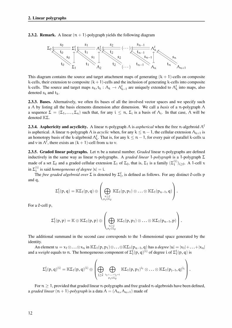
2.3.2. Remark. A linear (n+ 1)-polygraph yields the following diagram
Σ0 Σℓ1t0
oo
s0oo
Λℓ2t1
oo
s1oo (· · · )
t2oo
s2oo
Λℓntn−1
oo
sn−1oo
Σ1t0
ccGGGGGGGGGGGG
s0
ccGGGGGGGGGGGG OO
OO
Λ2t1
ccGGGGGGGGGGGG
s1
ccGGGGGGGGGGGG OO
OO
(· · · )t2
ddIIIIIIIIIIII
s2
ddIIIIIIIIIIII
Λntn−1
ddIIIIIIIIIIII
sn−1
ddIIIIIIIIIIII OO
OO
Λn+1tn
ddIIIIIIIIIIII
sn
ddIIIIIIIIIIII
This diagram contains the source and target attachment maps of generating (k + 1)-cells on composite
k-cells, their extension to composite (k+ 1)-cells and the inclusion of generating k-cells into composite
k-cells. The source and target maps sk, tk : Λk → Λℓk−1 are uniquely extended to Λℓk into maps, also
denoted sk and tk.
2.3.3. Bases. Alternatively, we often fix bases of all the involved vector spaces and we specify such
a Λ by listing all the basis elements dimension after dimension. We call a basis of a n-polygraph Λ
a sequence Σ = (Σ1, . . . , Σn) such that, for any i ≤ n, Σi is a basis of Λi. In that case, Λ will be
denoted KΣ.
2.3.4. Asphericity and acyclicity. A linear n-polygraph Λ is aspherical when the free n-algebroid Λℓ
is aspherical. A linear n-polygraph Λ is acyclic when, for any k ≤ n− 1, the cellular extension Λk+1 is
an homotopy basis of the k-algebroid Λℓk. That is, for any k ≤ n− 1, for every pair of parallel k-cells u
and v in Λℓ, there exists an (k+ 1)-cell from u to v.
2.3.5. Graded linear polygraphs. Let n be a natural number. Graded linear n-polygraphs are defined
inductively in the same way as linear n-polygraphs. A graded linear 1-polygraph is a 1-polygraph Σ
made of a set Σ0 and a graded cellular extension Σ1 of Σ0, that is, Σ1 is a family (Σ(i)1 )i≥0. A 1-cell x
in Σ(i)1 is said homogeneous of degree |x| = i.
The free graded algebroid over Σ is denoted by Σℓ1, is defined as follows. For any distinct 0-cells p
and q,
Σℓ1(p, q) = KΣ1(p, q)⊕
⊕
n≥2pi∈Σ0
KΣ1(p, p1)⊗ . . .⊗KΣ1(pn−1, q)
.
For a 0-cell p,
Σℓ1(p, p) = K⊕KΣ1(p, p)⊕
⊕
n≥2pi∈Σ0
KΣ1(p, p1)⊗ . . .⊗KΣ1(pn−1, p)
.
The additional summand in the second case corresponds to the 1-dimensional space generated by the
identity.
An element u = x1⊗ . . .⊗xn in KΣ1(p, p1)⊗ . . .⊗KΣ1(pn−1, q) has a degree |u| = |x1|+ . . .+ |xn|
and a weight equals to n. The homogeneous component of Σℓ1(p, q)(i) of degree i of Σℓ1(p, q) is
Σℓ1(p, q)(i) = KΣ1(p, q)
(i) ⊕
⊕
j≥2
⊕
i1+...+ij=i
pi∈Σ0
KΣ1(p, p1)i1 ⊗ . . .⊗KΣ1(pj−1, q)
ij
.
For n ≥ 1, provided that graded linear n-polygraphs and free gradedn-algebroids have been defined,
a graded linear (n+ 1)-polygraph is a data Λ = (Λn, Λn+1) made of
12
3. Two-dimensional linear rewriting systems
i) a graded linear n-polygraph Λn =(Σ0, (Σ
(i)1 )i≥0, . . . , (Λ
(i)n )i≥0
),
ii) a linear cellular extension Λn+1 = (Λ(i)n+1)i≥0 of the free graded n-algebroid Λℓn:
Λℓn = Σℓ1[Λ2] · · · [Λn].
The free graded (n+ 1)-algebroid over Λ is defined as Λℓn+1 = Λℓn[Λn+1].
Note that, as the source and target maps are graded, any k-sphere (f, g) is homogeneous, in the sense
that the k-cells f and g have the same degree. It follows that the linear cellular extensions have a natural
induced grading; an element (f, g) of Λk such that f and g are of degree i is a called a homogeneous
k-cell of Λ of degree i.
When Σ1 is concentrated in degree 1, then the notions of degree and weight coincide. Unless it is
specified, we will suppose that the 1-cells in Σ1 are concentrated in degree 1.
2.3.6. Homogeneous polygraphs. Let ω : N→ N be a (degree) function. We said that a graded linear
n-polygraph Λ is ω-concentrated if for any 1 ≤ k ≤ n, Λk is concentrated in degree ω(k), that is for
any k-cell f, |sk−1(f)| = |tk−1(f)| = ω(k). We will use the degree function ℓN, where N ≥ 2 is an
integer, defined by
ℓN(k) =
{lN if k = 2l,
lN+ 1 if k = 2l+ 1,
for any integer k ≥ 0. A n-polygraph is said to be N-homogeneous, or N-diagonal, if it is
ℓN-concentrated. In particular, an N-homogeneous linear 2-polygraph is a graded linear 2-polygraph,
such that any 2-cell has the form ∑
j∈J
λjmj ⇒∑
i∈I
λimi,
where |mj| = |mi| = N, for any i and j. We will say quadratic (resp. cubical) for 2-homogeneous (resp.
3-homogeneous) 2-polygraph.
2.3.7. Presentations of algebroids. A presentation of an algebroid A is a linear 2-polygraph Λ such
that A is isomorphic to the quotient algebroid Σℓ1/Λ2. In the case where A has exactly one 0-cell, the
notion coincides with the usual notion of presentation of A, as the free algebra generated by the set Σ1quotiented by the space of relations Λ2. We will denote by Λ the algebroid presented by a linear 2-
polygraph Λ. We denote by u the image of a 1-cell u in Σℓ1 by the canonical projection Σℓ1 → Λ. An
algebroid is said to beN-homogeneous if it is presented by aN-homogeneous linear 2-polygraphΛ, that
is, for any 2-cell f in Λ, we have |s1(f)| = |t1(f)| = N. The relations of A being N-homogeneous, the
algebroid A is equipped with a degree grading. The usual homological notions related to the algebroid A
can be equipped with this additional degree grading.
2.3.8. Tietze equivalence. Two linear n-polygraphs Λ and ∆ are said to be Tietze equivalent if they
present the same algebroid, that is, there is an isomorphism of algebroids Λ ≃ ∆.
3. TWO-DIMENSIONAL LINEAR REWRITING SYSTEMS
3.1. Linear 2-polygraph
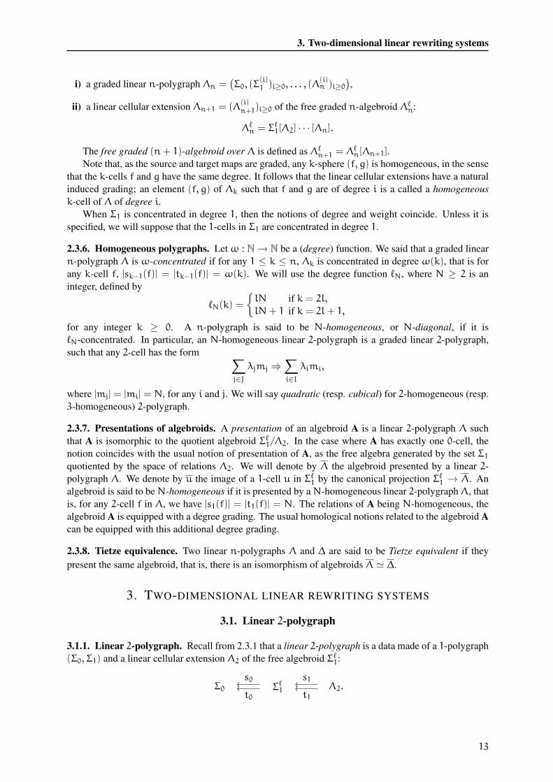
3.1.1. Linear 2-polygraph. Recall from 2.3.1 that a linear 2-polygraph is a data made of a 1-polygraph
(Σ0, Σ1) and a linear cellular extension Λ2 of the free algebroid Σℓ1:
Σ0 Σℓ1t0
oo
s0oo Λ2.
t1oo
s1oo
13
3. Two-dimensional linear rewriting systems
Suppose that Σ1 is a finite set {x1, . . . , xk}. The 1-cells in the free 1-category Σ∗1 are called monomial
1-cells in the variables x1, . . . , xk. The 1-cells in the free algebroid Σℓ1 are polynomials 1-cells in the
variables x1, . . . , xk. Any 1-cell f in Σℓ1 can be written uniquely as a linear sum:
f =∑
i∈I
λimi,
where, for any i ∈ I, λi are non-zero scalars and themi are pairwise distinct non-zero monomial 1-cells.
Such a decomposition is called a reduced expression of the 1-cell f with respect to the basis Σ1.
3.1.2. Monic linear 2-polygraph. A linear 2-polygraphΛ is said to be monic if it has a basis (Σ0, Σ1, Σ2)
such that any 2-cell in Σ2 has a non-zero monomial source. That is, any 2-cell in Σ2 has the form
α : m⇒∑
i∈I
λimi,
where m and the mi’s, for any i ∈ I, are non-zero monomial 1-cells. Obviously, any linear 2-polygraph
is Tietze equivalent to a monic linear 2-polygraph. Note that any 2-polygraph can be viewed as a monic
linear 2-polygraph for which the target of any 2-cell is also monomial.
3.2. Rewriting properties of linear 2-polygraphs
In this section, Λ denotes a monic linear 2-polygraph with basis (Σ0, Σ1, Σ2).
The notion of rewriting step induced byΛ needs to be defined with attention owing to the invertibility
of 2-cells in the free algebroid Λℓ2. Indeed, given a rule ϕ : m ⇒ h in Λ2, we have in the 2-algebroid
Λℓ2 the 2-cell −ϕ : −m ⇒ −h hence the 2-cell −ϕ + (m + h) : h ⇒ m. It is useless to hope for
termination if we consider all the 2-cells of Λℓ2 as rewriting sequences. We define a rewriting step as the
application of a rule on a reduced 1-cell, eg. −m+ (m+h) is not reduced, thus −ϕ+ (m+h) will not
considered as a rewriting step.
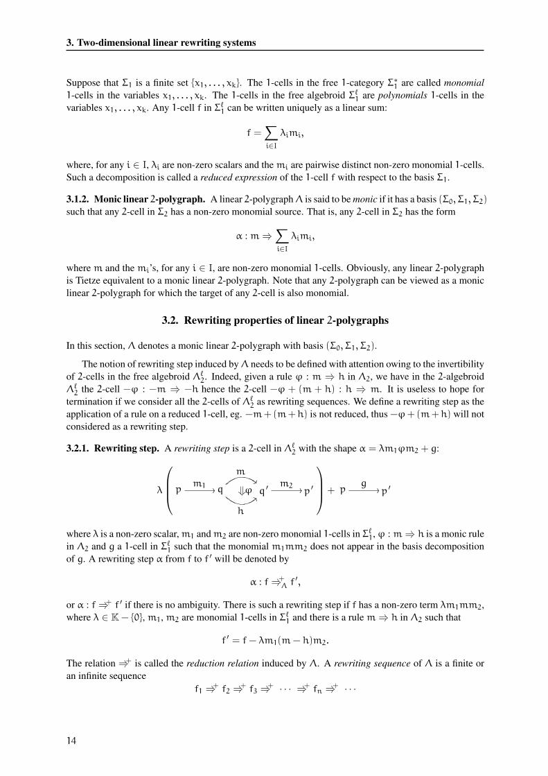
3.2.1. Rewriting step. A rewriting step is a 2-cell in Λℓ2 with the shape α = λm1ϕm2 + g:
λ
p
m1// q
m""
h
<<ϕ�� q ′
m2// p ′
+ p
g// p ′
where λ is a non-zero scalar,m1 andm2 are non-zero monomial 1-cells in Σℓ1,ϕ : m⇒ h is a monic rule
in Λ2 and g a 1-cell in Σℓ1 such that the monomial m1mm2 does not appear in the basis decomposition
of g. A rewriting step α from f to f ′ will be denoted by
α : f⇒+Λ f
′,
or α : f⇒+ f ′ if there is no ambiguity. There is such a rewriting step if f has a non-zero term λm1mm2,
where λ ∈ K− {0},m1,m2 are monomial 1-cells in Σℓ1 and there is a rulem⇒ h in Λ2 such that
f ′ = f− λm1(m− h)m2.
The relation⇒+ is called the reduction relation induced by Λ. A rewriting sequence of Λ is a finite or
an infinite sequence
f1 ⇒+ f2 ⇒+ f3 ⇒+ · · · ⇒+ fn ⇒+ · · ·
14
3.2. Rewriting properties of linear 2-polygraphs
of rewriting steps. If there is a non-empty rewriting sequence from f to g, we say that f rewrites into g
and we denote f⇒∗Λ g, or f⇒∗ g if there is no confusion.
We denote by Λ+2 (resp. Λ+f
2 ) the set of (resp. finite) rewriting sequences of Λ, also called positive
2-cells of the linear 2-polygraph Λ. Note that the free 2-groupoid on Λ+f2 is the 2-algebroid Λℓ2.
We denote f ⇔∗Λ g, or f ⇔∗ g, when there exists a finite zigzag of rewriting steps between f and g,
that is when there exist 1-cells f1, . . . , fp such that fi ⇒+ fi+1 or fi+1 ⇒+ fi for 1 ≤ i < p, with f1 = f
and fp = g.
3.2.2. Ideal generated by a linear 2-polygraph. We denote by I(Λ) the two-sided ideal of the alge-
broid Σℓ1 generated by the set
{ m− h | m⇒ h ∈ Λ2 }.
Given 1-cells f and f ′ in Σℓ1, there is a 2-cell f⇒ f ′ in Λℓ2 if and only if f− f ′ ∈ I(Λ). In particular, for
a 1-cell f in Σℓ1, we have
f⇔∗ 0 if and only if f ∈ I(Λ).
3.2.3. Normal forms. A 1-cell f of Σℓ1 is irreducible when there is no rewriting step of Λ with source f.
In particular a zero 1-cell is irreducible. A normal form of f is an irreducible 1-cell g such that f rewrites
into g. A 1-cell in Σℓ1 is reducible if it is not irreducible. We denote by ir(Λ) (resp. irm(Λ)) the set
of irreducible polynomial (resp. monomial) 1-cells for Λ. The set ir(Λ) forms a vector space ; the
polygraph Λ being monic, it is generated by irm(Λ).
3.2.4. Termination. We say that Λ is terminating when it has no infinite rewriting sequence. In that
case, every 1-cell in Σℓ1 has at least one normal form. Moreover, Noetherian induction, also called well-
founded induction, allows definitions and proofs of properties of 1-cells by induction on the number of
rewriting steps reducing a 1-cell to a normal form.
When Λ is terminating, as a vector space, the algebroid Σℓ1 has the following decomposition
Σℓ1 = ir(Λ) + I(Λ).
This decomposition is proved by induction on monomial 1-cells. Let m be a monomial 1-cell in Σℓ1. If
m is irreducible, then m = m + 0, else it can be written m = m1m′m2, where m ′ is the source of a
2-cell m ′ ⇒ h in Λ2. The polynomial f = m1(m′ − h)m2 is in I(Λ) and we have f = m −m1hm2.
By induction, there is a decomposition m1hm2 = hir + hI, with hir irreducible and hI in I(Λ). Then
m = hir + (f+ hI). This proves the decomposition.
3.2.5. Methods to prove termination. One idea to prove the termination of a linear 2-polygraph is to
associate a 2-polygraph whose termination can be proven using usual techniques on 2-polygraphs. Given
a basis of Λ2 by cells of the form
α : m⇒∑
i∈Im
λimi
where the λi are non-zero scalars, the associated 2-polygraph T(Λ) is defined by T(Λ) = (Σ0, Σ1,T(Λ)2)
where T(Λ)2 is defined by ⋃
m
{m⇒ mi, i ∈ Im}.
We suppose moreover that any monomialm is the source of a finite number of 2-cells.
3.2.6. Proposition. If T(Λ) is terminating, then Λ is terminating.
Proof. To any rewriting sequence in Λ starting with a monomial m in Σℓ1, we associate a tree labelled
by monomials in Σℓ1 as follows:
15
3. Two-dimensional linear rewriting systems
- The root vertex of the tree ism.
- If a vertex v is at some point during the rewriting sequence, rewritten into a linear combination of
monomials vi’s, then in the tree, the vertices labelled by v have outgoing edges to vertices labelled
by vi.
Note that in this tree, every edge corresponds to a rewriting step in T(Λ). Suppose now that Λ is
not terminating, that is there exists an infinite rewriting sequence in Λ. Then the associated tree has an
infinite number of vertices, and therefore has a monotonous path of infinite length starting at the root.
This implies that T(Λ) is not terminating.
Proposition 3.2.6 implies that the usual methods to prove termination in the usual context can be used
to prove termination in the linear context.
We now study the notion of confluence of linear 2-polygraphs, to study what happens when a mono-
mial 1-cell is the source of more than one rewriting step.
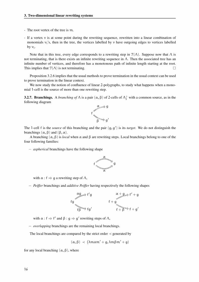
3.2.7. Branchings. A branching of Λ is a pair (α,β) of 2-cells of Λ+2 with a common source, as in the
following diagram
g
f
α %9
β#7 g ′
The 1-cell f is the source of this branching and the pair (g, g ′) is its target. We do not distinguish the
branchings (α,β) and (β,α).
A branching (α,β) is local when α and β are rewriting steps. Local branchings belong to one of the
four following families:
− aspherical branchings have the following shape
f
α�,
α
2F g
with α : f⇒ g a rewriting step of Λ,
− Peiffer branchings and additive Peiffer having respectively the following shapes
f ′g
fg
αg ';
fβ#7 fg ′
f ′ + g
f+ g
α+ g ';
f+ β#7 f+ g ′
with α : f⇒ f ′ and β : g⇒ g ′ rewriting steps of Λ,
− overlapping branchings are the remaining local branchings.
The local branchings are compared by the strict order ≺ generated by
(α,β) ≺(λmαm ′ + g, λmβm ′ + g)
for any local branching (α,β), where
16
3.2. Rewriting properties of linear 2-polygraphs
1. λ is in K \ {0},
2. m andm ′ are monomial 1-cells such thatmαm ′ exists (and, thus, so doesmβm ′),
3. g is in Σℓ1,
4. no monomial in the basis decomposition of g appears in the basis decomposition ofms(α)m ′,
5. and at least one of the two following conditions is satisfied
(i) eitherm orm ′ is not an identity monomial.
(ii) g is not zero.
An overlapping local branching that is minimal for the order ≺ is called a critical branching. If
(α,β) is a critical branching, the difference t1(α) − t1(β) is called the S-polynomial of the critical
branching (α,β). Note that a critical branching has a monomial source.
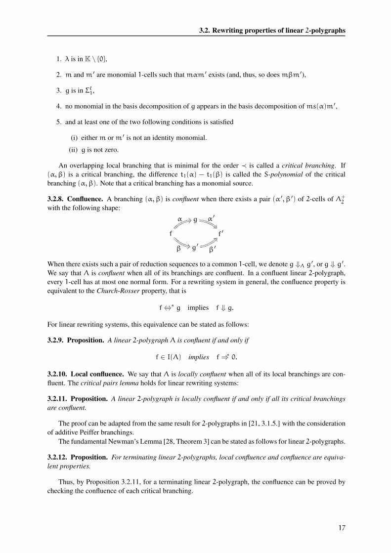
3.2.8. Confluence. A branching (α,β) is confluent when there exists a pair (α ′, β ′) of 2-cells of Λ+2
with the following shape:
g α ′
�)f
α &:
β"6
f ′
g ′β ′
6J
When there exists such a pair of reduction sequences to a common 1-cell, we denote g ⇓Λ g ′, or g ⇓ g ′.
We say that Λ is confluent when all of its branchings are confluent. In a confluent linear 2-polygraph,
every 1-cell has at most one normal form. For a rewriting system in general, the confluence property is
equivalent to the Church-Rosser property, that is
f⇔∗ g implies f ⇓ g.
For linear rewriting systems, this equivalence can be stated as follows:
3.2.9. Proposition. A linear 2-polygraph Λ is confluent if and only if
f ∈ I(Λ) implies f⇒∗ 0.
3.2.10. Local confluence. We say that Λ is locally confluent when all of its local branchings are con-
fluent. The critical pairs lemma holds for linear rewriting systems:
3.2.11. Proposition. A linear 2-polygraph is locally confluent if and only if all its critical branchings
are confluent.
The proof can be adapted from the same result for 2-polygraphs in [21, 3.1.5.] with the consideration
of additive Peiffer branchings.
The fundamental Newman’s Lemma [28, Theorem 3] can be stated as follows for linear 2-polygraphs.
3.2.12. Proposition. For terminating linear 2-polygraphs, local confluence and confluence are equiva-
lent properties.
Thus, by Proposition 3.2.11, for a terminating linear 2-polygraph, the confluence can be proved by
checking the confluence of each critical branching.
17
3. Two-dimensional linear rewriting systems
3.2.13. Convergence. A linear 2-polygraph is said to be convergent when it terminates and is confluent.
In that case, every 1-cell f has a unique normal form, denoted f. Such a Λ is called a convergent
presentation of the algebroid Λ presented by Λ. In that case, there is a canonical section Λ → Σℓ1sending f to its normal form f, so that f = g holds in Σℓ1 if, and only if, we have f = g in Λ. As
a consequence, a finite and convergent linear 2-polygraph Λ yields generators for the 1-cells of the 1-
algebroid Λ, together with a decision procedure for the corresponding word problem. The finiteness is
used to effectively check that a given 1-cell is a normal form.
We end this section with a criterion to prove confluence of terminating polygraphs, like the Buch-
berger criterion for Gröbner bases.
3.2.14. Proposition. Let Λ be a terminating linear 2-polygraph.
i) For any 1-cells g and g ′, if g− g ′ ⇒∗ 0, then g ⇓ g ′.
ii) Λ is confluent if and only if the S-polynomial of every critical branching is reduced to 0.
Proof. Let Λ be terminating. The proof of i) is made by Noetherian induction, as in [4, Lemma 8.3.3] or
[23, Lemma 2.2.].
Prove ii). Suppose that Λ is confluent, then any critical branching (α,β) is confluent. Thus there
exists reductions α ′ : t1(α) ⇒∗ f ′ and β ′ : t1(β) ⇒∗ f ′, hence the S-polynomial t1(α) − t1(β) is
reduced to 0. Conversely, suppose that the S-polynomial of every critical branching is reduced to 0. By
Propositions 3.2.12 and 3.2.11, it suffices to prove that every critical branching in Λ is confluent. Let
(α,β) be a critical branching of source f, with t1(α) = g and t1(β) = g ′. We have g − g ′ ⇒∗ 0, and
we conclude by i).
3.3. The basis of irreducibles
In this section, Λ denotes a monic linear 2-polygraph (Σ0, Σ1, Λ2).
3.3.1. Bases of irreducibles. The decomposition Σℓ1 = ir(Λ) + I(Λ) obtained in 3.2.4 is not direct in
general. Suppose that Λ is convergent and consider the projection
π : Σℓ1// // ir(Λ)
sending a polynomial f on its unique normal form. By Proposition 3.2.9, we have π(f) = 0 if and only
if f is in I(Λ). Thus we have a family of exact sequences of vector spaces
0 // I(Λ)(p,q)�
�
// Σ1ℓ(p,q)
π(p,q)// // ir(Λ)(p,q) // 0
indexed by 0-cells p, q in A0. Thus the maps π(p,q) induce an isomorphism of vector spaces from the
algebroidΛ to ir(Λ). In this situation, we call the map π a linear isomorphism, that is a map of algebroids
which is an isomorphism of vector spaces.
As a consequence, we have
3.3.2. Proposition. Let Λ be a terminating linear 2-polygraph. Then Λ is confluent if and only if the
decomposition is direct:
Σℓ1 = ir(Λ)⊕ I(Λ).
Proof. Suppose Λ terminating, by 3.2.4, we have the decomposition Σℓ1 = ir(Λ) + I(Λ). By Proposi-
tion 3.2.9, the polygraph Λ is confluent if and only if, for any f ∈ I(Λ), f ⇒∗ 0. It follows that Λ is
confluent if and only if ir(Λ) ∩ I(Λ) = {0}, hence the decomposition is direct.
18
3.3. The basis of irreducibles
3.3.3. Standard bases. As a consequence, when Λ is convergent, the set of irreducible monomials
irm(Λ) forms a K-linear basis of the algebroid Λ via the canonical map ir(Λ) −→ Λ, called a standard
basis of A. Moreover, with the multiplication on ir(Λ) defined by
f · g = π(fg),
for any f and g in ir(Λ), then ir(Λ) is isomorphic to the algebroid Λ.
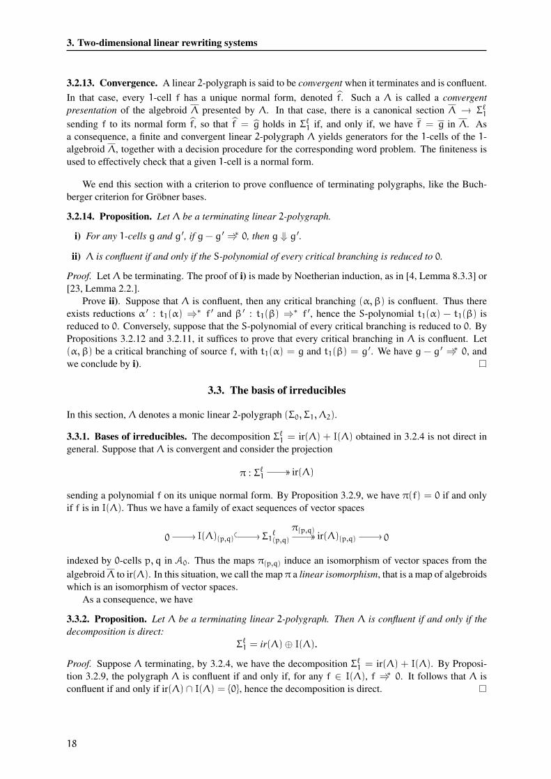
3.3.4. Example. Consider the algebra A〈 x, y | xy = x2 〉. The presentation by the polygraph Λ
defined by the 2-cell xy ⇒ x2 is confluent, because there is no critical branching. Hence, the set of
normal forms irm(Λ) = {yixj | i, j ∈ N} forms a basis of algebra A. However, the polygraph Λ ′ with
the 2-cell x2 ⇒ xy is a non convergent presentation of A ; there is a non-confluent critical branching:
xyx
x3
/Cssssssss
�.HHHHHHHH
x2y %9 xy2
The monomials xyx and xy2 in irm(Λ′) are equal in A, thus are not linearly independant.
3.3.5. Monomial algebras. We associate to a monic linear 2-polygraphΛ the linear 2-polygraph M(Λ) =
(Σ0, Σ1,M(Λ)2), whose 2-cells are defined by
M(Λ)2 = { s1(α)⇒ 0 | α ∈ Λ2 }.
Following 3.3.2, if Λ is convergent, there is a linear isomorphism Λ ≃ M(Λ). A linear basis of the
algebroid M(Λ) is given by the monomial 1-cells in Σℓ1 not reducible by a 2-cell in Λ2.
3.3.6. Poincaré-Birkhoff-Witt bases. Let A be anN-homogeneous algebroid and letΛ = (Σ0, Σ1, Λ2)
be a monicN-homogeneous presentation of A. A set Ξ1 of 1-cells in Σ∗1 is called a Poincaré-Birkhoff-Witt
basis, PBW for short, of A if the three following conditions are satisfied:
i) For all 0-cells p and q, there is an isomorphism of vector spaces KΞ1(p, q) ≃ A(p, q).
ii) For 0-composable 1-cells u and v in Ξ, the 0-composition uv is either in Ξ1 or reducible by Λ2.
iii) For any natural number p and any 0-composable 1-cells v1, . . . , vp, the 0-composition v1 . . . vp is
in Ξ1 if, and only if, for all 1 ≤ k ≤ p−N+ 1, the 0-composition vk . . . vk+N−1 is in Ξ1.
When Λ is convergent, the associated standard basis is a PBW basis.
3.3.7. Proposition. If Λ is N-homogeneous and convergent, then the standard basis irm(Λ) is a PBW
basis of the algebroid A.
Conversely, suppose that an N-homogeneous algebroid A presented by (Σ0, Σ1, Λ2) admits a PBW
basis Ξ1. For any 0-composable 1-cells u and v in Ξ1, we denote by [uv]Ξ1 the linear decomposition of
the 1-cell uv in the basis Ξ1. Let us define
Ξ2 = { uv⇒ [uv]Ξ1 | u, v in Ξ1 and |uv| = N }.
Let Ξ be the 2-linear polygraph Ξ defined by (Σ0, Ξ1, Ξ2).
3.3.8. Proposition. If Ξ terminates, the 2-linear polygraph Ξ is a convergent presentation of A.
19
3. Two-dimensional linear rewriting systems
Proof. First, note that any monomial 1-cell of degree N can be expressed as the 0-composite of two
monomials of degree smaller than N, thus which are in Ξ1. This observation implies that all relations in
Λ2 are in Ξ2. Thus the algebroid presented by Ξ surjects (as an algebroid) to A. Moreover, by definition,
Ξ and Λ have the same irreducible monomials. As Ξ terminates, these monomials form the standard
basis of the algebroid presented by Ξ. This implies that Ξ is a presentation of A.
Let us show now that Ξ is convergent. It is enough to prove that for any monomials u and v in Σℓ1such that u = v in A, u and v can be rewritten using Ξ to the same w in KΞ1. Suppose that u is not in
Ξ1. Then by the third property of a PBW basis, we can find a subword u ′ of u of degree N that is not
in Ξ1. This subword can be expressed as the 0-composite of two monomials of degree smaller than N,
thus which are in Ξ1. Thus, by the second property of a PBW basis, u ′ is reducible by Ξ2. Therefore
u⇒Ξ
∑λiui such that u =
∑λiui. If some ui is not in Ξ1, we can iterate this process until we obtain
u ⇒∗Ξ wu where wu is in KΞ1 and u = wu. Note that this process is finite as Ξ terminates. Similarly,
we obtain that v ⇒∗Ξ wv where wv is in KΞ1 and v = wv. But as v = u, we obtain wu = wv, which
implies wu = wv as Ξ1 is a basis of A.
3.4. Associative Gröbner bases
In this section, we show how the Gröbner bases correspond to convergent linear 2-polygraphs. Through-
out this section, (Σ0, Σ1) denotes a 1-polygraph.
3.4.1. Monomial order. Let us fix a monomial order ≺ on Σ∗1, that is a well-order compatible with the
associative product. Explicitly, it is a strict total order ≺ on Σ∗1 such that there is no infinite decreasing
sequence and m1 ≺ m2 implies mm1n ≺ mm2n, for any monomials m and n in Σ∗1. Any non-zero
1-cell f in Σℓ1 can be uniquely written
f = λ1m1 + . . .+ λpmp,
wherem1, . . . ,mp are pairwise distinct monomials 1-cells and λi ∈ K− {0}, for any i ∈ I = {1, . . . , p}.
The leading term of f, denoted lt(f), is the polynomial λjmj, such that mi ≺ mj, for any i ∈ I − {j}.
Then we say that λj is the leading coefficient of f, denoted lc(f) and mj is the leading monomial of f,
denoted lm(f). We also define lt(0) = lc(0) = lm(0) = 0.
3.4.2. Well-ordered linear 2-polygraphs. A monomial order ≺ on Σ∗1 induces a partial order on the
free algebroid Σℓ1, also denoted by ≺, defined by
i) for any non-zero 1-cell f, 0 ≺ f,
ii) for non-zero 1-cells f and g, define g ≺ f if, and only if, either lm(g) ≺ lm(f) or (lm(g) = lm(f)
and g− lt(g) ≺ f− lt(f)).
In this way, the partial order ≺ on Σℓ1 is well-founded and compatible with associative product.
A linear cellular extension Λ2 of Σℓ1 is said to be compatible with the monomial order ≺, if for
any 2-cell m ⇒ u in Λ2, we have u ≺ m. A well-ordered linear 2-polygraph is a linear 2-polygraph
(Σ0, Σ1, Λ2) together with a monomial order on Σ∗1 and whose cellular extension Λ2 is compatible with
this monomial order. Note that a well-ordered linear 2-polygraph is always terminating.
3.4.3. Polynomial 2-linear polygraphs. Let ≺ be a monomial order on Σ∗1. Given a non-zero 1-cell g
in Λℓ1. The polynomial reduction by g is the monic 2-cell defined by
αg : lm(g)⇒ lm(g) −1
lc(g)g.
20
3.4. Associative Gröbner bases
For a set of non-zero 1-cells G in Σℓ1, we denote by Λ(G) the linear 2-polygraph whose generating 2-
cells are the 2-cells αg, for g in G. Note that the reduction in Λ(G) is by definition compatible with the
monomial order ≺, hence the linear polygraph Λ(G) is terminating.
3.4.4. Gröbner bases. Given a monomial order on Σ∗1 and I an ideal in Σℓ1, a Gröbner basis of I is a
subset G of I such that, for any 1-cell f in I, there exists g in G such that lt(f) = mlt(g)m ′, where m
and m ′ are non-zero monomial 1-cells. That is, the two-sided ideal generated by the leading terms of
1-cells in I coincide with the two-sided ideal generated by the leading terms of elements in G:
〈 lt(I) 〉 = 〈 lt(G) 〉.
3.4.5. S-polynomials. Suppose that g1 and g2 are two non-zero 1-cells in Σℓ1 such that their leading
monomials have a small common multiple h, i.e. such that there are monomial 1-cells m and m ′ such
that h = lm(g1)m = m ′lm(g2). We define the S-polynomial of the polynomial 1-cells g1 and g2 as the
S-polynomial of the critical branching (αg1 , αg2), that is
S(g1, g2) =1
lc(g1)g1m−
1
lc(g2)m ′g2.
By construction, we have lm(S(g1, g2)) < lm(h) = h.
We recall here the Buchberger criterion for Gröbner bases.
3.4.6. Proposition. LetΣ1 be a 1-polygraph and let ≺ be a monomial order onΣ∗1. LetG = {g1, . . . , gk}
be a finite set of polynomials and let I(G) be the ideal of Σℓ1 generated by G. The following conditions
are equivalents:
i) G is a Gröbner basis of I(G),
ii) for any g1 and g2 in G, S(g1, g2)⇒∗Λ(G) 0,
iii) the linear 2-polygraph Λ(G) is confluent.
Proof. The equivalence i) <=>ii) is standard, see for instance [19, Theorem 2.3]. Note that the critical
pairs ofΛ(G) are of the form (αg1 , αg2) such that the monomials lm(g1) and lm(g2) overlap as in 3.4.5.
By ii) of Proposition 3.2.14, the polygraph Λ(G) is confluent if and only if the S-polynomial of each
such a critical pair is reduced to 0. This proves the equivalence between ii) and iii).
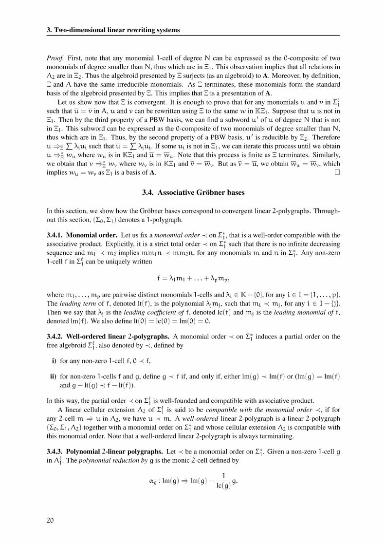
3.4.7. Example. Consider the algebra given by the following presentation
A〈 x, y, z | xyz = x3 + y3 + z3 〉.
With the lexicographic order induced by x < y < z, the ideal generated by the relation admits the
Gröbner basis with two elements corresponding to the following two rules:
z3α %9 xyz− x3 − y3, zy3
β %9 zxyz− zx3 − xyz2 + x3z+ y3z.
With such a presentation, Anick’s resolution is infinite ; the Anick’s chains are of the form zn and zny3,
with n ≥ 0. It is possible to consider another presentation of the algebra A, with the rule
xyzγ %9 x3 + y3 + z3.
This presentation is confluent, as it has no critical branching. Moreover, it is terminating, as for each
monomial, the quantity 3A + B decreases when we apply the rewriting rule, where A is the number of
occurrences of the product xyz and B the number of occurences of y.
21
4. Polygraphic resolutions of algebroids
4. POLYGRAPHIC RESOLUTIONS OF ALGEBROIDS
In this section, we introduce the notion of polygraphic resolution for algebroids. We show how to con-
struct such a resolution from a convergent presentation. Our construction consists in extending a reduced
monic linear 2-polygraph Λ into a polygraphic resolution of the presented algebroid, whose generating
n-cells, for n ≥ 3, are indexed by the (n− 1)-fold critical branchings of Λ.
Throughout this section, A denotes an algebroid.
4.1. Polygraphic resolutions of algebroids and normalisation strategies
4.1.1. Polygraphic resolutions of algebroids. A polygraphic resolution (resp. graded polygraphic
resolution) of A is an acyclic linear∞-polygraph (resp. graded acyclic linear∞-polygraph) Λ, whose
underlying linear 2-polygraph Λ2 is a presentation of A. For a natural integer n, such that 2 ≤ n < ∞,
a partial polygraphic resolution of length n of A is an acyclic linear n-polygraph Λ, whose underlying
linear 2-polygraph is a presentation of A.
When f is a k-cell of Λ, for k ≥ 2, we will denote by f the 1-cell s1(f) = t1(f) in A.
4.1.2. N-homogeneous resolution. Given a degree function ω : N → N, a graded polygraphic resolu-
tion Λ isω-concentrated (resp. N-homogeneous) when the linear polygraph Λ isω-concentrated (resp.
ℓN - concentrated).
4.1.3. Sections. Let us fix n ≥ 2 either a natural number or ∞. Let Λ = (Σ0, Σ1, Λ2, . . . , Λn) be a
linear n-polygraph, whose underlying linear 2-polygraph is a presentation of A.
A section of Λ is a choice of a representative 1-cell u : p → q in Σℓ1, for every 1-cell u : p → q of
A, such that 1p = 1p holds for every 0-cell p of A. Such an assignment is not assumed to be functorial
with respect to the 0-composition, but linear, that is for any 1-cells u and v and scalar λ in K, the section
satisfies:
u+ v = u+ v, λu = λu.
The assignment · : u 7→ u is extended in a unique way by precomposition with the canonical projection
Σℓ1 ։ A, into a map
· : Σℓ1 −→ Σℓ1
mapping each 1-cell u in Σℓ1 to a parallel 1-cell u in Σℓ1, in such a way that the equality u = v holds in A
if, and only if, we have u = v in Σℓ1.
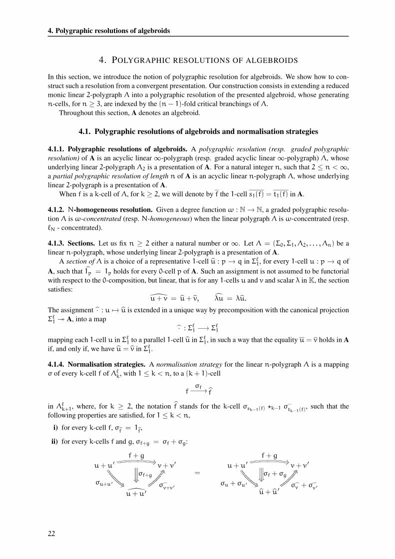
4.1.4. Normalisation strategies. A normalisation strategy for the linear n-polygraph Λ is a mapping
σ of every k-cell f of Λℓk, with 1 ≤ k < n, to a (k+ 1)-cell
fσf
//f
in Λℓk+1, where, for k ≥ 2, the notation f stands for the k-cell σsk−1(f) ⋆k−1 σ−tk−1(f)
, such that the
following properties are satisfied, for 1 ≤ k < n,
i) for every k-cell f, σf= 1
f,
ii) for every k-cells f and g, σf+g = σf + σg:
u+ u ′
f+ g"6
σu+u ′ �/
v+ v ′
u+ u ′
σ−v+v ′
;Oσf+g���
=u+ u ′
f+ g"6
σu + σu ′ �/
v+ v ′
u+ u ′σ−v + σ−v ′
:Nσf + σg���
22
4.1. Polygraphic resolutions of algebroids and normalisation strategies
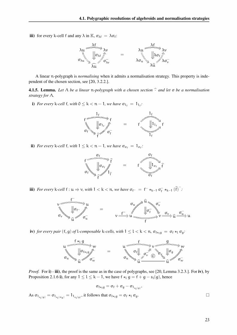
iii) for every k-cell f and any λ in K, σλf = λσf:
λuλf
4
σλu �-
λv
λu
σ−λv
@Tσλf���
=λu
λf 4
λσu �-
λv
λuλσ−v
@Tλσf���
A linear n-polygraph is normalising when it admits a normalisation strategy. This property is inde-
pendent of the chosen section, see [20, 3.2.2.].
4.1.5. Lemma. Let Λ be a linear n-polygraph with a chosen section · and let σ be a normalisation
strategy for Λ.
i) For every k-cell f, with 0 ≤ k < n− 1, we have σ1f = 11f:
f
1f 4
σf �0
f
fσ−f
?Sσ1f���
= f
1f
�(
1f
6J11f���f
ii) For every k-cell f, with 1 ≤ k < n− 1, we have σσf = 1σf:
f
σf 4
σf �/
f
f
1f
σσf���= f
σf
�(
σf
6J1σf��� f
iii) For every k-cell f : u⇒ v, with 1 < k < n, we have σf− = f− ⋆k−1 σ−f ⋆k−1 (f)
−:
vf−
!5
σv �1
u
uσ−u
=Qσf−���
=
uσ−v
� vf− %9 u
σu-A
f
)= vσ−f��� σv %9 u
σ−u %9 u
iv) for every pair (f, g) of l-composable k-cells, with 1 ≤ l < k < n, σf⋆lg = σf ⋆l σg:
u
f ⋆l g!5
σu �1
w
uσ−w
=Qσf⋆lg���
=u
f!5
σu �1
v
g!5
σv???
???
�)??????
w
u
σ−v����
5I����σf ��� c©
uσ−w
=Qσg���
Proof. For i) - iii), the proof is the same as in the case of polygraphs, see [20, Lemma 3.2.3.]. For iv), by
Proposition 2.1.6 i), for any 1 ≤ l ≤ k− 1, we have f ⋆l g = f+ g− sl(g), hence
σf⋆lg = σf + σg − σ1sl(g).
As σ1sl(g)= σ1sl(σg)
= 11sl(g), it follows that σf⋆lg = σf ⋆l σg.
23
4. Polygraphic resolutions of algebroids
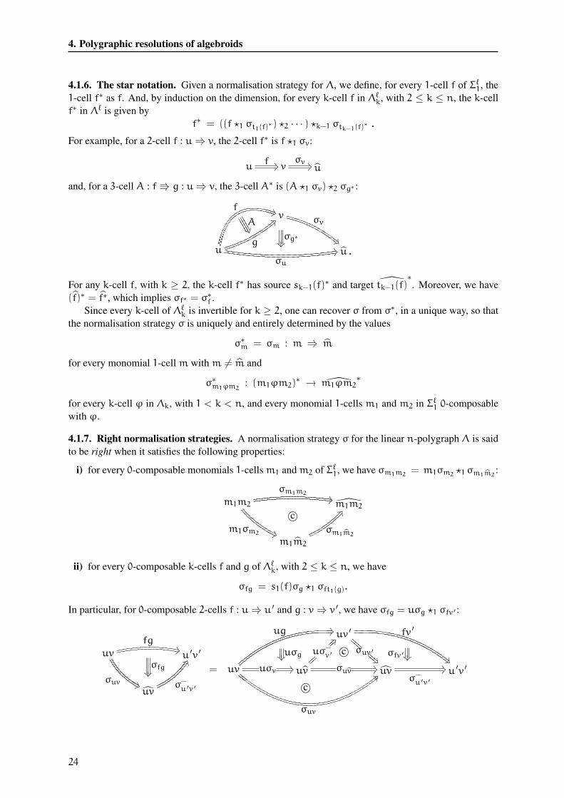
4.1.6. The star notation. Given a normalisation strategy for Λ, we define, for every 1-cell f of Σℓ1, the
1-cell f∗ as f. And, by induction on the dimension, for every k-cell f in Λℓk, with 2 ≤ k ≤ n, the k-cell
f∗ in Λℓ is given by
f∗ = ((f ⋆1 σt1(f)∗) ⋆2 · · · ) ⋆k−1 σtk−1(f)∗ .
For example, for a 2-cell f : u⇒ v, the 2-cell f∗ is f ⋆1 σv:
uf %9 v
σv %9 u
and, for a 3-cell A : f⇛ g : u⇒ v, the 3-cell A∗ is (A ⋆1 σv) ⋆2 σg∗ :
v σv
�+u
f �3
g
3G
σu
'; u .
A2�"2222
22222222
σg∗���
For any k-cell f, with k ≥ 2, the k-cell f∗ has source sk−1(f)∗ and target tk−1(f)
∗
. Moreover, we have
(f)∗ = f∗, which implies σf∗ = σ∗f .
Since every k-cell of Λℓk is invertible for k ≥ 2, one can recover σ from σ∗, in a unique way, so that
the normalisation strategy σ is uniquely and entirely determined by the values
σ∗m = σm : m ⇒ m
for every monomial 1-cellm withm 6= m and
σ∗m1ϕm2: (m1ϕm2)
∗ → m1ϕm2∗
for every k-cell ϕ in Λk, with 1 < k < n, and every monomial 1-cells m1 and m2 in Σℓ1 0-composable
with ϕ.
4.1.7. Right normalisation strategies. A normalisation strategy σ for the linear n-polygraph Λ is said
to be right when it satisfies the following properties:
i) for every 0-composable monomials 1-cellsm1 andm2 of Σℓ1, we have σm1m2= m1σm2
⋆1 σm1m2:
m1m2
σm1m2#7
m1σm2 �2
m1m2
m1m2
σm1m2
7Kc©
ii) for every 0-composable k-cells f and g of Λℓk, with 2 ≤ k ≤ n, we have
σfg = s1(f)σg ⋆1 σft1(g).
In particular, for 0-composable 2-cells f : u⇒ u ′ and g : v⇒ v ′, we have σfg = uσg ⋆1 σfv ′ :
uv
fg"6
σuv �1
u ′v ′
uvσ−u ′v ′
:Nσfg��� =
uv ′ fv ′
�,σuv ′
CCCCCC
�+CCCCCC
uv
ug $8
uσv %9
σuv
2Fuv
uσ−v ′{{{{
3G{{{{
σuv %9 uvσ−u ′v ′
%9 u ′v ′
uσg��� σfv ′ ���c©
c©
24

4.2. Polygraphic resolutions from convergence
Note that by the additivity property of strategies, we deduce from i) that for every 0-composable 1-cells
f and g of Σℓ1, we have σfg = fσg ⋆1 σfg.
A linear n-polygraph is right normalising when it admits a right normalisation strategy. Normalising
and right normalising properties for linear polygraphs correspond to the same properties for (n, 1)-
polygraphs which are studied in [20, 3.2.]. In particular, we have
4.1.8. Proposition ([20, Corollary 3.3.5.]). LetΛ be a linear n-polygraph. Right normalisation strate-
gies on Λ are in bijective correspondence with the families
σϕm : ϕm → ϕm
and with the families
σ∗ϕm : (ϕm)∗ → ϕm∗
of (k+ 1)-cells, indexed by k-cells ϕ of Λk, for 1 ≤ k ≤ n− 1, and by monomial 1-cellsm of Σℓ1 which
are 0-composable with ϕ.
4.1.9. Proposition. Let Λ be a linear n-polygraph. Then Λ is acyclic if and only if Λ is right normal-
isating.
Proof. Let us recall the proof from [20, Theorem 3.3.6.]. Suppose that Λ admits a right normalisation
strategy σ. We consider a k-cell f in Λℓk, for some 1 < k < n. By definition, there is a (k + 1)-cell
σf : f ⇛ f. If g is a k-cell which is parallel to f, recall that f = g. Thus the (k + 1)-cell σf ⋆k σ−g of
Λℓk+1 has source f and target g:
u f%9
f
�#
g
;O
σf ��
σ−g��� ����
����
����
v
This proves that Λk+1 forms a homotopy basis of Λℓk. Hence Λ is acyclic.
Conversely, suppose that the linear polygraph Λ is acyclic and let us define a right normalisation
strategy σ for Λ. We choose a 2-cell
σxm : xm⇒ xm
for every 1-cell x in Σ1 and every monomial 1-cellm in Σℓ1 such that xm is defined. Then, for 2 ≤ k < n,
the polygraph Λ being acyclic, Λk+1 is a homotopy basis of Λℓk, there is a (k+ 1)-cell
σϕm : ϕm −→ ϕm
for every k-cell ϕ in Λk and every monomial 1-cell m in Σℓ1, such that ϕm is defined. The Proposi-
tion 4.1.8 concludes.
4.2. Polygraphic resolutions from convergence
4.2.1. Reduced linear 2-polygraphs. Let Λ be a linear 2-polygraph with basis Σ. We say that Λ is
left-reduced when, for every 2-cell ϕ : m⇒ f in Σ2, the 1-cellm is a normal form for Σ2 \ {ϕ}. We say
that Λ is right-reduced when for every 2-cell ϕ : m⇒ f in Σ2, the 1-cell f is a normal form for Σ2. The
linear polygraph Λ is said to be reduced when it is both left and right reduced.
25
4. Polygraphic resolutions of algebroids
4.2.2. The rightmost normalisation strategy. Let m be a monomial 1-cell in Σℓ1. We define a rela-
tion � on rewriting steps with source m as follows. If ϕ and ψ are 2-cells in Λ and if f = m1ϕm2 and
g = m ′1ψm
′2 have common sourcem, then we write f � g when |m1| ≤ |m ′
1|. As for 2-polygraphs, see
[20, Lemma 4.2.2.], the relation � induces a total ordering on the rewriting steps of Λ with sourcem.
Let m be a reducible monomial 1-cell of Σℓ1. The rightmost rewriting step on m is denoted by νmand defined as the maximum elements for � of the (finite, non-empty) set of rewriting steps of Λ with
sourcem. Ifm andm ′ are reducible 0-composable monomial 1-cells of Σℓ1, then we have:
νmm ′ = mνm ′ .
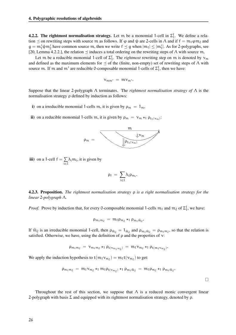
Suppose that the linear 2-polygraph Λ terminates. The rightmost normalisation strategy of Λ is the
normalisation strategy ρ defined by induction as follows:
i) on a irreducible monomial 1-cellsm, it is given by ρm = 1m,
ii) on a reducible monomial 1-cellsm, it is given by ρm = νm ⋆1 ρt1(νm):
ρm =
m//AA <<
νm��ρt1(νm)��
iii) on a 1-cell f =∑i∈I
λimi, it is given by
ρf =∑
i∈I
λiρmi.
4.2.3. Proposition. The rightmost normalisation strategy ρ is a right normalisation strategy for the
linear 2-polygraph Λ.
Proof. Prove by induction that, for every 0-composable monomial 1-cellsm1 andm2 of Σℓ1, we have:
ρm1m2= m1ρm2
⋆1 ρm1m2.
If m2 is an irreducible monomial 1-cell, then ρm2= 1m2
and ρm1m2= ρm1m2
, so that the relation is
satisfied. Otherwise, we have, using the definition of ρ and the properties of ν:
ρm1m2= νm1m2
⋆1 ρt(νm1m2) = m1νm2
⋆1 ρt(m1νm2).
We apply the induction hypothesis to t(m1νm2) = m1t(νm2
) to get:
ρm1m2= m1νm2
⋆1m1ρt(νm2) ⋆1 ρm1m2
= m1ρm2⋆1 ρm1m2
.
Throughout the rest of this section, we suppose that Λ is a reduced monic convergent linear
2-polygraph with basis Σ and equipped with its rightmost normalisation strategy, denoted by ρ.
26
4.2. Polygraphic resolutions from convergence
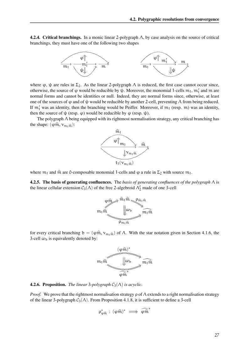
4.2.4. Critical branchings. In a monic linear 2-polygraph Λ, by case analysis on the source of critical
branchings, they must have one of the following two shapes
m1
// m ′1
//FF m
//
ϕEY
ψ ��
m1
//��m ′
1//
BBm
//
ϕEY
ψ��
where ϕ, ψ are rules in Σ2. As the linear 2-polygraph Λ is reduced, the first case cannot occur since,
otherwise, the source of ϕ would be reducible by ψ. Moreover, the monomial 1-cellsm1,m′1 andm are
normal forms and cannot be identities or null. Indeed, they are normal forms since, otherwise, at least
one of the sources ofϕ and ofψ would be reducible by another 2-cell, preventingΛ from being reduced.
If m ′1 was an identity, then the branching would be Peiffer. Moreover, if m1 (resp. m) was an identity,
then the source of ψ (resp. ϕ) would be reducible by ϕ (resp. ψ).
The polygraphΛ being equipped with its rightmost normalisation strategy, any critical branching has
the shape: (ϕm, νm1m):
m1//
m1
��
t1(νm1m)
>>m
//
ϕEY
νm1m��
wherem1 and m are 0-composable monomial 1-cells and ϕ a rule in Σ2 with sourcem1.
4.2.5. The basis of generating confluences. The basis of generating confluences of the polygraph Λ is
the linear cellular extension C3(Λ) of the free 2-algebroid Λℓ2 made of one 3-cell
m1m ρm1m
�+m1m
ϕm *>
ρm1m
-A m1mωb ��
for every critical branching b = (ϕm, νm1m) of Λ. With the star notation given in Section 4.1.6, the
3-cellωb is equivalently denoted by:
m1m
(ϕm)∗
�1
ϕm∗
-A m1mωb���
4.2.6. Proposition. The linear 3-polygraph C3(Λ) is acyclic.
Proof. We prove that the rightmost normalisation strategy ρ ofΛ extends to a right normalisation strategy
of the linear 3-polygraph C3(Λ). From Proposition 4.1.8, it is sufficient to define a 3-cell
ρ∗ϕm : (ϕm)∗ _%9 ϕm∗
27
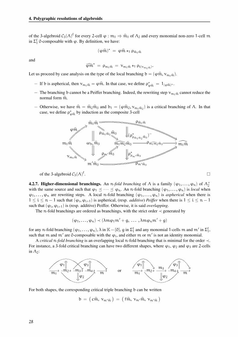
4. Polygraphic resolutions of algebroids
of the 3-algebroid C3(Λ)ℓ
for every 2-cell ϕ : m1 ⇒ m1 of Λ2 and every monomial non-zero 1-cell m
in Σℓ1 0-composable with ϕ. By definition, we have:
(ϕm)∗ = ϕm ⋆1 ρm1m
and
ϕm∗= ρm1m = νm1m ⋆1 ρt(νm1m
).
Let us proceed by case analysis on the type of the local branching b = (ϕm, νm1m).
− If b is aspherical, then νm1m = ϕm. In that case, we define ρ∗ϕm = 1(ϕm)∗ .
− The branching b cannot be a Peiffer branching. Indeed, the rewriting step νm1m cannot reduce the
normal form m.
− Otherwise, we have m = m2m3 and b1 = (ϕm2, νm1m2) is a critical branching of Λ. In that
case, we define ρ∗ϕm by induction as the composite 3-cell
m1m
ρm1m2m3
IIIIIIIIII
�.IIIIIIII
ωb1m3
���
ρm1m
�0m1m
ϕm.B
νm1m �0
m1m2m3ρm1m2m3
%9 m1m
m ′m3
ρm ′m3uuuuuuuuuu
0Duuuuuuuu
ρm ′m3
.B
(ρ∗ρm1m2m3
)−���
ρ∗ρm ′m3���
of the 3-algebroid C3(Λ)ℓ.
4.2.7. Higher-dimensional branchings. An n-fold branching of Λ is a family (ϕ1, . . . , ϕn) of Λ+2
with the same source and such that ϕ1 � · · · � ϕn. An n-fold branching (ϕ1, . . . , ϕn) is local when
ϕ1, . . . , ϕn are rewriting steps. A local n-fold branching (ϕ1, . . . , ϕn) is aspherical when there is
1 ≤ i ≤ n − 1 such that (ϕi, ϕi+1) is aspherical, (resp. additive) Peiffer when there is 1 ≤ i ≤ n − 1
such that (ϕi, ϕi+1) is (resp. additive) Peiffer. Otherwise, it is said overlapping.
The n-fold branchings are ordered as branchings, with the strict order ≺ generated by
(ϕ1, . . . , ϕn) ≺ (λmϕ1m′ + g, . . . , λmϕnm
′ + g)
for any n-fold branching (ϕ1, . . . , ϕn), λ in K− {0}, g in Σℓ1 and any monomial 1-cellsm andm ′ in Σℓ1,
such thatm andm ′ are 0-composable with the ϕi, and eitherm orm ′ is not an identity monomial.
A critical n-fold branching is an overlapping local n-fold branching that is minimal for the order ≺.
For instance, a 3-fold critical branching can have two different shapes, where ϕ1, ϕ2 and ϕ3 are 2-cells
in Λ2:
m1
//��
m2 //BBm3 //
��m4 //
m//
ϕ1
EY
ϕ2��
ϕ3
EY
orm1
//��
m2 //BB
m3// m4 //
��
m//
ϕ1
EY
ϕ2��
ϕ3
EY
For both shapes, the corresponding critical triple branching b can be written
b =(cm, νm ′m
)=
(fm, νm ′m, νm ′m
)
28
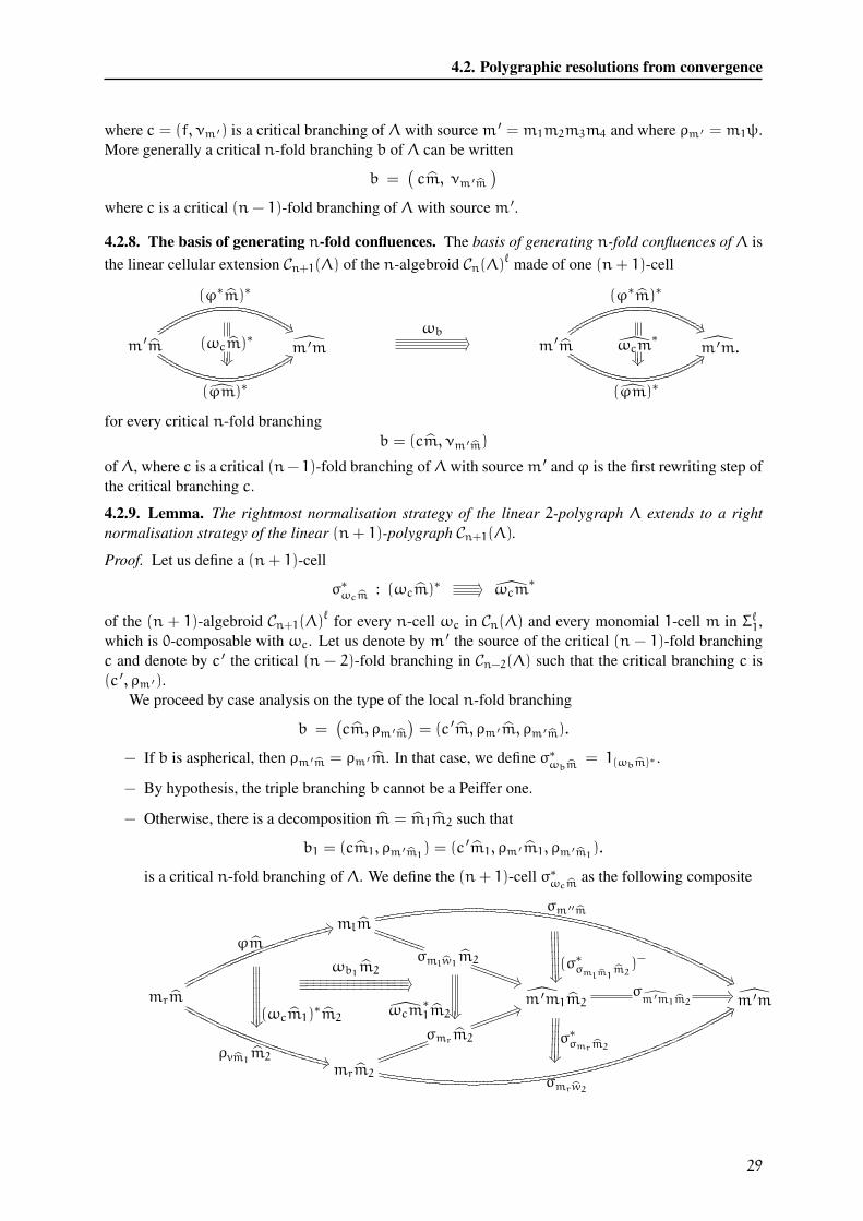
4.2. Polygraphic resolutions from convergence
where c = (f, νm ′) is a critical branching of Λ with sourcem ′ = m1m2m3m4 and where ρm ′ = m1ψ.
More generally a critical n-fold branching b of Λ can be written
b =(cm, νm ′m
)
where c is a critical (n− 1)-fold branching of Λ with sourcem ′.
4.2.8. The basis of generating n-fold confluences. The basis of generating n-fold confluences of Λ is
the linear cellular extension Cn+1(Λ) of the n-algebroid Cn(Λ)ℓ
made of one (n+ 1)-cell
m ′m
(ϕ∗m)∗
�.
(ϕm)∗
0Dm′m
ωb�? m ′m
(ϕ∗m)∗
�.
(ϕm)∗
0Dm′m.(ωcm)∗
���ωcm
∗
���
for every critical n-fold branching
b = (cm, νm ′m)
of Λ, where c is a critical (n− 1)-fold branching of Λ with sourcem ′ and ϕ is the first rewriting step of
the critical branching c.
4.2.9. Lemma. The rightmost normalisation strategy of the linear 2-polygraph Λ extends to a right
normalisation strategy of the linear (n+ 1)-polygraph Cn+1(Λ).
Proof. Let us define a (n+ 1)-cell
σ∗ωcm: (ωcm)∗ �? ωcm
∗
of the (n + 1)-algebroid Cn+1(Λ)ℓ
for every n-cell ωc in Cn(Λ) and every monomial 1-cell m in Σℓ1,
which is 0-composable with ωc. Let us denote by m ′ the source of the critical (n − 1)-fold branching
c and denote by c ′ the critical (n − 2)-fold branching in Cn−2(Λ) such that the critical branching c is
(c ′, ρm ′).
We proceed by case analysis on the type of the local n-fold branching
b =(cm, ρm ′m
)= (c ′m, ρm ′m, ρm ′m).
− If b is aspherical, then ρm ′m = ρm ′m. In that case, we define σ∗ωbm= 1(ωbm)∗ .
− By hypothesis, the triple branching b cannot be a Peiffer one.
− Otherwise, there is a decomposition m = m1m2 such that
b1 = (cm1, ρm ′m1) = (c ′m1, ρm ′m1, ρm ′m1
).
is a critical n-fold branching of Λ. We define the (n+ 1)-cell σ∗ωcmas the following composite
mlm
σmlw1m2
SSSSSSSSSSSSSSSS
�3SSSSSSSSSSSSSS
σm ′′m
�/mrm
ϕm
)=
ρvm1m2 !5
m ′m1m2σm ′m1m2
%9m ′m
mrm2
σmrm2kkkkkkkkkkkkkkkk
+?kkkkkkkkkkkkkk
σmrw2
/C
(σ∗σmlm1m2
)− ��
σ∗σmrm2
��� ������
������
������
(ωcm1)∗m2���
��������
��������
��������
ωcm∗
1m2���
ωb1m2�?________________ ________________ ________________ ________________
29
5. Free resolutions of algebroids
in the (n+ 1)-algebroid Cn+1(Λ)ℓ, where ϕ is the first reducing step of the critical n-fold branch-
ing c.
We apply Proposition 4.1.8 to extend the family of (n+1)-cells we have defined to a right normalisation
strategy of the linear (n+ 1)-polygraph Cn+1(Σ).
As a conclusion of this construction, we get that the (n+ 1)-polygraph Cn+1(Λ) is acyclic.
4.2.10. Theorem. Any convergent linear 2-polygraph Λ extends to a Tietze-equivalent acyclic linear
∞-polygraph C∞(Λ), whose n-cells, for n ≥ 3, are indexed by the critical (n− 1)-fold branchings.
5. FREE RESOLUTIONS OF ALGEBROIDS
5.1. Free modules resolution from polygraphic resolutions
5.1.1. Modules and bimodules over an algebroid. Given an algebroid A, a (left) A-module is a linear
functorM : A→ Vect. Denote by Ao the opposite algebroid and denote by Ae the enveloping algebroid
define by Ao⊗A, where ⊗ denotes the natural tensor product on algebroids. We define a right A-module
(resp. A-bimodule) as a Ao-module (resp. Ae-module). The A-modules and their natural transformations
form an Abelian category denoted by Mod(A). The free A-modules are the coproducts of representable
functors A(p,−), where p is a 0-cell of A.
If M is an A-module and x an element in M(p), for p in A0, we simply say that x is an element of
M. For u in A(p, q), we will denote ux for M(u)(x). If F :M → N is a morphism of A-modules, we
denote F(x) for F(p)(x).
5.1.2. A free bimodules resolution. Let A be an algebroid and let Λ be a linear ∞-polygraph whose
underlying 2-polygraph is a presentation of A. We suppose that a basis Σ is fixed for Λ. We denote by
Ae[Λk] the free A-bimodule on Λk, defined by
Ae[Λk] =⊕
f∈Σk
A(−, s0(f))⊗ A(t0(f),−) ≃⊕
f∈Σk
Ae((s0(f), t0(f)), (−,−)).
Explicitly, for 0-cells p and q in A, the value of the functor Ae[Λk] in (p, q) is the space given by the
linear combinations of u ⊗ f ⊗ v, denoted by u[f]v, where u and v are 1-cells in A and f is a k-cell in
Σk, such that the 0-composition us1(f)v is defined in A(p, q). When k = 0, a triple u[p0]v, such that
t0(u) = p0 = s0(v) will be denoted by u⊗ v.The mapping of every 1-cell x in Σ1 to the element [x] in Ae[Λ1](s0(x), t0(x)) is uniquely extended
on a derivation, denoted by [·], from Λℓ1 with values in the A-bimodule Ae[Λ1], sending a 1-cell u on the
element [u] in Ae[Λ1](s0(u), t0(u)), defined by induction on the weight of u by
[1p] = 0, [uv] = [u]v+ u[v],
for any 0-cell p of A and any 0-composable 1-cells u and v in Σℓ1.
We extend the bracket notation to A-bimodules Ae[Λk], for 1 < k ≤ n as follows. The mapping
of every k-cell f of Σk to the element [f] in Ae[Λk](s0(f), t0(f)) is extended to any k-cell f of Λℓk by
induction on the size of f. For any (k− 1)-cell u, any k-cells f and g and scalar λ, we set
[1u] = 0, [f+ g] = [f] + [g], [f ⋆0 g] = [f]g+ f[g], [λf] = λ[f].
Note that using relations in 2.1.6, we deduce that
[f−] = −[f], [f ⋆l g] = [f] + [g],
30
5.1. Free modules resolution from polygraphic resolutions
for any l-composable k-cells f and g and 1 ≤ l ≤ k− 1. The bracket map [·] is well-defined, because it
is compatible with the exchange relations, for every 0 ≤ l1 < l2 ≤ k:
[(f ⋆l1 g) ⋆l2 (h ⋆l1 k)] = [(f ⋆l2 h) ⋆l1 (g ⋆l2 k)] =
{[f]g+ f[g] + [h]k+ h[k] if l1 = 0
[f] + [g] + [h] + [k] otherwise.
To the linear∞-polygraph Λ, we associate a complex of A-bimodules
0←− Aµoo Ae[Λ0]
δ0oo Ae[Λ1]←− . . . ←− Ae[Λk]
δkoo Ae[Λk+1]←− . . .
where the boundary maps are the functors defined as follows. The maps µ is defined by µ(u⊗ v) = uv,
for any 0-composable pair pu
// p0v// q in A. For any triple u[x]v in Ae[Λ1], we define
δ0(u[x]v) = u⊗ xv− ux⊗ v.
For k ≥ 1, for any triple u[f]v in Ae[Λk+1], we define
δk(u[f]v) = u[sk(f)]v− u[tk(f)]v.
By induction, we prove that δ0([w]) = 1 ⊗w −w ⊗ 1, for any 1-cell w in Λℓ1. We have µδ0 = 0. For
any k-cell f, with k ≥ 2, we have
δk−1δk[f] = [sk−1sk(f)] + [tk−1sk(f)] − [sk−1tk(f)] − [tk−1tk(f)].
It follows from the globular relations that δk−1δk = 0. Moreover, the acyclicity of the polygraph induces
the acyclic of the complex as shown by following result.
5.1.3. Theorem. If Λ is a (finite) ω-concentrated polygraphic resolution of an algebroid A, then the
complex Ae[Λ] is a (finite)ω-concentrated free resolution of the A-bimodule A.
This bimodule resolution can be used to compute Hochschild homology, as in [8, Section 5].
Proof. Suppose thatΛ is a polygraphic resolution of the algebroid A. Fix a section · ofΛ. The polygraph
Λ being acyclic, by Proposition 4.1.9, it admits a right normalisation strategy σ. The strategy σ induces
a contracting homotopy ι for the complex Ae[Λ] constructed as follows. We define the maps
ι0 : A→ Ae[Λ0], ι1 : Ae[Λ0]→ Ae[Λ1]
by
ι0(u) = u⊗ 1 and ι1(u⊗ v) = u[v].
We have ι0µ(u⊗ v) = uv⊗ 1 and δ0ι1(u⊗ v) = u⊗ v−uv⊗ 1, thus ι0µ+ δ0ι1 = IdAe[Λ0]. For k ≥ 2,we define the map
ιk : Ae[Λk−1]→ Ae[Λk]
by
ιk(u[f]v) = u[σfv].
We prove by induction on the size that for any (k − 1)-cell f in Λℓk−1, ιk(u[f]v) = u[σfv]. If f is an
identity map 1w on some (k− 2)-cell w, we have
ιk(u[1w]v) = 0 = u[σ1wv].
31
5. Free resolutions of algebroids
Suppose that f is a 0-composite of non-identity cells of size lower than the size of f: f = f1 ⋆0 f2, by
induction we have
ιk(u[f1 ⋆0 f2]v) = ιk(u[f1]f2v) + ιk(uf1[f2]v),
= u[σf1
f2v
] + uf1[σf2v]
= u([σf1
f2v
] + f1[σf2v])
= u([σf1
f2v
] + s1(f1)[σf2v])
= u[σf1f2v].
Suppose that f is a l-composite of non-identity cells of size lower than the size of f: f = f1 ⋆l f2, with
l ≥ 1, by induction we have
ιk(u[f1 ⋆l f2]v) = ιk(u[f1]v) + ιk(u[f2]v),
= u[σf1v] + u[σf2v]
= u([σf1v] + [σf2v]
)
= u[σf1v ⋆l σf2v]
= u[σ(f1⋆lf2)v].
We have ι1δ0(u[x]v) = u[xv] − ux[v] and
δ1ι2(u[x]v) = δ1(u[σxv]) = u[xv] − u[xv] = ux[v] + u[x]v− u[xv].
Thus ι1δ0 + δ1ι2 = IdAe[Λ1]. Let k ≥ 2 and let u[f]v in Ae[Λk], we have
δkιk+1(u[f]v) = δk(u[σfv]) = u[fv] − u[σsk−1(f)v ⋆k−1 σ−tk−1(f)v
],
= u[fv] − u[σsk−1(f)v] + u[σ−tk−1(f)v
],
= ιk(u[sk−1(f)]v) − ιk(u[tk−1(f)]v),
= ιkδk−1(u[f]v).
Thus ιkδk−1 + δkιk+1 = IdAe[Λk].
5.1.4. A free right modules resolution. Recall that A(0)k (p, p) = K for any 0-cell p in Σ0 and any k ∈
N, where the 1-dimensional space is generated by the identity k-cell. Also, recall that A(0)(p, q) = {0}
for distinct 0-cells p and q in Σ0.
When Λ is a polygraphic resolution of A, the complex of A-modules A(0) ⊗A Ae[Λ], whose bound-
ary map defined by δk = 1 ⊗ δk, is a resolution of A(0) as a right A-module. However, in general
this resolution is not homogeneous even if the polygraphic resolution is homogeneous. We construct a
homogeneous resolution of A(0) in the category of right A-modules using a homogeneous polygraphic
resolution as follows.
Let A be an algebroid and let Λ be a linear∞-polygraph whose underlying 2-polygraph is a presen-
tation of A. We suppose that a basis Σ is fixed for Λ. For any k ≥ 0, denote by A[Λk] the free right
A-module generated by Λk, defined by
A[Λk] =⊕
f∈Σk
A(t0(f),−).
The value of the functor A[Λk] in a 0-cell q is the space given by the linear combinations of f ⊗ u,
denoted by [f]u, where u is 1-cell in A and f is a k-cell in Σk, such that the 0-composition s1(f)u is
defined in A(s0(f), q). The elements of A[Λ0] are identified to the 1-cells of A.
32

5.1. Free modules resolution from polygraphic resolutions
The mapping of every 1-cell x in Σ1 to the element [x] in A[Λ1](s0(x), t0(x)) is extended to the
algebroid Σℓ1 by setting
[1p] = 0, [xy] = [x]y,
for any 0-cell p and 0-composable 1-cells x and y in Σℓ1. The mapping of every k-cell f of Σk to the
element [f] in A[Λk](t0(f)) is extended to any k-cell f of Λℓk by induction on the size of f. For any
(k− 1)-cell u, any k-cells f and g and scalar λ, we set
[1u] = 0, [f+ g] = [f] + [g], [f ⋆0 g] = [f]g, [λf] = λ[f].
Note that using relations in 2.1.6, we deduce that
[f−] = −[f], [f ⋆l g] = [f] + [g],
for any k-cells f and g and 1 ≤ l ≤ n− 1. The bracket map [·] is well-defined, because it is compatible
with the exchange relations, for every 0 ≤ l1 < l2 ≤ k:
[(f ⋆l1 g) ⋆l2 (h ⋆l1 k)] = [(f ⋆l2 h) ⋆l1 (g ⋆l2 k)] = [f] + [g] + [h] + [k],
and
[(f ⋆0 g) ⋆l (h ⋆0 k)] = [f ⋆0 g] + [h ⋆0 k] = [f]u+ [h]u,
where u denotes g = k. On the other hand, we have
[(f ⋆l h) ⋆0 (g ⋆l k)] = [f ⋆l h]g ⋆1 k = [f ⋆l h]u = [f]u+ [h]u.
To the linear∞-polygraph Λ, we associate a complex of right A-modules
0←− A(0) εoo A[Λ0]
δ0oo A[Λ1]←− . . . ←− A[Λk]
δkoo A[Λk+1]←− . . .
where the boundary maps are the functors defined as follows. The map ε is the augmentation defined by
ε(u) = u if u is an identity and ε(u) = 0 in the other cases. For any [x]u in A[Λ1], we define
δ0([x]u) = xu.
For k ≥ 1, for any [f]u in A[Λk+1], we define
δk([f]u) = [sk(f)]u− [tk(f)]u.
By induction, we prove that δ0([u]) = u, for any 1-cell u in Λℓ1. We have εδ0 = 0 and for any k-cell f,
with k ≥ 2, we have
δk−1δk[f] = [sk−1sk(f)] + [tk−1sk(f)] − [sk−1tk(f)] − [tk−1tk(f)].
It follows from the globular relations that δk−1δk = 0. As for bimodules, if the polygraph is acyclic, then
the complex is acyclic.
5.1.5. Theorem. If Λ is a (finite) ω-concentrated polygraphic resolution of an algebroid A, then the
complex A[Λ] is a (finite)ω-concentrated free resolution of the trivial right A-module A(0).
Proof. Suppose that Λ is a polygraphic resolution of the algebroid A, with a fixed section · of Λ. The
polygraph Λ admits a right normalisation strategy σ from which we construct a contracting homotopy ι
for the complex Ae[Λ] as in Theorem 5.1.3. We define the maps
ι0 : A(0) → A[Λ0], ι1 : A[Λ0]→ A[Λ1]
33

5. Free resolutions of algebroids
by
ι0(1q) = 1q and ι1(u) = [u].
We have ι0ε(1q) = 1q and δ0ι1(1q) = 0. And, if u is not an identity, we have ι0ε(u) = 0 and
δ0ι1(u) = u. It follows that ι0ε+ δ0ι1 = IdA[Λ0]. For k ≥ 2, we define the map
ιk : A[Λk−1]→ A[Λk]
by
ιk([f]u) = [σfu].
As in the proof of Theorem 5.1.3, we prove by induction on the size of f, that for any (k − 1)-cell f in
Λℓk−1 that ιk([f]u) = [σfu]. For any x[u] in A[Λ1], we have
(ι1δ0 + δ1ι2)([x]u) = ι1(xu) + δ1([σxu]),
= [xu] + [s1(σxu)] − [t1(σxu)],
= [xu] = [x]u.
Thus ι1δ0 + δ1ι2 = IdA[Λ1]. Let k ≥ 2 and let [f]u in A[Λk], we have
δkιk+1([f]u) = δk([σfu]) = [fu] − [σsk−1(f)u ⋆k−1 σ−tk−1(f)u
],
= [fu] − [σsk−1(f)u] + [σ−tk−1(f)u
],
= ιk([sk−1(f)]u) − ιk([tk−1(f)]u),
= ιkδk−1([f]u).
Thus ιkδk−1 + δkιk+1 = IdA[Λk].
This resolution and the associated theorem for right A-modules can be adapted to the setting of left
A-modules.
5.2. Finiteness properties
Throughout this section, n ≥ 1 denotes a natural number.
5.2.1. Algebroids of finite derivation type. An algebroid is of finite n-derivation type, FDTn for short,
when it admits a finite partial polygraphic resolution of length n. An algebroid is of finite∞-derivation
type, FDT∞ for short, when it admits a finite polygraphic resolution, i.e., when it is FDTn for every
n ≥ 1.In particular, an algebroid is FDT1 when it is finitely generated, it is FDT2 when it is finitely pre-
sented. The property FDT3 corresponds to the finite derivation type condition originally defined by
Squier for monoids in [31]. The property FDTn, for n ≥ 3 for higher-dimension categories were intro-
duced in [20, 2.3.6.]. Let us note that for any n ≥ 1, the property FDTn+1 implies the property FDTn.
By Proposition 4.1.9, a linear p-polygraph is acyclic if and only if it is right normalising. It follows
the following result.
5.2.2. Proposition. Let n ≥ 1 be a natural number. An algebroid A is FDTn if and only if there exists
a finite right normalising linear n-polygraph presenting A.
In Section 4.2, we construct a polygraphic resolution for an algebroid from a convergent presentation.
By Theorem 4.2.10, we have
5.2.3. Proposition. An algebroid with a finite convergent presentation is FDT∞.
34
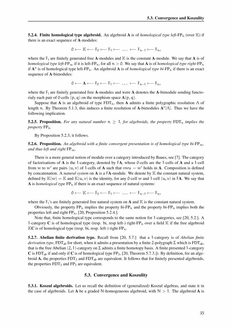
5.3. Convergence and Koszulity
5.2.4. Finite homological type algebroid. An algebroid A is of homological type left-FPn (over K) if
there is an exact sequence of A-modules:
0←− K←− F0 ←− F1 ←− . . . ←− Fn−1 ←− Fn,
where the Fi are finitely generated free A-modules and K is the constant A-module. We say that A is of
homological type left-FP∞ if it is left-FPn, for all n > 0. We say that A is of homological type right-FPnif Ao is of homological type left-FPn. An algebroid A is of homological type bi-FPn if there is an exact
sequence of A-bimodules:
0←− A←− F0 ←− F1 ←− . . . ←− Fn−1 ←− Fn,
where the Fi are finitely generated free A-modules and were A denotes the A-bimodule sending functo-
rialy each pair of 0-cells (p, q) on the morphism space A(p, q).
Suppose that A is an algebroid of type FDTn, then A admits a finite polygraphic resolution Λ of
length n. By Theorem 5.1.3, this induces a finite resolution of A-bimodules Ae[Λ]. Thus we have the
following implication.
5.2.5. Proposition. For any natural number n ≥ 1, for algebroids, the property FDTn implies the
property FPn.
By Proposition 5.2.3, it follows.
5.2.6. Proposition. An algebroid with a finite convergent presentation is of homological type bi-FP∞,
and thus left and right FP∞.
There is a more general notion of module over a category introduced by Baues, see [7]. The category
of factorisations of A is the 1-category, denoted by FA, whose 0-cells are the 1-cells of A and a 1-cell
from w to w ′ are pairs (u, v) of 1-cells of A such that vwu = w ′ holds in A. Composition is defined
by concatenation. A natural system on A is a FA-module. We denote by K the constant natural system,
defined by K(w) = K and K(u, v) is the identity, for any 0-cell w and 1-cell (u, v) in FA. We say that
A is homological type FPn if there is an exact sequence of natural systems:
0←− K←− F0 ←− F1 ←− . . . ←− Fn−1 ←− Fn,
where the Fi’s are finitely generated free natural system on A and K is the constant natural system.
Obviously, the property FPn implies the property bi-FPn and the property bi-FPn implies both the
properties left and right FPn, [20, Proposition 5.2.4.].
Note that, finite homological type corresponds to the same notion for 1-categories, see [20, 5.2.]. A
1-category C is of homological type (resp. bi, resp left-) right-FPn over a field K if the free algebroid
KC is of homological type (resp. bi, resp. left-) right-FPn.
5.2.7. Abelian finite derivation type. Recall from [20, 5.7.] that a 1-category is of Abelian finite
derivation type, FDTab for short, when it admits a presentation by a finite 2-polygraph Σ which is FDTab,
that is the free Abelian (2, 1)-category on Σ admits a finite homotopy basis. A finite presented 1-category
C is FDTab if and only if C is of homological type FP3, [20, Theorem 5.7.3.]). By definition, for an alge-
broid A, the properties FDT3 and FDTab are equivalent. It follows that for finitely presented algebroids,
the properties FDT3 and FP3 are equivalent.
5.3. Convergence and Koszulity
5.3.1. Koszul algebroids. Let us recall the definition of (generalized) Koszul algebras, and state it in
the case of algebroids. Let A be a graded N-homogeneous algebroid, with N > 1. The algebroid A is
35
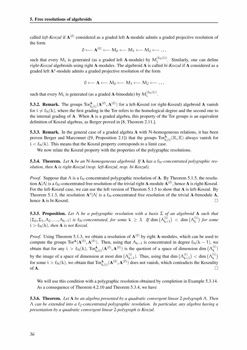
5. Free resolutions of algebroids
called left-Koszul if A(0) considered as a graded left A-module admits a graded projective resolution of
the form
0←− A(0) ←−M0 ←−M1 ←−M2 ←− . . .
such that every Mi is generated (as a graded left A-module) by M(ℓN(i))i . Similarly, one can define
right-Koszul algebroids using right A-modules. The algebroid A is called bi-Koszul if A considered as a
graded left Ae-module admits a graded projective resolution of the form
0←− A←−M0 ←−M1 ←−M2 ←− . . .
such that everyMi is generated (as a graded A-bimodule) byM(ℓN(i))i .
5.3.2. Remark. The groups TorAk,(i)(A
(0),A(0)) for a left-Koszul (or right-Koszul) algebroid A vanish
for i 6= ℓN(k), where the first grading in the Tor refers to the homological degree and the second one to
the internal grading of A. When A is a graded algebra, this property of the Tor groups is an equivalent
definition of Koszul algebras, as Berger proved in [8, Theorem 2.11.].
5.3.3. Remark. In the general case of a graded algebra A with N-homogeneous relations, it has been
proven Berger and Marconnet ([9, Proposition 2.1]) that the groups TorAk,(i)(K,K) always vanish for
i < ℓN(k). This means that the Koszul property corresponds to a limit case.
We now relate the Koszul property with the properties of the polygraphic resolutions.
5.3.4. Theorem. Let A be an N-homogeneous algebroid. If A has a ℓN-concentrated polygraphic res-
olution, then A is right-Koszul (resp. left-Koszul, resp. bi-Koszul).
Proof. Suppose that Λ is a ℓN-concentrated polygraphic resolution of A. By Theorem 5.1.5, the resolu-
tion A[Λ] is a ℓN-concentrated free resolution of the trivial right A-module A(0), hence A is right-Koszul.
For the left-Koszul case, we can use the left version of Theorem 5.1.5 to show that A is left-Koszul. By
Theorem 5.1.3, the resolution Ae[Λ] is a ℓN-concentrated free resolution of the trivial A-bimodule A,
hence A is bi-Koszul.
5.3.5. Proposition. Let Λ be a polygraphic resolution with a basis Σ of an algebroid A such that
(Σ0, Σ1, Λ2 . . . , Λk−1) is ℓN-concentrated, for some k ≥ 3. If dim(Λ
(i)k+1
)< dim
(Λ
(i)k
)for some
i > ℓN(k), then A is not Koszul.
Proof. Using Theorem 5.1.3, we obtain a resolution of A(0) by right A-modules, which can be used to
compute the groups TorA(A(0),A(0)). Then, using that Λk−1 is concentrated in degree ℓN(k − 1), we
obtain that for any i > ℓN(k), TorAk,(i)(A
(0),A(0)) is the quotient of a space of dimension dim(Λ
(i)k )
by the image of a space of dimension at most dim(Λ
(i)k+1). Thus, using that dim
(Λ
(i)k+1
)< dim
(Λ
(i)k
)
for some i > ℓN(k), we obtain that TorAk,(i)(A
(0),A(0)) does not vanish, which contradicts the Koszulity
of A.
We will use this condition with a polygraphic resolution obtained by completion in Example 5.3.14.
As a consequence of Theorem 4.2.10 and Theorem 5.3.4, we have
5.3.6. Theorem. Let A be an algebra presented by a quadratic convergent linear 2-polygraph Λ. Then
Λ can be extended into a ℓ2-concentrated polygraphic resolution. In particular, any algebra having a
presentation by a quadratic convergent linear 2-polygraph is Koszul.
36
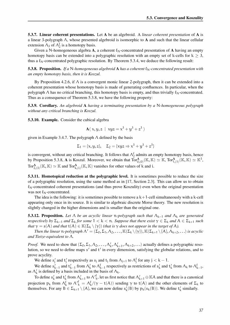
5.3. Convergence and Koszulity
5.3.7. Linear coherent presentations. Let A be an algebroid. A linear coherent presentation of A is
a linear 3-polygraph Λ, whose presented algebroid is isomorphic to A and such that the linear cellular
extension Λ3 of Λℓ2 is a homotopy basis.
Given a N-homogeneous algebra A, a coherent ℓN-concentrated presentation of A having an empty
homotopy basis can be extended into a polygraphic resolution with an empty set of k-cells for k ≥ 3,
thus a ℓN-concentrated polygraphic resolution. By Theorem 5.3.4, we deduce the following result:
5.3.8. Proposition. If aN-homogeneous algebroid A has a coherent ℓN-concentrated presentation with
an empty homotopy basis, then it is Koszul.
By Proposition 4.2.6, if Λ is a convergent monic linear 2-polygraph, then it can be extended into a
coherent presentation whose homotopy basis is made of generating confluences. In particular, when the
polygraph Λ has no critical branching, this homotopy basis is empty, and thus trivially ℓN-concentrated.
Thus as a consequence of Theorem 5.3.8, we have the following property:
5.3.9. Corollary. An algebroid A having a terminating presentation by a N-homogeneous polygraph
without any critical branching is Koszul.
5.3.10. Example. Consider the cubical algebra
A〈 x, y, z | xyz = x3 + y3 + z3 〉
given in Example 3.4.7. The polygraph Λ defined by the basis
Σ1 = {x, y, z}, Σ2 = {xyz⇒ x3 + y3 + z3}
is convergent, without any critical branching. It follows that Λℓ2 admits an empty homotopy basis, hence
by Proposition 5.3.8, A is Koszul. Moreover, we obtain that TorA0,(0)(K,K) ≃ K, TorA
1,(1)(K,K) ≃ K3,
TorA2,(3)(K,K) ≃ K and TorA
k,(i)(K,K) vanishes for other values of k and i.
5.3.11. Homotopical reduction at the polygraphic level. It is sometimes possible to reduce the size
of a polygraphic resolution, using the same method as in [17, Section 2.3]. This can allow us to obtain
ℓN-concentrated coherent presentations (and thus prove Koszulity) even when the original presentation
was not ℓN-concentrated.
The idea is the following: it is sometimes possible to remove a k+1-cell simultaneously with a k-cell
appearing only once in its source. It is similar to algebraic discrete Morse theory. The new resolution is
slightly changed in the higher dimensions and is smaller than the original one.
5.3.12. Proposition. Let Λ be an acyclic linear n-polygraph such that Λk−1 and Λk are generated
respectively by Σk−1 and Σk for some 1 < k < n. Suppose that there exist γ ∈ Σk and A ∈ Σk+1 such
that γ = s(A) and that t(A) ∈ K(Σk \ {γ}) (that is γ does not appear in the target of A).
Then the linear n-polygraph Λ ′ = (Σ0, Σ1, Λ2, . . . ,K(Σk \ {γ}),K(Σk+1 \ {A}, Λk+2, . . .) is acyclic
and Tietze-equivalent to Λ.
Proof. We need to show that (Σ0, Σ1, Λ2, . . . , Λ′k, Λ
′k+1, Λk+2, . . .) actually defines a polygraphic reso-
lution, so we need to define maps s ′ and t ′ in every dimension, satisfying the globular relations, and to
prove acyclity.
We define s ′j and t ′j respectively as sj and tj from Λj+1 to Λℓj for any j < k− 1.
We define s ′k−1 and t ′k−1 from Λ ′k to Λℓk−1 respectively as restrictions of s ′k and t ′k from Λk to Λℓk−1,
as Λ ′k is defined by a basis included in the basis of Λk.
To define s ′k and t ′k fromΛ ′k+1 toΛ ′ℓ
k, let us first notice thatΛ ′k+1⊕KA and that there is a canonical
projection pk from Λℓk to Λ ′ℓk = Λℓk/(γ − t(A)) sending γ to t(A) and the other elements of Σk to
themselves. For any B ∈ Σk+1 \ {A}, we can now define s ′k(B) by pk(sk(B)). We define t ′k similarly.
37

5. Free resolutions of algebroids
Note that Λ ′ℓj = Λ
ℓj/(A,γ − t(A)) for any j > k. We define s ′j = pj ◦ sj and t ′j = pj ◦ tj where pj
denotes the projection Λℓj → Λ ′ℓj .
The globular relations still hold.
To prove the acyclicity of Λ ′, note first that Λ and Λ ′ coincide in dimensions smaller than k. Thus
we only have to prove acyclicity in dimension j when j ≥ k.
The space of j-spheres of Λ ′ is a quotient of the space of j-spheres of Λ. Given a j-sphere S ′ of Λ ′,
we take a j-sphere S of Λ lifting S ′. There exists a j+ 1-cell B of Λℓj+1 such that S is the boundary of B.
Then pj+1(B) is a j+ 1-cell of Λ ′ℓj+1 whose boundary is S ′.
5.3.13. Example. Consider the following quadratic algebra
A〈 x, y, z | x2 + yz = 0, x2 + azy = 0 〉,
with a 6= 0 and a 6= 1, see [29, Section 4.3]. Consider the linear 2-polygraph Λ with Σ1 = {x, y, z} and
Λ2 is generated by the following quadratic 2-cells:
yz α %9 −x2 zyβ %9 bx2
where b = −1/a. There are two cubical critical branchings
byx2
yzy
yβ (<
αz "6−x2y
bx2z
zyz
βz (<
zα "6−zx2
We complete the linear polygraph Λ into a convergent linear polygraph, denoted by Λ, by adding the
cubical rules
yx2γ %9 ax2y zx2
δ %9 −bx2z
The linear polygraph Λ has the following four confluent critical branchings:
byx2
bγ
��
yzy
yβ (<
αy "6−x2y
A1�y ��������
��������
��������bx2z
zyz
βz (<
zα "6−zx2
−δ
EY
B1
9Rf99999999
99999999
99999999
bx4
zyx2
βx2 (<
zγ !5
x2zy
x2βbv
azx2y aδy
0DC1
S_s SSSSSSSSSSS
SSSSSSSSSSS
SSSSSSSSSSS
−x4
yzx2
αx2 (<
yδ !5
x2yz
x2αcw
−byx2z −bγz
/CD1
U`t UUUUUUUUUUUUU
UUUUUUUUUUUUU
UUUUUUUUUUUUU
By Proposition 4.2.6, these four 3-cells extend the polygraph Λ into a coherent presentation of the alge-
bra A.
Note that the 3-cells C1 andD1 are in weight 4, thus the linear 3-polygraph Λ is not ℓ2-concentrated.
We now investigate higher critical branchings, to understand the polygraphic resolution of A. There are
four critical triple branchings, whose 1-sources are respectively
yzyz, yzyx2, zyzy, zyzx2.
38
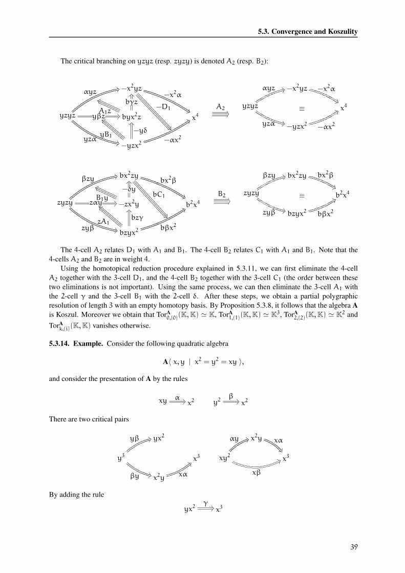
5.3. Convergence and Koszulity
The critical branching on yzyz (resp. zyzy) is denoted A2 (resp. B2):
−x2yz−x2α
�.yzyz
αyz(<
yβz %9
yzα "6
byx2z
bγz
EY
x4
−yzx2
−yδ
EY
−αx2
0DA1z
P^r PPPPPPP
PPPPPPPPPPPPPP
yB1
DWkDDDDDDDDD
DDDDDDDDD
DDDDDDDDD
−D1
=�(===============
===============
===============
A2�?
−x2yz −x2α
�.yzyz
αyz )=
yzα !5
x4
−yzx2 −αx2
0D≡
bx2zybx2β
�.zyzy
βzy(<
zαy %9
zyβ "6
−zx2y
−δy
EY
b2x4
bzyx2
bzγ
EY
bβx2
0D
B1y
P]q PPPPPPP
PPPPPPPPPPPPPP
zA1
DWkDDDDDDDDD
DDDDDDDDD
DDDDDDDDD
bC1
<�(<<<<<<<<<<<<<<<
<<<<<<<<<<<<<<<
<<<<<<<<<<<<<<<
B2�?
bx2zy bx2β
�.zyzy
βzy )=
zyβ !5
b2x4
bzyx2 bβx2
0D≡
The 4-cell A2 relates D1 with A1 and B1. The 4-cell B2 relates C1 with A1 and B1. Note that the
4-cells A2 and B2 are in weight 4.
Using the homotopical reduction procedure explained in 5.3.11, we can first eliminate the 4-cell
A2 together with the 3-cell D1, and the 4-cell B2 together with the 3-cell C1 (the order between these
two eliminations is not important). Using the same process, we can then eliminate the 3-cell A1 with
the 2-cell γ and the 3-cell B1 with the 2-cell δ. After these steps, we obtain a partial polygraphic
resolution of length 3 with an empty homotopy basis. By Proposition 5.3.8, it follows that the algebra A
is Koszul. Moreover we obtain that TorA0,(0)(K,K) ≃ K, TorA
1,(1)(K,K) ≃ K3, TorA2,(2)(K,K) ≃ K2 and
TorAk,(i)(K,K) vanishes otherwise.
5.3.14. Example. Consider the following quadratic algebra
A〈 x, y | x2 = y2 = xy 〉,
and consider the presentation of A by the rules
xy α %9 x2 y2β %9 x2
There are two critical pairs
yx2
y3
yβ )=
βy !5
x3
x2y xα
3G
x2y xα
�&xy2
αy *>
xβ
.B x3
By adding the rule
yx2γ %9 x3
39
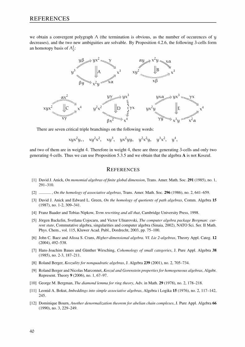
REFERENCES
we obtain a convergent polygraph Λ (the termination is obvious, as the number of occurences of y
decreases), and the two new ambiguities are solvable. By Proposition 4.2.6, the following 3-cells form
an homotopy basis of Λℓ2:
yx2 γ
�+y3
yβ )=
βy !5
x3
x2y xα
3GA���
x2y xα
�&xy2
αy *>
xβ
.B x3B���
xyx2
αx2
�,
xγ
2F x4C���
yx3
γx
��
y2x2
yγ (<
βx2#7x4
D�������
����
����
yx3 γx
�,yx2y
yxα (<
γy "6
x4
x3y x2α
2FE���
There are seven critical triple branchings on the following words:
xyx2y, , xy2x2, xy3, yx2yy, y2x2y, y3x2, y4,
and two of them are in weight 4. Therefore in weight 4, there are three generating 3-cells and only two
generating 4-cells. Thus we can use Proposition 5.3.5 and we obtain that the algebra A is not Koszul.
REFERENCES
[1] David J. Anick, On monomial algebras of finite global dimension, Trans. Amer. Math. Soc. 291 (1985), no. 1,
291–310.
[2] , On the homology of associative algebras, Trans. Amer. Math. Soc. 296 (1986), no. 2, 641–659.
[3] David J. Anick and Edward L. Green, On the homology of quotients of path algebras, Comm. Algebra 15
(1987), no. 1-2, 309–341.
[4] Franz Baader and Tobias Nipkow, Term rewriting and all that, Cambridge University Press, 1998.
[5] Jörgen Backelin, Svetlana Cojocaru, and Victor Ufnarovski, The computer algebra package Bergman: cur-
rent state, Commutative algebra, singularities and computer algebra (Sinaia, 2002), NATO Sci. Ser. II Math.
Phys. Chem., vol. 115, Kluwer Acad. Publ., Dordrecht, 2003, pp. 75–100.
[6] John C. Baez and Alissa S. Crans, Higher-dimensional algebra. VI. Lie 2-algebras, Theory Appl. Categ. 12
(2004), 492–538.
[7] Hans-Joachim Baues and Günther Wirsching, Cohomology of small categories, J. Pure Appl. Algebra 38
(1985), no. 2-3, 187–211.
[8] Roland Berger, Koszulity for nonquadratic algebras, J. Algebra 239 (2001), no. 2, 705–734.
[9] Roland Berger and Nicolas Marconnet, Koszul and Gorenstein properties for homogeneous algebras, Algebr.
Represent. Theory 9 (2006), no. 1, 67–97.
[10] George M. Bergman, The diamond lemma for ring theory, Adv. in Math. 29 (1978), no. 2, 178–218.
[11] Leonid A. Bokut, Imbeddings into simple associative algebras, Algebra i Logika 15 (1976), no. 2, 117–142,
245.
[12] Dominique Bourn, Another denormalization theorem for abelian chain complexes, J. Pure Appl. Algebra 66
(1990), no. 3, 229–249.
40
REFERENCES
[13] Bruno Buchberger, Ein Algorithmus zum Auffinden der Basiselemente des Restklassenringes nach einem
nulldimensionalen Polynomideal (An Algorithm for Finding the Basis Elements in the Residue Class Ring
Modulo a Zero Dimensional Polynomial Ideal), Ph.D. thesis, Mathematical Institute, University of Innsbruck,
Austria, 1965, English translation in J. of Symbolic Computation, Special Issue on Logic, Mathematics, and
Computer Science: Interactions. Vol. 41, Number 3-4, Pages 475–511, 2006.
[14] , History and basic features of the critical-pair/completion procedure, J. Symbolic Comput. 3 (1987),
no. 1-2, 3–38, Rewriting techniques and applications (Dijon, 1985).
[15] Albert Burroni, Higher-dimensional word problems with applications to equational logic, Theoret. Comput.
Sci. 115 (1993), no. 1, 43–62.
[16] Vladimir Dotsenko and Anton Khoroshkin, Gröbner bases for operads, Duke Math. J. 153 (2010), no. 2,
363–396.
[17] Stéphane Gaussent, Yves Guiraud, and Philippe Malbos, Coherent presentations of Artin monoids, Preprint,
arXiv:1203.5358v2, 2013.
[18] Edward Green and Rosa Q. Huang, Projective resolutions of straightening closed algebras generated by
minors, Adv. Math. 110 (1995), no. 2, 314–333.
[19] Edward L. Green, Noncommutative Gröbner bases, and projective resolutions, Computational methods for
representations of groups and algebras (Essen, 1997), Progr. Math., vol. 173, Birkhäuser, Basel, 1999, pp. 29–
60.
[20] Yves Guiraud and Philippe Malbos, Higher-dimensional normalisation strategies for acyclicity, Adv. Math.
231 (2012), no. 3-4, 2294–2351.
[21] , Polygraphs of finite derivation type, arXiv:1402.2587, 2014.
[22] Heisuke Hironaka, Resolution of singularities of an algebraic variety over a field of characteristic zero. I, II,
Ann. of Math. (2) 79 (1964), 109–203; ibid. (2) 79 (1964), 205–326.
[23] Yuji Kobayashi, Gröbner bases of associative algebras and the Hochschild cohomology, Trans. Amer. Math.
Soc. 357 (2005), no. 3, 1095–1124.
[24] Tom Leinster, Higher operads, higher categories, London Mathematical Society Lecture Note Series, vol.
298, Cambridge University Press, Cambridge, 2004.
[25] J.L. Loday and B. Vallette, Algebraic operads, Grundlehren Der Mathematischen Wissenschaften, vol. 346,
Springer, 2012.
[26] Barry Mitchell, Rings with several objects, Advances in Mathematics 8 (1972), 1–161.
[27] Teo Mora, An introduction to commutative and noncommutative Gröbner bases, Theoret. Comput. Sci. 134
(1994), no. 1, 131–173, Second International Colloquium on Words, Languages and Combinatorics (Kyoto,
1992).
[28] Maxwell Newman, On theories with a combinatorial definition of “equivalence”, Ann. of Math. (2) 43
(1942), no. 2, 223–243.
[29] Alexander Polishchuk and Leonid Positselski, Quadratic algebras, University Lecture Series, vol. 37, Amer-
ican Mathematical Society, Providence, RI, 2005.
[30] Anatoly Illarionovich Shirshov, Some algorithmic problems for Lie algebras., Sib. Mat. Zh. 3 (1962), 292–
296 (Russian).
[31] Craig Squier, Word problems and a homological finiteness condition for monoids, J. Pure Appl. Algebra 49
(1987), no. 1-2, 201–217.
[32] Ross Street, Limits indexed by category-valued 2-functors, J. Pure Appl. Algebra 8 (1976), no. 2, 149–181.
[33] , The algebra of oriented simplexes, J. Pure Appl. Algebra 49 (1987), no. 3, 283–335.
[34] Victor A. Ufnarovskij, Combinatorial and asymptotic methods in algebra, Algebra, VI, Encyclopaedia Math.
Sci., vol. 57, Springer, Berlin, 1995, pp. 1–196.
41
REFERENCES
YVES GUIRAUD
INRIA
Laboratoire Preuves, Programmes et Systèmes, CNRS UMR 7126,
Université Paris 7
Case 7014
75205 Paris Cedex 13.
ERIC HOFFBECK
Université Paris 13, Sorbonne Paris Cité
LAGA, CNRS UMR 7539
99 avenue Jean-Baptiste Clément
93430 Villetaneuse, France.
PHILIPPE MALBOS
Université de Lyon,
Institut Camille Jordan, CNRS UMR 5208
Université Claude Bernard Lyon 1
43, boulevard du 11 novembre 1918,
69622 Villeurbanne cedex, France.
42