linear models for regression - college of computinghic/8803-fall-09/slides/8803-09-lec03.pdf ·...

Introduction Preliminaries Linear Models Bayes Regress Model Comparison Summary References

Linear Models for Regression

Henrik I Christensen

Robotics & Intelligent Machines @ GTGeorgia Institute of Technology,

Atlanta, GA [email protected]

Henrik I Christensen (RIM@GT) Linear Regression 1 / 39

mailto:[email protected]


Outline

1 Introduction

2 Preliminaries

3 Linear Basis Function Models

4 Baysian Linear Regression

5 Baysian Model Comparison

6 Summary



Introduction

The objective of regression is to enable prediction of a value t basedon modelling over a dataset X .

Consider a set of D observations over a space

How can we generate estimates for the future?

Battery time?Time to completion?Position of doors?



Introduction (2)

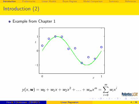
Example from Chapter 1

x

t

0 1

−1

0

1

y(x ,w) = w0 + w1x + w2x2 + . . . + wmxm =

m∑i=0

wixi



Introduction (3)

In general the functions could be beyond simple polynomials

The “components” are termed basis functions, i.e.

y(x ,w) =m∑

i=0

wiφi (x) = ~wT ~φ(x)



Outline

1 Introduction

2 Preliminaries




6 Summary



Loss Function

For optimization we need a penalty / loss function

L(t, y(x))

Expected loss is then

E [L] =

∫ ∫L(t, y(x))p(x , t)dxdt

For the squared loss function we have

E [L] =

∫ ∫{y(x)− t}2p(x , t)dxdt

Goal: choose y(x) to minimize expected loss (E[L])



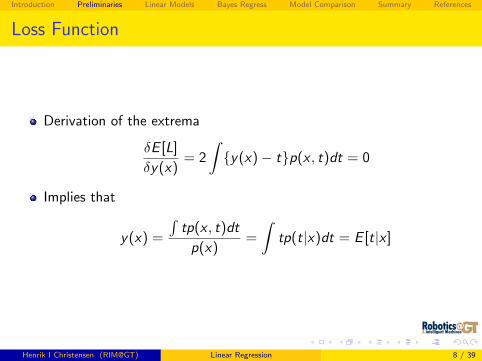
Loss Function

Derivation of the extrema

δE [L]

δy(x)= 2

∫{y(x)− t}p(x , t)dt = 0

Implies that

y(x) =

∫tp(x , t)dt

p(x)=

∫tp(t|x)dt = E [t|x ]



Loss Function - Interpretation

t

xx0

y(x0)

y(x)

p(t|x0)



Alternative

Consider a small rewrite

{y(x)− t}2 = {y(x)− E [t|x ] + E [t|x ]− t}2

The expected loss is then

E [L] =

∫{y(x)− E [t|x ]}2p(x)dx +

∫{E [t|x ]− t}2p(x)dx



Outline

1 Introduction

2 Preliminaries




6 Summary



Polynomial Basis Functions

Basic Definition:

φi (x) = x i

Global functionsSmall change in x affects all ofthem

−1 0 1−1

−0.5

0

0.5

1



Gaussian Basis Functions

Basic Definition:

φi (x) = e−(x−µi )

2

2s2

A way to Gaussian mixtures,local impactNot required to haveprobabilistic interpretation.µ control position and scontrol scale

−1 0 10

0.25

0.5

0.75

1



Sigmoid Basis Functions

Basic Definition:

φi (x) = σ

(x − µi

s

)where

σ(a) =1

1 + e−a

µ controls location and scontrols slope

−1 0 10

0.25

0.5

0.75

1



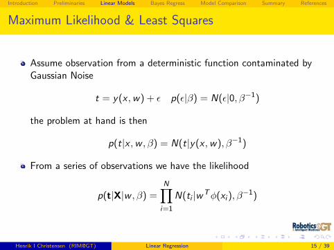
Maximum Likelihood & Least Squares (2)

This results in

ln p(t|w, β) =N

2lnβ − N

2ln(2π)− βED(w)

where

ED(w) =1

2

N∑i=1

{ti −wTφ(xi )}2

is the sum of squared errors



Maximum Likelihood & Least Squares (3)

Computing the extrema yields:

wML =(ΦTΦ

)−1ΦT t

where

Φ =

φ0(x1) φ1(x1) · · · φM−1(x1)φ0(x1) φ1(x2) · · · φM−1(x2)

......

. . ....

φ0(xN) φ1(xN) · · · φM−1(xN)



Line Estimation

Least square minimization:

Line equation: y = ax + bError in fit:

∑i (yi − axi − b)2

Solution: (y2

y

)=

(x2 xx 1

) (ab

)Minimizes vertical errors. Non-robust!



LSQ on Lasers

Line model: ri cos(φi − θ) = ρ

Error model: di = ri cos(φi − θ)− ρ

Optimize: argmin(ρ,θ)

∑i (ri cos(φi − θ)− ρ)2

Error model derived in Deriche et al. (1992)

Well suited for “clean-up” of Hough lines



Total Least Squares

Line equation: ax + by + c = 0

Error in fit:∑

i (axi + byi + c)2 where a2 + b2 = 1.

Solution: (x2 − x x xy − x y

xy − x y y2 − y y

) (ab

)= µ

(ab

)where µ is a scale factor.

c = −ax − by



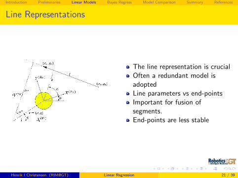
Line Representations

The line representation is crucialOften a redundant model isadoptedLine parameters vs end-pointsImportant for fusion ofsegments.End-points are less stable



Sequential Adaptation

In some cases one at a time estimation is more suitable

Also known as gradient descent

w(τ+1) = w(τ) − η∇En

= w(τ) − η(tn −w(τ)Tφ(xn))φ(xn)

Knows as least-mean square (LMS). An issue is how to choose η?



Regularized Least Squares

As seen in lecture 2 sometime control of parameters might be useful.

Consider the error function:

ED(w) + λEW (w)

which generates

1

2

N∑i=1

{ti − w tφ(xi )}2 +λ

2wTw

which is minimized by

w =(λI + ΦTΦ

)−1ΦT t



Outline

1 Introduction

2 Preliminaries




6 Summary



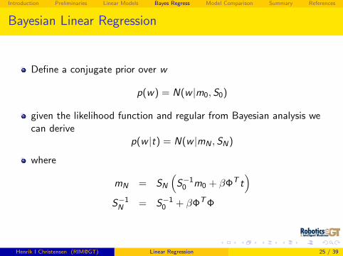
Bayesian Linear Regression

Define a conjugate prior over w

p(w) = N(w |m0,S0)

given the likelihood function and regular from Bayesian analysis wecan derive

p(w |t) = N(w |mN ,SN)

where

mN = SN

(S−1

0 m0 + βΦT t)

S−1N = S−1

0 + βΦTΦ



Bayesian Linear Regression (2)

A common choice is

p(w) = N(w |0, α−1I )

So that

mN = βSNΦT t

S−1N = αI + βΦTΦ



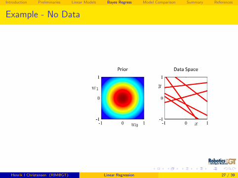
Example - No Data



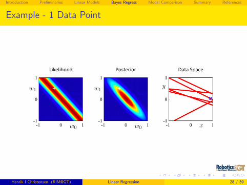
Example - 1 Data Point



Example - 2 Data Points



Example - 20 Data Points



Outline

1 Introduction

2 Preliminaries




6 Summary



Bayesian Model Comparison

How does one select an appropriate model?

Assume for a minute we want to compare a set of models Mi ,i ∈ 1, ...L for a dataset D

We could compute

p(Mi |D) ∝ p(D|Mi )p(Mi )

Bayes Factor: Ratio of evidence for two models

p(D|Mi )

p(D|Mj)



The mixture distribution approach

We could use all the models:

p(t|x ,D) =L∑

i=1

p(t|x ,Mi ,D)p(Mi |D)

Or simply go with the most probably/best model.



Model Evidence

We can compute model evidence

p(D|Mi ) =

∫p(D|w ,Mi )p(w |Mi )dw

Allow computation of model fit based on parameter range



Evaluation of Parameters

Evaluation of posterior over parameters

p(w |D,Mi ) =P(D|w ,Mi )p(w |Mi )

P(D|Mi )

There is a need to understand how good is a model?



Model Comparison

Consider evaluation of a model w. parameters w

p(D) =

∫p(D|w)p(w)dw ≈ p(D|wmap)

σposterior

σprior

Then

ln p(D) ≈ ln p(D|wmap) + ln

(σposterior

σprior

)



Model Comparison as Kullback-Leibler

From earlier we have comparison of distributions

KL =

∫p(D|M1) ln

p(D|M1)

p(D|M2)dD

Enables comparison of two different models



Outline

1 Introduction

2 Preliminaries




6 Summary



Summary

Brief intro to linear methods for estimation of models

Prediction of values and models

Needed for adaptive selection of models (black-box/grey-box)Evaluation of sensor models, ...

Consideration of batch and recursive estimation methods

Significant discussion of methods for evaluation of models andparameters.

This far purely a discussion of linear models



Deriche, R., Vaillant, R., & Faugeras, O. 1992. From Noisy Edges Pointsto 3D Reconstruction of a Scene : A Robust Approach and ItsUncertainty Analysis. Vol. 2. World Scientific. Series in MachinePerception and Artificial Intelligence. Pages 71–79.


linear models for regression - college of computinghic/8803-fall-09/slides/8803-09-lec03.pdf ·...

Documents