linear models for item scores: reliability, covariance
TRANSCRIPT

ACT Research Report Series 93-4
Linear Models for Item Scores: Reliability, Covariance Structure, and Psychometric Inference
David Woodruff
August 1993

For additional copies write: ACT Research Report Series P.O. Box 168 Iowa City, Iowa 52243
©1993 by The American College Testing Program. All rights reserved.

Linear Models1
Linear Models f o r Item Scores:
R e l i a b i l i t y , Covariance Structure, and
Psychometric Inference
David Woodruff American College Test ing
Running Head: LINEAR MODELS

♦

Linear Models2
Linear Models f o r Item Scores:
R e l i a b i l i t y , Covariance Structure,
and Psychometric Inference

Linear Models3
Abstract
Two ANOVA models for item scores are compared. The f i r s t i s an items by
subject random e f f e c t s ANOVA. The second is a mixed e f f e c t s ANOVA with items
f ixed and subjects random. Comparisons regarding r e l i a b i l i t y ,
Cronbach’ s a c o e f f i c i e n t , psychometric inference, and inter-item covariance
structure are made between the models. When considering the inter-item
covariance structures fo r the two ANOVA models, b r i e f comparisons with fac tor
analysis models are also made. I t is concluded that inference from a sample
o f items to a population of items requires homogeneous inter- item covariances,
that r e l i a b i l i t y has d i f fe r en t meanings under the two models, and that while
c o e f f i c i en t a is a lower bound for r e l i a b i l i t y under the second model, i t is
not under the f i r s t .
Key Words: Coe f f ic ien t Alpha, Covariance Structure, G en e ra l i z ab i l i t y ,
Linear Models, Psychometric Inference, R e l i a b i l i t y
Introduction
This paper compares two d i f fe r en t ANOVA models for items. The f i r s t
model is the two-way items by examinees random e f f e c t s (Model I I ) ANOVA. The
second model is the two-way items by examinees mixed e f f e c t s (Model I I I )
ANOVA. Very careful and complete s t a t i s t i c a l derivat ions of these models are
given by Schef fe ' (1956a, 1956b, and 1959). This paper draws heavily
from S c h e f f e '1s work. The two ANOVA models are compared to each other in
de ta i l and b r i e f l y to factor analysis models. Factor analysis models are
extens ive ly discussed by Harmon (1976) and Mulaik (1972). As considered here,
the fac tor analysis model is s t a t i s t i c a l l y more s imilar to the mixed ANOVA
model than to the random ANOVA model. Under the factor analysis model, items
are considered f ixed and non-random, while subjects are randomly sampled from
a population of subjects. See Mulaik and McDonald (1978), Williams (1978),
and McDonald and Mulaik (1979) for an a l te rnat ive formulation o f the factor
analysis model.
A l l of the models under consideration are l inear models. A model is
defined as l inear i f an examinee’ s expected score on an Item is a l inear
function o f item character is t ics . Item character is t ics may be f ixed
parameters as in the mixed ANOVA model or random variables as in the random
ANOVA model. The factor analysis model is here considered to be l inear in i t s
item parameters which are usually ca l led fac tor loadings even though these
l inear c o e f f i c i en ts are applied to fac tor scores, which are unobserved random
variables associated with examinees. An example of a nonlinear model is the
l o g i s t i c og ive item character iSt ic curve model (Lord and Novick, 1968). From
a theore t ica l viewpoint, l inear models usually do not accurately describe
dichotomously scored items, and most items are so scored. However, for
ca re fu l ly constructed tes ts , l inear models f o r item scores are often
Linear Models4

s u f f i c i e n t l y accurate to provide useful approximations. [See Feldt (1965),
Hsu and Feldt (1969), Hakstian and Whalen (1976), Seeger and Gabrielsson
(1968), Gabrielsson and Seeger (1976), McDonald and Ahlawat (197*0* McDonald
(1981, 1985), and Col l ins , C l i f f , McCormick, and Zatkin (1986). ]
The discussion o f the models presented here w i l l focus on three
character ist ics useful in psychometrics. The f i r s t is r e l i a b i l i t y . Under the
three models r e l i a b i l i t y i s defined as the squared corre la t ion between an
observed and a true score. A few relevant references regarding r e l i a b i l i t y
are Gutman (19*15), Novick and Lewis (1967) Bentler (1972), Jackson and
Agunwamba (1 977), and Bentler and Woodward (1980, 1983). Parametric
expressions for r e l i a b i l i t y and Cronbach's (1951) c o e f f i c i e n t alpha are given,
and the sampling d is tr ibut ion fo r the sample alpha c o e f f i c i e n t is discussed.
The second character is t ic i s the inter-item covariance matrix. For each
model, the assumed or resu lt ing covariance structure is discussed and compared
with factor analysis models. F ina l ly , psychometric inference is discussed.
Psychometric inference is considered as s t a t i s t i c a l inference to a population
of items from a sample o f items randomly drawn from the population. The more
general term g en era l i z ab i l i t y is not used since i t connotes s t a t i s t i c a l
inference fo r a wide array o f facets , not jus t items. There is a large body
o f l i t e ra tu re on psychometric inference. A few references are Hotel l ing
(1933), Tryon (1957), Lord and Novick (1968), Cronbach, Gleser, Nanda, and
Rajaratnam (1972), Mulaik (1972), Kaiser and Michael (1975), Rozeboom (1978),
McDonald (1978), and Brennan (1983). Both the approach and results presented
here, while most simi lar to , d i f f e r in part from those developed by Lord and
Novick (1968) and Cronbach et a l . (1972).
Br ie f descriptions of seven conclusions or ig ina l to this paper are:
1. Conditional variances for interaction e f f e c t s may be heterogeneous in the random ANOVA model.
Linear Models5

Linear Models6
2. The random ANOVA model requires the inter-i tem covariance matrix to have homogeneous o f f -d iagonal elements, while the mixed ANOVA model places no r es t r ic t ion s on the inter-i tem covariance matrix except pos i t i v e semi-definiteness. Hence, any fac tor analysis model may be subsumed under the mixed ANOVA model but not the random ANOVA model.
3. Interact ion e f f e c t s in the random ANOVA model are analogous to s p e c i f i c factors in a certa in s ing le common factor factor analysis model, while the examinee main e f f e c t is analogous to the s ingle common factor .
4. The squared corre la t ion between observed scores and true scores i s a useful d e f in i t ion of r e l i a b i l i t y under the random ANOVA model as well as under the mixed ANOVA model, but the de f in i t i on o f true score d i f f e r s under the two models.
5. R e l i a b i l i t y as defined in 4. has d i f f e r en t meanings under the two models. In the mixed ANOVA model, interact ion ( s p e c i f i c ) variance is included in true score variance, while in the random ANOVA model i t i s not.
6. The parametric value o f Cronbach's alpha c o e f f i c i e n t i s a lower boundto the parametric value of r e l i a b i l i t y (as defined in 4) under themixed ANOVA model but not under the random ANOVA model.
7. Given certa in normality assumptions, a transformation of the samplealpha c o e f f i c i e n t has an F d is tr ibut ion under the random ANOVA model.For the mixed ANOVA model, the F d is tr ibut ion only holds i f inaddition to certa in normality assumptions there are e i ther no interactions or the inter- item covariance matrix has special r es t r ic ted forms.
The pract ica l implications of these conclusions for the analysis of tes t data
w i l l be discussed in the l a s t sect ion of this paper.
The Items by Examinees Random ANOVA Model
The model presented here i s essen t ia l ly the same model developed by
Schef fe ' 0 959, chap. 7) . I t assumes that a random sample of n items chosen
from a countably i n f in i t e population o f items i s administered to a random
sample of N examinees chosen from a countably i n f in i t e population of
examinees. The sampling o f items and examinees i s assumed to be completely
independent. Let x^j represent subject j ’ s observed score on item i . A
preliminary form of the model is

Linear Models7
x i j = t u + e i j 1 - 1 ............ n J = 1 ............. N - ( 1 >
The quanti t ies t j j and e^j are, r espec t ive ly , the true score and the error
score of examinee j on item i. D i f ferent de f in i t ions fo r true and error
scores under the random ANOVA model w i l l be admitted la t e r . Within the
present context, true and error scores are not absolutes; their de f in i t ions
may vary depending on the inferences being made. The various true and error
scores considered in this paper are not necessari ly an exhaustive set of
possible true and error scores under the models presented.
I f examinee j responds independently and repeatedly to item i , these
rep l icat ions are indexed by the subscript k. For cognit ive tes ts such random
rep l ica t ions are ra re ly ava i lab le , though they occasional ly may be obtained
for a f f e c t i v e scales. The present development assumes that such rep l ica t ions
are not ava i lab le from the data. In the theoret ica l development of the model,
these rep l ica t ions are allowed to be present. In part icu lar , the model
assumes that fo r the sequences of independent random variables
e. , e . . _ ............e . . . , . . . : ECe,-H1.) = 0 for a l l i , j , and k , and thati j1 i j 2 i jk i j k
V a r ( e . . . ) = E(e* ) = o2( e . , ) , i . e . , that the error variances are i jk i j k i j
heterogeneous over the domains of i and j . For notational s imp l ic i ty , the
subscript k w i l l usually be suppressed, since fo r the remainder of the paper
i t w i l l usually take the value o f one.
The above imply that Ej ( e i J = 0 and that E^e^ J = 0, where notation1 1J J 1 J
such as and Var^ means that the expectation and variance are taken over the
population whose members are indexed by the subscript i . When no subscript is
present the expectation is over random rep l ica t ions . The above also imply
that the true and error scores are uncorrelated, i . e . , Cov. ft . .,e.i i j i j
= CoVj ( t i j , e . = 0 fo r a l l j ,j ' and i . i ' , r espect ive ly . I t i s further
assumed that a l l errors are independent within and across a l l populations.
Linear Models8
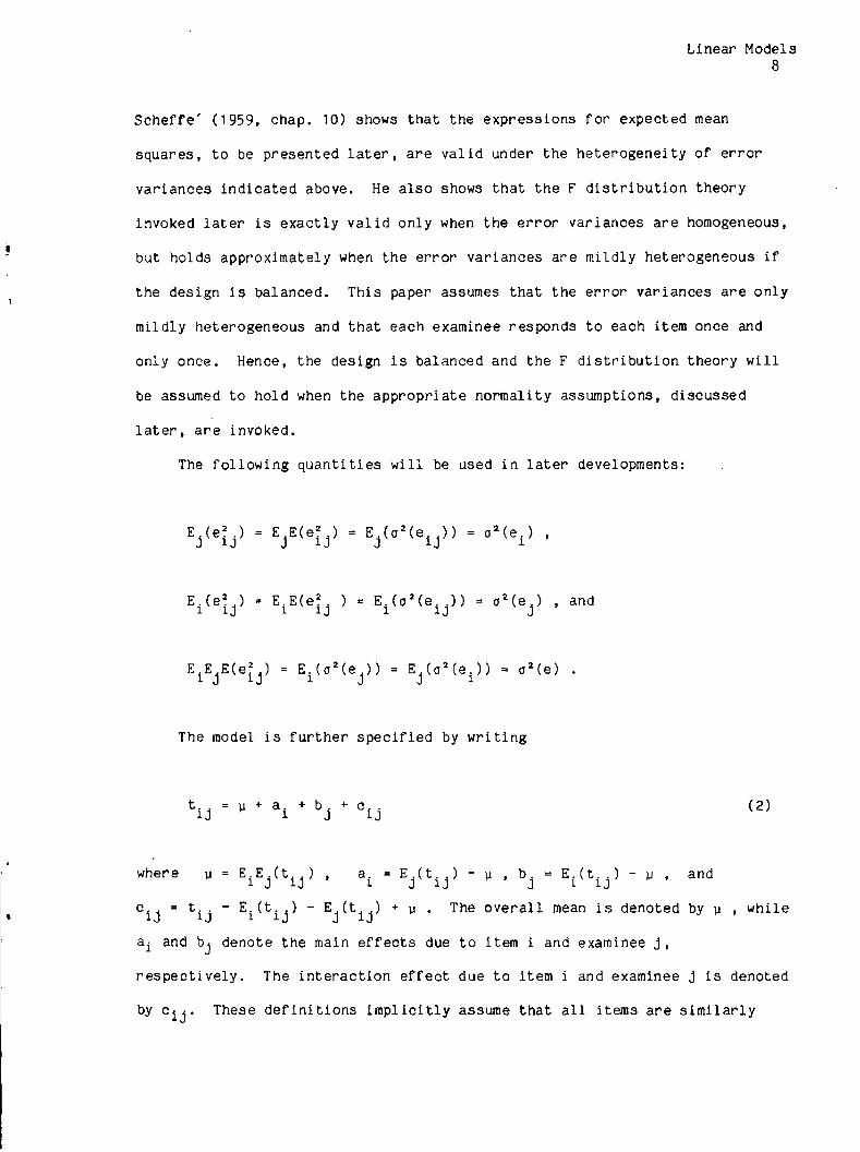
Sche f fe ' (1959, chap. 10) shows that the expressions for expected mean
squares, to be presented la t e r , are va l id under the heterogeneity o f error
variances indicated above. He also shows that the F d is tr ibut ion theory
invoked la te r i s exact ly va l id only when the error variances are homogeneous,
but holds approximately when the error variances are mildly heterogeneous i f
the design is balanced. This paper assumes that the error variances are only
mildly heterogeneous and that each examinee responds to each item once and
only once. Hence, the design i s balanced and the F d is tr ibut ion theory w i l l
be assumed to hold when the appropriate normality assumptions, discussed
la t e r , are invoked.
The fo l low ing quanti t ies w i l l be used in la te r developments:
E .E jE (e j j ) = E . ( o 2(e ) ) = E ^ a ^ e . ) ) « 02(e ) .
The model i s further spec i f ied by wr it ing
t. . = y + a. + b . + c, . (2)ij i J ij
where y = E E ( t ) , a = E ( t ) - y , b = E ( t ) - y , and J J 1J J -L I J
c ^ = t _ - Ei ( t i j ) - E jC t^ ) + y . The ove ra l l mean i s denoted by y , while
a and bj denote the main e f f e c ts due to item i and examinee j ,
r espec t ive ly . The interaction e f f e c t due to item i and examinee j i s denoted
by c^ j . These de f in i t ions im p l i c i t l y assume that a l l items are s im i lar ly
Linear Models9
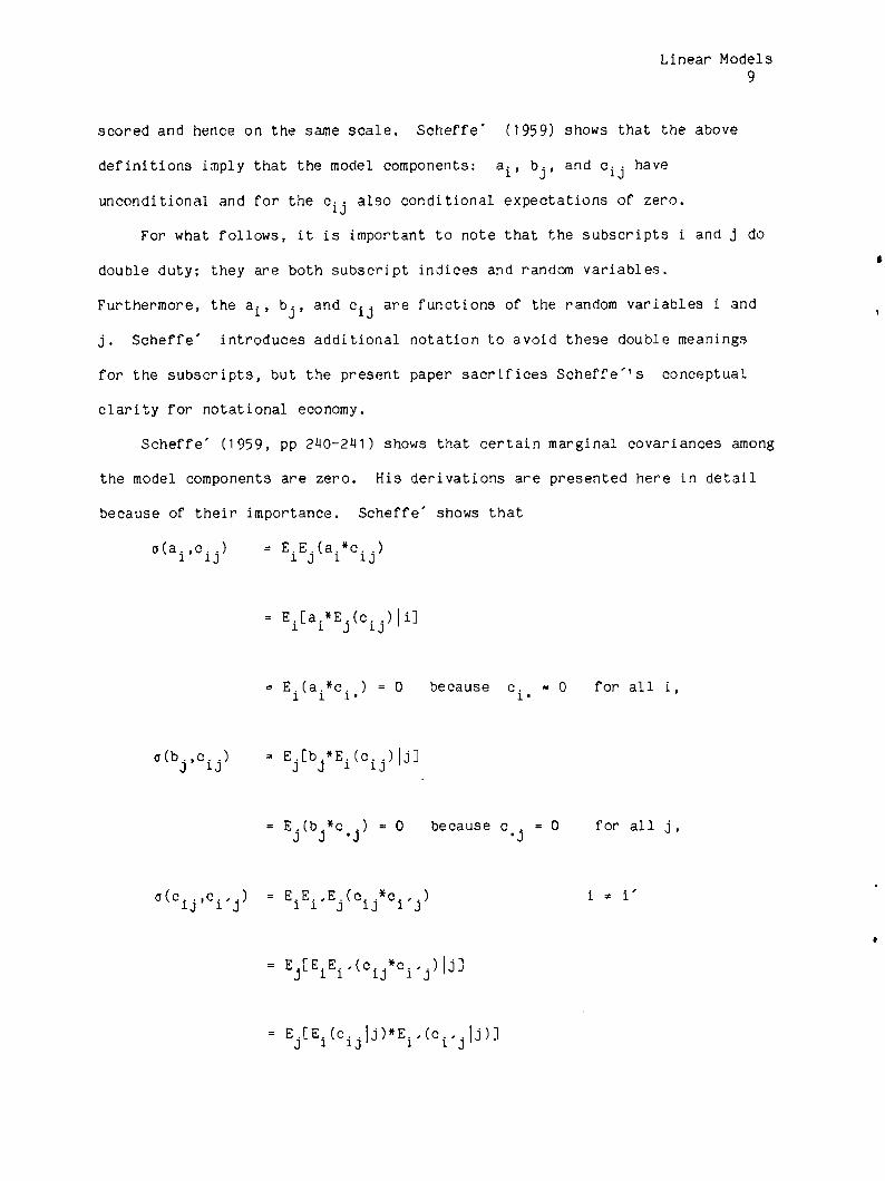
scored and hence on the same scale . Schef fe ' (1959) shows that the above
For what fo l lows, i t i s important to note that the subscripts i and j do
j . Schef fe ' introduces additional notation to avoid these double meanings
for the subscripts, but the present paper sac r i f i c e s S c h e f f e ' ’ s conceptual
c l a r i t y fo r notational economy.
Schef fe ' (1959, pp 240-241) shows that certa in marginal covariances among
the model components are zero. His derivations are presented here in deta i l
because of the ir importance. Schef fe ' shows that
de f in i t ions imply that the model components: a^, b j , and c^j have
unconditional and fo r the c-- also conditional expectations of zero.v
*double duty; they are both subscript indices and random variables.
Furthermore, the a^, b j , and c^j are functions of the random variables i and
- E, [a *E . (o , , )| i ], L « . LJ » \ . .
1 i J i j
- E . (a . *c . ) = 0 l i l ■ because c. = 0 for a l l i , i *
= E . (b .*c .) - 0 J J *J
because c . = 0 •J
for a l l j ,
i * i'

Linear Models10
E.Cc .*c .) = 0 because c . = 0 fo r a l l j ,j -J -J *J
Ei [ E . ( CiJ |1) « E . . ( c 1J, U ) ] j . y
= E. (c . *c, ) = 0 because c, = 0 fo r a l l i .i i • i • i •
In the above, the notation r e fe rs to the expectation over the b ivar ia te
d is t r ibut ion obtained from sampling pairs of items from the population o f
items where the members of each pair are d is t inc t .
Sche f fe ' (1959) does not discuss the fo l low ing model component
condit ional covariances:
°<a i 'Ojj lJ) ■ E ^ a ^ o ^ l J ) ,
o(b . ,c. . I i ) = E . (b , * c . . I i ) ,J i J 1 J J iJ
a ( c . . , c . . . | l , i ' ) - E . ( o . . * o . . . | i , i ' ) , and
These conditional covariances are of considerable concern because as w i l l be
seen l a t e r the ir values determine the inter-i tem covariance matrix.
Though a formal proof w i l l not be given, i t i s asserted here that the
above conditional covariances are also zero under S c h e f f e ' f s (1959) model.
Four considerations lead to th is conclusion. F i rs t i t does not appear
possible to generate model component data such that Sche f fe ' *s marginal
covariances are zero but the above conditional covariances are not.
and
0<C c )
Linear Models11
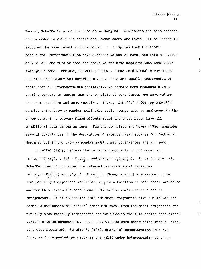
Second, S ch e f f e ' ' s proof that the above marginal covariances are zero depends
on the order in which the conditional covariances are taken. I f the order i s
switched the same resu l t must be found. This implies that the above
conditional covariances must have expected values of zero, and th is can occur
only i f a l l are zero or some are pos i t ive and some negative such that their
average i s zero. Because, as w i l l be shown, these conditional covariances
determine the inter-item covariances, and tes ts are usually constructed of
items that a l l in tercorre la te p os i t i v e ly , i t appears more reasonable in a
tes t ing context to assume that the conditional covariances are zero rather
than some pos i t ive and some negat ive. Third, Schef fe ' (1959, pp 242-2^3)
considers the two-way random model interaction components as analogous to the
error terms in a two-way f ixed e f f e c t s model and these la t e r have a l l
conditional covariances as zero. Fourth, Cornf ie ld and Tukey (1956) consider
several covariances in the der ivation of expected mean squares f o r fa c to r ia l
designs, but in the two-way random model these covariances are a l l zero.
Schef fe ' (1959) defines the variance components of the model as:
o2(a) = E ( a p , o2(b) = E . (b2) , and o2(c ) = E .E . ( c ? . ) , In defin ing a2( c ) ,J J J J
Schef fe ' does not consider the interact ion conditional variances
o2( c . ) = E ( c ? . ) and o2( c ) = E . ( c ? . ) . Though i and j are assumed to be i J J j J
s t a t i s t i c a l l y independent var iables, c^j is a function of both these variables
and fo r th is reason the conditional interaction variances need not be
homogeneous. I f i t i s assumed that the model components have a multivar ia te
normal d is tr ibut ion as Schef fe ' sometimes does, then the model components are
mutually s t a t i s t i c a l l y independent and th is forces the interact ion conditional
variances to be homogeneous. Here they w i l l be considered heterogenous unless
otherwise spec i f ied . S c h e f f e ' ’ s (1959, chap. 10) demonstration that his
formulas for expected mean squares are va lid under heterogeneity o f error

Linear Models1 2
variances implies the same under heterogeneity of in teract ion conditional
var iances.
Of particular in te res t in the random model ANOVA are the mean squares for
examinees and the mean squares fo r items by examinees which are denoted MS
and MSC, respec t iv e ly . Schef fe ' (1959) derives the fo l low ing expressions for
the expected value o f these mean squares: E ^M S ^ ) = no2(b) + a2(c ) + a2(e )
and E^(MS ) = o2(c ) + o2( e ) , where E ^ denotes that these expectations are
the means o f an i n f in i t e number of b ivar ia te random samples consisting o f n
items and N subjects.
These mean squares are o f in terest because Hoyt (19*11) has shown that theA
sample value o f Cronbach's (1951) c o e f f i c i en t a, denoted a herein, is given by
a = [(MS, - MS ) /MS.] = 1 - (MS /MS, ) . The parametric counterpart of b c b c b
a depends upon the s t a t i s t i c a l model used to describe the data. For the
random ANOVA model th is parameter i s denoted a ( the subscript RA denoting
that th is d e f in i t i on i s sp ec i f i c to the random model ANOVA. The
parameter aRA is defined by
terms of E^CMS^ and EnN M c^ whose de f in i t ions in turn depend upon the RA
subscript. Feldt (1965) has shown that under the additional assumptions of
independent normal d is tr ibut ions fo r the {a^}, { b j } , { c ^ j } , and { e ^ j } ,
(1 ~ * s d istr ibuted as F[N-1, (n -1 ) (N -1 ) ] . Under these
assumptions, the conditional variances for both the interactions and errors
aRAa2(b) + a2(c)/n + a2(e)/n
a2 (b)(3)
The ra t iona le f o r this d e f in i t i on is that a converges in probab i l i ty to aD.RA
under the RA model. This i s discussed further below. Since aDA is defined inRA
model, the de f in i t i on of aRA is t ied to the RA model and hence the RA

Linear' Models1 3
are considered homogeneous, but s l i gh t heterogeneity should produce at most
only mild departures from the F d is t r ibu t ion . Using the expression fo r the
mean of an F d is tr ibut ion i t fo l lows that E M(ot) = [ (N - 1)/N - 3 ) ] a 0» “nN nfl
[2/(N - 3 ) ] . This shows that a is an asymptotically (as N *► 00) unbiased
estimator of m . Even without the normality assumptions, a is s t i l l a HA
consistent estimator for aDA since i t is a method of moments estimatorHA
for (S e r f l in g , 1933), and equivalent ly converges in probabi l i ty to ot^ •
The random ANOVA (RA) model has been presented in some de ta i l . Tt is now
of in teres t to compare that model to the factor analysis (FA) model. This
comparison may be made by examining the conditional covariance matrix for the
n sampled items, the conditioning being on the n items selected from the
in f in i t e population o f items. Let the observed scores on the n items be
represented by the column vector x . The conditional covariance matrix is
Z i = E . [ ( x . - E . ( x . ) ) ' ( x . - E . ( x . ) ) J . The diagonal elements of th is matrix ~x j n j —j j ' j j —J
are Var ( x ^ ) = o2(b) + o2(c^) + o2( e . ) . Because i t i s assumed here that
under the RA model covj (c • j , c ^ ) = 0 for any pair of items randomly
selected from the population o f items, i t fo l lows triat th is covariance w i l l
be zero for a l l pairs of items in the randomly selected sample of n items,
and consequently that the o f f -d iagonal elements of th is matrix are
Cov.(x. . , x . , . ) = o2(b) . The rather simple form of th is conditional J iJ i J
covariance matrix may be represented as £x jn = o2(b)J + A [a2(c^) + a2( e ^ ) ]
where J represents a matrix o f a l l ones and A is a diagonal matrix with the
indicated elements. I t fo l lows that the conditional covariance matrix for the
true scores on the n items is
? t |n = o2(b)J + A (o2( c i ) )

Linear Models1 4
Hocking (1985) presents covariance structures fo r a wide var ie ty o f random and
mixed ANOVA models. He assumes homogeneity among the error and conditional
interact ion variances. Given his assumptions, his results agree with those
presented here.
The RA conditional covariance structure i s ident ica l to the covariance
structure of a one common fac tor FA model with homogeneous fac tor loadings and
n sp e c i f i c factors d is t inc t from the errors . This i s Spearman's (190M) model
but with the additional r e s t r i c t i o n that the items a l l corre la te equally with
the general fac tor . More s p e c i f i c a l l y , the subject main e f f e c t variance in
the RA model is analogous to the common factor variance in the FA model while
the conditional interact ion variances in the RA model are analogous to
sp ec i f i c variances in the FA model. Another way to character ize this
conditional covariance structure i s as an essen t ia l ly tau equivalent model
(Lord and Novick, 1968) but with the addition o f n sp e c i f i c factors with
possibly heterogeneous variances.
I f the sp e c i f i c fac tors have homogeneous variances, then the conditional
covariance structure fo r the true scores is equivalent to the equicorrela t ion
model (Morrison, 1976). Under the equicorre la t ion model, the f i r s t and
la rges t eigenvalue of L i , denoted ji,, is equal to no2(b) + a2(c ) . The""" T/1 n
second d is t inc t eigenvalue o f ? t |n has m u l t ip l i c i t y n-1 and i s given
by o2(c ) . I t i s denoted X2 .
The simple form of the conditional covariance matrix in the RA model
resu l ts from the uncorrelatedness of the model components. Though th is
covariance structure i s a rather r es t r i c t ed specia l case o f the many more
ve rsa t i l e covariance structures permitted by FA models, the RA model permits
e x p l i c i t s t a t i s t i c a l inference to a population o f items. The price fo r th is
gain in " g en e ra l i z a b i l i t y ” is the assumption of a simple covariance structure

Linear Models15
among the items.
The in fe ren t ia l d i f ferences between considering items random and
considering items f ixed may be i l lus tra ted by how r e l i a b i l i t y may be defined
under these conditions. For subject j , l e t the item domain true score be
defined as t , = E . ( x . , ) = u + b. . This implies that the item domain error J i i j J
score fo r subject j i s e . * x . - T . = a + c , + e . . Note that fo r random J J J j j J
rep l icat ions E (e . ) = a . + c . . , and that fo r examinees E . ( e . ) = a. .j ■ s3 J J
Furthermore, considering just a one-item test , Cov (e. .,e. . , ) »i J J
o2(a ) fo r a l l j * j' . These conditions v io la t e the usual assumptions of
c lass ica l tes t theory (Lord and Novick, 1968, chap. 3 ) , because here the
errors do not have means of zero and the errors are in te r -co r re la ted .
However, C ov j ^T j *e j = 0 and-this crucia l result implies that i f interest
focuses on the r e l i a b i l i t y o f a sp ec i f i c t e s t composed o f n randomly se lected
items with respect to the item domain true scores, then a useful d e f in i t i on of
r e l i a b i l i t y i s R e l ( x t . , t .) = [Cor (x^ . , t . ) ] 2 . R e l i a b i l i t y so definedj J J * 3 J
measures the accuracy with which re la tionships between observed t e s t scores
are ind ica t ive of re la tionships between item domain true scores.
Since CoVj (xtj , T j ) = o2(b ) ,
V a r j ( x #j ) ® o2(b) + (1/n2)£?o2(c,.) + (1/n2)J?o2(e^ )
and V a r . ( T . ) = o 2(b) , i t fo l lows that J «J
R e K x ^ T j ) ------------------------------
a2(b) + (1/n2) ^ a 2( c i ) + (1/n2)£V ( e . )
= Var^ . ( i j )/VaT j (x . j ) ,
(5)

Linear Models16
which i s the usual r a t i o of true score variance to observed score variance. I f
the error variances and the conditional interaction variances are homogeneous
then = Re l (x . . t .) , otherwise an, i s only an approximation to th is RA •J J RA
r e l i a b i l i t y , a lb e i t not a bad one.
An a l te rnat ive de f in i t i on o f r e l i a b i l i t y under the RA model which i s more
appropriate when concern is not with the r e l i a b i l i t y of a particular randomly
constructed te s t but rather with the population o f such tests i s
E^[Rel( * . j »Tj ) ] * Here, En denotes that the expectation is over the
population o f randomly constructed tests consisting o f n items. This
d e f in i t i on o f r e l i a b i l i t y is appropriate when the same tes t w i l l be
administered to every examinee, but concern i s with the r e l i a b i l i t y o f any
randomly constructed te s t rather than a part icu lar tes t that i s randomly
se lected. The s ituat ion in which d i f f e r e n t examinees take d i f f e r en t randomly
constructed te s t forms is not often encountered in pract ice and is not
addressed in th is paper (but see Lord and Novick, 1968, p. 208). I f the error
variances and the conditional interact ion variances are homogeneous, then
E [Re l (x . ,t . ) ] = aDA . This fo l lows since Rel(x , , x . ) = aQ. fo r each and n • J j HA • j J H A
every randomly constructed t e s t consisting o f n items. I f homogeneity does
not hold, an exact expression fo r E (R e l ( x # . , t . ) ) requires additional modeln J J
spec i f i ca t ions which w i l l not be attempted in th is paper. However, i t may be
shown by using the de l ta method of Kendall and Stuart (1977, Vol. I ) that aD.RA
is a f i r s t order approximation for En[ R e l ( x ^ , i j ) ] under heterogeneity.
I f the data are accurately described by the RA model, but the usual
d e f in i t i on o f r e l i a b i l i t y (Lord and Novick, 1968, chap. 3) is adopted, then

Linear Models17
Rel(x . , t ) = [Cor (x , , t ) ] 2 = Var ( t , )/Var (x . ) (6)J " J J J \j x j J
o 2(b) + ( t / n 2 ) [ % 2 (c )1 i
a2( b) + (1 /n2) ] ^ 2 (c.) + (1 / n 2 Jl'ja2 (e . )
Usually, R e K x ^ . t ^ j ) > aRft . However, i f there is no item by examinee
interact ion and the error variances are homogeneous then Rel(x . ,t .) = aD. .*0 *j ha
A comparison o f (6) to (5) shows that the interact ion ( s p e c i f i c )
variances are included in the numerator of Rel(x . , t .) but excluded from the* J * J
numerator of R e l ( x #j , T j ) . This d i f ference is due to the d i f ference in
de f in i t ions between t . and i . . I f the true score i s sp ec i f i c to the tes t ,•J J
i . e . , t , , then the interact ion ( s p e c i f i c ) variances are included in the true
score variance. When the true score i s defined over the population o f items,
i . e . , , then the interaction ( s p e c i f i c ) variances do not contribute to t*ne
true score variance.
Two b r ie f observations regarding the RA model are o f in terest . I f no
interactions are present the RA model may be viewed as a l inear analog of the
one parameter Rasch model (Lord and Novick, 1968, p H02) with e x p l i c i t item
and examinee sampling. Second, the symmetry o f the RA model al lows
consideration o f not only the inter-i tem covariance matrix but also the
s im i lar ly constrained inter-examinee covariance matrix.
This section o f the paper has presented a deta iled development o f the RA
model and a b r ie f comparison of the RA model to the FA model. The development
demonstrates that under the RA model general izat ion in a s t a t i s t i c a l manner
over a population of items requires a simple and spec ia l ized covariance
structure among the items. In the next sect ion, the mixed ANOVA (MA) model is
considered.
Linear Models18
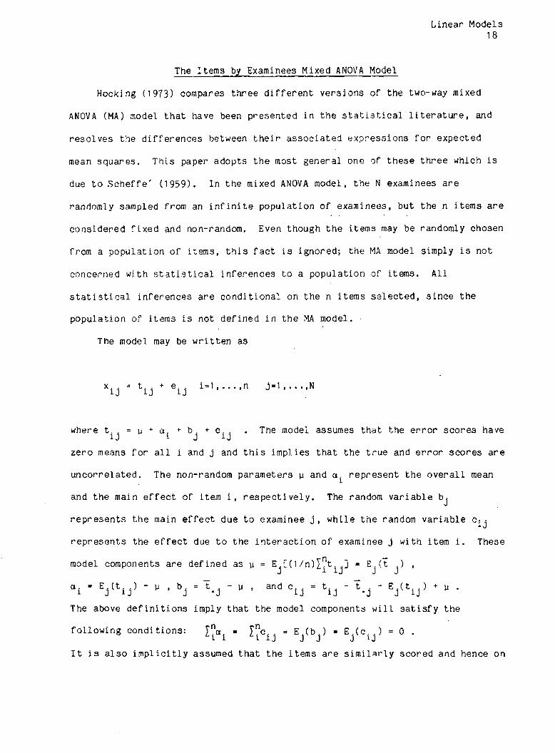
The Items by Examinees Mixed ANOVA Model
Hocking (1973) compares three d i f f e r en t versions of the two-way mixed
ANOVA (MA) model that have been presented in the s t a t i s t i c a l l i t e ra tu r e , and
resolves the d i f fe rences between the ir associated expressions fo r expected
mean squares. This paper adopts the most general one of these three which is
due to Sche f fe ' (1959). In the mixed ANOVA model, the N examinees are
randomly sampled from an in f i n i t e population o f examinees, but the n items are
considered f ixed and non-random. Even though the items may be randomly chosen
from a population o f items, th is fa c t i s ignored; the MA model simply i s not
concerned with s t a t i s t i c a l inferences to a population of items. A l l
s t a t i s t i c a l inferences are conditional on the n items se lected, since the
population of items is not defined in the MA model. ■
The model may be written as
x . . » t . . + e . . i = l , . . ., n j = l , . . . , Ni j i j i j
where t . . = y + a . + b . + c . . . The model assumes that the error scores havei j i j i j
zero means fo r a l l i and j and th is implies that the true and error scores are
uncorrelated. The non-random parameters y and ou represent the ove ra l l mean
and the main e f f e c t of item i , r espec t ive ly . The random var iable bj
represents the main e f f e c t due to examinee j, while the random variable c^j
represents the e f f e c t due to the in teract ion o f examinee j with item i . These
model components are defined as u = E . [ ( 1 /n)Tnt . .] = E . ( t .) ,J i i j J J
a. = E . ( t . .) - y , b. = t . - y . a n d c . . = t . . - t . - E . ( t . . ) + u . i J ij J ‘j ij ij *J J ij
The above de f in i t ions imply that the model components w i l l sa t i s fy the
fo l low ing conditions: Tna = ync = E (b ) = E (c ) = 0 .i i '■l ij j j J ij
I t i s also im p l i c i t l y assumed that the items are s im i la r ly scored and hence on

Linear Models19
the same scale. Allowing for heterogeneous error variances y ie lds the
fo l lowing: o2( e . ) = E . ( e ? . ) and a2(e ) = (1/n)£na2( e .) .- l J 1J * - 1 1
I f the error variances are homogeneous, then a2( e i > = a2(e ) for a l l i .
Let t j represent the n dimensional column vector of examinee j ’ s true
scores on the n items. The true score covariance matrix is
I = { o . , , } * E . [ ( t . - E . ( t . ) ) ' ( t . - E . ( t . ) ) ] . The only r e s t r i c t i o n placed J O J J J J O
on £ is that i t be pos i t ive semi-def in ite . The covariance among the items may
be o f a very general form, including any multiple common factor model. This
is quite d i f f e r en t from the RA model where a simple sp ec i f i c conditional
covariance structure is assumed. Removing the randomness of the items permits
a much more general covariance structure among the items, but el iminates any
s t a t i s t i c a l inferences concerning the population o f items.
From the de f in i t ions of the random model components, the variances and
covariances for these components may be expressed as functions of the
{ o u , } . Schef fe ' (1959) shows that
C o V j ( c _ , c i , j ) = E j ( c ^ * c ^ , j ) = - a i + a , and (8)
Cov (b ,c ) = E , (b . *c . ) = a. - a . (9)J J 1J J J 1J 1*
Schef fe ' (1959) defines the variance components as
o2 (b) =VarJ ( V
and ( 10 )
o2 ( c ) = [ 1 / ( n - 1 ) ] E j v a r (c ) = [ 1 / ( n - 1 ) ] ^ ( a. . - o ##) (1 1 )
Linear Models20
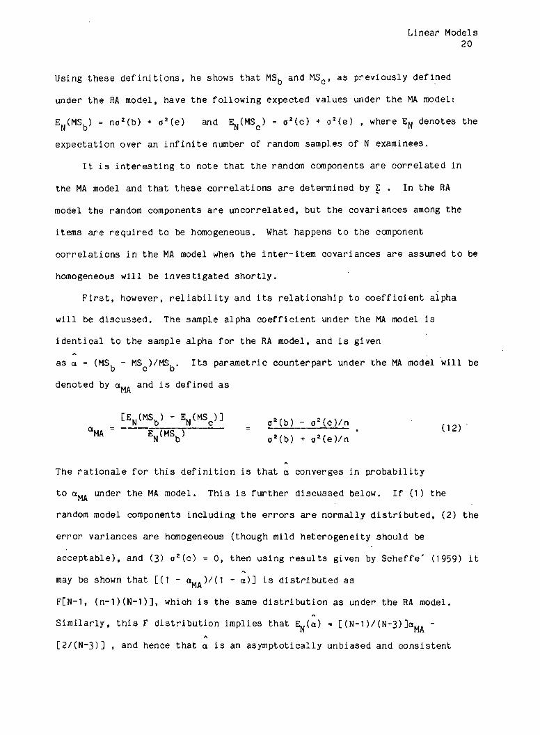
Using these de f in i t ions , he shows that MSb and MSC, as previously defined
under the RA model, have the fo l low ing expected values under the MA model:
E.,(MS. ) = no2(b) + oz (e ) and Em(MS ) = a2( c ) + o2( e ) , where Ew denotes the N b N c w
expectation over an in f i n i t e number of random samples of N examinees.
I t i s in terest ing to note that the random components are corre la ted in
the MA model and that these corre lat ions are determined by E . In the RA
model the random components are uncorrelated, but the covariances among the
items are required to be homogeneous. What happens to the component
corre lat ions in the MA model when the in ter- item covariances are assumed to be
homogeneous w i l l be investigated short ly .
F i r s t , however, r e l i a b i l i t y and i t s re lationship to c o e f f i c i e n t alpha
w i l l be discussed. The sample alpha c o e f f i c i en t under the MA model is
ident ica l to the sample alpha fo r the RA model, and i s given
as a = (MS^ - MSc )/MSb. I t s parametric counterpart under the MA model w i l l be
denoted by a... and i s defined as MA
[Eki(MSJ - Em(MS ) ] 2,k v 2, wN b N c o ( b ) ~ q (c )/n (\o\aMA E„(MSJ Zf. . A 2 / w 'N b a2(b) + a2(e)/n
The ra t iona le f o r this d e f in i t i on is that a converges in probabi l i ty
to oi^ under the MA model. This i s further discussed below. I f (1) the
random model components including the errors are normally d is tr ibuted , (2) the
error variances are homogeneous (though mild heterogeneity should be
acceptable), and (3) o2(c ) = 0, then using results given by Schef fe ' (1959) i t
may be shown that [ (1 - ~ i s d istr ibuted as
F[N-1, (n -1 ) (N -1 ) ] , which i s the same d is tr ibut ion as under the RA model.
S im i lar ly , th is F d is tr ibut ion implies that E ^ a ) ■ [ (N-1) / (N~3) l a ^ -A
[ 2 / (N—3 ) ] , and hence that a i s an asymptotically unbiased and consistent

estimate o f a... . K r is to f (1963) has previously derived these resu lts . I f MA
o2(c ) * 0, then the F d is tr ibut ion s t i l l holds i f I has the highly symmetric
structure discussed by Schef fe ' (1959, p 26*0 or i f £ has the type H form
described by Huynh and Feldt (1970); but as w i l l be seen la te r i s then a
s t r i c t lower bound to r e l i a b i l i t y . However, even i f the foregoing assumptions
are not f u l f i l l e d , a is s t i l l a consistent estimator of a.„ since i t is aMA
method o f moments estimate for (S e r f l in g , 1983). and equiva lent ly
converges in probab i l i ty to . F ina l ly , i t should be noted that
i f o2(c ) = 0, then a l l the c^j = 0 and the MA model is ident ica l to the
essen t ia l ly tau equivalent model discussed by Lord and Novick (1968).
Under the MA model, the mean true score of examinee j is
t . = (1/n)T?E(x. where, as discussed under the RA model, E denotes •j i l j k
expectation over the errors associated with random rep l ica t ions .
Let Xj denote the n dimensional column vector of the j - t h examinee’ s observed
scores on the n items. Let Z denote the covariance matrix for the observed“ X
scores. I t fo l lows that = I + A (o2(e^ ) ) where A (o2(e . . ) ) i s a diagonal
matrix with the error variances as i t s elements. Following Lord and Novick
(1968, chap. 3), r e l i a b i l i t y under the MA model is defined as
Rel(x ,t ) - [ C o r j ( x . j , t ) ] * ’ = o2(b )/ [ o 2(b ) + o2(e )/n] (13)
= Var ( t . )/Var. (x , )J *J J 0
The above fo l lows from the expressions for the variance components given in
(10) and (11). Comparison of the las t expression in the f i r s t l i n e of (13)
with the expression for a*.,, given in (12) demonstratesMA
that = R e K x ^ j t ^ ) i f and only i f o2( c ) = 0 , i . e . , the items are
Linear Models21
Linear Models22
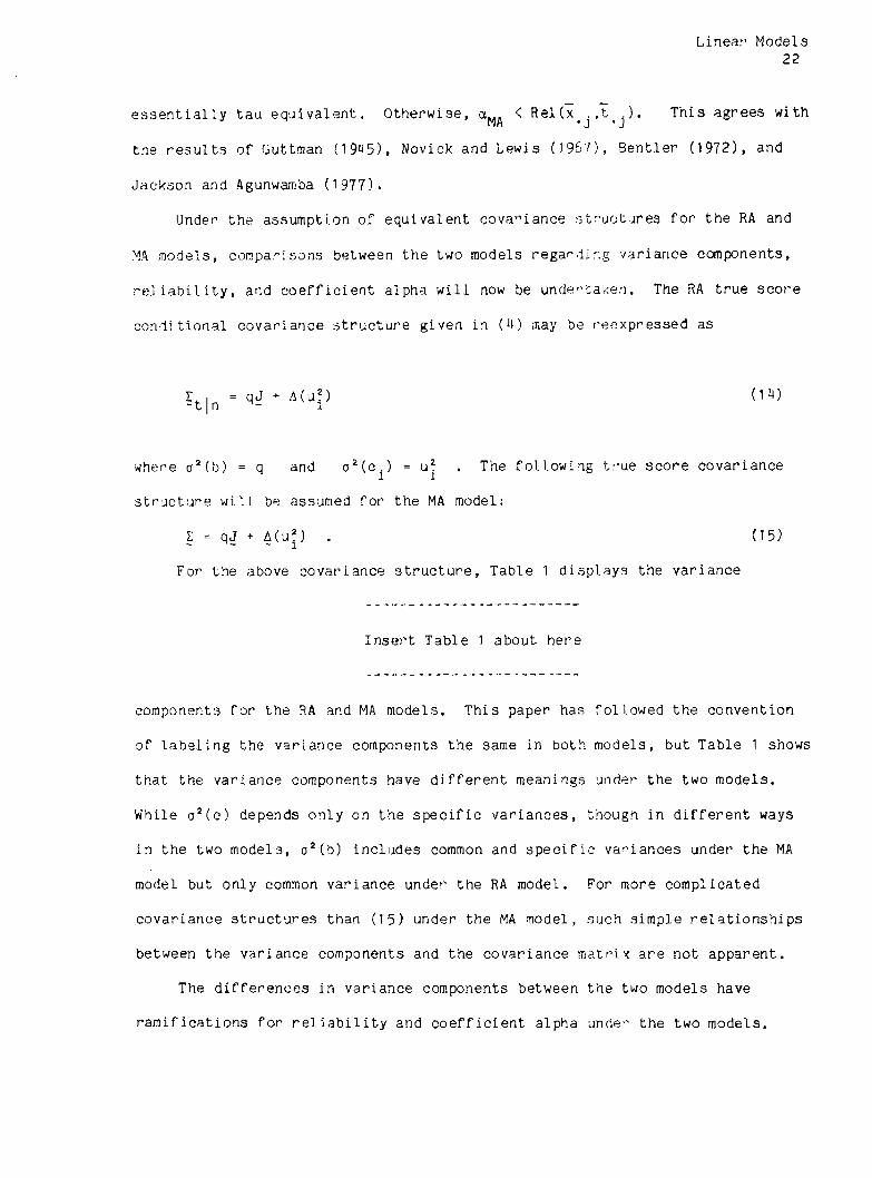
essen t ia l ly tau equivalent . Otherwise, aM. < Rel(x . ,t ) . This agrees withMA *j
the results of Guttman (19^5), Novick and Lewis (19b7) , Bentler (1972), and
Jackson and Agunwamba (1977).
Under the assumption of equivalent covariance structures fo r the RA and
MA models, comparisons between the two models regarding variance components,
r e l i a b i l i t y , and c o e f f i c i en t alpha w i l l now be undertaken. The RA true score
conditional covariance structure given in (4 ) may be reexpressed as
I | = qJ + A(u2) (1 *0-t|n - i
where o2(b) = q and o2(c..) « u2 . The fo l low ing true score covariance
structure witL be assumed for the MA model:
Z = qJ + A(u*) . (15)
For the above covariance structure, Table 1 displays the variance
Insert Table 1 about here
components fo r the RA and MA models. This paper has fol lowed the convention
of labe l ing the variance components the same in both models, but Table 1 shows
that the variance components have d i f f e r en t meanings under the two models.
While a2(c ) depends only on the spec i f i c variances, though in d i f fe r en t ways
in the two models, o2(b) includes common and s p e c i f i c variances under the MA
model but only common variance under the RA model. For more complicated
covariance structures than (15) under the MA model, such simple re lationships
between the variance components and the covariance mat r i x are not apparent.
The d i f fe rences in variance components between the two models have
ramif icat ions fo r r e l i a b i l i t y and c o e f f i c i en t alpha under the two models.

Linear Models23
Table 2 displays alpha and r e l i a b i l i t i e s fo r the two models under the
Insert Table 2 about here
indicated covariance structure. C oe f f i c ien t alpha d i f f e r s s t a t i s t i c a l l y under
the two models in that expectations are used in the denominator of aRA while
summations are used in the denominator of aw. Nonetheless, c o e f f i c i e n t alphaMA.
has a simi lar psychometric meaning under the two models since under both
models the numerator and denominator depend, with s l igh t var iat ions, on the
same elements o f the covariance matrix. Rel(x . , t . ) i s ident ica l under the* J *J
two models, but d i f f e r s from R e l (x^ . ,T . ) under the RA model as has alreadyJ J
been noted.
Under the RA model, the random model components are uncorrelated as was
previously discussed. For the MA model under the covariance structure in
(15),
C °V j (b j fc i j ) » [q + (u2/n)] - [q + (1/n2)£^u2]
= [u2 - (1/n)£nu?]/n andi **1 l
C oV j (c .^ ,c i ^ ) = q - (q + u2/n) - (q + u?,/n) + [q + (1/n2)£"u2]
= [ ( 1 / n )£ j j 2 - u2 - u2,]/n .
I f a l l the u2 are equal, then Cov, (b, , c { , ) = 0 and Cov (c ,c , ) = -u2/n i J J ij J i J i j
where u2 i s the common value fo r a l l the u2. The covariance -u2/n is due
the fac t that under the MA model Y^c . . = 0 for a l l i . As was notedL1 J
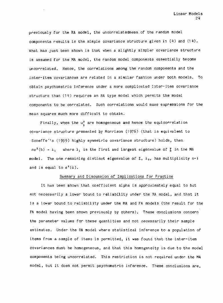
Linear Models24
previously for the RA model, the uncorrelatedness.of the random model
components resu l ts in the simple covariance structure given in (4 ) and (14).
What has jus t been shown is that when a s l i g h t l y simpler covariance structure
is assumed fo r the MA model, the random model components essent ia l ly become
uncorrelated. Hence, the corre la t ions among the random components and the
inter- item covariances are re la ted in a s imilar fashion under both models. To
obtain psychometric inference under a more complicated inter-i tem covariance
structure than (14) requires an RA type model which permits the model
components to be corre la ted. Such corre la t ions would make expressions fo r the
mean squares much more d i f f i c u l t to obtain.
F ina l ly , when the u? are homogeneous and hence the equicorre la t ion
covariance structure presented by Morrison (1976) (that i s equivalent to
Sche f fe ' * s (1959) highly symmetric covariance structure) holds, then
no2(b) = Aj where \ 1 is the f i r s t and la rges t eigenvalue o f I in the MA
model. The one remaining d is t in c t eigenvalue o f Z, X2» has m u l t ip l i c i t y n-1
and i s equal to o2( c ) .
Summary and Discussion o f Implications for Pract ice
I t has been shown that c o e f f i c i en t alpha i s approximately equal to but
not necessari ly a lower bound to r e l i a b i l i t y under the RA model, and that i t
i s a lower bound to r e l i a b i l i t y under the MA and FA models (the resu l t fo r the
FA model having been shown previously by others ) . These conclusions concern
the parameter values for these quanti t ies and not necessari ly the ir sample
estimates. Under the RA model where s t a t i s t i c a l inference to a population of
items from a sample o f items i s permitted, i t was found that the inter-i tem
covariances must be homogeneous, and that th is homogeneity i s due to the model
components being uncorrelated. This r e s t r i c t i o n i s not required under the MA
model, but i t does not permit psychometric inference. These conclusions are,

Linear Models25
o f course, sp ec i f i c to the models under-consideration, and other models may
y ie ld d i f fe r en t resu lts .
I t i s usually the case in education and psychology that inference from a
sample of items to a population of items is a desired goal in the analysis of
test data. However, th is may not always be true. A s i tuat ion in educational
measurement where psychometric inference may not be required is when a te s t is
d i v i s ib l e into well defined content heterogeneous subtests, and the subtest
scores are the measurements being analyzed. In th is s i tuat ion, an appropriate
model for the data could be a subtest by examinee two-way MA model. In
psychology, i f an a f f e c t i v e scale such as a personal ity inventory consists of
well defined psychologically d is t inc t subscales, then a subscales by subjects
two-way MA model could also be an appropriate model f o r the data.
I f psychometric inference i s desired and i f the RA model presented within
is going to be used to analyze the data, then i t is appropriate to invest igate
whether or not the data s a t i s f y the covariance structure assumed under the RA
model. This covariance structure is a l inear covariance structure, and Browne
(1972) has derived a procedure based on the pr inc ip le o f generalized leas t
squares (GLS) estimation that may be used to s t a t i s t i c a l l y test the f i t of the
data to the RA model covariance structure. Browne's (1972) method i s non
i t e r a t i v e and hence r e l a t i v e l y simple computationally. Joreskog (1978)
discusses s t a t i s t i c a l tests fo r covariance structures based on GLS and maximum
l ike l ihood (ML) estimation methods. The computer program LISREL VI
(Joreskog and Sorbom, 1986) implements those methods as well as others, and
is access ib le through the SPSSX (SPSSX Inc, 1986) computer program. Bentler
(1983) and Browne (1984) have developed GLS test procedures with weaker
d is tr ibut iona l assumptions but more computational complexity. Bentler (1985)
has also written a computer program, EQS, which implements his procedure and
Linear Models26
is ava i lab le as part of the BMDP S ta t i s t i c a l Software computer package. I t i s
designed for easy use. I f the RA model f i t s the data, then a i s an
appropriate estimator fo r the r e l i a b i l i t y index, Rel(x . , t . ) , which assessesJ s)
how wel l re la tionships between observed scores represent re lationships between
item domain true scores.
I f the items are dichotomously scored, then d i f f i c u l t i e s may ar ise in
applying the above procedures to the usual sample covariance matrix or the
3ample matrix o f phi c o e f f i c i en ts . Mislevy (1986) discusses these problems
and reviews a l te rnat ive methods fo r tes t ing covariance structures designed to
deal with dichotomously scored items. However, the results of Co l l ins et a l .
(1986) suggests that i t may be appropriate to f i r s t analyze the usual matrix
o f sample moment covariances or c o r re la t ions . I f d i f f i c u l t i e s ar ise , then
recourse may be had from the more th eo re t i c a l l y and computationally complex
methods discussed by Mislevy (1986).
I f the RA model cannot be applied because the data substant ia l ly v i o l a t e
the requirement of homogeneous inter- item covariances, or inference to a
population o f items i s not desired, then the MA model may be used. As was
shown, a is a lower bound to r e l i a b i l i t y under the MA model and consequently
under any FA model (the l a t t e r having been shown previously by many others ) .
However, under the MA model, better lower bounds than a ex is t . The best is
the greatest lower bound to r e l i a b i l i t y , derived independently by Jackson and
Agunwamba (1977) and Bentler and Woodward (1980). Bentler and Woodward (1983)
present the most e f f i c i e n t numerical algorithm fo r computing a sample estimate
of the greatest lower bound to r e l i a b i l i t y . In general terms, the computation
requires the solut ion o f a nonlinear optimization problem with inequal ity
constraints and is rather complex. For the invest igator who desires a simpler
estimate, even i f i t i s less optimal, Jackson and Agunwamba (1977) suggest
that Guttman's c o e f f i c i en t may be advantageous " in the typ ica l s i tuat ion
where the inter-i tem corre lat ions are pos i t i v e , modest in s ize , and rather
s im i la r . " The computer package SPSSX (SPSSX Inc. , 1986) has a r e l i a b i l i t y
component which computes a sample estimate for \^ as well as several other
r e l i a b i l i t y estimates.
I f the te s t has many items, then some invest igators may f ind i t d i f f i c u l t
or expensive to compute sample estimates for X6 or the greatest lower bound.
These invest igators may view c o e f f i c i en t a as an appealing r e l i a b i l i t y index
for long tests because o f i t s computational s imp l ic i ty . Such invest igators
may f ind solace in the results o f Green, L i s s i t z , and Mulaik (1977) which
suggest that a increases as the number of items increases even when the tes t
has multiple common factors and a i s only a s t r i c t lower bound to the
parameter value o f r e l i a b i l i t y . Green et a l . (1977) argue that th is result
makes a a poor index of tes t unidimensionality. Fortunately, those qua l i t ies
which make a a poor index for unidimensionality increase i t s worth as a
r e l i a b i l i t y index, and th is i s espec ia l ly true for long tes ts . Nonetheless,
the greatest lower bound to r e l i a b i l i t y has optimal propert ies which indicate
that i t i s worth computing whenever f eas ib le .
F ina l ly , because c o e f f i c i en t alpha may be a useful estimate of
r e l i a b i l i t y under both the RA and MA models, i t i s worthwhile to review the F
d is tr ibut ion theory for a under both models. In addit ion to the appropriate
normality assumptions fo r each model, the F d is tr ibut ion theory requires
homogeneity of error variances under both ANOVA models and homogeneity of
interact ion conditional variances under the RA model, but mild heterogeneity
of these variances should not great ly a f f e c t the d is tr ibut ion theory. Under
the RA model, a may equal or approximately equal r e l i a b i l i t y when the F
dis tr ibut ion fo r a holds, but a i s not a lower bound fo r r e l i a b i l i t y . Under
Linear Models27

the MA model, the F d is tr ibut ion theory for a holds and a equals r e l i a b i l i t y
when there are no in teract ions. I f interactions are present, then the F
d is t r ibut ion theory for a requires the specia l covariance structures o f
S che f fe ' (1959, p 264) or Huynh and Feldt (1970) and a i s then a s t r i c t lower
bound to r e l i a b i l i t y . I f a conservative estimate o f a or the parameter value
of r e l i a b i l i t y under e ither model is desired, then Woodward and Bentler (1978)
show how the F d is tr ibut ion theory f o r a may be used to obtain a probab i l is t ic
lower bound to a.
Linear Models28

Linear Models29
References
Bentler, P. M. (1972). A lower bound estimate for the dimension-free
measurement of internal consistency. Socia l Science Research, J_, 3 43“357.
Bentler, P. M. (1983). Some contributions to e f f i c i e n t s t a t i s t i c s in
structural models: Spec i f icat ion and estimation of moment structures.
Psychometrika, 48, 493~517.
Bentler, P. M. (1985). Theory and implementation o f EQS a structural
equations program. Los Angeles: BMDP S ta t i s t i c a l Software, Inc,
Bentler, P. M., & Woodward, J. A. (1980). Inequa l i t ies among lower bounds to
r e l i a b i l i t y : With applications to te s t construction and fac tor analysis.
Psychometrika, 45, 249-267.
Bentler, P. M., & Woodward, J. A. (1983). The greatest lower bound to
r e l i a b i l i t y . In H. Wainer and S. Messick (Eds. ) , Principals of modern
psychological measurement. H i l lsda le , NJ: Lawrence Erlbaum.
Brennan, R. L. (1 983). Elements of g en e ra l i z a b i l i t y . Iowa City, I A :
American College Test ing Program.
Browne, M. W. (1974). Generalized leas t squares estimators in the analysis
of covariance structures. South Afr ican S t a t i s t i c a l Journal, 8_, 1-24.
Browne, M. W. (1984). Asymptotic d is t r ibu t ion - f r ee methods for the analysis
of covariance structure. B r i t ish Journal o f Mathematical and S ta t i s t i c a l
Psychology, 37, 62-83.
Col l ins , L. M., C l i f f , N., McCormick, D. J . , & Zatkin, J. L. (1986). Factor
recovery in binary data sets : A simulation. Mult ivar ia te Behavioral
Research, 21, 377-391.
Cornf ie ld , J., and Tukey, J. W. (1956). Average values of mean squares in
fa c to r ia ls . The Annals o f Mathematical S t a t i s t i c s , 27. 907-949.

Cronbach, L. (1951). C oe f f i c ien t alpha and the internal structure o f
tests . Psychometrika, 37, 52-83.
Cronbach, L . , Gleser, G., Nanda, H., and Rajaratnam, N, (1972). The
dependabil ity of behavioral measurements: Theory of g en e ra l i z a b i l i t y f o r
scores and p r o f i l e s . New York: Wiley.
Feldt, L. (1965). The approximate sampling d is t r ibut ion o f Kuder-Richardson
r e l i a b i l i t y c o e f f i c i e n t twenty. Psychometrika, 3 0 , 357 - 3 7 0 .
Gabrielsson, A., & Seeger, P. (1971). Tests of s ign i f icance in two-way
designs (mixed model) with dichotomous data. Br i t ish Journal of
Mathematical and S t a t i s t i c a l Psychology, 24, 111-116.
Green, S. B., L i s s i t z , R. W., & Mulaik, S. A. (1977). Limitations of
c o e f f i c i e n t alpha as an index o f tes t unidimensionality. Educational and
Psychological Measurement, 37, 827-838.
Guttman, L. (1945). A basis for analyzing t e s t - r e t e s t r e l i a b i l i t y .
Psychometrika, 1 0 , 255-282.
Hakstian, A., & Whalen, T. (1976). A k-sample s ign i f icance t e s t fo r
independent alpha c oe f f i c i en ts . Psychometrika, 41, 219"231.
Harmon, H. (1976). Modern fac tor analysis (3rd ed. r ev ised ) . Chicago:
Univers ity o f Chicago Press.
Hocking, R. (1985). The analysis of l inear models. Monterey: Brook/Cole.
Hote l l ing , H. (1933). Analysis of a complex of s t a t i s t i c a l variables unto
principal components. Journal of Educational Psychology, 24, 417-441, 498 —
520.
Hoyt, C. (1941). Test r e l i a b i l i t y estimated by the analysis of variance.
Psychometrika, 6, 153_ 160.
Linear Models30

Hsu, T . , & Feldt , L. (1969). The e f f e c t o f l im itat ions on the number of
c r i t e r ion score values on the s ign i f icance le ve l of the F-test . American
Educational Research Journal, 6_, 51 5-527.
Huynh, H . , and Feldt, L. S. (1970). Conditions under which mean square
rat ios in repeated measurement designs have exact F -d is t r ibu t ions . Journal
of the American S t a t i s t i c a l Assoc ia t ion, 65, 1582-1589.
Jackson, P., & Agunwamba, C. (1977). Lower bounds fo r the r e l i a b i l i t y of the
to ta l score on a te s t composed of non-homogeneous items: I : Algebraic
lower bounds. Psychometrika, 42, 567-578.
Joreskog, K. G. (1978). Structural analysis of covariance and corre la t ion
matrices. Psychometrika, 43, 443-477.
Joreskog, K. G., & Sorbom, D. (1986). LISREL VI user's guide. Morrsv i l le ,
IN: S c i e n t i f i c Software, Inc.
Kaiser, H., & Michael, W. (1975). Domain v a l i d i t y and g en e ra l i z ab i l i t y .
Educational and Psychological Measurement, 35, 31“35.
Kendall, M., & Stuart, A. (1977). The advanced theory of s t a t i s t i c s (Vol. I ,
4th ed . ) London: G r i f f in .
K r is to f , W. (1973)* The s t a t i s t i c a l theory o f stepped-up r e l i a b i l i t y
coe f f i c i en ts when a test has been divided into several equivalent parts.
Psychometrika, 28, 221-238.
Lord, F. and Novick, M. (1968). S ta t i s t i c a l theories of mental tes t scores
Reading, MA: Addison-Wesley.
McDonald, R. P. (1985). Factor analysis and re la ted methods. H i l lsda le ,
NJ: Lawrence Erlbaum Associates.
McDonald, R. (1981). The dimensionality o f tests and items. Br i t ish Journal
o f Mathematical and S t a t i s t i c a l Psychology, 34, 100-117.
Linear Models31

Linear Models32
McDonald, R. (1978). Genera l i zab i l I t y in factorab le domains: "domain
va l id i t y and g e n e r a l i z a b i l i t y . " Educational and Psycholog ica l Measurement,
38, 75-79.
McDonald, R., & Ahlawat, K. (1974). D i f f i c u l t y factors in binary data,
B r i t ish Journal o f Mathematical and S t a t i s t i c a l Psychology , 27, 82-99.
McDonald, R. P. & Mulaik, S. A. (1979). Determinacy of common factors : A
non-technical review. Psychological B u l l e t in , 86, 297-306.
Mislevy, R. J. (1986). Recent developments in the factor analysis of
categor ica l var iables. Journal of Educational S t a t i s t i c s , 11, 3” 31•
Mulaik, S. (1972). The foundations of factor analys is . New York: McGraw-
H i l l .
Mulaik, S. A., & McDonald, R. P. (1978). The e f f e c t of additional var iables
on fac tor indeterminacy. Psychometrika, 43, 177“ 192.
Morrison, D. (1976). Mult ivar ia te s t a t i s t i c a l methods. New York: McGraw-
H i l l .
Novick, M., & Lewis, C. (1967). C oe f f i c ien t alpha and the r e l i a b i l i t y o f
composite measurements. Psychometrika, 32, 1-13*
Rozeboom, W. (1978). Domain val id i ty--why care. Educational and
Psychological Measurement, 3 8 , 81-88.
Sche f fe ' , H. (1956a). A "mixed model'' for the analysis of variance. The
Annals o f Mathematical S t a t i s t i c s , 27, 23~36.
Sche f fe ' , H. (1956b). A lternat ive models f o r the analysis of variance. The
Annals of Mathematical S t a t i s t i c s , 27, 251-271.
Sche f fe ' , H. (1959). The analysis of var iance. New York: Wiley.
Seeger, P., & Gabrielsson, A. (1968). A pp l icab i l i t y o f the Cochran Q tes t
and the F te s t f o r s t a t i s t i c a l analysis of dichotomous data for dependent
samples. Psychological Bul le t in , 69, 269-277.
Ser f l ing , R. (1983). Approximation theorems of mathematical s t a t i s t i c s . New
York: Wiley.
Spearman, C. (1904). General in te l l i g ence , ob je c t i v e ly determined and
measured. American Journal o f Psychology, 15, 201-293.
SPSS Inc. (1986). SPSSX user’ s guide, (2nd e d . ) . Chicago: SPSS Inc.
Tryon, R. (1957). R e l i a b i l i t y and behavior domain v a l i d i t y : Reformulation
and h is to r ica l c r i t ique . Psychological B u l l e t in , 54, 229-249.
Will iams, J. S. (1978). A de f in i t i on fo r the common-factor analys is model
and the el imination o f problems of factor score indeterminacy.
Psychometrika, 43, 293_306.
Woodward, J. A., & Bentler, P. M. (1978). A s t a t i s t i c a l lower bound to
population r e l i a b i l i t y . Psychological B u l le t in , 85, 1323~1326.
Linear Models33

Linear Models34
Table 1
A Comparison Between Variance Components for Models Under the Indicated Covariance Structure
RA Model
?t |n ’■ =1J + * ( “ •)
o 2 ( b) - q
Var . ( c . .) = o 2( c . ) = u2 J i-J l i
MA Model
£ = qJ + M u 2)
o 2 ( b) = q + 0 / n 2)£nu : i. i
Var . (c. .) = [ (n-2)u2 J iJ i
the RA and MA Tor Both Models
o2(c) » E i[o2{ci)] = E.(u?) o2(c) =■ [ 1 / (n-1) ]) TVar . (c ) = [1/n]£jU*

Linear Models35
Table 2
A Comparison Between Alpha C oe f f i c ien ts and R e l i a b i l i t i e s f o r the RA and MA Models Under the Indicated Covariance Structure for
Both Models
RA Model MA Model
- 1 |n = ^ + ^ ( u i )I = q j + A(u?)
aRA“aMA
q + (1/n)E. (u2) + (1/n)Ei [ a 2 (e . ) ] q ♦ (1/ n 2)2:J(u2 ) * (1 / n 2)J j [ o 2( e i )]
Rel(x ,t ) = ----------------------- ---------------------------------
q + (1/n2)£ " (u p + (1/n2) ^ [ o z ( e i ) ]
q + (1/n2)][” (u2)
---------------- ----------------------------
q + (1/n2)£^(u2) + (1/n2) ^ [ o 2( e 1) ]
q + (1 /n2 )£j?(u2)
R e l (x . j »t^ . ) --------------------------------- —----------------------
q + (1/ n 2) l " ( u 2 ) * (1/ n 2) [ " [ o 2 (e )]

