linear equations with boolean variables - stanford university
TRANSCRIPT

18
LINEAR EQUATIONS WITH BOOLEAN VARIABLES
Solving a system of linear equations over a finite field F is arguably one ofthe most fundamental operations in mathematics. Several algorithms have beendevised to accomplish such a task in polynomial time. The best known is Gausselimination, that has O(N3) complexity (here N is number of variables in thelinear system, and we assume the number of equations to be M = Θ(N)). As amatter of fact, one can improve over Gaussian elimination, and the best existingalgorithm for general systems has complexity O(N2.376...). Faster methods doalso exist for special classes of instances.
The set of solutions of a linear system is an affine subspace of FN . Despitethis apparent simplicity, the geometry of affine or linear subspaces of FN canbe surprisingly rich. This observation is systematically exploited in coding the-ory. Linear codes are just linear spaces over finite fields. Nevertheless, they areknown to achieve Shannon capacity on memoryless symmetric channels, andtheir structure is far from trivial, as we already saw in Ch. 11.
From a different point of view, linear systems are a particular example ofconstraint satisfaction problems. We can associate with a linear system a decisionproblem (establishing whether it has a solution), a counting problem (countingthe number of solutions), an optimization problem (minimize the number ofviolated equations). While the first two are polynomial, the latter is known tobe NP-hard.
In this chapter we consider a specific ensemble of random linear systems overZ2 (the field of integers modulo 2), and discuss the structure of its set of solutions.The ensemble definition is mainly motivated by its analogy with other randomconstraint satisfaction problems, which also explains the name XOR-satisfiability(XORSAT).
In the next section we provide the precise definition of the XORSAT ensembleand recall a few elementary properties of linear algebra. We also introduce oneof the main objects of study of this chapter: the SAT-UNSAT threshold. Section18.2 takes a detour into the properties of belief propagation for XORSAT. Theseare shown to be related to the correlation structure of the uniform measureover solutions and, in Sec. 18.3, to the appearance of a 2-core in the associatedfactor graph. Sections 18.4 and 18.5 build on these results to compute the SAT-UNSAT threshold and characterize the structure of the solution space. Whilemany results can be derived rigorously, XORSAT offers an ideal playground forunderstanding the non-rigorous cavity method that will be further developed inthe next chapters. This is the object of Sec. 18.6.
407

408 LINEAR EQUATIONS WITH BOOLEAN VARIABLES
18.1 Definitions and general remarks
18.1.1 Linear systems
Let H be a M × N matrix with entries Hai ∈ 0, 1, a ∈ 1, . . . , M, i ∈1, . . . , N, and let b be a M -component vector with binary entries ba ∈ 0, 1.An instance of the XORSAT problem is given by a couple (H, b). The decisionproblem requires to find a N -component vector x with binary entries xi ∈ 0, 1which solves the linear system Hx = b mod 2, or to show that the system hasno solution. The name XORSAT comes from the fact that sum modulo 2 isequivalent to the ‘exclusive OR’ operation: the problem is whether there existsan assignment of the variables x which satisfies a set of XOR clauses. We shallthus say that the instance is SAT (resp. UNSAT) whenever the linear systemhas (resp. doesn’t have) a solution.
We shall furthermore be interested in the set of solutions, to be denoted byS, in its size Z = |S|, and in the properties of the uniform measure over S. Thisis defined by
µ(x) =1
ZI( Hx = b mod 2 ) =
1
Z
M∏
a=1
ψa(x∂a) , (18.1)
where ∂a = (ia(1), . . . , ia(K)) is the set of non-vanishing entries in the a-th rowof H, and ψa(x∂a) is the characteristic function for the a-th equation in the linearsystem (explicitly ψa(x∂a) = I(xi1(a) ⊕ · · · ⊕ xiK(a) = ba), where we denote asusual by ⊕ the sum modulo 2). In the following we shall omit to specify thatoperations are carried mod 2 when clear from the context.
When H has row weigth p (i.e. each row has p non-vanishing entries), theproblem is related to a p-spin glass model. Writing σi = 1−2xi and Ja = 1−2ba,we can associate to the XORSAT instance the energy function
E(σ) =M∑
a=1
(1 − Ja
∏
j∈∂a
σj
), (18.2)
which counts (twice) the number of violated equations. This can be regardedas a p-spin glass energy function with binary couplings. The decision XORSATproblem asks whether there exists a spin configuration σ with zero energy or,in physical jargon, whether the above energy function is ‘unfrustrated.’ If thereexists such a configuration, log Z is the ground state entropy of the model.
A natural generalization is the MAX-XORSAT problem. This requires to finda configuration which maximizes the number of satisfied equations, i.e. minimizesE(σ). In the following we shall use the language of XORSAT but of course allstatements have their direct counterpart in p-spin glasses.
Let us recall a few well known facts of linear algebra that will be useful inthe following:
(i) The image of H is a vector space of dimension rank(H) (rank(H) is thenumber of independent lines in H); the kernel of H (the set S0 of x which

DEFINITIONS AND GENERAL REMARKS 409
solve the homogeneous system Hx = 0) is a vector space of dimensionN − rank(H).
(ii) As a consequence, if M ≤ N and H has rank M (all of its lines are inde-pendent), then the linear system Hx = b has a solution for any choice ofb.
(iii) Conversely, if rank(H) < M , the linear system has a solution if and only ifb is in the image of H.
If the linear system has at least one solution x∗, then the set of solutionsS is an affine space of dimension N − rank(H): one has S = x∗ + S0, andZ = 2N−rank(H). We shall denote by µ0( · ) the uniform measure over the set S0
of solutions of the homogeneous linear system:
µ0(x) =1
Z0I( Hx = 0 mod 2 ) =
1
Z0
M∏
a=1
ψ0a(x∂a) (18.3)
where ψ0a has the same expression as ψa but with ba = 0. Notice that µ0 is always
well defined as a probability distribution, because the homogeneous systems hasat least the solution x = 0, while µ is well defined only for SAT instances. Thelinear structure has several important consequences.
• If y is a solution of the inhomogeneous system, and if x is a uniformlyrandom solution of the homogeneous linear system (with distribution µ0),then x′ = x ⊕ y is a uniformly random solution of the inhomogeneoussystem (its probability distribution is µ).
• Under the measure µ0, there exist only two sorts of variables xi, thosewhich are ‘frozen to 0,’ (i.e. take value 0 in all of the solutions) and thosewhich are ‘free’ (taking value 0 or 1 in one half of the solutions). Underthe measure µ (when it exists), a bit can be frozen to 0, frozen to 1, orfree. These facts are proved in the next exercise.
Exercise 18.1 Let f : 0, 1N → 0, 1 be a linear function (explicitly, f(x)is the sum of a subset xi(1), . . . , xi(n) of the bits, mod 2).
(a) If x is drawn from the distribution µ0, f(x) becomes a random variabletaking values in 0, 1. Show that, if there exists a configuration x withµ0(x) > 0 and f(x) = 1, then Pf(x) = 0 = Pf(x) = 1 = 1/2. In theopposite case, Pf(x) = 0 = 1.
(b) Suppose that there exists at least one solution to the system Hx = b, sothat µ exists. Consider the random variable f(x) obtained by drawing xfrom the distribution µ. Show that one of the following three cases occurs:Pf(x) = 0 = 1, Pf(x) = 0 = 1/2, or Pf(x) = 0 = 0.
These results apply in particular to the marginal of bit i, using f(x) = xi.

410 LINEAR EQUATIONS WITH BOOLEAN VARIABLES
x
xx
4
62
x
1
x5
x3
Fig. 18.1. Factor graph for a 3-XORSAT instance with N = 6, M = 6.
Exercise 18.2 Show that:
(a) If the number of solutions of the homogeneous system is Z0 = 2N−M , thenthe inhomogeneous system is satisfiable (SAT), and has 2N−M solutions,for any b.
(b) Conversely, if the number of solutions of the homogeneous system is Z0 >2N−M , then the inhomogeneous one is SAT only for a fraction 2N−M/Z0
of the b’s.
The distribution µ admits a natural factor graph representation: variablenodes are associated to variables and factor nodes to linear equations, cf. Fig. 18.1.Given a XORSAT formula F (i.e. a pair H, b), we denote by G(F ) the associ-ated factor graph. It is remarkable that one can identify sub-graphs of G(F )that serve as witnesses of satisfiability or unsatisfiability of F . By this we meanthat the existence of such sub-graphs implies satisfiability/unsatisfiability of F .The existence of a simple witness for unsatisfiability is intimately related to thepolynomial nature of XORSAT. Such a witness is obtained as follows. Given asubset L of the clauses, draw the factor graph including all the clauses in L, allthe adjacent variable nodes, and the edges between them. If this subgraph haseven degree at each of the variable nodes, and if ⊕a∈Lba = 1, then L is a witnessfor unsatisfiability. Such a subgraph is sometimes called a frustrated hyper-loop(in analogy with frustrated loops appearing in spin glasses, where function nodeshave degree 2).

DEFINITIONS AND GENERAL REMARKS 411
Exercise 18.3 Consider a 3-XORSAT instance defined through the 6× 6 ma-trix
H =
0 1 0 1 1 01 0 0 1 0 10 1 0 0 1 11 0 1 0 0 10 1 0 1 0 11 0 1 0 1 0
(18.4)
(a) Compute the rank(H) and list the solutions of the homogeneous linearsystem.
(b) Show that the linear system Hb = 0 has a solution if and only if b1⊕ b4⊕b5 ⊕ b6 = 0. How many solution does it have in this case?
(b) Consider the factor graph associated to this linear system, cf. Fig. 18.1.Show that each solution of the homogeneous system must correspond toa subset U of variable nodes with the following property. The sub-graphinduced by U and including all of the adjacent function nodes, has evendegree at the function nodes. Find one sub-graph with this property.
18.1.2 Random XORSAT
The random K-XORSAT ensemble is defined by taking b uniformly at randomin 0, 1M , and H uniformly at random among the N ×M matrices with entriesin 0, 1 which have exactly K non-vanishing elements per row. Each equationthus involves K distinct variables chosen uniformly among the
(NK
)K-uples, and
the resulting factor graph is distributed according to the GN (K, M) ensemble.A slightly different ensemble is defined by including each of the
(NK
)possi-
ble lines with K non-zero entries independently with probability p = Nα/(NK
).
The corresponding factor graph is then distributed according to the GN (K,α)ensemble.
Given the relation between homogeneous and inhomogeneous systems de-scribed above, it is quite natural to introduce an ensemble of homogeneous linearsystems. This is defined by taking H distributed as above, but with b = 0. Sincean homogeneous linear system has always at least one solution, this ensembleis sometimes referred to as SAT K-XORSAT or, in its spin interpretation, asthe ferromagnetic K-spin model. Given a K-XORSAT formula F , we shalldenote by F0 the formula corresponding to the homogeneous system.
We are interested in the limit of large systems N , M → ∞ with α = M/Nfixed. By applying Friedgut’s Theorem, cf. Sec. 10.5, it is possible to showthat, for K ≥ 3, the probability for a random formula F to be SAT has
a sharp threshold. More precisely, there exists α(N)s (K) such that for α >
(1 + δ)α(N)s (K) (respectively α < (1 − δ)α(N)
s (K)), PF is SAT → 0 (respec-tively PF is SAT → 1) as N →∞.

412 LINEAR EQUATIONS WITH BOOLEAN VARIABLES
A moment of thought reveals that α(N)s (K) = Θ(1). Let us give two simple
bounds to convince the reader of this statement.Upper bound: The relation between the homogeneous and the original linear
system derived in Exercise 18.2 implies that PF is SAT = 2N−ME1/Z0. As
Z0 ≥ 1, we get PF is SAT ≤ 2−N(α−1) and therefore α(N)s (K) ≤ 1.
Lower bound: For α < 1/K(K − 1) the factor graph associated with F isformed, with high probability, by finite trees and uni-cyclic components. Thiscorresponds to the matrix H being decomposable into blocks, each one corre-sponding to a connected component. The reader can show that, for K ≥ 3both a tree formula and a uni-cyclic component correspond to a linear systemof full rank. Since each block has full rank, H has full rank as well. Therefore
α(N)s (K) ≥ 1/K(K − 1).
Exercise 18.4 There is no sharp threshold for K = 2.
(a) Let c(G) be the cyclic number of the factor graph G (number of edgesminus vertices, plus number of connected components) of a random 2-XORSAT formula. Show that PF is SAT = E 2−c(G).
(b) Argue that this implies that PF is SAT is bounded away from 1 forany α > 0.
(c) Show that PF is SAT is bounded away from 0 for any α < 1/2.
[Hint: remember the geometrical properties of G discussed in Secs. 9.3.2, 9.4.]
In the next sections we shall show that α(N)s (K) has a limit αc(K) and
compute it explicitly. Before dwelling into this, it is instructive to derive twoimproved bounds.
Exercise 18.5 In order to obtain a better upper bound on α(N)s (K) proceed
as follows:
(a) Assume that, for any α, Z0 ≥ 2NfK(α) with probability larger than some
ε > 0 at large N . Show that α(N)s (K) ≤ α∗(K), where α∗(K) is the
smallest value of α such that 1 − α − fK(α) ≤ 0.(b) Show that the above assumption holds with fK(α) = e−Kα, and that
this yields α∗(3) ≈ 0.941. What is the asymptotic behavior of α∗(K) forlarge K? How can you improve the exponent fK(α)?

BELIEF PROPAGATION 413
Exercise 18.6 A better lower bound on α(N)s (K) can be obtained through a
first moment calculation. In order to simplify the calculations we consider herea modified ensemble in which the K variables entering in equation a are chosenindependently and uniformly at random (they do not need to be distinct). Thescrupulous reader can check at the end that returning to the original ensemblebrings only little changes.
(a) Show that for a positive random variable Z, (EZ)(E[1/Z]) ≥ 1. Deducethat PF is SAT ≥ 2N−M/E ZF0 .
(b) Prove that
E ZF0 =N∑
w=0
(N
w
) [1
2
(1 +
(1 − 2w
N
)K)]M
. (18.5)
(c) Let gK(x) = H(x) + α log[
12
(1 + (1 − 2x)K
)]and define α∗(K) to be
the largest value of α such that the maximum of gK(x) is achieved at
x = 1/2. Show that α(N)s (K) ≥ α∗(K). One finds α∗(3) ≈ 0.889.
18.2 Belief propagation
18.2.1 BP messages and density evolution
Equation (18.1) provides a representation of the uniform measure over solutionsof a XORSAT instance as a graphical model. This suggests to apply messagepassing techniques. We will describe here belief propagation and analyze itsbehavior. While this may seem at first sight a detour from the objective of
computing α(N)s (K), it will instead provide some important insight.
Let us assume that the linear system Hx = b admits at least one solution,so that the model (18.1) is well defined. We shall first study the homogeneousversion Hx = 0, i.e. the measure µ0, and then pass to µ. Applying the general def-initions of Ch. 14, the BP update equations (14.14), (14.15) for the homogeneousproblem read
ν(t+1)i→a (xi) ∼=
∏
b∈∂i\a
ν(t)b→i(xi) , ν(t)
a→i(xi) ∼=∑
x∂a\i
ψ0a(x∂a)
∏
j∈∂a\i
ν(t)j→a(xj) .
(18.6)
These equations can be considerably simplified using the linear structure. Wehave seen that under µ0,there are two types of variables, those ‘frozen to 0’ (i.e.equal to 0 in all solutions), and those which are ‘free’ (equally likely to be 0or 1). BP aims at determining whether any single bit belongs to one class orthe other. Consider now BP messages, which are also distributions over 0, 1.Suppose that at time t = 0 they also take one of the two possible values thatwe denote as ∗ (corresponding to the uniform distribution) and 0 (distribution

414 LINEAR EQUATIONS WITH BOOLEAN VARIABLES
0
0.2
0.4
0.6
0.8
1
0 0.2 0.4 0.6 0.8 1
F(Q
)
Q
α<αd(k)
α=αd(k)
α>αd(k)
0
0.2
0.4
0.6
0.8
1
0 10 20 30 40 50 60 70 80
Qt
t
Fig. 18.2. Density evolution for the fraction of 0 messages for 3-XORSAT. Onthe left: the mapping F (Q) = 1 − exp(−KαQK−1) below, at and above thecritical point αd(K = 3) ≈ 0.818468. On the right: evolution of Qt for (frombottom to top) α = 0.75, 0.8, 0.81, 0.814, 0.818468.
entirely supported on 0). Then, it is not hard to show that this remains trueat all subsequent times. The BP update equations (18.6) simplify under thisinitialization (they reduce to the erasure decoder of Sect. 15.3):
• At a variable node the outgoing message is 0 unless all the incoming are ∗.• At a function node the outgoing message is ∗ unless all the incoming are0.
(The message coming out of a degree-1 variable node is always ∗).These rules preserve a natural partial ordering. Given two sets of messages
ν = νi→a, ν = νi→a, let us say that ν(t) , ν(t) if for each directed edge i → a
where the message ν(t)i→a = 0, then ν(t)
i→a = 0 as well. It follows immediately fromthe update rules that, if for some time t the messages are ordered as ν(t) , ν(t),then this order is preserved at all later times: ν(s) , ν(s) for all s > t.
This partial ordering suggests to pay special attention to the two ‘extremal’
initial conditions, namely ν(0)i→a = ∗ for all directed edges i → a, or ν(0)
i→a = 0for all i → a. The fraction of edges Qt that carry a message 0 at time t is adeterministic quantity in the N →∞ limit. It satisfies the recursion:
Qt+1 = 1 − exp−KαQK−1t , (18.7)
with Q0 = 1 (respectively Q0 = 0) for the 0 initial condition (resp. the ∗ initialcondition). The density evolution recursion (18.7) is represented pictorially inFig. 18.2.
Under the ∗ initial condition, we have Qt = 0 at all times t. In fact the all∗ message configuration is always a fixed point of BP. On the other hand, whenQ0 = 1, one finds two possible asymptotic behaviors: Qt → 0 for α < αd(K),while Qt → Q > 0 for α > αd(K). Here Q > 0 is the largest positive solution ofQ = 1 − exp−KαQK−1. The critical value αd(K) of the density of equationsα = M/N separating these two regimes is:

BELIEF PROPAGATION 415
αd(K) = sup
α such that ∀x ∈]0, 1] : x < 1 − e−KαxK−1 . (18.8)
We get for instance αd(K) ≈ 0.818469, 0.772280, 0.701780 for, respectively,K = 3, 4, 5 and αd(K) = log K/K[1 + o(1)] as K →∞.
We therefore found two regimes for the homogeneous random XORSAT prob-lem in the large-N limit. For α < αd(K) there is a unique BP fixed point withall messages25 equal to ∗. The BP prediction for single bit marginals that corre-sponds to this fixed point is νi(xi = 0) = νi(xi = 1) = 1/2.
For α > αd(K) there exists more than one BP fixed points. We have found twoof them: the all-∗ one, and one with density of ∗’s equal to Q. Other fixed points ofthe inhomogeneous problem can be constructed as follows for α ∈]αd(K),αs(K)[.Let x(∗) be a solution of the inhomogeneous problem, and ν, ν be a BP fixed pointin the homogeneous case. Then the messages ν(∗), ν(∗) defined by:
ν(∗)j→a(xj = 0) = ν(∗)
j→a(xj = 1) = 1/2 if νj→a = ∗,
ν(∗)j→a(xj) = I(xj = x(∗)
j ) if νj→a = 0, (18.9)
(and similarly for ν(∗)) are a BP fixed point for the inhomogeneous problem.For α < αd(K), the inhomogeneous problem admits, with high probability,
a unique BP fixed point. This is a consequence of the exercise:
Exercise 18.7 Consider a BP fixed point ν(∗), ν(∗) for the inhomogeneous
problem, and assume all the messages to be of one of three types: ν(∗)j→a(xj =
0) = 1, ν(∗)j→a(xj = 0) = 1/2, ν(∗)
j→a(xj = 0) = 0. Assume furthermore thatmessages are not ‘contradictory,’ i.e. that there exists no variable node i such
that ν(∗)a→i(xi = 0) = 1 and ν(∗)
b→i(xi = 0) = 0.Construct a non-trivial BP fixed point for the homogeneous problem.
18.2.2 Correlation decay
The BP prediction is that for α < αd(K) the marginal distribution of any bit xi
is uniform under either of the measures µ0, µ. The fact that the BP estimates donot depend on the initialization is an indication that the prediction is correct. Letus prove that this is indeed the case. To be definite we consider the homogeneousproblem (i.e. µ0). The inhomogeneous case follows, using the general remarks inSec. 18.1.1.
We start from an alternative interpretation of Qt. Let i ∈ 1, . . . , N be auniformly random variable index and consider the ball of radius t around i in thefactor graph G: Bi,t(G). Set to xj = 0 all the variables xj outside this ball, and let
Q(N)t be the probability that, under this condition, all the solutions of the linear
system Hx = 0 have xi = 0. Then the convergence of Bi,t(G) to the tree model
25While a vanishing fraction of messages νi→a = 0 is not excluded by our argument, it canbe ruled out by a slightly lenghtier calculation.

416 LINEAR EQUATIONS WITH BOOLEAN VARIABLES
xi
t0
0
0
0
0
0
00
Fig. 18.3. Factor graph for a 3-XORSAT instance with the depth t = 1 neigh-borhood of vertex i, Bi,t(G) indicated. Fixing to 0 all the variables outsideBi,t(G) does not imply that xi must be 0 in order to satisfy the homogeneouslinear system.
T(K,α) discussed in Sec. 9.5 implies that, for any given t, limN→∞ Q(N)t = Qt.
It also determines the initial condition to Q0 = 1.Consider now the marginal distribution µ0(xi). If xi = 0 in all the solutions
of Hx = 0, then, a fortiori xi = 0 in all the solutions that fulfill the additional
condition xj = 0 for j .∈ Bi,t(G). Therefore we have P µ0(xi = 0) = 1 ≤ Q(N)t .
By taking the N →∞ limit we get
limN→∞
P µ0(xi = 0) = 1 ≤ limN→∞
Q(N)t = Qt . (18.10)
Letting t →∞ and noticing that the left hand side does not depend on t we getP µ0(xi = 0) = 1 → 0 as N → ∞. In other words, all but a vanishing fractionof the bits are free for α < αd(K).
The number Qt also has another interpretation, which generalizes to the in-homogeneous problem. Choose a solution x(∗) of the homogeneous linear systemand, instead of fixing the variables outside the ball of radius t to 0, let’s fix them
to xj = x(∗)j , j .∈ Bi,t(G). Then Q(N)
t is the probability that xi = x(∗)i , under this
condition. The same argument holds in the inhomogeneous problem, with themeasure µ: if x(∗) is a solution of Hx = b and we fix the variables outside Bi,t(G)
to xj = x(∗)j , the probability that xi = x(∗)
i under this condition is again Q(N)t .
The fact that limt→∞ Qt = 0 when α < αd(K) thus means that a spin decorre-lates from the whole set of variables at distance larger than t, when t is large.This formulation of correlation decay is rather specific to XORSAT, because itrelies on the dichotomous nature of this problem: Either the ‘far away’ variablescompletely determine xi, or they have no influence on it and it is uniformly ran-dom. A more generic formulation of correlation decay, which generalizes to other
CORE PERCOLATION AND BP 417
x(1) x(2)
xi xi
t t
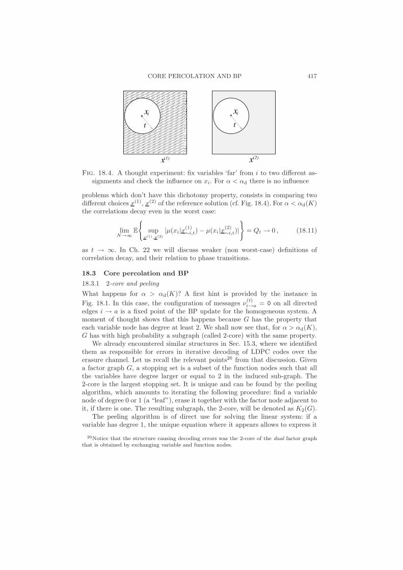
Fig. 18.4. A thought experiment: fix variables ‘far’ from i to two different as-signments and check the influence on xi. For α < αd there is no influence
problems which don’t have this dichotomy property, consists in comparing twodifferent choices x(1), x(2) of the reference solution (cf. Fig. 18.4). For α < αd(K)the correlations decay even in the worst case:
limN→∞
E
sup
x(1),x(2)
|µ(xi|x(1)∼i,t)− µ(xi|x(2)
∼i,t)|
= Qt → 0 , (18.11)
as t → ∞. In Ch. 22 we will discuss weaker (non worst-case) definitions ofcorrelation decay, and their relation to phase transitions.
18.3 Core percolation and BP
18.3.1 2-core and peeling
What happens for α > αd(K)? A first hint is provided by the instance in
Fig. 18.1. In this case, the configuration of messages ν(t)i→a = 0 on all directed
edges i → a is a fixed point of the BP update for the homogeneous system. Amoment of thought shows that this happens because G has the property thateach variable node has degree at least 2. We shall now see that, for α > αd(K),G has with high probability a subgraph (called 2-core) with the same property.
We already encountered similar structures in Sec. 15.3, where we identifiedthem as responsible for errors in iterative decoding of LDPC codes over theerasure channel. Let us recall the relevant points26 from that discussion. Givena factor graph G, a stopping set is a subset of the function nodes such that allthe variables have degree larger or equal to 2 in the induced sub-graph. The2-core is the largest stopping set. It is unique and can be found by the peelingalgorithm, which amounts to iterating the following procedure: find a variablenode of degree 0 or 1 (a “leaf”), erase it together with the factor node adjacent toit, if there is one. The resulting subgraph, the 2-core, will be denoted as K2(G).
The peeling algorithm is of direct use for solving the linear system: if avariable has degree 1, the unique equation where it appears allows to express it
26Notice that the structure causing decoding errors was the 2-core of the dual factor graphthat is obtained by exchanging variable and function nodes.

418 LINEAR EQUATIONS WITH BOOLEAN VARIABLES
in terms of other variables. It can thus be eliminated from the problem. The 2-core of G is the factor graph associated to the linear system obtained by iteratingthis procedure, which we shall refer to as the “core system”. The original systemhas a solution if and only if the core does. We shall refer to solutions of the coresystem as to core solutions.
18.3.2 Clusters
Core solutions play an important role as the set of solutions can be partitionedaccording to their core values. Given an assignment x, denote by π∗(x) its pro-jection onto the core, i.e. the vector of those entries in x that corresponds tovertices in the core. Suppose that the factor graph has a non-trivial 2-core, andlet x(∗) be a core solution. We define the cluster associated with x(∗) as the setof solutions to the linear system such that π∗(x) =ux(∗) (the reason for the name cluster will become clear in Sec. 18.5). If the coreof G is empty, we shall adopt the convention that the entire set of solutions formsa unique cluster.
Given a solution x(∗) of the core linear system, we shall denote the corre-sponding cluster as S(x(∗)). One can obtain the solutions in S(x(∗)) by runningthe peeling algorithm in the reverse direction, starting from x(∗). In this pro-cess one finds variable which are uniquely determined by x(∗), they form whatis called the ‘backbone’ of the graph. More precisely, we define the backboneB(G) as the sub-graph of G that is obtained augmenting K2(G) as follows. SetB0(G) = K2(G). For any t ≥ 0, pick a function node a which is not in Bt(G)and which has at least K − 1 of its neighboring variable nodes in Bt(G), andbuild Bt+1(G) by adding a (and its neighborhing variables) to Bt(G). If no suchfunction node exists, set B(G) = Bt(G) and halt the procedure. This definitionof B(G) does not depend on the order in which function nodes are added. Thebackbone contains the 2-core, and is such that any two solutions of the linearsystem which belong to the same cluster, coincide on the backbone.
We have thus found that the variables in a linear system naturally divide intothree possible types: The variables in the 2-core K2(G), those in B(G) \ K2(G)which are not in the core but are fixed by the core solution, and the variableswhich are not uniquely determined by x(∗). This distinction is based on thegeometry of the factor graph, i.e. it depends only the matrix H, and not on thevalue of the right hand side b in the linear system. We shall now see how BPfinds these structures.
18.3.3 Core, backbone, and belief propagation
Consider the homogeneous linear system Hx = 0, and run BP with initial con-
dition ν(0)i→a = 0. Denote by νi→a, νa→i the fixed point reached by BP (with
measure µ0) under this initialization (the reader is invited to show that such afixed point is indeed reached after a number of iterations at most equal to thenumber of messages).
The fixed point messages νi→a, νa→i can be exploited to find the 2-core

THE SAT-UNSAT THRESHOLD IN RANDOM XORSAT 419
c 1
2
34 a
b
Fig. 18.5. The factor graph of a XORSAT problem, its core (central dash-dottedpart) and its backbone (adding one function node and one variable on theright - dashed zone)
K2(G), using the following properties (which can be proved by induction overt): (i) νi→a = νa→i = 0 for each edge (i, a) in K2(G). (ii) A variable i belongsto the core K2(G) if and only if it receives messages νa→i = 0 from at least twoof the neighboring function nodes a ∈ ∂i. (iii) If a function node a ∈ 1, . . . , Mhas νi→a = 0 for all the neighboring variable nodes i ∈ ∂a, then a ∈ K2(G).
The fixed point BP messages also contain information on the backbone: avariable i belongs to the backbone B(G) if and only if it receives at least onemessage νa→i = 0 from its neighboring function nodes a ∈ ∂i.
Exercise 18.8 Consider a XORSAT problem described by the factor graph ofFig. 18.5.
(a) Using the peeling and backbone construction algorithms, check that thecore and backbone are those described in the caption.
(b) Compute the BP messages found for the homogeneous problem as a fixedpoint of BP iteration starting from the all 0 configuration. Check the coreand backbone that you obtain from these messages.
(c) Consider the general inhomogeneous linear system with the same factorgraph. Show that there exist two solutions to the core system: x1 =0, x2 = bb ⊕ bc, x3 = ba ⊕ bb ⊕ bc, x4 = ba ⊕ bb and x1 = 0, x2 = bb ⊕ bc ⊕1, x3 = ba⊕bb⊕bc, x4 = ba⊕bb⊕1. Identify the two clusters of solutions.
18.4 The SAT-UNSAT threshold in random XORSAT
We shall now see how a sharp characterization of the core size in random linearsystems provides the clue to the determination of the satisfiability threshold.Remarkably, this characterization can again be achieved through an analysis ofBP.

420 LINEAR EQUATIONS WITH BOOLEAN VARIABLES
18.4.1 The size of the core
Consider an homogeneous linear system over N variables drawn from the random
K-XORSAT ensemble, and let ν(t)i→a denote the BP messages obtained from
the initialization ν(0)i→a = 0. The density evolution analysis of Sec. 18.2.1 implies
that the fraction of edges carrying a message 0 at time t, (we called it Qt) satisfiesthe recursion equation (18.7). This recursion holds for any given t asymptoticallyas N →∞.
It follows from the same analysis that, in the large N limit, the messages
ν(t)a→i entering a variable node i are i.i.d. with Pν(t)
a→i = 0 = Qt ≡ QK−1t . Let
us for a moment assume that the limits t → ∞ and N → ∞ can be exchangedwithout much harm. This means that the fixed point messages νa→i entering avariable node i are asymptotically i.i.d. with Pνa→i = 0 = Q ≡ QK−1, whereQ is the largest solution of the fixed point equation:
Q = 1 − exp−KαQ , Q = QK−1 . (18.12)
The number of incoming messages with νa→i = 0 converges therefore to a Poissonrandom variable with mean KαQ. The expected number of variable nodes in thecore will be E|K2(G)| = NV (α, K) + o(N), where V (α, K) is the probabilitythat such a Poisson random variable is larger or equal to 2, that is
V (α, K) = 1 − e−Kα bQ −KαQ e−Kα bQ . (18.13)
In Fig. 18.6 we plot V (α) as a function of α. For α < αd(K) the peeling algorithmerases the whole graph, there is no core. The size of the core jumps to some finitevalue at αd(K) and when α →∞ the core is the full graph.
Is K2(G) a random factor graph or does it have any particular structure?By construction it cannot contain variable nodes of degree zero or one. Its ex-pected degree profile (expected fraction of nodes of any given degree) will beasymptotically Λ ≡ Λl, where Λl is the probability that a Poisson randomvariable of parameter KαQ, conditioned to be at least 2, is equal to l. ExplicitlyΛ0 = Λ1 = 0, and
Λl =1
eKα bQ − 1 −KαQ
1
l!(KαQ)l for l ≥ 2. (18.14)
Somewhat surprisingly K2(G) does not have any more structure than the onedetermined by its degree profile. This fact is stated more formally in the followingtheorem.
Theorem 18.1 Consider a factor graph G from the GN(K, Nα) ensemble withK ≥ 3. Then
(i) K2(G) = ∅ with high probability for α < αd(K).(ii) For α > αd(K), |K2(G)| = NV (α, K) + o(N) with high probability.
(iii) The fraction of vertices of degree l in K2(G) is between Λl − ε and Λl + εwith probability greater than 1 − e−Θ(N).

THE SAT-UNSAT THRESHOLD IN RANDOM XORSAT 421
-0.1
0.0
0.1
0.2
0.3
0.4
0.5
0.6
0.7
0.8
0.70 0.75 0.80 0.85 0.90 0.95 1.00α
αd αs
V (α)
C(α)
Σ(α)
Fig. 18.6. The core of random 3-XORSAT formulae contains NV (α) variables,and NC(α) equations. These numbers are plotted versus the number of equa-tions per variable of the original formula α. The number of solutions to theXORSAT linear system is Σ(α) = V (α)−C(α). The core appears for α ≥ αd,and the system becomes UNSAT for α > αs, where αs is determined byΣ(αs) = 0.
(iv) Conditionally on the number of variable nodes n = |K2(G)|, the degreeprofile being Λ, K2(G) is distributed according to the Dn(Λ, xK) ensemble.
We will not provide the proof of this theorem. The main ideas have alreadybeen presented in the previous pages, except for one important mathematicalpoint: how to exchange the limits N → ∞ and t → ∞. The basic idea is to runBP for a large but fixed number of steps t. At this point the resulting graph is‘almost’ a 2-core, and one can show that a sequential peeling procedure stops inless than Nε steps.
In Fig. 18.7 we compare the statement in this Theorem with numerical sim-ulations. The probability that G contains a 2 core Pcore(α) increases from 0 to 1as α ranges from 0 to ∞, with a threshold becoming sharper and sharper as thesize N increases. The threshold behavior can be accurately described using finitesize scaling. Setting α = αd(K) + β(K) z N−1/2 + δ(K)N−2/3 (with properlychosen β(K) and δ(K)) one can show that Pcore(α) approaches a K-independentnon-trivial limit that depends smoothly on z.
18.4.2 The threshold
Knowing that the core is a random graph with degree distribution Λl, we cancompute the expected number of equations in the core. This is given by the num-ber of vertices times their average degree, divided by K, which yields NC(α, K)+o(N) where

422 LINEAR EQUATIONS WITH BOOLEAN VARIABLES
0
0.2
0.4
0.6
0.8
1
0.6 0.7 0.8 0.9 1
100200300400600
0
0.2
0.4
0.6
0.8
1
-3 -2 -1 0 1 2 3
100200300400600
zα
Pcore Pcore
Fig. 18.7. Probability that a random graph from the GN(K,α) ensemble withK = 3 (equivalently, the factor graph of a random 3-XORSAT formula) con-tains a 2 core. On the left, the outcome of numerical simulations is comparedwith the asymptotic threshold αd(K). On the right, scaling plot (see text).
C(α, K) = αQ(1 − e−Kα bQ) . (18.15)
In Fig. 18.6 we plot C(α, K) versus α. If α < αd(K) there is no core. Forα ∈]αd,αs[ the number of equations in the core is smaller than the number ofvariables V (α, K). Above αc there are more equations than variables.
A linear system has a solution if and only if the associated core problemhas a solution. In a large random XORSAT instance, the core system involvesapproximately NC(α, K) equations between NV (α, K) variables. We shall showthat these equations are, with high probability, linearly independent as long asC(α, K) < V (α, K), which implies the following result
Theorem 18.2. (XORSAT satisfiability threshold.) For K ≥ 3, let
Σ(K,α) = V (K,α) − C(K,α) = Q− αQ(1 + (K − 1)(1 −Q)) , (18.16)
where Q, Q are the largest solution of Eq. (18.12). Let αs(K) = infα : Σ(K,α) <0. Consider a random K-XORSAT linear system with N variables and Nαequations. The following results hold with a probability going to 1 in the large Nlimit:
(i) The system has a solution when α < αs(K).(ii) It has no solution when α > αs(K).(iii) For α < αs(K) the number of solutions is 2N(1−α)+o(N), and the number
of clusters is 2NΣ(K,α)+o(N).
Notice that the the last expression in Eq. (18.16) is obtained from Eqs. (18.13)and (18.15) using the fixed point condition (18.12).
The prediction of this theorem is compared with numerical simulations inFig. 18.8, while Fig. 18.9 summarizes the results on the thresholds for XORSAT.Proof: We shall convey the basic ideas of the proof and refer to the literaturefor technical details.

THE SAT-UNSAT THRESHOLD IN RANDOM XORSAT 423
0
0.2
0.4
0.6
0.8
1
0.2 0.4 0.6 0.8 1 1.2 1.4 1.6 1.8
50100200400
αs(3)
α
Psat
Fig. 18.8. Probability that a random 3-XORSAT formula with N variables andNα equations is SAT, estimated numerically by generating 103÷104 randominstances.
K 3 4 5αd 0.81847 0.77228 0.70178αs 0.91794 0.97677 0.99244
0 αd αs
Fig. 18.9. Left: A pictorial view of the phase transitions in random XORSATsystems. The satisfiability threshold is αs. In the ‘Easy-SAT’ phase α < αd
there is a single cluster of solutions. In the ‘Hard-SAT’ phase αd < α < αs
the solutions of the linear system are grouped in well separated clusters.Right: The thresholds αd, αs for various values of K. At large K one has:αd(K) 1 log K/K and αs(K) = 1 − e−K + O(e−2K).
Let us start by proving (ii), namely that for α > αs(K) random XORSATinstances are with high probability UNSAT. This follows from a linear algebraargument. Let H∗ denote the 0−1 matrix associated with the core, i.e. the matrixincluding those rows/columns such that the associated function/variable nodesbelong to K2(G). Notice that if a given row is included in H∗ then all the columnscorresponding to non-zero entries of that row are also in H∗. As a consequence,a necessary condition for the rows of H to be independent is that the rows of H∗are independent. This is in turn impossible if the number of columns in H∗ issmaller than its number of rows.
Quantitatively, one can show that M − rank(H) ≥ rows(H∗)− cols(H∗) (withthe obvious meanings of rows( · ) and cols( · )). In large random XORSAT sys-tems, Theorem 18.1 implies that rows(H∗)−cols(H∗) = −NΣ(K,α)+o(N) with

424 LINEAR EQUATIONS WITH BOOLEAN VARIABLES
Fig. 18.10. Adding a function nodes involving a variable node of degree one.The corresponding linear equation is independent from the other ones.
high probability. According to our discussion in Sec. 18.1.1, among the 2M pos-sible choices of the right-hand side vector b, only 2rank(H) are in the image of H
and thus lead to a solvable system. In other words, conditional on H, the prob-ability that random XORSAT is solvable is 2rank(H)−M . By the above argumentthis is, with high probability, smaller than 2NΣ(K,α)+o(N). Since Σ(K,α) < 0 forα > αs(K), it follows that the system is UNSAT with high probability.
In order to show that a random system is satisfiable with high probabilitywhen α < αs(K), one has to prove the following facts: (i) if the core matrix H∗has maximum rank, then H has maximum rank as well; (ii) if α < αs(K), thenH∗ has maximum rank with high probability. As a byproduct, the number ofsolutions is 2N−rank(H) = 2N−M .
(i) The first step follows from the observation that G can be constructed fromK2(G) through an inverse peeling procedure. At each step one adds a functionnode which involves at least a degree one variable (see Fig. 18.10). Obviously thisnewly added equation is linearly independent of the previous ones, and thereforerank(H) = rank(H∗) + M − rows(H∗).
(ii) Let n = cols(H∗) be the number of variable nodes and m = rows(H∗) thenumber of function nodes in the core K2(G). Let us consider the homogeneoussystem on the core, H∗x = 0, and denote by Z∗ the number of solutions to thissystem. We will show that with high probability this number is equal to 2n−m.This means that the dimension of the kernel of H∗ is n − m and therefore H∗has full rank.
We know from linear algebra that Z∗ ≥ 2n−m. To prove the reverse inequal-ity we use a first moment method. According to Theorem 18.1, the core is auniformly random factor graph with n = NV (K,α) + o(N) variables and de-gree profile Λ = Λ + o(1). Denote by E the expectation value with respect tothis ensemble. We shall use below a first moment analysis to show that, whenα < αc(K):
E Z∗ = 2n−m[1 + oN (1)] . (18.17)

THE SAT-UNSAT THRESHOLD IN RANDOM XORSAT 425
-0.04
-0.02
0.00
0.02
0.04
0.06
0.0 0.1 0.2 0.3 0.4-0.04
-0.02
0.00
0.02
0.04
0.06
0.0 0.1 0.2 0.3 0.4-0.04
-0.02
0.00
0.02
0.04
0.06
0.0 0.1 0.2 0.3 0.4-0.04
-0.02
0.00
0.02
0.04
0.06
0.0 0.1 0.2 0.3 0.4-0.04
-0.02
0.00
0.02
0.04
0.06
0.0 0.1 0.2 0.3 0.4-0.04
-0.02
0.00
0.02
0.04
0.06
0.0 0.1 0.2 0.3 0.4
ω
φ(ω)
Fig. 18.11. The exponential rate φ(ω) of the weight enumerator of the core ofa random 3-XORSAT formula. From top to bottom α = αd(3) ≈ 0.818469,0.85, 0.88, 0.91, and 0.94 (recall that αs(3) ≈ 0.917935). Inset: blow up ofthe small ω region.
Then Markov inequality PZ∗ > 2n−m ≤ 2−n+mEZ∗ implies the bound.The surprise is that Eq. (18.17) holds, and thus a simple first moment esti-
mate allows to establish that H∗ has full rank. We saw in Exercise 18.6 that thesame approach, when applied directly to the original linear system, fails abovesome α∗(K) which is strictly smaller than αs(K). Reducing the original graph toits two-core has drastically reduced the fluctuations of the number of solutions,thus allowing for a successful application of the first moment method.
We now turn to the proof of Eq. (18.17), and we shall limit ourselves to thecomputation of EZ∗ to the leading exponential order, when the core size anddegree profiles take their typical values n = NV (K,α), Λ = Λ and P (x) = xK .This problem is equivalent to computing the expected number of codewords inthe LDPC code defined by the core system, which we already did in Sec. 11.2.The result takes the typical form
EZ∗.= exp
N sup
ω∈[0,V (K,α)]φ(ω)
. (18.18)
Here φ(ω) is the exponential rate for the number of solutions with weight Nω.Adapting Eq. (11.18) to the present case, we obtain the parametric expression:
φ(ω) = −ω log x − η(1 − e−η) log(1 + yz) + (18.19)
+∑
l≥2
e−ηηl
l!log(1 + xyl) +
η
K(1 − e−η) log qK(z) ,
ω =∑
l≥2
e−ηηl
l!
xyl
1 + xyl. (18.20)

426 LINEAR EQUATIONS WITH BOOLEAN VARIABLES
where η = KαQ∗, qK(z) = [(1 + z)K + (1 − z)K ]/2 and y = y(x), z = z(x) arethe solution of
z =
∑l≥1[η
l/l!] [xyl−1/(1 + xyl)]∑
l≥1[ηl/l!] [1/(1 + xyl)]
, y =(1 + z)K−1 − (1 − z)K−1
(1 + z)K−1 + (1 − z)K−1. (18.21)
With a little work one sees that ω∗ = V (K,α)/2 is a local maximum of φ(ω),with φ(ω∗) = Σ(K,α) log 2. As long as ω∗ is a global maximum, EZ∗|n,Λ .
=expNφ(ω∗)
.= 2n−m. It turns out, cf. Fig. 18.11, that the only other local
maximum is at ω = 0 corresponding to φ(0) = 0. Therefore EZ∗|n,Λ .= 2n−m
as long as φ(ω∗) = Σ(K,α) > 0, i.e. for any α < αs(K)Notice that the actual proof of Eq. (18.17) is more complicate because it
requires estimating the sub-exponential factors. Nevertheless it can be carriedout successfully. !
18.5 The Hard-SAT phase: clusters of solutions
In random XORSAT, the whole regime α < αs(K) is SAT. This means that,with high probability there exist solutions to the random linear system, and thenumber of solutions is in fact Z
.= eN(1−α). Notice that the number of solutions
does not present any precursor of the SAT-UNSAT transition at αs(K) (recallthat αs(K) < 1), nor does it carry any trace of the sudden appearence of anon-empty two core at αd(K).
On the other hand the threshold αd(K) separates two phases, that we will call‘Easy-SAT’ (for α < αd(K)) and ‘Hard-SAT’ phase (for α ∈]αd(K),αs(K)[).These two phases differ in the structure of the solution space, as well as in thebehavior of some simple algorithms.
In the Easy-SAT phase there is no core, solutions can be found in (expected)linear time using the peeling algorithm and they form a unique cluster. In theHard-SAT the factor graph has a large 2-core, and no algorithm is known thatfinds a solution in linear time. Solutions are partitioned in 2NΣ(K,α)+o(N) clusters.Until now the name ‘cluster’ has been pretty arbitrary, and only denoted a subsetof solutions that coincide in the core. The next result shows that distinct clustersare ‘far apart’ in Hamming space.
Proposition 18.3 In the Hard-SAT phase there exists δ(K,α) > 0 such that,with high probability, any two solutions in distinct clusters have Hamming dis-tance larger than Nδ(K,α).
Proof: The proof follows from the computation of the weight enumerator expo-nent φ(ω), cf. Eq. (18.20) and Fig. 18.11. One can see that for any α > αd(K),φ′(0) < 0, and, as a consequence there exists δ(K,α) > 0 such that φ(ω) < 0for 0 < ω < δ(K,α). This implies that if x∗, x′
∗ are two distinct solution of thecore linear system, then either d(x∗, x
′∗) = o(N) or d(x, x′) > Nδ(K,α). It turns
out that the first case can be excluded along the lines of the minimal distancecalculation of Sec. 11.2. Therefore, if x, x′ are two solutions belonging to distinctclusters d(x, x′) ≥ d(π∗(x),π∗(x′)) ≥ Nδ(K,α). !

AN ALTERNATIVE APPROACH: THE CAVITY METHOD 427
This result suggests to regard clusters as ‘lumps’ of solutions well separatedfrom each other. One aspect which is conjectured, but not proved, concerns thefact that clusters form ‘well connected components.’ By this we mean that anytwo solutions in the a cluster can be joined by a sequence of other solutions,whereby two successive solutions in the sequence differ in at most sN variables,with sN = o(N) (a reasonable expectation is sN = Θ(log N)).
18.6 An alternative approach: the cavity method
The analysis of random XORSAT in the previous sections relied heavily on thelinear structure of the problem, as well as on the very simple instance distribu-tion. This section describes an alternative approach that is potentially generaliz-able to more complex situations. The price to pay is that this second derivationrelies on some assumptions on the structure of the solution space. The observa-tion that our final results coincide with the ones obtained in the previous sectiongives some credibility to these assumptions.
The starting point is the remark that BP correctly computes the marginals ofµ( · ) (the uniform measure over the solution space) for α < αd(K), i.e. as long asthe set of solutions forms a single cluster. We want to extend its domain of validityto α > αd(K). If we index by n ∈ 1, . . . ,N the clusters, the uniform measureµ( · ) can be decomposed into the convex combination of uniform measures overeach single cluster:
µ( · ) =N∑
n=1
wn µn( · ) . (18.22)
Notice that in the present case wn = 1/N is independent of n and the measuresµn( · ) are obtained from each other via a translation, but this will not be truein more general situations.
Consider an inhomogeneous XORSAT linear system and denote by x(∗) oneof its solutions in cluster n. The distribution µn has single variable marginals
µn(xi) = I(xi = x(∗)i ) if node i belongs to the backbone, and µn(xi = 0) =
µn(xi = 1) = 1/2 on the other nodes.In fact we can associate to each solution x(∗) a fixed point of the BP equation.
We already described this in Section 18.2.1, cf. Eq. (18.9). On this fixed point
messages take one of the following three values: ν(∗)i→a(xi) = I(xi = 0) (that we
will denote as ν(∗)i→a = 0), ν(∗)
i→a(xi) = I(xi = 1) (denoted ν(∗)i→a = 1), ν(∗)
i→a(xi =
0) = ν(∗)i→a(xi = 1) = 1/2 (denoted ν(∗)
i→a = ∗). Analogous notations hold forfunction-to-variable node messages. The solution can be written most easily interms of the latter
ν(∗)a→i =
1 if x(∗)i = 1 and i, a ∈ B(G),
0 if x(∗)i = 0 and i, a ∈ B(G),
∗ otherwise.
(18.23)

428 LINEAR EQUATIONS WITH BOOLEAN VARIABLES
Notice that these messages only depend on the value of x(∗)i on the backbone of
G, hence they depend on x(∗) only through the cluster it belongs to. Reciprocally,for any two distinct clusters, the above definition gives two distinct fixed points.
Because of this remark we shall denote these fixed points as ν(n)i→a, ν(n)
a→i, wheren is a cluster index.
Let us recall the BP fixed point condition:
νi→a =
∗ if νb→i = ∗ for all b ∈ ∂i\a,any ‘non ∗’ νb→i otherwise.
(18.24)
νa→i =
∗ if ∃j ∈ ∂a\i s.t. νj→a = ∗,ba ⊕ νj1→a ⊕ · · ·⊕ νjl→a otherwise.
(18.25)
Below we shall denote symbolically these equations as
νi→a = fνb→i , νa→i = fνj→a . (18.26)
Let us summarize our findings.
Proposition 18.4 To each cluster n we can associate a distinct fixed point of
the BP equations (18.25) ν(n)i→a, ν(n)
a→i, such that ν(n)a→i ∈ 0, 1 if i, a are in the
backbone and ν(n)a→i = ∗ otherwise.
Note that the converse of this proposition is false: there may exist solutions tothe BP equations which are not of the previous type. One of them is the all ∗solution. Nontrivial solutions exist as well as shown in Fig. 18.12.
An introduction to the 1RSB cavity method in the general case will be pre-sented in Ch. 19. Here we give a short informal preview in the special case of theXORSAT: the reader will find a more formal presentation in the next chapter.The first two assumptions of the 1RSB cavity method can be summarized asfollows (all statements are understood to hold with high probability).
Assumption 1 In a large random XORSAT instance, for each cluster ‘n’ ofsolutions, the BP solution ν(n), ν(n) provides an accurate ‘local’ description ofthe measure µn( · ).
This means that for instance the one point marginals are given by µn(xj) ∼=∏a∈∂j ν(n)
a→j(xj) + o(1), but also that local marginals inside any finite cavity arewell approximated by formula (14.18).
Assumption 2 For a large random XORSAT instance in the Hard-SAT phase,the number of clusters eNΣ is exponential in the number of variables. Further, thenumber of solutions of the BP equations (18.25) is, to the leading exponentialorder, the same as the number of clusters. In particular it is the same as thenumber of solutions constructed in Proposition 18.4.
A priori one might have hoped to identify the set of messages ν(n)i→a for
each cluster. The cavity method gives up this ambitious objective and aims to

AN ALTERNATIVE APPROACH: THE CAVITY METHOD 429
corefrozen
1
2
a
b
Fig. 18.12. Left: A set of BP messages associated with one cluster (clusternumber n) of solutions. An arrow along an edge means that the correspond-
ing message (either ν(n)i→a or ν(n)
a→i) takes value in 0, 1. The other messagesare equal to ∗. Right: A small XORSAT instance. The core is the wholegraph. In the homogeneous problem there are two solutions, which formtwo clusters: x1 = x2 = 0 and x1 = x2 = 1. Beside the two correspond-ing BP fixed points described in Proposition 18.4, and the all-∗ fixed point,there exist other fixed points such as νa→1 = ν1→b = νb→2 = ν2→a = 0,νa→2 = ν2→b = νb→1 = ν1→a = ∗.
compute the distribution of ν(n)i→a for any fixed edge i → a, when n is a cluster
index drawn with distribution wn. We thus want to compute the quantities:
Qi→a(ν) = Pν(n)
i→a = ν
, Qa→i(ν) = Pν(n)
a→i = ν
. (18.27)
for ν, ν ∈ 0, 1, ∗. Computing these probabilities rigorously is still a challengingtask. In order to proceed, we make some assumption on the joint distribution of
the messages ν(n)i→a when n is a random cluster index (chosen from the probability
wn).The simplest idea would be to assume that messages on ‘distant’ edges are
independent. For instance let us consider the set of messages entering a givenvariable node i. Their only correlations are induced through BP equations alongthe loops to which i belongs. Since in random K-XORSAT formulae such loopshave, with high probability, length of order log N , one might think that mes-sages incoming a given node are asymptotically independent. Unfortunatelythis assumption is false. The reason is easily understood if we assume thatQa→i(0), Qa→i(1) > 0 for at least two of the function nodes a adjacent to a

430 LINEAR EQUATIONS WITH BOOLEAN VARIABLES
given variable node i. This would imply that, with positive probability a ran-
domy sampled cluster has ν(n)a→i = 0, and ν(n)
b→i = 1. But there does not exist anysuch cluster, because in such a situation there is no consistent prescription forthe marginal distribution of xi under µn( · ).
Our assumption will be that the next simplest thing happens: messages areindependent conditional to the fact that they do not contradict each other.
Assumption 3 Consider the Hard-SAT phase of a random XORSAT problem.Denote by i ∈ G a uniformly random node, by n a random cluster index with
distribution wn, and let - be an integer ≥ 1. Then the messages ν(n)j→b, where
(j, b) are all the edges at distance - from i and directed towards i, are asymptot-ically independent under the condition of being compatible.
Here ‘compatible’ means the following. Consider the linear system Hi,%xi,% =0 for the neighborhood of radius - around node i. If this admits a solution underthe boundary condition xj = νj→b for all the boundary edges (j, b) on whichνj→b ∈ 0, 1, then the messages νj→b are said to be compatible.
Given the messages νj→b at the boundary of a radius-- neighborhood, theBP equations (18.24) and (18.25) allow to determine the messages inside thisneighborhood. Consider in particular two nested neighborhoods at distance -and - + 1 from i. The inwards messages on the boundary of the largest neigh-borhood completely determines the ones on the boundary of the smallest one. Alittle thought shows that, if the messages on the outer boundary are distributedaccording to Assumption 3, then the distribution of the resulting messages on theinner boundary also satisfies the same assumption. Further, the distributions areconsistent if and only if the following ‘survey propagation’ equations are satisfiedby the one-message marginals:
Qi→a(ν) ∼=∑
bνb
∏
b∈∂i\a
Qb→i(νb) I(ν = fνb) I(νbb∈∂i\a ∈ COMP) , (18.28)
Qa→i(ν) =∑
νj
∏
j∈∂a\i
Qj→a(νj) I(ν = fνj) . (18.29)
Here and νb ∈ COMP only if the messages are compatible (i.e. they do notcontain both a 0 and a 1). Since Assumptions 1, 2, 3 above hold only withhigh probability and asymptotically in the system size, the equalities in (18.28),(18.29) must also be interpreted as approximate. The equations should be satis-fied within any given accuracy ε, with high probability as N → ∞.

AN ALTERNATIVE APPROACH: THE CAVITY METHOD 431
Exercise 18.9 Show that Eqs. (18.28), (18.29) can be written explicitly as
Qi→a(0) ∼=∏
b∈∂i\a
(Qb→i(0) + Qb→i(∗)) −∏
b∈∂i\a
Qb→i(∗) , (18.30)
Qi→a(1) ∼=∏
b∈∂i\a
(Qb→i(1) + Qb→i(∗)) −∏
b∈∂i\a
Qb→i(∗) (18.31)
Qi→a(∗) ∼=∏
b∈∂i\a
Qb→i(∗) , (18.32)
where the ∼= symbol hides a global normalization constant, and
Qa→i(0) =1
2
∏
j∈∂a\i
(Qj→a(0) + Qj→a(1)) +∏
j∈∂a\i
(Qj→a(0) −Qj→a(1))
,
(18.33)
Qa→i(1) =1
2
∏
j∈∂a\i
(Qj→a(0) + Qj→a(1)) −∏
j∈∂a\i
(Qj→a(0) −Qj→a(1))
,
(18.34)
Qa→i(∗) = 1 −∏
j∈∂a\i
(Qj→a(0) + Qj→a(1)) . (18.35)
The final step of the 1RSB cavity method consists in looking for a solution ofEqs. (18.28), (18.29). There are no rigorous results on the existence or number ofsuch solutions. Further, since these equations are only approximate, approximatesolutions should be considered as well. In the present case a very simple (andsomewhat degenerate) solution can be found that yields the correct predictionsfor all the quantities of interest. In this solution, the message distributions takeone of two possible forms: on some edges one has Qi→a(0) = Qi→a(1) = 1/2(with an abuse of notation we shall write Qi→a = 0 in this case), on some otheredges Qi→a(∗) = 1 (we will then write Qi→a = ∗). Analogous forms hold forQa→i. A little algebra shows that this is a solution if and only if the η’s satisfy
Qi→a =
∗ if Qb→i = ∗ for all b ∈ ∂i\a,0 otherwise.
(18.36)
Qa→i =
∗ if ∃j ∈ ∂a\i s.t. Qj→a = ∗,0 otherwise.
(18.37)
These equations are identical to the original BP equations for the homogeneousproblem (this feature is very specific to XORSAT and will not generalize tomore advanced applications of the method). However the interpretation is now

432 LINEAR EQUATIONS WITH BOOLEAN VARIABLES
completely different. On the edges where Qi→a = 0 the corresponding message
ν(n)i→a depend on the cluster n and ν(n)
i→a = 0 (respectively = 1) in half of theclusters. These edges are those inside the core, or in the backbone but directed‘outward’ with respect to the core, as shown in Fig.18.12. On the other edges,
the message does not depend upon the cluster and ν(n)i→a = ∗ for all n’s.
A concrete interpretation of these results is obtained if we consider the onebit marginals µn(xi) under the single cluster measure. According to Assumption
1 above, we have µn(xi = 0) = µn(xi = 1) = 1/2 if ν(n)a→i = ∗ for all a ∈ ∂i.
If on the other hand ν(n)a→i = 0 (respectively = 1) for at least one a ∈ ∂i, then
µn(xi = 0) = 1 (respectively µn(xi = 0) = 0). We thus recover the full solutiondiscussed in the previous sections: inside a given cluster n, the variables in thebackbone are completely frozen, either to 0 or to 1. The other variables haveequal probability to be 0 or 1 under the measure µn.
The cavity approach allows to compute the complexity Σ(K,α) as well asmany other properties of the measure µ( · ). We will see this in the next chapter.
Notes
Random XORSAT formulae were first studied as a simple example of randomsatisfiability in (Creignou and Daude, 1999). This work considered the case of‘dense formulae’ where each clause includes O(N) variables. In this case the SAT-UNSAT threshold is at α = 1. In coding theory this model had been characterizedsince the work of Elias in the fifties (Elias, 1955), cf. Ch. 6.
The case of sparse formulae was addressed using moment bounds in (Creignou,Daude and Dubois, 2003). The replica method was used in (Ricci-Tersenghi,Weigt and Zecchina, 2001; Franz, Leone, Ricci-Tersenghi and Zecchina, 2001a;Franz, Mezard, Ricci-Tersenghi, Weigt and Zecchina, 2001b) to derive the clus-tering picture, determine the SAT-UNSAT threshold, and study the glassy prop-erties of the clustered phase.
The fact that, after reducing the linear system to its core, the first momentmethod provides a sharp characterization of the SAT-UNSAT threshold was dis-covered independently by two groups: (Cocco, Dubois, Mandler and Monasson,2003) and (Mezard, Ricci-Tersenghi and Zecchina, 2003). The latter also dis-cusses the application of the cavity method to the problem. The full secondmoment calculation that completes the proof can be found for the case K = 3in (Dubois and Mandler, 2002).
The papers (Montanari and Semerjian, 2005; Montanari and Semerjian, 2006a;Mora and Mezard, 2006) were devoted to finer geometrical properties of the setof solutions of random K-XORSAT formulae. Despite these efforts, it remainsto be proved that clusters of solutions are indeed ‘well connected.’
Since the locations of various transitions are known rigorously, a naturalquestion is to study the critical window. Finite size scaling of the SAT-UNSATtransition was investigated numerically in (Leone, Ricci-Tersenghi and Zecchina,2001). A sharp characterization of finite-size scaling for the appearence of a 2-

NOTES 433
core, corresponding to the clustering transition, was achieved in (Dembo andMontanari, 2008a).
19
THE 1RSB CAVITY METHOD
The effectiveness of belief propagation depends on one basic assumption: whena function node is pruned from the factor graph, the adjacent variables becomeweakly correlated with respect to the resulting distribution. This hypothesis maybreak down either because of the existence of small loops in the factor graph,or because variables are correlated on large distances. In factor graphs with alocally tree-like structure, the second scenario is responsible for the failure ofBP. The emergence of such long range correlations is a signature of a phasetransition separating a ‘weakly correlated’ and a ‘highly correlated’ phase. Thelatter is often characterized by the decomposition of the (Boltzmann) probabilitydistribution into well separated ‘lumps’ (pure Gibbs states).
We considered a simple example of this phenomenon in our study of randomXORSAT. A similar scenario holds in a variety of problems from random graphcoloring to random satisfiability and spin glasses. The reader should be warnedthat the structure and organization of pure states in such systems is far frombeing fully understood. Furthermore, the connection between long range correla-tions and pure states decomposition is more subtle than suggested by the aboveremarks.
Despite these complications, physicists have developed a non-rigorous ap-proach to deal with this phenomenon: the “one step replica symmetry breaking”(1RSB) cavity method. The method postulates a few properties of the pure statedecomposition, and, on this basis, allows to derive a number of quantitative pre-dictions (‘conjectures’ from a mathematics point of view). Examples include thesatisfiability threshold for random K-SAT and other random constraint satisfac-tion problems.
The method is rich enough to allow for some self-consistency checks of suchassumptions. In several cases in which the 1RSB cavity method passed this test,its predictions have been confirmed by rigorous arguments (and there is no casein which they have been falsified so far). These successes encourage the quest fora mathematical theory of Gibbs states on sparse random graphs.
This chapter explains the 1RSB cavity method. It alternates between ageneral presentation and a concrete illustration on the XORSAT problem. Westrongly encourage the reader to read the previous chapter on XORSAT beforethe present one. This should help her to gain some intuition of the whole scenario.
We start with a general description of the 1RSB glass phase, and the de-composition in pure states, in Sec. 19.1. Section 19.2 introduces an auxiliaryconstraint satisfaction problem to count the number of solutions of BP equa-tions. The 1RSB analysis amounts to applying belief propagation to this auxil-
434

BEYOND BP: MANY STATES 435
iary problem. One can then apply the methods of Ch. 14 (for instance, densityevolution) to the auxiliary problem. Section 19.3 illustrates the approach on theXORSAT problem and shows how the 1RSB cavity method recovers the rigorousresults of the previous chapter.
In Sec. 19.4 we show how the 1RSB formalism, which in general is rathercomplicated, simplifies considerably when the temperature of the auxiliary con-straint satisfaction problem takes the value x = 1. Section 19.5 explains how toapply it to optimization problems (leveraging on the min-sum algorithm) lead-ing to the Survey Propagation algorithm. The concluding section 19.6 describesthe physical intuition which underlies the whole method. The appendix 19.6.3contains some technical aspects of the survey propagation equations applied toXORSAT, and their statistical analysis.
19.1 Beyond BP: many states
19.1.1 Bethe measures
The main lesson of the previous chapters is that in many cases, the probabilitydistribution specified by graphical models with a locally tree-like structure takesa relatively simple form, that we shall call a Bethe measure (or Bethe state). Letus first define precisely what we mean by this, before we proceed to discuss whatkinds of other scenarios can be encountered.
As in Ch. 14, we consider a factor graph G = (V, F, E), with variable nodesV = 1, · · · , N, factor nodes F = 1, · · · , M and edges E. The joint probabil-ity distribution over the variables x = (x1, . . . , xN ) ∈ XN takes the form
µ(x) =1
Z
M∏
a=1
ψa(x∂a) . (19.1)
Given a subset of variable nodes U ⊆ V (which we shall call a ‘cavity’),the induced subgraph GU = (U, FU , EU ) is defined as the factor graph thatincludes all the factor nodes a such that ∂a ⊆ U , and the adjacent edges. We alsowrite (i, a) ∈ ∂U if i ∈ U and a ∈ F \ FU . Finally, a set of messages νa→i isa set of probability distributions over X , indexed by directed edges a → i in Ewith a ∈ F , i ∈ V .
Definition 19.1. (Informal) The probability distribution µ is a Bethe mea-sure (or Bethe state) if there exists a set of messages νa→i, such that, for‘almost all’ the ‘finite size’ cavities U , the distribution µU ( · ) of the variables inU is approximated as
µU (xU ) ∼=∏
a∈FU
ψa(x∂a)∏
(ia)∈∂U
νa→i(xi) + err(xU ) , (19.2)
where err(xU ) is a ‘small’ error term, and ∼= denotes as usual equality up to anormalization.

436 THE 1RSB CAVITY METHOD
i
aj
b
i
aj
b
Fig. 19.1. Two examples of cavities. The right hand one is obtained by addingthe extra function node a. The consistency of the Bethe measure in these twocavities implies the BP equation for νa→i, see Exercise 19.1.
A formal definition should specify what is meant by ‘almost all’, ‘finite size’ and‘small.’ This can be done by introducing a tolerance εN (with εN ↓ 0 as N →∞)and a size LN (where LN is bounded as N →∞). One then requires that somenorm of err( · ) (e.g. an Lp norm) is smaller than εN for a fraction larger than1 − εN of all possible cavities U of size |U | < LN . The underlying intuition isthat the measure µ( · ) is well approximated locally by the given set of messages.In the following we shall follow physicists’ habit of leaving implicit the variousapproximation errors.
Notice that the above definition does not make use of the fact that µ factorizesas in Eq. (19.1). It thus apply to any distribution over x = xi : i ∈ V .
If µ( · ) is a Bethe measure with respect to the message set νa→i, thenthe consistency of Eq. (19.2) for different choices of U implies some non-trivialconstraints on the messages. In particular if the loops in the factor graph G arenot too small (and under some technical condition on the functions ψa( · )) thenthe messages must be close to satisfying BP equations. More precisely, we definea quasi-solution of BP equations as a set of messages which satisfy almost allthe equations within some accuracy. The reader is invited to prove this statementin the exercise below.
BEYOND BP: MANY STATES 437
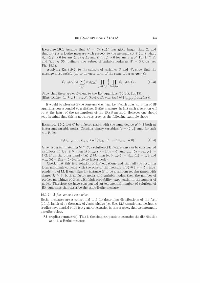
Exercise 19.1 Assume that G = (V, F, E) has girth larger than 2, andthat µ( · ) is a Bethe measure with respect to the message set νa→i whereνa→i(xi) > 0 for any (i, a) ∈ E, and ψa(x∂a) > 0 for any a ∈ F . For U ⊆ V ,and (i, a) ∈ ∂U , define a new subset of variable nodes as W = U ∪ ∂a (seeFig. 19.1).
Applying Eq. (19.2) to the subsets of variables U and W , show that themessage must satisfy (up to an error term of the same order as err( · )):
νa→i(xi) ∼=∑
x∂a\i
ψa(x∂a)∏
j∈∂a\i
∏
b∈∂j\a
νb→j(xj)
. (19.3)
Show that these are equivalent to the BP equations (14.14), (14.15).[Hint: Define, for k ∈ V , c ∈ F , (k, c) ∈ E, νk→c(xk) ∼=
∏d∈∂k\c νd→k(xk)].
It would be pleasant if the converse was true, i.e. if each quasi-solution of BPequations corresponded to a distinct Bethe measure. In fact such a relation willbe at the heart of the assumptions of the 1RSB method. However one shouldkeep in mind that this is not always true, as the following example shows:
Example 19.2 Let G be a factor graph with the same degree K ≥ 3 both atfactor and variable nodes. Consider binary variables, X = 0, 1, and, for eacha ∈ F , let
ψa(xi1(a), . . . , xiK (a)) = I(xi1(a) ⊕ · · ·⊕ xiK (a) = 0) . (19.4)
Given a perfect matching M ⊆ E, a solution of BP equations can be constructedas follows. If (i, a) ∈ M, then let νa→i(xi) = I(xi = 0) and νi→a(0) = νi→a(1) =1/2. If on the other hand (i, a) .∈ M, then let νa→i(0) = νa→i(1) = 1/2 andνi→a(0) = I(xi = 0) (variable to factor node).
Check that this is a solution of BP equations and that all the resultinglocal marginals coincide with the ones of the measure µ(x) ∼= I(x = 0), inde-pendently of M. If one takes for instance G to be a random regular graph withdegree K ≥ 3, both at factor nodes and variable nodes, then the number ofperfect matchings of G is, with high probability, exponential in the number ofnodes. Therefore we have constructed an exponential number of solutions ofBP equations that describe the same Bethe measure.
19.1.2 A few generic scenarios
Bethe measures are a conceptual tool for describing distributions of the form(19.1). Inspired by the study of glassy phases (see Sec. 12.3), statistical mechanicsstudies have singled out a few generic scenarios in this respect, that we informallydescribe below.
RS (replica symmetric). This is the simplest possible scenario: the distributionµ( · ) is a Bethe measure.

438 THE 1RSB CAVITY METHOD
A slightly more complicated situation (that we still ascribe to the ‘replicasymmetric’ family) arises when µ( · ) decomposes into a finite set of Bethemeasures related by ‘global symmetries’, as in the Ising ferromagnet dis-cussed in Sec. 17.3.
d1RSB (dynamic one-step replica symmetry breaking). There exists an exponen-tially large (in the system size N) number of Bethe measures. The measureµ decomposes into a convex combination of these Bethe measures:
µ(x) =∑
n
wn µn(x) , (19.5)
with weights wn exponentially small in N . Furthermore µ( · ) is itself aBethe measure.
s1RSB (static one-step replica symmetry breaking). As in the d1RSB case, thereexists an exponential number of Bethe measures, and µ decomposes into aconvex combination of such states. However, a finite number of the weightswn is of order 1 as N →∞, and (unlike in the previous case) µ is not itselfa Bethe measure.
In the following we shall focus on the d1RSB and s1RSB scenarios, that areparticularly interesting, and can be treated in a unified framework (we shallsometimes refer to both of them as 1RSB). More complicate scenarios, such as‘full RSB’, are also possible. We do not discuss such scenarios here because, sofar, one has a relatively poor control of them in sparse graphical models.
In order to proceed further, we shall make a series of assumptions on thestructure of Bethe states in the 1RSB case. While further research work is re-quired to formalize completely these assumptions, they are precise enough forderiving several interesting quantitative predictions.
To avoid technical complications, we assume that the compatibility functionsψa( · ) are strictly positive. (The cases with ψa( · ) = 0 should be treated as limitcases of such models). Let us index by n the various quasi-solutions νn
i→a, νna→i
of the BP equations. To each of them we can associate a Bethe measure, andwe can compute the corresponding Bethe free-entropy Fn = F(νn). The threepostulates of the 1RSB scenario are listed below.
Assumption 1 There exist exponentially many quasi-solutions of BP equations.The number of such solutions with free-entropy F(νn) ≈ Nφ is (to leading expo-nential order) expNΣ(φ), where Σ( · ) is the complexity function27 .
This can be expressed more formally as follows. There exists a function Σ : R →R+ (the complexity) such that, for any interval [φ1,φ2], the number of quasi-solutions of BP equations with F(νn) ∈ [Nφ1, Nφ2] is expNΣ∗ + o(N) whereΣ∗ = supΣ(φ) : φ1 ≤ φ ≤ φ2. We shall also assume in the following thatΣ(φ) is ‘regular enough’ without entering details.
27As we are only interested in the leading exponential behavior, the details of the definitionsof quasi-solutions become irrelevant, as long as (for instance) the fraction of violated BPequations vanishes in the large N limit.

THE 1RSB CAVITY EQUATIONS 439
Among Bethe measures, a special role is played by the ones that have shortrange correlations (are extremal). We already mentioned this point in Ch. 12,and shall discuss the relevant notion of correlation decay in Ch. 22. We denotethe set of extremal measures as E.
Assumption 2 The ‘canonical’ measure µ defined as in Eq. (19.1) can be writ-ten as a convex combination of extremal Bethe measures
µ(x) =∑
n∈E
wn µn(x) , (19.6)
with weights related to the Bethe free-entropies wn = eFn/Ξ, Ξ ≡∑
n∈EeFn.
Note that Assumption 1 characterizes the number of (approximate) BP fixedpoints, while Assumption 2 expresses the measure µ( · ) in terms of extremalBethe measures. While each such measure gives rise to a BP fixed point by thearguments in the previous Section, it is not clear that the reciprocal holds. Thenext assumption implies that this is the case, to the leading exponential order.
Assumption 3 To leading exponential order, the number of extremal Bethemeasures equals the number of quasi-solutions of BP equation: the number ofextremal Bethe measures with free-entropy ≈ Nφ is also given by expNΣ(φ).
19.2 The 1RSB cavity equations
Within the three assumptions described above, the complexity function Σ(φ)provides basic information on how the measure µ decomposes into Bethe mea-sures. Since the number of extremal Bethe measures with a given free entropydensity is exponential in the system size, it is natural to treat them within astatistical physics formalism. BP messages of the original problem will be thenew variables and Bethe measures will be the new configurations. This is what1RSB is about.
We introduce the auxiliary statistical physics problem through the definitionof a canonical distribution over extremal Bethe measures: we assign to measuren ∈ E, the probability wn(x) = exFn/Ξ(x). Here x plays the role of an inversetemperature (and is often called the Parisi 1RSB parameter) 28. The partitionfunction of this generalized problem is
Ξ(x) =∑
n∈E
exFn.=
∫eN [xφ+Σ(φ)] dφ . (19.7)
According to Assumption 2 above, extremal Bethe measures contribute to µthrough a weight wn = eFn/Ξ. Therefore the original problem is described bythe choice x = 1. But varying x will allow us to recover the full complexityfunction Σ(φ).
28It turns out that the present approach is equivalent the cloning method discussed in Chap-ter 12, where x is the number of clones.

440 THE 1RSB CAVITY METHOD
If Ξ(x).= eNF(x), a saddle point evaluation of the integral in (19.7) gives Σ
as the Legendre transform of F:
F(x) = xφ + Σ(φ) ,∂Σ
∂φ= −x . (19.8)
19.2.1 Counting BP fixed points
In order to actually estimate Ξ(x), we need to consider the distribution inducedby wn(x) on the messages ν = νi→a, νa→i, that we shall denote by Px(ν). Thefundamental observation is that this distribution can be written as a graphicalmodel, whose variables are BP messages. A first family of function nodes enforcesthe BP equations, and a second one implements the weight exF(ν). Furthermore,it turns out that the topology of the factor graph in this auxiliary graphicalmodel is very close to that of the original factor graph. This suggests to use theBP approximation in this auxiliary model in order to estimate Σ(φ).
The 1RSB approach can be therefore summarized in one sentence:
Introduce a Boltzmann distribution over Bethe measures, write it in the form ofa graphical model, and use BP to study this model.
This program is straightforward, but one must be careful not to confuse thetwo models (the original one and the auxiliary one), and their messages. Let usfirst simplify the notations of the original messages. The two types of messagesentering the BP equations of the original problem will be denoted by νa→i = mai
and νi→a = mia; we will denote by m the set of all the mia and by m the set ofall the mai. Each of these 2|E| messages is a normalized probability distributionover the alphabet X . With these notations, the original BP equations read:
mia(xi) ∼=∏
b∈∂i\a
mbi(xi) , mai(xi) ∼=∑
xjj∈∂a\i
ψa(x∂a)∏
j∈∂a\i
mja(xj) . (19.9)
Hereafter we shall write them in the compact form:
mia = fi(mbib∈∂i\a
), mai = fa
(mjaj∈∂a\i
). (19.10)
Each message set (m, m) is given a weight proportional to exF(m,bm), where the free-entropy F(m, m) is written in terms of BP messages
F(m, m) =∑
a∈F
Fa (mjaj∈∂a) +∑
i∈V
Fi (mbib∈∂i)−∑
(ia)∈E
Fia (mia, mai) .(19.11)
The functions Fa, Fi, Fia have been obtained in (14.28). Let us copy them herefor convenience:
THE 1RSB CAVITY EQUATIONS 441
a iia
ai
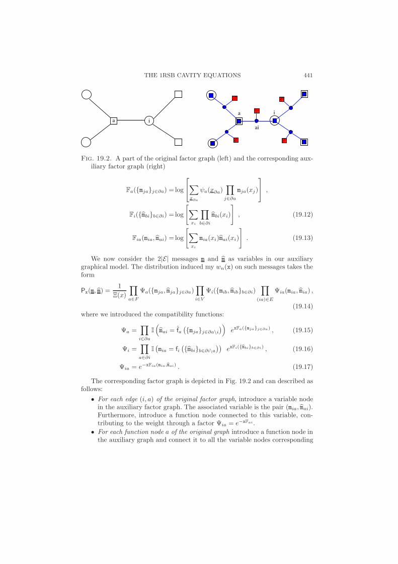
Fig. 19.2. A part of the original factor graph (left) and the corresponding aux-iliary factor graph (right)
Fa(mjaj∈∂a) = log
∑
x∂a
ψa(x∂a)∏
j∈∂a
mja(xj)
,
Fi(mbib∈∂i) = log
[∑
xi
∏
b∈∂i
mbi(xi)
], (19.12)
Fia(mia, mai) = log
[∑
xi
mia(xi)mai(xi)
]. (19.13)
We now consider the 2|E| messages m and m as variables in our auxiliarygraphical model. The distribution induced my wn(x) on such messages takes theform
Px(m, m) =1
Ξ(x)
∏
a∈F
Ψa(mja, mjaj∈∂a)∏
i∈V
Ψi(mib, mibb∈∂i)∏
(ia)∈E
Ψia(mia, mia) ,
(19.14)where we introduced the compatibility functions:
Ψa =∏
i∈∂a
I(mai = fa
(mjaj∈∂a\i
))exFa(mjaj∈∂a) , (19.15)
Ψi =∏
a∈∂i
I(mia = fi
(mbib∈∂i\a
))exFi(bmbib∈∂i) , (19.16)
Ψia = e−xFia(mia,bmai) . (19.17)
The corresponding factor graph is depicted in Fig. 19.2 and can described asfollows:
• For each edge (i, a) of the original factor graph, introduce a variable nodein the auxiliary factor graph. The associated variable is the pair (mia, mai).Furthermore, introduce a function node connected to this variable, con-tributing to the weight through a factor Ψia = e−xFai.
• For each function node a of the original graph introduce a function node inthe auxiliary graph and connect it to all the variable nodes corresponding
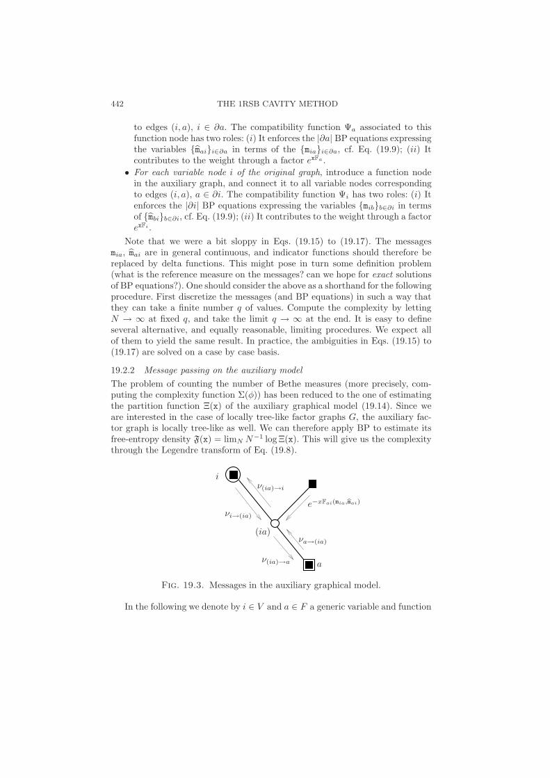
442 THE 1RSB CAVITY METHOD
to edges (i, a), i ∈ ∂a. The compatibility function Ψa associated to thisfunction node has two roles: (i) It enforces the |∂a| BP equations expressingthe variables maii∈∂a in terms of the miai∈∂a, cf. Eq. (19.9); (ii) Itcontributes to the weight through a factor exFa .
• For each variable node i of the original graph, introduce a function nodein the auxiliary graph, and connect it to all variable nodes correspondingto edges (i, a), a ∈ ∂i. The compatibility function Ψi has two roles: (i) Itenforces the |∂i| BP equations expressing the variables mibb∈∂i in termsof mbib∈∂i, cf. Eq. (19.9); (ii) It contributes to the weight through a factorexFi .
Note that we were a bit sloppy in Eqs. (19.15) to (19.17). The messagesmia, mai are in general continuous, and indicator functions should therefore bereplaced by delta functions. This might pose in turn some definition problem(what is the reference measure on the messages? can we hope for exact solutionsof BP equations?). One should consider the above as a shorthand for the followingprocedure. First discretize the messages (and BP equations) in such a way thatthey can take a finite number q of values. Compute the complexity by lettingN → ∞ at fixed q, and take the limit q → ∞ at the end. It is easy to defineseveral alternative, and equally reasonable, limiting procedures. We expect allof them to yield the same result. In practice, the ambiguities in Eqs. (19.15) to(19.17) are solved on a case by case basis.
19.2.2 Message passing on the auxiliary model
The problem of counting the number of Bethe measures (more precisely, com-puting the complexity function Σ(φ)) has been reduced to the one of estimatingthe partition function Ξ(x) of the auxiliary graphical model (19.14). Since weare interested in the case of locally tree-like factor graphs G, the auxiliary fac-tor graph is locally tree-like as well. We can therefore apply BP to estimate itsfree-entropy density F(x) = limN N−1 logΞ(x). This will give us the complexitythrough the Legendre transform of Eq. (19.8).
i
(ia)
aν(ia)→a
ν(ia)→i
νa→(ia)
νi→(ia)
e−xFai(mia,bmai)
Fig. 19.3. Messages in the auxiliary graphical model.
In the following we denote by i ∈ V and a ∈ F a generic variable and function

THE 1RSB CAVITY EQUATIONS 443
node in the graph G, and by (ia) ∈ E an edge in G. By extension, we denotein the same way the corresponding nodes in the auxiliary graph. The messagesappearing in the BP analysis of the auxiliary model can be classified as follows,cf. Fig. 19.3:
→ From the variable node (ia) are issued two messages: ν(ia)→a(mia, mai) andν(ia)→i(mia, mai)
→ From the function node a are issued |∂a| messages to nodes i ∈ ∂a,νa→(ai)(mia, mai)
→ From the function node i are issued |∂i| messages to nodes a ∈ ∂i,νi→(ai)(mia, mai)
→ From the degree-one function node connected to the variable node (ia) is is-sued a message towards this variable. This message is simply e−xFia(mia,bmai).
The BP equations on the variable node (ia) take a simple form:
ν(ia)→a(mia, mai) ∼= νi→(ia)(mia, mai) e−xFia(mia,bmai) ,
ν(ia)→i(mia, mai) ∼= νa→(ia)(mia, mai) e−xFia(mia,bmai) . (19.18)
We can use these equations to eliminate messages νi→(ia), νa→(ia) in favor ofν(ia)→a, ν(ia)→i. In order to emphasize this choice (and to simplify notations) wedefine:
Qia(mia, mai) ≡ ν(ia)→a(mia, mai) , Qai(mia, mai) ≡ ν(ia)→i(mia, mai) .(19.19)
We can now write the remaining BP equations of the auxiliary graphicalmodel in terms of Qia( · , · ), Qai( · , · ). The BP equation associated to the func-tion node corresponding to i ∈ V reads:
Qia(mia, mai) ∼=∑
mib,bmbib∈∂i\a
[∏
c∈∂i
I(mic = fi(mdid∈∂i\c)
)]
expx [Fi (mbib∈∂i) − Fai (mia, mai)]
∏
b∈∂i\a
Qbi(mib, mbi) , (19.20)
and the one associated to the function node corresponding to a ∈ F is:
Q ai(mia, mai) ∼=∑
mja,bmajj∈∂a\i
∏
j∈∂a
I(maj = fa(mkak∈∂a\j)
)
(19.21)
expx[Fa
(mjaj∈∂a
− Fai (mia, mai)
]) ∏
j∈∂a\i
Qja(mja, maj) . (19.22)
Equations (19.20), (19.22) can be further simplified, using the following lemma.

444 THE 1RSB CAVITY METHOD
Lemma 19.3 Assume∑
ximia(xi)mai(xi) > 0. Under the condition mia = fi(mdid∈∂i\a)
(in particular if the indicator functions in Eq. (19.20) evaluate to 1), the dif-ference Fi (mbib∈∂i) − Fai (mia, mai) can be expressed in terms of mbib∈∂i\a.Explicitly, we have
eFi−Fia = zia(mbib∈∂i\a) ≡∑
xi
∏
b∈∂i\a
mbi(xi) . (19.23)
Analogously, under the condition mai = fa(mkak∈∂a\i) (in particular if theindicator functions in Eq. (19.22) evaluate to 1) the difference Fa (mjaj∈∂a)−Fai (mia, mai) depends only on mjaj∈∂a\i. Explicitly:
eFa−Fia = zai(mjaj∈∂a\i) ≡∑
x∂a
ψa(x∂a)∏
j∈∂a\i
mja(xj) . (19.24)
Proof: Let us first consider Eq. (19.23). From the definition (14.28), it followsthat
eFi−Fia =
∑xi
∏b∈∂i mbi(xi)∑
ximia(xi)mai(xi)
. (19.25)
Substituting mia = fi(mcic∈∂i\a) in the denominator, and keeping track of thenormalization constant, we get
∑
xi
mia(xi)mai(xi) =
∑xi
∏b∈∂i mbi(xi)∑
xi
∏b∈∂i\a mai(xi)
, (19.26)
which implies Eq. (19.23).The derivation of Eq. (19.24) is completely analogous and left as an exercise
for the reader. !Notice that the functions zia( · ), zai( · ) appearing in Eqs. (19.23), (19.24) are
in fact the normalization constants hidden by the ∼= notation in Eqs. (19.9).Because of this lemma, we can seek a solution of Eqs. (19.20), (19.22) with
Qia depending only on mia, and Qai depends only on mai. Hereafter we shall focuson this case, and, with an abuse of notation, we shall write:
Qia(mia, mai) = Qia(mia) , Qia(mia, mai) = Qai(mai) . (19.27)
The BP equations for the auxiliary graphical model (19.20), (19.22) then become:
Qia(mia) ∼=∑
bmbi
I (mia = gi(mbi)) [zia(mbi)]x∏
b∈∂i\a
Qbi(mbi) , (19.28)
Qai(mai) ∼=∑
mja
I (mai = fa(mja)) [zai(mja)]x∏
j∈∂a\i
Qja(mja) , (19.29)
where mbi is a shorthand for mbib∈∂i\a and mja a shorthand for mjaj∈∂a\i.The expressions for zia(mbi) and zai(mja) are given in Eqs. (19.23), (19.24).

THE 1RSB CAVITY EQUATIONS 445
Equations (19.28), (19.29) are the 1RSB cavity equations. As we did inthe ordinary BP equations, we can consider them as an update rule for a messagepassing algorithm. This will be further discussed in the next sections. One some-times uses the notation Qi→a( · ), Qa→i( · ), to emphasize the fact that 1RSBmessages are associated to directed edges.
Notice that our derivation was based on the assumption that∑
ximia(xi)mai(xi) >
0. This condition holds if, for instance, the compatibility functions of the originalmodel are bounded away from 0. Under this condition, we have shown that:
Proposition 19.4 If the 1RSB cavity equations (19.28), (19.29) have a solutionQ, Q, this corresponds to a solution to the BP equations of the auxiliary graphicalmodel. Reciprocally, if the BP equations of the auxiliary graphical model admit asolution satisfying the condition (19.27), then the resulting messages must be asolution of the 1RSB cavity equations.
Assumption (19.27) -which is suggestive of a form of “causality”- cannot befurther justified within the present approach, but alternative derivations of the1RSB equations confirm its validity.
19.2.3 Computing the complexity
We now compute the free-entropy of the auxiliary graphical model within the BPapproximation. We expect the result of this procedure to be asymptotically exactfor a wide class of locally tree like graphs, thus yielding the correct free-entropydensity F(x) = limN N−1 logΞ(x).
Assume Qia, Qai to be a solution (or a quasi-solution) of the 1RSB cavityequations (19.28), (19.29). We use the general form (14.27) of Bethe free-entropy,but take into account the degree one factor nodes using the simplified expressionderived in Exercise 14.6. The various contributions to the free-entropy are:
→ Contribution from the function node a (here mia is a shorthand formiai∈∂a):
FRSBa = log
∑
mia
exFa(mia)∏
i∈∂a
Qia(mia)
. (19.30)
→ Contribution from the function node i (mai is a shorthand for maia∈∂i):
FRSBi = log
∑
bmai
exFi(bmai)∏
a∈∂i
Qai(mai)
. (19.31)
→ Contribution from the variable node (ia):
FRSBia = log
∑
mia,bmai
exFia(mia,bmai)Qia(mia)Qai(mai)
. (19.32)

446 THE 1RSB CAVITY METHOD
→ The contributions from the two edges a− (ai) and i− (ai) are both equalto −FRSB
ia
The Bethe free-entropy of the auxiliary graphical model is equal to:
FRSB(Q, Q) =∑
a∈F
FRSBa +
∑
i∈V
FRSBi −
∑
(ia)∈E
FRSBia . (19.33)
19.2.4 Summary
The 1RSB cavity equations (19.28), (19.29) are BP equations for the auxiliarygraphical model defined in (19.14). They relate 2|E| messages Qia(mia), Qai(mai).Each such message is a probability distribution of ordinary BP messages, respec-tively mia(xi) and mai(xi). These elementary messages are in turn probabilitydistributions on variables xi ∈ X .
Given a solution (or an approximate solution) Qia, Qai, one can estimatethe free-entropy density of the auxiliary model as
logΞ(x) = FRSB(Q, Q) + errN . (19.34)
where FRSB(Q, Q) is given by Eq. (19.33). For a large class of locally tree-like models we expect the BP approximation to be asymptotically exact on theauxiliary model. This means that the error term errN is o(N).
For such models, the free-entropy density is given by its 1RSB cavity expres-sion F(x) = fRSB(x) ≡ limN→∞ FRSB(Q, Q)/N . The complexity Σ(φ) is thencomputed through the Legendre transform (19.8).
19.2.5 Random graphical models and density evolution
Let us consider the case where G is a random graphical model as defined inSec. 14.6.1. The factor graph is distributed according to one of the ensemblesGN(K,α) or DN (Λ, P ). Function nodes are taken from a finite list ψ(k)(x1, . . . , xk; J)indexed by a label J with distribution P (k)
bJ. Each factor ψa( · ) is taken equal
to ψ(k)( · · · ; Ja) independently with the same distribution. We also introduceexplicitly a degree-one factor ψi(xi) connected to each variable node i ∈ V . Thisare also drawn independently from a list of possible factors ψ(x; J), indexedby a label J with distribution PJ .
For a random graphical model, the measure µ( · ) becomes random, and sodoes its decomposition in extremal Bethe states, in particular the probabili-ties wn, and the message sets νn
i→a, νna→i. In particular, the 1RSB messages
Qia, Qai become random. It is important to keep in mind the ‘two levels’ ofrandomness. Given an edge (ia), the message νn
i→a is random if the Bethe staten is drawn from the distribution wn. The resulting distribution Qia(m) becomesa random variable when the graphical model is itself random.
The distributions of Qia(m), Qai(m) can then be studied through the density
evolution method of Sec. 14.6.2. Let us assume an i.i.d. initialization Q(0)ia ( · ) d
=

THE 1RSB CAVITY EQUATIONS 447
Q(0)( · ) (respectively Q(0)ai ( · ) d
= Q(0)( · )), and denote by Q(t)ia ( · ), Q(t)
ai ( · ) the1RSB messages along edge (ia) after t parallel updates using the 1RSB equa-tions (19.28), (19.29). If (ia) is a uniformly random edge then, as N → ∞,
Q(t)ia ( · ) converges in distribution29 to Q(t)( · ) (respectively Q(t)
ia ( · ) converges in
distribution to Q(t)( · )). The distributions Q(t)( · ) and Q(t)( · ) are themselvesrandom variables that satisfy the equations:
Q(t+1)(m)d∼=∑
bmb
I (m = f(mb; J)) z(mb; J)xl−1∏
b=1
Q(t)b (mb) , (19.35)
Q(t)(m)d∼=∑
mj
I(m = f(mj; J)
)z(mj; J)x
k−1∏
j=1
Q(t)j (mj) , (19.36)
where k and l are distributed according to the edge perspective degree profiles
ρk and λl, theQ(t)
b
are k − 1 independent copies of Q(t)( · ), and
Q(t)
j
are
l − 1 independent copies of Q(t)( · ). The functions z and z are given by:
z(mb; J) =∑
x
ψ(x, J)l−1∏
b=1
mb(x)
z(mj; J) =∑
x1,··· ,xk
ψ(k)(x1, · · · , xk; J)k−1∏
j=1
mj(xj) (19.37)
Within the 1RSB cavity method, the actual distribution of Qi→a is assumedto coincide with one of the fixed points of the above density evolution equations.As for the RS case, one hopes that, on large enough instances, the messagepassing algorithm will converge to messages distributed according to this fixedpoint equation (meaning that there is no problem in exchanging the limits t →∞and N →∞). This can be checked numerically.
For random graphical models, the 1RSB free-entropy density converges to afinite limit fRSB(x). This can be expressed in terms of the distributions of Q,Q. by taking expectation of Eqs. (19.30) to (19.32), and assuming that 1RSBmessages incoming at the same node are i.i.d.. As in (14.77) the result takes theform:
fRSB = fRSBv + nf f
RSBf − nef
RSBe . (19.38)
Here nf is the average number of function nodes per variable (equal to Λ′(1)/P ′(1)for a graphical model in the DN (Λ, P ) ensemble, and to α for a graphical modelin the GN(K,α) ensemble) and ne is the number of edges per variable (equal to
29We shall not discuss the measure-theoretic subtleties related to this statement. Let us justmention that weak topology is understood on the space of messages Q(t).
448 THE 1RSB CAVITY METHOD
Λ′(1) and to Kα in these two ensembles). The contribution from variable nodesfRSBv , function nodes fRSB
f , and edges fRSBe are:
fRSBv = El,J, bQ log
∑
bm1,...,bml
Q1(m1) . . . Ql(ml)
[∑
x∈Xm1(x) . . . ml(x)ψ(x; J)
]x
,
fRSBf = Ek, bJ,Q log
∑
m1,...,mk
Q1(m1) . . . Qk(mk)
∑
x1,...,xk∈Xm1(x1) . . . mk(xk)ψ(k)(x1, . . . , xk; J)
x
,
fRSBe = E bQ,Q log
∑
bm,m
Q(m)Q(m)
[∑
x∈Xm(x)m(x)
]x
. (19.39)
19.2.6 Numerical implementation
Needless to say, it is extremely challenging to find a fixed point of the density evo-lution equations (19.35), (19.36), and thus determine the distributions of Q, Q.A simple numerical approach consists in generalizing the population dynamicsalgorithm described in the context of the RS cavity method, cf. Sec. 14.6.3.
There are two important issues related to such a generalization:
(i) We seek the distribution of Q( · ) (and Q( · )), which is itself a distributionof messages. If we approximate Q( · ) by a sample (a ‘population’), we willthus need two level of populations. In other words we will seek a popula-tion ms
r with NM items. For each r ∈ 1, . . . , N, the set of messagesms
r, s ∈ 1, . . . , M represents a distribution Qr( · ) (ideally, it would bean i.i.d. sample from this distribution). At the next level, the populationQr( · ) , r ∈ 1, · · · , N represents the distribution of Q( · ) (ideally, ani.i.d. sample).
Analogously, for function-to-variable messages, we will use a populationms
r, with r ∈ 1, . . . , N and s ∈ 1, . . . , M.
(ii) The re-weighting factors z(mb; J)x and z(mj; J)x appearing in Eqs. (19.35)and (19.36) do not have any analog in the RS context. How can one takesuch factors into account when Q( · ), Q( · ) are represented as populations?One possibility is to generate an intermediate weighted population, andthan sample from it with a probability proportional to the weight.
This procedure is summarized in the following pseudocode.

THE 1RSB CAVITY EQUATIONS 449
1RSB Population dynamics (Model ensemble, Sizes N, M , Iterations T )1: Initialize ms
r;2: for t = 1, . . . , T :3: for r = 1, . . . , N :4: Draw an integer k with distribution ρ;5: Draw i(1), . . . , i(k − 1) uniformly in 1, . . . , N;6: Draw J with distribution P (k)
bJ;
7: for s = 1, . . . , M :8: Draw s(1), . . . , s(k− 1) uniformly in 1, . . . , M;9: Compute ms
temp = f(ms(1)i(1) , · · · , ms(k−1)
i(k−1) ; J)
10: Compute W s = z(ms(1)i(1) , · · · , ms(k−1)
i(k−1) ; J)x
11: end;12: Generate the new population
msrs∈[M ] = Reweight(ms
temp, Wss∈[M ])
13: end;14: for r = 1, . . . , N :15: Draw an integer l with distribution λ;16: Draw i(1), . . . , i(l − 1) uniformly in 1, . . . , N;17: Draw J with distribution P ;18: for s = 1, . . . , M :19: Draw s(1), . . . , s(l− 1) uniformly in 1, . . . , M;20: Compute ms
temp = f(ms(1)i(1) , · · · , ms(k−1)
i(l−1) ; J)
21: Compute W s = z(ms(1)i(1) , · · · , ms(l−1)
i(l−1) ; J)x
22: end;23: Generate the new population
msrs∈[M ] = Reweight(ms
temp, Wss∈[M ])
24: end;25: return ms
r and msr.
The re-weighting procedure is given by:
Reweight (Population of messages/weights (mstemp, W
s)s∈[M ])
1: for s = 1, . . . , M , set ps ≡ W s/∑
s′ W s′;
2: for s = 1, . . . , M :3: Draw i ∈ 1, . . . , M with distribution ps;4: Set ms
new = mitemp;
5: end;6: return ms
news∈[M ].
In the large N, M limit, the populations generated by this algorithm shouldconverge to i.i.d. samples distributed as Q(T )( · ), Q(T )( · ), cf. Eq. (19.35), (19.36).

450 THE 1RSB CAVITY METHOD
By letting T grow they should represent accurately the fixed points of densityevolution, although the caveats expressed in the RS case should be repeated here.
Among the other quantities, the populations generated by this algorithmallow to estimate the 1RSB free-entropy density (19.38). Suppose we have gen-erated a population of messages ms
r( · ), whereby each message is a probabilitydistribution on X . The corresponding estimate of fRSB
v is:
fRSBv = El,J
1
N l
N∑
r(1)...r(l)=1
log
1
M l
M∑
s(1),...,s(l)=1
[∑
x∈Xm
s(1)r(1)(x) · · · ms(l)
r(l)(x) ψ(x; J)
]x
.
Similar expressions are easily written for fRSBf and fRSB
e . Their (approximate)evaluation can be accelerated considerably by summing over a random subsetof the l-uples r(1), . . . , r(l) and s(1), . . . , s(l). Further, as in the RS case, it isbeneficial to average over iterations (equivalently, over T ) in order to reducestatistical errors at small computational cost.
19.3 A first application: XORSAT
Let us apply the 1RSB cavity method to XORSAT. This approach was alreadyintroduced in Sec. 18.6, but we want to show how it follows as a special case ofthe formalism developed in the previous sections. Our objective is to exemplifythe general ideas on a well understood problem, and to build basic intuition thatwill be useful in more complicated applications.
As in Ch. 18 we consider the distribution over x = (x1, . . . , xN ) ∈ 0, 1N
specified by
µ(x) =1
Z
M∏
a=1
I(xi1(a) ⊕ · · ·⊕ xik(a) = ba
). (19.40)
As usual⊕ denotes sum modulo 2 and, for each a ∈ 1, · · · , M, ∂a = i1(a), . . . , iK(a)is a subset of 1, ·, N, and ba ∈ 0, 1. Random K-XORSAT formulae are gen-erated by choosing both the index set i1(a), . . . , iK(a) and the right hand sideba uniformly at random.
19.3.1 BP equations
The BP equations read:
mia(xi) =1
zia
∏
b∈∂i\a
mbi(xi) , (19.41)
mai(xi) =1
zai
∑
x∂a\i
I(xi1(a) ⊕ · · ·⊕ xiK(a) = ba
) ∏
j∈∂a\i
mja(xj) . (19.42)
As in Sec. 18.6, we shall assume that messages can take only three values, whichwe denote by the shorthands: mia = 0 if (mia(0) = 1, mia(1) = 0); mia = 1 if(mia(0) = 0, mia(1) = 1); mia = ∗ if (mia(0) = mia(1) = 1/2).

A FIRST APPLICATION: XORSAT 451
Consider the first BP equation (19.41), and denote by n0, n1, n∗ the numberof messages of type 0, 1, ∗ in the set of incoming messages mbi, b ∈ ∂i\a. ThenEq. (19.41) can be rewritten as:
mia =
0 if n0 > 0, n1 = 0,1 if n0 = 0, n1 > 0,∗ if n0 = 0, n1 = 0,? if n0 > 0, n1 > 0,
zia =
2−n∗ if n0 > 0, n1 = 0,2−n∗ if n0 = 0, n1 > 0,21−n∗ if n0 = 0, n1 = 0,0 if n0 > 0, n1 > 0.
(19.43)
The computation of the normalization constant zia will be useful in the 1RSBanalysis. Notice that, if n0 > 0 and n1 > 0, a contradiction arises at node iand therefore mia is not defined. However we will see that, because in this casezia = 0, this situation does not create any problem within 1RSB.
In the second BP equation (19.42) denote by n0 (respectively, n1, n∗) thenumber of messages of type 0 (resp. 1, ∗) among mja, j ∈ ∂a\i. Then we get
mai =
0 if n∗ = 0, and n1 has the same parity as ba,1 if n∗ = 0, and n1 has not the same parity as ba,∗ if n∗ > 0.
(19.44)
In all three cases zai = 1.In Sec. 18.6 we studied the equations (19.41), (19.42) above and deduced
that, for typical random instances with α = M/N < αd(K), they have a uniquesolution, with mia = mai = ∗ on each edge.
Exercise 19.2 Evaluate the Bethe free-entropy on this solution, and showthat it yields the free-entropy density fRS = (1 − α) log 2.
19.3.2 The 1RSB cavity equations
We now assume that the BP equations (19.43), (19.44) have many solutions, andapply the 1RSB cavity method to study their statistics.
The 1RSB messages Qia, Qai are distributions over 0, 1, ∗. A little effortshows that Eq. (19.28) yields
Qia(0) =1
Zia
∏
b∈∂i\a
(Qbi(0) + 2−xQbi(∗)
)−
∏
b∈∂i\a
(2−xQbi(∗)
)
,(19.45)
Qia(1) =1
Zia
∏
b∈∂i\a
(Qbi(1) + 2−xQbi(∗)
)−
∏
b∈∂i\a
(2−xQbi(∗)
)
,(19.46)
Qia(∗) =1
Zia2x
∏
b∈∂i\a
2−xQbi(∗) . (19.47)
For instance, Eq. (19.45) follows from the first line of Eq. (19.43): mia = 0 ifall the incoming messages are mbi ∈ ∗, 0 (first term), unless they are all equal

452 THE 1RSB CAVITY METHOD
to ∗ (subtracted term). The re-weighting zxia = 2−xn∗ decomposes into factorsassociated to the incoming ∗ messages.
The second group of 1RSB equations, Eq. (19.29), takes the form:
Qai(0) =1
2
∏
j∈∂a\i
(Qja(0) + Qja(1)) + s(ba)∏
j∈∂a\i
(Qja(0) −Qja(1))
,
(19.48)
Qai(1) =1
2
∏
j∈∂a\i
(Qja(0) + Qja(1)) − s(ba)∏
j∈∂a\i
(Qja(0) −Qja(1))
,
(19.49)
Qai(∗) = 1 −∏
j∈∂a\i
(Qja(0) + Qja(1)) , (19.50)
where s(ba) = +1 if ba = 0, and s(ba) = −1 otherwise.Notice that, if one takes x = 0, the two sets of equations coincide with those
obtained in Sec. 18.6, see Eq. (18.35) (the homogeneous linear system, ba = 0, wasconsidered there). As in that section, we look for solutions such that the messagesQia( · ) (respectively Qai( · )) take two possible values: either Qia(0) = Qia(1) =1/2, or Qia(∗) = 1. This assumption is consistent with the 1RSB cavity equations(19.45) and (19.50). Under this assumption, the x dependency drops from theseequations and we recover the analysis in Sec. 18.6. In particular, we can repeatthe density evolution analysis discussed there. If we denote by Q∗ the probabilitythat a randomly chosen edge carries the 1RSB message Qia(0) = Qia(1) = 1/2,then the fixed point equation of density evolution reads:
Q∗ = 1 − exp−kαQk−1∗ . (19.51)
For α < αd(K) this equation admits the only solution Q∗ = 0, implying Qia(∗) =1 with high probability. This indicates (once more) that the only solution of theBP equations in this regime is mia = ∗ for all (i, a) ∈ E.
For α > αd a couple of non-trivial solutions (with Q∗ > 0) appear, indicatingthe existence of a large number of BP fixed points (and hence, Bethe measures).Stability under density evolution suggest to select the largest one. It will also beuseful in the following to introduce the probability
Q∗ = Qk−1∗ (19.52)
that a uniformly random edge carries a message Qai(0) = Qai(1) = 1/2.
19.3.3 Complexity
We can now compute the Bethe free-entropy (19.33) of the auxiliary graphicalmodel. The complexity will be computed through the Legendre transform of the1RSB free-entropy, see Eq. (19.8).
A FIRST APPLICATION: XORSAT 453
Let us start by computing the contribution FRSBa defined in Eq. (19.30). Con-
sider the weight
eFa(mia) =∑
x∂a
I(xi1(a) ⊕ · · ·⊕ xiK(a) = ba)∏
i∈∂a
mia(xi) . (19.53)
Let n0 (respectively, n1, n∗) denote the number of variable nodes i ∈ ∂a suchthat mia = 0 (resp. 1, ∗) for i ∈ ∂a. Then we get
eFa(mia) =
1/2 if n∗ > 0,1 if n∗ = 0 and n1 has the same parity as ba,0 if n∗ = 0 and n1 has not the same parity as ba,
(19.54)
Taking the expectation of exFa(mia) with respect to mia distributed indepen-dently according to Qia( · ), and assuming Qia(0) = Qia(1) (which is the case inour solution), we get
FRSBa = log
1
2
∏
i∈∂a
(1 −Qia(∗)) +1
2x
[1 −
∏
i∈∂a
(1 −Qia(∗))]
. (19.55)
The first term corresponds to the case n∗ = 0 (the factor 1/2 being the proba-bility that the parity of n1 is ba), and the second to n∗ > 0. Within our solutioneither Qia(∗) = 0 or Qia(∗) = 1. Therefore only one of the above terms survives:either Qia(∗) = 0 for all i ∈ ∂a, yielding FRSB
a = − log 2, or Qia(∗) = 1 for somei ∈ ∂a, implying FRSB
a = −x log 2.Until now we considered a generic K-XORSAT instance. For random in-
stances, we can take the expectation with respect to Qia(∗) independently dis-tributed as in the density evolution fixed point. The first case, namely Qia(∗) = 0for all i ∈ ∂a (and thus FRSB
a = − log 2), occurs with probability Qk∗. The second,
i.e. Qia(∗) = 1 for some i ∈ ∂a (and FRSBa = −x log 2), occurs with probability
1 −Qk∗ . Altogether we obtain:
EFRSBa = −
[Qk
∗ + x(1 −Qk∗)]
log 2 + oN (1) . (19.56)
Assuming the messages Qia( · ) to be short-range correlated,∑
a∈F FRSBa will
concentrate around its expectation. We then have, with high probability,
1
N
∑
a∈F
FRSBa = −α
[Qk
∗ + x(1 −Qk∗)]
log 2 + oN (1) . (19.57)
The contributions from variable node and edge terms can be computed alongsimilar lines. We will just sketch these computations, and invite the reader towork out the details.
Consider the contribution FRSBi , i ∈ V , defined in (19.31). Assume that
Qai(∗) = 1 (respectively, Qai(0) = Qai(1) = 1/2) for n∗ (resp. n0) of the neigh-boring function nodes a ∈ ∂i. Then FRSB
i = −(n∗x + n0 − 1) log 2 if n0 ≥ 1, and

454 THE 1RSB CAVITY METHOD
FRSBi = −(n∗ − 1)x log 2 otherwise. Averaging these expressions over n0 (a Pois-
son distributed random variable with mean kαQ∗) and n∗ (Poisson with meankα(1 − Q∗)) we obtain:
1
N
∑
i∈V
FRSBi = −
[kαQ∗ − 1 + e−kα bQ∗
]+[kα(1 − Q∗) − e−kα bQ∗
]x
log 2+oN(1) .
(19.58)Let us finally consider the edge contribution FRSB
(ia) defined in (19.32). If
Qia(0) = Qia(1) = 1/2 and Qai(0) = Qai(1) = 1/2, then either eFai = 1 oreFia = 0, each with probability 1/2. As a consequence FRSB
(ia) = − log 2. If ei-
ther Qia(∗) = 1 or Qai(∗) = 1 (or both), eFRSBia = 1/2 with probability 1, and
therefore FRSB(ia) = −x log 2. Altogether we obtain, with high probability
1
N
∑
(ia)∈E
FRSB(ia) = −kα
Q∗Q∗ + (1 −Q∗Q∗)x
log 2 + oN (1). (19.59)
The free-entropy (19.33) of the auxiliary graphical model is obtained bycollecting the various terms. We obtain FRSB(x) = N fRSB(x) + o(N) wherefRSB(x) = [Σtot + xφtyp] log 2 and
Σtot = kαQ∗Q∗ − kαQ∗ − αQk∗ + 1 − e−kα bQ∗ , (19.60)
φtyp = −kαQ∗Q∗ + kαQ∗ + αQk∗ − α + e−kα bQ∗ . (19.61)
Here Q∗ is the largest solution of Eq. (19.51) and Q∗ = Qk−1∗ , a condition that
has a pleasing interpretation as shown in the exercise below.
Exercise 19.3 Consider the function Σtot(Q∗, Q∗) defined in Eq. (19.60).Show that the stationary points of this function coincide with the solutionsof Eq. (19.51) and Q∗ = Qk−1
∗ .
Because of the linear dependence on x, the Legendre transform (19.8) isstraightforward
Σ(φ) =
Σtot if φ = φtyp,−∞ otherwise.
(19.62)
This means that there are 2NΣtot Bethe measures which all have the same entropyNφtyp log 2. Furthermore, Σtot + φtyp = 1−α, confirming that the total entropyis (1 − α) log 2. This identity can be also written in the form
1
2N(1−α)=
1
2NΣtot× 1
2Nφtyp, (19.63)
which is nothing but the decomposition (19.6) in extremal Bethe measures. In-deed, if x is a solution of the linear system, µ(x) = 1/2N(1−α), wn ≈ 1/2NΣtot ,

THE SPECIAL VALUE X = 1 455
and (assuming the µn to have disjoint supports) µn(x) ≈ 1/2Nφtyp for the staten which contains x.
Note that the value of Σ that we find here coincides with the result thatwe obtained in Sec. 18.5 for the logarithm of the number of clusters in randomXORSAT formulae. This provides an independent check of our assumptions, andin particular it shows that the number of clusters is, to leading order, the same asthe number of Bethe measures. In particular, the SAT-UNSAT transition occursat the value of α where the complexity Σtot vanishes. At this value each clusterstill contains a large number, 2N(1−αs), of configurations.
Exercise 19.4 Repeat this 1RSB cavity analysis for a linear Boolean systemdescribed by a factor graph from the ensemble DN (Λ, P ) (This means a randomsystem of linear equations, whereby the fraction of equations involving k vari-ables is Pk, and the fraction of variables which appear in exactly - equationsis Λ%):
(a) Show that Q∗ and Q∗ satisfy:
Q∗ = ρ(Q∗) ; Q∗ = 1 − λ(1 − Q∗) , (19.64)
where λ and ρ are the edge perspective degree profiles.(b) Show that the complexity is given by
Σtot = 1 − Λ′(1)
P ′(1)P (Q∗)− Λ(1 − Q∗) − Λ′(1)(1 −Q∗)Q∗ (19.65)
and the internal entropy of the clusters is φtyp = 1− Λ′(1)/P ′(1)−Σtot.(c) In the case where all variables have degree strictly larger than 1 (so that
λ(0) = 0), argue that the relevant solution is Q∗ = Q∗ = 1, Σtot =1 − Λ′(1)/P ′(1), φtyp = 0. What is the interpretation of this result interms of the core structure discussed in Sec. 18.3?
19.4 The special value x = 1
Let us return to the general formalism. The x = 1 case plays a special role,in that the weights wn(x) of various Bethe measures in the auxiliary model,coincide with the ones appearing in the decomposition (19.6). This fact manifestsitself in some remarkable properties of the 1RSB formalism.
19.4.1 Back to BP
Consider the general 1RSB cavity equations (19.28), (19.29). Using the explicitform of the re-weighting factors eFi−Fia and eFa−Fia provided in Eqs. (19.23),(19.24), they can be written, for x = 1, as:

456 THE 1RSB CAVITY METHOD
Qia(mia) ∼=∑
xi
∑
bmbi
I (mia = gi(mbi))∏
b∈∂i\a
Qbi(mbi) mbi(xi) , (19.66)
Qai(mai) ∼=∑
x∂a
ψa(x∂a)∑
mja
I (mai = fa(mja))∏
j∈∂a\i
Qja(mja) mja(xj) .(19.67)
Let us introduce the messages obtained by taking the averages of the 1RSB onesQia, Qai:
νavi→a(xi) ≡
∑
mia
Qia(mia) mia(xi) , νava→i(xi) ≡
∑
bmai
Qai(mai) mai(xi) .
The interpretation of these quantities is straightforward. Given an extremalBethe measure sampled according to the distribution wn, let νn
i→a( · ) (respec-tively νn
a→i( · )) be the corresponding message along the directed edge i → a(resp. a → i). Its expectation, with respect to the random choice of the measure,is νav
i→a( · ) (respectively νava→i( · )).
Using the expressions (19.9), one finds that Eqs. (19.66), (19.67) imply
νavi→a(xi) ∼=
∏
b∈∂i\a
νavb→i(xi) , (19.68)
νava→i(xi) ∼=
∑
xjj∈∂a\i
ψa(x∂a)∏
j∈∂a\i
νavj→a(xj) , (19.69)
which are nothing but the ordinary BP equations. This suggests that, even if µ( · )decomposes into an exponential number of extremal Bethe measures µn( · ), it isitself a (non-extremal) Bethe measure. In particular, there exists a quasi-solutionof BP equations associated with it, that allows to compute its marginals.
The reader might be disappointed by these remarks. Why insisting on the1RSB cavity approach if, when the ‘correct’ weights are used, one recovers themuch simpler BP equations? There are at least two answers:
1. The 1RSB approach provides a much more refined picture: decompositionin extremal Bethe states, long range correlations, complexity. This is usefuland interesting per se.
2. In the cases of a static (s1RSB) phase, it turns out that the region x = 1corresponds to an ‘unphysical’ solution of the 1RSB cavity equations, andthat (asymptotically) correct marginals are instead obtained by lettingx = x∗, for some x∗ ∈ [0, 1). In such cases it is mandatory to resort to thefull 1RSB formalism (see Sec. 19.6 below).
19.4.2 A simpler recursion
As we stressed above, controlling (either numerically or analytically) the 1RSBdistributional recursions (19.35), (19.36) is a difficult task. In the case x = 1, theysimplify considerably and lend themselves to a much more accurate numericalstudy. This remark can be very useful in practice.

THE SPECIAL VALUE X = 1 457
As in Sec. 19.2.5, we consider a random graphical model. We shall also assumea ‘local uniformity condition.’ More precisely, the original model µ( · ) is a Bethemeasure for the message set νav
i→a(xi) = 1/q and νava→i(xi) = 1/q, where q = |X | is
the size of the alphabet. While such a local uniformity condition is not necessary,it considerably simplify the derivation below. The reader can find a more generaltreatment in the literature.
Consider Eqs. (19.35) and (19.36) at x = 1. The normalization constants canbe easily computed using the uniformity condition. We can then average overthe structure of the graph, and the function node distribution: let us denote byQav and Qav the averaged distributions. They satisfy the following equations:
Q(t+1)av (m) = E
ql−2∑
bmb
I (m = f(mb; J)) z(mb)l−1∏
b=1
Q(t)av (mb)
, (19.70)
Q(t)av (m) = E
qk−2
ψk
∑
mj
I(m = f(mj; J)
)z(mj; J)
k−1∏
j=1
Q(t)av (mj)
, (19.71)
where expectations are taken over l, k, J, J , distributed according to the randomgraphical model. Here ψk =
∑x1,...,xk−1
ψ(x1, . . . , xk−1, x; J) can be shown to be
independent of x (this is necessary for the uniformity condition to hold).Equations (19.70) and (19.71) are considerably simpler that the original dis-
tributional equations (19.35), (19.36) in that Q(t)av ( · ), Q(t)
av ( · ) are non-random.On the other hand, they still involve a reweighting factor that is difficult to han-dle. It turns out that this reweighting can be eliminated by introducing a newcouple of distributions for each x ∈ X :
R(t)x (m) ≡ q m(x) Q(t)
av (m) , R(t)x (m) = q m(x) Q(t)
av (m) . (19.72)
One can show that Eqs. (19.70), (19.71) imply the following recursions for R(t)x ,
R(t)x ,
R(t+1)x (m) = E
∑
bmb
I (m = g(mb; J))l−1∏
b=1
R(t)x (mb)
, (19.73)
R(t)x (m) = E
∑
xj
π(xj|x; J)∑
mj
I(m = f(mj; J)
) k−1∏
j=1
R(t)xj
(mj)
.(19.74)
Here E denotes expectation with respect to l, J, k, J and, for any x, J , the dis-tribution π(xj|x; J) is defined by
π(x1, . . . , xk−1|x; J) =ψ(x1, . . . , xk−1, x; J)
∑y1,...,yk−1
ψ(y1, . . . , yk−1, x; J). (19.75)

458 THE 1RSB CAVITY METHOD
Exercise 19.5 Prove formulas (19.73) and (19.74). It might be useful to recallthe following explicit expressions for the reweighting factors z and z:
z(mb) m(x) =l−1∏
b=1
mb(x) , (19.76)
z(mj; J) m(x) =∑
xi,x
ψ(x1, . . . , xk−1, x; J)k−1∏
j=1
mj(xj) . (19.77)
The equations (19.73), (19.74) have a simple operational description. Let Jand k be drawn according to their distribution, and, given x, generate x1, . . . , xk−1
according to the kernel π(x1, . . . , xk|x; J). Then draw independent messages
m1, . . . , mk−1 with distribution (respectively) R(t)x1 , . . . , R(t)
xk−1 . According to Eq. (19.74),
m = f(mj; J) has then distribution R(t)x . For Eq. (19.73), draw J and l accord-
ing to their distribution. Given x, draw l − 1 i.i.d. messages m1, . . . , ml−1 with
distribution R(t)x . Them m = g(mb; J) has distribution R(t+1)
x .We will see in Ch. 22 that this procedure does indeed coincide with the one
for computing ‘point-to-set correlations’ with respect to the measure µ( · ).To summarize, for x = 1 we have succeeded in simplifying the 1RSB density
evolution equations in two directions: (i) The resulting equations do not involve‘distributions of distributions;’ (ii) We got rid of the reweighting factor. A thirdcrucial simplification is the following:
Theorem 19.5 The 1RSB equations have a non trivial solution (meaning asolution different from the RS one) if and only if Eqs. (19.73), (19.74), when
initialized with R(0)x being a singleton distribution on m(y) = I(y = x), converge
as t →∞, to a non-trivial distribution.
This theorem resolves (in the case x = 1) the ambiguity on the initial conditionof the 1RSB iteration. In other words, if the 1RSB equations admit a non-trivialsolution, it can be reached if we iterate the equations starting from the initialcondition mentioned in the theorem. We refer the reader to the literature for theproof.
Exercise 19.6 Show that the free-entropy of the auxiliary model FRSB(x),evaluated at x = 1, coincides with the RS Bethe free-entropy.
Further, its derivative with respect to x at x = 1 can be expressed in terms of
the fixed point distributions R(∞)x and R(∞)
x . In particular the complexity andinternal free-entropy can be computed from the fixed points of the simplifiedequations (19.73), (19.74).
The conclusion of this section is that 1RSB calculations at x = 1 are nottechnically harder that RS ones. In view of the special role played by the value

SURVEY PROPAGATION 459
x = 1 this observation can be exploited in a number of contexts.
19.5 Survey propagation
The 1RSB cavity method can be applied to other message passing algorithmswhenever these have many fixed points. A particularly important case is the min-sum algorithm of Sec. 14.3. This approach (both in its RS and 1RSB versions)is sometimes referred to as the energetic cavity method because, in physicsterms, the min-sum algorithm aims at computing the ground state configurationand its energy. We will call the corresponding 1RSB message passing algorithmSP(y) (survey propagation at finite y).
19.5.1 The SP(y) equations
The formalism follows closely the one used with BP solutions. To emphasize thesimilarities, let us adopt the same notation for the min-sum messages as for theBP ones. We define
mja(xj) ≡ Ei→a(xi) , mai(xi) ≡ Ea→i(xi) , (19.78)
and write the min-sum equations (14.40), (14.41) as:
mia = fei(mbib∈∂i\a
), mai = fea
(mjaj∈∂a\i
). (19.79)
The functions fei , fea are defined by Eqs. (14.40), (14.41), that we reproduce here:
mia(xi) =∑
b∈∂i\a
mbi(xi)− uia , (19.80)
mai(xi) = minx∂a\i
Ea(x∂a) +∑
j∈∂a\i
mja(xj)
− uai , (19.81)
where uia, uai are normalization constants (independent of xi) which ensure thatminxi mai(xi) = 0 and minxi mia(xi) = 0.
To any set of messages mia, mai, we associate the Bethe energy
Fe(m, m) =∑
a∈F
Fea(miai∈∂a) +
∑
i∈V
Fei (maia∈∂i) −
∑
(ia)∈E
Feia(mia, mai) , (19.82)
where the various terms are (see Eq. (14.45)):
Fea = min
x∂a
[Ea(x∂a) +
∑
j∈∂a
mia(xi)], Fe
i = minxi
[ ∑
a∈∂i
mai(xi)],
Feia = min
xi
[mia(xi) + mai(xi)
]. (19.83)
Having set up the message passing algorithm and the associated energy func-tional, we can repeat the program developed in the previous Sections. In partic-ular, in analogy with Assumption 1, we have the following

460 THE 1RSB CAVITY METHOD
Assumption 4 There exist exponentially many quasi-solutions mn of min-sum equations. The number of such solutions with Bethe energy Fe(mn) ≈ Nεis (to leading exponential order) expNΣe(ε), where Σe(ε) is the energeticcomplexity function.
In order to estimate Σe(ε), we introduce an auxiliary graphical model, whosevariables are the min-sum messages mia, mai. These are forced to satisfy (withinsome accuracy) the min-sum equations (19.80), (19.81). Each solution is given aweight e−yF
e(m,bm), with y ∈ R. The corresponding distribution is:
Py(m, m) =1
Ξ(y)
∏
a∈F
Ψa(mja, mjaj∈∂a)∏
i∈V
Ψi(mib, mibb∈∂i)∏
(ia)∈E
Ψia(mia, mia) ,
(19.84)where:
Ψa =∏
i∈∂a
I(mai = fea
(mjaj∈∂a\i
))e−yF
ea(mjaj∈∂a) , (19.85)
Ψi =∏
a∈∂i
I(mia = fei
(mbib∈∂i\a
))e−yF
ei(bmbib∈∂i) , (19.86)
Ψia = eyFeia(mia,bmai) . (19.87)
Since the auxiliary graphical model is again locally tree-like, we can hopeto derive asymptotically exact results through belief propagation. Messages ofthe auxiliary problem, to be denoted as Qia( · ), Qai( · ), are distributions overthe min-sum messages. The SP(y) equations are obtained by further making theindependence assumption (19.27).
The reader has certainly noticed that the whole procedure is extremely closeto our study in Sec. 19.2.2. We can apply our previous analysis verbatim toderive the SP(y) update equations. The only step that requires some care is theformulation of the proper analog of Lemma 19.3. This becomes:
Lemma 19.6 Assume that mia(xi) + mai(xi) < ∞ for at least one value ofxi ∈ X . If mia = fei (mbib∈∂i\a), then
Fei − Fe
ia = uia(mbib∈∂i\a) ≡ minxi
∑
b∈∂i\a
mbi(xi)
. (19.88)
Analogously, if mai = f ea(mjaj∈∂a\i), then
Fea − Fe
ia = uai(mjaj∈∂a\i) ≡ minx∂a
Ea(x∂a) +
∑
k∈∂a\i
mka(xk)
. (19.89)
Using this lemma, the same derivation as in Sec. 19.2.2 leads to
Proposition 19.7 The SP(y) equations are (with the shorthands mbi for mbib∈∂i\a
and mja for mjaj∈∂a\i):

SURVEY PROPAGATION 461
Qia(mia) ∼=∑
bmbi
I (mia = gei (mbi)) e−yuia(bmbi)
∏
b∈∂i\a
Qbi(mbi) , (19.90)
Qai(mai) ∼=∑
mja
I (mai = f ea(mja)) e−yuai(mja)
∏
j∈∂a\i
Qja(mja) . (19.91)
In the following we shall reserve the name survey propagation (SP) for they = ∞ case of these equations.
19.5.2 Energetic complexity
The Bethe free-entropy for the auxiliary graphical model is given by
FRSB,e(Q, Q) =∑
a∈F
FRSB,ea +
∑
i∈V
FRSB,ei −
∑
(ia)∈E
FRSB,eia , (19.92)
and allows to count the number of min-sum fixed points. The various termsare formally identical to the ones in Eqs. (19.30), (19.31) and (19.32), providedF·( · ) is replaced everywhere by −Fe
· ( · ) and x by y. We reproduce them here forconvenience:
FRSB,ea = log
∑
mia
e−yFea(mia)
∏
i∈∂a
Qia(mia)
, (19.93)
FRSB,ei = log
∑
bmai
e−yFei(bmai)
∏
a∈∂i
Qai(mai)
, (19.94)
FRSB,eia = log
∑
mia,bmai
e−yFeia(mia,bmai)Qia(mia)Qai(mai)
. (19.95)
Assuming that the Bethe free-entropy gives the correct free-entropy of theauxiliary model, the energetic complexity function Σe(ε) can be computed fromFRSB,e(y) through the Legendre transform: in the large N limit we expect FRSB,e(Q, Q) =NFe(y) + o(N) where
Fe(Q, Q) = Σe(ε)− yε ,∂Σe
∂ε= y . (19.96)
Finally, the 1RSB population dynamics algorithm can be used to sample-approximately- the SP(y)messages in random graphical models.
19.5.3 Constraint satisfaction and binary variables
In Sec. 14.3.3 we noticed that the min-sum messages simplify significantly whenone deals with constraint satisfaction problems. In such problems, the energyfunction takes the form E(x) =
∑a Ea(x∂a), where Ea(x∂a) = 0 if constraint
a is satisfied by the assignment x, and Ea(x∂a) = 1 otherwise. As discussed in

462 THE 1RSB CAVITY METHOD
Sec. 14.3.3 the min-sum equations then admit solutions with mai(xi) ∈ 0, 1.Furthermore, one does not need to keep track of the variable-to-function nodemessages mia(xi), but only of their ‘projection’ on 0, 1.
In other words, in constraint satisfaction problems the min-sum messages take2|X |−1 possible values (the all-1 message cannot appear). As a consequence, theSP(y)messages Qai( · ) and Qia( · ) simplify considerably: they are points in the(2|X | − 1)-dimensional simplex.
If the min-sum messages are interpreted in terms of warnings, as we didin Sec. 14.3.3, then SP(y)messages keep track of the warnings’ statistics (overpure states). One can use this interpretation to derive directly the SP(y) updateequations without going through the whole 1RSB formalism. Let us illustratethis approach on the important case of binary variables |X | = 2.
The min-sum messages m and m (once projected) can take three values:(m(0), m(1)) ∈ (0, 1), (1, 0), (0, 0). We shall denote them respectively as 0 (inter-preted as a warning: “take value 0”), 1 (interpreted as a warning: “take value 1”)and ∗ (interpreted as a warning:“you can take any value”). Warning propagation(WP) can be described in words as follows.
Consider the message from variable node i to function node a. This dependson all the messages to i from function nodes b ∈ ∂i \ a. Suppose that n0 (respec-tively, n1, n∗) of these messages are of type 0 (resp. 1, ∗) for i ∈ ∂a. If n0 > n1,i sends to a a 0 message. If n1 > n0, it sends to a a 1 message. If n1 = n0, itsend to a a ∗ message. The ‘number of contradictions’ among the messages thatit receives is: Fe
i − Feia = uia = min(n1, n0).
Now consider the message from function node a to variable node i. It dependson the ones coming from neighboring variables j ∈ ∂a\ i. Partition the neighborsinto subsets P∗,P0,P1, whereby Pm is the set of indices j such that mja = m. Foreach value of xi ∈ 0, 1, the algorithm computes the minimal value of Ea(x∂a)such that the variables in P0 (respectively, P1) are fixed to 0 (resp. to 1). Moreexplicitly, let us define a function ∆P(xi) as follows:
∆P(xi) = minxjj∈P∗
Ea(xi, xjj∈P∗ , xk = 0k∈P0, xl = 1l∈P1
) . (19.97)
The following table then gives the outgoing message mai and the number ofcontradictions at a, Fe
a−Feai = uai as a function of the values ∆P(0) and ∆P (1):
∆P(0) ∆P(1) mai uai
0 0 ∗ 00 1 0 01 0 1 01 1 ∗ 1
Having established the WP update rules, it is immediate to write the SP(y) equations.Consider a node, and one of its neighbors to which it sends messages. For eachpossible configuration of incoming warnings on the node, denoted by input, we
SURVEY PROPAGATION 463
found the rules to compute the outgoing warning output = OUT(input) andthe number of contradictions δFe(input). SP(y)messages are distributions over(0, 1, ∗): (Qia(0), Qia(1), Qia(∗)) and (Qai(0), Qai(1), Qai(∗)). Notice that thesemessages are only marginally more complicated than ordinary BP messages. LetP(input) denote the probability of a given input assuming independent warningswith distribution Qia( · ) (respectively, Qai( · )). The probability of an outgoingmessage output ∈ 0, 1, ∗ is then:
P(output) ∼=∑
input
P(input)I(OUT(input) = output)e−yδFe(input) . (19.98)
Depending whether the node we are considering is a variable or function node,this probability distribution corresponds to the outgoing message Qia( · ) orQai( · ).
It can be shown that the Bethe energy (19.83) associated with a given fixedpoint of the WP equations coincides with the total number of contradictions.This is expressed as the number of contradictions at function nodes, plus thoseat variable nodes, minus the number of edges (i, a) such that the warning indirection a → i contradicts the one in direction i → a (the last term avoids doublecounting). It follows that the Bethe free-entropy of the auxiliary graphical modelFRSB,e(y) weights each WP fixed point depending on its number of contradictions,as it should.
19.5.4 XORSAT again
Let us know apply the SP(y) formalism to random K-XORSAT instances. Welet the energy function E(x) count the number of unsatisfied linear equations:
Ea(x∂a) =
0 if xi1(a) ⊕ · · ·⊕ xiK(a) = ba,1 otherwise.
(19.99)
The simplifications discussed in the previous subsection apply to this case. The1RSB population dynamics algorithm can be used to compute the free-entropydensity Fe(y). Here we limit ourselves to describing the results of this calculationfor the case K = 3.
Let us stress that the problem we are considering here is different from theone investigated in Section 19.3. While there we were interested in the uniformmeasure over solutions (thus focusing on the satisfiable regime α < αs(K)), herewe are estimating the minimum number of unsatisfied constraints (which is mostinteresting in the unsatisfiable regime α > αs(K)).
It is easy to show that the SP(y) equations always admit a solution in whichQia(∗) = 1 for all (i, a), indicating that the min-sum equations have a uniquesolution. This corresponds to a density evolution fixed point whereby Q(∗) = 1with probability 1, yielding Fe(y) independent of y. For y smaller than an α-dependent threshold y∗(α), this is the only solution we find. For larger values ofy, the SP(y) equations have a non-trivial solution. Fig. 19.4 shows the result forthe free-entropy density Fe(y), for three values of α.
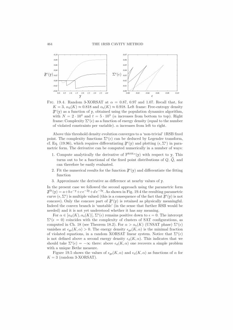
464 THE 1RSB CAVITY METHOD
-0.04
-0.02
0.00
0.02
0.04
0.06
0.08
0.10
0.0 0.5 1.0 1.5 2.0 2.5 3.0 3.5 4.00.00
0.01
0.02
0.03
0.04
0.05
0.06
0.07
0.00 0.02 0.04 0.06 0.08 0.10y ε
Fe(y) Σe(ε)
Fig. 19.4. Random 3-XORSAT at α = 0.87, 0.97 and 1.07. Recall that, forK = 3, αd(K) ≈ 0.818 and αs(K) ≈ 0.918. Left frame: Free-entropy densityFe(y) as a function of y, obtained using the population dynamics algorithm,with N = 2 · 104 and t = 5 · 103 (α increases from bottom to top). Rightframe: Complexity Σe(ε) as a function of energy density (equal to the numberof violated constraints per variable). α increases from left to right.
Above this threshold density evolution converges to a ‘non-trivial’ 1RSB fixedpoint. The complexity functions Σe(ε) can be deduced by Legendre transform,cf. Eq. (19.96), which requires differentiating Fe(y) and plotting (ε,Σe) in para-metric form. The derivative can be computed numerically in a number of ways:
1. Compute analytically the derivative of FRSB,e(y) with respect to y. Thisturns out to be a functional of the fixed point distributions of Q, Q, andcan therefore be easily evaluated.
2. Fit the numerical results for the function Fe(y) and differentiate the fittingfunction
3. Approximate the derivative as difference at nearby values of y.
In the present case we followed the second approach using the parametric formFfit(y) = a+b e−y+c e−2y+d e−3y. As shown in Fig. 19.4 the resulting parametriccurve (ε,Σe) is multiple valued (this is a consequence of the fact that Fe(y) is notconcave). Only the concave part of Fe(y) is retained as physically meaningful.Indeed the convex branch is ‘unstable’ (in the sense that further RSB would beneeded) and it is not yet understood whether it has any meaning.
For α ∈ [αd(K),αs(K)[, Σe(ε) remains positive down to ε = 0. The interceptΣe(ε = 0) coincides with the complexity of clusters of SAT configurations, ascomputed in Ch. 18 (see Theorem 18.2). For α > αs(K) (UNSAT phase) Σe(ε)vanishes at εgs(K,α) > 0. The energy density εgs(K,α) is the minimal fractionof violated equations, in a random XORSAT linear system. Notice that Σe(ε)is not defined above a second energy density εd(K,α). This indicates that weshould take Σe(ε) = −∞ there: above εd(K,α) one recovers a simple problemwith a unique Bethe measure.
Figure 19.5 shows the values of εgs(K,α) and εd(K,α) as functions of α forK = 3 (random 3-XORSAT).

THE NATURE OF 1RSB PHASES 465
0.00
0.05
0.10
0.15
0.20
0.25
0.6 0.8 1 1.2 1.4α
εgs(K,α)
εd(K,α)
Fig. 19.5. Asymptotic ground state energy (= minimal number of violatedconstraints) per variable εgs(K,α) for random K = 3-XORSAT formulae.εgs(K,α) vanishes for α < αs(K). The dashed line εd(K,α) is the highestenergy density e such that configurations with E(x) < Ne are clustered. Itvanishes for α < αd(K).
19.6 The nature of 1RSB phases
In the last sections we discussed how to compute the complexity function Σ(φ)(or its ‘zero temperature’ version, the energetic complexity Σe(ε)). Here we wantto come back to the problem of determining some qualitative properties of themeasure µ( · ) for random graphical models, on the basis of its decompositioninto extremal Bethe measures:
µ(x) =∑
n∈E
wnµn(x) . (19.100)
Assumptions 2 and 3 imply that, in this decomposition, we introduce a neg-ligible error if we drop all the states n but the ones with free-entropy φn ≈ φ∗,where
φ∗ = argmaxφ + Σ(φ) : Σ(φ) ≥ 0 . (19.101)
In general, Σ(φ) is strictly positive and continuous in an interval [φmin,φmax]with Σ(φmax) = 0, and
Σ(φ) = x∗(φmax − φ) + O((φmax − φ)2) , (19.102)
for φ close to φmax.It turns out that the decomposition (19.100) has different properties depend-
ing on the result of the optimization (19.101). One can distinguish two phases(see Fig. 19.6): d1RSB (dynamic one-step replica symmetry breaking) when themax is achieved in the interior of [φmin,φmax] and, as a consequence Σ(φ∗) > 0;s1RSB (static one-step replica symmetry breaking) when the max is achieved atφ∗ = φmax and therefore Σ(φ∗) = 0 (this case occurs iff x∗ ≤ 1).

466 THE 1RSB CAVITY METHOD
φ
Σ
T
T T12
3
φφ3 2 1
Fig. 19.6. A sketch of the complexity Σ versus free-entropy-density φ in afinite-temperature problem with 1RSB phase transition, at three tempera-tures T1 < T2 < T3. A random configuration x with distribution µ(x) isfound with high probability in a cluster of free-entropy-density φ1,φ2,φ3 re-spectively. T2 and T3 are above the condensation transition: φ2,φ3 are thepoints where ∂Σ/∂φ = −1. T1 is below the condensation transition: φ1 is thelargest value of φ where Σ is positive.
19.6.1 Dynamical 1RSB
Assume Σ∗ = Σ(φ∗) > 0. Then we can restrict the sum (19.100) to those statesn such that φn ∈ [φ∗ − ε,φ∗ + ε], if we allow for an exponentially small error.To the leading exponential order there are eNΣ∗ such states whose weights arewn ∈ [e−N(Σ∗+ε′), e−N(Σ∗−ε′)].
Different states are expected to have essentially disjoint support. By this wemean that there exists subsets Ωnn∈E of the configuration space XN such that,for any m ∈ E
µm(Ωm) ≈ 1 ,∑
n∈E\m
wnµn(Ωm) ≈ 0 . (19.103)
Further, different states are separated by ‘large free-energy barriers.’ This meansthat one can choose the above partition in such a way that only an exponentiallysmall (in N) fraction of the probability measure is on its boundaries.
This structure has two important consequences:
Glassy dynamics. Let us consider a local Markov Chain dynamics that sat-isfies detailed balance with respect to the measure µ( · ). As an example we canconsider the Glauber dynamics introduced in Ch. 4 (in order to avoid trivialreducibility effects, we can assume in this discussion that the compatibility func-tions ψa(x∂a) are bounded away from 0).
Imagine initiating the dynamics at time 0 with an equilibrated configurationx(0) distributed according to µ( · ). This is essentially equivalent to picking astate n uniformly at random among the typical ones, and then sampling x(0)from µn( · ). Because of the exponentially large barriers, the dynamics will stayconfined in Ωn for an exponentially large time, and equilibrate among states onlyon larger time scales.

THE NATURE OF 1RSB PHASES 467
This can be formalized as follows. Denote by D(x, x′) the Hamming distancein XN . Take two i.i.d. configuration with distribution µ and let Nd0 be the expec-tation value of their Hamming distance. Analogously take two i.i.d. configurationwith distribution µn, and let Nd1 be the expectation value of their Hammingdistance. When the state n is chosen randomly with distribution wn, we ex-pect d1 not to depend on the state n asymptoticaly for large sizes. Furthermore:d1 < d0. Then we can consider the (normalized) expected Hamming distancebetween configurations at time t in Glauber dynamics d(t) = 〈D(x(0), x(t))〉/N .For any ε < d0−d1, the correlation time τ(ε) ≡ inft : d(t) ≥ d0−ε is expectedto be exponentially large in N
Short-range correlations in finite-dimensional projections. We motivated the1RSB cavity method with the emergence of long-range correlations due to de-composition of µ( · ) into many extremal Bethe measures. Surprisingly, such cor-relations cannot be detected by probing a bounded (when N → ∞) number ofvariables. More precisely, if i(1), . . . , i(k) ∈ 1, · · · , N are uniformly randomvariable indices, then, in the d1RSB phase:
E|〈f1(xi(1))f2(xi(2)) · · · fk(xi(k))〉 − 〈f1(xi(1))〉〈f2(xi(2))〉 · · · 〈fk(xi(k))〉|N→∞→ 0 .
(Here 〈 · 〉 denote the expectation with respect to the measure µ, and E theexpectation with respect to the graphical model in a random ensemble). Thisfinding can be understood intuitively as follows. If there are long range corre-lations among subsets of k variables, then it must be true that conditioning onthe values of k − 1 of them changes the marginal distribution of the k-th one.On the other hand, we think that long range correlations arise because far apartvariables ‘know’ that the whole system is in the same state n. But conditioningon a bounded number (k − 1) of variables cannot select in any significant wayamong the eNΣ∗ relevant states, and thus cannot change the marginal of the k-thone.
An alternative argument makes use of the observation that, if x(1) and x(2) aretwo i.i.d. configurations with distribution µ( · ), then their distance D(x(1), x(2))concentrates in probability. This is due to the fact that the two configurationswill be, with high probability, in different states n1 .= n2 (the probability ofn1 = n2 being e−NΣ∗), whose distance depends weakly on the states couple.
Let us finally notice that the absence of long range correlations among boundedsubset of variables is related to the observation that µ( · ) is itself a Bethe mea-sure (although a non-extremal one) in a d1RSB phase, cf. Sec. 19.4.1. Indeed,each BP equation involves a bounded subset of the variables and can be violatedonly because of correlations among them.
As we shall discuss in Sec. 22.1.2, long range correlations in a d1RSB phasecan be probed through more sophisticated “point-to-set” correlation functions.
19.6.2 Static 1RSB
In this case the decomposition (19.100) is dominated by a few states of near-to-maximal free-entropy φn ≈ φmax. If we ‘zoom’ near the edge by letting φn =
468 THE 1RSB CAVITY METHOD
φmax + sn/N , then the ‘free-entropy shifts’ sn form a point process with densityexp(−x∗s).
The situation is analogous to the one we found in the random energy modelfor T < Tc. Indeed it is expected that the weights wn converge to the sameuniversal Poisson-Dirichlet process found there, and to depend on the model de-tails only through the parameter x∗ (we have already discussed this universalityusing replicas in Ch. 8). In particular, if x(1) and x(2) are two i.i.d. replicas withdistribution µ, and n1, n2 are the states they belong to, then the probability forthem to belong to the same state is
E Pµ(n1 = n2) = E
∑
n∈E
w2n
= 1 − x∗ . (19.104)
Here E denote expectation with respect to the graphical model distribution.As a consequence, the distance D(x(1), x(2)) between two i.i.d. replicas does
not concentrate (the overlap distribution is non-trivial). This in turn can onlybe true if the two-point correlation function does not vanish at large distances.Long-range correlations of this type make BP break down. The original graphicalmodel µ( · ) is no longer a Bethe measure: its local marginals cannot be describedin terms of a set of messages. The 1RSB description, according to which µ( · ) isa convex combination of Bethe measures, is unavoidable.
At this point we are left with a puzzle. How to circumvent the argument givenin Section 19.4.1 that, if the ‘correct’ weight x = 1 is used, then the marginalsas computed within 1RSB still satisfy BP equations? The conundrum is that,within a s1RSB phase, the parameter x = 1 is not the correct one to be used in the1RSB cavity equations (although it is the correct one to weight states). In orderto explain this, let us first notice that, if the complexity is convex and behavesas in Eq. (19.102) near its edge, with a slope −x∗ > −1, then the optimizationproblem (19.101) has the same result as
φ∗ = argmaxxφ + Σ(φ) : Σ(φ) ≥ 0 . (19.105)
for any x ≥ x∗. Therefore, in the 1RSB cavity equations we could in principle useany value of x larger or equal to x∗ (this would select the same states). However,the constraint Σ(φ) ≥ 0 cannot be enforced locally and does not show up inthe cavity equations. If one performs the computation of Σ within the cavitymethod using a value x > x∗, then one finds a negative value of Σ which mustbe rejected (it is believed to be related to the contribution of some exponentiallyrare instances). Therefore, in order to ensure that one studies the interval of φsuch that Σ(φ) ≥ 0, one must impose x ≤ x∗ in the cavity method. In order toselect the states with free-entropy density φmax, we must thus choose the Parisiparameter that corresponds to φmax, namely x = x∗.
19.6.3 When does 1RSB fail?
The 1RSB cavity method is a powerful tool, but does not always provide cor-rect answers, even for locally tree-like models, in the large system limit. The

THE NATURE OF 1RSB PHASES 469
main assumption of the 1RSB approach is that, once we pass to the auxiliarygraphical model (which ‘enumerates’ BP fixed points) a simple BP procedure isasymptotically exact. In other words, the auxiliary problem has a simple ‘replicasymmetric’ structure and no glassy phase. This is correct in some cases, such asrandom XORSAT or SAT close to their SAT-UNSAT threshold, but it may failin others.
A mechanism leading to a failure of the 1RSB approach is that the auxil-iary graphical model is incorrectly described by BP. This may happen becausethe auxiliary model measure decomposes in many Bethe states. In such a case,one should introduce a second auxiliary model, dealing with the multiplicity ofBP fixed points of the first one. This is usually referred to as ‘two-step replicasymmetry breaking’ (2RSB). Obviously one can find situations in which it isnecessary to iterate this construction, leading to a R-th level auxiliary graphicalmodel (R-RSB). Continuous (or full) RSB corresponds to the large-R limit.
While such developments are conceptually clear (at least from an heuristicpoint of view), they are technically challenging. So far limited results have beenobtained beyond 1RSB. For a brief survey, we refer to Ch. 22.
Appendix: SP(y) equations for XORSAT
This appendix provides technical details on the 1RSB treatment of random K-XORSAT, within the ‘energetic’ formalism. The results of this approach werediscussed in Sec. 19.5.4. In particular we will derive the behavior of the auxil-iary free-entropy Fe(y) at large y, and deduce the behavior of the complexityΣe(ε) at small ε. This section can be regarded as an exercise in applying theSP(y) formalism. We shall skip many details and just give the main intermediateresults of the computation.
XORSAT is a constraint satisfaction problems with binary variables. We canthus apply the simplified method of Sec. 19.5.3. The projected min-sum messagescan take three values: 0, 1, ∗. Exploiting the symmetry of XORSAT between 0and 1, SP(y)messages can be parametrized by a single number, e.g. by the sumof their weights on 0 and 1. We will therefore write: Qia(0) = Qia(1) = ζia/2(thus implying Qia(∗) = 1−ζia), and Qai(0) = Qai(1) = ηai/2 (whence Qai(∗) =1 − ηai).
In terms of these variables, the SP(y) equation at function node a reads:
ηai =∏
j∈∂a\i
ζja . (19.106)
The SP(y) equation at variable node i is a bit more complicated. Let usconsider all the |∂i| − 1 incoming messages Qbi, b ∈ ∂i \ a. Each of them isparameterized by a number ηbi. We let η = ηbi, b ∈ ∂i \ a and define thefunction Bq(η) as follows:
Bq(η) =∑
S⊂∂i\a
I(|S| = q)∏
b∈∂i\S∪a
(1 − ηbi)∏
c∈S
ηcj . (19.107)

470 THE 1RSB CAVITY METHOD
Let Aq,r(η) = Bq+r(η)(q+r
q
)2−(q+r). After some thought one obtains the update
equation:
ζia =2∑|∂i|−2
q=0
∑|∂i|−1r=q+1 Aq,r(η)e−yq
∑+(|∂i|−1)/2,q=0 Aq,q(η)e−yq + 2
∑|∂i|−2q=0
∑|∂i|−1r=q+1 Aq,r(η)e−yq
(19.108)
The auxiliary free-entropy FRSB,e(y) has the general form (19.92), with thevarious contributions expressed as follows in terms of the parameters ζia, ηai:
eFRSB,ea = 1 − 1
2(1 − e−y)
∏
i∈∂a
ζia , eFRSB,eai = 1 − 1
2ηaiζia(1 − e−y) ,
eFRSB,ei =
di∑
q=0
di−q∑
r=0
Aq,r (ηaia∈∂i) e−ymin(q,r) . (19.109)
Let us consider random K-XORSAT instances with constraint density α.Equations (19.106), (19.108) get promoted to distributional relations that deter-mine the asymptotic distribution of η and ζ on a randomly chosen edge (i, a).The 1RSB population dynamics algorithm can be used to approximate thesedistributions. We encourage the reader to implement it, and obtain a numericalestimate of the auxiliary free-entropy density Fe(y).
It turns out that, at large y, one can control the distributions of η, ζ ana-lytically, provided their qualitative behavior satisfies the following assumptions(that can be checked numerically):
• With probability t one has η = 0, and with probability 1− t, η = 1− e−yη,where t has a limit in ]0, 1[, and η converges to a random variable withsupport on [0,∞[, as y →∞.
• With probability s one has ζ = 0, and with probability 1−s, ζ = 1−e−yζ,where s has a limit in ]0, 1[, and ζ converges to a random variable withsupport on [0,∞[, as y →∞.
Under these assumptions, we shall expand the distributional version of Eqs. (19.106),(19.108) keeping terms up to first order in e−y. We shall use t, s, η, ζ to denotethe limit quantities mentioned above.
It is easy to see that t, s must satisfy the equations (1 − t) = (1 − s)k−1 ands = e−Kα(1−t). These are identical to Eqs. (19.51) and (19.52), whence t = 1−Q∗and s = 1 −Q∗.
Equation (19.106) leads to the distributional equation:
ηd= ζ1 + · · · + ζK−1 , (19.110)
where ζ1, . . . , ζK−1 are K − 1 i.i.d. copies of the random variable ζ.The update equation (19.108) is more complicated. There are in general l
inputs to a variable node, where l is Poisson with mean Kα. Let us denote by

THE NATURE OF 1RSB PHASES 471
m the number of incoming messages with η = 0. The case m = 0 yields ζ = 0and is taken care of in the relation between t and s. If we condition on m ≥ 1,the distribution of m is
P(m) =λm
m!e−λ
1
1 − e−λI(m ≥ 1) , (19.111)
where λ = Kα(1 − t). Conditional on m, Eq. (19.108) simplifies as follows:
• If m = 1: ζd= η.
• If m = 2: ζ = 1 identically.• If m ≥ 3: ζ = 0 identically.
The various contributions to the free-entropy (19.38) are given by:
fRSB,ef = (1 − s)k
[− log 2 + e−y(1 + K〈ζ〉)
]+ o(e−y) , (19.112)
fRSB,ev =
λ2
2e−λ
[− log 2 + e−y(1 + 2〈η〉)
]
+∞∑
m=3
λm
m!e−λ
[(1 −m) log 2 + e−ym(1 + 〈η〉)
]+ o(e−y) , (19.113)
fRSB,ee = (1 − t)(1 − s)
[− log 2 + e−y(1 + 〈η〉+ 〈ζ〉)
]+ o(e−y) , (19.114)
where 〈η〉 and 〈ζ〉 are the expectation values of η and ζ. This gives for the free-entropy density Fe(y) = fRSB,e
f + αfRSB,ev − Kα fRSB,e
e = Σ0 + e−yε0 + o(e−y),with:
Σ0 =
[1 − λ
k− e−λ
(1 +
k − 1
kλ
)]log 2 , (19.115)
ε0 =λ
k
[1 − e−λ
(1 +
k
2λ
)]. (19.116)
Taking the Legendre transform, cf. Eq. (19.96), we obtain the following behaviorof the energetic complexity as ε → 0:
Σe(ε) = Σ0 + ε logε0e
ε+ o(ε) , (19.117)
This shows in particular that the ground state energy density is proportional to(α−αs)/| log(α−αs)| close to the SAT-UNSAT transition (when 0 < α−αs 8 1).
Exercise 19.7 In the other extreme, show that at large α one gets εgs(K,α) =α/2 +
√2αε∗(K) + o(
√α), where the positive constant ε∗(K) is the absolute
value of the ground state energy of the fully connected K-spin model studiedin Sec. 8.2. This indicates that there is no interesting intermediate asymptoticregime between the M = Θ(N) (discussed in the present chapter) and M =Θ(NK−1) (discussed with the replica method in Ch. 8)

472 THE 1RSB CAVITY METHOD
Notes
The cavity method originated as an alternative to the replica approach in thestudy of the Sherrington-Kirkatrick model (Mezard, Parisi and Virasoro, 1985b).The 1RSB cavity method for locally tree-like factor graphs was developed inthe context of spin glasses in (Mezard and Parisi, 2001). Its application to zerotemperature problems (counting solutions of the min-sum equations), was alsofirst described in the spin glass context in (Mezard and Parisi, 2003). The pre-sentation in this chapter differs in its scope from those work, which were morefocused in computing averages over random instances. For a rigorous treatmentof the notion of Bethe measure, we refer to (Dembo and Montanari, 2008b).
The idea that the 1RSB cavity method is in fact equivalent to applying BP onan auxiliary model appeared in several paper treating the cases of coloring andsatisfiability with y = 0 (Parisi, 2002; Braunstein and Zecchina, 2004; Maneva,Mossel and Wainwright, 2005). The treatment presented here generalizes theseworks, with the important difference that the variables of our auxiliary modelare messages rather than node quantities.
The analysis of the x = 1 case is strictly related to the problem of recon-struction on a tree. This has been studied in (Mezard and Montanari, 2006),where the reader will find the proof of Theorem 19.5 and the expression of thefree-entropy of exercise 19.6.
The SP(y) equations for one single instance have been written first in thecontext of the K-satisfiability problem in (Mezard and Zecchina, 2002), see also(Mezard, Parisi and Zecchina, 2003). The direct derivation of SP(y) equationsin binary variable problems, shown in Sec. 19.5.3, was done originally for satis-fiability in (Braunstein, Mezard and Zecchina, 2005), see also (Braunstein andZecchina, 2004) and (Maneva, Mossel and Wainwright, 2005). The application ofthe 1RSB cavity method to the random XORSAT problem, and its comparisonto the exact results, was done in (Mezard, Ricci-Tersenghi and Zecchina, 2003).
An alternative to the cavity approach followed throughout this book is pro-vided by the replica method of Ch. 8. As we saw, it was first invented in orderto treat fully connected models (i.e. models on complete graphs), cf. (Mezard,Parisi and Virasoro, 1987), and subsequently developed in the context of sparserandom graphs (Mezard and Parisi, 1985; Dominicis and Mottishaw, 1987; Mot-tishaw and Dominicis, 1987; Wong and Sherrington, 1988; Goldschmidt and Lai,1990). The technique was further improved in the paper (Monasson, 1998), thatoffers a very lucid presentation of the method.

20
RANDOM K-SATISFIABILITY
This chapter applies the cavity method to the random K-satisfiability problem.We will study both the phase diagram (in particular, we will determine the SAT-UNSAT threshold αs(K)) and the algorithmic applications of message passing.The whole chapter is based on heuristic derivations: it turns out that the rig-orization of the whole approach is still in its infancy. Neither the conjecturedphase diagram, nor the efficiency of message passing algorithms have been yetconfirmed rigorously. But the computed value of αs(K) is conjectured to be ex-act, and the low-complexity message passing algorithms that we will describeturn out to be particularly efficient in finding solutions.
We will start in Sec. 20.1 by writing the BP equations, following the ap-proach exposed in Ch. 14. The statistical analysis of such equations providesa first (replica symmetric) estimate of αs(K). This however turns out to beincorrect. The reason of this failure is traced back to the incorrectness of thereplica symmetric assumption close to the SAT-UNSAT transition. The systemundergoes a ‘structural’ phase transition at a clause density smaller than αs(K).Nevertheless, BP empirically converges in a wide range of clause densities, andit can be used to find SAT assignments on large instances provided the clausedensity α is not too close to αs(K). The key idea is to use BP as a heuristicguide in a sequential decimation procedure.
In Sec. 20.2 we apply the 1RSB cavity method developed in Ch. 19. Thestatistical analysis of the 1RSB equations gives the values for αs(K) summarizedin Table 20.2.4. From the algorithmic point of view, one can use SP instead of BPas a guide in the decimation procedure. We shall explain and study numericallythe corresponding ‘survey-guided decimation’ algorithm, which is presently themost efficient algorithm to find SAT assignments in large random satisfiableinstances with a clause density close to the threshold αs(K).
This chapter focuses on K-SAT with K ≥ 3. The K = 2 problem is quitedifferent: satisfiability can be proved in polynomial time, the SAT-UNSAT phasetransition is driven by a very different mechanism, and the threshold is knownto be αs(2) = 1. It turns out that a (more subtle) qualitative difference alsodistinguishes K = 3 from K ≥ 4. In order to illustrate this point, we will useboth 3-SAT and 4-SAT as running examples.
Coloring random graphs turns out to be very similar to random K-satisfiability.Section 20.4 presents a few highlights in the study of random graph colorings.In particular, we emphasize how the techniques used for K-satisfiability are suc-cessful in this case as well.
473

474 RANDOM K-SATISFIABILITY
20.1 Belief Propagation and the replica symmetric analysis
We already studied some aspects of random K-SAT in Ch. 10, where we derivedin particular some rigorous bounds on the SAT/UNSAT threshold αs(K). Herewe will study the problem using message passing approaches. Let us start bysummarizing our notations.
An instance of the K-satisfiability problem is defined by M clauses (indexedby a, b · · · ∈ 1, . . . , M) over N Boolean variables x1, . . . , xN taking values in0, 1. We denote by ∂a the set of variables in clause a, and by ∂i the set ofclauses in which variable xi appears. Further, for each i ∈ ∂a, we introduce thenumber Jai which takes value 1 if xi appears negated in clause a, and takes value0 if the variable appears unnegated.
It will be convenient to distinguish elements of ∂a according to the values ofJai. We let ∂0a ≡ i ∈ ∂a s.t. Jai = 0 and ∂1a = i ∈ ∂a s.t. Jai = 1. Similarlywe denote by ∂0i and ∂1i the neighborhoods of i: ∂0i = a ∈ ∂i s.t. Jai = 0 and∂1i = a ∈ ∂i s.t. Jai = 1.
As usual, the indicator function over clause a being satisfied is denoted byψa( · ): ψa(x∂a) = 1 if clause a is satisfied by the assignment x and ψa(x∂a) = 0if it is not. Given a SAT instance, we begin by studying the uniform measureover SAT assignments:
µ(x) =1
Z
M∏
a=1
ψa(x∂a) . (20.1)
We will represent this distribution with a factor graph, as in Fig. 10.1, and inthis graph we draw dashed edges when Jai = 1, and full edges when Jai = 0.
20.1.1 The BP equations
The BP equations for a general model of the form (20.1) have already beenwritten in Chapter 14. Here we want to rewrite them in a more compact form,that is convenient both for analysis and implementation. They are best expressedusing the following notation. Consider a variable node i connected to factor nodea and partition its neighborhood as ∂i = a ∪ Sia ∪ Uia, where (see Fig. 20.1):
if Jai = 0 then Sia = ∂0i \ a, Uia = ∂1i ,
if Jai = 1 then Sia = ∂1i \ a, Uai = ∂0i . (20.2)
Since the variables xi’s are binary, the BP messages at any time νi→a( · ),νa→i( · ), can be parameterized by a single real number. We fix the parameteri-zation by letting ζia ≡ νi→a(xi = Jai) (which obviously implies νi→a(xi = 1 −Jai) = 1− ζia), and ζai ≡ νa→i(xi = Jai) (yielding νa→i(xi = 1−Jai) = 1− ζai).
A straightforward calculation allows to express the BP equations (here infixed point form) in terms of these variables:

BELIEF PROPAGATION AND THE REPLICA SYMMETRIC ANALYSIS 475
ij
a
Sia
Uia
Uja
Sja
Fig. 20.1. The set Sia contains all checks b in ∂i \ a such that Jbi = Jai, theset Uia contains all checks b in ∂i \ a such that Jbi = 1 − Jai
ζia =
[∏b∈Sia
ζbi
] [∏b∈Uia
(1 − ζbi)]
[∏b∈Sia
ζbi
] [∏b∈Uia
(1 − ζbi)]
+[∏
b∈Uiaζbi
] [∏b∈Sia
(1 − ζbi)] ,
ζai =1 −
∏j∈∂a\i ζja
2 −∏
j∈∂a\i ζja, (20.3)
with the convention that a product over zero term is equal to 1. Notice that eval-uating the right hand side takes (respectively) O(|∂i|) and O(|∂a|) operations.This should be contrasted with the general implementation of the BP equations,cf. Ch. 14 , that requires O(|∂i|) operations at variable nodes but O(2|∂a|) atfunction nodes.
The Bethe free-entropy takes the usual form, cf. Eq. (14.27), F =∑
a∈F Fa +∑i∈V Fi −
∑(ia)∈E Fia. The various contributions can be expressed in terms of
the parameters ζia, ζai as follows
Fa = log
[1 −
∏
i∈∂a
ζia
]; Fi = log
[∏
a∈∂0i
ζai
∏
b∈∂1i
(1 − ζbi) +∏
a∈∂0i
(1 − ζai)∏
b∈∂1i
ζbi
];
Fai = log[(1 − ζia)(1 − ζai) + ζiaζai
]. (20.4)
Given the messages, the BP estimate for the marginal on site i is:
νi(xi) ∼=∏
a∈∂i
νa→i(xi) . (20.5)
20.1.2 Statistical analysis
Let us now consider a random K-sat formula, i.e. a uniformly random formulawith N variables and M = Nα clauses. The resulting factor graph will be dis-

476 RANDOM K-SATISFIABILITY
tributed according to the GN (K, M) ensemble. Given a variable index i, thenumbers |∂0i|, |∂1i| of variables in which xi appears directed or negated, con-verge to independent Poisson random variables of mean Kα/2.
If (i, a) is a uniformly random edge in the graph, the corresponding fixed pointmessages ζia, ζai are random variables (we assume here that an ‘approximate’fixed point exists). Within the RS assumption, they converge in distribution, asN →∞, to random variables ζ, ζ whose distribution satisfy the RS distributionalequations
ζd=
1 − ζ1 . . . ζK−1
2 − ζ1 . . . ζK−1, (20.6)
ζd=
ζ1 . . . ζp(1 − ζp+1) . . . (1 − ζp+q)
ζ1 . . . ζp(1 − ζp+1) . . . (1 − ζp+q) + (1 − ζ1) . . . (1 − ζp)ζp+1 . . . ζp+q
. (20.7)
Here p and q are two i.i.d. Poisson random variables with mean Kα/2 (cor-responding to the sizes of S and U), ζ1, . . . , ζK−1 are i.i.d. copies of ζ, andζ1, . . . , ζp+q are i.i.d. copies ζ.
The distributions of ζ and ζ can be approximated using the population dy-namics algorithm. The resulting samples can then be used to estimate the free-entropy density, as outlined in the exercise below.
Exercise 20.1 Argue that, within the RS assumptions, the large N limit ofthe Bethe free-entropy density is given by limN→∞ F/N = fRS = fRS
v + αfRSc −
KαfRSe , where:
fRSv = E log
[p∏
a=1
ζa
p+q∏
a=p+1
(1 − ζa) +p∏
a=1
(1 − ζa)p+q∏
a=p+1
ζa
],
fRSc = E log [1 − ζ1 · · · ζK−1] ,
fRSe = E log
[(1 − ζ1)(1 − ζ1) + ζ1ζ1
]. (20.8)
Here E denotes the expectation with respect to: ζ1, . . . , ζK which are i.i.d.copies of ζ; ζ1, . . . , ζp+q which are i.i.d. copies of ζ; p and q which are i.i.d.Poisson random variables with mean Kα/2.
Fig. 20.2 shows an example of the entropy density found within this approachfor 3-SAT. For each value of α in a mesh, we used a population of size 104, andran the algorithm for 3·103 iterations. Messages are initialized uniformly in ]0, 1[,and the first 103 iterations are not used for computing the free-entropy.
The predicted entropy density is strictly positive and decreasing in α forα ≤ α∗(K), with α∗(3) ≈ 4.6773. Above α∗(K) the RS distributional equationsdo not seem to admit any solution with ζ, ζ ∈ [0, 1]. This is revealed numericallyby the fact that the denominator of Eq. (20.7) vanishes during the populationupdates. Since one finds a RS entropy density which is positive for all α < α∗(K),
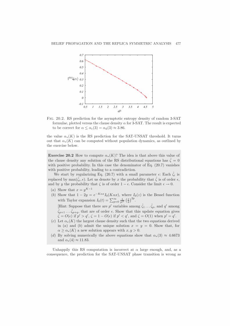
BELIEF PROPAGATION AND THE REPLICA SYMMETRIC ANALYSIS 477
-0.1
0
0.1
0.2
0.3
0.4
0.5
0.6
0.7
0.5 1 1.5 2 2.5 3 3.5 4 4.5 5
S
α
fRS(α)
α
Fig. 20.2. RS prediction for the asymptotic entropy density of random 3-SATformulae, plotted versus the clause density α for 3-SAT. The result is expectedto be correct for α ≤ αc(3) = αd(3) ≈ 3.86.
the value α∗(K) is the RS prediction for the SAT-UNSAT threshold. It turnsout that α∗(K) can be computed without population dynamics, as outlined bythe exercise below.
Exercise 20.2 How to compute α∗(K)? The idea is that above this value ofthe clause density any solution of the RS distributional equations has ζ = 0with positive probability. In this case the denominator of Eq. (20.7) vanisheswith positive probability, leading to a contradiction.
We start by regularizing Eq. (20.7) with a small parameter ε: Each ζi isreplaced by max(ζi, ε). Let us denote by x the probability that ζ is of order ε,and by y the probability that ζ is of order 1− ε. Consider the limit ε → 0.
(a) Show that x = yK−1
(b) Show that 1 − 2y = e−KαxI0(Kαx), where I0(z) is the Bessel function
with Taylor expansion I0(t) =∑∞
p=01
p!2
(t2
)2p.
[Hint: Suppose that there are p′ variables among ζ1 . . . ζp, and q′ among
ζp+1 . . . ζp+q, that are of order ε. Show that this update equation givesζ = O(ε) if p′ > q′, ζ = 1 −O(ε) if p′ < q′, and ζ = O(1) when p′ = q′.
(c) Let α∗(K) the largest clause density such that the two equations derivedin (a) and (b) admit the unique solution x = y = 0. Show that, forα ≥ α∗(K) a new solution appears with x, y > 0.
(d) By solving numerically the above equations show that α∗(3) ≈ 4.6673and α∗(4) ≈ 11.83.
Unhappily this RS computation is incorrect at α large enough, and, as aconsequence, the prediction for the SAT-UNSAT phase transition is wrong as
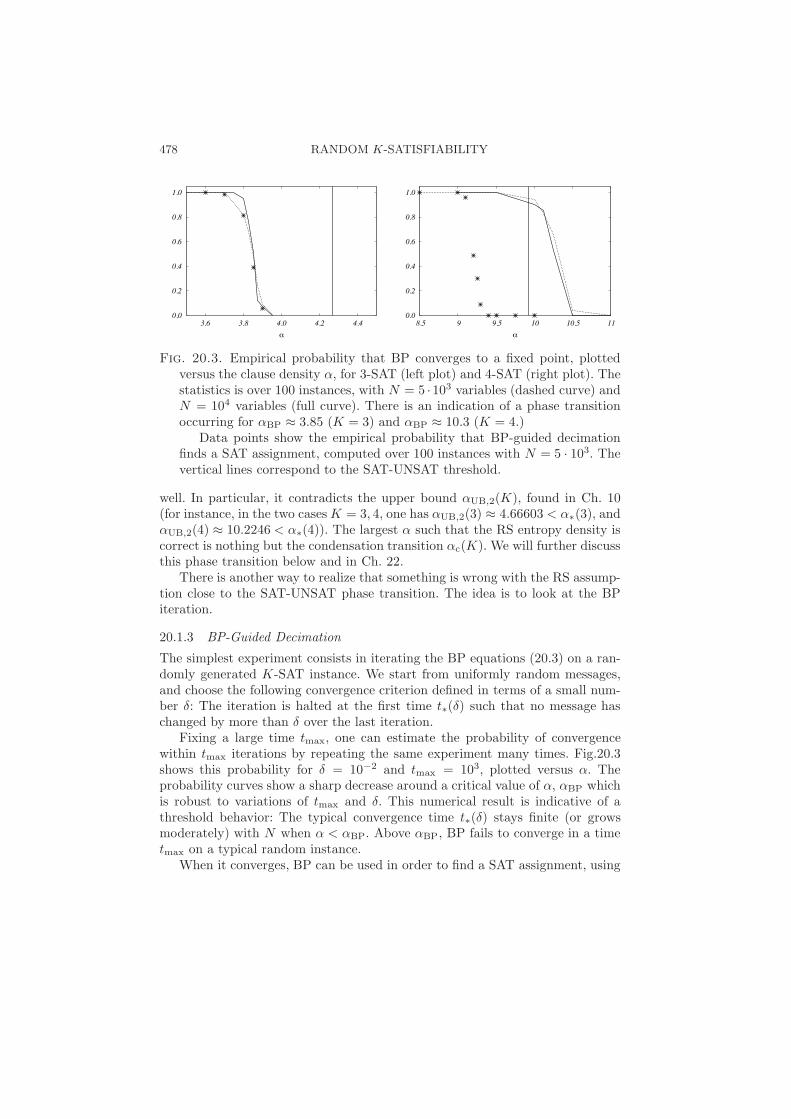
478 RANDOM K-SATISFIABILITY
0.0
0.2
0.4
0.6
0.8
1.0
3.6 3.8 4.0 4.2 4.4α
0.0
0.2
0.4
0.6
0.8
1.0
8.5 9 9.5 10 10.5 11α
Fig. 20.3. Empirical probability that BP converges to a fixed point, plottedversus the clause density α, for 3-SAT (left plot) and 4-SAT (right plot). Thestatistics is over 100 instances, with N = 5 ·103 variables (dashed curve) andN = 104 variables (full curve). There is an indication of a phase transitionoccurring for αBP ≈ 3.85 (K = 3) and αBP ≈ 10.3 (K = 4.)
Data points show the empirical probability that BP-guided decimationfinds a SAT assignment, computed over 100 instances with N = 5 · 103. Thevertical lines correspond to the SAT-UNSAT threshold.
well. In particular, it contradicts the upper bound αUB,2(K), found in Ch. 10(for instance, in the two cases K = 3, 4, one has αUB,2(3) ≈ 4.66603 < α∗(3), andαUB,2(4) ≈ 10.2246 < α∗(4)). The largest α such that the RS entropy density iscorrect is nothing but the condensation transition αc(K). We will further discussthis phase transition below and in Ch. 22.
There is another way to realize that something is wrong with the RS assump-tion close to the SAT-UNSAT phase transition. The idea is to look at the BPiteration.
20.1.3 BP-Guided Decimation
The simplest experiment consists in iterating the BP equations (20.3) on a ran-domly generated K-SAT instance. We start from uniformly random messages,and choose the following convergence criterion defined in terms of a small num-ber δ: The iteration is halted at the first time t∗(δ) such that no message haschanged by more than δ over the last iteration.
Fixing a large time tmax, one can estimate the probability of convergencewithin tmax iterations by repeating the same experiment many times. Fig.20.3shows this probability for δ = 10−2 and tmax = 103, plotted versus α. Theprobability curves show a sharp decrease around a critical value of α, αBP whichis robust to variations of tmax and δ. This numerical result is indicative of athreshold behavior: The typical convergence time t∗(δ) stays finite (or growsmoderately) with N when α < αBP. Above αBP, BP fails to converge in a timetmax on a typical random instance.
When it converges, BP can be used in order to find a SAT assignment, using

BELIEF PROPAGATION AND THE REPLICA SYMMETRIC ANALYSIS 479
it as an heuristic guide for a sequential decimation procedure. Each time thevalue of a new variable has to be fixed, BP is iterated until the convergencecriterion, with parameter δ, is met (alternatively, one may be more bold and usethe BP messages after a time tmax even when they have not converged). Thenone uses the BP messages in order to decide: (i) Which variable to fix; (ii) Whichvalue should the variable take.
In the present implementation these decisions are taken on the basis of asimple statistics: the variables bias. Given the BP estimate νi( · ) of the marginalof xi, we define the bias as πi ≡ νi(0) − νi(1).
BP-Guided Decimation (SAT formula F , Accuracy ε, Iterations tmax)1: For all n ∈ 1, . . . , N:2: Call BP(F ,ε, tmax);3: If BP does not converge, return ‘NOT found’ and exit;4: For each variable node j, compute the bias πj ;5: Find a variable i(n) with the largest absolute bias |πi(n)|;6: If πi(n) ≥ 0, fix xi(n) to x∗
i(n) = 0;
7: Otherwise, fix xi(n) to x∗i(n) = 1;
8: Replace F by the formula obtained after this reduction8: End-For;10: Return the assignment x∗
A pseudocode for BP was given in Sec. 14.2. Let us emphasize that the samedecimation procedure could be used not only with BP, but with other types ofguidance, as soon as we have some way to estimate the marginals.
The empirical success probability of the BP-Guided decimation on randomformulae are shown in Fig. 20.3 (estimated from 100 instances of size N = 5 ·104)for several values of α. The qualitative difference between 3-SAT and 4-SATemerges clearly from this data. In 3-SAT, the decimation procedure returns aSAT assignment about every time it converges, i.e. with probability close to onefor α " 3.85. In 4-SAT, BP converges most of the times if α " 10.3. This valueis larger than the conjectured SAT-UNSAT threshold αs(4) ≈ 9.931 (and alsolarger than the best rigorous upper bound αUB,2(4) ≈ 10.2246.) On the otherhand, the BP guided decimation finds SAT assignments only when α " 9.25. Itis believed that the cases K ≥ 5 behave as K = 4.
20.1.4 On the validity of the RS analysis
These experiments suggest that something is not correct in the RS assumptionsfor α large enough. The precise mechanism by which they are incorrect dependshowever on the value of K. For K = 3, the BP fixed point become unstable,and this leads to errors in decimations. In fact, the local stability of the BP fixedpoint can be computed along the lines of Sec. 17.4.2. The result is that it becomeunstable at αst(3) ≈ 3.86. On the contrary, for K ≥ 4 the fixed point remainsstable but does not correspond to the correct marginals. Local stability is not a
480 RANDOM K-SATISFIABILITY
good enough test in this case.Correspondingly, one can define two type of thresholds:
(i) A stability threshold αst(K) beyond which BP does not have a locallystable fixed point.
(ii) A 1RSB condensation threshold αc(K) beyond which there is no BP fixedpoint giving a correct estimate of the local marginals and free-entropy.
One should clearly have αc(K) ≤ αst(K). Our study suggests that αc(3) =αst(3) 1 3.86 while, for K ≥ 4, one has a strict inequality αc(K) < αst(K).
The reason for the failure of BP is the decomposition of the measure (20.1) inmany pure states. This happens at a third critical value αd(K) ≤ αc(K), referredto as the dynamical transition, in accordance with our discussion of spin glassesin Sec. 12.3: αd(K) is the critical clause density above which Glauber dynamicswill become inefficient. If αd(K) < α < αc(K), one expects, as we discussed inSec. 19.4.1, that there exist many pure states, and many quasi-solutions to BPequations among which one will give the correct marginals.
At this point the reader might well be discouraged. This is understandable:we started seeking one threshold (the SAT-UNSAT transition αs(K)) and rapidlyended up defining a number of other thresholds, αd(K) ≤ αc(K) ≤ αst(K) ≤αs(K) to describe a zoology of exotic phenomena. It turns out that, while theunderstanding of the proliferation of pure states is necessary to get the correctvalue of αs(K), one does not need a detailed description of the clusters, which is achallenging task. Luckily, there exists a shortcut, through the use of the energeticcavity method. It turns out that the sketchy description of clusters that we getfrom this method, as if looking at them from far, is enough to determine αs.Even more than that. The sketch will be a pretty useful and interesting one.In Sec. 20.3, we will discuss a more detailed picture obtained through the full-fledged 1RSB cavity method applied to the model (20.1).
20.2 Survey propagation and the 1RSB phase
The use of the energetic 1RSB cavity method can be motivated in two ways. Froma first point of view, we are changing problem. Instead of computing marginalsof the distribution (20.1), we consider the problem of minimizing the energyfunction
E(x) =M∑
a=1
Ea(x∂a) . (20.9)
Here Ea(x∂a) = 0 if clause a is satisfied by the assignment x, and Ea(x∂a) = 1otherwise. The SAT-UNSAT threshold αs(K) is thus identified as the criticalvalue above which the ground state energy minE(x) vanishes.
With the cavity method we shall estimate the ground state energy density,and find that it vanishes below some threshold. This is then identified as αs(K).This identification amounts to assuming that, for generic large random K-SATproblems, there is no interval of α where the ground state energy is positive but
SURVEY PROPAGATION AND THE 1RSB PHASE 481
sub-linear in N . This assumption is reasonable, but of course it does not hold inmore general situations. If, for instance, we added to a random K-SAT formula asmall unsatisfiable sub-formula (including o(N) variables), our approach wouldnot detect the change, while the formula would be always unsatisfiable.
For α < αs(K) the cavity method provides a rough picture of zero energy purestates. This brings us to the second way of motivating this ‘sketch.’ We saw thatdescribing a pure (Bethe) state in a locally tree-like graph amounts to assigninga set of cavity messages, i.e. of marginal distributions for the variables. Thesimplified description of the energetic 1RSB method only distinguishes betweenmarginals that are concentrated on a single value, and marginals that are not.The concentrated marginals are described exactly, while the other ones are justsummarized by a single statement, “not concentrated”.
20.2.1 The SP(y) equations
The satisfiability problem involves only hard constraints and binary variables.We can thus use the simplified SP(y) equations of Sec. 19.5.3. The messages aretriples: (Qia(0), Qia(1), Qia(∗)) for variable-to-function messages, and (Qai(0), Qai(1), Qai(∗))for function-to-variable messages.
In the case of K-satisfiability, these can be further simplified. The basic ob-servation is that, if Jai = 0 then Qai(1) = 0, and if Jai = 1 then Qai(0) = 0.This can be shown either starting from the general formalism in Sec. 19.5.3, orreconsidering the interpretation of warning propagation messages. Recall that a“0” message means that the constraint a ‘forces’ variable xi to take value 0 inorder to minimize the system’s energy. In K-SAT this can happen only if Jai = 0,because xi = 0 is then the value that satisfies the clause a. With this remark inmind, the function-to-variable node message can be parameterized by a singlereal number. We will choose it to be Qai(0) if Jai = 0, and Qai(1) if Jai = 1 ,and we shall denote it as Qai. This number Qai is the probability that there isa warning sent from a to i which forces the value of variable xi.
Analogously, it is convenient to adopt a parameterization of the variable-to-function message Qia(m) which takes into account the value of Jai. Precisely,recall that Qia is supported on three types of messages: m(0) = 0, m(1) > 0, orm(0) = m(1) = 0, or m(0) > 0, m(1) = 0. Let us denote the corresponding weightsas Qia(0), Qia(∗), Qia(1). If Jai = 0, we then define QS
ia ≡ Qia(0), Q∗ia ≡ Qia(∗)
and QUia ≡ Qia(1). Vice-versa, if Jai = 1, we let QS
ia ≡ Qia(1), Q∗ia ≡ Qia(∗) and
QUia ≡ Qia(0).
Below we summarize these notations with the corresponding interpretations.We emphasize that ‘probability’ refers here to the random choice of a pure state,cf. Sec. 19.1.
482 RANDOM K-SATISFIABILITY
QSia: probability that xi is forced by the clauses b ∈ ∂i \ a to satisfy a,
QUia: probability that xi is forced by the clauses b ∈ ∂i \ a to violate a,
Q∗ia: probability that xi is not forced by the clauses b ∈ ∂i \ a.
Qai: probability that xi is forced by clause a to satisfy it.
The 1RSB cavity equations have been written in Sec. 19.5.3.
Exercise 20.3 Write explicitly the 1RSB equations in terms of the messagesQS, QU, Q∗, Q applying the procedure of Sec. 19.5.3.
Alternatively, they can be guessed having in mind the above interpretation.Clause a forces variable xi to satisfy it if and only if all the other variablesentering clause a are forced (by some other clause) not to satisfy a. This means:
Qai =∏
j∈∂a\i
QUja . (20.10)
Consider on the other hand variable node i, and assume for definiteness thatJia = 0 (the opposite case gives rise to identical equations). Remember that, inthis case, Sia denotes the subset of clauses b .= a in which Jib = 0, and Uia thesubset in which Jib = 1. Assume that the clauses in ΩS ⊆ Sia, and ΩU ⊆ Uia forcexi to satisfy them. Then xi is forced to satisfy or violate a depending whether|ΩS| > |ΩU| or |ΩS| < |ΩU|. Finally, xi is not forced if |ΩS| = |ΩU|. The energyshift is equal to the number of ‘forcing’ clauses in ∂i \ a that are violated whenxi is chosen to satisfy the largest number of them, namely min(|ΩU|, |ΩS|). Wethus get the equations
QUia∼=
∑
|ΩU|>|ΩS|
e−y|ΩS|∏
b∈ΩU∪ΩS
Qbi
∏
b-∈ΩU∪ΩS
(1 − Qbi) , (20.11)
QSia∼=
∑
|ΩS|>|ΩU|
e−y|ΩU|∏
b∈ΩU∪ΩS
Qbi
∏
b-∈ΩU∪ΩS
(1 − Qbi) , (20.12)
Q∗ia∼=
∑
|ΩU|=|ΩS|
e−y|ΩU|∏
b∈ΩU∪ΩS
Qbi
∏
b-∈ΩU∪ΩS
(1 − Qbi) . (20.13)
The overall normalization is fixed by the condition QUia + Q∗
ia + QSia = 1.
As usual, Eqs (20.10-20.13) can be understood either as defining a map-ping from the space of messages Qai, Qia onto itself or as a set of fixed pointconditions. In both cases they are referred to as the SP(y) equations for thesatisfiability problem. From the computational point of view, these equationsinvolve a sum over 2|∂i|−1 terms. This is often too much if we want to iteratethe SP(y) equations on large K-SAT formulae: the average degree of a variablenode in a random K-SAT formula with clause density α is Kα. Further, in themost interesting regime –close to the SAT-UNSAT threshold– α = Θ(2K), and

SURVEY PROPAGATION AND THE 1RSB PHASE 483
the sum is over 2Θ(K2K) terms, which becomes rapidly unpractical. It is thusimportant to notice that the sums can be computed efficiently by interpretingthem as convolutions.
Exercise 20.4 Consider a sequence of independent Bernoulli random variablesX1, . . . , Xn, . . . , with means (respectively) η1, . . . , ηn, . . . . Let Wn(m) be theprobability that the sum
∑nb=1 Xb is equal to m.
(a) Show that these probabilities satisfy the recursion
Wn(m) = ηnWn−1(m − 1) + (1 − ηn)Wn−1(m) ,
for m ∈ 0, . . . , n. Argue that these identities can be used together withthe initial condition W0(m) = I(m = 0), to compute Wn(m) in O(n2)operations.
(b) How can one compute the right hand sides of Eqs. (20.11-20.13) inO(|∂i|2) operations?
20.2.2 The free-entropy FRSB,e
Within the 1RSB energetic cavity method, the free-entropy FRSB,e(Q, Q) pro-vides detailed information on the minimal energy of (Bethe) pure states. Thesepure states are nothing but metastable minima of the energy function (i.e. min-ima whose energy cannot be decreased with a bounded number of spin flips).
The 1RSB free-entropy is expressed in terms of a set of messages Qia, Qaithat provide a (quasi-)solution of the SP(y) equations (20.10-20.13). Followingthe general theory in Sec. 19.5.2, it can be written in the form
FRSB,e(Q, Q) =∑
a∈C
FRSB,ea +
∑
i∈V
FRSB,ei −
∑
(i,a)∈E
FRSB,eia . (20.14)
Equation (19.95) yields
eFRSB,eia = 1 − (1 − e−y)QaiQ
Uia . (20.15)
The contribution FRSB,ea defined in (19.93) can be computed as follows. The
reweighting Fea(mia) is always equal to 0, except for the case where all the
variables in clause a receive a warning requesting that they point in the “wrongdirection”, namely the direction which does not satisfy the clause. Therefore:
eFRSB,ea = 1 − (1 − e−y)
∏
i∈∂a
QUia .
Finally, the contribution FRSB,ei defined in (19.94) depends on the messages sent
from check nodes b ∈ ∂i. Let us denote by ΩS ⊆ ∂0i the subset of check nodes
484 RANDOM K-SATISFIABILITY
b ∈ ∂0i such that clause b forces xi to satisfy it. Similarly, defined as ΩU ⊆ ∂1ithe subset of ∂1i such that clause b forces xi to satisfy it. We then have:
eFRSB,ei =
∑
ΩU,ΩS
e−ymin(ΩS,ΩU)
[∏
b∈ΩU∪ΩS
Qbi
]
∏
b-∈ΩU∪ΩS
(1 − Qbi)
. (20.16)
Exercise 20.5 Show that, for any i ∈ ∂a, FRSB,eia = FRSB,e
a .
20.2.3 Large y limit: the SP equations
Consider now the case of satisfiable instances. A crucial problem is then tocharacterize satisfying assignments and to find them efficiently. This amountsto focusing on zero energy assignments, which are selected by taking the y →∞limit within the energetic cavity method.
We can take the limit y → ∞ in the SP(y) equations (20.11-20.13). Thisyields
Qai =∏
j∈∂a\i
QUja , (20.17)
QUja
∼=∏
b∈Sja
(1 − Qbj)
1 −∏
b∈Uja
(1 − Qbj)
, (20.18)
QSja
∼=∏
b∈Uja
(1 − Qbj)
1 −∏
b∈Sja
(1 − Qbj)
, (20.19)
Q∗ja
∼=∏
b∈∂j\a
(1 − Qbj) , (20.20)
where the normalization is always fixed by the condition QUja + QS
ja + Q∗ja = 1.
The y = ∞ equations have a simple interpretation. Consider a variable xj
appearing in clause a, and assume it receives a warning from clause b .= a in-dependently with probability Qbj . Then
∏b∈Sja
(1− Qbj) is the probability thatvariable j receives no warning forcing it in the direction which satisfies clausea. The product
∏b∈Uja
(1 − Qbj) is the probability that variable j receives no
warning forcing it in the direction which violates clause a. Therefore QUja is the
probability that variable j receives at least one warning forcing it in the directionwhich violates clause a, conditional to the fact that there are no contradictions inthe warnings received by j from clauses b .= a. Analogous interpretations hold forQS
ja and Q∗ja. Finally, Qai is the probability that all variables in ∂a\ i are forced
in the direction violating clause a, under the same condition of no contradiction.Notice that the y = ∞ equations are a relatively simple modification of
the BP equations in (20.3). However, the interpretation of the messages is verydifferent in the two cases.

SURVEY PROPAGATION AND THE 1RSB PHASE 485
Finally the free-entropy in the y = ∞ limit is obtained as
FRSB,e =∑
a∈C
FRSB,ea +
∑
i∈V
FRSB,ei −
∑
(i,a)∈E
FRSB,eia , (20.21)
where
FRSB,eia = log
1 −QU
iaQai
, (20.22)
FRSB,ei = log
∏
b∈∂0i
(1 − Qbi) +∏
b∈∂1i
(1 − Qbi) −∏
b∈∂i
(1 − Qbi)
, (20.23)
FRSB,ea = log
1 −∏
j∈∂a
QUja
. (20.24)
Exercise 20.6 Show that, if the SP messages satisfy the fixed point equations(20.17) to (20.20), the free-entropy can be rewritten as FRSB,e =
∑i FRSB,e
i +∑a(1 − |∂a|)FRSB,e
a .
20.2.4 The SAT-UNSAT threshold
The SP(y) equations (20.10-20.13) always admit a ‘no warning’ fixed point corre-sponding to Qai = 0, and QS
ia = QUia = 0, Q∗
ia = 1 for each (i, a) ∈ E. Other fixedpoints can be explored numerically by iterating the equations on large randomformulae.
Within the cavity approach, the distribution of the message associated to auniformly random edge (i, a) satisfies a distributional equation. As explained inSec. 19.2.5, this distributional equation is obtained by promoting Qai, (QU
ia, QSia, Q∗
ia)to random variables and reading Eqs. (20.10-20.13) as equalities in distribution.The distribution can then be studied by the population dynamics of Sec. 19.2.6. Itobviously admits a no-warning (or ‘replica symmetric’) fixed point, with Q = 0,(QU, QS, Q∗) = (0, 0, 1) identically, but (as we will see) in some cases one alsofinds a different, ‘non-trivial’ fixed point distribution.
Given a fixed point, the 1RSB free-entropy density Fe(y) is estimated by tak-ing the expectation of Eq. (20.14) (both with respect to degrees and fields) anddividing by N . When evaluated on the no-warning fixed point, the free-entropydensity Fe(y) vanishes. This means that the number of clusters of SAT assign-ments is sub-exponential, so that the corresponding complexity density vanishes.To a first approximation, this solution corresponds to low-energy assignmentsforming a single cluster. Note that the energetic cavity method counts the num-ber of clusters of SAT assignments, and not the number of SAT assignmentsitself (which is actually exponentially large).
Figure 20.4 shows the outcome of a population dynamics computation. Weplot the free-entropy density Fe(y) as a function of y for random 3-SAT, ata few values of the clause density α. These plots are obtained initializing the

486 RANDOM K-SATISFIABILITY
-0.005
0
0.005
0.01
0.015
0.02
0 1 2 3 4 5 y
Fe(y)
Fig. 20.4. 1RSB free-entropy density for 3-SAT, computed from the populationdynamics analysis of the SP equation, at α = 4.1, 4.2, 4.3 (from top tobottom). For each α, y, a population of size 12000 has been iterated 12 · 106
times. The resulting Fe has been computed by averaging over the last 8 · 106
iterations.
population dynamics recursion with i.i.d. messages Qi uniformly random in[0, 1]. For α < αd,SP 1 3.93, the iteration converges to the ‘no-warning’ fixed
point where all the messages Q are equal to 0.For α > αd,SP , and when y is larger than a critical value yd(α) the iteration
converges to a non-trivial fixed point. This second solution has a non-vanishingvalue of the free-entropy density Fe(y). The energetic complexity Σe(ε) is ob-tained from Fe(y) via the Legendre transform (19.96).
In practice, the Legendre transform is computed by fitting the population dy-namics data, and then transforming the fitting curve. Good results are obtainedwith a fit of the form Fe
fit(y) =∑r∗
r=0 ψr e−ry with r∗ between 2 and 4. Theresulting curves Σe(ε) (or more precisely their concave branches30) are shown inFig. 20.5.
Exercise 20.7 Show that Σe(ε = 0) = limy→∞ Fe(y)
The energetic complexity Σe(ε) is the exponential growth rate number of(quasi-)solutions of the min-sum equations with energy density u. As can beseen in Fig. 20.5, for α = 4.1 or 4.2 (and in general, in an interval above αd(3))one finds Σe(ε = 0) > 0. The interpretation is that there exist exponentiallymany solutions of the min-sum equations with zero energy density.
On the contrary when α = 4.3 the curve starts at a positive ε or, equivalentlythe 1RSB complexity curve has Σe(ε = 0) < 0. Of course, the typical number
30Σe(ε) has a second, convex branch which joins the concave part at the maximal value ofε; the precise meaning of this second branch is not known.

SURVEY PROPAGATION AND THE 1RSB PHASE 487
0.001 0.002 0.003 0.004 0.005
0.01
0.02
ε
Σe(ε)
Fig. 20.5. Energetic complexity density Σe plotted versus energy density ε,for the 3-SAT problem at α = 4.1, 4.2, 4.3 (from top to bottom). Thesecurves have been obtained as the Legendre transform of the free-entropy fitsof Fig. 20.4.
of min-sum solutions cannot decrease exponentially. The result Σe(ε = 0) < 0 isinterpreted as a consequence of the fact that a typical random formula does notadmit any (approximate) solution of the min-sum equations with energy densityε = 0. Given the correspondence between min-sum fixed points and clusters oflow-energy assignments, this in turns implies that a typical random formula doesnot have any SAT assignment.
From Fig. 20.5 one expects that the SAT-UNSAT transition lies between α =4.2 and α = 4.3. A more precise estimate can be obtained by plotting Fe(y →∞)versus α, and locating the value of α where it vanishes. For 3-SAT one obtainsthe SAT-UNSAT threshold estimate αs(3) = 4.26675± 0.00015. The predictionsof this method for αs(K) are shown in the Table 20.2.4. In practice, reliableestimates can be obtained with population dynamics only for K ≤ 7. The reasonis that αs(K) increases exponentially with K, and the size of the populationneeded in order to achieve a given precision should increase accordingly (theaverage number of independent messages entering the distributional equations isKα).
For large K, one can formally expand the distributional equations, whichyields a series for αs(K) in powers of 2−K . The first two terms (seven terms havebeen computed) of this expansion are:
αs(K) = 2K log 2 − 1
2(1 + log 2) + O(2−KK2) (20.25)
20.2.5 SP-Guided Decimation
The analysis in the last few pages provides a refined description of the set ofsolutions of random formulae. This knowledge can be exploited to efficiently

488 RANDOM K-SATISFIABILITY
K 3 4 5 6 7 8 9 10αs(K) 4.2667 9.931 21.117 43.37 87.79 176.5 354.0 708.9
Table 20.1 Predictions of the 1RSB cavity method for the SAT-UNSAT thresh-old of random K satisfiability
find some solutions, much in the same way as we used belief propagation inSec. 20.1.3. The basic strategy is again to use the information provided by theSP messages as a clever heuristic in a decimation procedure.
The first step consists in finding an approximate solution of the SP(y) equations(20.10-20.13), or of their simplified y = ∞ version (20.17-20.20), on a given in-stance of the problem. To be definite, we shall focus on the latter case, sincey = ∞ selects zero energy states. We can seek solutions of the SP equations byiteration, exactly as we would do with BP. We initialize SP messages, generallyas i.i.d. random variable with some common distribution, and then update themaccording to Eqs. (20.17-20.20). Updates can be implemented, for instance, inparallel, until a convergence criterion has been met.
Figure 20.6 shows the empirical probability that the iteration converges beforetmax = 1000 iterations on random formulae as a function of the clause densityα. As a convergence criterion we required that the maximal difference betweenany two subsequent values of a message is smaller than δ = 10−2. Messages wereinitialized by drawing, for each edge, Qai ∈ [0, 1] independently and uniformly atrandom. It is clear that SP has better convergence properties than BP for K = 3,and indeed it converges even for α larger than the SAT-UNSAT threshold.
The numerics suggests the existence of two thresholds αd,SP(K), αu,SP(K)characterizing the convergence behavior as follows (all the statements belowshould be interpreted as holding with high probability in the large N limit):
For α < αd,SP: the iteration converges to the trivial fixed point defined by
Qai = 0 for all edges (i, a) ∈ G.
For αd,SP < α < αu,SP: the iteration converges to a ‘non-trivial’ fixedpoint.
For αu,SP < α: the iteration does not converge.
In the interval αd,SP(K) < α < αU,SP(K) it is expected that an exponentialnumber of fixed points exist but most of them will be degenerate and correspondto ‘disguised’ WP fixed points. In particular Qai = 0 or 1 for all the edges (i, a).On the other hand, the fixed point actually reached by iteration is stable withrespect to changes in the initialization. This suggest the existence of a uniquenon-degenerate fixed point. The threshold αd,SP(K) is conjectured to be thesame as defined for the distributional equation in the previous section, this iswhy we used the same name. In particular αd,SP(K = 3) ≈ 3.93 and αd,SP(K =4) ≈ 8.30. One further obtains αu,SP(K = 3) ≈ 4.36 and αu,SP(K = 4) ≈ 9.7.
SP can be used in a decimation procedure . After iterating the SP equationsuntil convergence, one computes the following SP marginal for each variable
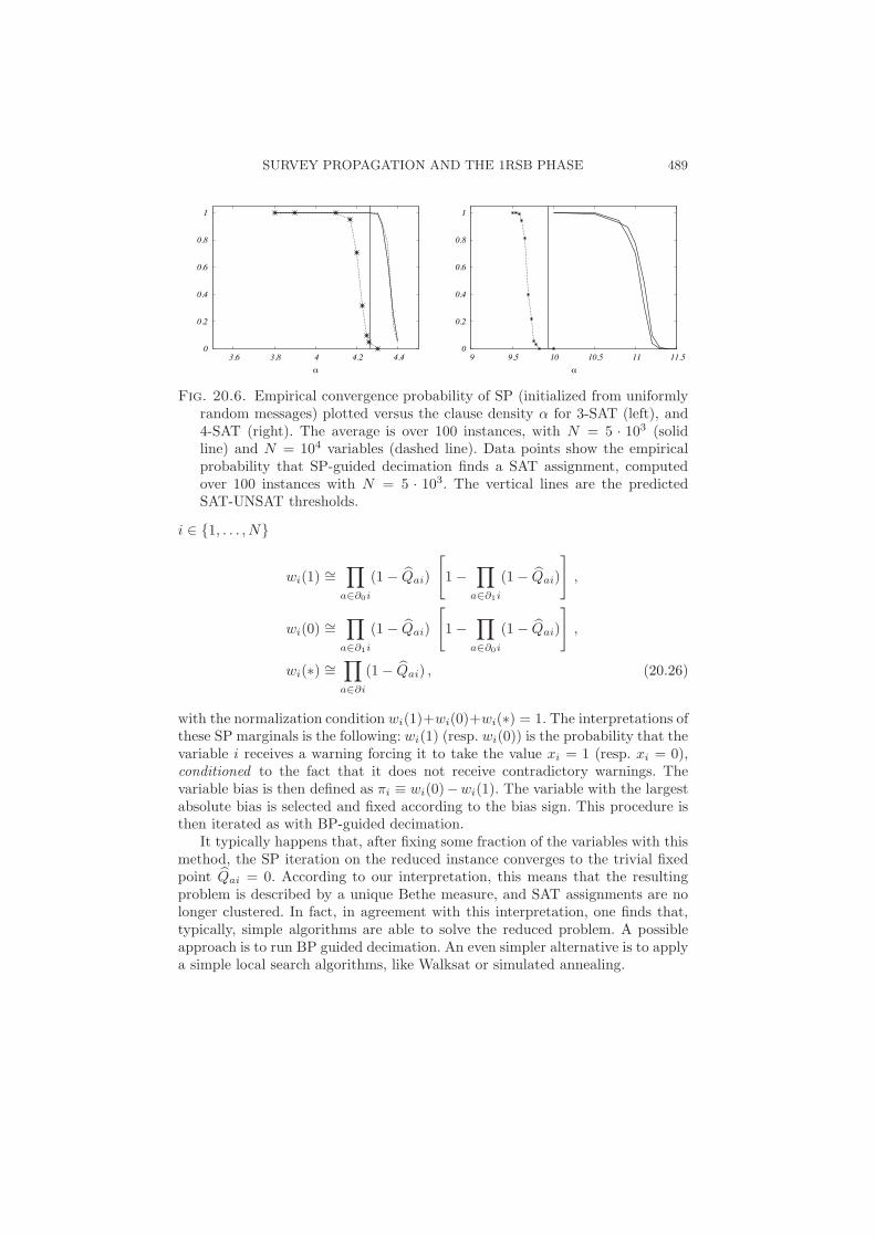
SURVEY PROPAGATION AND THE 1RSB PHASE 489
0
0.2
0.4
0.6
0.8
1
3.6 3.8 4 4.2 4.4α
0
0.2
0.4
0.6
0.8
1
9 9.5 10 10.5 11 11.5α
Fig. 20.6. Empirical convergence probability of SP (initialized from uniformlyrandom messages) plotted versus the clause density α for 3-SAT (left), and4-SAT (right). The average is over 100 instances, with N = 5 · 103 (solidline) and N = 104 variables (dashed line). Data points show the empiricalprobability that SP-guided decimation finds a SAT assignment, computedover 100 instances with N = 5 · 103. The vertical lines are the predictedSAT-UNSAT thresholds.
i ∈ 1, . . . , N
wi(1) ∼=∏
a∈∂0i
(1 − Qai)
[1 −
∏
a∈∂1i
(1 − Qai)
],
wi(0) ∼=∏
a∈∂1i
(1 − Qai)
[1 −
∏
a∈∂0i
(1 − Qai)
],
wi(∗) ∼=∏
a∈∂i
(1 − Qai) , (20.26)
with the normalization condition wi(1)+wi(0)+wi(∗) = 1. The interpretations ofthese SP marginals is the following: wi(1) (resp. wi(0)) is the probability that thevariable i receives a warning forcing it to take the value xi = 1 (resp. xi = 0),conditioned to the fact that it does not receive contradictory warnings. Thevariable bias is then defined as πi ≡ wi(0)−wi(1). The variable with the largestabsolute bias is selected and fixed according to the bias sign. This procedure isthen iterated as with BP-guided decimation.
It typically happens that, after fixing some fraction of the variables with thismethod, the SP iteration on the reduced instance converges to the trivial fixedpoint Qai = 0. According to our interpretation, this means that the resultingproblem is described by a unique Bethe measure, and SAT assignments are nolonger clustered. In fact, in agreement with this interpretation, one finds that,typically, simple algorithms are able to solve the reduced problem. A possibleapproach is to run BP guided decimation. An even simpler alternative is to applya simple local search algorithms, like Walksat or simulated annealing.

490 RANDOM K-SATISFIABILITY
The pseudocode for this algorithm is as follows.
SP-Guided Decimation (Formula F , SP parameter ε, tmax,WalkSAT parameters f , p)
1 : Set U = ∅;2 : Repeat until FAIL or U = V :3 : Call SP(F , ε, tmax). If it does not converge, FAIL;4 : For each i ∈ V \ U compute the bias πi;5 : Let j ∈ V \ U have the largest value of |πi|;6 : If |πj | ≤ 2Kε call WalkSAT(F , f, p);7 : Else fix xj according to the sign of πj ,
and define F as the new formula obtained after fixing xj ;8 : End-Repeat;9 : Return the current assignment;
SP (Formula F , Accuracy ε, Iterations tmax )1 : Initialize SP messages to i.i.d. random variables;2 : For t ∈ 0, . . . , tmax3 : For each (i, a) ∈ E
4 : Compute the new value of Qai using Eq. (20.10)5 : For each (i, a) ∈ E6 : Compute the new value of Qai using Eqs. (20.11-20.13)7 : Let ∆ be the maximum difference with previous iteration;8 : If ∆ < ε return current messages;9 : End-For;10 : Return ‘Not Converged’;
The WalkSAT pseudocode was given in Sec. 10.2.3.In Fig. 20.6 we plot the empirical success probability of SP-Guided Decima-
tion for random 3-SAT and 4-SAT formulae as a function of the clause densityα. A careful study suggests that the algorithm finds a satisfying assignment withhigh probability when α " 4.252 (for K = 3) and α " 9.6 (for K = 4). Thesevalues are slightly smaller than the conjectured locations of the SAT-UNSATthreshold αs(3) ≈ 4.2667 and αs(4) ≈ 9.931.
Apart from the SP routine (that builds upon the statistical mechanics in-sight) the above algorithm is quite naive and could be improved in a number ofdirections. One possibility is to allow the algorithm to backtrack, i.e. to releasesome variables that had been fixed at a previous stage of the decimation. Fur-ther, we did not use at any step the information provided by the free-entropyFe(y = ∞) that can be computed at little extra cost. Since this gives an estimateof the logarithm of the number solutions clusters, it can also be reasonable tomake choices that maximize the value of Fe in the resulting formula.

SURVEY PROPAGATION AND THE 1RSB PHASE 491
0
0.2
0.4
0.6
0.8
1
3.6 3.7 3.8 3.9 4 4.1 4.2 4.3 4.4α
0
0.2
0.4
0.6
0.8
1
9 9.2 9.4 9.6 9.8 10 10.2 10.4α
Fig. 20.7. Performance of BP-inspired decimation and SP-inspired decimationon 3-SAT (left plot) and 4-SAT (right plot) problems. Probability of findinga SAT assignment versus clause density, averaged over 100 instances withN = 5 · 103 variables. The SP based algorithm (dotted line) performs betterthan the BP based one (full line). The vertical lines are the SAT-UNSATthresholds.
As can be deduced from Fig. 20.7, SP-Guided Decimation outperforms BP-Guided Decimation. Empirically this algorithm, or small variations of it, providethe most efficient procedure for solving large random K-SAT formulae close tothe SAT-UNSAT threshold. Furthermore, it has extremely low complexity. EachSP iteration requires O(N) operations, which yields O(Ntmax) operations per SPcall. In the implementation outlined above this implies a O(N2tmax) complexity.This can however be reduced to O(Ntmax) by noticing that fixing a single variabledoes not affect the SP messages significantly. As a consequence, SP can be calledevery Nδ decimation steps for some small δ. Finally, the number of iterationsrequired for convergence seem to grow very slowly with N , if it does at all. Oneshould probably think of tmax as a big constant or tmax = O(log N)
In order to get a better understanding of how SP-guided decimation works, itis useful to monitor the evolution of the energetic complexity curve Σe(ε) whiledecimating. When SP iteration has converged on a given instance, one can use(20.21) to compute the free-entropy, and by a Legendre transform the curveΣe(ε).
In Fig. 20.8 we consider a run of SP-Guided Decimation on one random 3-SAT formula with N = 104 at α = 4.2. the complexity curve of the residualformula (NΣe(ε) versus the number of violated clauses Nε) is plotted every 1000decimation steps. One notices two main effects: (1) The zero-energy complexityNΣe(0) decreases, showing that some clusters of solutions are lost along thedecimation; (2) The number of violated clauses in the most numerous metastableclusters, the so-called ‘threshold energy’, decreases as well31, implying that the
31Because of the instability of the 1RSB solution at large energies (see Chapter 22), thethreshold energies obtained within the 1RSB approach are not exact. However one expects theactual behavior to be quantitatively close to the 1RSB description.

492 RANDOM K-SATISFIABILITY
0
0.005
0.01
0.015
0.02
0 0.0005 0.001 0.0015 0.002 0.0025 0.003 0.0035 0.004
Σ
ε
0
0.005
0.01
0.015
0.02
0.025
0 0.02 0.04 0.06 0.08 0.1 0.12 0.14
ε
Σe(ε)
Fig. 20.8. Decimation process: The complexity versus energy density (1/Ntimes the number of violated clauses) measured on a single instance of ran-dom 3-SAT with N = 10000 and α = 4.2 (top curve), and on the decimatedinstances obtained after fixing 1000, 2000, 3000 variables with the survey in-spired decimation procedure (from top to bottom). For comparison, the insetshows the same complexity versus total energy after fixing to arbitrary values1000, 2000, 3000 randomly chosen variables
problem becomes simpler: the true solutions are less and less hidden amongmetastable minima.
The important point is that the effect (2) is much more pronounced than(1). After fixing about half of the variables, the threshold energy vanishes. SPconverges to the trivial fixed point, the resulting instance becomes ‘simple,’ andis solved easily by Walksat.
20.3 Some ideas on the full phase diagram
20.3.1 Entropy of clusters
The energetic 1RSB cavity method has given two important results: on onehand, a method to locate the SAT-UNSAT transition threshold αs, which isconjectured to be exact, on the other, a powerful message passing algorithm: SP.These results were obtained at a cost: we completely forgot about the size of theclusters of SAT assignments, their ‘internal entropy’.
In order to get a finer understanding of geometry of the set of solutions inthe SAT phase, we need to get back to the uniform measure over SAT assign-ments of (20.1), and use the 1RSB method of Sec. 19.2. Our task is in principlestraightforward: we need to estimate the 1RSB free entropy F(x), and performthe Legendre transform (19.8) in order to get the complexity function Σ(φ).Recall that Σ(φ) is the exponential growth rate of the number of clusters withfree-entropy Nφ (in the present case, since we restrict to SAT configurations,the free-entropy of a cluster is equal to its entropy).

SOME IDEAS ON THE FULL PHASE DIAGRAM 493
-0.02
-0.01
0
0.01
0.02
0.03
0.04
0 0.01 0.02 0.03 0.04 0.05 0.06 0.07 0.08 0.09
-0.02
0
0.02
0.04
0.06
0.08
8 8.5 9 9.5 10 10.5
φ
Σ(φ)
α
Σ(x = 0)
Σ(x = 1)
αd
αc
αs
fRS
F(x = 1)
F(x = 0) F(x∗)
Fig. 20.9. 1RSB analysis of random 4-SAT. Left: Complexity versus internalentropy density of clusters, for α = 9.3, 9.45, 9.6, 9.7, 9.8, 9.9 (from top tobottom). When sampling uniformly SAT configurations, one finds either con-figurations in an exponentially large number of clusters (dot on the curveα = 9.45, which is the point where dΣ/dφ = −1), or a condensed phasewhere the measure is dominated by a few clusters (squares on the curveswith α ≥ 9.6). Right: Complexity Σ(x) and free-entropy density F(x) at afew key values of x: x = 0 corresponds to the maximum of Σ(φ), x = 1 tothe point with dΣ/dφ = −1, and x = x∗ to Σ(φ) = 0. The dynamical tran-sition is at αd ≈ 9.38, the condensation transition at αc ≈ 9.547, and theSAT-UNSAT transition at αs ≈ 9.931.
This is a rather demanding task from the numerical point of view. Let us un-derstand why: each BP message is parameterized by one real number in [0, 1], aswe saw in (20.3). A 1RSB message characterizes the distribution of this number,so it is a pdf on [0, 1]. One such distribution is associated to each directed edgeof the factor graph. For the study of the phase diagram, one needs to performa statistical analysis of the 1RSB messages. Within the population dynamicsapproach this means that we must use a (large) population of distribution func-tions. For each value of x, the algorithm must be run for a large enough numberof iterations to estimate F(x). This is at the limit of what can be done numeri-cally. Fortunately it can be complemented by two simpler computations: the SPapproach which gives the results corresponding to x = 0, and the study of thex = 1 case using the simplification described in Sec. 19.4.
20.3.2 The condensation transition for K ≥ 4
We shall not provide any technical detail of these computations, but focus onthe main results using K = 4-SAT as a running example. As shown by Fig. 20.9,this system displays the full scenario of phase transitions explained in Sec. 19.6.Upon increasing the clause density α, one finds first a RS phase for α < αd, thena d1RSB phase with exponentially many relevant states for αd < α < αc, then as1RSB phase with condensation of the measure on a few states, for αc < α < αs.The system becomes UNSAT for α > αs.
Fig. 20.9 shows the evolution of the complexity versus internal entropy density

494 RANDOM K-SATISFIABILITY
of the clusters when α increases (note that increasing α plays the same role asdecreasing the temperature in the general scenario sketched in Fig. 19.6). For agiven α, almost all clusters have an internal entropy density φ0 corresponding tothe maximum of Σ(φ). The complexity at the maximum, Σ(φ0) = F(x = 0), isequal to the complexity at zero energy density that we found with the energetic1RSB cavity method. When sampling SAT configurations uniformly, almost allof them are found in clusters of internal entropy density φ1 such that Σ(φ) + φis maximum, conditioned to the fact that Σ(φ) ≥ 0. In the d1RSB phase onehas Σ(φ1) > 0, in the s1RSB one has Σ(φ1) = 0. The condensation point αc cantherefore be found through a direct (and more precise) study at x = 1. Indeed itis identified as the value of clause density such that the two equations: Σ(φ) = 0,dΣ/dφ = −1 admit a solution.
Exercise 20.8 Using the Legendre transform 19.8, show that this condensa-tion point αc is the one where the 1RSB free-entropy function F(x) satisfiesF(1) − F′(1) = 0 (where ′ means derivative with respect to x). As we saw inSec. 19.4, the value of F(1) is equal to the RS free-entropy. As for the valueof the internal entropy F′(1), it can also be obtained explicitly from the x = 1formalism. Writing down the full x = 1 formalism for random satisfiability,including this computation of F′(1), is an interesting (non-trivial) exercise.
The dynamical transition point αd is defined as the smallest value of α suchthat there exists a non-trivial solution to the 1RSB equation at x = 1 (in practiceit is best studied using the point-to-set correlation which will be described inCh. 22). Notice from Fig. 20.9 that there can exist clusters of SAT assignmentseven at α < αd: for α = 4.3, there exists a branch of Σ(φ), around the point φ0
where it is maximum, but this branch disappears, if one increases φ, before onecan find a point where dΣ/dφ = −1. The interpretation of this regime is thatan exponentially small fraction of the solutions are grouped in well separatedclusters. The vast majority of the solutions belongs instead to a single, wellconnected ‘replica symmetric’ cluster. As we saw in the energetic cavity method,the first occurrence of the clusters around φ0 occurs at the value αd,SP which isaround 8.3 for 4-SAT.
The same scenario has been found in the studies of random K-SAT withK = 5, 6, and it is expected to hold for all K ≥ 4. The situation is somewhatdifferent at K = 3, as the condensation point αc coincides with αd: the 1RSBphase is always condensed. Table 20.3.2 summarizes the values of the thresholds.
20.4 An exercise: coloring random graphs
Recall that a proper q-coloring of a graph G = (V , E) is an assignment of colors1, . . . , q to the vertices of q in such a way that no edge has the two adjacentvertices of the same color. Hereafter we shall refer to a proper q-coloring asto a ‘coloring’ of G. Colorings of a random graph can be studied following theapproach just described for satisfiability, and reveal a strikingly similar behavior.

AN EXERCISE: COLORING RANDOM GRAPHS 495
K αd αc αs
3 3.86 3.86 4.26674 9.38 9.547 9.9315 19.16 20.80 21.1176 36.53 43.08 43.37
Table 20.2 Predictions of the 1RSB cavity method for the non-trivial SP, dy-namical, condensation, and SAT-UNSAT threshold of random K-satisfiability
Here we shall just present some key steps of this analysis: this section can beseen as a long exercise in applying the cavity method. We shall focus on thecase of random regular graphs, which is technically simpler. In particular, manyresults can be derived without resorting to a numerical resolution of the cavityequations. The reader is encouraged to work out the many details which are leftaside.
We shall adopt the following description of the problem: to each vertex i ∈ Vof a graph G = (V , E), associate a variable xi ∈ 1, · · · , q. The energy of a colorassignment x = x1, · · · , xN is given by the number of edges whose verticeshave the same color:
E(x) =∑
(ij)∈E
I(xi = xj) . (20.27)
If the graph is colorable, one is also interested in the uniform measure over propercolorings:
µ(x) =1
ZI(E(x) = 0) =
1
Z
∏
(ij)∈E
I(xi .= xj) , (20.28)
where Z is the number of proper colorings of G. The factor graph associatedwith µ( · ) is easily constructed. Associate one variable node to each vertex ofi ∈ G, one function node to each edge (ij) ∈ C, and connect this function it tothe variable nodes corresponding to i and j. The probability distribution µ(x) istherefore a pairwise graphical model.
We will assume that G is a random regular graphs of degree c. Equivalently,the corresponding factor graph is distributed according to the DN (Λ, P ) ensem-ble, with Λ(x) = xc and P (x) = x2. The important technical simplification isthat, for any fixed r, the radius-r neighborhood around a random a vertex i iswith high probability a tree of degree c, i.e. it is non-random. In other words,the neighborhood of most of the nodes is the same.
Let us start with the RS analysis of the graphical model (20.28). As we sawin Sec. 14.2.5, we can get rid of function-to-variable node messages, and workwith variable-to-function messages νi→j(xi). The BP equations read
νi→j(x) ∼=∏
k∈∂i\j
(1 − νk→i(x)) . (20.29)
496 RANDOM K-SATISFIABILITY
Because of the graph regularity, there exists solutions of these equations such thatmessages take the same value on all edges. In particular, Eq. (20.29) admits thesolution νi→j( · ) = νunif( · ), where νunif( · ) is the uniform messages: νunif(x) =1/q for x ∈ 1, . . . , q. The corresponding free-entropy density (equal here to theentropy density) is
fRS = log q +c
2log
(1 − 1
q
). (20.30)
It can be shown that this coincides with the ‘annealed’ estimate N−1 log EZ. Itdecreases with the degree c of the graph and becomes negative for c larger thancUB(q) ≡ 2 log q/ log(q/(q − 1)), similarly to what we saw in Fig. 20.2. Markovinequality implies that, with high probability, a random c-regular graph doesnot admit a proper q-coloring for c > cUB(q). Further, the RS solution is surelyincorrect for c > cUB(q).
The stability analysis of this solution shows that the spin glass susceptibilitydiverges as c ↑ cst(q), with cst(q) = q2 − 2q + 2. For q ≥ 4, cst(q) > cUB(q).
In order to correct the above inconsistencies, one has to resort to the energetic1RSB approach. Let us focus onto y →∞ limit (equivalently, on the zero energylimit). In this limit one obtains the SPequations. This can be written in termsof messages Qi→j( · ) that have the following interpretation
Qi→j(x) = probability that, in absence of (i, j), xi is forced to value x,
Qi→j(∗) = probability that, in absence of (i, j), xi is not forced.
Recall that ‘probability’ is interpreted here with respect to a random Bethe state.An SP equation express the message Qi→j( · ) in terms of the c− 1 incoming
messages Qk→i( · ) with k ∈ ∂i \ j. To keep notations simple, we fix an edgei → j and denote it by 0, while we use 1 . . . , c− 1 to label the edges k → i withk ∈ ∂i \ j. Then, for any x in 1, · · · , q, one has:
Q0(x) =
∑(x1...xc−1)∈N (x) Q1(r1)Q2(x2) · · ·Qc−1(xc−1)∑
(x1...xc−1)∈D Q1(r1)Q2(x2) · · ·Qc−1(xc−1). (20.31)
where:
• D is the set of tuples (x1, · · · , xc−1) ∈ ∗, 1, · · · , qn such that there ex-ist z ∈ 1, · · · , q with z .= x1, . . . , xc−1. According to the interpretationabove, this means that there is no contradiction among the warmings to i.
• N (x) is the set of tuples (x1, · · · , xc−1) ∈ D such that, for any z .= x thereexists k ∈ 1, . . . , c − 1 such that xk = z. In other words, x is the onlycolor for vertex i that is compatible with the warnings.
Q0(∗) is determined by the normalization condition Q0(∗) +∑
x Q0(x) = 1.On a random regular graph of degree c, these equations admit a solution
with Qi→j( · ) = Q( · ) independent of the edge (i, j). Furthermore, if we assume

AN EXERCISE: COLORING RANDOM GRAPHS 497
q cd,SP cd cc cs
3 5 5 6 64 9 9 10 105 13 14 14 156 17 18 19 2010 36 39 43 44
-0.05
0
0.05
0.1
0.15
0 0.02 0.04 0.06 0.08 0.1 0.12 0.14φ
Σ(φ)
c = 17
c = 18
c = 19
c = 20
Fig. 20.10. Results of the 1RSB analysis of proper q-colorings of random regulargraphs. The table gives the thresholds: appearance of non-trivial SP solutionscd,SP, dynamical cd, condensation cc, colorable/uncolorable cs. The figureshows the clusters complexity as a function of their internal entropy density.Here q = 6 and the graph degrees are c = 17 (RS), c = 18 (d1RSB), c = 19(s1RSB) and c = 20 (uncolorable). The circles denote the points of slope −1on the complexity curves.
this solution to be symmetric under permutation of colors, the correspondingmessage can by parameterized by a single number a ∈ [0, 1/q]:
Q(x) = a for x ∈ 1, · · · , q ,
Q(∗) = 1 − qa . (20.32)
Plugging this Ansatz in Eq. (20.31), we get:
a =
∑q−1r=0 (−1)r
(q−1
r
)(1 − (r + 1)a)c−1
∑q−1r=0 (−1)r
( qr+1
)(1 − (r + 1)a)c−1
. (20.33)
The complexity Σe(ε = 0) yielding the exponential growth rate of the number ofclusters of proper colorings, is given by Σe(e = 0) = limy→∞ Fe(y). One finds:
Σe(ε = 0; c, q) = log
(q−1∑
r=0
(−1)r
(q
r + 1
)(1 − (r + 1)a)c
)− c
2log(1 − qa2) .
(20.34)
Given the number of colors q, one can study what happens when the degree cgrows (which amounts to increasing the density of constraints). The situation isvery similar to the one found in satisfiability. For c ≥ cd,SP(q), there exists a pairof non-trivial solution to Eq.(20.33) with a > 0. The complexity Σe(e = 0) canbe computed from (20.34) (evaluated on the largest solution a of Eq. (20.33)),
498 RANDOM K-SATISFIABILITY
and is decrasing in c. It becomes negative for c ≥ cs(q). The degree cs(q) is thusthe 1RSB prediction for the SAT-UNSAT threshold.
When c < cs(q), the uniform measure over valid colorings can be studied,and in particular one can characterize the distribution of entropy of clusters.Fig. 20.10 shows the complexity as function of internal entropy density of clusters.The similarity to Fig. 20.9 is obvious. One can define two particularly relevantthresholds: cd is the smallest degree such that the 1RSB equations at x = 1have a non-trivial solution, and cc is the smallest degree such that the uniformmeasure over proper colorings is ‘condensed’. The table in Fig. 20.10 gives someexamples of these thresholds. An asymptotic analysis for large q shows that:
cd,SP = q(log q + log log q + 1 − log 2 + o(1)) (20.35)
cd = q(log q + log log q + O(1)) (20.36)
cc = 2q log q − log q − 2 log 2 + o(1) (20.37)
cs = 2q log q − log q − 1 + o(1) (20.38)
These predictions can be rephrased into a statement on the chromatic num-ber, i.e. the minimal number of colors needed to color a graph. Because of theheuristic nature of the approach, we formulate it as a conjecture:
Conjecture 20.1 With high probability, the chromatic number of a random reg-ular graph with N vertices and degree c ≥ 4 is equal to χchrom(c), where
χchrom(c) = maxq : Σe(ε = 0; c, q) > 0 . (20.39)
Here Σe(ε = 0; c, q) is given by Eq. (20.34) with a the largest solution of (20.33)in the interval [0, 1/q].
Using the numbers in table 20.10, this conjecture predicts for instance thatχchrom(c) = 3 for c = 4, 5, χchrom(c) = 4 for c = 6, 7, 8, 9, and χchrom(c) = 5for 10 ≤ c ≤ 14.
On the side of rigorous results, a clever use of the first and second momentmethods allows to prove the following result:
Theorem 20.2 With high probability, the chromatic number of a random regulargraph with N vertices and degree c is either k or k + 1 or k + 2, where k is thesmallest integer such that c < 2k log k. Furthermore, if c > (2k − 1) log k, thenwith high probability the chromatic number is either k or k + 1.
One can check explicitely that the results of the 1RSB cavity conjecture agreewith this theorem, that proves the correct leading behavior at large c.
While this presentation was focused on random regular graphs, a large classof random graph ensembles can be analyzed along the same lines.
Notes
Random K-satisfiability was first analyzed using the replica symmetric cavitymethod in (Monasson and Zecchina, 1996; Monasson and Zecchina, 1996). The

NOTES 499
resulting equations are equivalent to a density evolution analysis of belief propa-gation. BP was used as an algorithm for finding SAT assignments in (Pumphrey,2001). This study concluded that BP is ineffective in solving satisfiability prob-lems, mainly because it assigned variables in a one-shot fashion, unlike in deci-mation.
The 1RSB cavity method was applied to random satisfiability in (Mezard,Parisi and Zecchina, 2003; Mezard and Zecchina, 2002), where the value of αc wascomputed for 3-SAT. This approach was applied to larger K in (Mertens, Mezardand Zecchina, 2006), which also derived the large K asymptotics. The SPY andSP equations for satisfiability were first written in (Mezard and Zecchina, 2002),where SP-inspired decimation was introduced (Fig. 20.8 is borrowed from thispaper). A more algorithmic presentation of SP was then developed in (Braun-stein, Mezard and Zecchina, 2005), together with an optimized source code forSP and decimation (Braunstein, Mezard and Zecchina, 2004). The idea of back-tracking was suggested in (Parisi, 2003), but its performances have not beensystematically studied yet.
The condensation phenomenon was discussed in (Krzakala, Montanari, Ricci-Tersenghi, Semerjian and Zdeborova, 2007), in relation with studies of the en-tropic complexity in colouring (Mezard, Palassini and Rivoire, 2005b; Krzakalaand Zdeborova, 2007) and in satisfiability (Montanari, Ricci-Tersenghi and Se-merjian, 2008).
The analysis in this chapter is heuristic, and is waiting for a rigorous proof.Let us point out that one important aspect of the whole scenario has been estab-lished rigorously for K ≥ 8: it has been shown that in some range of clause densitybelow αs(K), the SAT assignments are grouped into exponentially many clusters,well separated from each other (Mezard, Mora and Zecchina, 2005a; Achlioptasand Ricci-Tersenghi, 2006; Daude, Mezard, Mora and Zecchina, 2008). This re-sult can be obtained by a study of ‘x-satisfiability’ problem, that requires todetermine whether a formula has two SAT assignments differing in xN vari-ables. Bounds on the x-satisfiability threshold can be obtained through the firstand second moment methods.
The coloring problem has been first studied with the energetic 1RSB cav-ity method by (Mulet, Pagnani, Weigt and Zecchina, 2002; Braunstein, Mulet,Pagnani, Weigt and Zecchina, 2003): these papers contain the derivation of theSAT/UNSAT threshold and the SP equations. A detailed study of the entropy ofclusters, and the computation of the other thresholds, has carried out in (Krza-kala and Zdeborova, 2007). These papers also study the case of Erdos Renyigraphs. Theorem 20.2 was proven in (Achlioptas and Moore, 2004), and its ana-logue for Erdos Renyi graphs in (Achlioptas and Naor, 2005).

21
GLASSY STATES IN CODING THEORY
In Ch. 15 we studied the problem of decoding random LDPC codes, and foundtwo phase transitions, that characterize the code performances in the large block-length limit. Consider, for instance, communication over a binary symmetricchannel with crossover probability p. Under belief propagation decoding, the biterror rate vanishes in the large blocklength limit below a first threshold pd andremains strictly positive for p > pd. On the other hand, the minimal bit errorrate achievable with the same ensemble (i.e. the bit error rate under symbolMAP decoding) vanishes up to a larger noise level pc and is bounded away from0 for p > pc.
In principle, one should expect each decoding algorithm to have a differentthreshold. This suggests not to attach too much importance to the BP thresholdpd. On the contrary, we will see in this chapter that pd is, in some sense, a‘universal’ characteristics of the code ensemble: above pd, the decoding problemis plagued by an exponential number of metastable states (Bethe measures). Inother words the phase transition which takes place at pd is not only algorithmic,it is a structural phase transition. This transition turns out to be a dynamical1RSB glass transition and this suggests that pd is the largest possible thresholdfor a large class of local decoding algorithms.
We have already seen in the last section of Ch. 15 that the two thresholdspd and pc are closely related and can both be computed formally within the RScavity method, i.e. in terms of the density evolution fixed point. The analysisbelow will provide a detailed explanation of this connection in terms of the glasstransition studied in Ch.19.
In the next section we start by a numerical investigation of the role ofmetastable states in decoding. Sec. 21.2 considers the particularly instructivecase of the binary erasure channel, where the glassy states can be analyzed rel-atively easily using the energetic 1RSB cavity method. The analysis of generalmemoryless channels is described in Sec. 21.3. Finally, Sec. 21.4 draws the con-nection between metastable states, which are a main object of study in thischapter, and trapping sets (subgraphs of the original factor graph that are oftenregarded as responsible for coding failures).
21.1 Local search algorithms and metastable states
The codewords of an LDPC code are solutions of a constraint satisfaction prob-lem. The variables are the bits of a word x = (x1, x2, . . . , xN ), with xi ∈ 0, 1,and the constraints are the parity check equations, i.e. a set of linear equations
500

LOCAL SEARCH ALGORITHMS AND METASTABLE STATES 501
mod 2. This is analogous to the XORSAT problem considered in Ch. 18, althoughthe ensembles of linear systems used in coding are different.
An important difference with XORSAT is that we are looking for a specificsolution of the linear system, namely the transmitted codeword. The receivedmessage y gives us a hint of where to look for this solution. For notationalsimplicity, we shall assume that the output alphabet Y is discrete, and the chan-nel is a binary input memoryless output symmetric (BMS- see Ch. 15) channelwith transition probability32 Q(y|x). The probability that x is the transmittedcodeword, given the received message y, is given by the usual formula (15.1)P(x|y) = µy(x) where:
µy(x) ∼=N∏
i=1
Q(yi|xi)M∏
a=1
I(xia1⊕ · · ·⊕ xia
k(a)= 0) . (21.1)
It is natural to associate an optimization problem to the code. Define theenergy E(x) of a word x (also called a ‘configuration’) as twice the number ofparity check equations violated by x (the factor 2 is introduced for future simpli-fications). Codewords coincide with the global minima of this energy function,with zero energy.
We already know that decoding consist in computing marginals of the distri-bution µy(x) (symbol MAP decoding), or finding its argmax (word MAP decod-ing). In the following we shall discuss two closely related problems: (i) optimizingthe energy function E(x) within a subset of the configuration space defined bythe received word and the channel properties; (ii) sampling from a ‘tilted’ Boltz-mann distribution associated to E(x).
21.1.1 Decoding through constrained optimization
Let us start by considering the word-MAP decoding problem. We shall ex-ploit our knowledge of the BMS channel. Conditional on the received wordy = (y1, y2, . . . , yN), the log-likelihood for x to be the channel input is:
Ly(x) =N∑
i=1
logQ(yi|xi) . (21.2)
We shall later use the knowledge that the input word was a codeword, but Ly(x)
is well defined for any x ∈ 0, 1N , regardless of whether it is a codeword or not,so let us first characterize its properties.
Assume without loss of generality that the codeword 0 had been transmitted.By the law of large numbers, for large N the log-likelihood of this codeword isclose to −Nh, where h is the channel entropy: h = −
∑y Q(y|0) logQ(y|0). The
probability of an order-N deviation away from this value is exponentially small
32Throughout this chapter we adopt a different notation for the channel transition probabilitythan in the rest of the book, in order to avoid confusion with 1RSB messages.
502 GLASSY STATES IN CODING THEORY
in N . This suggests to look for the transmitted codeword among those x suchthat Ly(x) is close to h.
The corresponding ‘typical pairs’ decoding strategy goes as follows: Giventhe channel output y, look for a codeword x ∈ C, such that Ly(x) ≥ −N(h + δ).We shall refer to this condition as the ‘distance constraint’. For instance, inthe case of the BSC channel, it amounts to constraining the Hamming distancebetween the codeword x and the received codeword y to be small enough. Ifexactly one codeword satisfies the distance constraint, return it. If there is nosuch codeword, or if there are several of them, declare an error. Here δ > 0 isa parameter of the algorithm, which should be thought of as going to 0 afterN →∞.
Exercise 21.1 Show that the block error probability of typical pairs decodingis independent of the transmitted codeword.[Hint: use the linear structure of LDPC codes, and the symmetry property ofthe BMS channel.]
Exercise 21.2 This exercise aims at convincing the reader that typical pairsdecoding is ‘essentially’ equivalent to maximum likelihood (ML) decoding.
(a) Show that the probability that no codeword exists with Ly(x) ∈ [−N(h+δ),−N(h− δ)] is exponentially small in N .[Hint: apply Sanov Theorem, cf. Sec. 4.2, to the type of the receivedcodeword.]
(b) Upper bound the probability that ML succeeds and typical pairs decodingfails in terms of the probability that there exists an incorrect codeword xwith Ly(x) ≥ −N(h+ δ), but no incorrect codeword Ly(x) ≥ −N(h− δ).
(c) Estimate the last probability for Shannon’s random code ensemble. Showin particular that it is exponentially small for all noise levels strictlysmaller than the MAP threshold and δ small enough.
Since codewords are global minima of the energy function E(x) we canrephrase typical pairs decoding as an optimization problem:
Minimize E(x) subject to Ly(x) ≥ −N(h + δ) . (21.3)
Neglecting exponentially rare events, we know that there always exists at leastone solution with cost E(x) = 0, corresponding to the transmitted codeword.Therefore, typical pairs decoding is successful if and only if the minimum is non-degenerate. This happens with high probability for p < pc. On the contrary,for p > pc, the optimization admits other minima with zero cost (incorrectcodewords). We already explored this phenomenon in chapters 11 and 15, andwe shall discuss it further below. For p > pc there exists an exponential number ofcodewords whose likelihood is larger or equal to the likelihood of the transmittedone.

LOCAL SEARCH ALGORITHMS AND METASTABLE STATES 503
Similarly to what we have seen in other optimization problems (such as MAX-XORSAT or MAX-SAT), generically there exists an intermediate regime pd <p < pc, which is characterized by an exponentially large number of metastablestates. For these values of p, the global minimum of E(x) is still the transmittedcodeword, but is ‘hidden’ by the proliferation of deep local minima. Remarkably,the threshold for the appearence of an exponential number of metastable statescoincides with the BP threshold pd. Thus, for p ∈]pd, pc[ MAP decoding wouldbe successful, but message passing decoding fails. In fact no practical algorithmwhich succeeds in this regime is known. A cartoon of this geometrical picture ispresented in Fig. 21.1.
At this point, the reader might be puzzled by the observation that findingconfigurations with E(x) = 0 is per se a polynomial task. Indeed it amountsto solving a linear system modulo 2, and can be done by Gauss elimination.However, the problem (21.3) involves the condition Ly(x) ≥ −N(h + δ) which isnot a linear constraint modulo 2. If one resorts to local-search based decodingalgorithms, the proliferation of metastable states for p > pd can block the algo-rithms. We shall discuss this phenomenon on two local search strategies: ∆-localsearch and simulated annealing.
21.1.2 ∆ local-search decoding
A simple local search algorithm consists in starting from a word x(0) such thatLy(x(0)) ≥ −N(h + δ) and then recursively constructing x(t + 1) by optimizingthe energy function within a radius ∆ neighborhood around x(t):
∆ local search (channel output y, search size ∆, likelihood resolution δ)1: Find x(0) such that Ly(x(0)) ≥ −N(h + δ) ;2: for t = 0, . . . tmax − 1:3: Choose a uniformly random connected set U ⊂ 1, . . . , N
of variable nodes in the factor graph with |U | = ∆;4: Find the configuration x′ that minimizes the energy subject
to x′j = xj for all j .∈ U ;
5: If Ly(x′) ≥ −N(h + δ), set x(t + 1) = x′;otherwise, set x(t + 1) = x(t);
6: end;7: return x(tmax).
(Recall that a set of variable nodes U is ‘connected’ if, for any i, j ∈ U , thereexists a path in the factor graph connecting i to j, such that all variable nodesalong the path are in U as well.)
Exercise 21.3 A possible implementation of step 1 consists in setting xi(0) =argmaxx Q(yi|x). Show that this choice meets the likelihood constraint.

504 GLASSY STATES IN CODING THEORY
Fig. 21.1. Three possible cartoon landscapes for the energy function E(x) (thenumber of violated checks), plotted in the space of all configurations x withLy(x) ≥ N(h − δ). On the left: the energy as a unique global minimumwith E(x) = 0 (the transmitted codeword) and no (deep) local minima. Cen-ter: many deep local minima appear although the global minimum remainsnon-degenerate. Right: More than one codeword is compatible with the like-lihood constraint, and the global minimum E(x) = 0 becomes degenerate.
If the factor graph has bounded degree (which is the case with LDPC en-sembles), and ∆ is bounded as well, each execution of the cycle above impliesa bounded number of operations. As a consequence if we let tmax = O(N), thealgorithm has linear complexity. A computationally heavier variant consists inchoosing U at step 3 greedily. This means going over all such subsets and thentaking the one that maximizes the decrease in energy |E(x(t + 1))− E(x(t))|.
Obviously the energy E(x(t)) of the configuration produced after t iterationsis a non-increasing function of t. If it vanishes at some time t ≤ tmax, then thealgorithm implements a typical pairs decoder. Ideally, one would like a charac-terization of the noise levels and code ensembles such that E(x(tmax)) = 0 withhigh probability.
The case ∆ = 1 was analyzed in Ch. 11, under the name of ‘bit-flipping’algorithm, for communicating over the channel BSC(p). We saw that there existsa threshold noise level p1 such that, if p < p1 the algorithm returns with highprobability the transmitted codeword. It is reasonable to think that the algorithmwill be unsuccessful with high probability for p > p1.
Analogously, one can define thresholds p∆ for each value of ∆. Determiningthese thresholds analytically is an extremely challenging problem.
One line of approach could consist in first studying ∆-stable configura-tions. We say that a configuration x is ∆-stable if, for any configuration x′ suchthat Ly(x′) ≥ −N(h + δ) and d(x, x′) ≤ ∆, E(x′) ≥ E(x).
Exercise 21.4 Show that, if no ∆-stable configurations exists, then the greedyversion of the algorithm will find a codeword after at most M steps (M beingthe number or parity checks).
While this exercise hints at a connection between the energy landscape andthe difficulty of decoding, one should be aware that the problem of determiningp∆ cannot be reduced to determining whether ∆-stable states exist or to estimate

LOCAL SEARCH ALGORITHMS AND METASTABLE STATES 505
their number. The algorithm indeed fails if, after a number t of iterations, thedistribution of x(t) is (mostly) supported in the basin of attraction of ∆-stablestates. The key difficulty is of course to characterize the distribution of x(t).
21.1.3 Decoding through simulated annealing
A more detailed understanding of the role of metastable configurations in thedecoding problem can be obtained through the analysis of the MCMC decodingprocedure that we discussed in Sec. 13.2.1. We thus soften the parity checkconstraints through the introduction of an inverse temperature β = 1/T (thisshould not be confused with the temperature introduced in Ch. 6, which insteadmultiplied the codewords log-likelihood). Given the received word y, we definethe following distribution over the transmitted message x, cf. Eq. (13.10):
µy,β(x) ≡ 1
Z(β)exp−βE(x)
N∏
i=1
Q(yi|xi) . (21.4)
This is the ‘tilted Boltzmann form’ that we alluded to before. In the low-temperature limit it reduces to the familiar a posteriori distribution which wewould like to sample: µy,β=∞(x) is supported on the codewords, and gives to eachof them a weight proportional to its likelihood. At infinite temperature, β = 0,the distribution factorizes over the bits xi. More precisely, under µy,β=0(x), thebits xi are independent random variables with marginal Q(yi|xi)/(Q(yi|0) +Q(yi|1)). Sampling from this measure is very easy.
For β ∈]0,∞[, µy,β( · ) can be regarded as a distribution of possible channelinputs for a code with ‘soft’ parity check constraints. Notice that, unlike theβ = ∞ case, it depends in general on the actual parity check matrix and notjust on the codebook C. This is actually a good feature of the tilted measure:performances of practical algorithms do indeed depend upon the parity checkmatrix representation of C. It is therefore necessary to take it into account.
We shall sample from µy,β( · ) using Glauber dynamics, cf. Sec. 13.2.1. Wehave already seen in that section that decoding through sampling at a fixed βfails above a certain noise level. Let us now try to improve on it using a simulatedannealing procedure in which β is increased gradually according to an annealingschedule β(t), with β(0) = 0. This decoder uses as input the received word y,the annealing schedule, and some maximal numbers of iterations tmax, n:
Simulated Annealing Decoder ( y, β(t), tmax, n )1: Generate x∗(0) form µy,0( · );2: for t = 0, . . . tmax − 1:3: Set x(0; t) = x∗(t− 1);4: Let x(j; t), j ∈ 1, . . . , n be the configurations produced by
n successive Glauber updates at β = β(t);5: Set x∗(t) = x(n; t);6: end7: return x(tmax).

506 GLASSY STATES IN CODING THEORY
0.00
0.05
0.10
0.15
0.20
0.25
0.30
0.0 0.2 0.4 0.6 0.8 1.0 1.2
τ =1τ =10τ =102
0.00
0.05
0.10
0.15
0.20
0.25
0.30
0.0 0.2 0.4 0.6 0.8 1.0 1.2
τ =10τ =102
τ =103
T T
eann eann
Fig. 21.2. Decoding random codes from the (5, 6) LDPC ensemble through sim-ulated annealing. Here we consider blocklength N = 12000 and transmissionover the BSC(p) with p = 0.12 (left) and 0.25 (right). The system is annealedthrough tmax = 1200 temperature values equally spaced between T = 1.2 andT = 0. At each temperature n = Nτ updates are executed. Statistical errorsare comparable with the size of jumps along the curves.
Its algorithmic complexity is proportional to the total number of Glauberupdates ntmax. If we want the algorithm to be efficient, this should grow linearlyor slightly super-linearly with N . The intuition is that the first (small β) stepsallow the Markov chain to equilibrate across the configuration space while, as βgets larger, the sample concentrates onto (or near to) codewords. Hopefully ateach stage x∗(t) will be approximately distributed according to µy,β(t)( · ).
Figure 21.2 shows the result obtained by the simulated annealing decoder,using random LDPC codes from the (5, 6) regular ensemble, used over the binarysymmetric channel at crossover probabilities p = 0.12 and 0.25 (for this ensemble,pd ≈ 0.139 and pc ≈ 0.264). The annealing schedule is linear in the temperature,namely β(t) = 1/T (t) with
T (t) = T (0)−T (0)− T (tmax)
( t
tmax
), (21.5)
with T (0) = 1.2 and T (tmax) = 0. The performance of decoding can be evaluatedthrough the number of violated checks in the final configuration, which is halfE(x(tmax)). The figure shows the energy density averaged over 10 repetitions ofthe decoding experiment (each time with a new code randomly chosen from theensemble), e(t) = 1
N 〈E(x(t))〉, versus the temperature T (t). As the number ofupdates performed at each temperature increases, the number of violated checksper variable seems to converge to a well defined limiting value, that depends ont only through the corresponding temperature
1
N〈E(x(t))〉 → eann(β(t)) . (21.6)
Further, E(x(t))/N seems to concentrate around its mean as N →∞.

LOCAL SEARCH ALGORITHMS AND METASTABLE STATES 507
At small p, the curve eann(β) quickly converges to 0 as β → ∞: a codeword(the transmitted one) is found efficiently. In fact, already at β = 1, the numericalresult for eann(β) is indistinguishable from 0. We expect that eann(β) coincideswithin numerical accuracy with the theoretical prediction for the equilibriumaverage
eeq(β) ≡ 1
Nlim
N→∞〈E(x)〉β . (21.7)
This agrees with the above observations since eeq(β) = O(e−10β) (the lowestexcitation over the ground state amounts to flipping a single bit, its energy isequal to 10). The numerics thus suggest that x(tmax) is indeed approximatelydistributed according to µy,β(t)( · ).
At large p, eann(β) has instead a non-vanishing β → ∞ limit: the annealingalgorithm does not find any codeword. The returned word x∗(tmax) typicallyviolates Θ(N) parity checks. On the other hand, in the equilibrated system at β =∞, the energy vanishes by construction (we know that the transmitted codewordsatisfies all checks). Therefore the simulation has fallen out of equilibrium atsome finite β, thus yielding a distribution of x(tmax) which is very different fromµy,β=∞( · ). The data in Fig. 21.2 shows that the energy varies very slowly at lowtemperatures, which confirms the fact that the system is out of equilibrium.
We shall argue below that this slowing down is in fact due to a dynamicalglass phase transition occuring at a well defined temperature Td = 1/βd. Belowthis temperature, x(tmax) gets trapped with high probability into a pure statecorresponding to a deep local minimum of E(x) with positive energy, and neverreaches a global minimum of the energy (i.e. a codeword).
This is related to the ‘energy landscape’ picture discussed in the previoussection. Indeed, the success of the simulated annealing decoder for p ≤ pd can beunderstood as follows. At small noise the ‘tilting’ factor
∏i Q(yi|xi) effectively
selects a portion of the configuration space around the transmitted codeword(more or less like the likelihood constraint above) and this portion is small enoughthat there is no metastable state inside it. An interesting aspect of simulatedannealing decoding is that it can be analyzed on the basis of a purely staticcalculation. Indeed for any β ≤ βd, the system is still in equilibrium and itsdistribution is simply given by Eq. (21.4). Its study, and the determination ofβd, will be the object of the next sections.
Before moving to this analysis, let us make a last remark about simulatedannealing: for any finite β, the MCMC algorithm is able to equilibrate if it isiterated a large number of times (a direct consequence of the fact that Glauberdynamics is irreducible and aperiodic). This raises a paradox, as it seems to im-ply that the annealing energy always coincide with the equilibrium one, and thesystem never falls out of equilibrium during the annealing process. The conun-drum is that, in the previous discussion we tacitly assumed that the number ofMonte Carlo steps cannot grow exponentially with the system size. To be moreprecise, one can for instance define the annealing energy as

508 GLASSY STATES IN CODING THEORY
eann(β) ≡ limtmax→∞
limN→∞
1
N〈EN (x(tβ = <(1 − β(0)/β)tmax=))〉 , (21.8)
where we assumed β(tmax) = ∞ The important point is that the limit N → ∞is taken before tmax →∞: in such a case simulated annealing can be trapped inmetastable states.
21.2 The binary erasure channel
If communication takes place over the binary erasure channel BEC(ε), the anal-ysis of metastable states can be carried out in details by adopting the point ofview of constrained optimization introduced in Sec. 21.1.1.
Suppose that the all zero codeword x∗ = (0, · · · , 0) has been sent, and letLet y ∈ 0, ∗N be the channel output. We shall denote by U = U(y) the set oferased bits. The log-likelihood for the word x to be the input can take two possiblevalues: Ly(x) = |U | log ε if xi = 0 for all i .∈ U , and Ly(x) = −∞ otherwise.Of course the input codeword belongs to the first set: Ly(x∗) = |U | log ε. Thestrategy of Sec. 21.1.1 reduces therefore to minimizing E(x) (i.e. minimizing thenumber of violated parity checks) among all configurations x such that xi = 0on all the non-erased positions.
When the noise ε is smaller than the MAP threshold, there is a unique min-imum with energy 0, namely the transmitted codeword x∗. Our aim is to studythe possible existence of metastable states, using the energetic cavity methodof Sec. 19.5. This problem is closely related to XORSAT, whose analysis waspresented analysis in Ch. 18 and Ch. 19: Once all the non-erased bits have beenfixed to xi = 0, decoding amounts to solving a homogeneous system of linearequations among the remaining bits. If one uses a code from the LDPCN (Λ, P )ensemble, the degree profiles of the remaining nodes are Λ(x), R(x), where theprobability of a check node to have degree k, Rk, is given in terms of the originalPk by:
Rk =kmax∑
k′=k
Pk′
(k′
k
)εk(1 − ε)k′−k , (21.9)
and the corresponding edge perspective degree profile is given as usual by rk =kRk/
∑p pRp.
Exercise 21.5 Show that r(u) =∑
k rkuk−1 = ρ(1 − ε(1 − u)).
Assuming as usual that the number of metastable states - solutions of min-sum equations- of energy Ne grows like exp(NΣe(e)), we will use the 1RSBenergetic cavity method to compute the energetic complexity Σe(e). This canbe done using the SP(y) equations on the original factor graph. As our probleminvolves only hard constraints and binary variables, we can use the simplifiedformalism of Sec.19.5.3. Each min-sum message can take three possible values,0 (the meaning of which is “take value 0”), 1 (“take value 1”) and ∗ (“you can

THE BINARY ERASURE CHANNEL 509
take any value”). The SP(y)messages are distributions on these three values or,equivalently, normalized triplets.
21.2.1 The energetic 1RSB equations
Let us now turn to the statistical analysis of these messages. We denote byQ = (Q0, Q1, Q∗) the messages from variable to check, and Q the messages fromcheck to variables. We first notice that, if a bit is not erased, then it sends asure 0 message Q = (1, 0, 0) to all its neighboring checks. This means that thedistribution of Q has a mass at least 1 − ε on sure 0 messages. We can write:
Q =
(1, 0, 0) with probability (1− ε) ,
Q with probability ε .(21.10)
The distributional equations of Q and Q can then be obtained exactly as inSecs. 19.5 and 19.6.3.
Exercise 21.6 Show that the distributions of Q and Q satisfy the equations:
Qσd= Fl,σ(Q1, · · · , Ql−1) (21.11)
Q0
Q1
Q∗
d=
12
∏k−1i=1 (Qi
0 + Qi1) + 1
2
∏k−1i=1 (Qi
0 − Qi1)
12
∏k−1i=1 (Qi
0 + Qi1)− 1
2
∏k−1i=1 (Qi
0 − Qi1)
1 −∏k−1
i=1 (1 − Q∗,i)
(21.12)
where we defined, for σ ∈ 0, 1, ∗
Fl,σ(Q1, . . . , Ql−1) ≡ Zl,σ(Qa)Zl,0(Qa) + Zl,1(Qa) + Zl,∗(Qa)
(21.13)
Zl,σ(Qa) ≡(σ)∑
Ω0,Ω1,Ω∗
e−y min(|Ω0|,|Ω1|)∏
a∈Ω0
Qa0
∏
a∈Ω1
Qa1
∏
a∈Ω∗
Qa∗ . (21.14)
Here we denoted by∑(σ)
Ω0,Ω1,Ω∗the sum over partitions of 1, · · · , l − 1 =
Ω0 ∪ Ω1 ∪ Ω∗ such that |Ω0| > |Ω1| (for the case σ = 0), |Ω0| = |Ω1| (forσ = ∗), or |Ω0| < |Ω1| (for σ = 1). Furthermore, k, l, are random integers, withdistributions respectively rk and λl, the Qi are l − 1 i.i.d. copies of Q, andQa are k − 1 i.i.d. copies of Q.
Given a solution of the 1RSB equations, one can compute the Bethe free-entropy density FRSB,e(Q, Q) of the auxiliary problem. Within the 1RSB cavitymethod we estimate the free-entropy density of the auxiliary model using Betheapproximation as: Fe(y) = 1
N FRSB,e(Q, Q). This gives access to the energeticcomplexity function Σe(e) through the Legendre transform Fe(y) = Σe(e)− y e.Within the 1RSB cavity method we estimate the latter using Bethe approxima-tion: Fe(y) = fRSB,e(y).

510 GLASSY STATES IN CODING THEORY
Exercise 21.7 Computation of the free-entropy. Using Eq. (19.92) show thatthe Bethe free-entropy of the auxiliary graphical model is N fRSB,e + o(N),where:
fRSB,e = −Λ′(1)ε E log ze(Q, Q) + ε E log zv(Qa; l)+
+Λ′(1)
P ′(1)E log zf(Qi; k) . (21.15)
Here expectations are taken over l (with distribution Λl), k (with distributionRk defined in (21.9)), Q, Q as well as their i.i.d. copies Qi, Qa. The contributionsof edges (ze), variable (zv) and function nodes (zf) take the form:
ze(Q, Q) = 1 + (e−y − 1)(Q0Q1 + Q1Q0
), (21.16)
zv(Qi; l) =∑
Ω0,Ω1,Ω∗
∏
b∈Ω0
Qb0
∏
b∈Ω1
Qb1
∏
b∈Ω∗
Qb∗ e−y min(|Ω0|,|Ω1|) , (21.17)
zf(Qi; k) = 1 +1
2(e−y − 1)
k∏
i=1
(Qi0 + Qi
1)−k∏
i=1
(Qi0 − Qi
1)
, (21.18)
where the sum in the second equation runs over the partitions Ω0∪Ω1∪Ω∗ = [l].
21.2.2 BP threshold and onset of metastability
A complete study of the distributional equations (21.11), (21.12) is a ratherchallenging task. On the other hand they can be solved approximately throughpopulation dynamics. It turns out that the distribution obtained numericallyshows different symmetry properties depending on the value of ε. Let us definea distribution Q (or Q) to be ‘symmetric’ if Q0 = Q1, and ‘positive’ if Q0 > Q1.We know from the BP decoding analysis that directed edges in the graph can bedistinguished in two classes: those that eventually carry a message 0 under BPdecoding, and those that instead carry a message ∗ even after a BP fixed pointhas been reached. It is natural to think that edges of the first class correspond toa positive 1RSB message Q (i.e., even among metastable states the correspondingbits are biased to be 0), while edges of the second class correspond instead to asymmetric message Q.
This motivates the following hypothesis concerning the distributions of Qand Q. We assume that there exist weights ξ, ξ ∈ [0, 1] and random distributionsb, b, c, c, such that: b, b are symmetric, c, c are positive, and
Qd=
b with probability ξc with probability 1− ξ,
(21.19)
Qd=
b with probability ξ,c with probability 1− ξ.
(21.20)

THE BINARY ERASURE CHANNEL 511
In other words ξ (respectively ξ) denotes the probability that Q (resp. Q) issymmetric.
Equation (21.11) shows that, in order for Q to be symmetric, all the input Qi
must be symmetric. On the other hand, Eq. (21.12) implies that Q is symmetricif at least one of the input Qa must be symmetric. Using the result of Exercise21.5, we thus find that our Ansatz is consistent only if the weights ξ, ξ satisfythe equations:
ξ = λ(ξ) ξ = 1 − ρ(1 − εξ) , (21.21)
If we define z ≡ εξ, z ≡ ξ, these coincide with the density evolution fixed pointconditions for BP, cf. Eqs. (15.34). This is not surprising in view of the physicaldiscussion which lead us to introduce Ansatz (21.19), (21.20): ξ corresponds tothe fraction of edges that remain erased at the BP fixed point. On the otherhand, we will see that this observation implies that BP stops to converge to thecorrect fixed point at the same threshold noise εd where metastable states startto appear.
For ε ≤ εd, Eqs. (21.21) admit the unique solution ξ = ξ = 0, correspondingto the fact that BP decoding recovers the full transmitted message. As a con-
sequence we can take Q( · ) d= c( · ), Q( · ) d
= c( · ) to have almost surely positivemean. In fact it is not hard to check that a consistent solution of Eqs. (21.11),(21.12) is obtained by taking
Q = Q = (1, 0, 0) almost surely. (21.22)
Since the cavity fields do not fluctuate from state to state (their distributionis almost surely a point mass), the structure of this solution indicates that nometastable state is present for ε ≤ εd. This is confirmed by the fact that the freeentropy density of this solution Fe(y) vanishes for all y.
Above a certain noise threshold, for ε > εd, Eq. (21.21) still possesses thesolution ξ = ξ = 0, but a new solution with ξ, ξ > 0 appears as well. We havediscussed this new solution in the density evolution analysis of BP decoding: itis associated with the fact that the BP iterations have a fixed point in whicha finite fraction of the bits remains undetermined. Numerical calculations showthat that, for ε > εd, the iteration of Eqs. (21.11), (21.12) converges to a non-trivial distribution. In particular Q (resp. Q) is found to be symmetric withprobability ξ > 0 (resp ξ > 0), where the values of ξ, ξ are the non-trivial solutionof (21.21). The free-entropy of the auxiliary model Fe(y), can be computed using(21.15). Its Legendre transform is the energetic complexity curve Σe(e).
Figure 21.3 shows the typical outcome of such a calculation for LDPC en-sembles, when εd < ε < εc. In this whole regime, there exists a zero energy word,the transmitted (all 0) codeword. This is described by the solution ξ = ξ = 0.On top of this, the non-trivial solution gives a complexity curve Σe(e) which ispositive in an interval of energy densities (ec, ed). A positive complexity means

512 GLASSY STATES IN CODING THEORY
0
0.03
0.06
0 0.005 0.01 0.015 0.02 0
0.03
0.06
0 0.005 0.01 0.015 0.02
0
0.03
0.06
0
0.03
0.06
0
0.03
0.06
0
0.03
0.06
0
0.03
0.06
0
0.01
0.02
0.03
0 0.2 0.4 0.6 0.8 1e
Σ(e)
ε = 0.45
ε = 0.50
ε = 0.55
ε
ed
ec
εd εc
Fig. 21.3. Metastable states for random elements of the (3, 6) regular ensembleused over the BEC(ε) (for this ensemble εd ≈ 0.4294 and εc ≈ 0.4882). Leftframe: complexity as a function of the energy density for three values ofthe channel parameter above εd. Right frame: the maximum and minimumenergy density ed and ec of metastable states as a function of the erasureprobability.
that an exponential number of metastable states is present. But since ec > 0,these metastable states violate a finite fraction of the parity checks.
As ε increases both ed and ec decrease. At εc, ec vanishes continuously andec = 0, ed > 0 for all ε ≥ εc. In other words, at noise levels larger than εc thereappears an exponential number of zero energy ‘metastable’ states. These arecodewords, that are indeed separated by energy barriers with height Θ(N). Con-sistently with this interpretation Σ(e = 0) = fRS
h,u where fRSh,u is the RS free-entropy
density (15.48) estimated on the non-trivial fixed point of density evolution.The notion of metastable states thus allows to compute the BP and MAP
thresholds within a unified framework. The BP threshold is the noise level wherean exponential number of metastable states appears. This shows that this thresh-old is not only associated with a specific decoding algorithm, but it also has astructural, geometric meaning. On the other hand the MAP threshold coincideswith the noise level where the energy of the lowest-lying metastable states van-ishes.
Figure 21.4 shows the results of some numerical experiments with the simu-lated annealing algorithm of Sec. 21.1.3. Below the BP threshold, and for a slowenough annealing schedule the algorithm succeeds in finding a codeword (a zeroenergy state) in linear time. Above the threshold, even at the slowest annealingrate we could not find a codeword. Furthermore, the residual energy density atzero temperature is close to ed, suggesting that the optimization procedure isindeed trapped among the highest metastable states. This suggestion is furtherconfirmed by Fig. 21.5 which compares the ε dependence of ed with the residualenergy under simulated annealing. Once again, there is rough agreement between

THE BINARY ERASURE CHANNEL 513
0
0.02
0.04
0.06
0.08
0.10
0.12
0 0.2 0.4 0.6 0.8 1.0
τ = 10
τ = 102
τ = 103
0
0.02
0.04
0.06
0.08
0.10
0.12
0 0.2 0.4 0.6 0.8 1
τ = 10
τ = 102
τ = 103eann eann
T T
Fig. 21.4. Decoding random codes from the (3, 6) regular ensemble used overthe BEC(ε). In both cases N = 104, and the annealing schedule consistsof tmax103 equidistant temperatures in T = 1/β ∈ [0, 1]. At each value ofthe temperature n = Nτ Monte Carlo updates are performed. On the leftε = 0.4 < εd. On the right ε = 0.6 > εd; the horizontal line corresponds tothe energy density of the highest metastable states ed(ε = 0.6).
0
0.01
0.02
0.03
0.04
0.3 0.4 0.5 0.6 0.7 0.8 0.9 1
τ = 10
τ = 102
τ = 103ed
ε
eann(T = 0)
Fig. 21.5. Decoding random codes from the (3, 6) regular ensemble used overthe BEC(ε). Here we plot the minimum energy density achieved throughsimulated annealing versus the channel parameter. The continuous line is theenergy of the highest lying metastable states. Size and annealing schedule asin Fig. 21.4.
the two (let us stress that one should not expect perfect agreement between theresidual energy in Fig. 21.5 and ed: the former does indeed depend on the wholedynamical annealing process).
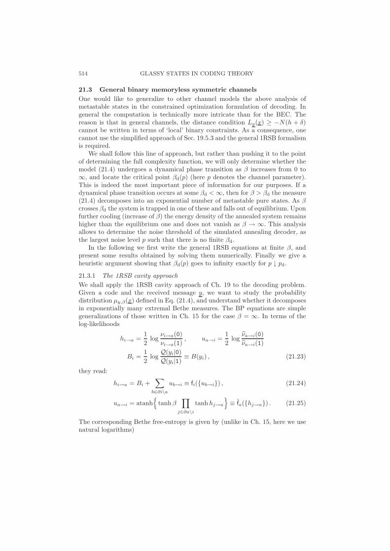
514 GLASSY STATES IN CODING THEORY
21.3 General binary memoryless symmetric channels
One would like to generalize to other channel models the above analysis ofmetastable states in the constrained optimization formulation of decoding. Ingeneral the computation is technically more intricate than for the BEC. Thereason is that in general channels, the distance condition Ly(x) ≥ −N(h + δ)cannot be written in terms of ‘local’ binary constraints. As a consequence, onecannot use the simplified approach of Sec. 19.5.3 and the general 1RSB formalismis required.
We shall follow this line of approach, but rather than pushing it to the pointof determining the full complexity function, we will only determine whether themodel (21.4) undergoes a dynamical phase transition as β increases from 0 to∞, and locate the critical point βd(p) (here p denotes the channel parameter).This is indeed the most important piece of information for our purposes. If adynamical phase transition occurs at some βd < ∞, then for β > βd the measure(21.4) decomposes into an exponential number of metastable pure states. As βcrosses βd the system is trapped in one of these and falls out of equilibrium. Uponfurther cooling (increase of β) the energy density of the annealed system remainshigher than the equilibrium one and does not vanish as β → ∞. This analysisallows to determine the noise threshold of the simulated annealing decoder, asthe largest noise level p such that there is no finite βd.
In the following we first write the general 1RSB equations at finite β, andpresent some results obtained by solving them numerically. Finally we give aheuristic argument showing that βd(p) goes to infinity exactly for p ↓ pd.
21.3.1 The 1RSB cavity approach
We shall apply the 1RSB cavity approach of Ch. 19 to the decoding problem.Given a code and the received message y, we want to study the probabilitydistribution µy,β(x) defined in Eq. (21.4), and understand whether it decomposesin exponentially many extremal Bethe measures. The BP equations are simplegeneralizations of those written in Ch. 15 for the case β = ∞. In terms of thelog-likelihoods
hi→a =1
2log
νi→a(0)
νi→a(1), ua→i =
1
2log
νa→i(0)
νa→i(1)
Bi =1
2log
Q(yi|0)Q(yi|1)
≡ B(yi) , (21.23)
they read:
hi→a = Bi +∑
b∈∂i\a
ub→i ≡ fi(ub→i) , (21.24)
ua→i = atanh
tanhβ∏
j∈∂a\i
tanhhj→a
≡ fa(hj→a) . (21.25)
The corresponding Bethe free-entropy is given by (unlike in Ch. 15, here we usenatural logarithms)

GENERAL BINARY MEMORYLESS SYMMETRIC CHANNELS 515
F(u, h) = −∑
(ia)∈E
log
[∑
xi
νua→i(xi)νhi→a(xi)
]+
N∑
i=1
log
[∑
xi
Q(yi|xi)∏
a∈∂i
νua→i(xi)
]
+M∑
a=1
log
∑
x∂a
exp(−βEa(x∂a))∏
i∈∂a
νhi→a(xi)
. (21.26)
As in (15.44), we shall introduce a “shifted” free-entropy density φ defined as
φ =1
NF(u, h) −
∑
y
Q(y|0) logQ(y|0) , (21.27)
Recall that the 1RSB cavity approach assumes that, to leading exponentialorder, the number N (φ) of Bethe measures with a shifted free-entropy densityequal to φ is equal to the number of quasi-solutions of Eqs. (21.24), (21.25).We shall write as usual N (φ)
.= exp(NΣ(φ)), and our aim is to compute the
complexity Σ(φ), using as in Ch. 19 an auxiliary graphical model which countsthe number of solutions of BP equations, weighted by a factor exp(Nxφ). If thefree-entropy of the auxiliary model is F(x) = limN→∞ FRSB(x)/N , then Σ(φ) isgiven by the Legendre transform F(x) = xφ + Σ(φ), ∂Σ/∂φ = −x.
For a given code and received y, the basic objects involved in the 1RSBapproach are the distributions of the fields hi→a and ub→j denoted respectively
as Qia and Qbj . They satisfy the following 1RSB equations:
Qia(hi→a) ∼=∫
δ (hi→a = fi(ub→i)) (zia)x∏
b∈∂i\a
dQbi(ub→i) , (21.28)
Qai(ua→i) ∼=∫
δ(ua→i = fa(hj→a)
)(zai)
x∏
j∈∂a\i
dQja(hj→a) . (21.29)
Exercise 21.8 Show that the factors zia and zai in these equations, definedin (19.23), (19.24), are given by:
zia(ub→i, Bi) =2 cosh(Bi +
∑b∈∂i\a ub→i)∏
b∈∂i\a(2 cosh(ub→i)), (21.30)
zai(hj→a) = 1 + e−2β . (21.31)
Although in this case zai is a constant and can be absorbed in the normal-ization, we shall keep it explicitly in the following.
We now turn to the statistical analysis of these equations. Picking up a uni-formly random edge in the Tanner graph of a code from the LDPCN (Λ, P ) en-semble, the densities Q and Q become themselves random objects which satisfythe distributional equations:

516 GLASSY STATES IN CODING THEORY
Q(h)d=
1
Z
∫z(ua; B(y))x δ
(h− fl−1(ua; B(y))
) l−1∏
a=1
dQa(ua) , (21.32)
Q(u)d=
1
Z
∫z(hi)x δ
(u − fk−1(hi)
) k−1∏
i=1
dQi(hi) . (21.33)
where k, l, y are random variables, Qa are l − 1 i.i.d. copies of Q, and Qiare k−1 i.i.d. copies of Q. Further, l is drawn from the edge perspective variabledegree profile λ, k is drawn from the edge perspective check degree profile ρ,and y is drawn from Q( · |0), the distribution of channel output upon input 0.
The functions fk−1(hi) = atanh(tanhβ∏k−1
i=1 tanh(hi)), and fl−1(ua; B) =
B−∑l−1
a=1 ua are defined analogously to Eqs. (21.24), (21.25). The functions z( · )and z( · ) are given similarly by the expressions in (21.30), (21.31).
The 1RSB free-entropy density (i.e. the entropy density of the auxiliarymodel) is estimated as F(x) = fRSB(Q, Q) where fRSB(Q, Q) is the expected free-entropy density and Q and Q are distributed according to the ‘correct’ solutionof the distributional equations Eqs. (21.32), (21.33).
fRSB(Q, Q) = −Λ′(1) E log ze(Q, Q) + E log zv(Qa; l, y) +Λ′(1)
P ′(1)E log zf(Qi; k) .
Here the expectation is taken with respect to k i.i.d. copies of Q and l i.i.d. copies
of Q, and with respect to kd= P·, l
d= Λ· and y
d= Q( · |0). Finally, ze, zv, zf read:
ze(Q, Q) =
∫dQ(h) dQ(u)
[ 1∑
x=0
νh(x)νu(x)]x
, (21.34)
zv(Qa; l, y) =
∫ l∏
a=1
dQa(ua)[ 1∑
x=0
Q(y|x)
Q(y|0)
l∏
a=1
νua(x)]x
, (21.35)
zf(Qi; k) =
∫ l∏
i=1
dQi(hi)[ ∑
x1,··· ,xk
k∏
i=1
νhi(xi)
(I(∑
i
xi = even)
+ e−2β I(∑
i
xi = odd))]x
.(21.36)
A considerable amount of information is contained in the 1RSB free-energy den-sity F(x). For instance, one could deduce from it the energetic complexity bytaking the appropriate β → ∞ limit. Here we shall not attempt at developinga full solution of the 1RSB distributional equations, but use them to detect theoccurrence of a dynamical phase transition.
21.3.2 Dynamical phase transition
The location of the dynamical phase transition location βd(p) is determined asthe smallest value of β such that the distributional equations (21.32), (21.33)

GENERAL BINARY MEMORYLESS SYMMETRIC CHANNELS 517
0.00
0.02
0.04
0.06
0.08
0.10
0 0.1 0.2 0.3 0.4 0.50
0.02
0.04
0.06
0.08
0.1
0.12
0.14
0.16
0.18
0 0.05 0.1 0.15 0.2 0.25 0.3 0.35 0.4 0.45 0.5
BSCτ = 10
τ = 102
τ = 103εd ( Td )
p
e−2β
pd
p
eann
pd
Fig. 21.6. Left: Dynamic phase transition for random codes from the (5, 6) en-semble used over the BSC(p) (circles are obtained through sampled densityevolution; the dashed line is a guide for the eye). Right: residual energy den-sity after simulated annealing, as measured in numerical simulations. Thedashed line gives the equilibrium energy at the dynamical transition temper-ature Td.
have a non-trivial solution at x = 1. For β > βd(p), the distribution (21.4)decomposes into an exponential number of pure states. As a consequence, weexpect simulated annealing to fall out of equilibrium when βd(p) is crossed.
In Fig. 21.6 left frame, we show the result of applying such a technique tothe (5, 6) regular ensemble used for communication over the BSC(p). At small p,no dynamic phase transition is revealed through this procedure at any positivetemperature. Above a critical value of the noise level p, the behavior changesdramatically and a phase transition is encountered at a critical point βd(p) thatdecreases monotonically for larger p. By changing both β and p, one can iden-tify a phase transition line that separates the ergodic and non-ergodic phases.Remarkably, the noise level at which a finite βd appears is numerically indistin-guishable from pd ≈ 0.145.
Does the occurrence of a dynamical phase transition for p # pd indeed influ-ence the behavior of the simulated annealing decoder? Some numerical confir-mation was already presented in Fig. 21.2. Further support in favor of this thesisis provided by Fig. 21.6, right frame, which plots the residual energy density ofthe configuration produced by the decoder as β → ∞. Above pd this becomesstrictly positive and only slowly dependent on the cooling rate. It is comparedwith the equilibrium value of the internal energy at βd(p). This would be thecorrect prediction if the system didn’t decrease any more its energy after it fallsout of equilibrium at βd(p). Although we do not expect this to be strictly true,the resulting curve provides a good first estimate.

518 GLASSY STATES IN CODING THEORY
21.3.3 Metastable states and BP threshold
One crucial element of this picture can be confirmed analytically, for a genericBMS channel family ordered by physical degradation with respect to p: At zerotemperature, the dynamical transition, signaling the proliferation of metastableBethe states, occurs exactly at the decoding threshold pd. More precisely, theargument below proves that at β = ∞ there cannot exist any non-trivial x = 1solution of Eqs. (21.32), (21.33) for p < pd, while there exists one for p > pd.We expect that, for most channel families, the same situation should hold for βlarge enough (and dependent on p), but this has not been proven yet.
Let us consider the 1RSB equations (21.32), (21.33) in the case β = ∞.Assuming that the degree profiles are such that l ≥ 2 and k ≥ 2 (a reasonablerequirement for useful code ensembles), it is clear that they have a special ‘no-error’ solution associated with the sent codeword in which Q(h) = δ∞(h) andQ(u) = δ∞(h) almost surely. It is a simple exercise to check that the (shifted)free-entropy density of this solution is equal to 0.
The important question is whether there exist other solutions beyond the ‘no-error’ one. We can make use of the simplification occuring at x = 1. As we saw inSec. 19.4.1, the expectation values of the messages, νav
i→a(xi) ≡∑
νiaQia(νia)νia(xi)
and νava→i(xi) ≡
∑bmai
Qai(νai)νai(xi) satisfy the BP equations.Let us first study the case p < pd. We have seen in Ch. 15 that there is a
unique solution of BP equations: the no-error solution. This shows that in thislow noise regime, there cannot exist any non-trivial 1RSB solution. We concludethat there is no glass phase in the regime p < pd
We now turn to the case p > pd (always with β = ∞), and use the analysis ofBP presented in Ch. 15. That analysis revealed that, when p > pd, the densityevolution of BP messages admits at least one ‘replica symmetric’ fixed pointdistinct from the no-error one.
We shall now use this replica symmetric fixed point in order to construct anon-trivial 1RSB solution. The basic intuition behind this construction is thateach Bethe measure consists of a single configuration, well separated from otherones. Indeed, each Bethe measure can be identified with a zero-energy configura-tion, i.e. with a codeword. If this is true, then, with respect to each of these Bethemeasures the local distribution of a variable is deterministic, either a unit masson 0 or a unit mass on 1. Therefore we seek a solution where the distribution ofQ and Q is supported on functions of the form:
Q(h) =1
2(1 + tanh h) δ+∞(h) +
1
2(1 − tanh h) δ−∞(h) , (21.37)
Q(u) =1
2(1 + tanh u) δ+∞(u) +
1
2(1 + tanh u) δ−∞(u) , (21.38)
where h and u are random variables.

GENERAL BINARY MEMORYLESS SYMMETRIC CHANNELS 519
Exercise 21.9 Show that this Ansatz solves Eqs. (21.32), (21.33) at β = ∞ ifand only if the distributions of h, u satisfy:
hd= B(y) +
l−1∑
a=1
u , ud= atanh
[ k−1∏
i=1
tanh hi
]. (21.39)
It is easy to check that the random variables h and u satisfy the same equa-tions as the fixed point of density evolution for BP (see Eq. (15.11)). We concludethat, for p > pd and x = 1, a solution to the 1RSB equations is given by theAnsatz (21.37), (21.38), if h, u are drawn from the fixed point distributions ofEq. (15.11).
It turns out that a similar solution is easily found for any value of x > 0,provided β = ∞. The only place where x plays a role is in the reweighting factorof Eq. (21.35): when x .= 1, the only modification in the distributional equations(21.39) is that B(y) should be multiplied by x. Therefore one can obtain the 1RSBsolution for any x > 0 if one knows the solution to the RS cavity equations (i.e.the fixed point of the density evolution for BP) in a slightly modified problem inwhich B(y) is changed to xB(y). Technically this is equivalent to studying themodified measure
µy(x) ∼=M∏
a=1
I(xia1⊕ · · ·⊕ xia
k(a)= 0)
N∏
i=1
Q(yi|xi)x , (21.40)
within the RS approach of Ch. 15 (such a modified measure was already intro-duced in Ch. 6).
Let us assume that we have found a non-trivial fixed point for this aux-
iliary problem, characterized by the distributions a(x)RS(h), and a
(x)RS(u), and call
fRS(x) the corresponding value of the free-entropy density defined in (15.45). The1RSB equations with reweighting parameter x have a solution of the type (21.37),
(21.38), provided h is distributed according to a(x)RS( · ), and u is distributed ac-
cording to a(x)RS( · ). The 1RSB free-entropy density F(x) = E FRSB(x)/N is simply
given by:F(x) = fRS(x) . (21.41)
Therefore the problem of computing F(x), and its Legendre transform the com-plexity Σ(φ), reduce to a replica symmetric computation. This is a simple gen-eralization of the problem Ch. 15, whereby the decoding measure is modified byraising it to the power x, as in Eq. (21.40). Notice however that the interpreta-tion is now different. In particular x has to be properly chosen in order to focuson dominant pure states.
The problem can be easily studied numerical using the population dynamicsalgorithm. Fig. 21.7 shows an example of the complexity Σ(φ) for a BSC channel.

520 GLASSY STATES IN CODING THEORY
-0.05
0
0.05
0.1
0.15
0 0.2 0.4 0.6 0.8 1 1.2 1.4 1.6 0
0.05
0.1
0.15
0.2
-0.2 -0.15 -0.1 -0.05 0 0.05φ
Σ(φ)
x
F(x)
Fig. 21.7. Left: The free-entropy of the auxiliary model, F(x), as a func-tion of the weight parameter x, for a (3, 6) code on the BSC chan-nel (recall that pd ≈ 0.084 and pc ≈ 0.101 in this case). From bot-tom to top: p = 0.090, 0.095, 0.100, 0.105, 0.110. Right: The complexityΣ(φ) plotted versus the shifted free-entropy density φ. From left to right:p = 0.090, 0.095, 0.100, 0.105, 0.110.
The regime pd < p < pc is characterized by the existence of a band of metastablestates with negative shifted free-entropy φ ≤ φ0 < 0. They are in principleirrelevant when compared to the ‘no-error’ solution which has φ = 0, confirmingthat MAP decoding will return the transmitted codeword. In fact they are evenunphysical: φ is nothing but the conditional entropy density of the transmittedcodeword given the received message. As a consequence it must be non-negative.However the solution extends to β < ∞, where it makes perfect sense (it describesnon-codeword metastable configurations), thus solving the puzzle.
The appearance of metastable states coincides with the noise threshold abovewhich BP decoding fails. When p > pc the top end of the band φ0 becomespositive: the ‘glassy’ states dominate the measure and MAP decoding fails.
21.4 Metastable states and near-codewords
In a nutshell, the failure of BP decoding for p > pd can be traced back toconfigurations (words) x that: (i) Are deep local minima of the energy functionE(x) (that counts the number of violated parity checks); (ii) Have a significantweight under the measure
∏i Q(y|xi).
Typically, such configurations are not codewords, although they can be veryclose to codeword from the energy point of view. An interesting qualitative anal-ogy can be drawn between this analysis, and various notions that have beenintroduced to characterize the so-called error floor.
Let us start by describing the error floor problem. We saw that for p < pd
the bit error rate under BP decoding vanishes when the blocklength N → ∞.Unhappily, the blocklength cannot be taken arbitrarily large because of two typesof practical considerations. First, coding a block of N bits simultaneously impliesa communication delay proportional to N . Second, any hardware implementation
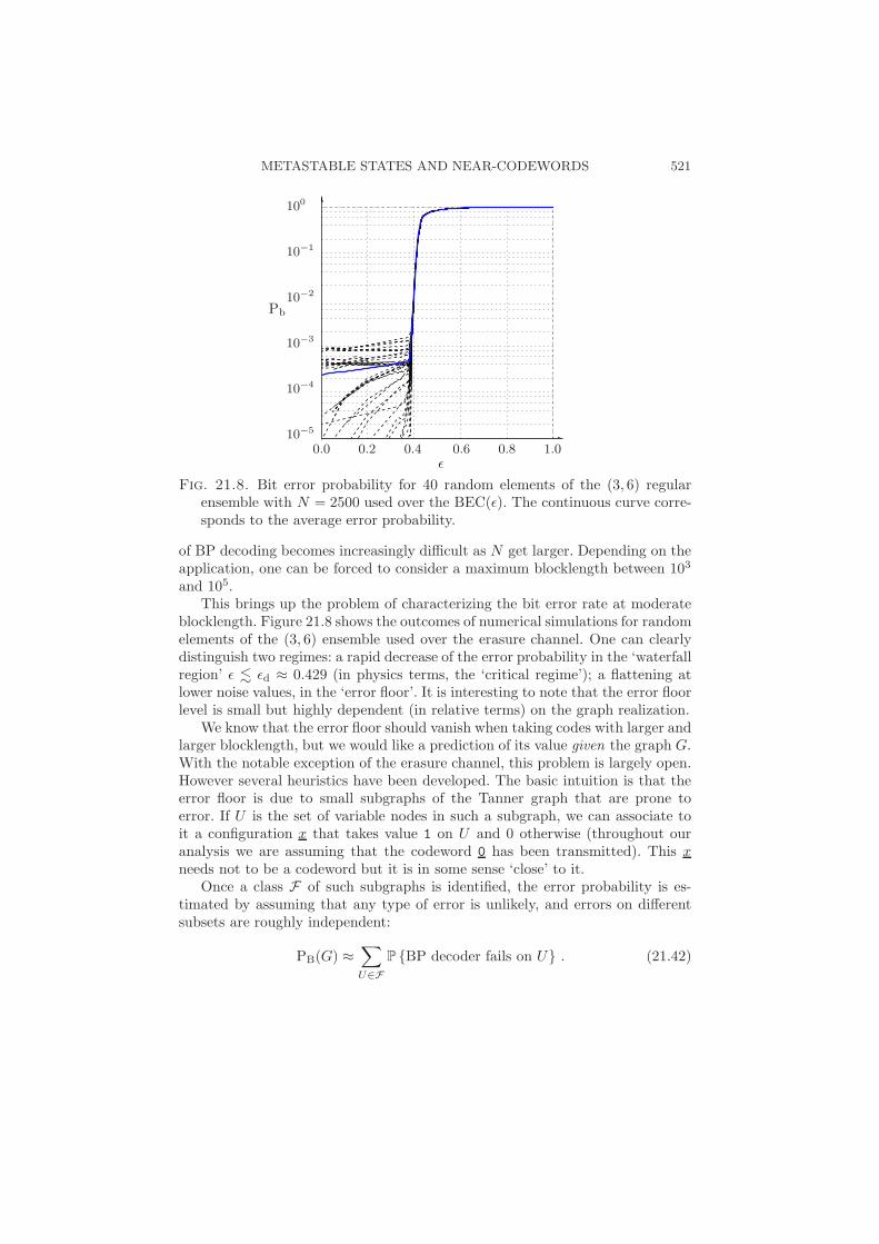
METASTABLE STATES AND NEAR-CODEWORDS 521
0.0 0.2 0.4 0.6 0.8 1.0
100
10−1
10−2
10−3
10−4
10−5
ε
Pb
Fig. 21.8. Bit error probability for 40 random elements of the (3, 6) regularensemble with N = 2500 used over the BEC(ε). The continuous curve corre-sponds to the average error probability.
of BP decoding becomes increasingly difficult as N get larger. Depending on theapplication, one can be forced to consider a maximum blocklength between 103
and 105.This brings up the problem of characterizing the bit error rate at moderate
blocklength. Figure 21.8 shows the outcomes of numerical simulations for randomelements of the (3, 6) ensemble used over the erasure channel. One can clearlydistinguish two regimes: a rapid decrease of the error probability in the ‘waterfallregion’ ε " εd ≈ 0.429 (in physics terms, the ‘critical regime’); a flattening atlower noise values, in the ‘error floor’. It is interesting to note that the error floorlevel is small but highly dependent (in relative terms) on the graph realization.
We know that the error floor should vanish when taking codes with larger andlarger blocklength, but we would like a prediction of its value given the graph G.With the notable exception of the erasure channel, this problem is largely open.However several heuristics have been developed. The basic intuition is that theerror floor is due to small subgraphs of the Tanner graph that are prone toerror. If U is the set of variable nodes in such a subgraph, we can associate toit a configuration x that takes value 1 on U and 0 otherwise (throughout ouranalysis we are assuming that the codeword 0 has been transmitted). This xneeds not to be a codeword but it is in some sense ‘close’ to it.
Once a class F of such subgraphs is identified, the error probability is es-timated by assuming that any type of error is unlikely, and errors on differentsubsets are roughly independent:
PB(G) ≈∑
U∈FP BP decoder fails on U . (21.42)

522 GLASSY STATES IN CODING THEORY
If the subset U are small, each of the terms on the right hand side can beevaluated efficiently via importance sampling.
It is interesting to have a look at some definitions of the class of subgraphs Fthat have been introduced in the literature. In each case the subgraph is char-acterized by two integers (w, e) that describe how dangerous/close to codewordsthey are (small w or e corresponding to dangerous subgraphs). In practice onerestricts the sum in Eq. (21.42) to small w, e.
Trapping sets. (or near codewords) A trapping set is a subgraph includingthe variable nodes in U , all the adjacent check nodes and the edges that connectthem. It is a (w, e) near-codeword if the number of variable nodes is |U | = wand the number of check nodes of odd degree is e.
In our framework a trapping set is simply a configuration x with weight(number of non-zero entries) equal to w and energy E(x) = 2e. Notice that hardlyany restriction is imposed on trapping sets. Special constraints are sometimesadded depending on the channel model, and on the decoding algorithm (if notBP).
Adsorbing sets. A (w, e) adsorbing set is a (w, e) trapping set that satisfiestwo further requirements: (i) Each variable node is adjacent to more check nodesof even degree (with respect to the subgraph) than of odd degree; (ii) It doesnot contain a (w′, e) adsorbing set with w′ < w.
The first condition implies that the corresponding configuration x is a localminimum of E(x) stable with respect to 1 flip.
The connection between small weak subgraphs and error probability is stillsomewhat vague. The ‘energy landscape’ E(x) might provide some hints towardsbridging this gap.
Notes
This chapter is largely based on the analysis of metastable states in (Montanari,2001b), (Montanari, 2001a) and (Franz, Leone, Montanari and Ricci-Tersenghi,2002). One step replica symmetry breaking was also investigated in (Miglioriniand Saad, 2006). The approach was extended to asymmetric channels in (Neri,Skantzos and Bolle, 2008).
Typical pairs decoding presented here is slightly different from the originalprocedure of (Aji, Jin, Khandekar, MacKay and McEliece, 2001).
Stopping sets were introduced in (Di, Proietti, Richardson, Telatar and Ur-banke, 2002), and inspired much of the subsequent research on error floors. Theidea that small subgraphs of the Tanner graph are responsible for error floorswas first convincingly demonstrated for general channel models in (MacKay andPostol, 2003) and (Richardson, 2003). Absorbing sets are defined in (Dolecek,Zhang, Anantharam and Nikolic, 2007).
After its invention, simulated annealing was the object of a significant amountof work within operations research and probability. A review can be found in

NOTES 523
(Aarts, Korst and van Laarhoven, 2003). A detailed comparison between 1RSBanalysis and simulated annealing experiments for models on sparse graphs ispresented in (Montanari and Ricci-Tersenghi, 2004).

22
AN ONGOING STORY
This book describes a unified approach to a number of important problems ininformation theory, physics and computer science. We have presented a consistentset of methods to address these problems, but the field is far from being fullyunderstood, and there remain many open challenges. This chapter provides asynthetic description of some of these challenges, as well as a survey of recentprogress. Our ambition is to set an agenda for the newly developed field that wehave been describing. We will distinguish roughly three types of directions.
The first one, to be discussed in Sec. 22.1, is the main challenge. It aims ata better qualitative understanding of models on sparse random graphs. At thecore of the cavity method lies the postulate that such systems can have only alimited number of ‘behaviors’ (phases). Each phase corresponds to a differentpattern of replica symmetry breaking (replica symmetric -RS, one-step replicasymmetry breaking -1RSB, etc. . . ). In turn they also have a description in termsof pure states decomposition, as well as in terms of long range correlations.Understanding the fundamental reasons and conditions for the universality ofthese phases, as well as the equivalence among their characterizations would beextremely important.
The second direction, described in Sec. 22.2, concerns the development of thecavity formalism itself. We have mainly focused on systems in which either theRS or 1RSB cavity method is expected to be asymptotically exact in the largesize limit. This expectation is in part based on some internal consistency checksof the 1RSB approach. An important one consists in verifying that the 1RSB‘solution’ is stable with respect to small perturbations. Whenever this test ispassed, physicists feel confident enough that the cavity method provides exactconjectures (thresholds, minimum cost per variable, etc. . . ). If the test is notpassed, higher order RSB is thought to be needed. The situation is much lesssatisfactory in this case, and the cavity method poses some technical problemseven at the heuristic level.
Section 22.3 lists a number of fascinating questions that arise in the connexionbetween the existence of glassy phase transitions and algorithmic slowdown.These are particularly important in view of the applications in computer scienceand information theory: sparse graphical models can be useful for a number ofpractically relevant tasks, as the example of LDPC codes in channel coding hasshown. There is some empirical evidence that phase transitions have an impacton algorithms behavior and efficiency. Physicists hope that this impact can beunderstood (to some extent) in a unified way, and is ultimately related to thegeometric structure of the set of solutions, and to correlation properties of the
524

GIBBS MEASURES AND LONG-RANGE CORRELATIONS 525
measure. While some general arguments in favour of this statement have beenput forward, the actual understanding is still very poor.
22.1 Gibbs measures and long-range correlations
At an abstract level, the cavity method explored in the last few chapters relieson a (yet unproven) structural theorem. Consider a generic graphical model, aprobability distribution on N variables, x, taking values in a discrete space XN :
µ(x) =1
Z
∏
a∈F
ψa(x∂a) . (22.1)
The cavity method postulates that, for large classes of models taken from someappropriate ensembles, the model is qualitatively described in the large N limitby one out of a small number of generic scenarios, or phases. The postulatedqualitative features of such phases are then cleverly used to derive quantitativepredictions (e.g. phase transition locations.)
Needless to say, we are not able to state precisely, let alone to prove, such astructural theorem in this generality. The complete set of necessary hypotheses isunknown. However we discussed several examples, from XORSAT to diluted spinglasses or error correcting codes. In principle, it is not necessary that the factorgraph be locally tree-like, but in practice locally tree-like models are the onesthat we can control most effectively. Such a structure implies that when one digsa cavity in the graph, the variables on the boundary of the cavity are far apart.This leads to a simple structure of their correlation in the large system limit,and hence to the possibility of writing asymptotically exact recursion equations.
Here we do not want to discuss in more details the hypotheses. It wouldcertainly be a significant achievement to prove such a structural theorem evenin a restricted setting (say, for the uniform measure over solutions of random K-SAT formulae). We want instead to convey some important features of the phasespostulated within the cavity approach. In particular there is a key aspect thatwe want to stress. Each of the various phases mentioned can be characterizedfrom two, complementary, points of view:
1. In terms of decomposition of the distribution µ( · ) into ‘lumps’ or ‘clusters’.Below we shall propose a precise definition of the lumps, and they will becalled pure states.
2. In terms of correlations among far apart variables on the factor graph.We shall introduce two notions of correlation decay that differ in a rathersubtle way but correspond to different phases.
These two characterizations are in turn related to the various aspects of thecavity method.
22.1.1 On the definition of pure states
The notion of pure state is a crucial one in rigorous statistical mechanics. Un-fortunately, standard definitions are tailored to translation-invariant models on
526 AN ONGOING STORY
infinite graphs. The graphical models that we have in mind are sparse randomgraphs (in this class we include labeled random graphs, whereby the labels spec-ify the nature of function nodes), and standard approaches don’t apply to them.In particular, we need a concrete definition that is meaningful for finite graphs.
Consider a sequence of finite graphical models µN ( · ), indexed by the num-ber of variable nodes N . A pure state decomposition is defined by assign-ing, for each N , a partition of the configuration space XN into NN subsetsΩ1,N , . . . ,ΩNN ,N :
XN = Ω1,N ∪ · · · ∪ ΩNN ,N . (22.2)
The pure state decomposition must meet the following conditions:
1. The measure of each subset in the partition is bounded away from 1:
maxµN(Ω1,N ), . . . , µN (ΩN ,N ) ≤ 1 − δ . (22.3)
2. The subsets are separated by ‘bottlenecks.’ More precisely, for Ω ⊆ XN ,define its ε-boundary as
∂εΩ ≡ x ∈ XN : 1 ≤ d(x,Ω) ≤ Nε . (22.4)
where d(x,Ω) is the minimum Hamming distance between x and any con-figuration x′ ∈ Ω. Then we require
limN→∞
maxr
µN (∂εΩr,N)
µN (Ωr,N )= 0 , (22.5)
for some ε > 0. Notice that the measure of ∂εΩr,N can be small for two rea-sons, either because Ωr,N is small itself (and therefore has a small bound-ary) or because the boundary of Ωr,N is much smaller than its interior.Only the last situation corresponds to a true bottleneck, as is enforced bythe denominator µN (Ωr,N ) in (22.5).
3. The conditional measure on the subset Ωr,N , defined by
µrN (x) ≡ 1
µN (Ωr,N )µN (x)I(x ∈ Ωr,N ) (22.6)
cannot be further decomposed according to the two conditions above.
Given such a partition, the distribution µN ( · ) can be written as a convexcombination of distributions with disjoint support
µN ( · ) =NN∑
r=1
wr µrN ( · ) , wr ≡ µN (Ωr,N ) . (22.7)
Notice that this decomposition is not necessarily unique, as shown by the examplebelow. Non-uniqueness is due to the fact that sets of configurations of XN withnegligeable weight can be attributed to one state or another. On the other hand,the conditional measures µr
N ( · ) should depend weakly on the precise choice ofdecomposition.
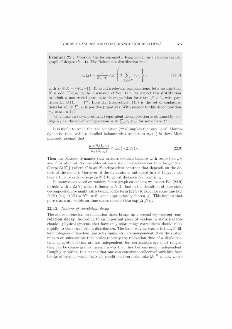
GIBBS MEASURES AND LONG-RANGE CORRELATIONS 527
Example 22.1 Consider the ferromagnetic Ising model on a random regulargraph of degree (k + 1). The Boltzmann distribution reads
µN (x) =1
ZN(β)exp
β∑
(i,j)∈E
xixj
, (22.8)
with xi ∈ X = +1,−1. To avoid irrelevant complications, let’s assume thatN is odd. Following the discussion of Sec. 17.3, we expect this distributionto admit a non-trivial pure state decomposition for k tanhβ > 1, with par-tition Ω+ ∪ Ω− = XN . Here Ω+ (respectively Ω−) is the set of configura-tions for which
∑i xi is positive (negative). With respect to this decomposition
w+ = w− = 1/2.Of course an (asymptotically) equivalent decomposition is obtained by let-
ting Ω+ be the set of configurations with∑
i xi ≥ C for some fixed C.
It is useful to recall that the condition (22.5) implies that any ‘local’ Markovdynamics that satisfies detailed balance with respect to µN ( · ) is slow. Moreprecisely, assume that
µN (∂εΩr,N )
µN (Ωr,N )≤ exp−∆(N) . (22.9)
Then any Markov dynamics that satisfies detailed balance with respect to µN
and flips at most Nε variables at each step, has relaxation time larger thanC exp∆(N) (where C is an N -independent constant that depends on the de-tails of the model). Moreover, if the dynamics is initialized in x ∈ Ωr,N , it willtake a time of order C exp∆(N) to get at distance Nε from Ωr,N .
In many cases based on random factor graph ensembles, we expect Eq. (22.9)to hold with a ∆(N) which is linear in N . In fact in the definition of pure statedecomposition we might ask a bound of the form (22.9) to hold, for some function∆(N) (e.g. ∆(N) = Nψ, with some appropriately chosen ψ). This implies thatpure states are stable on time scales shorter than exp∆(N).
22.1.2 Notions of correlation decay
The above discussion on relaxation times brings up a second key concept: cor-relation decay. According to an important piece of wisdom in statistical me-chanics, physical systems that have only short-range correlations should relaxrapidly to their equilibrium distribution. The hand-waving reason is that, if dif-ferent degrees of freedom (particles, spins, etc) are independent, then the systemrelaxes on microscopic time scales (namely the relaxation time of a single par-ticle, spin, etc). If they are not independent, but correlations are short ranged,they can be coarse grained in such a way that they become nearly independent,Roughly speaking, this means that one can construct ‘collective’ variables fromblocks of original variables. Such conditional variables take |X |B values, where

528 AN ONGOING STORY
B is the block size, and are nearly independent under the original (Boltzmann)distribution.
As we are interested in models on non-Euclidean graphs, the definition ofcorrelation decay must be precised. We will introduce two distinct types of cri-teria. Although they may look similar at first sight, it turns out that they arenot, and each of them will characterize a distinct generic phase.
The simplest approach, widely used in physics, consists in considering two-points correlation functions. Averaging them over the two positions defines asusceptibility. For instance, in the case of Ising spins xi ∈ X = 1,−1, we havealready discussed the spin glass susceptibility
χSG =1
N
∑
i,j∈V
(〈xixj〉 − 〈xi〉〈xj〉)2 , (22.10)
where 〈 · 〉 denotes the expectation value with respect to µ. When χSG is boundedas N →∞, this is an indication of short range correlations. Through the fluctua-tion dissipation theorem (cf. Sec. 2.3), this is equivalent to stability with respectto local perturbations. Let us recall the mechanism of this equivalence. Imaginea perturbation of the model (22.16) that acts on a single variable xi. Stabilityrequires that the effect of such a perturbation on the expectation of a global ob-servable
∑j f(xj) should be bounded. The change in the marginal at node j due
to a perturbation at i, is proportional to the covariance 〈xixj〉 − 〈xi〉〈xj〉. As inSec. 12.3.2, the average effect of the perturbation at i on the variables xj , j .= ioften vanishes (more precisely limN→∞
1N
∑j∈V
(〈xixj〉−〈xi〉〈xj〉
)= 0) because
terms related to different vertices j cancel. The typical effect of the perturbationis captured by the spin glass-susceptibility.
Generalizing this definition to arbitrary alphabets is easy. We need to use ameasure of how much the joint distribution µij( · , · ) of xi and xj is different fromthe product of the marginals µi( · ) times µj( · ). One such measure is providedby the variation distance:
||µij( · , · )− µi( · )µj( · )|| ≡1
2
∑
xi,xj
|µij(xi, xj) − µi(xi)µj(xj)| . (22.11)
We then define the two-points correlation by averaging this distance over thevertices i, j
χ(2) ≡ 1
N
∑
i,j∈V
||µij( · , · )− µi( · )µj( · )|| . (22.12)
Exercise 22.1 Consider again the case of Ising variables, X = +1,−1. Showthat χSG = o(N) if and only if χ(2) = o(N).
[Hint: Let Cij ≡ 〈xixj〉 − 〈xi〉〈xj〉. Show that Cij = 2||µij( · , · ) −µi( · )µj( · )||. Then use χSG = NEC2
ij, χ(2) = NE|Cij |/2, the expectationE being over uniformly random i, j ∈ V .]

GIBBS MEASURES AND LONG-RANGE CORRELATIONS 529
Of course one can define l-points correlations in an analogous manner:
χ(l) ≡ 1
N l−1
∑
i(1),...,i(l)∈V
||µi(1)...i(l)( · · · ) − µi(1)( · ) · · ·µi(l)( · )|| . (22.13)
The l-points correlation χ(l) has a useful interpretation in terms of a thoughtexperiment. Suppose you are given an N -dimensional distribution µ(x) and haveaccess to the marginal µi(1)( · ) at a uniformly random variable node i(1). Youwant to test how stable is this marginal with respect to small perturbations.Perturbations affect l− 1 randomly chosen variable nodes i(2),. . . , i(l) changingµ(x) into µ′(x) ∼= µ(x)(1 + δ2(xi(2))) · · · (1 + δl(xi(l))). The effect of the resultingperturbation on µi(1), to the first order in the product δ2 · · · δl, is bounded in
expectation by χ(l) (this is again a version of the fluctuation dissipation theorem).
Definition 22.2. (First type of correlation decay) The graphical model givenby µ( · ) is said to be stable to small perturbations if, for all finite l, χ(l)/N →0 as N →∞.
In practice in sufficiently homogeneous (mean field) models, this type of stabilityis equivalent to the one found using only l = 2.
Let us now introduce another type of criterion for correlation decay. Again welook at a variable node i, but now we want to check how strongly xi is correlatedwith all the ‘far apart’ variables. Of course we must define what ‘far apart’ means.Fix an integer - and define B(i, -) as the ball of radius - centered at i, and B(i, -)its complement, i.e. the subset of variable nodes j such that d(i, j) ≥ -. We thenwant to estimate the correlation between xi and x
B(i,%) = xj : j ∈ B(i, -). This
amounts to measuring the distance between the joint distribution µi,B(,%)( · , · )and the product of the marginals µi( · )µB(,%)( · ). If we use the total variation
distance defined in (22.11) we obtain the following point-to-set correlationfunction
Gi(-) ≡ ||µi,B(i,%)( · , · ) − µi( · )µB(i,%)( · )|| . (22.14)
The function Gi(-) can be interpreted according to two distinct but equallysuggestive thought experiments. The first one comes from the theory of struc-tural glasses (it is meant to elucidate the kind of long range correlations arisingin a fragile glass). Imagine to draw a reference configuration x∗ from the distri-bution µ( · ). Now generate a second configuration x as follows: variables outsidethe ball, with i ∈ B(i, -), are forced to the reference configuration: xi = x∗
i .Variables at distance smaller than - (denoted by xB(i,%)) are instead drawn fromthe conditional distribution µ(xB(i,%)|x∗
B(i,%)). If the model µ( · ) has some form of
rigidity (long range correlations), then xi should be close to x∗i . The correlation
Gi(-) measures how much the distributions of xi and x∗i differ.
The second experiment is closely related to the first one, but has the flavourof a statistics (or computer science) question. Someone draws the configuration

530 AN ONGOING STORY
x∗ as above from the distribution µ( · ). She then reveals to you the values of farapart variables in the reference configuration, i.e. the values x∗
j for all j ∈ B(i, -).She asks you to reconstruct the value of x∗
i , or to guess it as well as you can.The correlation function Gi(-) measures how likely you are to guess correctly(assuming unbounded computational power), compared to the case in which no-variable has been revealed to you.
This discussion suggests the following definition:
Definition 22.3. (Second type of correlation decay) The graphical modelµ( · ) is said to satisfy the non-reconstructibility (or extremality) conditionif for all i’s, Gi(-) → 0 as - →∞. (More precisely, we require that there exists afunction δ(-), with lim%→∞ δ(-) = 0, such that Gi(-) ≤ δ(-) for all i and N). Inthe opposite case, i.e. if Gi(-) remains bounded away from zero at large distance,the model is said reconstructible.
22.1.3 Generic scenarios
We shall now describe the correlation decay properties and the pure state de-composition for the three main phases that we have encountered in the previouschapters: RS, dynamical 1RSB, and static 1RSB. When dealing with models onlocally tree-like random graphs, each of these phases can also be studied usingthe appropriate cavity approach, as we shall recall.
Here we focus on phases that appear ‘generically’. This means that we ex-clude: (i) Critical points, that are obtained by fine-tuning some parameters ofthe model; (ii) Multiplicities due to global symmetries, like for instance in thezero-field ferromagnetic Ising model. Of course there also exist other types ofgeneric phases, such as higher order RSB phases that will be discussed in thenext section, and maybe some more that have not been explored yet.
Replica symmetric. In this phase there exists no non-trivial decompositioninto pure states of the form (22.7). In other words NN = 1 with high probability.
Correlations decay according to both criteria: the model is stable to smallperturbations and it satisfies the non-reconstructibility condition. Therefore it isshort-range correlated in the strongest sense.
Finally, the replica symmetric cavity method of Ch. 14 yields asymptoticallyexact predictions.
Dynamical 1RSB. In this phase the measure µ( · ) admits a non trivial de-composition of the form (22.7) into an exponential number of pure states: NN =eNΣ+o(N) with high probability for some Σ > 0. Furthermore, most of the mea-sure is carried by states of equal size. More precisely, for any δ > 0, all but anexponentially small fraction of the measure is comprised in states Ωr,N such that
−Σ− δ ≤ 1
Nlog µ(Ωr,N ) ≤ −Σ + δ . (22.15)
From the correlation point of view, this phase is stable to small perturbations,but it is reconstructible. In other words, a finite number of probes would fail to

GIBBS MEASURES AND LONG-RANGE CORRELATIONS 531
αd(K) αc(K) αs(K) α
UNSAT
Fig. 22.1. A pictorial view of the different phases in K-SAT with K ≥ 4,depending on the number of clauses per variable α. Form left to right: replicasymmetric, dynamical 1RSB, static 1RSB and UNSAT.
reveal long range correlations. But long range correlations of the point-to-settype are instead present, and they are revealed, for instance, by a slowdown ofreversible Markov dynamics.
The glass order parameter overlap distribution P (q) is trivial in this phase(as implied by (12.31)), but its glassy nature can be found through the ε-couplingmethod of Sec. 12.3.4.
The model is solved exactly (in the sense of determining its asymptotic free-energy density) within the 1RSB cavity method. The thermodynamically dom-inant states, i.e. those satisfying (22.15), correspond to the 1RSB parameterx = 1.
Static 1RSB. This is the ‘genuine’ 1RSB phase analogous to the low tem-perature phase of the random energy model. The model admits a non-trivialpure states decomposition with wildly varying weights. For any δ > 1, a frac-tion 1 − δ of the measure is comprised in the k(N, δ) pure states with largestweight. The number k(N, δ) converges, when N → ∞, to a finite random vari-able (taking integer values). If we order the weights according to their magnitudew(1) ≥ w(2) ≥ w(3) ≥ · · · , they converge to a Poisson-Dirichlet process, cf. Ch. 8.
This phase is not stable to small perturbation, and it is reconstructible: Ithas long range correlations according to both criteria. The asymptotic overlapdistribution function P (q) has two delta-function peaks, as in Fig.12.3.
Again, it is solved exactly within the 1RSB cavity method.
These three phases are present in a variety of models, and are often separatedby phase transitions. The ‘clustering’ or ‘dynamical’ phase transition separatesthe RS and dynamical 1RSB phases, while a condensation phase transition sepa-rates the dynamical 1RSB from the static 1RSB phase. Fig. 22.1.3 describes theorganization of various phases in random K-SAT with K ≥ 4, as we discussedin Sec. 20.3. For α < αd(K) the model is RS; for αd(K) < α < αc(K), it isdynamically 1RSB; for αc(K) < α < αs(K), it is statically 1RSB, for αs(K) < αit is UNSAT. Fig. 22.1.3 shows the point-to-set correlation function in random4-SAT. It clearly develops long-range correlations at α ≥ αd ≈ 9.38. Notice the

532 AN ONGOING STORY
1501209060300
0.6
0.4
0.2
0
-
Gi(-)
Fig. 22.2. The point-to-set correlation function defined in (22.14) is plottedversus distance for random 4-satisfiability, at clause densities α = 9.30, 9.33,9.35 and 9.40 (from bottom to top).
peculiar development of correlations through a plateau whose width increaseswith α, and diverges at αd. This is typical of the dynamical 1RSB transition.
22.2 Higher levels of replica symmetry breaking
For some of the models studied in this book the RS, or the 1RSB cavity methodare thought to yield asymptotically exact predictions. However, in general higherorders of RSB are necessary. We shall sketch how to construct these higherorder solutions hierarchically in locally tree-like graphical models. In particular,understanding the structure of the 2RSB solution allows to derive a ‘stabilitycriterion’ for the 1RSB approach. It is on the basis of this criterion that, forinstance, our derivation of the SAT-UNSAT threshold in Ch. 20 is conjecturedto give an exact result.
22.2.1 The high-level picture
Let us first briefly summarize the RS/1RSB approach. Consider an ensemble ofgraphical models defined through the distribution (22.1) with a locally tree-likefactor graph structure. Within the RS cavity method, the local marginals of µ( · )are accurately described in terms of the message sets νi→a, νa→i. Given asmall (tree-like) subgraph induced by the vertex set U ⊂ V , the effect of the restof the graph G \GU on U is described by a factorized measure on the boundaryof U .
One-step replica symmetry breaking relaxes this assumption, by allowing forlong-range correlations, with a peculiar structure. Namely, the probability dis-tribution µ( · ) is assumed to decompose into the convex combination of Bethemeasures µr( · ). Within each ‘state’ r, the local marginals of the measure re-stricted to this state are well described in terms of a set of messages νr
i→a(by ‘well described’ we mean that the description becomes asymptotically exactat large N). Sampling at random a state r defines a probability distribution

HIGHER LEVELS OF REPLICA SYMMETRY BREAKING 533
d0
d1d2
Fig. 22.3. Cartoon of the distribution µ(x) for a model described by two-stepreplica symmetry breaking. The probability mass is concentrated on the gray‘lumps’ of radius d2, which are organized in ‘clouds’ of radius d1 > d2. Thedashed circle corresponds to the typical distance d0 between clouds.
P(ν, ν) over messages. This distribution is then found to be described byan ‘auxiliary’ graphical model which is easily deduced from the original one. Inparticular the auxiliary factor graph inherits the structure of the original one,and therefore it is again locally tree-like. 1RSB amounts to using the RS cavitymethod to study of this auxiliary graphical model over messages.
In some cases 1RSB is expected to be asymptotically exact in the thermody-namic limit. However, this is not always the case: it may fail because the measureP(ν, ν) decomposes into multiple pure states. Higher-order RSB is used tostudy this type of situation by iterating the above construction.
More precisely, the two-step replica symmetry breaking (2RSB) method startsfrom the ‘auxiliary’ distribution P(ν, ν). Instead of studying it with the RSmethod as we did so far, we use instead the 1RSB method to study P(ν, ν)(introducing therefore an auxiliary auxiliary model, that is studied by the RSmethod).
The 2RSB Ansatz admits a hand-waving interpretation in terms of the qual-itative features of the original model µ( · ). Reconsider again 1RSB. The inter-pretation was that µ( · ) is the convex combination of ‘pure states’ µr( · ), eachforming a well separated lump in configuration space. Within 2RSB, lumps havea hierarchical organization, i.e. they are grouped into ‘clouds’. Each lump is ad-dressed by giving a ‘cloud index’ r1, and, within the cloud, a ‘lump index’ r2.The measure thus decomposes as
µ(x) =∑
r1∈S1, r2∈S2(r1)
wr1,r2 µr1,r2(x) . (22.16)
Here S2(r1) is the set of indices of the lumps inside cloud r1. A pictorial sketchof this interpretation is shown in Fig. 22.2.1.

534 AN ONGOING STORY
r1
r2
r3
wr
Fig. 22.4. Hierarchical structure of the distribution µ(x) within k-step replicasymmetry breaking. Here k = 3.
Even the most forgiving reader should be puzzled by all this. For instance,what is the difference between N1 clouds, each involving N1 lumps, and justN1N2 lumps? In order to distinguish between these two cases one can look ata properly defined distance, say the Hamming distance divided by N , betweentwo i.i.d. configurations drawn with distribution µ( · ) (in physics jargon, tworeplicas). If one conditions on the two configurations to belong to the same lump,to different lumps within the same cloud, or to different clouds, the normalizeddistances concentrate around three values, respectively d2, d1, d0, with d2 <d1 < d0. As in the case of 1RSB, one could in principle distinguish dynamic andstatic 2RSB phases depending on the number of relevant clouds and lumps withinclouds. For instance in the most studied case of static 2RSB, these numbers aresubexponential. As a consequence, the asymptotic distribution of the distancebetween two replicas has non-zero weight on each of the three values d0, d1, d2
(in other words, the overlap distribution P (q) is the combination of three deltafunctions).
Of course this whole construction can be bootstrapped further, by havingclouds grouped into larger structures etc. . . Within k-RSB, the probability dis-tribution µ( · ) is a convex combination of ‘states’ µr( · ) where r = (r1, r2, . . . , rk)indexes the leaves of a k-generations tree. The indices r1, r2, . . . , rk correspondto the nodes encountered along the path between the root and the leaf. Thistranslates into a hierarchy of auxiliary graphical models. By allowing k to bearbitrarily large, this hierarchy is expected to determine the asymptotic prop-erties of a large class of models. In particular one can use it to compute thefree-entropy per variable φ ≡ limN→∞ N−1 log ZN .
The resulting description of µ(x) has a natural ultrametric structure, as dis-cussed in Ch. 8 and recalled in Fig. 22.4. This structure is captured by thegeneralized random energy model (GREM), a simple model that generalizes theREM discussed in Chapter 5. While presenting the solution of the GREM wouldtake us too far, it is instructive to give its definition.
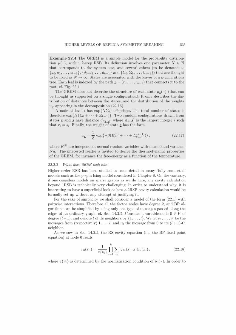
HIGHER LEVELS OF REPLICA SYMMETRY BREAKING 535
Example 22.4 The GREM is a simple model for the probability distribu-tion µ( · ), within k-step RSB. Its definition involves one parameter N ∈ N
that corresponds to the system size, and several others (to be denoted asa0, a1, . . . , ak−1, d0, d2, . . . , dk−1 and Σ0,Σ1, . . . ,Σk−1) that are thoughtto be fixed as N → ∞. States are associated with the leaves of a k-generationstree. Each leaf is indexed by the path r = (r0, . . . , rk−1) that connects it to theroot, cf. Fig. 22.4.
The GREM does not describe the structure of each state µr( · ) (that canbe thought as supported on a single configuration). It only describes the dis-tribution of distances between the states, and the distribution of the weightswr appearing in the decomposition (22.16).
A node at level i has expNΣi offsprings. The total number of states istherefore expN(Σ0 + · · · + Σk−1). Two random configurations drawn fromstates r and s have distance di(r,s), where i(r, s) is the largest integer i suchthat ri = si. Finally, the weight of state r has the form
wr =1
Zexp−β(E(0)
r0+ · · · + E(k−1)
rk−1) , (22.17)
where E(i)r are independent normal random variables with mean 0 and variance
Nai. The interested reader is invited to derive the thermodynamic propertiesof the GREM, for instance the free-energy as a function of the temperature.
22.2.2 What does 2RSB look like?
Higher order RSB has been studied in some detail in many ‘fully connected’models such as the p-spin Ising model considered in Chapter 8. On the contrary,if one considers models on sparse graphs as we do here, any cavity calculationbeyond 1RSB is technically very challenging. In order to understand why, it isinteresting to have a superficial look at how a 2RSB cavity calculation would beformally set up without any attempt at justifying it.
For the sake of simplicity we shall consider a model of the form (22.1) withpairwise interactions. Therefore all the factor nodes have degree 2, and BP al-gorithms can be simplified by using only one type of messages passed along theedges of an ordinary graph, cf. Sec. 14.2.5. Consider a variable node 0 ∈ V ofdegree (l+1), and denote l of its neighbors by 1, . . . , l. We let ν1, . . . , νl be themessages from (respectively) 1, . . . , l, and ν0 the message from 0 to its (l + 1)-thneighbor.
As we saw in Sec. 14.2.5, the RS cavity equation (i.e. the BP fixed pointequation) at node 0 reads
ν0(x0) =1
zνi
k∏
i=1
∑
xi
ψ0i(x0, xi)νi(xi) , (22.18)
where zνi is determined by the normalization condition of ν0( · ). In order to

536 AN ONGOING STORY
lighten the notation, it is convenient to introduce a function f0 that, evaluatedon l messages ν1, . . . , νl returns the message ν0 as above. We will therefore writeEq. (22.18) in shorthand form as ν0 = f0νi. Each νi is a point in the (|X |− 1)-dimensional simplex.
The 1RSB cavity equations are obtained from Eq. (22.18) by promoting themessages νi to random variables with distribution Qi( · ), cf. Ch. 19. The equa-tions depend on the 1RSB parameter (a real number), that we denote here asx1. Adopting a continuous notation for the messages distributions, we get
Q0(ν0) =1
ZQi
∫zνix1 δ(ν0 − f0νi)
l∏
i=1
dQi(νi) , (22.19)
Analogously to the replica-symmetric case, Eq. (22.18), we shall write Q0 =F0Qi as a shorthand for this equation. The function F0 takes as argument ldistributions Q1, . . . , Ql and evaluates a new distribution Q0 (each of the Qi’s isa distribution over the (|X |− 1)-dimensional simplex).
At this point the formal similarity of Eqs. (22.18) and (22.19) should beclear. The 2RSB cavity equations are obtained by promoting the distributionsQi to random variables (taking values in the set of distributions over the |X |-dimensional simplex)33. Their probability distributions are denoted as Qi, andthe resulting equations depend on one further real parameter x2. Formally the2RSB equation can be written as
Q0(Q0) =1
ZQi
∫ZQix2/x1 δ(Q0 − F0Qi)
l∏
i=1
dQi(Qi) . (22.20)
This equation might look scary, as Qi( · ) are distributions over distributions overa compact subset of the reals. It is useful to rewrite it in a mathematically morecorrect form. This is done by requiring, for any measurable set of distributionsA (see the footnote), the following equality to hold:
Q0(A) =1
ZQi
∫ZQix2/x1 I(F0Qi ∈ A)
l∏
i=1
dQi(Qi) . (22.21)
The interpretation of the 2RSB messages Qi is obtained by analogy with the1RSB one. Let α1 be the index of a particular cloud of states and Qα1
i ( · ) bethe distribution of the message νi over the lumps in cloud α1. Then Qi is thedistribution of Qα1
i when one picks up a cloud index α1 randomly (each cloudbeing sampled with a weight that depends on x1.)
33The mathematically inclined reader might be curious about the precise definition of aprobability distribution over the space of distributions. It turns out that given a measure spaceΩ (in our case the (|X |− 1) dimensional simplex), the set of distribution over Ω can be givena measurable structure that makes 2RSB equations well defined. This is done by using thesmallest σ-field under which the mapping Q "→ Q(A) is measurable for any A ⊆ Ω measurable.

HIGHER LEVELS OF REPLICA SYMMETRY BREAKING 537
In principle Eq. (22.20) can be studied numerically by generalizing the pop-ulation dynamics approach of Ch. 19. In the present case one can think of twoimplementations: for one given instance, one can generalize the SP algorithm,but this generalization involves, on each directed edge of the factor graph, a pop-ulation of populations. If instead one wants to perform a statistical analysis ofthese messages, seeking a fixed point of the corresponding density evolution, oneshould use a population of populations of populations! This is obviously chal-lenging from the point of view of computer resources (both memory and time).To the best of our knowledge it has been tried only once, in order to computethe ground state energy of the spin glass on random 5-regular graphs. Becausethe graph is regular it looks identical at any finite distance from any given point.One can therefore seek a solution such that the Qi on all edges are the same, andone is back to the study of populations of populations. The results have beensummarized in Table 17.4.5: if one looks at the ground state energy, the 2RSBmethod provides a small correction of order 10−4 to the 1RSB value, and thiscorrection seems to be in agreement with the numerical estimates of the groundstate.
22.2.3 Local stability of the 1RSB phase
The above discussion of 2RSB will help us to check the stability of the 1RSBphase. The starting point consists in understanding the various ways in whichthe 2RSB formalism can reduce to the 1RSB one.
The first obvious reduction consists in taking the 2RSB distribution Qi tobe a Dirac delta at Q∗
i . In other words, for any continuous functional F on thespace of distributions
∫F(Qi) dQi(Qi) = F(Q∗
i ) . (22.22)
It is not hard to check that, if Q∗i solves the 1RSB equation Eq. (22.19), this
choice of Qi solves Eq. (22.20) independently of x2.There exists however a second reduction, that corresponds to taking Qi( · )
a non-trivial distribution, but supported on Dirac deltas: let us denote by δν∗ a1RSB distribution which is a Dirac delta on the message ν = ν∗. Given a set ofmessagesQ∗
i that solves the 1RSB equation Eq. (22.19), we construct Qi( · ) asa superposition of Dirac deltas over all values of ν∗, each one appearing with aweight Q∗
i (ν∗). Again this distribution is more precisely defined by its action on
a continuous functional F(Q):
∫F(Qi) dQi(Qi) =
∫F(δν∗) dQ∗
i (ν∗) . (22.23)

538 AN ONGOING STORY
Exercise 22.2 Suppose that Q∗i solves the analog of the 1RSB equation
Eq. (22.19) in which the parameter x1 has been changed into x2. Show that Qi
defined by Eq. (22.23) solves Eq. (22.20) independently of x1.[Hint: Show that, when evaluated on Dirac deltas, the normalization Z
appearing in (22.19) is related to the normalization z in (22.18) by Zδνi =(zνi)x1 .]
In view of the interpretation of the 2RSB messages Qi outlined in the pre-vious section, and cartooned in Fig. 22.2.1, these two reductions correspond toqualitatively different limit situations. In the first case, described by Eq. (22.22),the distribution over clouds becomes degenerate: there is essentially one cloud(by this we mean that the number of clouds is not exponentially large in N : thecorresponding complexity vanishes). In the second case, described by Eq. (22.23),it is the distribution within each cloud that trivializes: there is only one cluster(in the same sense as above) in each cloud.
What are the implications of these remarks? Within the 1RSB approach oneneeds to solve Eq. (22.19) in the space of didtributions over BP messages: letus call this the ‘1RSB space’. When passing to 2RSB, one seeks a solution of(22.20) within a larger ‘2RSB space,’ namely the space of distributions overdistributions over BP messages. Equations (22.22) and (22.23) provide two waysfor embedding the 1RSB space inside the 2RSB space.
When one finds a 1RSB solution, one should naturally ask whether thereexists a proper 2RSB as well (i.e. a solution outside the 1RSB subspace). If thisis not the case, physicists usually conjecture that the 1RSB solution is asymp-totically correct (for instance it yields the correct free-energy per spin). Thischeck has been carried out for models on complete graph (e.g. the fully con-nected p-spin glasses). So far, the difficulty of studying the 2RSB equations haveprevented its implementation for sparse factor graph.
Luckily there is a convenient (albeit less ambitious) alternative: check thelocal stability of 1RSB solutions with respect to higher order RSB. Given a1RSB solution, one looks at it as a point in the 2RSB space according to the twopossible embeddings, and one studies the effect of a small perturbation. Moreprecisely, consider the iteration of 2RSB equations (22.20):
Q(t+1)i→j (Q0) =
1
ZQl→i
∫ZQl→ir δ(Qi→j − FiQl→i)
∏
l∈∂i\j
dQ(t)l→i(Ql→i) .
Given the factor graph G, we initiate this iteration from a point close to the 1RSBsolution described by either of the embeddings (22.22) or (22.23) and see if, theiteration converges back to the 1RSB fixed point. This is studied by linearizingthe iteration in an appropriate ‘perturbation’ parameter. If the iteration doesnot converge to the 1RSB fixed point, the 1RSB solution is said unstable. Theinstability is named of ‘type I’ if it occurs when embedding (22.22) is used andnamed of ‘type II’ for embedding (22.23).

HIGHER LEVELS OF REPLICA SYMMETRY BREAKING 539
Fig. 22.5. Cartoon of the two types of local instabilities from a 1RSB solutiontowards 2RSB.
An alternative approach for checking the local stability of a 1RSB solutionconsists in computing the spin glass susceptibility, which describes the reactionof the model (22.16) to a perturbation that acts on a single variable xi. Aswe discussed above, the effect of this perturbation (studied in linear order) re-mains finite when the spin glass susceptibility χ(2) is finite. One should thereforecompute χ(2) assuming that the 1RSB solution is correct and check that it isfinite. However, the 1RSB picture implies a second condition: each single lump rshould also be stable to small perturbations. More precisely, we define χSG,r asthe spin glass susceptibility with respect to the measure µr( · ) restricted to stater. Denoting by 〈 · 〉r the expectation value with respect to µr, the ‘intra-state’susceptibility, χSG,intra, is a weighted average of χSG,r over the state r:
χSG,intra =∑
r
wr χSG,r, (22.24)
χSG,r =1
N
∑
i,j
(〈xixj〉r − 〈xi〉r〈xj〉r
)2. (22.25)
Within the susceptibility approach, the second condition consists in computingχSG,intra with the 1RSB approach and requiring that it stays finite as N →∞.
It is generally believed that these two approaches to the local stability ofthe 1RSB phase coincide. Type I stability should be equivalent to χ(2) beingfinite; it means that the system is stable with respect to the grouping of statesinto clusters. Type II stability should be equivalent to χSG,intra being finite; itmeans that the system is stable towards a splitting of the states into sub-states.A pictorial representation of the nature of the two instabilities in the spirit ofFig. 22.2.1 is shown in Fig. 22.2.3.
The two approaches to stability computations have been developed in severalspecial cases, and are conjectured to coincide in general. Remarkably 1RSB is

540 AN ONGOING STORY
Σe
e
1RSB stable region
d m Gs
d(α)G(α)(α)s
α α α0
0.002
0.004
0.006
0.010
0.012
0.014
3.9 4 4.1 4.2 4.3 4.4 4.5 4.6
ener
gy
α−0.002
0.008
α
ee
e
Fig. 22.6. Top: The energetic complexity Σe in a random 3-SAT problem, com-puted within the 1RSB cavity method, is plotted versus the density e ofviolated clauses, for α = 4.1, 4.2, and 4.3 (from top to bottom). The curvereproduces Fig. 20.5, but it now shows the stable and unstable regions. Thefull thick line, below eG(α), gives the part of the complexity curve for whichthe 1RSB computation is locally stable (absent for α = 4.1 < αm(3), wherethe full curve is unstable). This is the only part that is computed reliablyby 1RSB, the dashed part is unstable. Bottom: In the same random 3-SATproblem, plotted versus the clause density α: the continuous line gives theminimum density of unsatisfied clauses as predicted within 1RSB (this is thevalue of e where Σe(e) starts to become positive). The dotted line gives thethreshold energy density as predicted within 1RSB (the maximal value of ewhere Σe(e) exists). The gray area indicates the region of local stability of the1RSB stability. The ground state energy density predicted by 1RSB is wrongfor α > αG (although probably very close to the actual value), because inthis region there is an instability towards higher order RSB. It is conjecturedthat the stable region, αm < α < αs, is in a 1RSB phase: if this conjectureholds the 1RSB prediction αs for the SAT-UNSAT threshold is correct. ForK = 3 one has αm(3) = 4.153(1), αs(3) = 4.2667(1), αG(3) = 4.390(5).

HIGHER LEVELS OF REPLICA SYMMETRY BREAKING 541
unstable in several interesting cases and higher order RSB would be needed toobtain exact predictions.
Stability computations are somewhat involved, and a detailed description isbeyond our scope. Nevertheless, we want to give an example of the results thatcan be obtained through a local stability analysis. Consider random K-SATformulae, with N variables and M = Nα clauses. Let es(α) denote the minimumnumber of unsatisfied clauses per variable, in the large system limit. The limites(α) can be computed along the lines of Ch. 20 using the 1RSB cavity method:for a given α, one computes the energetic complexity density Σe(e) versus thedensity of violated clauses e. Then es(α) is found as the minimal value of u suchthat Σe(e) > 0. It vanishes for α < αs(K) (the SAT-UNSAT threshold) anddeparts continuously from 0, increasing monotonically for α > αs(K).
The stability computation shows that, for a given α, there is in general aninstability of type II which appears above some value e = eG(α): only the partof Σe(e) with e ≤ eG(α) is in a locally stable 1RSB phase. When α < αm(K),eG(α) = 0 and the whole 1RSB computation is unstable. For α > αG(K),eG(α) < es(α) (the ground state energy density) and again 1RSB is unstable (thisimplies that the 1RSB prediction for es(α) is not correct). The conclusion is thatthe 1RSB calculation is stable only in an interval ]αm(K),αG(K)[. Figure 22.2.3summarizes this discussion for 3-SAT. For all values of K, the stable interval]αm(K),αG(K)[ contains the SAT-UNSAT threshold αs(K).
The stability check leads to the conjecture that the 1RSB prediction forαs(K) is exact. Let us stress however that stability has been checked only withrespect to small perturbations. A much stronger argument would be obtained ifone could do the 2RSB computation and show that it has no solution apart fromthe two ‘embedded 1RSB solutions’ that we discussed above.
22.2.4 Open problems within the cavity method
The main open problem is of course to prove that the 1RSB cavity approachyields correct predictions in some models. This was achieved until now only fora class of models on the complete graph. Here we want to point out a numberof open questions that wait for an answer, even at a heuristic level, within the1RSB cavity method itself.
Distributional equations. Cavity predictions are expressed in terms of fixedpoint of equations of the form (22.19). When considering models on ensembles ofrandom graphs, this can be read as an equation for the probability distributionof Q0( · ) (that is taken identical to the one of Q1( · ),. . . , Qk( · ).)
Currently such equations are mostly studied using the population dynamicsmethod of Sec. 14.6.4. The main alternative explored so far has been to formallyexpand the equations for large degrees. Population dynamics is powerful andversatile. However in many cases, this approach is too coarse, particularly assoon as one wants to study k-RSB with k ≥ 2. It is intrinsically hampered bystatistical errors, that are of the order of the inverse square root of populationsize. In some models (for instance, in graph ensembles with large but bounded

542 AN ONGOING STORY
average degree), statistical fluctuations are too large for the population sizes thatcan be implemented on ordinary PCs (typically 107 ÷ 108 elements). This limitsthe possibility to distinguish, for instance, 2RSB from 1RSB effects, because highprecision is generally required to see the difference. Furthermore, metastability isthe crux (and the limit) of the whole population dynamics approach. Thereforeit would be interesting to make progress in two directions:
• Analytical tools and generic results on the cavity equations; this couldprovide important guiding principles for any numerical study.
• New efficient and stable numerical methods.
A step forward has been made by the reconstruction algorithm discussed in The-orem 19.5, but unfortunately it is limited to one value of the rescaling parameter,x = 1.
Local stability. Local stability criteria provide an important guidance in heuris-tic studies. It would be important to put these results on firmer grounds. Twospecific tasks could be, for instance:
• Prove that, if all 1RSB solutions of the cavity equations are locally unsta-ble, then there must exist a 2RSB solution outside the 1RSB subspace.
• Prove that, if a solution of the cavity equations is locally unstable, it doesnot describe correctly the model.
Occurrence of k-RSB. A number of random graphical models have been stud-ied within the cavity (or replica) method. In most cases, one finds that the systemis either RS, or 1RSB, or FRSB. The cases in which a 2RSB phase is found arerare, and they always involve some kind of special construction of the compati-bility function (for instance, a fully connected model which is a superposition oftwo p-spin glass interactions, with p1 = 3 and p2 = 16 displays 2RSB). Thereforeone should
• Find a ‘natural’ model for which 2RSB is asymptotically exact, or under-stand why this is impossible.
Full replica-symmetry breaking. We saw that k-RSB provides, as k increases,a sequence of ‘nested’ schemes that aim at computing various quantities like localmarginals, free-entropy density, etc. . . , in the large system limit. A k-th orderscheme includes all the lower l-RSB schemes with l < k as nested subspaces ofthe set of feasible solutions to the cavity equations. On the other hand, as thenumber of steps increases, the description of the set of feasible solutions becomesmore and more complicated (distributions of distributions of. . . ).
Surprisingly, in the case of fully connected models, there exists a compactdescription of the space of feasible solutions in the FRSB limit k → ∞. Anoutstanding problem is to find an analogous description in the case of models onsparse graphs. This would allow to look for the best solution in the k-RSB spacefor all k.

PHASE STRUCTURE AND THE BEHAVIOR OF ALGORITHMS 543
• Find a description of the space of full replica-symmetry breaking messagesfor models on sparse graphs.
Variational aspect. It is widely believed that if one finds a consistent solution ofthe cavity k-RSB equations, the free-energy density computed with this solution,is always a lower bound to the correct free energy density of the model (inparticular the k-RSB ground state energy density prediction is a lower boundto the true one). This should hold for a large class of models with a statistical+1/− 1 symmetry. While this has been proven in some specific cases, one wouldlike to:
• Find a general proof that the free-energy computed with the cavity methodis a lower bound to the correct free-energy of the model.
22.3 Phase structure and the behavior of algorithms
A good part of this book has been devoted to the connection between the variousphases in random graphical models, and the behavior of algorithms. There existsby now substantial evidence (empirical, heuristic, and, in some cases, rigorous)that such a connection exists. For instance, we have seen on the example of codesin Ch.21 how the appearance of a 1RSB phase, and the corresponding prolifer-ation of metastable states, determines the noise threshold where BP decodingfails. Developing a broader understanding of this connection, and determiningthe class of algorithms to which it applies, is a very important problem.
We propose here a list of broad research problems, whose advancement willprobably help to clarify this issue. We always have in mind a graphical model ofthe form (22.1), with a locally tree-like factor graph.
Impact of the dynamical transition on Monte Carlo dynamics.Consider the problem of sampling from the distribution (22.1) using a Monte
Carlo Markov Chain (MCMC) algorithm. The Markov chain is assumed to flipa sub-linear (o(N)) number of variables at each step, and to satisfy detailedbalance with respect to the probability distribution µ( · ).
One expects that, if the system is in a 1RSB phase, the relaxation time ofthis algorithm will increase rapidly (probably exponentially) with system size.Intuitive arguments in favor of this statement can be obtained from each of thetwo characterizations of the 1RSB phases introduced in Sec. 22.1. The argumentis different whether we start from the pure state decomposition, or from thecharacterization in terms of correlations. In the first case, the relaxation time isestimated through the time to cross a bottleneck, see also Ch. 13. In the secondcase, one can define a correlation length -∗i through the point-to-set correlationfunction Gi(-), cf. Eq. (22.14). In order for the system to relax, information hasto travel a distance -∗i . But if -∗i diverges with size, so must the relaxation time.
This picture is intuitively satisfying, but it is far from being proved, andshould be formulated more precisely. For instance it often happens that in RSphases there exist small isolated metastable states that make the relaxation time(the inverse spectral gap of the MCMC) formally large. But even in such cases,

544 AN ONGOING STORY
numerical simulations indicate that Glauber dynamics equilibrates rapidly withinthe RS phase. This observation is probably related to the fact that the initialcondition is chosen uniformly random, and that equilibration is only checked onlocal observables. A number of questions arise:
• Why is metastability irrelevant ‘in practice’ in a RS phase? Is it becauseof local measurements? Or because of the uniform initial condition? If thelatter is true, what is so special about the uniform initial condition?
• Within a RS phase, can one approximate partition functions efficiently?
Message passing and the estimation of marginals.For a number of models on sparse random graphs within the RS and (some-
times) dynamical 1RSB phases, message passing methods like belief propagationor survey propagation show, empirically, good performances. More precisely, theyreturn good approximations of local expectation values if initialized from uniformmessages.
Current rigorous techniques for analyzing BP often aim at proving that it isaccurate regardless of the initialization. As a consequence, results are dominatedby the behavior under worst case initializations that are not used in practice.As an illustration, consider applying BP to the uniform measure over solutionsof a random K-SAT formula. The analysis under worst case initialization allowsto prove that BP is accurate only for α ≤ (2 log K)/K[1 + o(1)]. This thresholdis embarrassingly small when compared to the dynamical transition point thatterminates the RS phase αd(K) = 2K log K/K[1 + o(1)].
In general we have no good mathematical control of when BP or SP convergeor/and give good approximations of marginals. Empirically it seems that SP isable to converge in some regions of 1RSB phases where BP does not. We haveno real understanding of this fact beyond the hand-waving argument that 1RSBcorrectly captures the structure of correlations in these phases.
Here are a number of open questions on these issues:
• Why are BP/SP performances on random instances, with uniformly ran-dom initialization, much better than in the worst case? What is specialabout the uniform initialization? What are the features of random instancesthat make them easier? Can these features be characterized and checkedefficiently?
• Under what conditions do the BP (or the SP) algorithms converge and givegood approximations to local marginals? When their naive iteration doesnot converge, can one systematically either force convergence or use timeaverages of the messages?
• It seems that, on sparse random graphical models, BP or SP outperformslocal MCMC algorithms. In particular these message passing algorithmscan have (at least in principle), good performances within the dynamical1RSB phase. Can one demonstrate this possibility convincingly in somemodel?

PHASE STRUCTURE AND THE BEHAVIOR OF ALGORITHMS 545
Message passing algorithms and optimization.If one seeks a solution to a random constraint satisfaction problem using
message passing, the main approach so far has been the use of decimation: onefirst computes all local marginals, then decides, based on this knowledge, how tofix a variable, and then iterate the procedure. In general this procedure convergeswhen the number of constraints per variable is not too large, but it fails abovea critical value of this number, which is strictly smaller than the SAT-UNSATthreshold. No one knows how to determine analytically this threshold.
An alternative to decimation is the reinforcement method: instead of fixinga variable based on the knowledge of local marginals, it modifies some localfactors applying to each individual variables, based on this same information. Sofar, optimizing this modification is an art, and its critical threshold cannot beestimated either.
• How to predict the performances of BP+ decimation or SP+decimation.For instance, empirically these methods find solutions to random K-SATformulae with high probability for α < αBP(K) (or α < αSP(K)), butwe have no prediction for these algorithmic thresholds. In what class ofproblems is SP better than BP?
• Similar questions for BP+reinforcement or SP+reinforcement.
• Find new ways to use the local marginal information found by messagepassing in order to exhibit solutions.
• In an UNSAT phase, the message passing procedure is able to give anestimate of the minimal number of violated constraints. Is it possible touse this information, and the one contained in the messages, in order toprove unsatisfiability for one given instance?
The above questions focus on sparse random instances. Message passing tech-niques have been (partially) understood and sharpened for this type of instances.They naturally arise in a large class of applications where the graphical modelis random, or pseudo-random, by design. The theory of sparse graph codes is aclear example in this direction. In the limit of large block-lengths, random con-structions proved to be generally superior to deterministic ones. More recentlysparse graph constructions have been proposed for data compression (both loss-less and lossy), online network measurements, multi-terminal communications,distributed storage, group testing, etc. . .
On the other hand, being able to deal with structured graphs would open aneven much broader class of applications. When applied to structured problems,message passing algorithms often fail to converge. This is typically the reason whythe decimation method may fail, even when the marginals of the original problemare well estimated by message passing: the instance found after fixing manyvariables is no longer random. Finding appropriate modifications of messagepassing for structured graphs would therefore be very interesting.

546 AN ONGOING STORY
• How to use message passing in order to improve the solution of some generalclasses of (non-random) constraint satisfaction problems. Can it be coupledefficiently to other general methods (such as MCMC)?
Notes
The present chapter was inevitably elliptic. We will provide a few pointers torecent research without any ambition to be comprehensive.
The connection between correlation lengths and phase transitions is a classicaltopic in statistical mechanics which has been recently revived by the interest inthe glass transition. A good starting point for learning about this subject in thecontext of glasses is the paper (Bouchaud and Biroli, 2004) which describes the‘freezing’ thought experiment in Sec. 22.1.2.
The description of point-to-set correlations in terms of ‘reconstruction’ prob-lems is taken from (Evans, Kenyon, Peres and Schulman, 2000). This paperstudies the reconstruction phase transition for Ising models on trees. Results fora wide class of models on trees are surveyed in (Mossel and Peres, 2003; Mossel,2004). We also refer to (Gerschenfeld and Montanari, 2007) for the generaliza-tion to non-tree graphs. The connection between ‘reconstruction’ and ‘dynamical’1RSB phase transition was first pointed out in (Mezard and Montanari, 2006).The implications of this phase transition on dynamics were explored in (Berger,Kenyon, Mossel and Peres, 2005; Martinelli, Sinclair and Weitz, 2004; Montanariand Semerjian, 2006b). The definition of pure states presented in this chapteras well as the location of the dynamical and condensation phase transitions forrandom K-SAT and coloring of random graphs are from (Krzakala, Montanari,Ricci-Tersenghi, Semerjian and Zdeborova, 2007).
The GREM has been introduced by (Derrida, 1985) and studied in detailsin (Derrida and Gardner, 1986). A 2RSB phase in fully connected models hasbeen found by (Crisanti and Leuzzi, 2007). There are very few results abouthigher order RSB in models on sparse random graphs. For spin glasses, onecan use perturbative expansions close to the critical point (Viana and Bray,1985), or for large degrees (Goldschmidt and Dominicis, 1990). The 2RSB com-putation of ground state energy for spin glasses mentioned in Sec. 22.2 is from(Montanari, 2003). The method for verifying the local stability of the 1RSB so-lution in sparse systems was first devised in (Montanari and Ricci-Tersenghi,2003), and applied to random satisfiability problems in (Montanari, Parisi andRicci-Tersenghi, 2004). A complete list of stability thresholds, including theirasymptotic behavior, for random K-SAT can be found in (Mertens, Mezard andZecchina, 2006). The interpretation of 1RSB instability in terms of susceptibili-ties is discussed in (Rivoire, Biroli, Martin and Mezard, 2003).
The fact that the free-energy computed with the cavity (or replica) method isa lower bound to the true one can be proven in some fully connected models usingthe inequalities of (Guerra, 2003). The same strategy also yields rigorous boundsin some diluted systems (Franz and Leone, 2003; Franz, Leone and Toninelli,

NOTES 547
2003; Panchenko and Talagrand, 2004) but it still relies on some details of thestructure of the models, and a general proof applicable to all cases is lacking.
The reinforcement algorithm has been introduced and discussed for SAT in(Chavas, Furtlehner, Mezard and Zecchina, 2005).
There exist only scarce results on the algorithmic consequences of the struc-ture of the solution space. Some recent analyses can be found in (Altarelli,Monasson and Zamponi, 2007; Montanari, Ricci-Tersenghi and Semerjian, 2007;Ardelius and Aurell, 2006; Alava, Ardelius, Aurell, Kaski, Krishnamurthy, Or-ponen and Seitz, 2007). The convergence and correctness of BP for randomK-satisfiability at small enough α was proven in (Montanari and Shah, 2007).
This book covered only a small subsets of problems that lie at the intersectionbetween information theory, computer science and statistical physics. It wouldbe difficult to provide an exhaustive list of references on the topics we did nottouch: we will limit ourselves to a few ‘access points’.
As we mentioned, channel coding is only one of the fundamental problemsaddressed by information theory. Data compression, in particular in its ‘lossy’version, is a key component in many modern technologies, and presents a num-ber of open problems (Ciliberti, Mezard and Zecchina, 2005; Wainwright andManeva, 2005). Some other statistics problems like group testing are similar inspirit to data compression (Mezard, Tarzia and Toninelli, 2007).
Modern wireless and wireline communication systems are intrisically multi-user systems. Finding optimal coding schemes in a multiuser context is a widelyopen subject of great practical interest. Even the information theoretic capacityof such systems is unknown. Two fields that benefited from tools or analogieswith statistical mechanics are multiuser detection (Tanaka, 2002; Guo and Verdu,2002) and networking (Kelly, 1991). Always within a communications context,a large effort has been devoted to characterizing large communication networkssuch as the Internet. A useful review is provided by (Kleinberg, Kumar, Ragha-van, Rajagopalan and Tomkins, 1999).
Statistical mechanics concepts have been applied to the analysis of fluctu-ations in financial markets (Bouchaud and Potters, 2003) or to model interac-tions among economic agents (Challet, Marsili and Zhang, 2005). Finally, biol-ogy presents a number of problems in which randomness, interaction betweendifferent components, and robustness play important roles. Stochastic models onnetworks, and inference algorithms have been studied in a number of contexts,from neural networks (Baldassi, Braunstein, Brunel and Zecchina, 2007; Coolen,Kuehn and Sollich, 2005) to phylogeny (Mossel, 2003), to gene expression (Fried-man, Linial, Nachman and Peer, 2000).
A few of these topics, and others, are reviewed in the recent school proceedings(Bouchaud, Mezard and Dalibard, 2007).