linear b-spline copulas with applications to nonparametric estimation of copulas

Computational Statistics and Data Analysis 52 (2008) 3806–3819www.elsevier.com/locate/csda

Linear B-spline copulas with applications to nonparametricestimation of copulas

Xiaojing Shena, Yunmin Zhua,∗, Lixin Songb

a Department of Mathematics/Key Lab of Fundamental Science for National Defense, Sichuan University, Chengdu, 610064, PR Chinab Department of Applied Mathematics, Dalian University of Technology, Dalian, 116024, PR China

Received 19 December 2006; received in revised form 5 January 2008; accepted 7 January 2008Available online 16 January 2008

Abstract

In this paper, we propose a method for constructing a new class of copulas. They are called linear B-spline copulas whichare a good approximation of a given complicated copula by using finite numbers of values of this copula without the loss ofsome essential properties. Moreover, rigorous analysis shows that the empirical linear B-spline copulas are more effective thanempirical copulas to estimate perfectly dependent copulas. For the cases of nonperfectly dependent copulas, simulations show thatthe empirical linear B-spline copulas also improve the empirical copulas to estimate the underlying copula structure. Furthermore,we compare the performance of parametric estimation of copulas based on the empirical copulas with that based on the empiricallinear B-spline copulas by simulations. In most of the cases, the latter are better than the former.c© 2008 Elsevier B.V. All rights reserved.

1. Introduction

Copulas have recently been a hot topic in finance and insurance, since they represent a methodology whichis important to handle in a flexible way the dependence between market risk factors and other relevant variables(see Embrechts et al. (2002)). The importance of copulas in modelling is justified by the well-known Sklar’s(1959) theorem: if H(x1, x2, . . . , x p) on R p is a p-dimensional joint distribution function with marginal distributionfunctions F1(x1), F2(x2), . . . , Fp(x p), then there exists an unique copula function C(u1, u2, . . . , u p) in the rangeof (F1, F2, . . . , Fp) such that H(x1, x2, . . . , x p) = C(F1(x1), F2(x2), . . . , Fp(x p)). Sklar’s theorem shows that oneadvantage of copulas is to separate out the dependence from the marginal behavior of relevant random variables.Consequently, copulas allow one to estimate the dependence structure of relevant random variables and marginaldistributions separately.

For the estimation of copulas, there are parametric and nonparametric approaches. If the true copula belongs to anassumed parametric family, the maximum likelihood methods are of interest and the estimated copula is good fit todata. These methods are detailed in Genest et al. (1995) and Joe and Xu (1996). Kim et al. (2007) proposed an elaboratecomparison of them. If the true copula, however, is out of the assumed parametric family, the parametric approach

∗ Corresponding author. Tel.: +86 028 85415070.E-mail address: [email protected] (Y. Zhu).

0167-9473/$ - see front matter c© 2008 Elsevier B.V. All rights reserved.doi:10.1016/j.csda.2008.01.002

http://www.elsevier.com/locate/csda

mailto:[email protected]

http://dx.doi.org/10.1016/j.csda.2008.01.002

X. Shen et al. / Computational Statistics and Data Analysis 52 (2008) 3806–3819 3807

usually leads to a poor fit to data. The alternative approach is nonparametric estimation of copulas. Deheuvels (1979)presented a nonparametric method called empirical copulas. They converge uniformly to the underlying copula andare also used to construct nonparametric tests for independence. In addition, Deheuvels (1981a,b) established the weakconvergence of the empirical copula process in the case of independent marginal distributions. The weak convergenceof the empirical copula process in Skorokhod space D([0, 1]

2) was also considered by Gaenssler and Stute (1987).Van der Vaart and Wellner (1996) proved the weak convergence of the empirical copula process in l∞([u, v]

2), forsome 0 < u < v < 1. Fermanian et al. (2004) presented the weak convergence of this process in l∞([0, 1]

2) underweaker assumptions. The discussion for time series can be found in Fermanian and Scaillet (2003).

In this paper, based on the linear B-spline, we propose a method of constructing a new class of copulas which arecalled linear B-spline copulas. Then, we provide necessary and sufficient conditions for this method to yield a copula.The properties of the linear B-spline copulas are presented. The advantage of the method is that a complicated copulacan be uniformly approximated by the linear B-spline copulas without loss of some essential properties. In addition,part of our motivation for studying the nonparametric estimation of copulas is to hope that a new nonparametricestimation based on both the linear B-spline copulas and the empirical copulas has richer properties than the empiricalcopulas. As we shall see in the following sections, indeed, the new nonparametric estimation can overcome thediscontinuous of the empirical copulas so that the concept positively quadrant dependent (PQD) can be empiricallyanalyzed and it is helpful to find a parametric family of copulas by the way of graph comparison processing on samples(see Embrechts et al. (2002)). Based on theoretical analysis and simulations, we find that the new method can improvethe estimation performance in comparison with the empirical copulas. Moreover, we extend the parametric estimationmethod of copulas proposed by Durrleman et al. (2000).

The paper is organized as follows. In Section 2, we briefly review the copulas and linear B-spline approximation.In Section 3, we present linear B-spline copulas and their properties. In Section 4, empirical linear B-spline copulasare proposed and their estimation performance for perfectly dependent copulas is analyzed, and their asymptoticproperties are also given. In Section 5, comparison of nonparametric estimation and that of parametric estimationbased on the empirical copulas and the empirical linear B-spline copulas are given by simulations. In Section 6, wepresent the conclusion and discussion. Main proofs are gathered in the Appendix.

2. Preliminaries

2.1. The Copula functions

We review some basic concepts and properties of copulas by referring to the recent book of Nelsen (1999) (or(Joe, 1997; Cherubini et al., 2004)). For simplicity, let us consider the bivariate case. A bivariate copula is a functionC : I 2

→ I = [0, 1] such that:

1. C(x, 0) = C(0, y) = 0, for every x, y ∈ I. (1)

2. C(x, 1) = x, C(1, y) = y, for every x, y ∈ I. (2)

3. C is 2-increasing, i.e., for every rectangle [x1, x2]×[y1, y2] in I 2, the associated C-volume VC ([x1, x2]×[y1, y2])

satisfies

VC ([x1, x2] × [y1, y2]) = C(x1, y1) − C(x1, y2) − C(x2, y1) + C(x2, y2) ≥ 0. (3)

In fact, copula is a joint distribution whose marginal distributions are uniform distributions on the interval I .If C is a copula, then for every (x, y) ∈ I 2, max(0, x + y − 1) ≤ C(x, y) ≤ min(x, y), the bounds are called

Frechet–Hoeffding bounds denoted by M(x, y) = min(x, y) and W (x, y) = max(0, x + y − 1), which are alsocopulas. We will say that random variables X and Y, with associated copula M (or W ), are perfectly positively (ornegatively) dependent. Moreover, if X and Y are continuous random variables, then Y is almost surely an increasing(or decreasing) function of X if and only if the copula of X and Y is M (or W ) (see Nelsen (1999), 6–27).

Nelsen (1993) has shown that radial and joint symmetry are essential properties of the copula associated with(X, Y ). Suppose that (X, Y ), with associated copula C , is marginally symmetric about (a, b). Then (X, Y ) is radiallysymmetric about (a, b) if and only if C satisfies

C(x, y) = x + y − 1 + C(1 − x, 1 − y); (4)

3808 X. Shen et al. / Computational Statistics and Data Analysis 52 (2008) 3806–3819

and (X, Y ) is jointly symmetric about (a, b) if and only if C satisfies

C(x, y) = x − C(x, 1 − y) and C(x, y) = y − C(1 − x, y). (5)

Besides, a copula C is symmetric if C(x, y) = C(y, x) for all (x, y) in [0, 1]2.

It is shown that for functions f and g, almost surely increasing on the same ranges as X and Y, CXY = C f (X)g(Y )

(see Schweizer and Wolff (1981)). Therefore, the nonparametric properties of the copula are invariant, which impliesthat the dependence measures can be expressed in terms of the copula and are invariant for increasing transformations.In fact, measures of dependence on copulas are more general than the linear correlation measure. The followingmeasures of dependence — Spearman’s rho, Gini’s gamma and Blomqvist’s beta can be found in Nelsen (1999):

ρC = 12∫ 1

0

∫ 1

0C(x, y)dxdy − 3,

γC = 4

[∫ 1

0C(x, 1 − x)dx −

∫ 1

0(x − C(x, x))dx

],

βC = 4C

(12,

12

)− 1.

The concept of PQD is due to Lehmann (1966). Let two random variables X1 and X2 are PQD if for all (x1, x2) inR2,

P(X1 ≤ x1, X2 ≤ x2) ≥ P(X1 ≤ x1)P(X2 ≤ x2). (6)

This shows that X1 and X2 are PQD if the probability that they are simultaneously small is at least as great as it wouldbe if they are independent. Moreover, if X1 and X2 are associated with copula C , then Condition (6) is equivalent toC(x, y) ≥ Π (x, y) = xy, x, y ∈ I . The importance of PQD has been emphasized in recent papers (see, Dhaene andGoovaerts (1996) and Embrechts et al. (2002)). Some nonparametric ways to test for PQD can be seen in Denuit andScaillet (2004) and Scaillet (2005). In addition, if X1 and X2 are PQD, we also say that their copula C is PQD.

We now recap the notion of empirical copulas. Let {(X i , Yi )}ni=1 denote a sample of size n from a continuous

bivariate distribution. The empirical copula is the function CE (x, y) given by

CE (x, y) =

CE

(i − 1

n,

j − 1n

),

i − 1n

≤ x <i

n,

j − 1n

≤ y <j

n,

1, x = y = 1,

(7)

where CE

(in ,

jn

)=

1n

∑nk=1 I{Xk≤X(i),Yk≤Y( j)}, CE (0, i

n ) = CE (jn , 0) = 0, i, j = 1, 2, . . . n, CE (0, 0) = 0, and X(k)

is the kth order statistic of the sample.

2.2. Linear B-spline approximation

In this subsection, we give the linear B-spline basis functions and deduce linear B-spline approximation. The B-spline was first proposed by Schoenberg and further amplified in his 1966 paper with Curry (see Curry and Schoenberg(1966)). The full and clear definition can be seen in de Boor (1978) or (Nurnberger, 1989).

Let knots vector (t0, t1, . . . , tn+2) be t0 = 0, ti =i−1

n , i = 1, . . . n, tn+1 = tn+2 = 1. We can obtain correspondinglinear B-spline basis functions as follows, for i = 1, . . . , n − 1,

Ni (x) =

nx − (i − 1),

i − 1n

≤ x <i

n,

(i + 1) − nx,i

n≤ x <

i + 1n

,

0, otherwise,

(8)

N0(x) =

{1 − nx, 0 ≤ x <

1n,

0, otherwise,(9)


Nn(x) =

{nx − (n − 1),

n − 1n

< x ≤ 1,

0, otherwise.(10)

The linear B-spline basis functions have the following properties, for i = 1, . . . , n,

Ni (x)

{≥ 0,

i − 1n

≤ x <i + 1

n,

= 0, otherwise,(11)

n∑i=0

Ni (x) = 1, 0 ≤ x ≤ 1, (12)

n∑i=0

i

nNi (x) = x, 0 ≤ x ≤ 1, (13)

where the first two properties (11) and (12) can be seen in de Boor (1978) or Nurnberger (1989); and the third Property(13) is because, for 0 ≤

kn ≤ x ≤

k+1n ≤ 1,

n∑i=0

i

nNi (x) =

k

nNk(x) +

k + 1n

Nk+1(x) =k

n[(k + 1) − nx] +

k + 1n

(nx − k) = x .

It can be shown that the linear B-splines form a basis of a spline space (see Nurnberger (1989)). They have smallestpossible support, in other words, they are zero on a large set. Therefore, the multiple correlation among them is smallerthan others and the linear B-splines basis, usually, is numerically more stable. In addition, a bivariate tensor productapproximation of f (x, y) in C[0,1]2 (C[0,1]2 is the space of continuous bounded functions on [0, 1]

2) is defined as

f (x, y) =

n∑i=0

n∑j=0

f

(i

n,

j

n

)Ni (x)N j (y). (14)

By the definition of the linear B-splines and their properties, we see that f (x, y) defined by Eq. (14) uniformlyapproximates f (x, y).

Lemma 1. Let f (x, y) be in C[0,1]2 . Then

supx,y∈I

| f (x, y) − f (x, y) |→ 0, n → ∞,

where f (x, y) is given in Eq. (14).

3. Linear B-spline copulas

From the linear B-spline approximation of Eq. (14), we can similarly define a map CLB : I 2→ I ,

CLB(x, y) =

n∑i=0

n∑j=0

θ

(i

n,

j

n

)Ni (x)N j (y). (15)

Under Conditions (16) and (17) below, CLB is the so-called linear B-spline copula.

Theorem 2. CLB(x, y) defined by Eq. (15) is a copula if and only if for 0 ≤ i, j ≤ n,

θ

(0,

j

n

)= θ

(i

n, 0

)= 0, θ

(i

n, 1

)=

i

n, θ

(1,

j

n

)=

j

n, (16)

and for 0 ≤ i, j ≤ n − 1,

θ

(i

n,

j

n

)− θ

(i + 1

n,

j

n

)− θ

(i

n,

j + 1n

)+ θ

(i + 1

n,

j + 1n

)≥ 0. (17)


In particular, if C is a copula and θ(

in ,

jn

)= C

(in ,

jn

), then CLB is a copula and uniformly approximates C .

From Eq. (13), it is easy to see that the independent copula is a special linear B-spline copula.

Theorem 3. If θ(

in ,

jn

)=

in ·

jn , 0 ≤ i, j ≤ n, then

CLB(x, y) = xy.

Moreover, if θ(

in ,

jn

)≥

in ·

jn , then CLB is PQD.

This theorem also shows that if C is PQD and θ(

in ,

jn

)= C

(in ,

jn

), then CLB is also PQD and uniformly

approximates C . The next theorem provides the bounds of the linear B-spline copulas for a fixed n.

Theorem 4. If θ(

in ,

jn

)= min

(in ,

jn

), 0 ≤ i, j ≤ n, then

CuLB(x, y) , CLB(x, y) =

k

n+ n

(x −

k

n

) (y −

k

n

),

k

n< x, y <

k + 1n

,

0 ≤ k ≤ n − 1,

min(x, y), otherwise.

If θ(

in ,

jn

)= max(0, i

n +jn − 1), 0 ≤ i, j ≤ n, then

C lLB(x, y) , CLB(x, y) =

n

(x −

k

n

) (y −

n − k − 1n

),

k

n< x, 1 − y <

k + 1n

,

0 ≤ k ≤ n − 1,

max(0, x + y − 1), otherwise.

Moreover, if CLB(x, y) is a copula, then

C lLB(x, y) ≤ CLB(x, y) ≤ Cu

LB(x, y).

Remark. This theorem gives the copulas CuLB(x, y) and C l

LB(x, y), which uniformly approximate Frechet–Hoeffdingupper bound (M) and Frechet–Hoeffding lower bound (W) respectively. Moreover, this theorem also shows that theycan be called Frechet–Hoeffding bounds of the linear B-spline copulas. The performance of Cu

LB(x, y) (or C lLB(x, y))

approximation to M (or W ) is assessed by its Integrated Absolute Error (IAE). The forms of the two (IAE)s are givenby

IAE(CuLB) =

∫ 1

0

∫ 1

0|M(x, y) − Cu

LB(x, y)|dxdy

=

n−1∑k=0

∫ k+1n

kn

∫ k+1n

kn

(min(x, y) − CuLB(x, y))dxdy

=

n−1∑k=0

∫ k+1n

kn

∫ k+1n

kn

(min(x, y) −

k

n− n

(x −

k

n

) (y −

k

n

))dxdy

=1

12n2 ,

IAE(C lLB) =

∫ 1

0

∫ 1

0|W (x, y) − C l

LB(x, y)|dxdy =1

12n2 . (18)

Theorem 5. CLB(x, y) defined by Eq. (15) is a symmetric copula if and only if θ(

in ,

jn

)= θ(

jn , i

n ), 0 ≤ i, j ≤ n;

CLB(x, y) satisfies Eq. (4) if and only if θ(

in ,

jn

)=

in +

jn − 1 + θ(1 −

in , 1 −

jn ), 0 ≤ i, j ≤ n; CLB(x, y) satisfies

Eq. (5) if and only if θ(

in ,

jn

)=

in − θ( i

n , 1 −jn ) and θ

(in ,

jn

)=

jn − θ(1 −

in ,

jn ), 0 ≤ i, j ≤ n.


This theorem shows that if a complicated copula is with the essential properties, the radial and joint symmetry, thenit can be approximated by the linear B-spline copulas without loss of the essential properties.

Theorem 6. If CLB(x, y) defined by Eq. (15) is a copula, then the measures of dependence — Spearman’s ρ, Gini’sγ and Blomqvist’s β associated with CLB(x, y) are given by

ρCLB =3

n2

[θ(1, 1) + 2

n−1∑i=1

(θ

(1,

i

n

)+ θ

(i

n, 1

))+ 4

n−1∑i=1

n−1∑j=1

θ

(i

n,

j

n

)]− 3,

γCLB =2

3n

n−1∑k=0

[2θ

(k

n,

k

n

)+ 2θ

(k + 1

n,

k + 1n

)+ 2θ

(k

n,

n − k

n

)+ 2θ

(k + 1

n,

n − k − 1n

)+ θ

(k

n,

k + 1n

)+ θ

(k + 1

n,

k

n

)+ θ

(k

n,

n − k − 1n

)+ θ

(k + 1

n,

n − k

n

)]− 2,

βCLB =

4θ

(n

2,

n

2

)− 1, if n is even,

θ

(n − 1

2,

n − 12

)+ θ

(n + 1

2,

n − 12

)+θ

(n − 1

2,

n + 12

)+ θ

(n + 1

2,

n + 12

)− 1, if n is odd.

In fact, Lemma 1 implies that measures of dependence ρ, γ , and β of arbitrary random variables X and Y can beapproximated by ρCLBγCLB and βCLB , respectively.

Remark. From the above theorems, it is clear that if C is a copula and θ(

in ,

jn

)= C

(in ,

jn

), CLB is a good

approximation to C without loss of some essential properties of C . Furthermore, we can deduce a new nonparametricestimation of copulas based on both the linear B-spline and the empirical copulas.

4. Empirical linear B-spline copulas

From the linear B-spline approximation of Eq. (14) and the empirical copulas of Eq. (7), we define the empiricallinear B-spline copula as

CELB(x, y) =

n∑i=0

n∑j=0

CE

(i

n,

j

n

)Ni (x)N j (y), (19)

which is a copula if samples satisfy X i 6= X j and Yi 6= Y j , for i 6= j, 0 ≤ i, j ≤ n, since CE

(in ,

jn

)0 ≤ i, j ≤ n

satisfies Conditions (16) and (17) in this case.The performances of CELB(x, y) for estimating M and W are evaluated by the Mean Integrated Absolute Error

MIAE(C MELB) and MIAE(CW

ELB) respectively. Note that, if continuous random variables X and Y are associated withcopula M , i.e., Y is almost surely an increasing function of X , then by the definition of the empirical copulas Eq. (7),

we have CE

(in ,

jn

)= min

(in ,

jn

), a.s. and CELB(x, y) = Cu

LB(x, y), a.s. Thus,

MIAE(C MELB) = E

∫ 1

0

∫ 1

0|M(x, y) − CELB(x, y)|dxdy

=

∫ 1

0

∫ 1

0|M(x, y) − Cu

LB(x, y)|dxdy

=1

12n2 ,


and

MIAE(CWELB) = E

∫ 1

0

∫ 1

0|W (x, y) − CELB(x, y)|dxdy =

1

12n2 .

The performances of CE (x, y) for estimating M and W are evaluated by the Mean Integrated Absolute ErrorMIAE(C M

E ) and MIAE(CWE ) respectively,

MIAE(C ME ) = E

∫ 1

0

∫ 1

0|M(x, y) − CE (x, y)|dxdy

= 2n−1∑i=1

i−1∑j=0

∫ i+1n

in

∫ j+1n

jn

∣∣∣∣y −j

n

∣∣∣∣ dxdy + 2n−1∑i=0

∫ i+1n

in

∫ x

in

∣∣∣∣y −i

n

∣∣∣∣ dxdy

=3n − 1

6n2 ,

MIAE(CWE ) = E

∫ 1

0

∫ 1

0

∣∣∣W (x, y) − CE (x, y)

∣∣∣ dxdy =3n − 2

6n2 .

We can find that the MIAE of the empirical linear B-spline copulas is of O( 1n2 ) rate of approximation to perfectly

dependent copulas, and that of the empirical copulas is of O( 1n ) rate of approximation. Therefore, the empirical

linear B-spline copulas are more effective to estimate the underlying copula structure in these cases. For the cases ofnonperfectly dependent copulas, we will present numerical comparisons in the next section.

The asymptotic properties of the empirical linear B-spline copulas can be derived from the properties of both thelinear B-spline and the empirical copulas.

Theorem 7. Let C(x, y) be a copula and CELB(x, y) be the empirical linear B-spline copula defined in Eq. (19).Then

supx,y∈I

| CELB(x, y) − C(x, y) |→ 0, a.s., n → ∞.

Define

{√

n(CELB(x, y) − C(x, y)), 0 ≤ x, y ≤ 1}. (20)

The weak convergence of the empirical linear B-spline copula process (20) is the same as the weak convergence ofthe empirical copula process (see Fermanian et al. (2004)).

Theorem 8. Let the copula function C(x, y) has continuous partial derivatives. Then the empirical linear B-splinecopula process (20) converges weakly to the Gaussian process GC in l∞([0, 1]

2). The limiting Gaussian process isgiven by

GC (x, y) = BC (x, y) −∂C(x, y)

∂xBC (x, 1) −

∂C(x, y)

∂yBC (1, y), (21)

where BC (x, y), 0 ≤ x, y ≤ 1 is a Brownian bridge with covariance function

E(BC (x, y)BC (x ′, y′)) = C(x ∧ x ′, y ∧ y′) − C(x, y)C(x ′, y′),

for 0 ≤ x, x ′, y, y′≤ 1.

Remark. From the analysis in this section, we see that the empirical linear B-spline copulas are more effective toestimate perfectly dependent copulas than the empirical copulas. There are similar asymptotic properties betweenthe empirical linear B-spline copulas and the empirical copulas. By Theorem 3, we find that the PQD can also beempirically analyzed. As the empirical linear B-spline copulas are continuous and piecewise linear, they are moreconvenient in graph processing than the discontinuous empirical copulas.


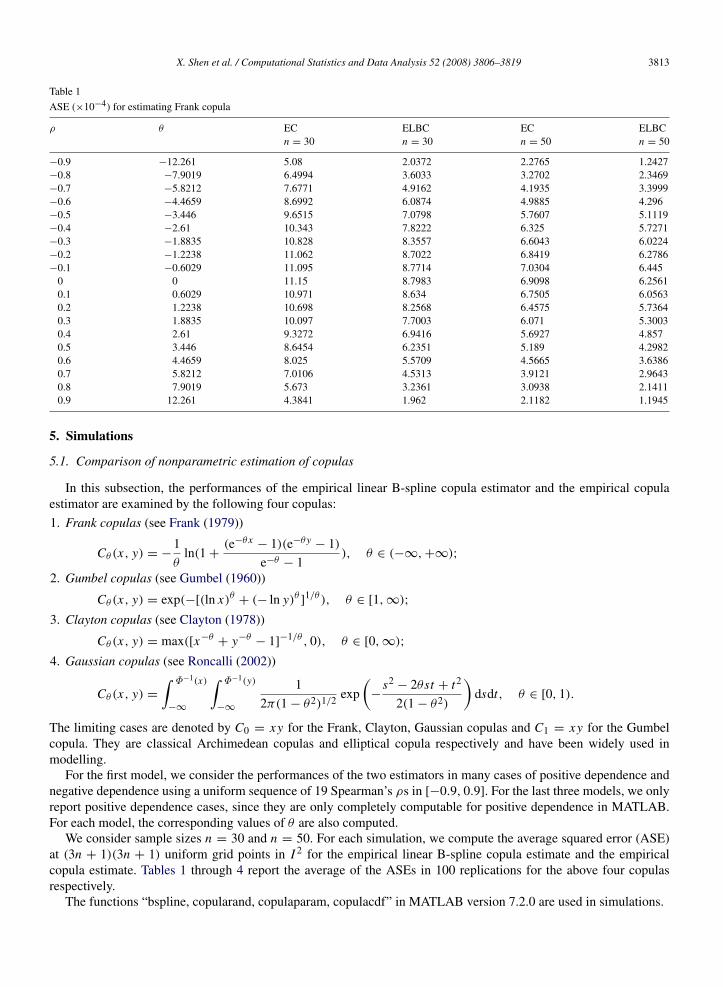
Table 1

ASE (×10−4) for estimating Frank copula

ρ θ EC ELBC EC ELBCn = 30 n = 30 n = 50 n = 50

−0.9 −12.261 5.08 2.0372 2.2765 1.2427−0.8 −7.9019 6.4994 3.6033 3.2702 2.3469−0.7 −5.8212 7.6771 4.9162 4.1935 3.3999−0.6 −4.4659 8.6992 6.0874 4.9885 4.296−0.5 −3.446 9.6515 7.0798 5.7607 5.1119−0.4 −2.61 10.343 7.8222 6.325 5.7271−0.3 −1.8835 10.828 8.3557 6.6043 6.0224−0.2 −1.2238 11.062 8.7022 6.8419 6.2786−0.1 −0.6029 11.095 8.7714 7.0304 6.445

0 0 11.15 8.7983 6.9098 6.25610.1 0.6029 10.971 8.634 6.7505 6.05630.2 1.2238 10.698 8.2568 6.4575 5.73640.3 1.8835 10.097 7.7003 6.071 5.30030.4 2.61 9.3272 6.9416 5.6927 4.8570.5 3.446 8.6454 6.2351 5.189 4.29820.6 4.4659 8.025 5.5709 4.5665 3.63860.7 5.8212 7.0106 4.5313 3.9121 2.96430.8 7.9019 5.673 3.2361 3.0938 2.14110.9 12.261 4.3841 1.962 2.1182 1.1945

5. Simulations

5.1. Comparison of nonparametric estimation of copulas

In this subsection, the performances of the empirical linear B-spline copula estimator and the empirical copulaestimator are examined by the following four copulas:

1. Frank copulas (see Frank (1979))

Cθ (x, y) = −1θ

ln(1 +(e−θx

− 1)(e−θy− 1)

e−θ − 1), θ ∈ (−∞, +∞);

2. Gumbel copulas (see Gumbel (1960))

Cθ (x, y) = exp(−[(ln x)θ + (− ln y)θ ]1/θ ), θ ∈ [1, ∞);

3. Clayton copulas (see Clayton (1978))

Cθ (x, y) = max([x−θ+ y−θ

− 1]−1/θ , 0), θ ∈ [0, ∞);

4. Gaussian copulas (see Roncalli (2002))

Cθ (x, y) =

∫ Φ−1(x)

−∞

∫ Φ−1(y)

−∞

1

2π(1 − θ2)1/2 exp(

−s2

− 2θst + t2

2(1 − θ2)

)dsdt, θ ∈ [0, 1).

The limiting cases are denoted by C0 = xy for the Frank, Clayton, Gaussian copulas and C1 = xy for the Gumbelcopula. They are classical Archimedean copulas and elliptical copula respectively and have been widely used inmodelling.

For the first model, we consider the performances of the two estimators in many cases of positive dependence andnegative dependence using a uniform sequence of 19 Spearman’s ρs in [−0.9, 0.9]. For the last three models, we onlyreport positive dependence cases, since they are only completely computable for positive dependence in MATLAB.For each model, the corresponding values of θ are also computed.

We consider sample sizes n = 30 and n = 50. For each simulation, we compute the average squared error (ASE)at (3n + 1)(3n + 1) uniform grid points in I 2 for the empirical linear B-spline copula estimate and the empiricalcopula estimate. Tables 1 through 4 report the average of the ASEs in 100 replications for the above four copulasrespectively.

The functions “bspline, copularand, copulaparam, copulacdf” in MATLAB version 7.2.0 are used in simulations.


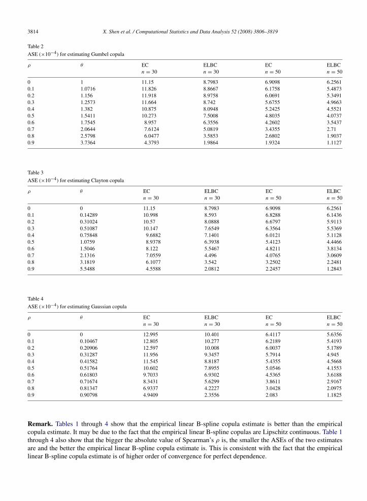
Table 2

ASE (×10−4) for estimating Gumbel copula


0 1 11.15 8.7983 6.9098 6.25610.1 1.0716 11.826 8.8667 6.1758 5.48730.2 1.156 11.918 8.9758 6.0691 5.34910.3 1.2573 11.664 8.742 5.6755 4.96630.4 1.382 10.875 8.0948 5.2425 4.55210.5 1.5411 10.273 7.5008 4.8035 4.07370.6 1.7545 8.957 6.3556 4.2602 3.54370.7 2.0644 7.6124 5.0819 3.4355 2.710.8 2.5798 6.0477 3.5853 2.6802 1.90370.9 3.7364 4.3793 1.9864 1.9324 1.1127

Table 3

ASE (×10−4) for estimating Clayton copula


0 0 11.15 8.7983 6.9098 6.25610.1 0.14289 10.998 8.593 6.8288 6.14360.2 0.31024 10.57 8.0888 6.6797 5.91130.3 0.51087 10.147 7.6549 6.3564 5.53690.4 0.75848 9.6882 7.1401 6.0121 5.11280.5 1.0759 8.9378 6.3938 5.4123 4.44660.6 1.5046 8.122 5.5467 4.8211 3.81340.7 2.1316 7.0559 4.496 4.0765 3.06090.8 3.1819 6.1077 3.542 3.2502 2.24810.9 5.5488 4.5588 2.0812 2.2457 1.2843

Table 4

ASE (×10−4) for estimating Gaussian copula


0 0 12.995 10.401 6.4117 5.63560.1 0.10467 12.805 10.277 6.2189 5.41930.2 0.20906 12.597 10.008 6.0037 5.17890.3 0.31287 11.956 9.3457 5.7914 4.9450.4 0.41582 11.545 8.8187 5.4355 4.56680.5 0.51764 10.602 7.8955 5.0546 4.15530.6 0.61803 9.7033 6.9302 4.5365 3.61880.7 0.71674 8.3431 5.6299 3.8611 2.91670.8 0.81347 6.9337 4.2227 3.0428 2.09750.9 0.90798 4.9409 2.3556 2.083 1.1825

Remark. Tables 1 through 4 show that the empirical linear B-spline copula estimate is better than the empiricalcopula estimate. It may be due to the fact that the empirical linear B-spline copulas are Lipschitz continuous. Table 1through 4 also show that the bigger the absolute value of Spearman’s ρ is, the smaller the ASEs of the two estimatesare and the better the empirical linear B-spline copula estimate is. This is consistent with the fact that the empiricallinear B-spline copula estimate is of higher order of convergence for perfect dependence.


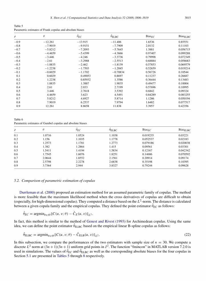
Table 5Parametric estimates of Frank copulas and absolute biases

ρ θ θEC θELBC BiasEC BiasELBC

−0.9 −12.261 −13.915 −11.406 1.6536 0.85551−0.8 −7.9019 −9.9151 −7.7909 2.0132 0.11103−0.7 −5.8212 −7.2093 −5.7645 1.3881 0.056715−0.6 −4.4659 −5.4399 −4.3666 0.97407 0.099288−0.5 −3.446 −4.246 −3.3736 0.79998 0.072349−0.4 −2.61 −3.2988 −2.5513 0.68884 0.058683−0.3 −1.8835 −2.462 −1.8139 0.57853 0.069579−0.2 −1.2238 −1.7503 −1.2045 0.52659 0.019214−0.1 −0.6029 −1.1702 −0.70834 0.56726 0.10544

0.1 0.6029 0.49053 0.8697 0.11237 0.266870.2 1.2238 0.85932 1.3586 0.36444 0.134830.3 1.8835 1.3887 1.9835 0.49477 0.100040.4 2.61 2.033 2.7199 0.57696 0.109950.5 3.446 2.7618 3.5392 0.6842 0.093240.6 4.4659 3.623 4.5491 0.84289 0.0832550.7 5.8212 4.6927 5.8714 1.1286 0.0501940.8 7.9019 6.2537 7.9794 1.6482 0.0775170.9 12.261 8.8658 11.838 3.3957 0.42356

Table 6Parametric estimates of Gumbel copulas and absolute biases


0.1 1.0716 1.0524 1.1038 0.019235 0.032210.2 1.156 1.1035 1.1778 0.052537 0.021830.3 1.2573 1.1781 1.2773 0.079186 0.0200380.4 1.382 1.2864 1.415 0.09561 0.033010.5 1.5411 1.4194 1.5834 0.12167 0.0423420.6 1.7545 1.6076 1.8251 0.14686 0.0705920.7 2.0644 1.8552 2.1561 0.20914 0.091740.8 2.5798 2.2278 2.6838 0.35198 0.103950.9 3.7364 2.944 3.8327 0.79244 0.09628

5.2. Comparison of parametric estimation of copulas

Durrleman et al. (2000) proposed an estimation method for an assumed parametric family of copulas. The methodis more feasible than the maximum likelihood method when the cross derivatives of copulas are difficult to obtain(especially, for high-dimensional copulas). They computed a distance based on the L2-norm. The distance is calculatedbetween a given copula family and the empirical copulas. They defined the point estimator θEC as follows:

θEC = argminθ∈Θ‖C(u, v; θ) − CE (u, v)‖L2 .

In fact, this method is similar to the method of Genest and Rivest (1993) for Archimedean copulas. Using the sameidea, we can define the point estimator θELBC based on the empirical linear B-spline copulas as follows:

θELBC = argminθ∈Θ‖C(u, v; θ) − CELB(u, v)‖L2 . (22)

In this subsection, we compare the performances of the two estimators with sample size of n = 30. We compute adiscrete L2 norm at (3n + 1)(3n + 1) uniform grid points in I 2. The function “fmincon” in MATLAB version 7.2.0 isused in simulations. The values of θEC and θELBC as well as the corresponding absolute biases for the four copulas inSection 5.1 are presented in Tables 5 through 8 respectively.


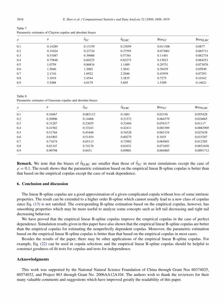
Table 7Parametric estimates of Clayton copulas and absolute biases


0.1 0.14289 0.13159 0.23059 0.011308 0.08770.2 0.31024 0.23724 0.37595 0.073001 0.0657110.3 0.51087 0.39686 0.57361 0.11401 0.0627340.4 0.75848 0.60225 0.82273 0.15623 0.0642510.5 1.0759 0.86834 1.1489 0.20751 0.0730760.6 1.5046 1.2002 1.5641 0.30439 0.059490.7 2.1316 1.6922 2.2046 0.43939 0.072930.8 3.1819 2.4544 3.2835 0.7275 0.101620.9 5.5488 4.0179 5.695 1.5309 0.14621

Table 8Parametric estimates of Gaussian copulas and absolute biases


0.1 0.10467 0.083112 0.1601 0.02156 0.0554280.2 0.20906 0.14468 0.23372 0.064379 0.0246650.3 0.31287 0.23655 0.32404 0.076317 0.011170.4 0.41582 0.33243 0.42411 0.083389 0.00829050.5 0.51764 0.45448 0.54528 0.063154 0.0276380.6 0.61803 0.51454 0.60275 0.1035 0.0152870.7 0.71674 0.65113 0.72902 0.065601 0.0122850.8 0.81347 0.74178 0.81031 0.071693 0.00316560.9 0.90798 0.8431 0.89881 0.064885 0.0091712

Remark. We note that the biases of θELBC are smaller than those of θEC in most simulations except the case ofρ = 0.1. The result shows that the parametric estimation based on the empirical linear B-spline copulas is better thanthat based on the empirical copulas except the case of weak dependence.

6. Conclusion and discussion

The linear B-spline copulas are a good approximation of a given complicated copula without loss of some intrinsicproperties. The result can be extended to a higher order B-spline which cannot usually lead to a new class of copulassince Eq. (13) is not satisfied. The corresponding B-spline estimation based on the empirical copulas, however, hassmoothing properties which may be more useful to analyze some concepts such as left tail decreasing and right taildecreasing behavior.

We have proved that the empirical linear B-spline copulas improve the empirical copulas in the case of perfectdependence. Simulation results given in this paper have also shown that the empirical linear B-spline copulas are betterthan the empirical copulas for estimating the nonperfectly dependent copulas. Moreover, the parametric estimationbased on the empirical linear B-spline copulas is better than that based on the empirical copulas in most cases.

Besides the results of the paper, there may be other applications of the empirical linear B-spline copulas. Forexample, Eq. (22) can be used in copula selection; and the empirical linear B-spline copulas should be helpful toconstruct goodness-of-fit tests for copulas and tests for independence.

Acknowledgments

This work was supported by the National Natural Science Foundation of China through Grant Nos 60374025,60574032, and Project 863 through Grant No. 2006AA12A104. The authors wish to thank the reviewers for theirmany valuable comments and suggestions which have improved greatly the readability of this paper.


Appendix

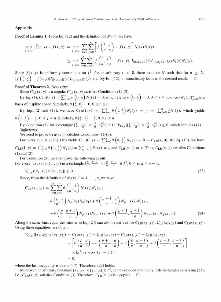
Proof of Lemma 1. From Eq. (12) and the definition of Ni (x), we have

supx,y∈I

| f (x, y) − f (x, y)| = supx,y∈I

∣∣∣∣∣ n∑i=0

n∑j=0

[f

(i

n,

j

n

)− f (x, y)

]Ni (x)N j (y)

∣∣∣∣∣≤ sup

x,y∈I

n∑i=0

n∑j=0

∣∣∣∣ f

(i

n,

j

n

)− f (x, y)

∣∣∣∣ I{[ti ,ti+2]}(x)I{[t j ,t j +2]}(y)Ni (x)N j (y).

Since f (x, y) is uniformly continuous on I 2, for an arbitrary ε > 0, there exits an N such that for n ≥ N ,

| f(

in ,

jn

)− f (x, y)|I{[ti ,ti+2]}(x)I{[t j ,t j +2]}(y) < ε. By Eq. (12), it immediately leads to the desired result. �

Proof of Theorem 2. Necessity:Since CLB(x, y) is a copula, CLB(x, y) satisfies Conditions (1)–(3).

By Eq. (1), CLB(0, y) =∑n

j=0 θ(

0,jn

)N j (y) = 0, which yields θ

(0,

jn

)= 0, 0 ≤ j ≤ n, since {N j (y)}n

j=0 is a

basis of a spline space. Similarly, θ( i

n , 0)

= 0, 0 ≤ i ≤ n.

By Eqs. (2) and (13), we have CLB(1, y) =∑n

j=0 θ(

1,jn

)N j (y) = y =

∑nj=0

jn Ni (y), which yields

θ(

1,jn

)=

jn , 0 ≤ j ≤ n. Similarly, θ

( in , 1

)=

in , 0 ≤ i ≤ n.

By Condition (3), for a rectangle [in , i+1

n ] × [jn ,

j+1n ] in I 2, VCLB([ i

n , i+1n ] × [

jn ,

j+1n ]) ≥ 0, which implies (17).

Sufficiency:We need to prove CLB(x, y) satisfies Conditions (1)–(3).

For every x, y ∈ I , Eq. (16) yields CLB(0, y) =∑n

j=0 θ(

0,jn

)N j (y) = 0 = CLB(x, 0). By Eq. (13), we have

CLB(1, y) =∑n

j=0 θ(

1,jn

)N j (y) =

∑nj=0

jn N j (y) = y and CLB(x, 1) = x . Thus, CLB(x, y) satisfies Conditions

(1) and (2).For Condition (3), we first prove the following result.

For every [x1, x2] × [y1, y2] in a rectangle [pn ,

p+1n ] × [

qn ,

q+1n ] ∈ I 2, 0 ≤ p, q ≤ n − 1,

VCLB([x1, x2] × [y1, y2]) ≥ 0. (23)

Since, from the definition of Ni (x), i = 1, . . . , n, we have

CLB(x1, y1) =

n∑i=0

n∑j=0

θ

(i

n,

j

n

)Ni (x1)N j (y1)

= θ( p

n,

q

n

)Np(x1)Nq(y1) + θ

(p + 1

n,

q

n

)Np+1(x1)Nq(y1)

+ θ

(p

n,

q + 1n

)Np(x1)Nq+1(y1) + θ

(p + 1

n,

q + 1n

)Np+1(x1)Nq+1(y1). (24)

Along the same line, equalities similar to Eq. (24) can also be derived for CLB(x1, y2), CLB(x2, y1) and CLB(x2, y2).Using these equalities, we obtain

VCLB ([x1, x2] × [y1, y2]) = CLB(x1, y1) − CLB(x1, y2) − CLB(x2, y1) + CLB(x2, y2)

=

[θ

( p

n,

q

n

)− θ

(p + 1

n,

q

n

)− θ

(p

n,

q + 1n

)+ θ

(p + 1

n,

q + 1n

)]× [n2(x1 − x2)(y1 − y2)]

≥ 0,

where the last inequality is due to (17). Therefore, (23) holds.Moreover, an arbitrary rectangle [x1, x2] × [y1, y2] ∈ I 2, can be divided into many little rectangles satisfying (23),

i.e., CLB(x, y) satisfies Condition (3). Therefore, CLB(x, y) is a copula. �


Proof of Theorems 3–6. By the definition of the linear B-spline copulas and the properties of the linear B-splines,one can prove the results directly. We omit the details of the proofs as they are straightforward but tedious. �

Proof of Theorem 7. Since

supx,y∈I

|CELB(x, y) − C(x, y)| ≤ supx,y∈I

|CELB(x, y) − C(x, y)| + supx,y∈I

|C(x, y) − C(x, y)|, (25)

where C(x, y) =∑n

i=0∑n

j=0 C(

in ,

jn

)Ni (x)N j (y), applying Lemma 1 yields

supx,y∈I

|C(x, y) − C(x, y)| → 0. (26)

In addition, by Eq. (12),

supx,y∈I

∣∣∣CELB(x, y) − C(x, y)

∣∣∣ = supx,y∈I

∣∣∣∣∣ n∑i=0

n∑j=0

[CE

(i

n,

j

n

)− C

(i

n,

j

n

)]Ni (x)N j (y)

∣∣∣∣∣≤ sup

x,y∈I

∣∣∣∣∣ n∑i=0

n∑j=0

[ sups,t∈I

|CE (s, t) − C(s, t)|]Ni (x)N j (y)

∣∣∣∣∣≤ sup

s,t∈I|CE (s, t) − C(s, t)|.

By the Glivenko–Cantelli lemma, sups,t∈I |CE (s, t) − C(s, t)| → 0, a.s. Then, we have

supx,y∈I

|CELB(x, y) − C(x, y)| → 0, a.s. (27)

Therefore, by (25)–(27), we have supx,y∈I | CELB(x, y) − C(x, y) |→ 0, a.s., as n → ∞. �

Proof of Theorem 8. Since√

n(CELB(x, y) − C(x, y)) =√

n(CE (x, y) − C(x, y)) +√

n(CELB(x, y) − CE (x, y)),one can apply Theorem 4 of Fermanian et al. (2004) to obtain

√n(CE (x, y) − C(x, y)) converges weakly to the

Gaussian process GC in l∞([0, 1]2) which is given in (21). In addition,

√n sup

x,y∈I|CELB(x, y) − CE (x, y)|

=√

n supx,y∈I

∣∣∣∣∣ n∑i=0

n∑j=0

(CE

(i

n,

j

n

)− CE (x, y)

)Ni (x)N j (y)

∣∣∣∣∣=

√n sup

x,y∈I

∣∣∣∣∣ n∑i=0

n∑j=0

[CE

(i

n,

j

n

)− CE (x, y)

]I{[ti ,ti +2]}(x)I{[t j ,t j +2]}(y)Ni (x)N j (y)

∣∣∣∣∣≤

√n sup

x,y∈I

∣∣∣∣∣ n∑i=0

n∑j=0

4n

Ni (x)N j (y)

∣∣∣∣∣ a.s.

= op(1).

Then, one can obtain the result from the Slutsky theorem. �

References

Cherubini, U., Luciano, E., Vecchiato, W., 2004. Copula Methods in Finance. Wiley, UK.Clayton, D.G., 1978. A model for association in bivariate life tables and its application in epidemiological studies of familial tendency in chronic

disease incidence. Biometrika 65, 141–151.Curry, H.B., Schoenberg, I.J., 1966. On Polya frequency functions IV: The fundamental spline functions and their limits. J. Analyse Math. 17,

71–107.de Boor, C., 1978. A Practical Guide to Splines. Springer-Verlag, New York.Deheuvels, P., 1979. La fonction de dependance empirique et ses proprietes. Acad. Roy. Belg., Bull. Cl Sci. 5ieme ser. 65, 274–292.


Deheuvels, P., 1981a. A Kolmogorov–Smirnov Type Test for independence and multivariate samples. Rev. Roumaine Math. Pures Appl. 26 (2),213–226.

Deheuvels, P., 1981b. A nonparametric test for independence. Publ. Inst. Statist. Univ. Paris. 26 (2), 29–50.Denuit, M., Scaillet, O., 2004. Nonparametric tests for positive quadrant dependence. J. Finan. Econ. 2, 422–450.Dhaene, J., Goovaerts, M., 1996. Dependency of risks and stop-loss order. ASTIN Bulletin. 26, 201–212.Durrleman, V., Nikeghbali, A., Roncalli, T., 2000. Which copula is the right one? working document, Groupe de Recherche Operationnelle, Credit

Lyonnais.Embrechts, P., McNeil, A., Straumann, D., 2002. Correlation and dependence properties in risk management: Properties and Pitfalls.

In: Dempster, M. (Ed.), Risk Management: Value at Risk and Beyond. Cambridge University press, pp. 176–223.Fermanian, J.D., Radulovic, D., Wegkamp, M., 2004. Weak convergence of empirical copula processes. Bernoulli 10 (5), 847–860.Fermanian, J.D., Scaillet, O., 2003. Nonparametric estimation of copulas for time series. J. Risk. 5, 25–54.Frank, M.J., 1979. On the simultaneous associativity of F(x, y) and x + y − F(x, y). Aequationes Math. 19, 194–226.Gaenssler, P., Stute, W., 1987. Seminar on Empirical Processes, DMV Sem. 9. Birkhauser, Basel.Genest, C., Rivest, L.P., 1993. Statistical inference procedures for bivariate Archimedean copulas. J. Amer. Statist. Assoc. 88, 1034–1043.Genest, C., Ghoudi, K., Rivest, L.P., 1995. A semiparametric estimation procedure of dependence parameters in multivariate families of

distributions. Biometrika. 82, 534–552.Gumbel, E.J., 1960. Bivariate exponential distributions. J. Amer. Statist. Assoc. 55, 698–707.Joe, H., 1997. Multivariate Models and Dependence Concepts. Chapman and Hall, London.Joe, H., Xu, J.J., 1996. The estimation method of inference functions for margins for multivariate models. Dept. of Statistics University of British

Columbia. Tech. Rept. 166.Kim, G., Silvapulle, M.J., Silvapulle, P., 2007. Comparison of semiparametric and parametric methods for estimating copulas. Comput. Statist.

Data. Anal 6 (51), 2836–2850.Lehmann, E., 1966. Some concepts of dependence. Ann. Math. Statist. 37, 1137–1153.Nelsen, R.B., 1993. Some concepts of bivariate symmetry. J. Nonparametr. Stat. 3, 95–101.Nelsen, R.B., 1999. An Introduction to Copulas. Springer-Verlag, New York.Nurnberger, G., 1989. Approximation by Spline Functions. Springer-Verlag, New York.Roncalli, T., 2002. Gestiondes Risques Multiples. Cours ENSAI de 3e annee. Groupe de Recherche Operationelle, Credit Lyonnais, Working paper.Scaillet, O., 2005. A Kolmogorov–Smirnov type test for positive quadrant dependence. Canad. J. Statist. 33 (2).Schweizer, B., Wolff, E.F., 1981. On nonparametric measures of dependence for random variables. Ann. Statist. 9, 879–885.Sklar, A., 1959. Fonctions de repartition an dimensions et leurs marges. Publ. Inst. Statist.Univ. Paris. 8, 229–231 (in French).Vaart, A.W.van der., Wellner, J.A., 1996. Weak Convergence and Empirical Processes. Springer-Verlag, New York.

linear b-spline copulas with applications to nonparametric estimation of copulas

Documents