linear algebra and its applications978 p.n. shivakumar, k.c. sivakumar / linear algebra and its...
TRANSCRIPT

Linear Algebra and its Applications 430 (2009) 976–998
Contents lists available at ScienceDirect
Linear Algebra and its Applications
j ourna l homepage: www.e lsev ie r .com/ loca te / laa
A review of infinite matrices and their applications
P.N. Shivakumar a,∗, K.C. Sivakumar b
a Department of Mathematics, University of Manitoba, Winnipeg, Manitoba, Canada R3T 2N2b Department of Mathematics, Indian Institute of Technology Madras, Chennai 600 036, India
A R T I C L E I N F O A B S T R A C T
Article history:
Received 1 September 2006
Accepted 21 September 2008
Available online 22 November 2008
Submitted by D. Hershkowitz
Keywords:
Finite matrices
Infinite matrices
Eigenvalues
Generalized inverses
Infinite matrices, the forerunner and a main constituent of many
branchesof classicalmathematics (infinitequadratic forms, integral
equations, differential equations, etc.) and of the modern opera-
tor theory, is revisited to demonstrate its deep influence on the
development ofmany branches ofmathematics, classical andmod-
ern, replete with applications. This review does not claim to be
exhaustive, but attempts to present research by the authors in a
variety of applications. These include the theory of infinite and
related finite matrices, such as sections or truncations and their
relationship to the linear operator theory on separable and se-
quence spaces. Matrices considered here have special structures
like diagonal dominance, tridiagonal, sign distributions, etc. and
are frequently nonsingular. Moreover, diagonally dominant finite
and infinite matrices occur largely in numerical solutions of ellip-
tic partial differential equations. The main focus is the theoretical
and computational aspects concerning infinite linear algebraic and
differential systems, using techniques like conformal mapping,
iterations, truncations, etc. to derive estimates based solutions.
Particular attention is paid to computable precise error estimates,
and explicit lower and upper bounds. Topics include Bessel’s, Mat-
hieu equations, viscous fluid flow, simply and doubly connected
regions, digital dynamics, eigenvaluesof theLaplacian, etc.Alsopre-
sented are results in generalized inverses and semi-infinite linear
programming.
© 2008 Elsevier Inc. All rights reserved.
∗ Corresponding author.
E-mail addresses: [email protected] (P.N. Shivakumar), [email protected] (K.C. Sivakumar).
0024-3795/$ - see front matter © 2008 Elsevier Inc. All rights reserved.
doi:10.1016/j.laa.2008.09.032

P.N. Shivakumar, K.C. Sivakumar / Linear Algebra and its Applications 430 (2009) 976–998 977
1. Introduction
In mathematical formulation of physical problems and their solutions, infinite matrices arise more
naturally than finite matrices. In the past, infinite matrices played an important role in the theory
of summability of sequences and series. The book “Infinite Matrices,” by Cooke [9] is perhaps the
first one to deal with infinite matrices. It also gives a clear indication of the role of infinite matrices
as applied to topics like quantum mechanics, spectral theory and linear operators in the context of
functional abstract Hilbert spaces. An excellent detailed account of the colorful history of infinite
matrices is given by Bernkopf [6]. Infinite matrices and determinants were introduced into analysis
by Poincare in 1884 in the discussion of the well known Hill’s equation. In 1906, Hilbert used infinite
quadratic forms (which are equivalent to infinite matrices) to discuss the solutions of Fredholm inte-
gral equations. Within a few years, many theorems fundamental to the theory of abstract operators
on function spaces were discovered although they were expressed in special matrix terms. In 1929,
John von Neumann showed that an abstract approach was powerful and preferable to using infinite
matrices as a tool for the study of operators. The tools of functional analysis establish in a limited
number of cases, qualitative results such as existence, uniqueness and in some cases justification of
truncation, but the results are of generally little use in deriving explicit, computable and meaningful
error bounds needed for approximate or computational work. A main source for infinite matrices
has been including solutions of ordinary and partial differential equations. In this review, we con-
centrate on particular structures for matrices, finite and infinite. Infinite matrices occur in numerous
applications. A brief list, in addition to those presented in this review, includes inversion of Laplace
Transforms, biorthogonal infinite sets, generalized moments, interpolation, Sobolev spaces, signal
processing, time series, ill-posed problems and birth–death problems. In particular, we deal with
diagonally dominant matrices (full and tridiagonal), sign distributions, etc. The advantage of such
matrices lies in knowing estimates for the inverse elements replete with an error analysis which
also includes lower and upper bounds. This review reflects the interests of the authors and is in-
tended to demonstrate, although in a limited context, the influence of the discussion on a variety of
problems in applied mathematics and physics. In what follows, our main aim is to get meaningful,
computable error bounds in which process, existence and uniqueness of solutions of infinite sys-
tems fall out as a bonus. Sections 2–8 consist of theoretical considerations, while Section 9 gives
a variety of applications. As our analysis of various problems start with finite matrices obtained
by truncating infinite matrices, Section 2, discusses nonsingularity conditions and provides some
easily computable estimates for upper and lower bounds concerning the inverse and its elements.
Infinite linear algebraic systems Ax = b are considered in Section 3, where analytical results and error
estimates for the the truncated system and the infinite system are given. Section 4 discusses the linear
eigenvalue problem Ax = λx for the infinite case, where the eigenvalues are boxed in non overlapping
intervals using estimates for the inverse. This enables us to calculate any eigenvalue to any required
degree of accuracy. Linear differential systems of the form dx/dt = Ax + f constitute discussions in
Section 5. Here also, truncations are used to establish existence, uniqueness and approximations
with error analysis, under stated conditions on A, and f . Section 6 considers iterative methods for
Tx = v, where x, v belong to �∞ and T is a linear bounded operator on �∞. To our knowledge, iteration
techniques used here for infinite systems open up avenues for further research. A novel computational
technique involving determinants and their estimates to locate eigenvalues is described in Section
7. This intricate technique is used later on when discussing solutions of Mathieu equations. Some
interesting results on nonuniqueness of the Moore–Penrose inverse are given in Section 8. A number
of applications are given in Section 9. These include classical conformal mapping problems, fluid
and gas flow in pipes, eigenvalues of Mathieu equations, iteration techniques for Bessel’s equation,
vibrating membrane with a hole, differential equations on semi-infinite intervals, semi-infinite lin-
ear programming, groundwater flow problem and determination of eigenvalues of the Laplacian
in an elliptic region. Other linear problems include analysis of solutions on semi-infinite intervals
of the differential equation y′′ + f (x)y = 0, with f (x) → ∞ [30] and using finite difference methods
[8].

978 P.N. Shivakumar, K.C. Sivakumar / Linear Algebra and its Applications 430 (2009) 976–998
2. Finite matrices and their inverses
In this section we give three different criteria for an n × n matrix A = (aij) to be nonsingular. We
also give in these cases some estimates for the inverse elements of A−1(= Aji
detA
)where Aji represents
the cofactor of aij and detA is the determinant of A.
(a) Diagonal dominance
Writing
σi|aii| =n∑
j=1,j /=i
|aij|, 0 � σi < 1, i = 1, 2, . . . ,n. (2.1)
A is called diagonally row dominant (d.d.), if σi � 1 and strictly diagonally row dominant (s.d.d), if
σi < 1, i = 1, . . . ,n. Similar definitions hold good for columns. There are a number of proofs showing
that A is nonsingular if A is s.d.d. A is a tri-diagonal matrix denoted by {ai, bi, ci}, where bi, i = 1, . . . ,n
denote diagonal elements and ai, i = 2 . . . ,n denote the lower diagonal elements and ci, i = 1, . . . ,n − 1
denote the upper diagonal elements.
For the finite linear system
n∑j=1
aijxj = bi, i = 1, 2, . . . ,n (2.2)
or
Ax = b,
we have by Cramer’s rule,
x = A−1b, xj =n∑
k=1
Akj
detAbk , j = 1, 2, . . . ,n. (2.3)
There have been many generalizations of the concept of diagonal dominance and an equivalent
theorem is given by Varga [43]:
Let N = {1, 2, . . . ,n} and
J =⎧⎨⎩i ∈ N : |aii| >
∑j /=i
|aij|⎫⎬⎭ /= ∅. (2.4)
If J = N, then A is strictly row d.d. and hence detA does not vanish [3]. If A is irreducible, then A is
nonsingular [41].
Using (2.1) with σi < 1, i = 1, 2, . . .n, we have the following results [15]:
detA /= 0,
|Aij| � σj|Aii|, i /= j∣∣∣∣ Aii
detA
∣∣∣∣ � 1
|aii|(1 − σi), i = 1, 2, . . . ,n. (2.5)
Setting α = mink{|akk(1 − σk)|}, Varah [42] establishes that
‖A−1‖∞ = maxi
n∑k=1
|Aki|detA
<1
α. (2.6)
Further, if aii > 0, aij � 0, i /= j, then A is nonsingular and A−1 � 0 so that A is anM-matrix.
(b) A chain condition
If for thematrixA = (aij), an n × ndiagonally dominantmatrix,which satisfies (2.4), there exists, for
each i /∈ J, a sequence of nonzero elements of the form ai,i1 , ai,i2 , . . . , ai,ij with j ∈ J, then A is nonsingular

P.N. Shivakumar, K.C. Sivakumar / Linear Algebra and its Applications 430 (2009) 976–998 979
[24]. The proof of this result depends on an earlier result by Ky Fan, who has shown that for a matrix
A(= aij) and anM-matrix B(= bij) where |bii| � |aii| for all i ∈ N and |aij| � |bij| for i /= j, the inequality
detA � det B holds. This result extends to cases where A is reducible and satisfies the chain condition.
We will use this chain condition later in the application to digital circuit dynamics.
(c) Tridiagonal matrices
We consider here diagonally dominant tridiagonal matrices A = {ai, bi, ci} with
μi|bi| = |ai| + |ci|, 0 � μi � 1, i = 1, 2, . . . ,n, ai, bi, ci /= 0. (2.7)
Ostrowski [15] gave the following upper bounds for the inverse elements of a full s.d.d. n × n matrix
B(= bij)∣∣∣∣ Bjj
det B
∣∣∣∣ � 1
|bjj|(1 − μj)
and
|Bij| � λj|Bii|,where
λi|bii| =∑j /=i
|bij|, 0 � λi � 1, i = 1, 2, . . . ,n. (2.8)
In [32], Shivakumar and Ji improvee Ostrowski’s bounds and further gave lower bounds for finite
tridiagonal s.d.d. matrices. The improved bounds for i � j are given by⎛⎝ j∏k=i+1
|ak||bk|(1 + μk)
⎞⎠ |Aii| � |Aij| �⎛⎝ j∏
k=i+1
μk
⎞⎠ |Aii|, (2.9)
∣∣∣∣ajai∣∣∣∣⎛⎝j−1∏
k=i
|ak||bk|(1 + μk)
⎞⎠ |Ajj| � |Aij| �∣∣∣∣ajai
∣∣∣∣⎛⎝j−1∏
k=i
μk
⎞⎠ |Ajj| (2.10)
with similar results for i � j.
Further
1
|bi| + |ai|μi−1 + |ci|μi+1�∣∣∣∣ Aii
detA
∣∣∣∣ � 1
|bi| − |ai|μi−1 − |ci|μi+1, (2.11)
where μ0 = μn+1 = 0.
For inverse elements of A, we have for i � j,∏jk=i+1
|ak|∏jk=i
|bk|(1 + μk)�∣∣∣∣ Aij
detA
∣∣∣∣ �∏j
k=i+1μk
|bi| − |ai|μi−1 − |ci|μi+1(2.12)
with similar results for i � j.
In many applications, we need an upper bound for ‖A−1‖∞. This is given by
‖A−1‖∞ � 1
δ(1 − μ),
where
μ = supk
{μk}, δ = infk
{|bk|}.
Note that the inequality fails if some of the μ’s are 1.
This result has been extended where the tridiagonal matrix is an infinite matrix. As an example,
we quote the following theorem [32]:
For the matrix A defined above,
‖A−1‖∞ <2(rn+1 − r
n+12
)δr3
, (2.13)

980 P.N. Shivakumar, K.C. Sivakumar / Linear Algebra and its Applications 430 (2009) 976–998
where μk < 1,μi = 1, for i /= k, q = minl
{ |al ||bl | ,
|cl ||bl |}and r = (1+q)
q > 2, δ = infk{|bk|}.(d) Some sign patterns
A newnonsingularity criteria for an n × n realmatrix A, based on sign distributions and some stated
conditions on the elements of A is given. This work is motivated by the solution of Poisson’s equation
for doubly connected regions (see Section 9.2). Nonsingularity related to M-matrices and positive
matrices, with fixed sign distributions, have been extensively studied by Fiedler, Fan, Householder,
Drew and Johnson (for details of see [35]).
Wenowgive a set of earlier verifiable sufficient conditions for amatrixA to be nonsingular based on
sign distribution and some easily computable sufficient conditions on the elements of A. We consider
the sign distribution for the m × m matrix A, which ensures nonsigularity of A are given as follows
[35]:
We consider the sign distribution for them × mmatrix A, given as follows [35]: aij > 0 for i � j and
(−1)i+jaij > 0 for i > j, i, j = 1, 2, . . . ,m. (2.14)
For convenience we define for i � j,
νij = aij −m∑
k=j+1
aik (2.15)
and
μij = aij −i−1∑k=1
aij (2.16)
and for j � i < l < m,
ωlij = min
⎧⎨⎩|aij| −∣∣∣∣∣∣
l∑k=i+1
akj
∣∣∣∣∣∣ ,∣∣∣∣∣∣
l∑k=i+1
akj
∣∣∣∣∣∣− |al+1,j|⎫⎬⎭ (2.17)
and
δijl =∣∣∣∣∣∣
l∑k=j+1
aik
∣∣∣∣∣∣− ∣∣aij∣∣ for j < l � i. (2.18)
3. Linear algebraic systems
We are concerned here with the infinite system of linear equations [21]:
∞∑j=1
aijxj = bi, i = 1, 2, . . . ,∞, (3.1)
or alternatively
Ax = b, (3.2)
where the infinite matrix A = (aij), is s.d.d., i.e,
σi|aii| =∞∑j=1
|aij|; 0 � σi < 1; i = 12, . . . ,∞ (3.3)
and the sequence {bi} is bounded. We establish sufficient conditions which guarantee the
existence and uniqueness of a bounded solution to (3.1). The infinite case is approached by finite
truncations and use of results in Section 2. In classical analysis, linear equations in infinite matrices
occur in interpolation, sequence spaces, summability and the present case occurs in solution of ellip-
tic partial differential equations in multiply connected regions. Our approach is to initially develop
estimates for the truncated system
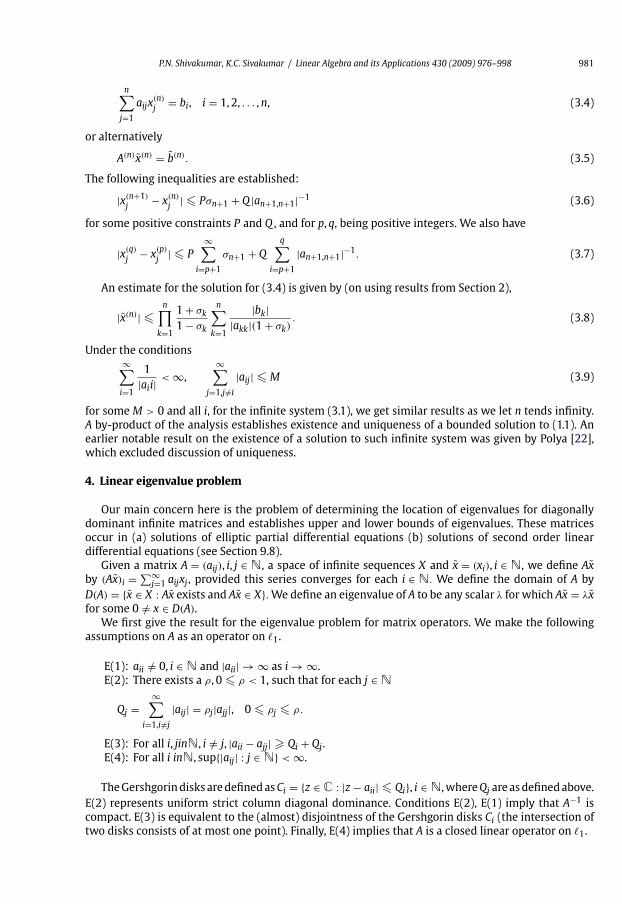
P.N. Shivakumar, K.C. Sivakumar / Linear Algebra and its Applications 430 (2009) 976–998 981
n∑j=1
aijx(n)
j= bi, i = 1, 2, . . . ,n, (3.4)
or alternatively
A(n)x(n) = b(n). (3.5)
The following inequalities are established:
|x(n+1)
j− x
(n)
j| � Pσn+1 + Q |an+1,n+1|−1 (3.6)
for some positive constraints P and Q , and for p, q, being positive integers. We also have
|x(q)j
− x(p)
j| � P
∞∑i=p+1
σn+1 + Q
q∑i=p+1
|an+1,n+1|−1. (3.7)
An estimate for the solution for (3.4) is given by (on using results from Section 2),
|x(n)| �n∏
k=1
1 + σk
1 − σk
n∑k=1
|bk||akk|(1 + σk)
. (3.8)
Under the conditions∞∑i=1
1
|aii|< ∞,
∞∑j=1,j /=i
|aij| � M (3.9)
for some M > 0 and all i, for the infinite system (3.1), we get similar results as we let n tends infinity.
A by-product of the analysis establishes existence and uniqueness of a bounded solution to (1.1). An
earlier notable result on the existence of a solution to such infinite system was given by Polya [22],
which excluded discussion of uniqueness.
4. Linear eigenvalue problem
Our main concern here is the problem of determining the location of eigenvalues for diagonally
dominant infinite matrices and establishes upper and lower bounds of eigenvalues. These matrices
occur in (a) solutions of elliptic partial differential equations (b) solutions of second order linear
differential equations (see Section 9.8).
Given a matrix A = (aij), i, j ∈ N, a space of infinite sequences X and x = (xi), i ∈ N, we define Ax
by (Ax)i = ∑∞j=1 aijxj , provided this series converges for each i ∈ N. We define the domain of A by
D(A) = {x ∈ X : Ax exists and Ax ∈ X}. We define an eigenvalue of A to be any scalar λ for which Ax = λx
for some 0 /= x ∈ D(A).
We first give the result for the eigenvalue problem for matrix operators. We make the following
assumptions on A as an operator on �1.
E(1): aii /= 0, i ∈ N and |aii| → ∞ as i → ∞.
E(2): There exists a ρ, 0 � ρ < 1, such that for each j ∈ N
Qj =∞∑
i=1,i /=j
|aij| = ρj|ajj|, 0 � ρj � ρ.
E(3): For all i, jinN, i /= j, |aii − ajj| � Qi + Qj .
E(4): For all i inN, sup{|aij| : j ∈ N} < ∞.
TheGershgorindisks aredefinedasCi = {z ∈ C : |z − aii| � Qi}, i ∈ N,whereQj areasdefinedabove.
E(2) represents uniform strict column diagonal dominance. Conditions E(2), E(1) imply that A−1 is
compact. E(3) is equivalent to the (almost) disjointness of the Gershgorin disks Ci (the intersection of
two disks consists of at most one point). Finally, E(4) implies that A is a closed linear operator on �1.

982 P.N. Shivakumar, K.C. Sivakumar / Linear Algebra and its Applications 430 (2009) 976–998
For an operator A on �1 with E(1) and E(2), it is shown in [28, Theorem 2] that A is an opera-
tor with dense domain, R(A) = �1, A is compact on �1 and ‖A−1‖ is compact on �1, and ‖A−1‖1 �(1 − e)−1(inf i |aii|)−1. The main result for an operator A on �1 with E(1)–E(4), is that the operator A
consists of a discrete countable set of non zero eigenvalues {λk : k ∈ N} such that |λk| → ∞ as k → ∞.
Similar results are also derived for operators on �∞. For an operator A on �∞ consider:
E(5): There exists a σ , 0 � σ < 1, such that for each i ∈ N,
Pi =∞∑
j=1,j /=i
|aij| = σi|aii|, 0 � σi � σ.
E(6): For all i, j ∈ N, i /= j, |aii − ajj| � Pi + Pj .
E(7): For all j, supj{|aij| : i ∈ N} < ∞.
Analogous to the above, let Ri = {z ∈ C : |z − aii| � Pi}, i ∈ N.
We also note that E(5) implies uniform strict row diagonal dominance and E(6) is equivalent to the
(almost) disjointness of the Gershgorin disks Ri.
For an operator A on �∞ with E(1), E(5), E(7), it is proved that [28] A is a closed operator, R(A) =�∞,A−1 is compact on �∞ and ‖A−1‖∞ � (1 − σ)−1(inf i |aii|)−1. Also, the spectrum of A consists of
discrete countable set of nonzero eigenvalues {λk : k ∈ N} such that |λk| → ∞ as k → ∞. These results
give a complete description of all the eigenvalues for a (matrix) operator on �1 and �∞.
Further, in [28], truncation of the system Ax = y and corresponding error analysis are studied in
detail.
5. Linear differential systems
We consider the infinite system
d
dtxi(t) =
∞∑j=1
aijxj(t) + fi(t), t � 0, xi(0) = yi, i = 1, 2, . . . , (5.1)
which can be written as
˙x(t) = Ax(t) + f (t), ˙x(0) = y (5.2)
is of considerable theoretical and applied interest. In particular, such systems occur frequently in the
theoryof stochasticprocesses,perturbation theoryofquantummechanics, degradationofpolynomials,
infinite ladder network theory, etc. Arley and Brochsenius 1944, Bellman 1947, Shaw 1973 are the
notable ones who have studied problem (5.2). In particular, if A is a bounded operator on �1, then the
convergence of a truncated system has been established. However, none of these papers yields explicit
error bounds for such a truncation, where [26] provides such error bounds.
We consider (5.2) rewritten as ˙x = Ax + f , x(0) = y, where x, y and f are infinite column vectors in X ,
and A is a constant infinite matrix defining a bounded operator on X , where X is �1, c0 (the space of real
convergent sequences converging to zero or �∞). Consider the following assumptions for homogeneous
systems (f = 0):
DS(1): M = ∑∞i=1 |yi| < ∞.
DS(2): α = sup{∑∞i=1 |aij|, j = 1, 2, . . . ,∞} < ∞.
DS(3): γn = sup{∑∞i=n+1 |aij|, j = 1, 2, . . . ,n} → 0 as n → ∞.
DS(4): δn = sup{∑ni=1 |aij|, j = 1, 2, . . . ,n} → 0 as n → ∞.
In the above, DS(1) states that y ∈ �1. DS(2) is equivalent to the statement that A is bounded on
�1. DS(3) states that the sums in DS(2) converge uniformly below the main diagonal; it is a condition
involving only the entries of A below themain diagonal. DS(4) is a condition involving only the entries
of A above the main diagonal; it is somewhat less natural than DS(3).

P.N. Shivakumar, K.C. Sivakumar / Linear Algebra and its Applications 430 (2009) 976–998 983
In [26, Theorem 1] for the homogeneous linear system of differential equations as given above,
suppose that DS(1), DS(2) and either DS(3) or DS(4) hold. It is then shown that limn→∞ x(n)(t) = x(t)
in l1-norm uniformly in t on compact subsets of [0,∞), with explicit error bounds as given below:
n∑i=1
|xi(t) − x(n)
i(t)| � αteαt
⎡⎣1
2γnMt +
∞∑k=n+1
|yk|⎤⎦ , (5.3)
∞∑i=n+1
|xi(t)| � eαt
⎡⎣γnMt +∞∑
k=n+1
|yk|⎤⎦ , (5.4)
‖x(t) − x(n)(t)‖ � eαt
⎡⎣(1 + 1
2αt
)γnMt + (1 + αt)
∞∑k=n+1
|yk|⎤⎦ (5.5)
for DS(3) (with the right hand side converging to zero as n → ∞) and
n∑i=1
|xi(t) − x(n)
i(t)| � δnMteαt (5.6)
for DS(4) (with the right hand side converging to zero as n → ∞.)
For the nonhomogeneous system, consider the assumption
DS(5): fi(t) is continuous on [0,∞), i = 1, 2, . . ., and ‖f (t)‖ = ∑∞i=1 |fi(t)| converges uniformly in t on
compact subsets of [0,∞).
Define L(t) = sup{‖f (τ )‖ : 0 � τ � t}.DS(5) is equivalent to the statement that f (t) is continuous from [0,∞) into �1 and this implies that
L(t) < ∞ for all t � 0.
For the nonhomogeneous case we have the following result [26, Theorem 2], if DS(2), DS(5) and
either DS(3) or DS(4) hold, then limn→∞ x(n)(t) = x(t) in l1 norm uniformly in t on compact subsets of
[0,∞), with explicit error bounds as given below:
‖x(t) − x(n)(t)‖ � 1
2t2eαtγnL(t) + teαt sup
⎧⎨⎩∞∑
k=n+1
|fk(τ )| : 0 � τ � t
⎫⎬⎭ (5.7)
for DS(3) (with the right hand side converging to zero as n → ∞) and
n∑i=1
|xi(t) − x(n)
i(t)| � δnL(t)α
−2[αteαt + (1 − eαt)] (5.8)
for DS(4) (with the right hand side converging to zero as n → ∞).
Similar results hold for systems on l1 [26, Theorems 4 and 6] and for systems on c0 [26, Theorems
3 and 5].
The analysis above concerns A, being a constant infinite matrix defining a bounded operator on E,
where E is �1, c0 or �∞. Explicit error bounds are obtained for the approximation of the solution of the
infinite system by the solutions of finite truncation systems.
6. An iterative method
Iterativemethods for linear equations in finitematrices have been the subject of very vast literature
which is still growing due to the advent of finite elements. Since allmethods involve the nonsingularity
of thematrix, d.d. matrices have played amajor role. Our interest here is to discuss an iterativemethod
for such infinite systems which we believe to be one of the first such attempts.
For the finite system I.d.d. matrices were introduced by Chew and Shivakumar [27] where s.d.d.
matrices as well as irreducibly d.d. matrices were subsets. Many results were derived for the conver-
gence of the iterative procedures with bounds for the relaxation parameters. Details can be found in
[29].

984 P.N. Shivakumar, K.C. Sivakumar / Linear Algebra and its Applications 430 (2009) 976–998
In this section, we consider an infinite system of equations of the form Tx = v, where x, v ∈ �∞, and
T is a linear (possibly unbounded) operator on �∞. Suppose T = (tij) satisfies:
IM(1): There exists η > 0 such that |tii| � η for all i = 1, 2, . . .
IM(2): There exists σ with 0 � σ < 1 such that∑j=1,j /=i
∞|tij| = σi|tii|, where 0 � σi < σ < 1 for all i = 1, 2, . . .
IM(3):∑i−1
j=1
|tij ||tii| → 0asi → ∞
IM(4): Either |tii| → ∞ as i → ∞ or v ∈ c0.
We have the following result.
Theorem 6.1 [29, Theorem 1]. Let v ∈ �∞ and let T satisfy IM(1) and IM(2). Then T has a bounded inverse
and the equation Tx = v has a unique �∞ solution.
Let T = D + F , where D is the main diagonal of T and F is the off-diagonal of T . Let A be defined
by A = −D−1F and b = D−1v. Then Tx = v is equivalent to the system x = Ax + b, b ∈ �∞, where A is a
bounded linear operator on �∞.
This leads naturally into the iterative scheme:
x(p+1) = x(p) + b, x(0) = b, p = 0, 1, 2, . . . (6.1)
Consider the following iterations and truncations:
xp+1 = Ax(p) + b, x(0) = b, (6.2)
x(p+1,n) = A(n)x(p,n) + b, x(0,n) = b (6.3)
for p = 0, 1, 2, . . . and n = 1, 2, 3 . . ., where A(n) is the infinite matrix (a(n)
ij) defined by
a(n)
ij={aij if l � i, j � n,
0 otherwise.(6.4)
Then we have the following result.
Theorem 6.2 [29, Theorem 2]. Suppose that T satisfies IM(1)–IM(4). Then A and b satisfy the following:
(i) ‖A‖ = supi�1
∑∞j=1 |aij| � σ < 1i � 1,
(ii)∑i−1
j=1 |aij| → 0 as i → ∞ and
(iii) b = (bi) ∈ c0.
Also, the iterates as defined above, satisfy:
‖x(p) − x(p,n)‖ � βγn
p−1∑k=0
(k + 1)σ k + βnμn
p−1∑k=0
σ k → 0 as n → ∞. (6.5)
It can also be shown that
Corollary 6.3 [29, Corollary 2]
‖x − x(p,n)‖ � σ p+1(1 − σ)−1β + βγn(1 − σ)−2 + βnμn(1 − σ)−1 → 0 (6.6)
as n → ∞.
An application of the above in the recurrence relations of the Bessel’s functions is given in Section
9.5.

P.N. Shivakumar, K.C. Sivakumar / Linear Algebra and its Applications 430 (2009) 976–998 985
7. A computational technique
A powerful computational technique for the infinite system Ax = λx, is by using a truncatedmatrix
G(1,k) (defined below). The technique is to box the eigenvalues and then use a simple bisectionmethod
to give the value of λn to any required degree of accuracy.
We will now consider a matrix A = (aij) acting on �∞ satisfying E(2), E(5), E(6) and E(7), of Section
4 together with the conditions:
0 < aii < ai+1,i+1, i ∈ N, aij = 0 if |i − j| � 2, i, j ∈ N
and
ai,i+1ai+1,i > 0, i ∈ N.
Suppose λ satisfies ann − Pn � λ � ann + Pn, where Pi are as defined in section 4. Let G = A − λI. Let
G(1,k) denote the truncated matrix of A obtained from A by taking only the first k rows and k columns.
We then have [28, Section 8]:
detG(1,k) = (a11 − λ)detG(2,k) − a12a21 detG(3,k) (7.1)
= [(a11 − λ)(a22 − λ) − a12a21]detG(3,k) − (a11 − λ)a23a32 detG(4,k)
(7.2)
so that
detG(1,k) = ps detG(s,k) − ps−1as−1,sas,s−1 detG
(s+1,k), (7.3)
where
ps = ps−1(as−1,s−1 − λ) − ps−2as−1,s−2as−2,s−1
and
p0 = 0; p1 = 1.
If we set
Qs,k = ps
ps−1− as−1,sas,s−1
detG(s+1,k)
detG(s,k), (7.4)
we then have
detG(1,k) = ps−1Qs,k detG(s,k). (7.5)
We have the following cases:
Case (i): If ps−1 and ps have opposite signs, then Qs,k < 0 and detG(1,k) has the same sign as −ps−1.
Case (ii): If ps−1 and ps have the same sign and
ps
ps−1> as,s−1as−1,s(ass − λ − |as,s+1|)−1,
we then have Qs,k > 0 and detG(1,k) has the same sign as ps−1.
Case (iii): If ps−1 and ps have the same sign and
ps
ps−1< as,s−1as−1,s(ass − λ − |as,s+1|)−1,
then, Qs,k < 0, and detG(1,k) have the same sign as −ps−1. We can use the method of bisection to
establish both upper and lower bounds for λn for any degree of accuracy.
Application to Mathieu function of the above technique forms the discussion in Section 9.4.
8. On the non-uniquness of the Moore–Penrose inverse and group inverse of infinite matrices
Our intention here is not to propose a theory of generalized inverses of infinite matrices, but only
to point out an interesting result discovered very recently [38]. There, the author gives an example of

986 P.N. Shivakumar, K.C. Sivakumar / Linear Algebra and its Applications 430 (2009) 976–998
an invertible infinite matrix V which has infinitely many classical inverses (which are automatically
Moore–Penrose inverses) and also has a Moore–Penrose inverse which is not a classical inverse. Thus
it follows that there are infinitely many Moore–Penrose inverses of V . In [39], the author shows that
the very same infinite matrix considered earlier has group inverses that are Moore–Penrose inverses,
too. In [20], the authors employ a novel notion of convergence of infinite series to show that results
similar to the ones mentioned above hold good for infinite matrices over a finite field. These results
are interesting in that, for infinite matrices, it follows that the set of generalized inverses is properly
larger than the set of classical inverses. It might be remembered that these are not true for finite
matriceswith real or complex entries. It also follows that for a “symmetric” infinitematrix, theMoore–
Penrose inverse need not be the group inverse, unlike the finite symmetric matrix case, where they
coincide.
First we give the definitions.
Definition 8.1. Let A ∈ Rm×n. Amatrix X ∈ Rn×m
is called theMoore–Penrose inverse of A if it satisfies
the following Penrose equations:
AXA = A; XAX = X;(AX)T = AX; (XA)T = XA.
It is well known [5] that the Moore–Penrose inverse exists for any matrix A and that it is unique. It
is denoted by A†. Let A ∈ Rn×n. X ∈ Rn×n
is called the group inverse of A if X satisfies AXA = A;XAX =X; andAX = XA. The group inverse when it exists, is denoted by A#. In contrast to the Moore–Penrose
inverse of a matrix, which always exists, not all matrices have the group inverse. A necessary and
sufficient condition that the group inverse exists is that rank(A) = rank(A2) [5].
It is well known that for infinite matrices multiplication is non-associative. Hence we also impose
associativity in the first two Penrose equations and rewrite them as
(AX)A = A(XA) = A,
(XA)X = X(AX) = X.
We call X as a Moore–Penrose inverse of an infinite matrix A if X satisfies the two equations as above
and the last two Penrose equations. Similarly, for group inverses of infinite matrices, we demand
associativity in the first two equations of definition.
Suppose that the infinite matrix A can be viewed as a bounded operator between Hilbert spaces.
Then it is well known that A has a bounded Moore–Penrose inverse A† iff its range, R(A) is closed [17].
For operators between Banach spaces we have a similar result. However, in such a case, the last two
equations involving adjoint, should be rewritten in terms of projections on certain subspaces. (See [16]
for details.)
In this section, our approach will be purely algebraic, in the sense that infinite matrices are not
viewedasoperatorsonsomevector spaces.Weuse the“basis” {en : n ∈ N},whereen = (0, 0, . . ., 1, 0, . . .)
with 1 appearing in the nth coordinate. With this notation we consider the infinite matrix V such that
V(e1) = e2 and V(en) = en−1 + en+1,n � 2. The next result states that V has infinitely many algebraic
inverses.
Theorem 8.2 [38, Theorem 0.1]. Let U andW be infinite matrices defined by U(e1) = e2 − e4 + e6 − e8 +· · ·;U(e2) = e1 and U(en+1) = en − U(en−1),n � 2 and W(e1) = (e2 − e4 + e6 − e8 + · · ·) − (e1 − e3 +e5 − e7 + · · ·);W(e2) = e1 and W(en+1) = en − W(en−1),n � 2. Then UV = VU = I,WV = VW = I and
V has infinitely many algebraic inverses.
The fact that V has a Moore–Penrose inverse which is not a classical inverse is the next result.
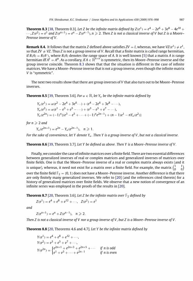
P.N. Shivakumar, K.C. Sivakumar / Linear Algebra and its Applications 430 (2009) 976–998 987
Theorem 8.3 [38, Theorem 0.3]. Let Z be the infinite matrix defined by Z(e1) = e4 − 2e6 + 3e8 − 4e10 +· · ·, Z(e2) = e1 and Z(en+1) = en − Z(en−1),n � 2. Then Z is not a classical inverse of V but Z is a Moore–
Penrose inverse of V .
Remark 8.4. It follows that the matrix Z defined above satisfies ZV = I, whereas, we have VZ(e1) /= e1,
so that ZV /= VZ . Thus Z is not a group inverse of V . Recall that a finite matrix is called range hermitian,
if R(A) = R(A∗), where R(A) denotes the range space of A. It is well known [5] that a matrix A is range
hermitian iff A† = A#. As a corollary, if A ∈ Rn×nis symmetric, then its Moore–Penrose inverse and the
group inverse coincide. Theorem 8.3 shows that that the situation is different in the case of infinite
matrices.We have aMoore–Penrose inverse that is not a group inverse, even though the infinitematrix
V is “symmetric”.
The next two results show that there are group inverses of V that also turn out to beMoore–Penrose
inverses.
Theorem 8.5 [39, Theorem 3.6]. For α ∈ R, let Yα be the infinite matrix defined by
Yα(e1) = α(e2 − 2e4 + 3e6· · ·) + (e4 − 2e6 + 3e8 − · · ·),Yα(e2) = α(e1 − e3 + e5 − · · ·) + (e3 − e5 + e7 − · · ·),Yα(e2n) = (−1)n{(e3 − e5 + · · · + (−1)ne2n−1) + (n − 1)e1 − nYα(e2)}
for n � 2 and
Yα(e2n+1) = e2n − Yα(e2n−1), n � 1.
For the sake of convenience, let Y denote Yα. Then Y is a group inverse of V , but not a classical inverse.
Theorem 8.6 [39, Theorem 3.7]. Let Y be defined as above. Then Y is a Moore–Penrose inverse of V .
Finally,weconsider thecaseof infinitematricesoverafinitefield. Thereare twoessentialdifferences
between generalized inverses of real or complex matrices and generalized inverses of matrices over
finite fields. One is that the Moore–Penrose inverse of a real or complex matrix always exists (and it
is unique), whereas, it need not exist for a matrix over a finite field. For example, the matrix(1 10 0
)over the finite fieldF2 = {0, 1} does not have aMoore–Penrose inverse. Another difference is that there
are only finitely many generalized inverses. We refer to [20] (and the references cited therein) for a
history of generalized matrices over finite fields. We observe that a new notion of convergence of an
infinite series was employed in the proofs of the results in [20].
Theorem 8.7 [20, Theorem 3.6]. Let Z be the infinite matrix over F2 defined by
Z(e1) = e4 + e8 + e12 + · · ·, Z(e2) = e1
and
Z(en+1) = en + Z(en−1), n � 2.
Then Z is not a classical inverse of V nor a group inverse of V , but Z is a Moore–Penrose inverse of V .
Theorem 8.8 [20, Theorems 4.6 and 4.7]. Let Y be the infinite matrix defined by
Y(e1) = e4 + e8 + e12 + · · ·,Y(e2) = e3 + e5 + e7 + · · ·,Y(e2n) =
{e2n+1 + e2n+3 + e2n+5 + · · · if n is odd
e1 + e3 + · · · + e2n−1 if n is even

988 P.N. Shivakumar, K.C. Sivakumar / Linear Algebra and its Applications 430 (2009) 976–998
for n � 2 and
Y(e2n+1) = e2n + Y(e2n−1) for n � 1.
Then Y is a group inverse of V , a Moore–Penrose inverse of V , but not a classical inverse of V .
9. Applications
9.1. Digital circuit dynamics
Weconsider a realweaklyd.d.matrixAandestablishupperand lowerbounds for theminimal eigen-
valueofA, and its correspondingeigenvector, and for theentriesof inverseofA. The results areapplied to
find meaningful two-sided bounds for both �1-norm and the weighted Perron-Norms of the solution
x(t) to the linear differential system x = −Ax, x(0) = x0 > 0. These systems occur in R–C electrical
circuits and a detailed analysis of a model for the transient behavior of digital circuits is given in [36].
We consider J and N as defined in section 2.1, where A is an n × nmatrix with the conditions
D(1): For all i, j ∈ N, with i /= j, aij � 0 and aii > 0.
D(2): For all i ∈ N, |aii| �∑
j /=i |aij| and J /= ∅.D(3): A is irreducible.
Under the conditions D(1)–D(3) and ˙x = −Ax, x(0) = 0, it is proved that for all t � 0,
n∑i=1
xi(t) = e−qtn∑
i=1
zix0,i, (9.1)
where q = q(A) and z = (z1, z2, . . . , zn)T is the positive eigenvector of AT corresponding to q.
The following inequalities also hold:
zmin
zmax‖x0‖1e−qMt � ‖x(t)‖1 � zmax
zmin‖x0‖1e−qmt , (9.2)
where zmin � zi � zmax for all i = 1, 2, . . . ,n. In connectionwith digital circuits, we have the following:
If v = (v1(t), . . . , vn(t))T denotes the vector of node voltages, then the transient evolution of an R-C
circuit (under certain conditions) is described by the equation
Cdv(t)
dt= −Gv + J, (9.3)
where C is a diagonal matrix, J is a given vector and G is a given matrix of conductances. The crucial
performance of the digital circuit is the high operating speed that is measured by the quantity
T(ε) = sup
{t : ‖x(t)‖
‖x0‖ = ε
}. (9.4)
It can be shown that [34] the following inequalities (as a consequence of the inequalities above) hold:
zmin
zmaxe−qMT1 � ε = ‖x(T1(ε))‖1
‖x0‖1 � zmax
zmine−qmT1 (9.5)
for a fixed value T1. This implies that
1
qMln
zmin
εxmax� T1(t) � 1
qmln
zmax
εzmin. (9.6)
9.2. Conformal mapping of doubly connected regions
Solution of a large number of problems in modern technology, such as leakage of gas in a graphite
brick of a gas-cooled nuclear reactor, analysis of stresses in solid propellant rocket grain, simultaneous
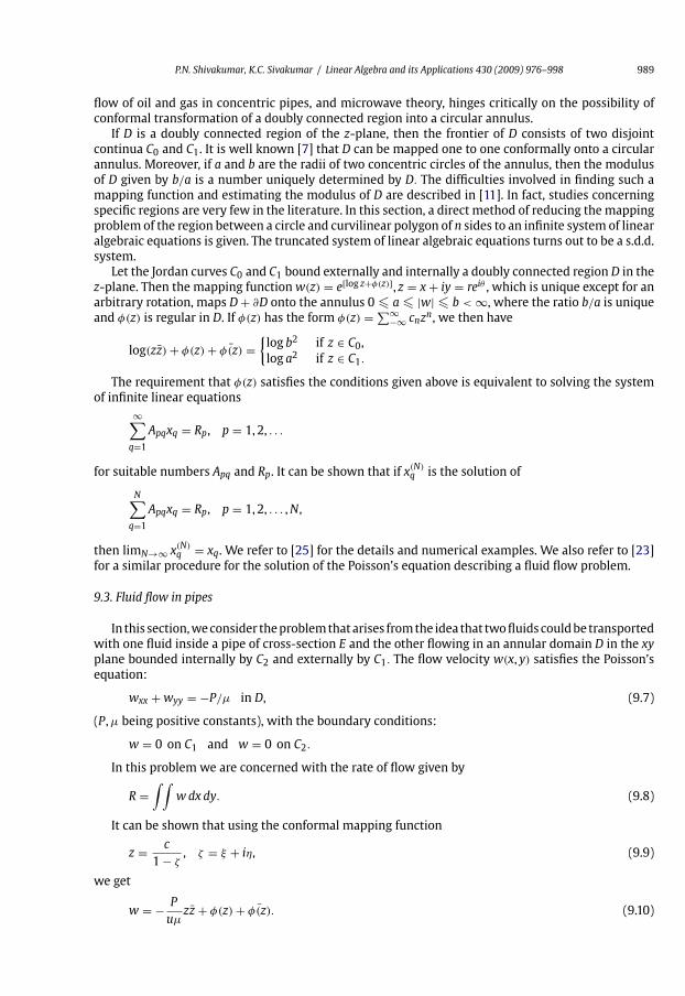
P.N. Shivakumar, K.C. Sivakumar / Linear Algebra and its Applications 430 (2009) 976–998 989
flow of oil and gas in concentric pipes, and microwave theory, hinges critically on the possibility of
conformal transformation of a doubly connected region into a circular annulus.
If D is a doubly connected region of the z-plane, then the frontier of D consists of two disjoint
continua C0 and C1. It is well known [7] that D can be mapped one to one conformally onto a circular
annulus. Moreover, if a and b are the radii of two concentric circles of the annulus, then the modulus
of D given by b/a is a number uniquely determined by D. The difficulties involved in finding such a
mapping function and estimating the modulus of D are described in [11]. In fact, studies concerning
specific regions are very few in the literature. In this section, a direct method of reducing themapping
problem of the region between a circle and curvilinear polygon of n sides to an infinite system of linear
algebraic equations is given. The truncated system of linear algebraic equations turns out to be a s.d.d.
system.
Let the Jordan curves C0 and C1 bound externally and internally a doubly connected region D in the
z-plane. Then the mapping functionw(z) = e[log z+φ(z)], z = x + iy = reiθ , which is unique except for an
arbitrary rotation, maps D + ∂D onto the annulus 0 � a � |w| � b < ∞, where the ratio b/a is unique
and φ(z) is regular in D. If φ(z) has the form φ(z) = ∑∞−∞ cnz
n, we then have
log(zz) + φ(z) + ¯φ(z) ={log b2 if z ∈ C0,
log a2 if z ∈ C1.
The requirement that φ(z) satisfies the conditions given above is equivalent to solving the system
of infinite linear equations
∞∑q=1
Apqxq = Rp, p = 1, 2, . . .
for suitable numbers Apq and Rp. It can be shown that if x(N)q is the solution of
N∑q=1
Apqxq = Rp, p = 1, 2, . . . ,N,
then limN→∞ x(N)q = xq. We refer to [25] for the details and numerical examples. We also refer to [23]
for a similar procedure for the solution of the Poisson’s equation describing a fluid flow problem.
9.3. Fluid flow in pipes
In this section,weconsider theproblemthatarises fromthe idea that twofluidscouldbe transported
with one fluid inside a pipe of cross-section E and the other flowing in an annular domain D in the xy
plane bounded internally by C2 and externally by C1. The flow velocity w(x, y) satisfies the Poisson’s
equation:
wxx + wyy = −P/μ in D, (9.7)
(P,μ being positive constants), with the boundary conditions:
w = 0 on C1 and w = 0 on C2.
In this problem we are concerned with the rate of flow given by
R =∫ ∫
wdx dy. (9.8)
It can be shown that using the conformal mapping function
z = c
1 − ζ, ζ = ξ + iη, (9.9)
we get
w = − P
uμzz + φ(z) + ¯φ(z). (9.10)

990 P.N. Shivakumar, K.C. Sivakumar / Linear Algebra and its Applications 430 (2009) 976–998
We get an infinite series expression for w whose coefficients satisfy an infinite system of algebraic
equations. These equations have been shown to have a unique solution. We refer to [23,27,31] for the
details. In these the following cases are considered.
(a) C0 and C1 being eccentric circles.
(b) C0 and C1 being confocal ellipses.
(c) C0 being a circle and C1 being an ellipse.
(d) C0 and C1 being two ellipses.
Calculation of the rate of the flow suggests that the flow is a maximum when the inner boundary
has the least parameter and the outer boundary has the largest perimeter for a given area of flow.
We refer to [14] for an application of the ideas given above in studying fluid flow in a pipe system
where the insideof theouterpipehasa liningofporousmedia. Thishasbeenshowntohaveapplications
in the cholesterol problem in arteries [14].
9.4. Mathieu equation
Here we consider a Mathieu equation (also see Section 7)
d2y
dx2+ (λ − 2q cos 2x)y = 0 (9.11)
for a given q with the boundary conditions: y(0) = y(π/2) = 0. Our interest is in the case when two
consecutive eigenvalues merge and become equal for some values of the parameter q. This pair of
merging points is called a double point for that value of q. It is well known that for real double points
to occur, the parameter q must attain some pure imaginary value. In [37], the authors developed an
algorithm to compute some special double points. Theoretically, the method can achieve any required
accuracy. We refer to [37] for the details. We briefly present the main results, here.
Using an even solution of the form y(x) = ∑∞r=1 xrq
−r sin 2rx, the Mathieu equation is equivalent
to the system of infinite linear algebraic equations given by Bx = λx, where B = (bij) is an infinite
tridiagonal matrix given by
bij =⎧⎨⎩
−Q if j = i − 1, i � 2,
4i2 if j = i,
1 if j = i + 1, i � 1.
Here Q = −λ2 > 0. Then we have the following result.
Theorem 9.1 [37, Theorem 3.1]. There exists a unique double point in the interval [4, 17].
It is also shown that there is no double point in the interval [17, 37] [37, Theorem 4.1]. They also
present an algorithm for computing the double points. In fact, we have λ ≈ 11.20,Q ≈ 48.09.
The problem of determining the bounds for the width of the instability intervals in the Mathieu
equation has also been studied [33]. We present the main result, here. We consider the following
Boundary Conditions: y′(0) = y′(π/2) = 0, and y(0) = y(π/2) = 0, with the corresponding eigenvalues
denoted by {a2n}∞0 and {b2n}∞0 , respectively. In this connection, the following inequalities are well
known. a0 < b1 < a1 < b2 < a2 < b3 < a3 < · · ·. We give upper and lower bound for a2n − b2n.
Theorem 9.2 [33, Theorem 2]. For n � max{h2+12
, 3},
a2n − b2n � 8h4n
42n[(2n − 1)!]2k−(9.12)
and
a2n − b2n � 8h4n
42n[(2n − 1)!]2k+
[1 − h4
8(2n − 1 − h2)2
], (9.13)

P.N. Shivakumar, K.C. Sivakumar / Linear Algebra and its Applications 430 (2009) 976–998 991
where
k± =(1 ± 3h2
4n2
)n−1∏k=1
(1 ± 3h2
4n2 − 4k2
)2
.
9.5. Bessel’s equation
The Bessel functions, Jn(x), satisfy the well-known recurrence relation:
Jn+1(x) = 2n
xJn(x) − Jn−1(x), n = 0, 1, 2, . . . , 0 < x < 2.
Treating J0(x) as given and solving for Jn(x) = xn,n = 1, 2, . . ., we get a system of equations satisfying
(the conditions considered in Section 6): IM(1), IM(3) and IM(4), and will satisfy IM(2) iff 0 < x < 2.
For instance, choosing x = 0.6, yields the following system of equations:
10x1 − 3x2 = 3J0(0.6),
−3xn−1 + 10nxn − 3xn + 1 = 0, n � 2,
where 3J0(0.6) 2.73601459 [1]. From Corollary 6.3, Section 6, it can be verified that
‖x − x(p,n)‖ �{3
7(0.3)(p+12) + 9
49(n + 1)
}J0(0.6).
Thus for an error of less than 0.01, we choose n = 16 and p = 6. For the purpose of comparison, if
we take p = 16, then for instance we have the following: 9.99555051E−07 as against 9.9956E−07
in [1] and 9.99555051E−07 as against 9.9956E−07 in [1] for J6(0.6) and 1.61393490E−12 as against
1.61396824E−12 in [1] for J10(0.6).Werefer to [29] formoredetails andcomparisonwithknownresults.
9.6. Vibrating membrane with a hole
In this section, we discuss the behaviour of theminimal eigenvalue λ of the Dirichlet Laplacian in an
annulus. LetD1 beadisconR2,withoriginat thecenter, of radius1,D2 ⊂ D1 beadiscof radiusa < 1, the
center (h, 0)ofwhich isatadistanceh fromtheorigin. Letλ(h)denote theminimumDirichleteigenvalue
of the Laplacian in the annulus D := Dh := D1\D2. The following conjecture is proposed in [19]:
Conjecture. The minimal eigenvalue λ(h) is a monotonic decreasing function of h on the interval 0 � h �(1 − a). In particular, λ(0) > λ(h),h > 0.
The above conjecture is supported by the following lemmas.
Lemma 9.3. We have
dλ
dh=∫Su2NN1ds,
where N is the unit normal to S = Sh, pointing into the annulus Dh,N1 is the projection of N onto x1-axis,uNis the normal derivative of u, and u(x) = u(x1, x2) is the normalized L2(D) eigenfunction corresponding to
the first eigenvalue λ.
Let D(r) denote the disc |x| � r and μ(r) be the first Dirichlet eigenvalue of the Laplacian in D1\Dr .
Then we have,
Lemma 9.4. μ(a − h) < λ(h) < μ(a + h), 0 < h < 1 − a.
The conjecture is also substantiated by numerical results. For details we refer to [19].

992 P.N. Shivakumar, K.C. Sivakumar / Linear Algebra and its Applications 430 (2009) 976–998
9.7. Groundwater flow
Here, we are concerned with the problem of finding the hydraulic head, φ, in a non-homogeneous
porous medium, the region being bounded between two vertical impermeable boundaries, bounded
on top by a sloping sinusoidal curve and unbounded in depth. The hydraulic conductivity K(z) is
modelled as K(z) = edz , supported by some data available from Atomic Energy of Canada Ltd. We
develop a method that reduced the problem to that of solving an infinite system of linear equations.
The present method yields a Grammian matrix which is positive definite, and the truncation of this
system yields an approximate solution that provides the best match with the given values on the top
boundary. We refer to [36] for the details. We only present a brief outline, here.
We require φ to satisfy the equation:
∇ · (edz∇φ(x, z)) = 0,
where ∇ is the vector differential operator
i∂
∂x+ j
∂
∂z.
The domain under consideration is given by
0 < x < L, −∞ < z < g(x) = −[ax
L+ V sin
(2πnx
L
)], (9.14)
where d � 0, L � 0, a � 0 and V are constants and n is a positive integer. The boundary conditions are
given by
∂φ
∂x
∣∣∣∣x=0
= ∂φ
∂x
∣∣∣∣x=L
= 0, (9.15)
φ(x, z) is bounded on z � g(x), and φ(x, z) = z on z = g(x). The determination of φ reduces to the
problem of solving the infinite system of linear algebraic equations:
∞∑m=0
bkmαm = ck , k = 0, 1, 2, . . . , (9.16)
where bkm are given by means of certain integrals. The infinite matrix B = (bkm) is the Grammian of a
set of functions which arise in the study. The numbers bkm become difficult to evaluate for large values
of k and m by numerical integration. The authors use an approach using modified Bessel functions,
which gives analytical expressions for bkm. They also present numerical approximations and estimates
for the error.
9.8. Semi-infinite linear programming
Infinite linear programming problems are linear optimization problems where, in general there
are infinitely (possibly uncountable) many variables and constraints related linearly. There are many
problems arising from real world situations that can be modelled as infinite linear programs. The
bottleneck problemof Bellman in economics, infinite games, continuous network flows, to name a few.
We refer to the excellent book [2] for anexpositionof infinite linear programs, a simplex typemethodof
solutionandapplications. Semi-infinite linearprogramsareasubclassof infiniteprograms,wherein the
number of variables is finite with infinitely many constraints in the form of equations or inequalities.
Semi-infinite programs have been shown to have applications in a number of areas that include robot
trajectory planning, eigenvalue computations, vibrating membrane problems and statistical design
problems. Formore detailswe refer to the two excellent reviews [10,18] on semi-infinite programming.
Let us recall that a vector space V is said to be partially ordered if there is a relation denoted ‘�’
defined on V that satisfies reflexivity, antisymmetry and transitivity andwhich is also compatiblewith
the vector space operations of addition and scalar multiplication. Let H1 and H2 be real Hilbert spaces
with H2 partially ordered, A : H1 → H2 be bounded linear, c ∈ H1 and a, b ∈ H2 with a � b. Consider
the linear programming problem called interval linear program ILP(a, b, c,A) :

P.N. Shivakumar, K.C. Sivakumar / Linear Algebra and its Applications 430 (2009) 976–998 993
Maximize 〈c, x〉subject to a � Ax � b.
Such problems were investigated by Ben–Israel and Charnes [4] in the case of finite dimensional
real Euclidean spaces and explicit optimal solutionswere obtained using the techniques of generalized
inverses of matrices. These results were later extended to the general case and several algorithms
were proposed for interval linear programs. Some of these results were extended to certain infinite
dimensional spaces [12,13].
The objective of this section is to present an algorithm for the countable semi-infinite interval linear
program denoted SILP(a, b, c,A) of the type:
Maximize 〈c, x〉subject to a � Ax � b,
where c ∈ Rm,H, a real separable partially orderedHilbert space, a, b ∈ Hwith a � b and A : Rm −→ H
is a (bounded) linear map. Finite dimensional truncations of the above problems are solved as finite
dimensional interval programs. This generates a sequence {xk} with each xk being optimal for the
truncated problem at the kth stage. This sequence is shown to converge to an optimal solution of the
problem SILP(a, b, c,A). We also show how this idea can be used to obtain optimal solutions for con-
tinuous semi-infinite linear programs and to obtain approximate optimal solutions to doubly infinite
interval linear programs.
Wewill quickly go through thenecessary definitions and results needed for proving ourmain result.
We will state our results generally and then specialize later. Let H1 and H2 be real Hilbert spaces with
H2 partially ordered, A : H1 → H2 be linear, c ∈ H1 and a, b ∈ H2 with a � b. Consider the interval linear
program ILP(a, b, c,A) :
Maximize 〈c, x〉subject to a � Ax � b.
Definition 9.5. Set F = {x : a � Ax � b}. A vector x∗ is said to be feasible for ILP(a, b, c,A) if x∗ ∈ F . The
problem ILP(a, b, c,A) is said to be feasible if F /= ∅. A feasible vector x∗ is said to be optimal if 〈c, (x∗ −x)〉 � 0 for every x ∈ F . ILP(a, b, c,A) is said to be bounded if sup{〈c, x〉 : x ∈ F} < ∞. If ILP(a, b, c,A) is
bounded, then the value α of the problem is defined as α = sup{〈c, x〉 : x ∈ F}.
Wewill assume throughout the paper that F /= ∅. Boundedness is then characterized by Lemma 9.6,
to follow. Let A : H1 −→ H2 be linear. A linear map T : H2 −→ H1 is called a {1}-inverse of A if ATA = A.
We recall that A bounded linear map A has a bounded {1}-inverse iff R(A), the range space of A is
closed [16].
Lemma 9.6 [12, Lemma 2]. Suppose H1 and H2 are real Hilbert spaces,H2 is partially ordered and
ILP(a, b, c,A) is feasible. If ILP(a, b, c,A) is bounded then c ⊥ N(A). The converse holds if A has a bounded
{1}-inverse and [a, b] = {z ∈ H2 : a � z � b} is bounded.
9.9. Finite dimensional approximation scheme
Let H be a partially ordered real Hilbert space with an orthonormal basis {un : n ∈ N} such that
un ∈ C∀n, where C is the positive cone in H. Let {Sn} be a sequence of subspaces in H such that
{u1,u2, . . . ,un} is an orthonormal basis for Sn. Then ∪∞n=1
Sn = H. Let Tn : H −→ H be the orthogonal
projection of H onto Sn. Then for x = (x1, x2, . . .) ∈ H, Tn(x) = (x1, x2, . . . , xn, 0, 0, . . .). Then the sequence
{Tn} converges strongly to the identity operator on H.

994 P.N. Shivakumar, K.C. Sivakumar / Linear Algebra and its Applications 430 (2009) 976–998
Consider thesemi-infinite linearprogramSILP(a, b, c,A).Wewill assumethat thisproblemisbounded
and that the columns of A are linearly independent. Then SILP(a, b, c,A) is bounded, by Lemma 9.6.
Define the kth subproblem SILP(Tka, Tkb, c, TkA) denoted by SILPk by
Maximize 〈c, x〉subject to Tka � TkAx � Tkb.
SILPk has k interval inequalities in the m unknowns xi, i = 1, 2, . . . ,m. In view of the remarks given
above, it follows that SILP(Tka, Tkb, c, TkA) is bounded whenever k � m.
We now state a convergence result for the sequence of optimal solutions of the finite dimensional
subproblems. The proof will appear elsewhere [40].
Theorem 9.7. Let {xk} be a sequence of optimal solutions for SILPk. Then {xk} converges to an optimal
solution of SILP(a, b, c,A).
We next present a simple example to illustrate Theorem 9.7. A detailed study of various exam-
ples showing how the above theorem can be used to obtain optimal solutions even for a continuous
semi-infinite linear program, is presently underway [40].
Example. Let H = �2, A : R2 → �2 be defined by
A =
⎛⎜⎜⎜⎜⎜⎜⎝
1 0
1 112
14
13
19
.
.
....
⎞⎟⎟⎟⎟⎟⎟⎠a =
(0,−1,− 1
4,− 1
9, . . .
), b = (1, 0, 0, . . .)and c = (1, 0). Consider thesemi-infiniteprogramSILP(a, b, c,A)
given by
Maximize x1subject to 0 � x1 � 1,−1k2
� x1k
+ x2k2
� 0, k = 1, 2, 3, . . .
Clearly c ⊥ N(A), asN(A) = {0} and so the problem is bounded, by Lemma 9.6. Rewriting the second
set of inequalities, we get
−1
k� x1 + x2
k� 0, k = 1, 2, 3, . . .
Thenx1 = 0,bypassing to limitask → ∞. Thus (0,α),−1 � α � 0 isanoptimal solution forSILP(a, b, c,A)
with optimal value 0.
Nowwe consider the finite truncations. Let Sk = {e1, e2, . . . , ek} where {e1, e2, e3, . . .} is the standard
orthonormal basis for �2. Define Tk =(Ik 00 0
)where Ik is the identity map of order k × k, k � 2. Thus
R(TkA) = Sk . The subproblem SILP(Tka, Tkb, c, TkA) is
Maximize x1
subject to 0 � x1 � 1,
−1
(l − 1)2� x1
l − 1+ x2
(l − 1)2� 0, l = 2, 3, . . . , k.

P.N. Shivakumar, K.C. Sivakumar / Linear Algebra and its Applications 430 (2009) 976–998 995
Clearly, the subproblem SILP(Tka, Tkb, c, TkA) is bounded and the optimal solution is xk =(
1k−2
, −(k−1)
k−2
).
This converges to (0,−1) in the limit as k → ∞.
9.10. Approximate optimal solutions to a doubly infinite linear program
In this section, we show how we can obtain approximate optimal solutions to continuous infinite
linear programming problems. With the notations earlier, assume that ILP(a, b, c,A) is bounded. Let
ck denote the vector in H whose first k components are the same as the vector c and whose other
components are zero. Let Ak denote the matrix with k columns and infinitely many rows whose k
columns are precisely the same as the first k columns of A. Consider the problem:
Maximize 〈ck ,u〉subject to a � Aku � b
for u ∈ Rk. This problem is SILP(a, b, ck ,Ak) for each k. Suppose that the columns of Ak are linearly
independent for all k. Denoting SILP(a, b, ck ,Ak) by Pk , we solve Pk using Theorem 9.7. This gener-
ates a sequence {uk}. Let uk = (u1,u2, . . . ,uk)T be an optimal solution for Pk . Let u = (uk , 0)T . Then
Ak+1u = Akuk . Since a � Anu
k � b, u is feasible for Pk+1. Let v(Pk) denote the value of problem Pk , viz.,
v(Pk) := sup{〈ck ,u〉 : a � Aku � b.} Then v(Pk+1) � v(Pk) as 〈ck+1,u〉 � 〈ck ,u〉. Let xk = (uk , 0, 0 · · ·) ∈ H.
Then xk is feasible for ILP(a, b, c,A) and 〈c, xk〉 = 〈ck , xk〉, the value of Pk . Thus the sequence {〈c, xk〉}is an increasing sequence bounded above by the value of ILP(a, b, c,A) and is hence convergent. It
follows that xk is weakly convergent. However, unlike the semi-infinite case, it need not be con-
vergent. (In the following example, it turns out that xk is convergent.) So, we have optimal value
convergence but not optimal solution convergence. Hence our method yields only an approximate
optimal solution for a continuous linear program. It will be interesting to study how good is this
approximation.
Example. Let A : �2 → �2 be defined by A =
⎛⎜⎜⎜⎝1 0 0 0
1 12
0 · · ·1 1
213
· · ·...
.
.
.
.
.
.. . .
⎞⎟⎟⎟⎠. Let c =(1, 1
4, 19, . . .
), a = 0 and b =
(1, 1
2, 13, . . .
). The problem ILP(a, b, c,A) is
Maximize x1 + x24
+ x39
+ · · ·
subject to 0 �l∑
i=1
xii
� 1
l, l = 1, 2, 3, . . . .
Clearly A ∈ BL(�2) and N(A) = {0}. Therefore c ⊥ N(A), i.e., the problem ILP(a, b, c,A) is bounded. Con-
sider the kth subproblem Pk:
Maximize 〈ck ,u〉subject to a � Aru � b, r = 1, 2, . . . , k,
where ck = (1, 1/4, 1/9, . . . , 1/k2), and Ak : Rk → �2 is defined by A =
⎛⎜⎜⎜⎜⎜⎜⎝
1 0 · · · 0
1 12
· · · · · ·...
.
.
. · · ·...
1 12
· · · 1k
.
.
.
.
.
. · · ·...
⎞⎟⎟⎟⎟⎟⎟⎠. Clearly, the
subproblem is bounded. By thefinite dimensional scheme, the optimal solution of the subproblem Pk is

996 P.N. Shivakumar, K.C. Sivakumar / Linear Algebra and its Applications 430 (2009) 976–998
found to be xk =(1,−1,− 1
2,− 1
3, . . . ,− 1
k−1
)which converges to x∗ =
(1,−1,− 1
2,− 1
3, . . .
). The optimal
value converges to 6.450. We conclude by observing that since A is invertible, it is possible to solve the
original problem by the methods in [12], directly.
9.11. Eigenvalues of the Laplacian on an elliptic domain
The importance of eigenvalue problems concerning the Laplacian is well documented in classical
and modern literatures. Finding the eigenvalues for various geometries of the domains has posed
many challengeswhich have included infinite systems of algebraic equations (see Section 9.4), asymp-
totic methods, integral equations,finite element methods, etc. Details of earlier work can be found in
[44]. The eigenvalue problems of the Laplacian is represented by the Helmholtz equations, Telegraph
equations or the equations of the vibrating membrane and is given by
∂2u
∂x2+ ∂2u
∂y2+ λ2u = 0 in D,
u = 0 on ∂D,
where D is a plane region bounded by smooth curve ∂D. The eigenvalue kn and corresponding eigen-
functions un describe the natural modes of vibration of a membrane. According to the maximum
principle, kn must be positive for a nontrivial solution to exist. Further kn,n = 1, 2, . . . are ordered
satisfying
0 < k1 < k2 < · · · < kn < · · ·Using complex variables z = x + iy, z = x − iy, the problem becomes
∂2u
∂z∂ z+ λ2
4u = 0 in D and u = 0 on C (9.17)
and u = u(z, z), It is well known that the general solution to (9.17) is given by
u ={f0(z) −
∫ z
0f0(t)
∂
∂tJ0
(λ√z(z − t)
)dt
}+ conjugate, (9.18)
where f0(z) is an arbitrary holomorphic function which can be expressed as
f0(z) =∞∑n=0
anzn, (9.19)
J0 is the Bessel’s function of the first kind of order 0, which is given by a series representation as,
J0
(λ√z(z − t)
)=
∞∑k=0
(−λ2
4
)kzk(z − t)k
k!k! . (9.20)
On substituting for f0(z) in the general solution, we get the general solution to the Helmholtz equation
as given by
u = 2a0J0(λ√zz)
+∞∑n=1
∞∑k=0
An,k
⎛⎝(z + z)n +n/2∑m=1
(−1)mn
m
(n − m − 1
m − 1
)(z + z)n−2m(zz)man
⎞⎠ (zz)k.
demonstrating that the general solution of (9.17) without boundary conditions can be expressed in
terms of power of zz and (z + z).
In our case, we consider the domain bounded by the ellipse represented by
x2
α2+ y2
β2= 1,

P.N. Shivakumar, K.C. Sivakumar / Linear Algebra and its Applications 430 (2009) 976–998 997
which can be expressed correspondingly in the complex plane by
(z + z)2 = a + bzz, (9.21)
where a = 4α2β2
β2−α2 , b = 4α2
α2−β2 .
After considerable manipulation, we get the value of u on the ellipse as,
u = 2a0 +∞∑n=1
A2n,0b0,nan
+∞∑k=1
(−λ2
4
)k2a0k!k! (zz)
k
+∞∑k=1
⎡⎣ k∑n=1
⎛⎝A2n,kb0,n +n∑
l=1
A2n,k−lbl,n
⎞⎠ an
⎤⎦ (zz)k
+∞∑k=1
⎡⎣ ∞∑n=k+1
⎛⎝A2n,kb0,n +k∑
l=1
A2n,k−lbl,n
⎞⎠ an
⎤⎦ (zz)k , (9.22)
For u = 0 on the elliptic boundary, we equate the powers of zz to zero where we arrive at an infinite
system of linear equations of the form
∞∑k=0
dknan = 0, n = 0, 1, 2, . . . ∞, (9.23)
where dkn’s are know polynomials of λ2. In [44], the infinite system is truncated to n × n system and
numerical vaues were calculate and compared to existing results in literature. The method derived
here provides a procedure to numerically calculate the eigenvalues.
Acknowledgements
The authors thank the referee for suggestions and comments that led to a vastly improved presen-
tation of the original version. The second author thanks the first author for inviting him to Winnipeg
during the summer of 2004.
References
[1] M. Abramovitz, I. Stegun, Handbook of Mathematical Functions, Dover, New York, 1965.[2] E.J. Anderson, P. Nash, Linear Programming in Infinite Dimensional Spaces, John Wiley, New York, 1987.[3] R. Bellman, Matrix Analysis, McGraw Hill, 1970.[4] A. Ben-Israel, A. Charnes, An explicit solution of a special class of linear programming problems, Oper. Res. 16 (1968)
1166–1175.[5] A. Ben-Israel, T.N.E. Greville, Generalized Inverses: Theory and Applications, second ed., Springer-Verlag, New York, 2003.[6] M. Bernkopf, A history of infinite matrices, Arch. Hist. Exact Sci. 4 (1968) 308–358.[7] C. Caratheodory, Theory of Functions of a Complex Variable, vol. 2, Chelsea Pub. Co., New York, 1954.[8] M.M. Chawla, P.N. Shivakumar, A finite difference method for a class of two-point boundary value problems over a
semi-infinite range, J. Comput. Appl. Math. 15 (1986) 251–256.[9] R.G. Cooke, Infinite Matrices and Sequence Spaces, Dover, New York, 1955.
[10] R. Hettich, K.O. Kortanek, Semi-infinite programming: theory, methods and applications, SIAM Rev. 35 (1993) 380–429.[11] L.V. Kantorovich, V.I. Krylov, Approximate Methods of Higher Analysis, Interscience, New York, 1964.[12] S.H. Kulkarni, K.C. Sivakumar, Applications of generalized inverses to interval linear programs in Hilbert spaces, Numer.
Funct. Anal. Optim. 16 (7,8) (1995) 965–973.[13] S.H. Kulkarni, K.C. Sivakumar, Explicit solutions of a special class of linear programming problems in Banach spaces, Acta
Sci. Math. (Szeged) 62 (1996) 457–465.[14] M. Luca, S. Kocabiyik, P.N. Shivakumar, Flow past and through a porous medium in a doubly connected region,Appl. Math.
Lett. 11 (2) (1998) 49–54.[15] A.M. Ostrowski, On some conditions for nonvanishing of determinants, Proc. Amer. Math. Soc. 12 (1961) 268–273.[16] M.Z. Nashed (Ed.), Generalized Inverses and Applications, Academic Press, New York, 1974[17] M.Z. Nashed, G.F. Votruba, A unified operator theory of generalized inverses, in: [15], pp. 1–109.

998 P.N. Shivakumar, K.C. Sivakumar / Linear Algebra and its Applications 430 (2009) 976–998
[18] E. Polak, On the mathematical foundations of nondifferentiable optimization in engineering design, SIAM Rev. 29 (1987)21–89.
[19] A.G. Ramm, P.N. Shivakumar, Inequalities for the minimal eigenvalue of the Laplacian in an annulus, Math. Ineq. Appl. 1(4) (1998) 559–563.
[20] C.R. Saranya, K.C. Sivakumar, Generalized inverses of invertible infinitematrices over a finite field,Linear Algebra Appl. 418(2006) 468–479.
[21] P.N. Shivakumar, Diagonally dominant infinite matrices in linear equations, Util. Math. 1 (1972) 235–248.[22] P.N. Shivakumar, R. Wong, Linear equations in infinite matrices, Linear Algebra Appl. 7 (1) (1973) 553–562.[23] P.N. Shivakumar,Viscousflowinpipeswhosecross-sectionsaredoubly connected regions,Appl. Sci. Res. 27 (1973)355–365.[24] P.N. Shivakumar, K.H. Chew, A sufficient condition for nonvanishing of determinants, Proc. Amer. Math. Soc. 43 (1) (1974)
63–66.[25] P.N. Shivakumar, K.H. Chew, On the conformal mapping of a circular disc with a curvilinear polygonal hole,Proc. Ind. Acad.
Sci. 85 A (6) (1977) 406–414.[26] P.N. Shivakumar, K.H. Chew, J.J.Williams, Error bounds for the truncation of infinite linear differential systems,J. Inst.Math.
Appl. 25 (1980) 37–51.[27] P.N. Shivakumar, K.H. Chew, On solutions of Poisson’s equation for doubly connected regions, Pusat Pengajan Sains
Matematik, University Sains Malaysia, Tech. Rep., 1982, 2/82.[28] P.N. Shivakumar, J.J. Williams, N. Rudraiah, Eigenvalues for infinite matrices, Linear Algebra Appl. 96 (1987) 35–63.[29] P.N. Shivakumar, J.J. Williams, An iterative method with truncation for infinite linear systems, J. Comput. Appl. Math. 24
(1988) 199–207.[30] P.N. Shivakumar, I. Leung, On some higher order derivatives of solutions of y′′ + p(x)y = 0, Util. Math. 41 (1992) 3–10.[31] P.N. Shivakumar, C. Ji, On Poisson’s equation for doubly connected regions, Canad. Appl. Math. Quar. 1 (4) (1993) 555–567.[32] P.N. Shivakumar, C. Ji, Upper and lower bounds for inverse elements of finite and infinite tri-diagonal matrices, Linear
Algebra Appl. 247 (1996) 297–316.[33] P.N. Shivakumar, Q. Ye, Bounds for the width of instability intervals in the Mathieu equation, Oper. Theory: Adv. Appl. 87
(1996) 348–357.[34] P.N. Shivakumar, J.J. Williams, Q. Ye, C. Marinov, On two-sided bounds related to weakly diagonally dominantM-matrices
with application to digital circuit dynamics, SIAM J. Matrix Anal. Appl. 17 (2) (1996) 298–312.[35] P.N. Shivakumar, C. Ji, On the nonsingularity of matrices with certain sign patterns, Linear Algebra Appl. 273 (1998) 29–43.[36] P.N. Shivakumar, J.J.Williams, Q. Ye, C. Ji, An analysis of groundwater flow in an infinite regionwith a sinusoidal top,Numer.
Funct. Anal. Optim. 21 (1–2) (2000) 263–271.[37] P.N. Shivakumar, J. Xue, On the double points of a Mathieu equation, J. Comput. Appl. Math. 107 (1999) 111–125.[38] K.C. Sivakumar, Moore–Penrose inverse of an invertible infinite matrix, Linear and Multilinear Algebra 54 (2006) 71–77.[39] K.C. Sivakumar, Generalized inverses of an invertible infinite matrix, Linear and Multilinear Algebra 54 (2006) 113–122.[40] K.C. Sivakumar, J. Mercy Swarna, An algorithm for semi-infinite linear programs, submitted for publication.[41] O. Taussky, A recurring theorem on determinants, Amer. Math. Mon. 56 (1948) 672–676.[42] J.M. Varah, A lower bound for the smallest singular value of a matrix, Linear Algebra Appl. 11 (1975) 3–5.[43] R.S. Varga, Matrix Iterative Analysis, Prentice-Hall, Englewood Cliffs, New Jeresy, 1962.[44] P.N. Shivakumar, Y. Wu, Eigenvalues of the Laplacian on an elliptic domain, Comput. Math. Appl. 55 (2008) 1129–1136.