linear algebra and its applica tions - penn …kazdan/260s12/notes/vectors/strang... · linear...

IIiI,

LINEAR ALGEBRAAND ITS

APPLICATIONSTHIRD EDITION

GILBERT STRANGMassachusetts Institute of Technology

Saunders College PublishingHarcourt Brace Jovanovich College Publishers

Fort Worth Philadelphia San DiegoNew York Orlando Austin San Antonio

Toronto Montreal London Sydney Tokyo

242 4 Determinants

into the identity without becoming singular on the way. (The straight path from Ato I, with a chain A(t) = A + t(I - A), does go from A(O) = A to A(I) = I, but in be-tween A(t) might be singular. The problem is not so easy, and soluti(JDSare welcomedby the author.)

54.18 If A is nonsingular, show that there must be some permutation P for which PA has

no zeros on its main diagonal. It is not the f from elimination.

4.19 Explain why the point (x, y) is on the line through (2, 8) and (4, 7) if

[

XYl

]det281=O,

4 7 1

or x + 2y - 18 = O.

EIGENVALUES ANDEIGENVECTORS

4.20 In analogy with the previousexercise,what is the equation for (x, y, z) to be on theplane through (2, 0, 0), (0, 2, 0), and (0, 0, 4)? It involves a 4 by 4 determinant.

4.21 If the points (x, y, z), (2, 1,0), and (1, I, 1) lie on a plane through the origin, whatdeterminant is zero? Are the vectors (1,0, -I), (2, 1,0), (1, I, 1) dependent orindependent?

4.22 If every row of A has either a single + I, or a single -I, or one of each (and isotherwise zero) show that det A = 1 or -lor O.

4.23 If C = [~ nand D= [~ ~] thenCD= - DC in Exercise 1.4.14 becomes

CD + DC = 0 or

r

2a e b O

J r

U

J r

O

J

b a+d 0 b v = 0 .e 0 a+d e w 0o e b 2dz 0

INTRODUCTION.5.1

r

Ia a2 a3

J

1 b b2 b3V4=det 231 e e e

1 x x2 x3

This chapter begins the "second half" of matrix theory. The first part was almostcompletely involved with linear systems Ax = b, and the fundamentaltechniquewas elimination. From now on row operations will play only a minor role. Thenew problems will still be solved by simplifying a matrix-making it diagonal orupper triangular-but the basic step is no longer to subtract a.muitiple of one rowfrom another. We are not interested any more in preserving the row space of amatrix, but in preserving its eigenvalues. Those are changed by' elimination.

The chapter on determinants was really a transition from the old problemAx = b to the new problem of eigenvalues. In both cases tbe determinant leadsto a "formal solution": to Cramer's rule for x = A-I b and to the polynomialdet(A - AI) whose roots will be the eigenvalues. (We emphasize that all matricesare now square; the eigenvalues of a rectangular matrix make no more sense thanits determinant.) As always, the determinant can actually be used to solve theproblem, if n = 2 or 3. For large n the computation of eigenvalues is a longer andmore difficult task than solving Ax = b, and even Gauss himselfdid not helpmuch. But that can wait.

The first step is to understand what eigenvalues are and how they can be useful.One of their applications, the one by which we want to introduce them, is to thesolution of ordinary differential equations. We shall not assume that the readeris an expert on differential equations! If you can differentiate the usual functionslike x', sin x, and eX,you know enough. As a specific example, consider the coupled

(a) Find the determinant of this 4 by 4 coefficientmatrix A.(b) Show that det A = 0 in two cases: a + d = 0 or ad - be = O.

In all other cases, CD = -DC is only possible with D = O.

4.24 Explain why the 4 by 4 Vandermonde determinant

must be a cubic polynomial in x, and why that polynomial is zero at x = a, x = b,and x = e. Using the cofactor of x3 from Exercise4.2.10leads to

~=~-a~-a~-~x-~x-~x-4

4.25 The circular shift permutes (I, 2, . . . , n) into (2, 3, . . . , 1).What is the correspondingpermutation matrix P, and (depending on n) what is its determinant?

244 5 Eigenvalues and Eigenvectors5.1 Introduction 245

dv

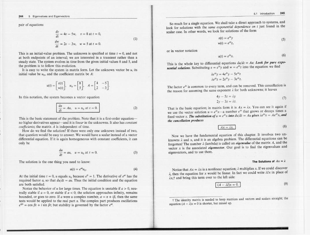
dt = 4v - 5w, v = 8 at t = 0,

dw

at = 2v - 3w, w = 5 at t = O.

So much for a single equation. We shall take a direct approach to systems, andlook for solutions with the same exponential dependence on t just found in thescaJar case. In other words, we look for solutions of the form

pair of equations

(1) v(t) = eA'y

w(t) = e!.'z,(5)

This is an initial-value problem. The unknown is specified at time t = 0, and notat both endpoints of an interval;we are interested in a transient rather than asteady state.The systemevolvesin time from the giveninitial values8 and 5, andthe problem is to follow this evolution.

It is easy to write the system in matrix form. Let the unknown vector be u, itsinitial value be uo, and the coefficient matrix be A:

or in vector notation

u(t) = e!.'x. (6)

[V(t)

J [8

J [4

u(t) = w(t) , Uo= 5 ' A = 2

-5

J-3 .

This is the whole key to differential equations dujdt = Au: Look for pure expo-nential solutions. Substituting v = e!.'y and w = e!.'z into the equation we find

Ae!.'y= 4e!.'y - 5e!.tz

Ae!.'z= 2e!.'y - 3e!.'z.

The factor e!.' is common to every term, and can be removed. This cancellation isthe reason for assuming the same exponent A for both unknowns; it leaves

4y - 5z = AY

2y - 3z = AZ.(7)In this notation, the system becomes a vector equation

I ~ = Au, u = Uoat t = 0.1

This is the basic statement of the problem. Note that it is a first-order equation-no higher derivatives appear-and it is linear in the unknowns. It also has constant

coefficients; the matrix A is independent of time.How do we find the solution? If there were only one unknown instead of two,

that question would be easy to answer. We would have a scalar instead of a vectordifferential equation. If it is again homogeneous with constant coefficients, it canonly be

(2) That is the basic equation; in matrix form it is Ax = Ax. You can see it again ifwe use the vector solution u = e!.'x-a number e!.' that grows or decays times afixed vector x. Thesubstitution ofu = e!.'xintodujdt = Au gives Ae!.'x = Ae!.'x, andthe cancellationproduces

IAx = AX. I (8)

du

dt = au, u = Uoat t = O. (3)

Now we have the fundamental equation of this chapter. It involves two un-knowns A and x, and it is an algebra problem. The differential equations can beforgotten!The number A(lambda)is calledan eigenvalueof the matrix A, and thevector x is the associatedeigenvector.Our goal is to find the eigenvaluesandeigenvectors,and to use.them.

The solution is the one thing you need to know: The Solutionsof Ax =).

u(t) = ea,uo. (4)

At the initial time t = 0, u equals Uo because eO= 1.The derivative of ea'has therequired factor a, so that dujdt = au. Thus the initial condition and the equationare both satisfied.

Notice the behavior of u for large times. The equation is unstable if a > 0, neu-trally stable if a = 0, or stable if a < 0; the solution approaches infinity, remainsbounded, or goes to zero. If a were a complex number, a = (X + ip,then the sametests would be applied to the real part (x.The complex part produces oscillationseiP'= cospt + i sin pt; but stability is governed by the factor ea'.

Notice that Ax = Ax is a nonlinear equation; Amultiplies x. If we could discoverA, then the equation for x would be linear. In fact we could write A.Ix in place ofAX,tand bring this term over to the left side:

I (A - A.I)x = O. I (9)

t 1;he identity matrix is needed to keep matrices and vectors and scalars straight; theequation (A - ),)x = 0 is shorter, but mixed up.

246 5 Eigenvalues and Eigenvectors 5.1 Introduction 247

This is the key to the problem: a nonzero vector x in its nullspace.t In fact the nullspace contains a whole lineof eigenvectors; it is a subspace!

The vector x is in the nul/space of A - ).JThe number Ais chosen so that A - J./ has a nullspace.

Of course every matrix has a nullspace. It was ridiculous to suggest otherwise,but you see the point. We want a nonzero eigenvector x. The vector x = 0 alwayssatisfies Ax = Ax, and it is always in the nulls pace, but it is useless in solving dif-ferential equations. The goal is to build u(t) out of exponentials eAlx,and we areinterested only in those particular values Afor which there is a nonzero eigenvectorx. To be of any use, the nullspaceof A - J./ must contain vectors other thanzero. In short, A - J./ must be singular.

For this, the determinant gives a conclusive test.

The solution (the first eigenvector) is any multiple of

The computation for A2is done separately:

fA The¥ntimb;rxis. aneigenyalt1~f .Ajf .aridohlY;ifI deJ(A+'xl)=O.

IT...

.

.

h...'

.

i'~

.

lS..

.

.

.

.

..

t.

p.

.

.

e.

.

..

.

.cha

.

ra4!";'!k

..

..

.

..

.

e

.

..

.

qU@Ofl~afld e

.

a~

.

h

.

.S~U~iOfl khas;acQfl'esJ?{lfldi1J~~i~~n~

yectorx.: . . . .(A or

~. - -.....

The second eigenvector is any multiple of

In our example,shiftingA by J./ gives

(4 - A)(- 3 - A)+ 10 or

Note on computing eigenvectors: In the 2 by 2 case, both rows of A - J./ will bemultiples of the same vector (a, b). Then the eigenvector is any multiple of ( - b, a).The rows of A - A21were (2, - 5) and the eigenvector was (5, 2). In the 3 by 3 case,I often set a component of x equal to one and solve (A - J./)x = 0 for the othercomponents. Of course if x is an eigenvector then so is 7x and so is - x.All vectorsin the nullspace of A - J./ (which we call the eigenspace)will satisfy Ax = Ax.Inthis case the eigenspaces are the lines through Xl = (1, 1) and X2 = (5, 2).

Before going back to the application (the differential equation), we emphasizethe steps in solving the eigenvalue problem:

[4-A -5

]A-).J= 2 -3-A'

Note that Ais subtracted only from the main diagonal (because it multiplies I). Thedeterminant of A - J./ is

This is the "characteristic polynomial." Its roots, where the determinant is zero,are the eigenvalues. They come from the general formula for the roots of a quad-ratic, or from factoring into A2- 1 - 2 = (A+ 1)(1- 2).That is zero if A= -1or 1 = 2, as the generalformulaconfirms:

A= - b :1:~~2 - 4ac = 1 :1:2J9 = _ 1 or 2.

1. Compute the determinant of A - J./. With 1 subtracted along the diagonal,this determinant is a polynomialof degreen.

2. Find the roots of this polynomial. The n roots are the eigenvalues.3. Foreacheigenvaluesolvetheequation(A - J./)x = O. Since the determinant

is zero, there are solutions other than x = O.Those are the eigenvectors.

There are two eigenvalues, because a quadratic has two roots. Every 2 by 2 matrixA - ).J has 12 (and no higher power) in its determinant.

Each of thesespecialvalues,1 = -1 and 1 = 2, leads to a solutionof Ax = Axor (A - J./)x = O. A matrix with zero determinant is singular, so there must be t If solving (A - 'u)x = 0 leads you to x = 0, then), is not an eigenvalue.


In the differential equation, this produces the special solutions u = eAtx.They arethe pure exponential solutions

his life trying to get in line with the natural frequencies of the market. The eigen-values are the most important feature of practically any dynamical system.

u = eA,txI = e-tGJand

u = eA2tx2= e2tGJSummary and Examples

Writing the two components separately, this means that

v(t) = 3e-t + 5e2t, w(t) = 3e-t + 2e2t.

The initial conditions Vo= 8 and Wo= 5 are easily checked.The message seems to be that the key to an equation is in its eigenvalues and

eigenvectors. But what the example does not show is their physical significance;they are important in themselves, and not just part of a trick for finding u. Probablythe homeliest examplet is that of soldiers going over a bridge. Traditionally, theystop marching and just walk across. The reason is that they might happen tomarch at a frequency equal to one of the eigenvalues of the bridge, and it wouldbegin to oscillate. (Just as a child's swing does; you soon notice the natural fre-quency of a swing, and by matching it you make the swing go higher.) An engineertries to keep the natural frequencies of his bridge or rocket away from those ofthe wind or the sloshing of fuel. And at the other extreme, a stockbroker spends

~

We stop now to summarizewhat has been done, and what there remains todo. Thisintroductionhas showrthowtheeigenvaluesand eigenvectorsof A appearnaturally and automatically when solving du/dt = Au. Such an equation has pureexponential solutions u = eAtx; the eigenvalue gives the rate of growth or decay, andthe eigenvector x develops at this rate. The other solutions will be mixtures ofthese pure solutions, and the mixture is adjusted to fit the initial conditions.

The key equation was Ax = Ax.Mostvectorsx willnot satisfysuchan equation.A typical x changes direction when multiplied by A, so that Ax is not a multipleof x. This means that only certain special numbers A.are eigenvalues, amI onlycertain special vectors x are eigenvectors. Of course, if A were a multiple of theidentity matrix, then no vector would thange direction, and all vedors would beeigenvectors. But in the usual case, eigenvectors are few and far between. Theyare the "normal modes" of the system, and they act independently. We can watchthe behavior of each eigenvector, and then combine these normal modes to findthe solution. To say the same thing in another way, the underlying matrix can bediagonalized.

We plan to devote Section 5.2 to the theory of diagonalization, and the followingsections to its applications: first to difference equations and Fibonacci numbersand Markov processes, and afterward to differential equations. In every example,we start by computirig the eigenvalues and eigenvectors; there is rio shortcut toavoid that. But then the examples go in so many directions that a quick summaryis impossible, except to emphasize that symmetric matrices are especially easy andcertain other "defective matrices" are especially hard. They lack a full set ofeigenvectors, they are riot diagonalizable, and they produce a breakdown in thetechnique of normal modes. <;;ertainlythey have to be discussed, but we do notintend to allow them to take over the book.

We start with examples of particularly good matrices.

More than that, these two special solutions give the complete solution. They canbe multiplied by any numbers ci and C2'and they can be added together. Whentwo functions UIand U2satisfy the linear equation du/dt = Au, so does their sumUI + u2. Thus any combination

u = cleAltxl + c2eA2tx2 (12)

is again a solution. This is superposition, and it applies to differential equations(homogeneous and linear) just as it applied to algebraic equations Ax =O.Thenullspace is always a subspace, and combinations of solutions are still solutions.

Now we have two free parameters CI and C2,and it is reasonable to hope thatthey can be chosen to satisfy the initial condition u = Uoat t = 0:

CIXI + C2X2 = Uo orG ~JGJ=GJ (13)

The constants are CI = 3 and c2 = 1, and the solution to the original equation is

u(t)~ 3e-tGJ + e2t[~J(14)

EXAMPLE1 Everything is clear when A is diagonal:

A = [~ ~J has Al= 3 with XI= [~J A2= 2 with X2= [~l

t One which I never really believed. But a bridge did crash this way in 1831.

On each eigenvector A acts like a multiple of the identity: AXI = 3xI and AX2 =2X2' Other vectors like x = (1, 5) are mixtures XI + 5X2 of the two eigenvectors,and when A multiplies x it gives

. Ax =AIXI + 5A2X2= [1~J


This was a typical vector x-not an eigenvector-but the action of A was stilldetermined by its eigenvectors and eigenvalues.

ination steps produced the exact answer in a finite time. (Or equivalently, Cramer'srule gave an exact formula for the solution.) In the case of eigenvalues, no suchsteps and no such formula can exist, or Galois would turn in his grave. Thecharacteristic polynomial of a 5 by 5 matrix is a quintic, and he proved that therecan be no algebraic formula for the roots of a fifth degree polynomial. All he willallow is.a few simple checks on the eigenvalues, after they have been computed,and we mention two of them:

EXAMPLE2 The situation is also good for a projection:

p=[; iJhasAI=lwithxl=GJ A2=owithx2=[_~J

The eigenvalues of a projection are one or zero! We have A = 1 when the vectorprojects to itself,andA= 0 whenit projects to the zero vector.The columnspaceof P is filled with eigenvectors and so is the nullspace. If those spaces have dimen-sion rand n - r, then A = I is repeated r times and A = 0 is repeated n - r times:

r;;-The sumof thenei~e;e;a;7h~s~ of Hie11diago;;:trie;--!rAI + . .. + An==all + . . . '+ ann' (15)

This sum is known as the trace of A. Furthermore, the product qf tne n eigenvaluesi equals the determinant of A.

[

I 0 0 0

]

o 0 0 0P = 0 0 0 0 has A= 1,1,0,O.

000 I

- - -- .- -- - -- - -

There are still four eigenvalues, even if not distinct, when P is 4 by 4.Notice that there is nothing exceptional about A = O. Like every other number,

zero might be an eigenvalue and it might not. If it is, then its eigenvectors satisfyAx = Ox. Thus x is in the nullspace of A. A zero eigenvalue signals that A haslinearly dependent columns and rows; its determinant is zero. Invertible matriceshave all A=F0, whereas singular matrices include zero among their eigenvalues.

The projection matrix P had diagonal entries t, t and eigenvalues I,O-andt +t agreeswith 1 + 0 as it should.So does the determinant,whichis 0 . 1= O.Weseeagain that a singularmatrix,withzerodeterminant,hasoneor moreof itseigenvalues equal to zero.

There should be no confusion between the diagonal entries and the eigenvalues.For a triangular matrix they are the same-but that is exceptional. Normally thepivots and diagonal entries and eigenvalues are completely different. And for a 2by 2 matrix, we know everything:

[: :] has trace a + d, determinant ad - bc

EXAMPLE3 The eigenvalues are still obvious when A is triangular:

I-A

det(A - AI) = I 0o

4i-A

o

5

6 1=(1- A)(i- A)(t- A).t-A

[a-A b

]det c d _A = A2 - (trace)A + determinant

A= trace:!: [(trace)2 - 4 det]'/2 .2

The determinant is just the product of the diagonal entries.It is zero if A= 1, orA = i, or A= t; the eigenvalues were already sitting along the main diagonal.

Those two A'sadd up to the trace; Exercise 5.1.9 gives L: Ai = trace for all matrices.

This example, in which the eigenvalues can be found by inspection, points toone main theme of the whole chapter: To transform A into a diagonal or triangularmatrixwithoutchangingitseigenvalues.Weemphasizeoncemorethat theGaussianfactorization A = LV is not suited to this purpose. The eigenvalues of V may bevisible on the diagonal, but they are not the eigenvalues of A.

For most matrices,there is no doubt that the eigenvalueproblemis computa-tionally more difficult than Ax =b. With linear systems,a finitenumberof elim-

EXERCISES

5.1.1 Find the eigenvalues and eigenvectors of the matrix A = n -n Verify that thetrace equals the sum of the eigenvalues, and the determinant equals theirproduct.

5.1.2 With the same matrix A, solve the differential equation duJdt = Au, Uo= [H Whatare the two pure exponential solutions?

252 5 Eigenvalues and Eigenvectors

5.1.3 Suppose we shift the preceding A by subtracting 71:

[-6 -I

JB=A-7I= 2 -3'

What are the eigenvalues and eigenvectors of B, and how are they related to thoseof A?

5.1.4 Solve du/dt = Pu when P is a projection:

du

[1 1

Jdt = ! ! uwith

Uo=[a

5.1.5

The column space component of Uoincreases exponentially while the nullspace com-ponent stays fixed.

Find the eigenvalues and eigenvectors of

[

3 4 2

]A= 0 1 2

000and

[

0 0 2

]B= 0 2 0 .

200

5.1.6

Check that Al + A2 + A3equals the trace and AIA2A3equals the determinant.

Give an example to show that the eigenvalues can be changed when a multiple ofone row is subtracted from another.

5.1.7 Suppose that A is an eigenvalue of A, and x is its eigenvector: Ax = Xx.(a) Show that this same x is an eigenvector of B = A - 71, and find the eigenvalue.This should confirm Exercise 5.1.3.(b) Assuming A "#0, show that x is also an eigenvector of A -I-and find theeigenvalue.

5.1.8 Show that the determinant equals the product of the eigenvalues by imagining thatthe characteristic polyriomial is factored into

5.1.9

det(A - AI) = (AI - A)(A2 - A) . . . (An - A),

and making a clever choice of A.

Show that the trace equals the sum of the eigenvalues, in two steps. First, find thecoefficient Of'(-Arl on the right side of (15). Next,look for all the terms in

[

all - A al2 .. . aln

]'det(A-AI)=det a~1 a22;-A ... a:n

ani an2 . .. ann- A

which involve (- Ar I. Explain why they all come from the product down the maindiagonal, and find the coefficient of (- A)n-I on the left side of (15). Compare.

(15)

5.1 Introduction 253

5.1.10 (a) Construct 2 by 2 matrices such that the eigenvalues of AB are not the productsof the eigenvaluesof A and B, and the eigenvaluesof A + B are not the sums ofthe individual eigenvalues.

(b) Verify however that the sum of the eigenvalues of A + B equals the sum of allthe individual eigenvalues of A and B, and similarly for products. Why is this true?

Prove that A and AT have the same eigenvalues, by comparing their characteristic

polynomials.

Find the eigenvalues and eigenvectors of A = n -~] and A = [b ::I.

If B has eigenvaluesI, 2,3 and C has eigenvalues4, 5,6, and D has eigenvalues7, 8, 9, what are the eigenvalues of the 6 by 6 matrix A = [8 ~]?

Find the rank and all four eigenvalues for both the matrix of ones and the checker-

board matrix:

5.1.11

5.1.12

5.1.13

5.1.14

[

1 1 1 1

]

1 1 1 1

A = 1 1 1 11 1 1 1 [

0 1 0 1

]C= 1 0 1 0

o 1 0 1 .1 0 1 0

and

Which eigenvectors correspond to nonzero eigenvalues?

5.1.15 What are the rank and eigenvalues when A and C in the previous exercise are n byn? Remember that the eigenvalue A = 0 is repeated n - r times.

5.1.16 If A is the 4 by 4 matrix of ones, find the eigenvalues and the determinant of A - I

(compare Ex. 4.3.10).

5.1.17 Choose the third row of the "companion matrix"

[

010

]A= ~ ~ ~

5.1.18

so that its characteristic polynomiallA - AIl is _A3 + 4A2 + 5A + 6.

Suppose the matrix A has eigenvalues 0, 1,2 with eigenvectors Vo, VI' V2' Describethe nullspace and the column space. Solve the equation Ax = VI + V2' Show thatAx = Vo has no solution.

254 5 Eigenvalues and Elgenvectors 5.2 The Diagonal Form of a Matrix 255

5.2 . THE DIAGONALFORM OF A MATRIXRemark 1 If the matrix A has no repeated eigenvalues-the numbers ,1,1>. . . , A.nare distinct-then the n eigenvectors are automatically independent (see 5D below).Therefore any matrix with distinct eigenvalues can be diagonali:ed.We start right off with the one essential computation. It is perfectly simple and

will be used in every section of this chapter.

S~'AS =A{' '" J (I) cII

Remark 2 The diagonalizing matrix S is not unique. In the first place, an eigen-vector x can be multiplied by a constant, and will remain an eigenvector. Thereforewe can multiply the columns of S by any nonzero constants, and produce a newdiagonalizing S. Repeated eigenvalues leave even more freedom, and for the trivialexample A = I, any invertible S will do: S-I IS is always diagonal (and the diagonalmatrix A is just /). This reflects the fact that all vectors are eigenvectors of theidentity.

I 5C Buppose-;he n by ~ ma~rj; A has n linearly ind;p«ngenteige~s. The.nfI if these vec.tors are chosen to be the columns of a ma~rixS, it follows that S-IAS

is a diagonal matrix A, with the eigenvalues of A along its diagol1al:

We call S the "eigenvector matrix" and A the "eigenvalue matrix"-using a capitallambda because of the small lambdas for the eigenvalues on its diagonal.

Remark 3 The equation AS =SA holds if the columns of S are the eigenvectorsof A, and not otherwise. Other matrices S will not produce a diagonal A. The reasonlies in the rules for matrix multiplication. Suppose the first column of S is y. Thenthe first column of SA is A.lY.If this is to agree with the first column of AS, whichby matrix multiplication is Ay, then y must be an eigenvector: Ay = A.lY. In fact,the order of the eigenvectors in S and the eigenvalues in A is automatically thesame.Proof Put the eigenvectors Xjin the columns of S, and compute the product AS

one column at a time:

AS = A [f. t, ... tl I+ + ... +J

Remark 4 Not all matrices possess n linearly independent eigenvectors,andthereforenot all matricesare diagonali:able.The standard exampleof a "defec-tive matrix" is

Then the trick is to split this last matrix into a quite different product: A = [~ ~J

[l'X'l,x, ... ~]+. x, ... x.]r 1, ... J

Its eigenvaluesare ,1,1= ,1,2 = 0, since it is triangular with zeros on the diagonal:

[-A.

det(A- A./)= det 0I

J= ,1,2.

-A.

Regarded simply as an exercise in matrix multiplication, it is crucial to keep thesematrices in the right order. If A came before S instead of after, then ,1,1wouldmultiply the entries in the first row, whereas we want it to appear in the firstcolumn. As it is, we have the correct product SA. Therefore

If x is an eigenvector, it must satisfy

AS = SA,[~ ~J x = [~J.

orx = [~IJ

or S-IAS = A, or A = SAS-I. (2)Although A.= 0 is a double eigenvalue-its algebraic multiplicity is 2-it has onlya one-dimensional space of eigenvectors. The geometric multiplicity is I-there isonly one independent eigenvector-and we cannot construct S.

Here is a more direct proof that A is not diagonalizable. Since ,1,1= .1.2= 0, Awould have to be the zero matrix. But if S-IAS = 0, then we premultiply by S

The matrix S is invertible, because its columns (the eigenvectors) were assumedto be linearly independent.

We add four remarks before giving any examples or applications.

256 5 Eigenvalues and Elgenvectors5.2 The Diagonal Form of a Matrix 257

and postmultiply by S-I, to deducethat A = 0. SinceA is not 0, the contradictionproves that no S can achieve S-I AS = A.

I hope that example is not misleading. The failure of diagonalization was nota result of zero eigenvalues. The matrices

Examples of Dlagoltallzatlon

We go back to the main point of this section, which was S-I AS = A. Theeigenvectormatrix Sconvertsthe original A into the eigenvaluematrix A-whichis diagonal.That can be seenfor projectionsand rotations.

A = [~ ~Jand

A=[~ -~JEXAMPLE1 The projection A = [i iJhaseigenvaluematrix A = [~eigenvectors computed earlier go into the columns of S:

~l The

also fail to be diagonalizable, but their eigenvalues are 3, 3 and 1, 1. The prob-lem is the shortage of eigenvectors-which are needed for S. That needs to beemphasized:

Diagonalizability is concerned with the eigenvectors.

Invertibility is concerned with the eigenvalues.

S =[1 I

J1 -1and [

i O

JAS = SA= 1 0'

That last equation can be verified at a glance. Therefore S-I AS =A.

There isno connectionbetweendiagonalizability(n independent eigenvectors) andinvertibility(no zero eigenvalues).The only indicationthat comesfrom the eigen-values is this: Diagonalization canfail only if there are repeated eigenvalues. Eventhen, it does not always fail. The matrix A = I has repeated eigenvalues 1, 1, . . . , 1but it is already diagonal!There is no shortage of eigenvectorsin that case.Thetest is to check, for an eigenvaluethat is repeated p times, whether there are pindependenteigenvectors-in other words, whether A - ).Jhasrankn - p.

Tocompletethat circle of ideas,we have to show that distincteigenvaluespre-sent no problem.

EXAMPLE2 The eigenvalues themselves are not so clear for a rotation:

,-- -~--- . " --'- .- - .. 5D If

.

the eigenvectors Xl.

'.. ., Xkcorrespo.

nd to different eigenva!ue$A:1,.. . 'Ak'

jI then those eigenvectors are linearly independent.--- - - - - -- --

[0 -I

JK = 1 ° has det(K- ).J)= A,2 + 1.

That matrix rotates the plane through 90°, and how can a vector be rotated andstill haveits directionunchanged?Apparentlyit can't-except for the zero vectorwhich is useless.But there must be eigenvalues,and we must be able io solvedu/dt == Ku. The characteristic polynomial A,2 + 1 should still have two roots-butthose roots are not real.

You see the way out. The eigenvaluesof K are imaginarynumbers,A,I = i andA2 = -i. The eigenvectorsare also not real. Somehow,in turning through 90°,they are multiplied by i or - i:

Suppose first that k = 2, and that some combination of XI and X2produces zero:CIXI + C2X2 =O. Multiplying by A, we find CIAIXI + C2A2X2= O. Subtracting A2times the previous equation, the vector X2 disappears:

CI(AI - A,2)XI = 0.

[-i -l

J[YJ [

OJ(K - A,II)xI = 1 _ i z = 0

(K-A,2I)X2=[: -liJ[~J=[~J

and XI =[_liJ

and X2=C1Since AI #- A2and XI #- 0, we are forced into CI = O.Similarly C2= 0, and the twovectors are independent; only the trivial combination gives zero.

This same argumentextends to any number of eigenvectors:We assumesomecombination produces zero, multiply by A, subtract A,ktimes the original combina-tion, and the vector Xk disappears-leaving a combination of XI' . . . , Xk-I whichproduces zero. By repeating the same steps (or by saying the words mathema-tical induction)we end up with a multipleof XI that produces zero. This forcesCI = 0,and ultimatelyeveryc, = 0. Therefore eigenvectors that come from distincteigenvalues are automatically independent.

Amatrixwithndistinct eigenvaluescan bediagonalized.Thisis the typicalcase.

The eigenvalues are distinct, even if imaginary, and the eigenvectors are inde-pendent.They go into the columnsof S:

S = [ 1. ~

J-I 1and S-IKS = [

i O

J° -i'

Remark We are faced with an inescapable fact, that complex numbers are

needed evenfor real matrices. If there are too few real eigenvalues, there are always

2S8 5 Eigenvalues and Eigenvectors 5.2 The Diagonal Form of a Matrix 2S9

n complexeigenvalues.(Complexincludesreal, when the imaginarypart is zero.)If there are too few eigenvectors in the real world R3, or in Rn, we look in C3or cn. The space C" contains all column vectors with complex components, andit has new definitions of length and inner product and orthogonality. But it is notmore difficult than Rn, and in Section 5.5 we make an easy conversion to thecomplex case.

The eigenvalues are i and - i; their squares are -1 and -1; their reciprocalsare l/i = -i and 1/(-i) = i. We can go on to K4, which is a complete rotationthrough 360°:

K4 = [~ ~Jand also 4

[i4 0

J [1 O

JA = 0 (_i)4 = 0 1 .

Powers and Products: Ak and ABThe power i4 is 1, and a 360° rotation matrix is the identity.

There is one more situation in which the calculations are easy. Suppose we havealready found the eigenvalues and eigenvectors of a matrix A. Then the eigen-values of A2 are exactly Ai,..., A~, and every eigenvector of A is also aneigenvector of A2. We start from Ax = AX, and multiply again by A:

A2x = AAX = AAx = A2X. (3)

Thus A2 is an eigenvalue of A2, with the same eigenvector x. If the first multi-plication by A leaves the direction of X unchanged, then so does the second.

The same result comes from diagonalization. If S-I AS = A, then squaringbothsides gives

Now we turn to a product of two matrices, and ask about the eigenvalues ofAB. It is very tempting to try the same reasoning, in an attempt to prove what isnot in generaltrue. If A is an eigenvalueof A and J.I.is an eigenvalueof B, here isthe false proof that AB has the eigenvalue J.l.A.:

ABx = AJ.l.x= J.l.Ax = J.l.Ax.

The fallacy lies in assuming that A and B share the same eigenvector x. In general,they do not. We could have two matrices with zero eigenvalues, while their producthas an eigenvalue A = 1:

(S-IAS)(S-IAS) = 11.2 or S-IA2S = 11.2.

The matrix A 2 is diagonalized by the same S, so the eigenvectors are unchanged.The eigenvalues are squared.

This continues to hold for any power of A:

AB = [0 I

J [0 O

J= [

1 OJ001000'

s;-the ei~;~-;ue~ of AkareiiC~ ,Af.,thekili powet$;Bftheeigt<nval~~s6fl

I A. Each eigenvectorof A i~still ~n eigenvectorof and lfS dia$.oI1a.lizesAI·it also diagonaliZes Ak:

The eigenvectors of this A and B are completely different, which is typical. Forthe same reason, the eigenvalues of A + B have nothing to do with A + J.I..

This false proof does suggest what is true. If the eigenvector is the same for Aand B, then the eigenvalues multiply and AB has the eigenvalue J.l.A..But there issomething more important. There is an easy way to recognize when A and B sharea full set of eigenvectors, and that is a key question in quantum mechanics:

Ak = (S--lAS)(S"<IAS) . .. (S~JAS)= g-1 AkS.

Each S-1 cancelsan S, exceptfor the first S~1 and the last S.

.. I

(4) I 'SF 1f hnd-B'~ diagonalizabie7theY$har;thesame~ig;;v';torim'i(;ix"SJfanJonly if AB =.BA. .

..,

If A is invertible this rule also applies to its inverse (the power k = -1). Theeigenvalues of A -I are I/Ai' That can be seen even without diagonalizing:

1if Ax = Ax then X = AA - 1X and 'I x =A-I X.

[0 -I

JK = 1 0and K2 =[

-1 O

J° -1 and K-1=[

° IJ-1 O'

Proof If the same S diagonalizes both A = SA1S-1 and B = SA2S-1, we canmultiply in either order:

AB = SA1S-1SA2S-1 = SA1A2S-1 and BA = SA2S-1SA1S-1 = SA2i\IS-I.

Since 11.111.2= 11.211.1(diagonal matrices always commute) we have AB = BA.In the opposite direction, suppose AB = BA. Starting from Ax = Ax, we have

ABx = BAx = BAx = ABx.

Thus x and Bx are both eigenvectors of A, sharing the same A (or else Bx = 0). Ifwe assume for convenience that the eigenvalues of A are distinct-the eigenspacesare all one-dimensional-then Bx must be a multipleof x. In other words x is aneigenvector of B as well as A. The proof with repeated eigenvalues is a little longer.

EXAMPLE If K is rotation through 90°, then K2 is rotation through 180° and K-lis rotation through - 90°:


Remark In quantum mechanics it is matrices that don't commute-like posi-tion P and momentum Q-which suffer from Heisenberg!s uncertainty principle.Position is symmetric, momentum is skew-symmetric, and t6gether they satisfyQP - PQ = I. The uncertainty principle comes directly from the Schwarz in-equality (QX)T(pX)::;;IIQxllllPxl1of Section 3.2:

IIxl12 = xTx = xT(QP --PQ)x::;; 211Qx1111Pxll.

The product of IIQxll/llxll and IIPxll/llxll-which can repres~nt momentum andposition errors, when the 'wave function is x-is at least t. It is impossible to getboth errors small, because when you try to measure the position of a particle youchange its momentum.

At the end we come back to A = 8A8-'. That is the factorization produced bythe eigenvalues. It is particularly suited to take powers of A, and the simplest caseA2 makes the point. The LU factorization is hopeless when squared, but 8A8-'is perfect. The square is 8A28 -I , the eigenvectors are unchanged, and by followingthose eigenvectors we will solve difference equations and differential equations.

EXERCISES

5.2.1 Factor the following matrices into SAS-':

A = G ~Jand

A=[~ a

5.2.2 Find the matrix A whose eigenvalues are 1 and 4, and whose eigenvectors are [nand [D, respectively. (Hint: A = SAS-1.)

Find all the eigenvaluesand eigenvectorsof5.2.3

[

I 1 1

]A = 1 1 I

1 1 1

and write down two different diagonalizing matrices S.

5.2.4 If a 3 by 3 upper triangular matrix has diagonal entries 1,2,7, how do you knowit can be diagonalized? What is A?

5.2.5 Which of these matrices cannot be diagonalized?

[2 -2

JAI = 2 -2 A3 =[~ aA2=[~ -~J

5.2.6 (a) If A2 = 1 what are the possible eigenvalues of A?(b) If this A is 2 by 2, and not 1 or -1, find its trace and determinant.(c) If the first row is (3, -1) what is the second row?

5.2 The Diagonal Form of a Matrix 261

5.2.7 If A =[t n find A100 by diagonalizing A.

Suppose A = uvT is a column times a row (a rank-one matrix).(a) By multiplying A times u show that u is an eigenvector. What is A.?(b) What are the other eigenvalues (and why)?(c) Compute trace(A) = vTu in two ways, from the sum on the diagonal and thesum of A.'s.

Show by direct calculation that AB and BA have the same trace when

5.2.8

5.2.9

A = [: ~JB=

[q r

Jst'and

Deduce that AB - BA = 1 is impossible. (It only happens in infinite dimensions.)

Suppose A has eigenvalues 1,2,4. What is the trace of A2? What is the determinantof (A -I)T?

If the eigenvalues of A are 1, 1, 2, which of the following are certain to be true?Give a reason if true or a counterexample if false:(1) A is invertible(2) A is diagonalizable(3) A is not diagonalizable

Suppose the only eigenvectors of A are multiples of x = (1,0,0):

T F A is not invertibleT F A has a repeatedeigenvalueT F A is not diagonalizable

5.2.13 Diagonalize the matrix A = U 1] and find one of its square roots-a matrix suchthat R2 = A. How manysquare roots will there be?

5.2.14 If A is diagonalizable, show that the determinant of A = SAS-1 is the product ofthe eigenvalues. .-

5.2.15 Show that every matrix is the sum of two nonsingular matrices.

5.2.10

5.2.11

5.2.12

262 5 Eigenvalues and Eigenvectors 5.3 Difference Equations and the Powers A' 263

5.3. DIFFERENCE EQUATIONS AND THE POWERS Ak difference equations that stand by themselves, and our second example comes fromthe famous Fibonacci sequence:

0, 1, 1, 2, 3, 5, 8, 13,. . . .

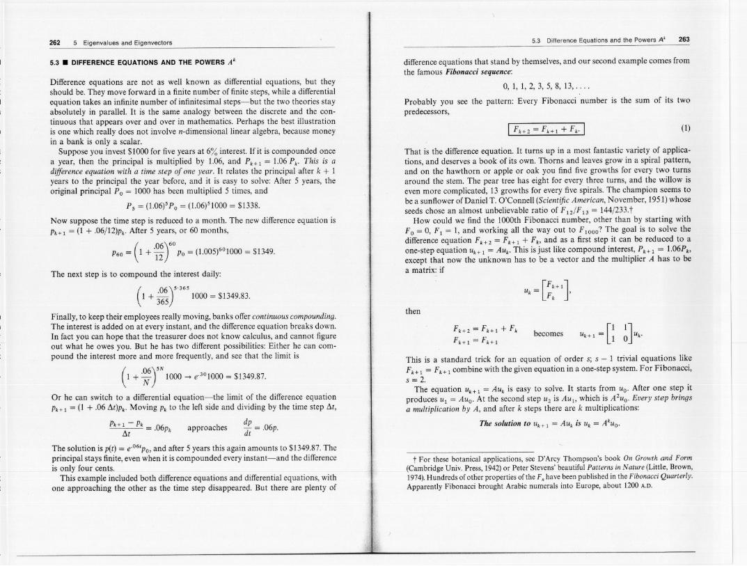
Probably you see the pattern: Every Fibonacci number is the sum of its twopredecessors,

Difference equations are not as well known as differential equations, but theyshould be. They move forward in a finite number of finite steps, while a differentialequation takes an infinite number of infinitesimal steps-but the two theories stayabsolutely in parallel. It is the same analogy between the discrete and the con-tinuous that appears over and over in mathematics. Perhaps the best illustrationis one which really does not involve n-dimensional linear algebra, because moneyin a bank is only a scalar.

Suppose you invest $1000 for five years at 6% interest. If it is compounded oncea year, then the principal is multiplied by 1.06, and PH I = 1.06 Pk. This is adifference equation with a time step of one year. It relates the principal after k + 1years to the principal the year before, and it is easy to solve: After 5 years, theoriginal principal Po = 1000 has been multiplied 5 times, and

P5 = (1.06)5PO= (1.0WI000 = $1338.

Now suppose the time step is reduced to a month. The new difference equation isPH I = (1 + .06/12)Pk'After 5 years, or 60 months,

(06

)60

P60 = 1 + '12 Po = (1.005)601000= $1349.

The next step is to compound the interest daily:

I FH2 = FHI + Fk.1 (1)

That is the difference equation. It turns up in a most fantastic variety of applica-tions, and deserves a book of its own. Thorns and leaves grow in a spiral pattern,and on the hawthorn or apple or oak you find five growths for every two turnsaround the stem. The pear tree has eight for every three turns, and the willow iseven more complicated, 13 growths for every five spirals. The champion seems tobe a sunflower of Daniel T. O'Connell (Scientific American, November, 1951)whoseseeds chose an almost unbelievable ratio of F l2IF 13= l44/233.t

How could we find the 1000th Fibonacci number, other than by starting withF0 = 0, FI = 1, and workingall the way out to F1000?The goal is to solve thedifference equation FH2 = FHI + Fk, and as a first step it can be reduced to aone-step equation UH I = AUk'This is just like compound interest, PH I = 1.06Pk,except that now the unknown has to be a vector and the multiplier A has to bea matrix: if

(.06

)5'365

1 + 365 1000=$1349.83.

- [FHI

J,

Uk - Fk

Finally, to keep their employees really moving, banks offer continuous compounding.

The interest is added on at every instant, and the difference equation breaks down.In fact you can hope that the treasurer does not know calculus, and cannot figureout what he owes you. But he has two different possibilities: Either he can com-pound the interest more and more frequently, and see that the limit is

(1 + ,~YN 1000-+ e.301000= $1349.87.

Or he can switch to a differentialequation-the limit of the differenceequationPH I = (1 + .06 t.t)Pk' Moving Pkto the left side and dividing by the time step t.t,

then

FH2 = FHI + Fk

FHI = FHIbecomes [

1 I

J- Uk'Uk+I - 1 0

PH I - Pk = .06Pk approaches dp = .06p.dt

This is a standard trick for an equation of order s; s - 1 trivial equations like

FH I = FH I combine with the given equation in a one-step system. For Fibonacci,s = 2.

The equation UHI = AUk is easy to solve. It starts from Uo.After one step itproduces UI =Auo. At the second step U2is Aul, which is A2uo. Every step bringsa multiplication by A, and after k steps there are k multiplications:

The solution to UH I = AUk is Uk = Akuo.

The solution is p(t) = e.06,po,and after 5yearsthisagain amountsto $1349.87.Theprincipal stays finite, even when it is compounded every instant-and the differenceis only four cents.

This example included both difference equations and differential equations, withone approaching the other as the time step disappeared. But there are plenty of

t For these botanical applications, see D'Arcy Thompson's book On Growth and Form(Cambridge Univ. Press, 1942) or Peter Stevens' beautiful Patterns in Nature (Little, Brown,1974). Hundreds of other properties ofthe F. have been published in the Fibonacci Quarterly.

Apparently Fibonacci brought Arabic numerals into Europe, about 1200 A.D.


5G'Xf A can

up with fractions and square roots. Somehow these must cancel out, and leave aninteger. In fact, since the second term [(1 - J5)/2]k/J5 is always less than -!,it mustjust move the firs~term to the nearest integer. Slibtraction leaves only the integerpart, and .,

The real problem is to find some quick way to compute the powers Ak, and therebyfind the lOooth Fibonacci number. The key lies in the eigenvalues and eigenvectors:

These formulas give two different approaches to the same solution Uk=SNS-IUO' The first formula recognized that Ak is identical with SAkS-I, and wecould have stopped there. But the second approach brings out more clearly theanalogy with solving a differential equation: Instead of the pure exponential solu-tions e"I'xj, we now have the pure powers A~Xi.The normal modes are again theeigenvectors Xi'and at each step they are amplified by the eigenvalues Ai'By com-bining these special solutions in such a way as to match uo-that is where c camefrom-we recoverthe correct solution Uk= SAkS-IUO'

In any specific example like Fibonacci's, the first step is to find the eigenvalues:

. 1(

1 + J5)1000

F100Q = nearest Integerto J5 --y- .Of course this is an enormous number, and F 1001will be even bigger. It is prettyclear that the fractions are becoming completely insignificant compared to the inte-gers; the ratio F 100dF1000must be very close to the quantity (1 + J5)/2 ~ 1.618,which the Greeks called the "golden mean."t In other words A~is becoming insig-nificant compared. to A1, and the ratio Fu dFk approaches A1+I/A1 = At.

That is a typical example, leading to the powers of A = n AJ.It involved J5because the eigenvalues did. If we choose a different matrix whose eigenvalues arewhole numbers, we can focus on the simplicity of the computation-after the matrixhas been diagonalized:

[-4

A= 10-5

J11 hasAI=l, xl=[_~J. A2=6, X2=[-~J

-IJ[

lk 0

J[2

2 0 6k 1

I

J [2- 6k

1 = - 2 + 2 . 6kAk = SNS-l =[1

-1

A=G ~J. det(A-AI)=A2-A-l,

Al = 1+ J5 '2

= 1 - J52 ,II. 2'

The powers 6kand lk are visible in that last matrix Ak, mixed in by the eigenvectors.For the difference equation Uu I = AUk'we emphasizethe main point. If X is

an eigenvector then

one possible solution is Uo= X,UI= AX,U2= A2X,.. .

When the initial Uohappens to equal an eigenvector, this is the solution: Uk= AkX.

In general Uois not an eigenvector. But if Uois a combination of eigenvectors, thesolution Ukis the same combination of these special solutions.The second row of A - A.Iis (1, - A),so the eigenvector is (A, 1).The first Fibonacci

numbers F0 =0 and F1 = 1go into Uo,andr -- ; ~- __' ." '..", ". . . .

5H If UoFC1Xlf! +CilXn then Uk,=CIA1;>i1-t-. .+ cnX~xn.I c's is to match the.jniti'alcondhiqns:

- --- ..--

Those are the constants in Uk= cIA1xI + C2A~X2.Since the second component ofboth eigenvectors is 1, that leaves Fk = cIA1 + C2A~in the second component ofUk:

rL___

and

Thli.role.of th~Ij,

(4)

_ ...J--We turn to important applications of difference equations-or powers of matrices.

This is the answer we wanted. In one way it is rather surprising, because Fibonacci'srule FU2 = FUI + Fk must always produce whole numbers, and we have ended t The most elegant rectangles have their sides in the ratio of 1.618 to I.


A Markov ProcessThese are the terms CI).~XI+ C2).~X2'The factor ).~= 1 is hidden in the first term,and it is easy to see what happens in the long run: The other factor (.7)kbecomesextremely small, and the solution approaches a limiting state

There was an exercise in Chapter 1,about moving in and out of California, whichis worth another look. These were the rules:

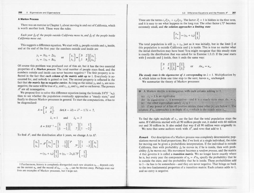
Each year To of the people outside California move in, and -ro of the people insideCalifornia move out.

YI = .9yo + .2zo

ZI = .1yo + .8zoor [YI

J= [

.9 .2

J [yo

J.

Z1 .1.8 Zo

The total population is still Yo + Zo, just as it was initially, but in the limit t 01

this population is outside California and t is inside. This is true no matter whatthe initial distribution may have been! You might recognize that this steady stateis exactly the distribution that was asked for in Exercise 1.3.13. If the year startswith t outside and t inside, then it ends the same way: .

This suggests a difference equation. We start with Yo people outside and Zoinside,and at the end of the first year the numbers outside and inside are

Of course this problem was produced out of thin air, but it has the two essentialproperties of a Markov process: The total number of people stays fixed, and thenumbers outside and inside can never become negative.t The first property is re-flected in the fact that each column of the matrix adds up to 1. Everybody is ac-counted for, and nobody is gained or lost. The second property is reflected in thefact that the matrix has no negative entries. As long as the initial Yo and Zoare non-negative, the same will be true of YI and ZI, Y2and Z2,and so on forever. The powersAk are all nonnegative.

We propose first to solve this difference equation (using the formula SNS-'UO),then to see whether the population eventually approaches a "steady state," andfinally to discuss Markov processes in general. To start the computations, A has tobe diagonalized: .

or

The steady state is the eigenvector of A corresponding to ). = 1. Multiplication byA, which takes us from one time step to the next, leaves u., unchanged.

We summarize the theory of Markov processes:

A =[.9 .2

J.1 .8' det(A - U) = ).2- 1.7).+ .7,

r51 A Markov mithiX is n~n~~a~e. 'wi.th-each 'column addit:ig 1.5J, . 1f

(Ii) ~1'= i'is'an eigenvalue

IP) ii, ,.;~...';\'t"'.:'l '!v,~.."g~"Y~'.d';f ;, a ""'1'1 ,,... ,~"" ,.4~,"'~

(1:;) the,othereigepyalues .s'atisfy~1).il::;;J .' .. qq ;:I.'. .'.

Cd). if'~ny powerpfJA.hils tiiI ;positihe:entries~ th~se. gt~~rJx~f!~~e~beloW'l,;T)1.~oluJ!o~ Ak~g approac\1es ~a_multiple of ;X{"'",;,w~1ChIS the. steady;st~\te.ucq'... -

and To find the right multiple of Xl' use the fact that the total population stays thesame. If California started with all 90 million people out, it ended with 60 millionout and 30 million in. It also ended that way if all 90 million were originally in.

We note that some authors work with AT, and rows that add to 1.

To find At, and the distribution after k years, we change A to N:Remark Our description of a Markov process was completely deterministic; pop-ulations moved in fixed proportions. But if we look at a single individual, the rulesfor moving can be given a probabilistic interpretation. If the individual is outsideCalifornia. then with probability To he moves in; if he is inside. then with prob-ability -rohe moves out. His movement becomes a random process, and the matrixA that governs it is called a transition matrix. We no longer know exactly wherehe is, but every year the components of Uk= AkuO specify the probability that heis outside the state, and the probability that he is inside. These probabilities addto I-he has to be somewhere-and they are never negative. That brings us backto the two fundamental properties of a transition matrix: Each column adds to 1,and no entry is negative.

[Yk

J= Ak [yo

J=

[1 1J [1k kJ [I _1J [

yo

JZk Zo 3 - 3 .7 1 2 Zo

t Furthermore. history is completely disregarded; each new situation Uk+ J depends only

on the current Uk. and the record of Uo. . . . .Uk_ I can be thrown away. Perhaps even ourlives are examples of Markov processes, but I hope not.

268 5 Eigenvalues and Eigenvectors5.3 Difference Equations and the Powers Ak 269

The key step in the theory is to understand why A.= 1 is always an eigenvalue,and why its eigenvector is the steady state. The first point is easy to explain: Eachcolumn of A - I adds up to 1 - 1 = O.Therefore the rows of A - I add up tothe zero row, they are linearly dependent, A - I is singular, and ..1.1= 1 is an eigen-value. Except for very special cases,t Ukwill eventually approach the correspondingeigenvector. This is suggested by the formula Uk= C1A.~X1+ . . . + c"A.~x",in whichno eigenvalue can be larger than 1. (Otherwise the probabilities Ukwould blow uplike Fibonacci numbers.) If all other eigenvalues are strictly smaller than ..1.1= 1,then the first term in the formula will be completely dominant; the other A.~go tozero, and Uk-->C1X1= UCO'

This is an example of one of the central themes of this chapter: Given informa-tion about A, find information about its eigenvalues. Here we found A..nax= 1.

There is an obvious difference between Fibonacci numbers and Markov

processes. The numbers Fk become larger and larger, while by definition any"probability" is between 0 and 1. The Fibonacci equation is unstable, and so isthe compound interest equation PH 1 = 1.06Pk; the principal keeps growing for-ever. If the Markov probabilities decreased to zero, that equation would be stable;but they do not, since at every stage they must add to 1. Therefore a Markovprocess is neutrally stable.

Now suppose we are given any difference equation UH 1 = AUk' and we wantto study its behavior as k -->00. Assuming A can be diagonalized, the solution Ukwill be a combination of pure solutions, .

is certainly stable; its eigenvalues are 0 and t, lying on the main diagonal becauseA is triangular.Starting fromanyinitial vector uo, and following the rule Uk+1 =AUk'the solution must eventuallyapproach zero:

You can see how the larger eigenvalue A.= i governs the decay; after the first stepevery vector Ukis half of the preceding one. The real effect of the first step is tosplit Uo into the two eigenvectors of A,

and to annihilate the second eigenvector (corresponding to A.=0). The first eigen-vector is multiplied by A.= t at every step.

Positive Matrices and Applications

By developing the Markov ideas we can find a small gold mine (entirely optional)of matrix applications in economics.

EXAMPLE1 Leontief's input-output matrixThis is one of the first great successes of mathematical economics. To illustrate it,we construct a consumptionmatrix-in which au gives the amount. of product jthat is needed to create one unit of product i:

The growth of Uk is governed by the factors A.~,and stability depends on theeigenvalues.

5J The diffetenceequation Uk+ 1=; AUk.'isI . .

!stable ifall eigenvalu!"ssatisfy 1::1:11<f If

I

neutrally.;stableifSbme J.A.jr~ 'land.t}1e ot4~fil~} <duns,tableIf at least one eigenvalue haslhL>'l,

I~ t~e~able ~e~ ~hepowersAkapp~ac_h..::r~ :nd so~~~~.:!oluiiOn

[

.4 0 .1

]A = 0 .1 .8

.5 .7 .1

(steel)(food)(labor)

A = [~ :J

Thefirst question is: Can we produce Yl units of steel,Y2 units of food,and Y3units of labor? To do so, we must start with larger amounts PI' P2, P3' becausesome part is consumed by the production itself. The amount consumed is Ap, andit leaves a net production of p - Ap.

Problem To find a vector p such that p - Ap = y, or p = (I - A) -I y.

On the surface, we are only asking if I - A is invertible. But there is a nonnegative

twist to the problem.Demand and production,y and p, are nonnegative.Sincepis (I - A) -I y, the real question is about the matrix that multiplies y:

When is (I - A) -1 a nonnegative matrix?

EXAMPLE The matrix

t If everybody outside moves in and everybody inside moves out, then the populationsare reversedevery year and there is no steady state. The transition matrix is A = [? AJand -1 is an eigenvalueas wellas + I-which cannot happen if all aij> O.


I(I - A)-' = 1 + A + A2 + A3+ I (5)

for the next set of values A2pO' The question is whether the prices approach equi-librium. Are there prices such that p = Ap, and does the system take us there?

You recognize p as the (nonnegative) eigenvector of the Markov matrix A-corresponding to A = 1. It is the steady state Pro, and it is approached from anystarting point Po. The economy depends on this, that by repeating a transactionover and over the price tends to equilibrium.

For completeness we give a quick explanation of the key properties of a posi-tivematrix-not to be confused with a positive definite matrix, which is symmetricand has all its eigenvalues positive. Here all the entries aij are positive.

Roughly speaking, A cannot be too large. If production consumes too much,nothing is left as output. The key is in the largest eigenvalue A, of A, which mustbe below 1:

If A, > 1,(I - A)-, fails to be nonnegative

If A, = 1,(1 - A)-' fails to exist

If A, < 1,(I - A)-' is a sumof nonnegative matrices:

The 3 by 3 example has A, = .9 and output exceedsinput. Productioncan go on.Thoseareeasyto prove,once we know the main fact about a nonnegativema-

trix like A: Not only is the largest eigenvalue positive, but so is the eigenvectorx ,. Then (I - A) -, has the same eigenvector, with eigenvalue 1/(1 - A,).

If A, exceeds 1, that last number is negative. The matrix (I - A) -, will take thepositive vector x, to a negative vector xtl(1 - A,). In that case (I - A)-' is defi-nitely not nonnegative. If A, = 1, then 1 - A is singular. The productive case ofa healthy economyis A, < 1,when the powersof A go to zero (stability) and theinfiniteseries1 + A + A2 + . . . converges.Multiplyingthis seriesby 1 - A leavesthe identity matrix-all higher powers cancel-so (I - A)-' is a sum of non-negative matrices. We give two examples:

fSk- the-la~ge$teig;rl\';llie A, ofa p()sitiv; m~ilixis r;;1 alld positive, a.nds4arethe componentsof theeigenvectorXI. I---

A = [~

A =[~ .~J has A, = ~ and we can produce anything.

Proof Suppose A > O.The key idea is to look at all numbers t such that Ax ~ txfor some nonnegative vector x (other than x = 0). We are allowing inequality inAx ~ tx in order to have many positive candidates t. For the largest value tm.,

(which is attained), we will show that equality holds: Ax = tmaxx.Otherwise, if Ax ~ tmaxx is not an equality, multiply by A. Because A is positive

that produces a strict inequality A2x > tmaxAx.Therefore the positive vector y = Axsatisfies Ay > tmaxY, and tmax could be increased. This contradiction forces theequality Ax = tmaxx,and we have an eigenvalue. Its eigenvector x is positive be-cause on the left side of that equality Ax is sure to be positive.

To see that no eigenvaluecan be larger than tmax, supposeAz = AZ.SinceAandz may involve negative or complex numbers, we take absolute values: IAlizl=IAzl::::;Aiziby the"triangle inequality."This Iziis a nonnegativevector, so IAI isone of the possible candidates t. ThereforeIAI cannot exceed tmax-which must bethe largest eigenvalue.

~J has A, = 2 and the economy is lost

The matrices (I - A)-' in thosetwocasesare[:1 :n arid[~ nLeontief's inspiration was to find a model which uses genuine data from the

real economy; the U.S. table for 1958 contained 83 industries, each of whom sent

in a complete "transactions table" of consumption and production. The theoryalso reaches beyond (I - A)-', to decide natural prices and questionsof opti-mization. Normally labor is in limited supplyand ought to be minimized.And,of course,the economy is not always linear.

This is the Perron-Frobenius theorem for positive matrices, and it has one moreapplication in mathematical economics.

EXAMPLE3 Von Neumann's model of an expanding economyWe go back to the 3 by 3 matrix A that gave the consumptionofsteel,food,andlabor. If the outputs are 5" Ip I" then the required inputs are

EXAMPLE2 The prices in a closed input-output modelThe model is called "closed" when everything produced is also consumed. Nothinggoes outside the system. In that case the matrix A goes back to a Markov matrix.The columns add up to 1. We might be talking about the value of steel and foodand labor, instead of the number of units. The vector p represents prices insteadof production levels.

Suppose Po is a vector of prices. Then Apo multiplies prices by amounts togive the value of each product. That is a new set of prices, which the system uses

[

.4 0 .1

] [

5,

]uo= 0 .1 .8 I, = Au,.

.5 .7.1 I,

In economics the difference equation is backward! Instead of u, = Auo we have

uo = Au,. If A is small (as it is), then production does not consume every thing-and the economy can grow. The eigenvalues of A -, will govern this growth. Butagain there is a nonnegative twist, since steel, food, and labor cannot come in

272 5 Eigenvalues and.Eigenvectors 5.3 Difference Equations and the Powers A. 273

negativeamounts. Yon Neumann asked for the maximum rate t at which theeconomy can expand and still stay nonnegative, meaning that ul ~ tuo ~ 0.

Thus the problem requires UI ~ tAuI' It is like the Perron-Frobenius theorem,with A on the other side. As before, equality holds when t reaches tmax-which isthe eigenvalue associated with the positive eigenvector of A -I. In this examplethe expansion factor is if:

5.3.6 Write down the 3 by 3 transition matrix for a chemistry course that is taught intwo sections, if every week i of those in Section A and! of those in SectionB dropthe course, and! of each section transfer to the other section.

Find the limitingvaluesof Y. and z. (k 00)if5.3.7

YH 1 = .8y. + .3z.ZH I = .2y. + .7z.

Yo= 0Zo= 5.

X~m

and

[

.4 ° .1

] [

1

] [

0.9

]

9Ax = ° .1 .8 5 = 4.5 = 10x.

.5 .7 .1 5 4.5 5.3.8

Also find formulas for Y. and z. from A. = sNS- I.

(a) From the fact that column 1 + column 2 = 2 (columIl 3), so the columns arelinearly dependent, what is one of the eigenvalues of A and what is its corresponding

eigenvector? 'With steel-food-Iabor in the ratio 1-5-5, the economy grows as quickly as possible:The maximum growth rate is 1/,,1,1'

EXERCISES [

.2A = .4

.4

.4 .3

].2 .3 ..4 .4

5.3.1 (a) For the Fibonacci matrix A = n n write down A2, A3, A4, and then (usingthe text) A 100.

(b) Find B-101 if B = [-1 ~n

5.3.2 Suppose Fibonacci had started his sequence with F0 = 1 and FI = 3, and thenfollowedthe same rule FH2 =FHI + F.. FindthenewinitialvectorUo,thenewcoefficientsc = S-IUO,and the new Fibonacci numbers. Show that the ratiosFH 1IF. still approach the golden mean.

5.3.3 If each number is the average of the two previous numbers, GH2 = t(GHI + G.),set up the matrix A and diagonalize it. Starting from Go = 0 and GI = t, find aformula for G. and compute its limit as k 00.

5.3.4 BernadeJli studied a beetle "which lives three years only, and propagates in its thirdyear." If the first age group survives with probability t, and then the secondwithprobability!, and then the third produces six females on the way out, the matrix is

(b) Find the other eigenvalues of A.(c) If Uo= (0, 10,0) find the limit of A.uo as k 00.

5.3.9 Suppose there are three major centers for Move-It-Yourself trucks. Every monthhalf of those in Boston and in Los Angeles go to Chicago, the other half stay wherethey are, and the trucks in Chicago are split equa!ly between Boston and LosAngeles. Set up the 3' by 3 transition matrix A, and find the steady state u'" cor-respondingto the eigenvalueA. = 1.

5.3.10 (a) In what range of a and b is the followingequation a Markov process?)

uH 1 = Au. = [1 ~ a 1:b]u., Uo= G 1

[

0 0 6

]A= tOO.

o ! 0

(b) Compute u. = SNS-IUO for any a and b.(c) Under what condition on a and b does u. approach a finite limit as k 00,and what is the limit? Does A have to be a Markov matrix?

5.3.11 Multinational companies in the U.S., Japan, and Europe have assets of $4 trillion.At the start, $2 trillion are in the U.S. and $2 trillion in Europe. Each year t theU.S. money stays home, i goes to both Japan and Europe. For Japan and Europe,

t stays home and t is sent to the U.S.(a) Find the matrix that givesShow that A3 = I, and follow the distribution of beetles for six years starting with

3000 beetles in each age group.

5.3.5 Suppose there is an epidemic in which every month half of those who are wellbecome sick, and a quarter of those who are sick become dead. Find the steady statefor the corresponding Markov process [n..., ~A[n."

[

dH I

] [

1 i 0

] [

d.

]

SH 1 = 0 its. .WHI 0 0 t w.

(b) Find the eigenvalues and eigenvectors of A.(c) Find the limiting distribution of the $4 trillion as the world ends.

(d) Find the distribution a~year k.


5.3.12 If A is a Markov matrix, show that the sum of the components of Ax equals thesum of the components of x. Deduce that if Ax = Ax with A #- 1, the componentsof the eigenvector add to zero.

5.3.13 The solution to dujdt = Au = [~ -~]u (eigenvalues i and - i) goes around in acircle: u = (cos t, sin t). Suppose we approximate by forward, backward, and centereddifference equations:(a) U.+1 - u. = Au. or U.+1= (I + A)u.(b) U.+1 - u. = AU.+I or U.+I = (I - A)-IU.(c) u.+ I - u. = tA(u.+ I + u.) or u.+ I = (I - tA)-I(I + tA)u..Find the eigenvalues of 1 + A and (1 - A)-I and (I - tA)-I(I + tA). For whichdifference equation does the solution stay on a circle?

5.3.14 For the system v.+I = IX(V.+ w.), W.+I = IX(V.+ w.), what values of IX produceinstability?

5.3.15 Find the largest valuesa, b, c for which these matrices are stable or neutrally stable:

[a -.8

J.8 .2' [b .8

J° .2 ' [c .8

J.

.2 c

5.3.16 Multiplying term by term, check that (1 - A)(1 + A + A 2 + . . .) = 1. This infiniteseries represents (I - A) - I, and is nonnegative whenever A is nonnegative'; providedit has a finite sum; the condition for that is AI < I. Add up the infinite series,andconfirm that it equals (I - A) -1, for the consumption matrix

[

0 1 1

]A= ° ° 1 .

° ° °

5.3.17 For A = [g n find the powers Ak (including AO) and show explicitly that theirsum agrees with (1 - A)- I.

5.3.18 Explain by mathematics or economicswhy increasing any entry of the "consump-tion matrix" A must increase tmax= AI (and slow down the expansion).

5.3.19 What are the, limits as k -+ 00 (the steady states) of

[.4 .2

J

k

[I

J.6.8 ° [.4 .2

J

k

[O

J.6.8 1 [.4 .2

Jk?

.6 .8and and

5.3.20 Prove that every third Fibonacci number is even.

5.4 Differential Equations and the Exponential e'" 275

DIFFERENTIALEQUATIONSAND THE EXPONENTIAL eAI . 5.4

il'-:~,

Wherever you find a system of equations, rather than a single equation, matrixtheory has a part to play.This was true for differenceequations, wherethe solutionUk= Akuodepended on the powersof A. It is equally true for differentialequations,where the solution u(t)= eA1uodepends on the exponential of A. To define thisexponential, and to understand it, we turn right away to an example:

~~ = Au =[- ~ -~}.(1)

The first step is always to find the eigenvalues and eigenvectors:

A[~J = (-l)GJ. A[ -~J = (-3{ _~}'I~

Then there are several possibilities,all leading to the same answer. Probably thebest way is to write down the general solution, and match it to the initia.1vectorUoat t = O.Thegeneralsolutionis a combinationofpure exponentialsolutions.Theseare solutionsofthe specialformceA1x,where A.is an eigenvalueof A and xis its eigenvector;they satisfy the differentialequation, sinced/dt(ceAlx)= A(ceA1x).(They were our introduction to eigenvalues,at the start of the chapter.) In this 2by 2 example, there are two pure exponentials to be combined:

~!~

[1 I

J [e-'

J [CI

Ju= 1 -1 e-31 c2'

At timezero,whenthe exponentialsare eO= 1,Uodetermines Cl and C2:

(2)u(t) = cleAtlxl + c2eA21x2 or

Uo = CIXI + C2X2uo=G _~J[~J=sc.

or~i,Ii

You recognizeS, the matrix of eigenvectors.And the constants c = S-lUO are thesame as they were for differenceequations. Substituting them back into (2), theproblem is solved. In matrix form, the solution is

u(t)= G -~J [e-' e-31J[~J = s[e-' e-3IJS-IUO'

Here is the fundamental formula of this section: u = SeAIS-luo solves the differen-tial equation, just as sNs -lUO solved the difference equation. The key matrices are

A=[ -1 -3Jand

eAI= [e-' e-31}

linear algebra and its applica tions - penn …kazdan/260s12/notes/vectors/strang... · linear...

Documents