Limits and Their Properties1

Copyright © Cengage Learning. All rights reserved.

2

Day 2

BC Limits Review

Limits involving Infinity

Handout: (Introduction to Limits (Graphical)WS)

Copyright © Cengage Learning. All rights reserved.

1.4B-1.5& 3.5

3

One-Sided Limits and Continuity on a Closed Interval

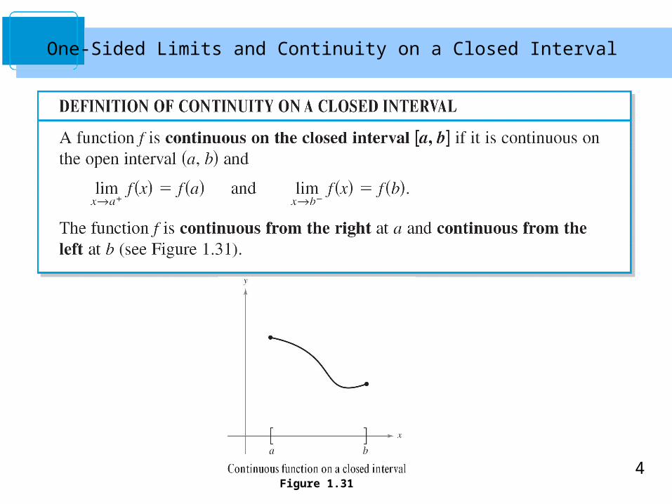
4Figure 1.31

One-Sided Limits and Continuity on a Closed Interval

5

Example 4 – Continuity on a Closed Interval

Discuss the continuity of f(x) =

Solution:The domain of f is the closed interval [–1, 1].

6

Example 4 – Solution

Figure 1.32

cont’d

Because

and

you can conclude that f is continuous on the closed interval [–1, 1], as shown in Figure 1.32.

7

Most of the techniques of calculus require that functions be continuous. A function is continuous if you can draw it in one motion without picking up your pencil.

A function is continuous at a point if the limit is the same as the value of the function.

This function has discontinuities at x=1 and x=2.

It is continuous at x=0 and x=4, because the one-sided limits match the value of the function1 2 3 4

1

2

8

Properties of Continuity

9

Properties of Continuity

Continuous functions can be added, subtracted, multiplied, divided and multiplied by a constant, and the new function remains continuous.

10

Example – Applying Properties of Continuity

By Theorem 1.11, it follows that each of the functions below is continuous at every point in its domain.

11

The Intermediate Value Theorem(IVT)

12

The Intermediate Value Theorem

In other words

13

Intermediate Value Theorem

If a function is continuous between a and b, then it takes on every value

between and . f a f b

a b

f a

f b Because the function is continuous, it must take on every y value between and .

f a f b

15

Suppose that a girl is 5 feet tall on her thirteenth birthday and

5 feet 7 inches tall on her fourteenth birthday.

Then, for any height h between 5 feet and 5 feet 7 inches,

there must have been a time t when her height was exactly h.

This seems reasonable because human growth is continuous

and a person’s height does not abruptly change from one

value to another.

The Intermediate Value Theorem

16

The Intermediate Value Theorem guarantees the existence of at least one number c in the closed interval [a, b] .

There may, of course, be more than one number c such that f(c) = k, as shown in Figure 1.35.

Figure 1.35

The Intermediate Value Theorem

17

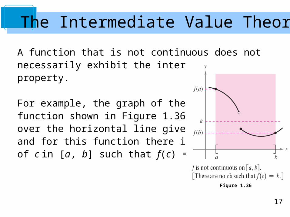
A function that is not continuous does not necessarily exhibit the intermediate value property.

For example, the graph of the function shown in Figure 1.36 jumps over the horizontal line given by y = k, and for this function there is no value of c in [a, b] such that f(c) = k.

Figure 1.36

The Intermediate Value Theorem

19

Example – An Application of the Intermediate Value Theorem

Use the Intermediate Value Theorem to show that the polynomial function has a zero in the interval [0, 1].

Solution:

Note that f is continuous on the closed interval [0, 1].

Because

it follows that f(x) must pass through zero in the interval [0,2].

3 2 1f x x x

1f 0f

20

Solution

You can therefore apply the Intermediate Value Theorem to conclude that there must be some c in [0, 1] such that

as shown in Figure 1.37.

Figure 1.37

cont’d

21

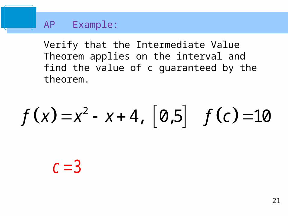
AP Example:

Verify that the Intermediate Value Theorem applies on the interval and find the value of c guaranteed by the theorem.

2 4, 0,5 10f x x x f c

3c

22

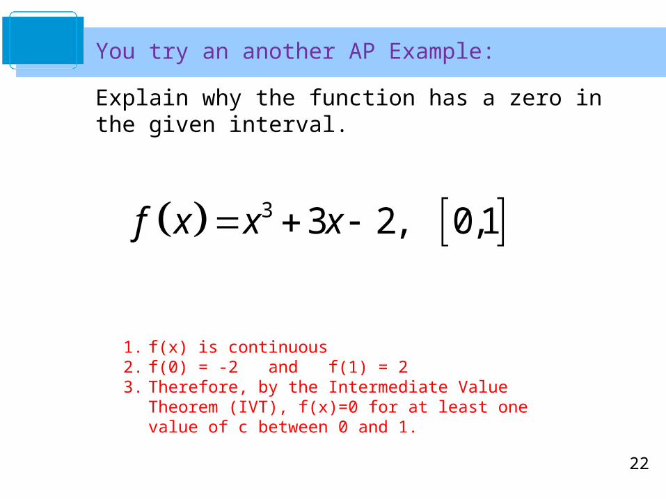
You try an another AP Example:

Explain why the function has a zero in the given interval.

3 3 2, 0,1f x x x

1. f(x) is continuous2. f(0) = -2 and f(1) = 23. Therefore, by the Intermediate Value Theorem (IVT),

f(x)=0 for at least one value of c between 0 and 1.

23

Discuss with your neighbor

• Name the three conditions that must be met for a function to be continuous at a point.

lim existsx cf x

limx cf x f c

is definedf c

24

Infinite Limits1.5

25

Infinite Limits:

1f x

x

0

1limx x

As the denominator approaches zero, the value of the fraction gets very large.

If the denominator is positive then the fraction is positive.

0

1limx x

If the denominator is negative then the fraction is negative.

vertical asymptote at x=0.

0

1lim ?x x

26

Limits at infinity:

1f x

x

What happens to the value of this expression as the denominator approaches either positive or negative infinity?

vertical asymptote at x=0.

0xx

1lim

xx

1lim

0

27

Example – Determining Infinite Limits from a Graph

Determine the limit of each function shown in Figure 1.41 as x approaches 1 from the left and from the right.

Figure 1.41

31

Example 2 – Finding Vertical Asymptotes

Determine all vertical asymptotes of the graph of each function.

32

Example 2(a) – Solution

When x = –1, the denominator of is 0 and the numerator is not 0.

So, by Theorem 1.14, you can conclude that x = –1 is a vertical asymptote, as shown in Figure 1.42(a).

Figure 1.42(a).

33

By factoring the denominator as

you can see that the denominator is 0 at x = –1 and x = 1.

Moreover, because the numerator is not 0 at these two points, you can apply Theorem 1.14 to conclude that the graph of f has two vertical asymptotes, as shown in figure 1.42(b).

cont’dExample 2(b) – Solution

Figure 1.42(b)

34

By writing the cotangent function in the form

you can apply Theorem 1.14 to conclude that vertical asymptotes occur at all values of x such thatsin x = 0 and cos x ≠ 0, as shown in Figure 1.42(c).

So, the graph of this function has infinitely many vertical asymptotes. These asymptotes occur at x = nπ, where n is an integer.

cont’d

Figure 1.42(c).

Example 2(c) – Solution

35

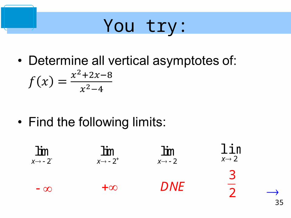
You try:

2limx 2

limx 2

limx

DNE

2limx

3

2

36

37

You try:• Find the limit:

a)

b)

c)

x

xx

1

2lim

1

xx

x

1lim 2

0

xxx

tanlim 2

2/1

DNE

3939

This section discusses the “end behavior” of a function

on an infinite interval. Consider the graph of

as shown in Figure 3.33.

Limits at Infinity

Figure 3.33

4040

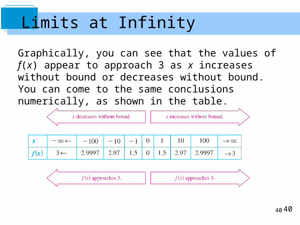
Graphically, you can see that the values of f(x) appear to approach 3 as x increases without bound or decreases without bound. You can come to the same conclusions numerically, as shown in the table.

Limits at Infinity

4141

The table suggests that the value of f(x) approaches 3 as x increases without bound . Similarly, f(x) approaches 3 as x decreases without bound .

These limits at infinity are denoted by

and

Limits at Infinity

4242

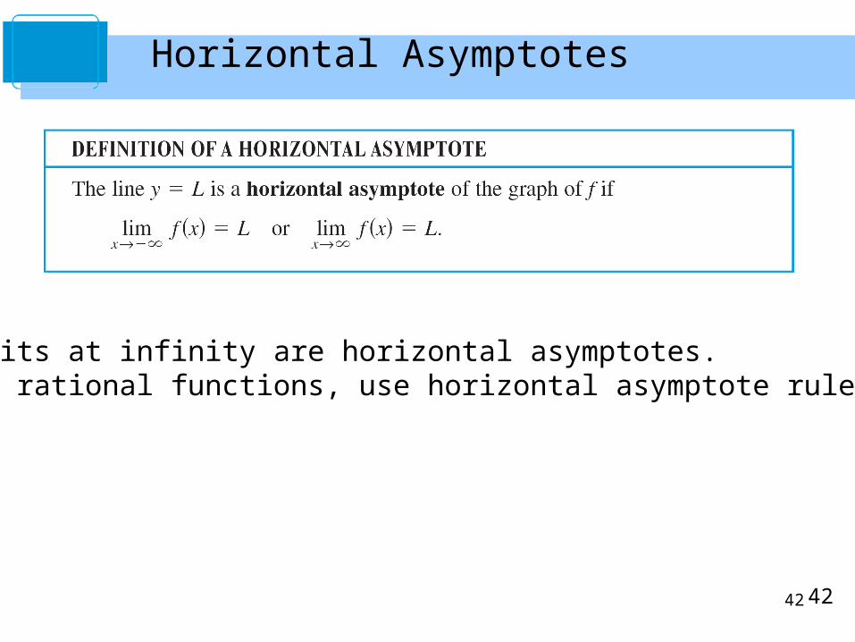
Limits at infinity are horizontal asymptotes.For rational functions, use horizontal asymptote rules.

Horizontal Asymptotes

43

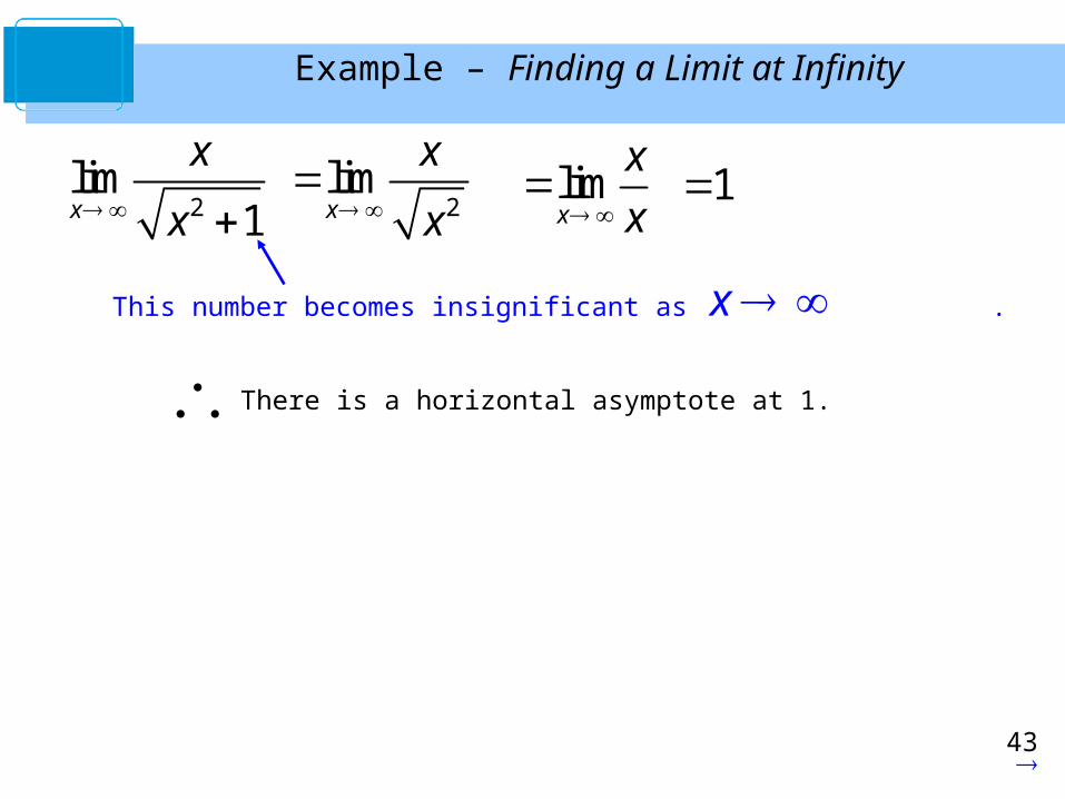
2lim

1x

x

x 2limx

x

x

This number becomes insignificant as .x

limx

x

x 1

There is a horizontal asymptote at 1.

Example – Finding a Limit at Infinity

45

sin xf x

x

Example:

sinlimx

x

x Find:

When we graph this function, the limit appears to be zero.

1 sin 1x

so for :0x 1 sin 1x

x x x

1 sin 1lim lim limx x x

x

x x x

sin0 lim 0

x

x

x

by the sandwich theorem:

sinlim 0x

x

x

46

Example: 5 sinlimx

x x

x

Find:

5 sinlimx

x x

x x

sinlim 5 limx x

x

x

5 0

5

4747

Example – Finding a Limit at Infinity

Find the limit:

Solution: Using Theorem 3.10, you can write

4848

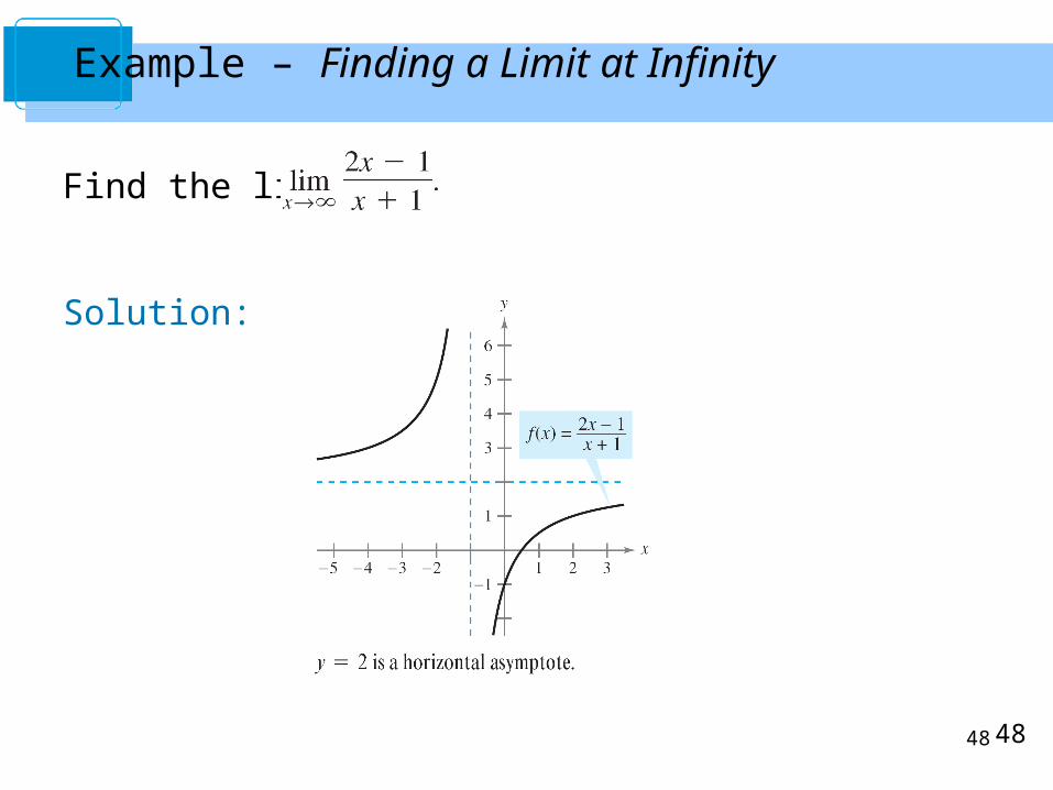
Example – Finding a Limit at Infinity

Find the limit:

Solution:

49

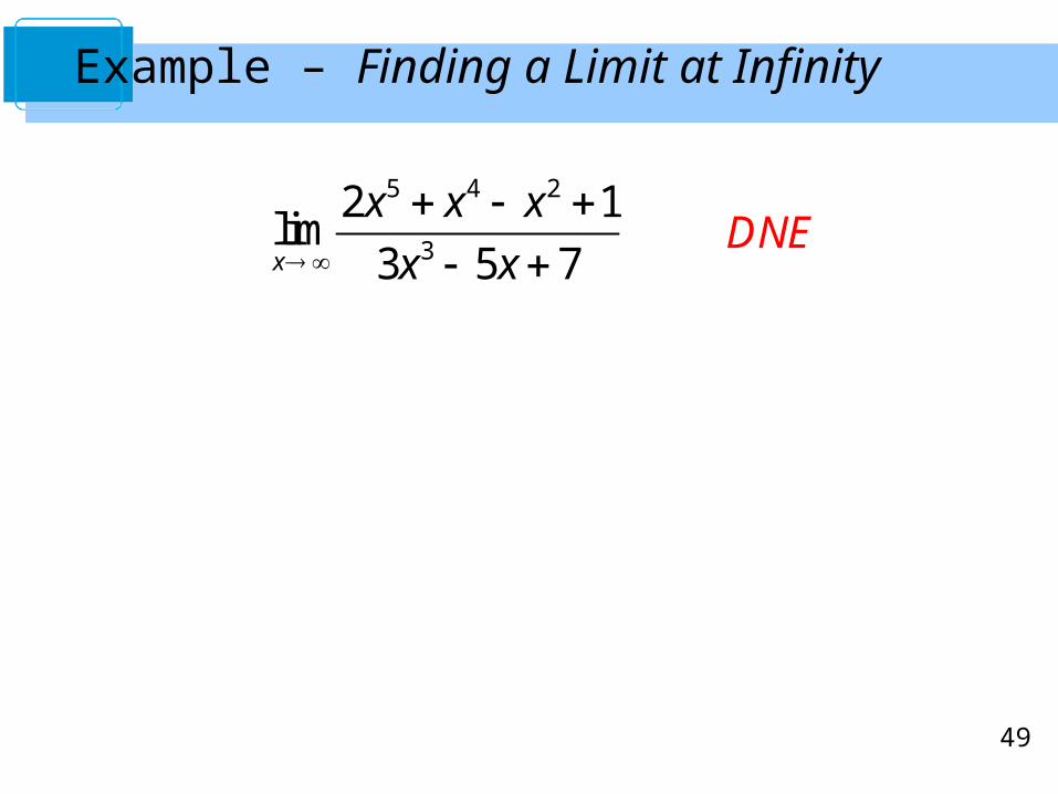
5 4 2

3

2 1lim

3 5 7x

x x x

x x

DNE

Example – Finding a Limit at Infinity

50

02

3

2 1lim

3 5 7x

x x

x x

Example – Finding a Limit at Infinity

5151

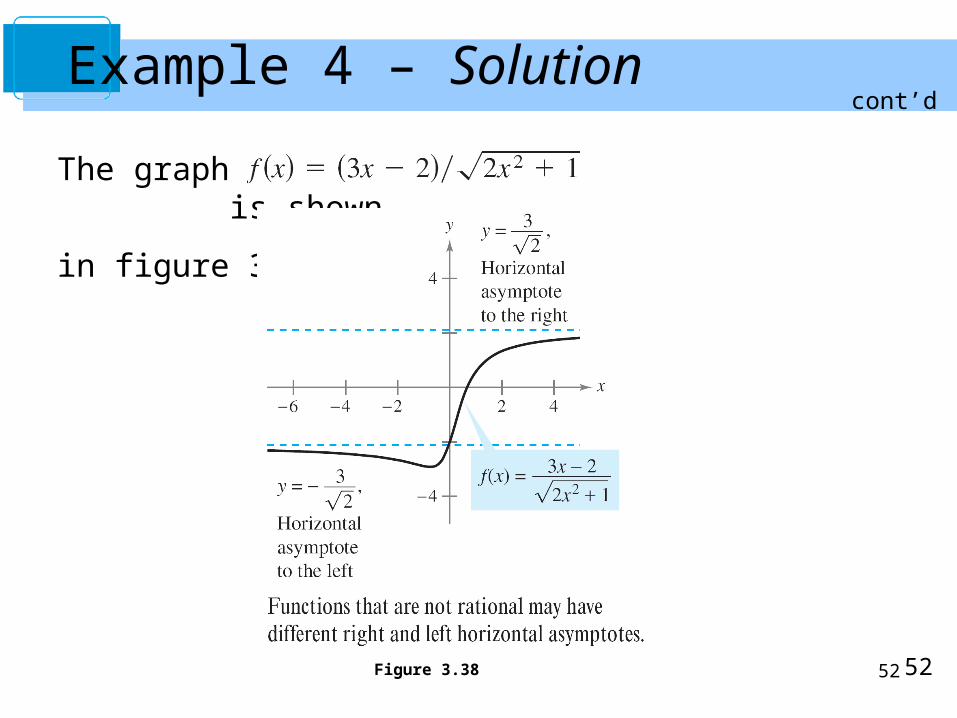
Example – A Function with Two Horizontal Asymptotes

Find each limit.

5252

The graph of is shown

in figure 3.38.

Example 4 – Solution

Figure 3.38

cont’d

53

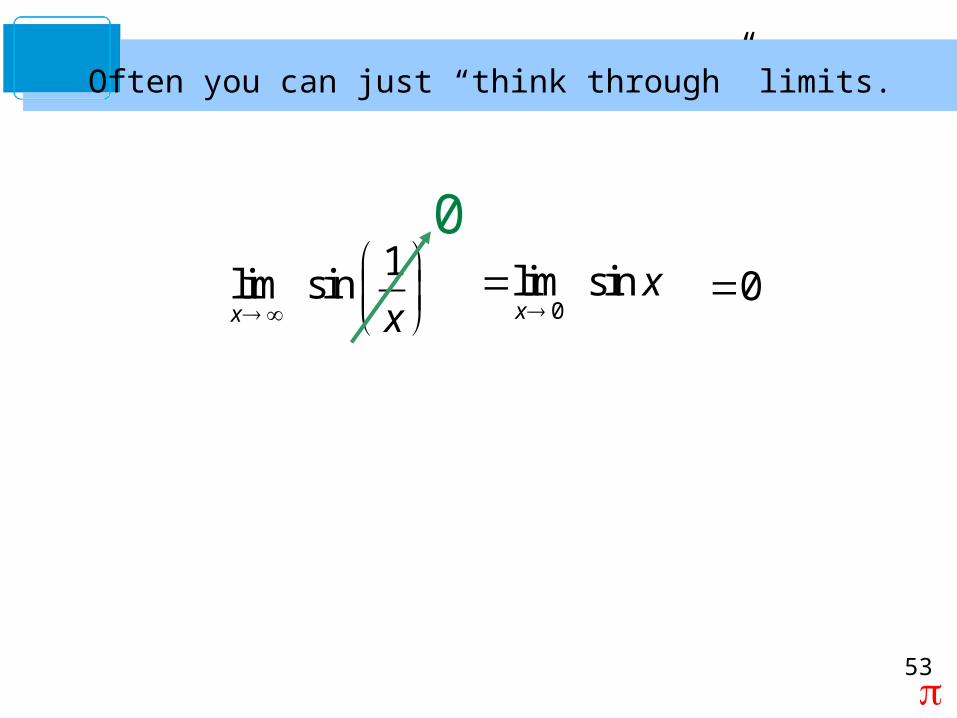
Often you can just “think through” limits.

1lim sinx x

0

0lim sinx

x

0

5454

Find each limit.

Solution:

a. As x increases without bound, x3 also increases without bound. So, you can write

b. As x decreases without bound, x3 also decreases without bound. So, you can write

Example – Finding Infinite Limits at Infinity

5555

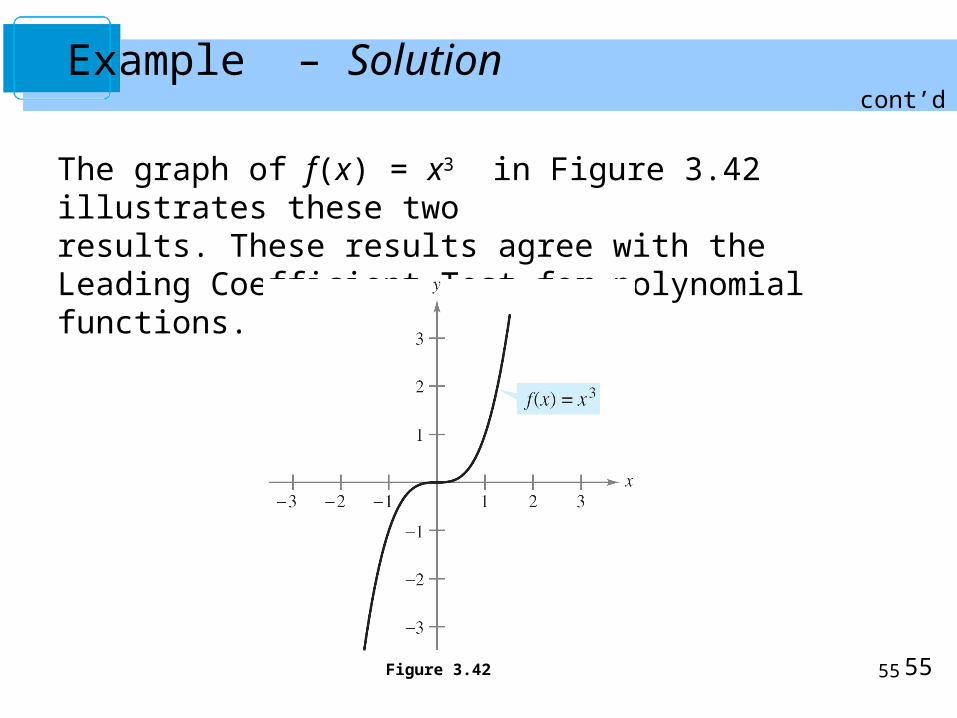
Example – Solution

The graph of f(x) = x3 in Figure 3.42 illustrates these two results. These results agree with the Leading Coefficient Test for polynomial functions.

Figure 3.42

cont’d

56

Discuss with your group

5.at x asymptote horizontal

a and 2,at x asymptote verticala -3,at x hole a

0,at x zero aith function w a ofequation theWrite

57

Theorem 1.1

You are in Calculus, therefore you rock!

58

HWQ

Find the following limit:

58

1

2lim

1x

x

x

59

Homework

• MMM pgs. 30-31

• + 76,77,83,84 pg. 80 Larson

59

60

HWQ

Find the following limit:

60

1lim cosx x

1

61

HWQ

Find the following limit:

61

1

2lim

1x

x

x