limitations of a linear model for the hurricane ... - lmu

QUARTERLY JOURNAL OF THE ROYAL METEOROLOGICAL SOCIETYQ. J. R. Meteorol. Soc. 135: 839–850 (2009)Published online 15 April 2009 in Wiley InterScience(www.interscience.wiley.com) DOI: 10.1002/qj.390

Limitations of a linear model for the hurricane boundarylayer

Stefanie Vogl and Roger K. Smith*Meteorological Institute, University of Munich, Germany

ABSTRACT: The linear model for the steady boundary layer of a rapidly rotating axisymmetric vortex is derived from adetailed scale analysis of the full equations of motion. The previously known analytic solution is re-appraised for vorticesof hurricane scale and strength. The internal consistency of the linear approximation is investigated for such a vortexby calculating from the solution the magnitude of the nonlinear terms that are neglected in the approximation comparedwith the terms retained. It is shown that the nonlinear terms are not negligibly small in a large region of the vortex, afeature that is consistent with the scale analysis. We argue that the boundary-layer problem is well-posed only at outerradii where there is subsidence into the layer. At inner radii, where there is ascent, only the radial pressure gradient may beprescribed and not the wind components at the top of the boundary layer, but the linear problem cannot be solved in thesecircumstances. We examine the radius at which the vertical flow at the top of the boundary layer changes sign for differenttangential wind profiles relevant to hurricanes and show that this is several hundred kilometres from the vortex centre.This feature represents a further limitation of the linear model applied to hurricanes. While the present analysis assumesaxial symmetry, the same limitations presumably apply to non-axisymmetric extensions to the linear model. Copyright c©2009 Royal Meteorological Society

KEY WORDS hurricanes; tropical cyclones; typhoons; boundary layer; friction layer

Received 21 October 2008; Revised 14 January 2009; Accepted 22 January 2009

1. Introduction

The boundary layer of a mature hurricane is an importantfeature of the storm, as it strongly constrains the radialdistribution of vertical motion at its top, as well as the dis-tributions of absolute angular momentum and moisture. Infact, there is mounting evidence that the boundary layerplays a central role in the hurricane intensification pro-cess itself (e.g. Emanuel, 1997; Smith et al., 2008, 2009).Over the years the boundary layer has been the subject ofnumerous theoretical investigations, many of them relat-ing to axisymmetric vortices (Rosenthal, 1962; Miller,1965; Smith, 1968; Leslie and Smith, 1970; Carrier,1971; Eliassen, 1971; Bode and Smith, 1975; Eliassenand Lystadt, 1977; Montgomery et al., 2001; Smith, 2003;Smith and Montgomery, 2008; Smith and Vogl, 2008) anda few also to asymmetric vortices (Shapiro, 1983; Kepert,2001; Kepert and Wang, 2001). These studies can bedivided into three types: vertically integrated models thatassume certain profiles of the radial and tangential windcomponents, but not their scales (Smith, 1968; Leslieand Smith, 1970; Bode and Smith, 1975); slab models,which are a subset of the former that assume uniformprofiles (Shapiro, 1983; Smith, 2003; Smith and Vogl,2008; Smith and Montgomery, 2008); and what we willterm ‘continuous models’, in which the vertical structure

∗Correspondence to: Roger K. Smith, Meteorological Institute, Univer-sity of Munich, Theresienstr. 37, 80333 Munich, Germany.E-mail: [email protected]

is determined as well as the radial structure (Eliassen,1971; Eliassen and Lystadt, 1977; Montgomery et al.,2001; Kepert, 2001; Kepert and Wang, 2001). With theexception of Smith (2003) and Smith and Vogl (2008),all of the aforementioned studies have focused on thedynamical aspects of the boundary layer: thermodynamicaspects were not considered.

In one of the early studies, Eliassen (1971) developeda linear theory for the spin-down of a vortex as aresult of surface friction and showed that, if a no-slipcondition is applied at the surface, the temporal decayof the tangential winds above the boundary layer isexponential. He showed also that the vertical velocityat the top of the boundary layer is upwards and nearlyconstant inside the radius of maximum tangential winds,with a maximum at the vortex centre. However, in thecase of a turbulent boundary layer, the vortex decaysalgebraically with time. Moreover, the vertical velocityat the top of the boundary layer is zero at the vortexcentre and increases linearly with radius inside the radiusof maximum tangential winds.

Eliassen and Lystadt (1977) extended this work toaccount for differential rotation in the tangential flow andpresented numerical solutions of the coupled equationsfor the boundary layer and the vortex above for the casewith a quadratic drag law in the surface layer. Their spin-down theory predicts the evolution of the angular veloc-ity, the transverse streamfunction and the boundary-layerdepth, as well as the half-life time of the vortex (the time

Copyright c© 2009 Royal Meteorological Society

840 S. VOGL AND R. K. SMITH

required to reduce the angular velocity by one half). Thetheory is formulated in an inertial (non-rotating) coor-dinate system and assumes that the flow evolves closeto a state of cyclostrophic balance throughout the fluid.However, the strongest vortex examined had a maximumspeed of only 10 m s−1, corresponding to a Rossby num-ber of 20 at the latitude considered. Montgomery et al.(2001) pointed out that the neglected non-cyclostrophicterms in the boundary layer may become significant athigher swirl speeds, which might limit the applicabil-ity of the theory to hurricanes. To investigate this issuethey performed numerical calculations of the full nonlin-ear equations in the same spin-down flow configurationas Eliassen and Lystadt, and obtained solutions for vor-tices of different intensities including hurricane-strengthvortices (i.e. with maximum tangential winds exceeding33 m s−1). They found that the theoretically predictedalgebraic temporal decay of the primary vortex is vali-dated also for tropical storm and hurricane-strength vor-tices, but noted increasing quantitative departures fromEliassen and Lystadt’s theory with increasing fluid depth,although it is still qualitatively valid for hurricane-likevortices 10 and 15 km deep. They found also that, asthe vortex strength increases from tropical storm to hur-ricane strength, the cyclostrophic balance approximationbecomes only marginally valid in the boundary layer yetremains valid in the flow interior. In addition, a tempo-rary spin-up of tangential winds and vertical vorticity inthe boundary layer and a low-level outflow jet occurredin the numerical simulations, features that are not pre-dicted by the theory. These features were argued to bethe primary cause for the discrepancy between the theoryand the model simulations.

Kepert (2001) examined the linear equations for thesteady boundary layer of an asymmetric vortex andobtained an analytic solution to these. The theory reducesto that derived by Eliassen and Lystadt (1977) in theaxisymmetric case. The solution was shown to exhibit aregion of supergradient winds near the top of the layer justlike the Ekman solution and, as in the Ekman solution, thedegree to which the flow is supergradient was only a fewpercent. In a companion paper, Kepert and Wang (2001)compared their linear solution with a steady-state solutionfor the boundary layer obtained from a numerical model,which included a relatively sophisticated parameterizationof the boundary layer. They showed, inter alia, thatvertical advection of angular momentum plays a crucialrole in strengthening the supergradient component, whichmay be several times stronger than predicted by the linearmodel.

Recently, Smith and Montgomery (2008) examinedvarious approximations to the full nonlinear equationsfor a slab boundary layer in the axisymmetric caseand showed that the linear theory was rather poor incapturing the radial structure of the boundary layer whencompared with numerical solutions of the correspondingnonlinear equations. In the slab case, the boundary layerin the linear approximation cannot be supergradient.These authors showed that the assumption of gradientwind balance in the boundary layer was poor also. In

particular, the radius at which the vertical flow at thetop of the boundary layer changes sign from subsidenceat outer radii to upflow at inner radii is much larger inthe linear and balanced solutions than in the nonlinearcontrol solution. The poorness of the linear and balancedsolutions is consistent with a detailed scale analysis for aslab boundary-layer model.

The slab model has one particular deficiency in thatit does not provide a means to determine the radialvariation of the boundary-layer depth, and it is necessaryto appeal to the scaling analysis of the continuous modelto incorporate this variation in the model. However itdoes have the advantage that it is not necessary that theflow leaving the boundary layer be constrained to be ingradient wind balance with that above the boundary layer(Smith and Vogl, 2008). Neither Eliassen and Lystadt(1977) nor Kepert (2001) carried out a detailed scaleanalysis to underpin the linear approximation and theresults of Montgomery et al. (2001) and Smith andMontgomery (2008) cast serious doubts on its accuracywhen applied to hurricanes, especially in the innercore region. Even so, it remains of intrinsic scientificinterest because it is an extension of the classical Ekmanboundary-layer theory and because it may be solvedanalytically.

In this article we show how the linear approximationmay be derived from a detailed scale analysis of theNavier–Stokes equations, assuming that turbulent stressescan be represented by an eddy diffusivity formulation. Weexamine also the self-consistency of the approximationby computing the nonlinear terms that are neglected inthe derivation of the theory from solutions obtained fromthe theory. Finally we examine the extent to which theaccuracy of the linear approximation depends on theprofile of the imposed tangential wind field at the topof the boundary layer.

The paper is organized as follows. In section 2 wereview the full set of equations and carry out a detailedscale analysis of them. On the basis of this analysiswe derive the full u- and v-momentum equations in theboundary layer and the linear approximation thereto. Wegive also the analytic solution to the linear problem. Insection 3 we show plots of solutions of the linear equa-tions and examine the consistency of the approximationby comparing the magnitude of the neglected nonlinearterms with that of the linear terms retained. Section 4discusses a range of issues concerning the linear theoryand our conclusions are presented in section 5.

2. Boundary-layer equations

The boundary layer of a hurricane is relatively shal-low, typically less than 1 km deep, so that the varia-tion of density with height can be neglected to a goodapproximation. Assuming for the present that the turbu-lent momentum transfer may be represented in terms ofa constant eddy diffusivity, K , the Navier–Stokes equa-tions for an axisymmetric vortex may be expressed in

Copyright c© 2009 Royal Meteorological Society Q. J. R. Meteorol. Soc. 135: 839–850 (2009)DOI: 10.1002/qj

LINEAR MODEL FOR A HURRICANE BOUNDARY LAYER 841

cylindrical polar coordinates (r, λ, z) as

∂u

∂t+ u

∂u

∂r+ w

∂u

∂z− v2

r− f v

= − 1

ρ

∂p

∂r+ K

(∇2u − u

r2

), (1)

∂v

∂t+ u

∂v

∂r+ w

∂v

∂z+ uv

r+ f u = K

(∇2v − v

r2

), (2)

∂w

∂t+ u

∂w

∂r+ w

∂w

∂z= − 1

ρ

∂p

∂z+ K∇2w, (3)

where (u, v, w) is the velocity vector, p is the perturba-tion pressure, and ρ is the density. The equations aresupplemented by the continuity equation, which for ahomogeneous fluid is

1

r

∂ru

∂r+ ∂w

∂z= 0. (4)

In the derivation of equations for the boundary layer itis normally assumed that the tangential wind component,vg, at the top of the boundary layer is a function only ofradius and possibly time and that it is in gradient windbalance, i.e. it satisfies the equation

v2g

r+ f vg = 1

ρ

∂p

∂r. (5)

We will show below that the radial pressure gradientthroughout the boundary layer is, to a close approxima-tion, equal to that at the top of the layer. This result allowsus to substitute for the pressure gradient in terms of vgusing (5). Then, setting v = vg(r, t) + v′, Equations (1)and (2) become

∂u

∂t+ u

∂u

∂r+ w

∂u

∂z− v′2

r− ξgv

′ = K(∇2u − u

r2

),

(6)∂v′

∂t+ u

∂v′

∂r+ w

∂v′

∂z+ uv′

r+ ζagu = K

(∇2v − v

r2

),

(7)

where

ξg = 2vg

r+ f and ζag = dvg

dr+ vg

r+ f (8)

are the absolute angular velocity and vertical componentof absolute vorticity of the gradient wind, respectively.

It is instructive at the outset to carry out a detailedscale analysis of these equations.

2.1. Scale analysis

Let U , V , V ′, W be scales for u, v, v′, w, and R, Z

be length-scales for r and z, respectively. Let T = R/U

be an advective time-scale for the radial flow and �p ascale for changes in the perturbation pressure, p.

We examine first the continuity equation (Equation(4)). The two terms of on the left-hand side have scales

U

R,

W

Z,

and since these sum to zero they must have the samemagnitude, i.e. W/Z ∼ U/R. This result is used tosimplify the scale analysis of the momentum equationsshown in Tables I and II. The ratios in the first linesunder each equation in these tables show the scale of theequation term above it, while the second lines show thecorresponding non-dimensional scale. The latter scalesare obtained by dividing line (3a) in Table I by V 2/Z

to obtain (3b), dividing line (6a) in Table II by V ′� toobtain (6b), and dividing line (7a) in Table II by U� toobtain (7b). Here � is taken as a scale for ξg and � asa scale for for ζag. It is seen that the analysis introducessix nondimensional parameters:

• Ro� = V/(R�), a local Rossby number in the tan-gential momentum equation based on the gradientwind (scale V ) and the local absolute vorticity ofthe gradient wind above the boundary layer (�);

• Ro� = V/(R�), a local Rossby number in theradial momentum equation based on twice theabsolute rotation rate of the gradient wind, �,instead of �;

• Su = U/V , the ratio of the radial to tangential windspeed;

• Sv′ = V ′/V , the ratio of the departure of thetangential wind speed from the gradient wind tothe gradient wind itself;

• Re = V Z/K , a Reynolds number, which character-izes the importance of the inertial to the frictionterms;

• A = Z/R, an aspect ratio, which measures the ratioof the boundary-layer depth to the radial scale.

As we assume the motion to be axisymmetric, aseparate advective time-scale for the tangential flow,V/R, is not required.

We consider first the vertical momentum equation.Typically, the boundary layer is thin, somewhere between500 m to 1 km in depth, whereupon the aspect ratio A =Z/R is small compared with unity. Moreover, typicalvalues of K are on the order of 10 m s−2, at leastoutside the strong wind region of the vortex core. TakingV = 50 m s−1 and R = 50 km, characteristic of theinner core region, and Z = 500 m gives Re = 2.5 × 103

and A = 10−2. It follows from line (7b) in Table I that�p/(ρV 2) ≈ max(S2

uA2, SuAR−1

e ) = 1.0 × 10−4, evenassuming that Su ≈ 1 in the boundary layer. Thus thevertical variation of p across the boundary layer is onlya tiny fraction of the radial variation of p above the



Table I. Scaling of the terms in Equation (3). Here ∇2h = (∂/∂r)(r∂/∂r), A = Z/R, Su = U/V and Re = V Z/K .

w-momentum

∂w

∂t+u

∂w

∂r+w

∂w

∂z= − 1

ρ

∂p

∂z+K∇2

hw +K∂2w

∂z2(3)

W

T

UW

R

WW

Z

�p

ρZK

W

R2K

W

Z2(3a)

S2uA2 S2

uA2 S2

uA2 �p

ρV 2SuA

3R−1e SuAR−1

e (3b)

Table II. Scaling of the terms in Equations (6) and (7). Here ∇2h = (∂/∂r)(r∂/∂r), A = Z/R, Su = U/V , Sv′ = V ′/V , Ro� =

V/(R�), Ro� = V/(R�) and Re = V Z/K . Note that v is not replaced by v′ in the penultimate term in (7b) because vg dependson r .

u-momentum

∂u

∂t+u

∂u

∂r+w

∂u

∂z−v′2

r−ξgv

′ = +K(∇2

hu − u

r2

)+K

∂2u

∂z2(6)

U

T

U 2

RW

U

Z

V ′2

R�V ′ K

U

R2K

U

Z2(6a)

S2uS

−1v′ Ro� S2

uS−1v′ Ro� S2

uS−1v′ Ro� Sv′Ro� 1 A(ReSv′)−1SuRo� (AReSv′)−1SuRo� (6b)

v-momentum

∂v′

∂t+u

∂v′

∂r+w

∂v′

∂z+uv′

r+ζagu = +K

(∇2

hv − v

r2

)+K

∂2v′

∂z2(7)

V ′

TU

V ′

RW

V ′

ZU

V ′

R�U K

V

R2K

V ′

Z2(7a)

Sv′Ro� Sv′Ro� Sv′Ro� Sv′Ro� 1 A(ReSu)−1Ro� (AReSu)

−1Sv′Ro� (7b)

boundary layer. In other words, to a close approximation,the radial pressure gradient within the boundary layeris the same as that at the top of the boundary layer.This result enables the pressure gradient in the boundarylayer to be replaced by the gradient wind at the topof the layer, as was done in deriving Equations (6)and (7).

We examine now the terms in the radial and tangentialcomponents of the momentum equation. First we notethat the radial diffusion term is O(A2) times that of thevertical diffusion term in (6a) and O(A2S−1

v′ ) that of thevertical diffusion term in (7a). Thus even if Sv′ is as smallas O(10−3), both terms representing radial diffusion canbe neglected.

From Table II, we see that a vertical scale Z that makesthe largest friction terms as important as the linear termsin (6a) and (7a) is such that �V ′

≈ KU/Z2 and �U ≈

KV ′/Z2, from which it follows that Z = (K/I ∗)1/2,where I ∗2 = �� is a scale for the inertial stabilityparameter defined by I 2 = ξgζag. If Ro = V/(Rf ) �

1, ξg and ζag are both approximately equal to f andthe vertical scale reduces to (K/f )1/2, which is theappropriate scaling for the classical Ekman layer.

2.2. The full boundary-layer equations

From the scale analysis in Tables I and II, the full radialand tangential momentum equations in the boundary layerare

∂u

∂t+ u

∂u

∂r+ w

∂u

∂z− v′2

r− ξgv

′ = K∂2u

∂z2(9)

and

∂v′

∂t+ u

∂v′

∂r+ w

∂v′

∂z+ uv′

r+ ζagu = K

∂2v′

∂z2. (10)

These are supplemented by the continuity equation (4).Further approximations are not possible without knowl-

edge of the radial variation of Ro� and Ro� as well as



Figure 1. (a) Three tangential wind profiles as a function of radius. Thethin horizontal line shows the threshold of gale-force winds. (b) Corre-sponding profiles of relative vorticity. (c) Radial variation of the Rossbynumbers, Ro� (upper three curves) and Ro� (lower three curves), forthese profiles. The maximum of Ro� for profile 1 is 4.5. Numbers on thecurves in (b) and (c) refer to the corresponding profile in (a). This figureis available in colour online at www.interscience.wiley.com/journal/qj

estimates for Su and Sv′ . Figure 1(a) shows a set of tan-gential wind profiles with the same tangential wind speed

maximum of 40 m s−1 at the same radius of 40 km, butwith varying widths as characterized by the radius of galeforce winds, i.e. wind speeds above 17 m s−1. These pro-files are detailed in Appendix A. The corresponding radialprofiles of the relative vorticity are shown in Figure 1(b)and those of Ro� and Ro� are shown in Figure 1(c)for the latitude where f = 5 × 10−1. It is clear from theexpression for Ro� that it cannot exceed a magnitude of0.5 and that it must decrease with radius. On the otherhand, Ro� does not have an obvious upper bound andcan be quite large if the absolute vorticity at a particu-lar latitude becomes sufficiently small. At least for theprofiles shown and for the above value of f , it does notexceed 5.

2.3. The weak friction approximation

We may now envisage a (theoretical) situation where fric-tional effects are weak in the sense that both Su and Sv′are small compared with unity. Smith and Montgomery(2008) refer to this as the weak friction approximation.In this situation, the nonlinear terms on the left-handside of Equations (9) and (10) may be neglected pro-vided that Ro� does not appreciably exceed unity (seeTable II). In the formal limit where Su � 1, Sv′ � 1 andRo� = O(1), these two equations reduce to the linearsystem:

−ξgv′ = K

∂2u

∂z2, (11)

ζagu = K∂2v′

∂z2. (12)

It is of theoretical interest to examine the linear approx-imation because Equations (11) and (12) are rela-tively easy to solve analytically (see subsection 2.4 andAppendix B) and because they provide a generaliza-tion of the classical Ekman layer theory, the case whereRo � 1. The corresponding depth-averaged values foru and v in a slab boundary-layer model (Smith, 2003;Smith and Vogl, 2008) indicate that U ≈ V ′ ≈ 0.2V –0.3V , in which case Su and Sv′ are not very small com-pared with unity. Thus, in practice, the solution to thelinear equations may not be very accurate. This findingis consistent with that of Smith and Montgomery (2008),who showed that in the case of the slab boundary-layermodel the predictions of the linearized equations are poorin relation to solutions of the corresponding nonlinearsystem.

Unfortunately, the full nonlinear boundary-layer equa-tions (4), (9) and (10) are hard to solve in the steadycase because they are parabolic and, unlike the slab case,the radial wind has a different sign at different heights.Nevertheless one can examine the consistency of the lin-ear approximation by estimating the magnitude of thenonlinear terms from the linear solution and comparingthese with the corresponding linear terms. As far as weare aware, this has not been done to date and it is thetopic of subsection 3.4.



2.4. Solution of the linear problem

We show in Appendix B that the solution of Equations(11) and (12) has the form

u(z) = − 2K

ζaδ2e(−z/δ){A2 cos(z/δ) − A1 sin(z/δ)} (13)

and

v′(z) = e(−z/δ){A1 cos(z/δ) + A2 sin(z/δ)}, (14)

where δ = √2K/I is a slightly refined scale for the

boundary-layer depth, I is the inertial stability parameter,which we defined in the previous subsection in terms ofthe gradient wind profile, K is an eddy diffusivity, whichwe assume to be constant with radius and height, and A1and A2 are functions of radius only. These constants aredetailed in Appendix B.

3. Some results and an appraisal of the linear theory

In this section we examine aspects of the foregoinganalytic solution for one or all of the three gradient windprofiles shown in Figure 1.

3.1. Boundary-layer depth

Figure 2 compares the radial variation of the boundary-layer depth scale, δ(r), for the three wind profiles and forthe parameter values K = 10 m2 s−1, f = 5 × 10−5 s−1

and a constant drag coefficient CD = 2.0 × 10−3. Thedepths are very similar at large radii and also inside aradius of about 100 km, but they deviate appreciablyfrom one another at intermediate radii, because of thedifferences in the inertial parameter, which is smaller fornarrower vortices on account of the more negative relativevorticity. While the depth for wind profiles 2 and 3steadily decreases with decreasing radius, that for vortex

Figure 2. Boundary-layer depth scale δ for the three vortex profilesshown in Figure 1. This figure is available in colour online at

www.interscience.wiley.com/journal/qj

1 first increases, before decreasing as the radius decreasesfurther. The initial increase is associated with the factthat the relative vorticity and hence the absolute vorticityand inertial stability for this profile have a minimum at aradius of about 300 km, which implies a local maximumin the boundary-layer depth near this radius. While thismaximum is a natural consequence of the scaling, it isnot known how realistic it is because of the lack ofobservational data on the depth of the inflow layer atthese radii in a tropical cyclone.

3.2. Vertical velocity above the boundary layer

Figure 3 shows the vertical velocity w(r) evaluated at aheight of z = 2 km. This quantity can be calculated fromthe continuity equation, either analytically (see AppendixB) or simply by using finite differences applied to theradial volume flux at radial intervals. The latter methodis easier, but we used both methods and verified that theygave the same results. For vortices 2 and 3 the verticalvelocity is at a maximum close to, but just outside, theradius of maximum tangential wind speed (at 49 km forvortex 2 and 42 km for vortex 3) with values of 9 cm s−1.Vortex 1 shows also a local maximum of 8.7 cm s−1 at39 km, but the strongest vertical winds are obtained farout from the core region. The profile for w correspondingto vortex 1, the one with a pronounced peak in δ, has aglobal maximum of 16 cm s−1, twice as large as forthe other profiles. However, this maximum occurs ata radius of about 240 km. Significantly, the radius atwhich the vertical flow changes sign depends markedlyon δ, being 280 km for vortex 1, 340 km for vortex2 and 410 km for vortex 3. The foregoing profiles aresimilar to those in the slab model for the same tangentialwind profile shown in Figures 2(c) and 3(d) of Smithand Montgomery (2008). However the magnitude of thevertical velocity is different because the boundary-layerdepth taken for the slab model is not directly equivalentto the one that emerges here. In particular the calculation

Figure 3. Vertical velocity w(r) for the vortex profiles shown inFigure 1 at z = 2 km. This figure is available in colour online at




shown in Figure 2(c) of Smith and Montgomery (2008)assumes a depth that does not vary with radius.

3.3. Boundary-layer structure of vortex 2

We examine now the structure of the boundary layer forvortex 2 in Figure 1 for the values for f , K and CDdefined in subsection 3.1.

Figure 4 shows contour plots of the radial wind speedu(r, z), the tangential wind speed v(r, z), the deviationof the tangential wind from the gradient wind, v′(r, z) =v(r, z) − vg(r), and the vertical velocity w(r, z) at heightsbelow 2 km, which encompass the boundary layer. Themaximum inflow of 13.2 m s−1 occurs at a radius of70 km, about twice the value of rm, and at a height ofabout 50 m. The top of the inflow region (u(r, z) ≤ 0)decreases progressively from about 1.7 km (about 3 scaleheights) at a radius of 600 km to less than 150 m insidethe radius of maximum tangential wind speed. Abovethat layer there is weak outflow with maximum windcomponent (u(r, z) > 0.5 m s−1) at radii between 40 kmand 100 km and in a height range between 450–850 m.

The tangential winds are slightly larger than the gra-dient wind in parts of the boundary layer (Figure 4(b)),i.e. they are supergradient. The region of supergradientwinds is highlighted in Figure 4(c) by the region wherev′(r, z) ≥ 0: this region is seen to extend far out, but the

degree by which the winds are supergradient is a max-imum in the inner core region (r < 100 km) and eventhere only by a few percent (note that the contour spacingin Figure 4(c) is lower for positive values than for nega-tive values, where the flow is subgradient). The maximumsupergradient wind has a value of 1.7 m s−1 and occurs ata radius of 55 km at a height of 271 m. The depth of theregion of supergradient winds decreases from a heightrange between about 800–2000 m at radii larger than400 km to a much shallower height range at smaller radii.

Above the region of supergradient winds the flowbecomes slightly subgradient again. This area of subgra-dient flow coincides approximately with the region ofweak outflow (u(r, z) > 0) that exists above the inflowlayer. Kepert (2001) correctly attributed the occurrenceof supergradient winds to the radial transport of absoluteangular momentum surfaces by the frictionally inducedinflow. Were it not for friction, one would expect thelevel of maximum supergradient winds to be close to thelevel at which the radial wind is maximum, assumingthat absolute angular momentum surfaces are close tovertical. As seen in Figure 4(a), the maximum radial windis close to the surface where friction produces the largestdeviation of the tangential wind from the gradient wind(Figure 4(c)), and hence the largest net radial force. Sincethe supergradient winds occur at levels distinct from themaximum inflow it is clear that the vertical diffusionof momentum is required to explain the structure of the

Figure 4. Isopleths of (a) radial and (b) tangential wind components up to a height of 2000 m for vortex profile 2. Contour interval 1 m s−1

for negative values of u, 0.2 m s−1 for positive values and 5 m s−1 for v (selected contour values marked). Dashed curves indicate negativevalues and solid curves non-negative values. Panel (c) shows the deviation of tangential wind from the gradient wind. Contour interval 2 m s−1

for positive values (i.e. supergradient winds) and 0.5 m s−1 for negative values (i.e. subgradient winds). Panel (d) shows isopleths of verticalvelocity. Contour interval 2 cm s−1. The thin solid curves are the zero contour. The additional thin solid curves in panel (d) have half thecontour spacing of the thick lines to highlight the local maximum between 200 and 250 km radius. This figure is available in colour online at




linear boundary layer. For one thing, the absolute angu-lar momentum surfaces are not nearly vertical near thesurface and, for another, the absolute angular momentumis not conserved by radial motion in the boundary layer!

Of course, the linear equations for the boundary layer,(11) and (12), express a force balance between the gen-eralized Coriolis force, (ξgv

′, −ζagu), and the verticaldiffusion of horizontal momentum, K(∂2/∂z2)(u, v). Atthe level of supergradient winds (v′ > 0), the general-ized Coriolis force in the radial momentum equation isradially outwards, i.e. ξgv

′ > 0. In the linear boundarylayer, this force is balanced by the upward diffusionof negative radial momentum, i.e. ∂τx/∂z < 0, whereτx = K(∂u/∂z) is the radial stress at height z. A sim-ilar force balance exists in the tangential wind direction.In the nonlinear problem, vertical advection will act alsoto transfer horizontal momentum vertically and Kepert(2001) argues that this is the primary reason for the depar-ture of the linear solution from the nonlinear solution. Thecalculations described in subsection 3.4 show that radialadvection is just as important.

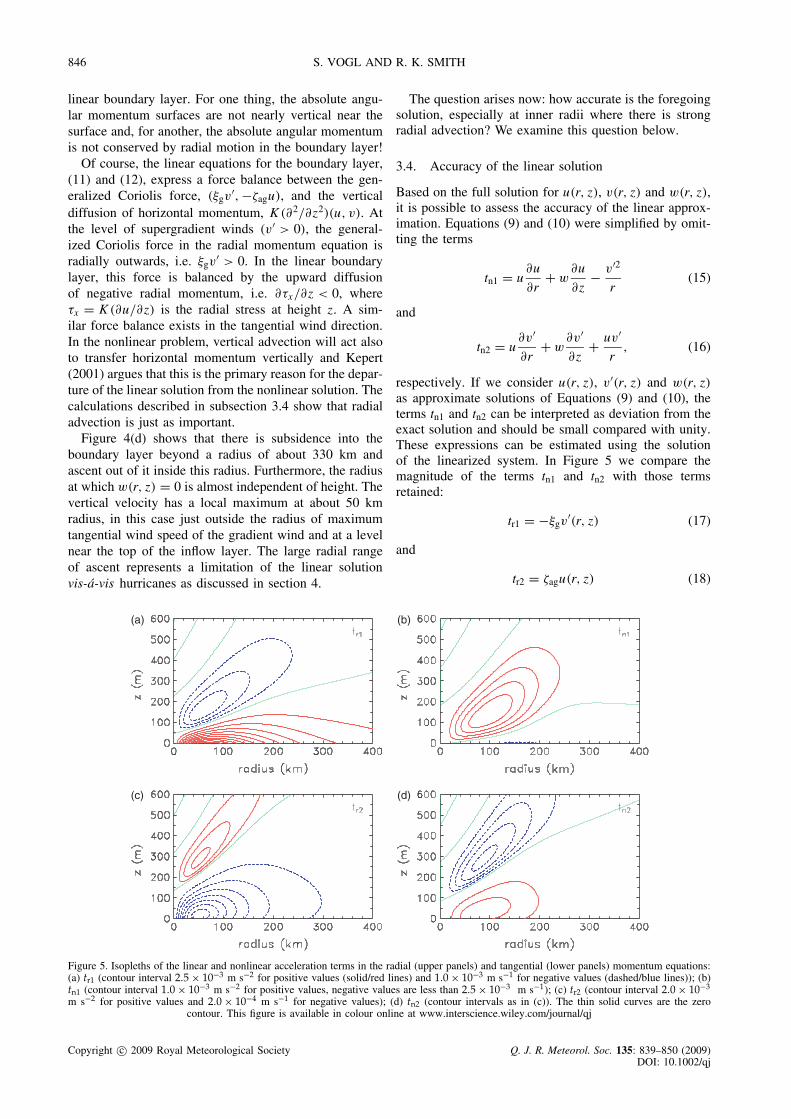
Figure 4(d) shows that there is subsidence into theboundary layer beyond a radius of about 330 km andascent out of it inside this radius. Furthermore, the radiusat which w(r, z) = 0 is almost independent of height. Thevertical velocity has a local maximum at about 50 kmradius, in this case just outside the radius of maximumtangential wind speed of the gradient wind and at a levelnear the top of the inflow layer. The large radial rangeof ascent represents a limitation of the linear solutionvis-a-vis hurricanes as discussed in section 4.

The question arises now: how accurate is the foregoingsolution, especially at inner radii where there is strongradial advection? We examine this question below.

3.4. Accuracy of the linear solution

Based on the full solution for u(r, z), v(r, z) and w(r, z),it is possible to assess the accuracy of the linear approx-imation. Equations (9) and (10) were simplified by omit-ting the terms

tn1 = u∂u

∂r+ w

∂u

∂z− v′2

r(15)

and

tn2 = u∂v′

∂r+ w

∂v′

∂z+ uv′

r, (16)

respectively. If we consider u(r, z), v′(r, z) and w(r, z)

as approximate solutions of Equations (9) and (10), theterms tn1 and tn2 can be interpreted as deviation from theexact solution and should be small compared with unity.These expressions can be estimated using the solutionof the linearized system. In Figure 5 we compare themagnitude of the terms tn1 and tn2 with those termsretained:

tr1 = −ξgv′(r, z) (17)

and

tr2 = ζagu(r, z) (18)

Figure 5. Isopleths of the linear and nonlinear acceleration terms in the radial (upper panels) and tangential (lower panels) momentum equations:(a) tr1 (contour interval 2.5 × 10−3 m s−2 for positive values (solid/red lines) and 1.0 × 10−3 m s−1 for negative values (dashed/blue lines)); (b)tn1 (contour interval 1.0 × 10−3 m s−2 for positive values, negative values are less than 2.5 × 10−3 m s−1); (c) tr2 (contour interval 2.0 × 10−3

m s−2 for positive values and 2.0 × 10−4 m s−1 for negative values); (d) tn2 (contour intervals as in (c)). The thin solid curves are the zerocontour. This figure is available in colour online at www.interscience.wiley.com/journal/qj



respectively. As expected the largest absolute values oftr1 and tr2 occur in a region close to the surface and atinner radii where the radial and vertical gradients of u

and v′ are large (Figure 5(a) and (c)). The correspondingisopleths of the neglected terms, tn1 and tn2, are shownin Figure 5(b) and 5(d), respectively. It is clear that theneglected terms are comparable in magnitude with thoseretained over much of the region of interest. (The fact thatthe zero contours of tn1 and tn2 do not coincide with thoseof tr1 and tr2 makes the comparison in terms of ratios ofthe neglected to retained terms difficult to interpret.)

The foregoing result is consistent with the scale analy-sis in section 2.1. From Table II, the relative importanceof the neglected terms is characterized by the values ofRo� and Ro�, which depend on the chosen profile forvg, together with estimates for Su and Sv′ . In the weakfriction approximation both Su and Sv′ are assumed to besmall compared with unity. Figure 6 shows the parame-ters Su = |u/vg| and Sv′ = |v′/vg| evaluated at the heightsat which the radial wind speed and the tangential winddeficit attain their maximum absolute values for the threevortex profiles shown in Figure 1.

The values obtained for Su and Sv′ are both largestfor vortex 1, with Sv′ reaching a maximum value of 0.3and Su reaching a maximum of 0.83, both at a radius ofabout 285 km. For vortex 2 and vortex 3, the maximaof Su and Sv′ are somewhat smaller and occur at largerradii. In general, the values for Su are not very smallcompared with unity and the highest values do not justoccur in the core region, but cover much of the radialrange shown. This result underpins the findings of thedirect comparison of neglected and retained terms shownin Figure 5. Thus the assumptions of the weak frictionapproximation that Su � 1 and Sv′ � 1 are not valid forall profiles at all radii. The scale analysis in Table II showsthat the nonlinear terms can be neglected if the scales

Figure 6. Ratio of the radial to tangential wind speed Su = |u/vg|(lower three curves) and ratio of the wind deficit to the gradientwind Sv′ = |v′/vg| (upper three curves) evaluated at the height whereu and v′ reach their maximum absolute values for the three vortexprofiles shown in Figure 1. This figure is available in colour online at


Figure 7. Radial profiles of the scales S2uS−1

v′ Ro� (curve a), Sv′ Ro�

(curve b) and Sv′ Ro� (curve c) for vortex 2. This figure is availablein colour online at www.interscience.wiley.com/journal/qj

S2uS

−1v′ Ro�, Sv′Ro� and Sv′Ro� are small compared with

unity. For vortex 2, this is not the case at most radii, asshown in Figure 7, corroborating the conclusions arrivedat above that the linear boundary-layer approximation isinaccurate and does not extend the validity of the classicalEkman layer anywhere near the inner core region of ahurricane.

Kepert (2001, p 2477) stated that ‘. . . a limitationof the linear model is the neglect of vertical advection,which is not supported by a scale analysis’. However,the scale analysis presented in Table II suggests that theneglect of radial advection may be an equally importantlimitation. To examine this feature we calculate theseparate contributions of radial and vertical advectionto tn1 and tn2 in the expressions (15) and (16). Thesecontributions are shown in Figure 8 as functions of radiusat a height of 100 m, at which level the nonlinear termsare a maximum. It is seen that the maximum values of thevertical advection terms are about twice as large as themaximum values of the radial advection terms, but thereare many radii at which the radial advection terms are aslarge as, or even larger in magnitude than, the verticaladvection terms. Evidently the radial advection termscannot be ignored. The third terms in the expressions fortn1 and tn2, i.e. −v′2/r and uv′/r , respectively, are seento be smaller than the corresponding advection terms inthe inner core region.

4. Discussion

The foregoing analysis points to serious limitations of thelinear boundary-layer solution when applied to the innercore of hurricanes, even for radii well beyond the radiusof maximum gradient wind speed. However, there is afurther limitation that we have not yet touched upon. Aspointed out by Smith and Vogl (2008), it is probablyincorrect to prescribe the tangential wind speed just



Figure 8. Radial profiles of the radial and vertical advection terms inthe expressions for (a) tn1 and (b) tn2. In (a), u1 refers to u(∂u/∂r)and u2 to w(∂u/∂z), while in (b) v1 refers to u(∂v′/∂r) and v2 tow(∂v′/∂z). Shown also for comparison are the additional terms in theexpressions, i.e. −v′2/r in tn1 and uv′/r in tn2, which are labelledu3 and v3, respectively. This figure is available in colour online at


above the boundary layer in the inner region, where theflow exits the boundary layer. Many previous boundary-layer models have taken this approach (e.g. Smith, 1968;Ooyama, 1969; Leslie and Smith, 1970; Bode and Smith,1975; Shapiro, 1983; Kepert, 2001; Smith, 2003), butthe consequences thereof have not been investigated ordiscussed in detail. Presumably, with this limitation inmind, Kepert and Wang (2001) used a boundary conditionthat constrains the vertical gradient of the radial andtangential velocity components to be zero at the top oftheir computational domain. Nevertheless, because theradial motion at this boundary turns out to be close tozero (see their Figure 2), the tangential wind speed mustbe close to the gradient wind at this boundary.

We concur with Kepert and Wang (2001) that it is morereasonable to suppose that boundary-layer air carries itsmomentum with it as it ascends out of the boundary layerbecause this boundary is an ‘outflow boundary’ of theproblem. Unfortunately, it is not possible to accommodatea zero vertical-gradient constraint in the analytic solution

of the linear model. Since the radius at which the verticalmotion reverses sign at the top of the boundary layeroccurs relatively far from the vortex centre in the linearmodel, the inability to apply a zero vertical-gradientconstraint further limits the usefulness of the model whenapplied to hurricanes. These remarks apply presumablyto the extension of the linear model to non-axisymmetricflow worked out by Kepert (2001).

As argued by Smith and Vogl (2008), the samelimitation does not exist in a slab boundary-layer modelbecause the boundary-layer wind and gradient wind arenot the same at the top of the boundary layer, eventhough the radial pressure gradient in the boundary layeris the same as that above (see Smith and Montgomery(2008) for a scale analysis for the slab boundary layer).Nevertheless there are still challenging issues involved inproperly coupling a slab boundary layer to the flow above(Smith et al. 2008).

Throughout this article we have assumed the turbulentdiffusivity to be constant with height and radius, afeature that is a gross simplification. We believe that theassumption that the diffusivity is constant with heightis adequate for present purposes when combined with abulk drag formulation of the surface layer (see e.g. Leslieand Smith, 1970; Bode and Smith, 1975). Keeping K

constant with radius is potentially more serious as onewould certainly expect turbulence levels to rise as thewind speeds increase significantly with decreasing radius.Unfortunately observations provide little guidance on themagnitude of this increase. In view of the result that thelinear boundary-layer theory breaks down in the region ofstrong winds, it is questionable whether one would learnmuch more from calculations in which such an increasein K is postulated. Nevertheless, the scaling analysis insection 2.1 suggests that any increase will be reflected in acommensurate increase in the boundary-layer depth abovethat predicted assuming a radially constant K . Similarremarks apply to the representation of the surface dragcoefficient. Here we have used a constant value, whereasobservations suggest that it increases linearly with near-surface wind speed, at least up to wind speeds of about20 m s−1, after which it remains approximately constant(see Black et al. 2006). However the behaviour of CDhas been determined only for wind speeds up to about30 m s−1. We could have used the latest estimates forthe variation of CD in the foregoing calculations, but theadditional degree of sophistication seems unwarranted inview of the limitations of the linear theory that we havedemonstrated.

5. Conclusions

We have derived the boundary-layer equations for a hur-ricane from the Navier–Stokes equations, assuming thatthe turbulent transfer of momentum can be characterizedby a constant eddy diffusivity in conjunction with a bulkrepresentation of surface drag. The derivation is based ona detailed scale analysis of the Navier–Stokes equations.



We showed how a linear form of the boundary-layer equa-tions that has been studied by several previous authors canbe obtained as a weak friction limit of the full equations.The weak friction limit formally assumes that the radialand perturbation tangential velocity components are smallcompared with the gradient wind speed above the bound-ary layer and that the local Rossby number based on theabsolute vorticity of the gradient wind is of order unityor less.

We showed height–radius plots of the three velocitycomponents derived from an analytic solution of thelinear boundary-layer equations. Interesting features arethe presence of supergradient winds at all radii and avertical velocity that has a weak local maximum just atthe top of the inflow layer near the radius of maximumgradient wind speed. The radial profile of vertical velocityat the top of the boundary layer for three tangential windprofiles is similar in shape to those in a slab version ofthe linear model. However, a recent study of the slabmodel has shown that the profiles of vertical velocity inthe linear model are unrealistic compared with that in thenonlinear version. In particular, the radius at which thesubsidence changes to ascent in the linear solution is fartoo large. This would have important ramifications for theintegrity of the linear solution in the continuous model,because the upper boundary condition that the tangentialwind tends to the gradient wind and the radial wind tendsto zero at the top of the boundary layer cannot be justifiedwhen there is ascent out of the boundary layer.

We showed that the linear solution is not self-consistentover a considerable range of radii because the magnitudeof the nonlinear terms calculated from this solution isnot much smaller than the linear terms themselves. Thisconclusion is supported also by considering the relativemagnitude of terms in the scale analysis. These remarksapply presumably also to non-axisymmetric extensions ofthe linear theory.

Acknowledgements

We thank Michael Montgomery for his insightful com-ments on the first draft of the manuscript. Part of thiswork was carried out during a visit by the authors to theNOAA/AOML Hurricane Research Division in Miami.Our thanks go to the Director, Frank Marks, and col-leagues for providing us with a stimulating working envi-ronment. We also thank the two anonymous reviewers fortheir careful reading of the original manuscript and theirconstructive comments on it. The first author gratefullyacknowledges a doctoral stipend provided by the MunichReinsurance Company.

Appendix A: Tangential wind profiles, vg(r)

In the calculations described above we examined a set ofthree profiles for the gradient wind of the form

vg(r) = V1se−α1s + V2se−α2s , where s = r

rm,

where V1, V2, α1 and α2 are constants, chosen so that themaximum wind speed vm is the same (40 m s−1) for eachprofile and occurs at a radius rm = 40 km. In terms of theparameters µ = V2/vm and α2 we can calculate α1 andV1 using

α1 = (1 − µα2e−α2)/(1 − µe−α2),

V1 = vmeα1(1 − µeα2).

}(A1)

The three wind profiles shown in Figure 1 are specifiedby the values for (µ, α): (0.8, 0.4), (0.5, 0.3), and (0.5,0.25). These profiles are all inertially stable (ξgζag > 0)for the Coriolis parameter used (f = 5.0 × 10−5 s−1).

Appendix B: Solution of the linear model

Equations (9) and (10) may be readily solved by elim-inating either u or v′ to give a fourth-order ordinarydifferential equation for the other variable. For example,eliminating u gives an equation for v′:

∂4v′

∂z4+ I 2

K2v′ = 0, (B1)

and then u is given by

u(z) = K

ζag

∂2v′(z)∂z

. (B2)

Kepert (2001) showed that the solution of Equation(B1) that is bounded as z → ∞ has the form

v′(z) = V1e−(1−i)z/δ + V2e−(1+i)z/δ, (B3)

where V1 and V2 are complex constants. This may bewritten in the form

v′(z) = e−z/δ[A1 cos(z/δ) + A2 sin(z/δ)], (B4)

where A1 and A2 are constants determined by a secondboundary condition, e.g. for z = 0. The correspondingsolution for u is obtained by substituting (B4) into (B2),i.e.

u(z) = − 2K

ζagδ2e(−z/δ)[A2 cos(z/δ) − A1 sin(z/δ)]. (B5)

We apply a slip boundary condition at the surface(z = 0) with a quadratic drag law for the surface stress.Defining u = (vg + v′, u) and a drag coefficient CD, thiscondition takes the form

K∂u∂z

= CD|u|z=0 u at z = 0. (B6)

Substituting the expressions (B5) for u and (B4) for v′,we obtain

∂v′

∂z|z=0 = (A2 − A1)

δand

∂u

∂z|z=0 = 2K

ζagδ2

(A1 + A2)

δ.



With

|u|z=0 =√

(vg + A1)2 +

(2K

ζagδ2

)2

A22,

the boundary condition at the surface gives two algebraicequations:

A2 − A1 = ν√

(. . . )(vg + A1),

A2 + A1 = −ν√

(. . . )A2,

}(B7)

where

√. . . =

√(1 + A1

vg

)2

+(

2K

ζagδ2

)2 (A2

vg

)2

and ν = CDRe with Re = vgδ/K . These two equationsmay be solved to calculate the coefficients A1 and A2and to obtain the full solutions (u(r, z), v(r, z), w(r, z))

in terms of the local tangential wind speed at the top ofthe boundary layer, vg(r). The vertical velocity w(r, z) isobtained by integrating the continuity equation (4) withrespect to height to give

w(r, z) = − ∂

∂r

(1

r

∫ z

0ru dz

),

where, using (B5),

∫ z

0ru dz = e−z/δK

δζag

× [(A1 − A2) cos(z/δ) + (A1 + A2) sin(z/δ)].(B8)

References

Black PG, D‘Asaro EA, Drennan WM, French JR. Niiler PP,Sanford TB, Terrill EJ, Walsh EJ, Zhang JA. 2006. Air–sea exchangein hurricanes: synthesis of observations from the coupled boundarylayer air–sea transfer experiment. Bull. Am. Meteorol. Soc. 88:357–374.

Bode L, Smith RK. 1975. A parameterization of the boundary layer ofa tropical cyclone. Boundary-Layer Meteorol. 8: 3–19.

Carrier GF. 1971. Swirling flow boundary layers. J. Fluid Mech. 49:133–144.

Eliassen A. 1971. On the Ekman Layer in a circular vortex. J. Meteorol.Soc. Jpn 49: 784–789.

Eliassen A, Lystadt M. 1977. The Ekman layer of a circular vortex: anumerical and theoretical study. Geophysica Norvegica 31: 1–16.

Emanuel KA. 1997. Some aspects of hurricane inner-core dynamicsand energetics. J. Atmos. Sci. 54: 1014–1026.

Kepert JD, Wang Y. 2001. The dynamics of boundary layer jets withinthe tropical cyclone core. Part II: nonlinear enhancement. J. Atmos.Sci. 58: 2485–2501.

Leslie LM, Smith RK. 1970. The surface boundary layer of ahurricane – Part II. Tellus 22: 288–297.

Miller BI. 1965. A simple model of the hurricane inflow layer. WeatherBureau Technical Note 18-NHRL 75. US Dept of Commerce,National Hurricane Research Laboratory: Miami, Florida.

Montgomery MT, Snell HD, Yang Z. 2001. Axisymmetric spindowndynamics of hurricane-like vortices. J. Atmos. Sci. 58: 421–435.

Ooyama KV. 1969. Numerical simulatoion of the life-cycle of tropicalcyclones. J. Atmos. Sci. 26: 3–40.

Rosenthal SL. 1962. A theoretical analysis of the field motion inthe hurricane boundary layer. National Hurricane Research ProjectReport No 56. US Dept of Commerce, National Hurricane ResearchLaboratory: Miami, Florida.

Shapiro LJ. 1983. The asymmetric boundary layer under a translatinghurricane. J. Atmos. Sci. 40: 1984–1998.

Smith RK. 1968. The surface boundary layer of a hurricane. Tellus 20:473–483.

Smith RK. 2003. A simple model of the hurricane boundary layer. Q.J. R. Meteorol. Soc. 129: 1007–1027.

Smith RK, Montgomery MT. 2008. Balanced boundary layers used inhurricane models. Q. J. R. Meteorol. Soc. 134: 1385–1395.

Smith RK, Vogl S. 2008. A simple model of the hurricane boundarylayer revisited. Q. J. R. Meteorol. Soc. 134: 337–351.

Smith RK, Montgomery MT, Vogl S. 2008. A critique of Emanuel’shurricane model and potential intensity theory. Q. J. R. Meteorol.Soc. 134: 551–561.

Smith RK, Montgomery MT, Nguyen SV. 2009. Tropical cyclonespin up revisited. Q. J. R. Meteorol. Soc. 135: in press. DOI:10.1002/qj.428.


limitations of a linear model for the hurricane ... - lmu

Documents