LIMITATIONS IN THE UNDERSTANDINGOF MATHEMATICAL LOGIC

BY NOVICE COMPUTERSCIENCE STUDENTS

APPROVED BYDISSERTATION COMMITTEE:

Copyright

by

Vicki Lynn Almstrum

1994

Dedication

To the memory of two who loved to learn and loved to teach,

both taken from us before their time:

Lucille A. Almstrum

Louis E. Rosier

LIMITATIONS IN THE UNDERSTANDINGOF MATHEMATICAL LOGIC

BY NOVICE COMPUTERSCIENCE STUDENTS

by

VICKI LYNN ALMSTRUM, B.A. ED, M.A., M.S.

DISSERTATIONPresented to the Faculty of the Graduate School of

The University of Texas at Austin

in Partial Fulfillment

of the Requirements

for the Degree of

DOCTOR OF PHILOSOPHY

THE UNIVERSITY OF TEXAS AT AUSTIN

May, 1994

v

Acknowledgements

The genealogy of research development is a fascinating phenomenon.

Composing this section has allowed me to reflect on the many people who have

influenced my research and the dissertation in diverse ways. I want to begin by

expressing my gratitude to my Committee Members, Nell B. Dale, Ralph W.

Cain, L. Ray Carry, David Gries, and Charles E. Lamb. Each of these gifted

individuals has been a mentor, teacher, and advisor for me; I am grateful for their

time, concern, and support throughout this endeavor.

My initial inspiration for this research can be traced to stimulating

meetings with Jeff Brumfield and Lou Rosier and to interactions with the students

in “my” sections of CS336. I am especially appreciative of the computer science

educators who shared the precious resource of their time (some of them twice!) in

serving as judges at various stages in the content analysis process. Without their

assistance, this study would not have been possible. Listed in alphabetical order,

the judges were Michael Barnett, Richard Bonney, Jeff Brumfield, Debra Burton,

Ken Calvert, Rick Care, Charlotte Chell, Chiung-Hui Chiu, Michael Clancy, Ed

Cohen, Ron Colby, Nell Dale, Ed Deaton, John DiElsi, Edsger W. Dijkstra, Ron

Dirkse, Sally Dodge, Sarah Fix, Ann E. Fleury, Suzy Gallagher, David Gries,

George C. Harrison, Helen Hays, Fran Hunt, Joe Klerlein, Edgar Knapp, Kathy

Larson, David Levine, John McCormick, Nic McPhee, Pat Morris, J. Paul Myers,

Jr., David Naumann, Barbara Boucher Owens, David C. Platt, K. S.

Rajasethupathy, Charles Rice, Hamilton Richards, Lynden Rosier, Dale Shaffer,

vi

Angela B. Shiflet, Angel Syang, Harriet Taylor, Henry M. Walker, J. Stanley

Warford, and Cheng-Chih Wu.

Several people outside of my committee consented to review this

document at various stages during its development. Special “thank you”s go to

Hamilton Richards, Jean Rogers, Chris B. Walton, and Ronald P. Zinke for their

thoughtful and thorough comments. I would like to thank Rick Morgan and Jeff

Wadkins at Educational Testing Services for extensive help at several points

during the course of this study. I am also indebted to Ed Barkmeyer and Brian

Meeks for information about the Language-Independent Datatypes standard as

well as for discussions of other points related to the research. Many others have

contributed important ideas at key points in this process, among them Diane

Schallert, who assigned a psycholinguistics project that shaped the way I

approached the topic; Todd Gross, who brought to my attention a key article from

SIGPLAN Notices; Barbara Dodd, who planted the idea for the content analysis

methodology as well as ideas for other aspects of the study; Pat Kenney, who was

a font of information about ETS; Pat Dickson, who asked many helpful and

pointed statistical questions; and Michael Piburn, who shared information about

the PLT and the use of logic as a predictor of success in science education

research.

The Computer Science Education Seminar at the University of Texas at

Austin has provided a vital forum for exploring ideas within and beyond this

research; I am privileged to meet regularly with such a group. There are

numerous professors and graduate students (former as well as current) at the

University of Texas at Austin, particularly within the Department of Computer

vii

Sciences, whom I thank collectively for their contributions to a stimulating

environment. The experiences I have had through involvement in three NSF-

sponsored workshops prove the value of such programs for fostering the exchange

of ideas among educators and researchers; these workshops were held at SUNY

Stony Brook in 1991 (USE-9054175; Principal Investigator Peter Henderson), at

The University of Texas at Austin in 1992 (USE-9154220; Principal Investigator

Nell Dale), and at Southwestern University in Georgetown, TX in 1993 (USE-

9156008; Principal Investigator Walter M. Potter). The annual SIGCSE

Technical Symposia have also provided important opportunities for professional

growth.

In closing, I want to direct my thanks to family and friends who have

supported and encouraged me through the trials, tribulations, and distractions of

this process. In particular, I want to express my gratitude to my husband, Torgny

Stadler, who has supported my work in countless ways. He is without question

one of the primary reasons I was able to complete and enjoy this great adventure!

viii

LIMITATIONS IN THE UNDERSTANDINGOF MATHEMATICAL LOGIC

BY NOVICE COMPUTERSCIENCE STUDENTS

Publication No._____________

Vicki Lynn Almstrum, Ph.D.

The University of Texas at Austin, 1994

Supervisors: Ralph W. Cain and Nell B. Dale

This research explored the understanding that novice computer science

students have of mathematical logic. Because concepts of logic are at the heart of

many areas of computer science, it was hypothesized that a solid understanding of

logic would help students grasp basic computer science concepts more quickly

and would better prepare them for advanced topics such as formal verification of

program correctness. This exploratory study lays the groundwork for further

investigation of this hypothesis.

Data for the study were the publicly available versions of the Advanced

Placement Examination in Computer Science (APCS examination) and files

containing anonymous individual responses of students who took these

ix

examinations. A content analysis procedure was developed to provide reliable

and valid classification of multiple-choice items from the APCS examinations

based on the relationship between concepts covered in each item and the concepts

of logic. The concepts in the computer science subdomain of logic were clarified

by means of a taxonomy developed for use in this study.

Thirty-eight experts in computer science education were judges in the

content analysis of the multiple-choice items. The judges’ ratings provided

criteria for grouping items into strongly related and not strongly related

partitions. In general, the mean proportion of student respondents that correctly

answered the items in a partition was lower for the strongly related than for the

not strongly related partition, with a smaller standard deviation. The difficulty

distributions for the two partitions were shown to be non-homogeneous (p ≤

.002), with the difficulty distribution for the strongly related partition skewed

more towards the “very difficult” end of the distribution.

The results of this study suggest that novice computer science students

experience more difficulty with concepts involving mathematical logic than they

do, in general, with other concepts in computer science. This indicates a need to

improve the way in which novice computer science students learn the concepts of

logic. In particular, pre-college preparation in mathematical logic and the content

of discrete mathematics courses taken by computer science students need to be

scrutinized.

x

Table of Contents

List of Figures ...................................................................................................... xiv

List of Tables........................................................................................................ xvi

Chapter 1 Introduction.......................................................................................... 11.1 Background ........................................................................................... 11.2 Purpose of the Study.............................................................................. 31.3 Significance of the Study ...................................................................... 31.4 Nature of the Study................................................................................ 51.5 Research Questions ............................................................................... 61.6 Overview of Remaining Chapters ......................................................... 6

Chapter 2 Literature Review................................................................................. 92.1 Mathematical Logic — A Historical Perspective.................................. 92.2 Curriculum Guidelines Related to Logic in Computing ..................... 13

2.2.1 Computer science curriculum guidelines ................................ 132.2.2 Recommendations for discrete mathematics........................... 212.2.3 Guidelines for logic education ................................................ 24

2.3 Mathematical Logic in the Age of Computer Science ........................ 262.3.1 Mathematical logic in programming languages ...................... 262.3.2 Logic as the basis for formal methods..................................... 312.3.3 Logic in discrete mathematics................................................. 35

2.4 The Connection between Logic and Reasoning.................................. 382.4.1 Reasoning skills needed in computer science ......................... 392.4.2 Logic and reasoning in psychological theories ....................... 412.4.3 Logic in Piagetian theory ........................................................ 422.4.4 An instrument for measuring ability in logic and reasoning... 44

xi

2.5 Logic as a Tool for Predicting Success in Science.............................. 462.6 Content Analysis as a Research Methodology.................................... 48

Chapter 3 Research Design................................................................................. 553.1 Identifying Concepts in the Subdomain Logic.................................... 553.2 Identifying a Source of Test Items for Analysis.................................. 583.3 The Content Analysis Procedure......................................................... 61

3.3.1 The taxonomy of concepts as a guideline ............................... 613.3.2 The units to be classified......................................................... 623.3.3 The content analysis classification system.............................. 623.3.4 The judges ............................................................................... 633.3.5 Pilot phase of the content analysis procedure ......................... 643.3.6 Final phase of the content analysis procedure......................... 64

3.4 The Data .............................................................................................. 653.4.1 The ETS data sets.................................................................... 663.4.2 The content analysis data ........................................................ 673.4.3 Partitioning of multiple-choice items...................................... 67

3.5 Analysis of the Data ............................................................................ 693.5.1 Analysis of data in ETS files................................................... 693.5.2 Reliability of the content analysis results................................ 69

3.6 Research Questions and Methods of Analysis .................................... 70

Chapter 4 Findings.............................................................................................. 734.1 Source of Test Items: The APCS Examinations ................................ 73

4.1.1 Composition of the APCS Examinations ................................ 734.1.2 Performance Statistics ............................................................. 74

4.2 Content Analysis Procedure Results ................................................... 774.2.1 The instruments under study ................................................... 774.2.2 The judges ............................................................................... 77

xii

4.2.3 Partitioning the items during the final phase........................... 784.2.4 Content analysis reliability results .......................................... 83

4.2.4.1 Overall reliability ........................................................ 834.2.4.2 Single category reliability ........................................... 844.2.4.3 Individual judge reliability .......................................... 854.2.4.4 Test-retest results for items common to A and AB

versions........................................................................ 874.3 Research Questions and Hypothesis Testing....................................... 89

4.3.1 Descriptive statistics for performance differential betweenpartitions.................................................................................. 89

4.3.2 Differences in difficulty distribution between partitions ........ 914.3.3 Correlation between number correct in partitions................... 95

4.4 Summary of Findings ........................................................................ 1004.4.1 Development of the content analysis procedure.................... 1004.4.2 Comparisons of partitions ..................................................... 101

Chapter 5 Conclusions and Future Research.................................................... 1035.1 Conclusions Regarding Research Questions..................................... 1035.2 Generalizability of Results ................................................................ 1065.3 Suggestions for Future Research....................................................... 107

5.3.1 Continued work with the content analysis procedure ........... 1075.3.2 Development of a diagnostic tool.......................................... 1115.3.3 Approaches to teaching logic to computer science students . 112

5.4 Epilogue............................................................................................. 113

Appendix A Overview of Computing Curricula 1991..................................... 114

Appendix B Topic Outline for the Advanced Placement Examination inComputer Science........................................................................ 120

Appendix C Taxonomy of Concepts in the Computer Science SubdomainTwo-Valued Logic ...................................................................... 124

xiii

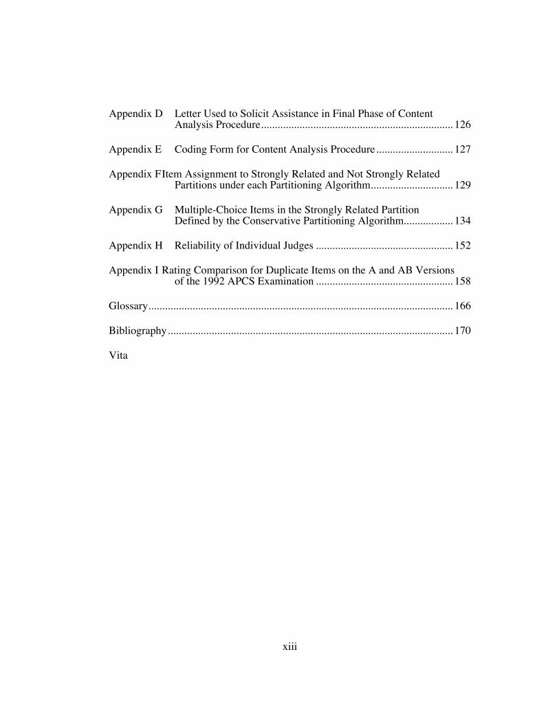
Appendix D Letter Used to Solicit Assistance in Final Phase of ContentAnalysis Procedure...................................................................... 126

Appendix E Coding Form for Content Analysis Procedure............................ 127

Appendix FItem Assignment to Strongly Related and Not Strongly RelatedPartitions under each Partitioning Algorithm.............................. 129

Appendix G Multiple-Choice Items in the Strongly Related PartitionDefined by the Conservative Partitioning Algorithm.................. 134

Appendix H Reliability of Individual Judges .................................................. 152

Appendix I Rating Comparison for Duplicate Items on the A and AB Versionsof the 1992 APCS Examination .................................................. 158

Glossary............................................................................................................... 166

Bibliography........................................................................................................ 170

Vita

xiv

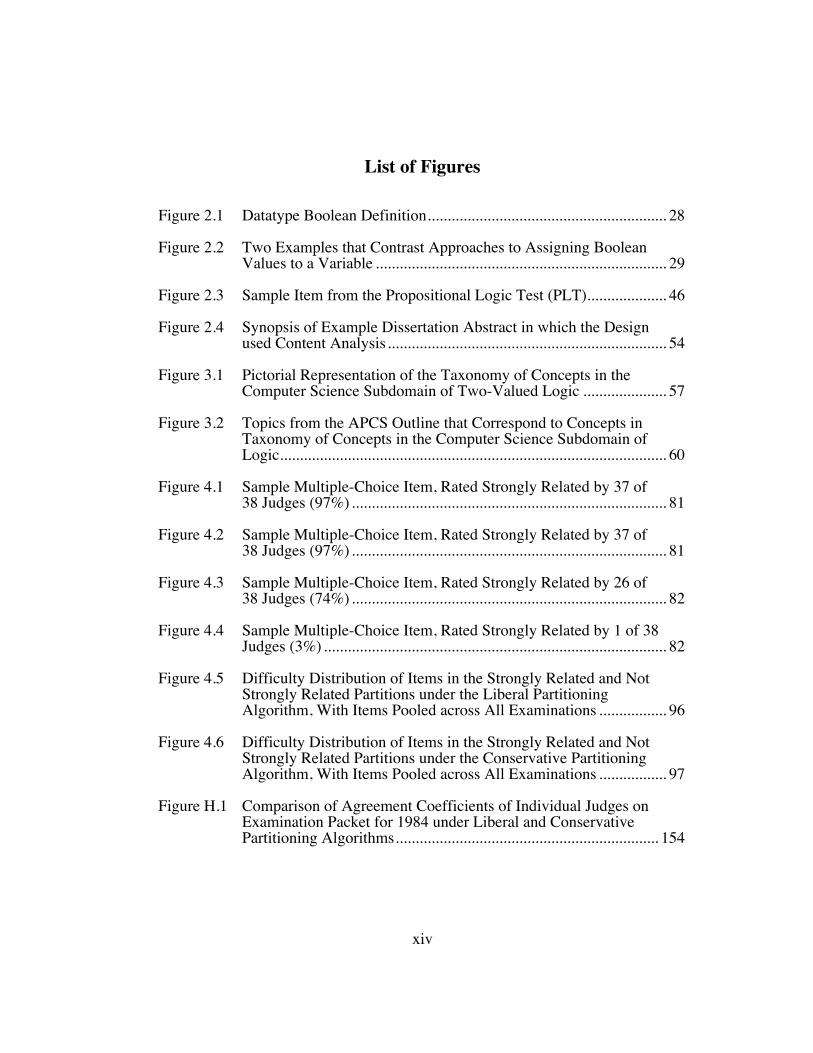
List of Figures

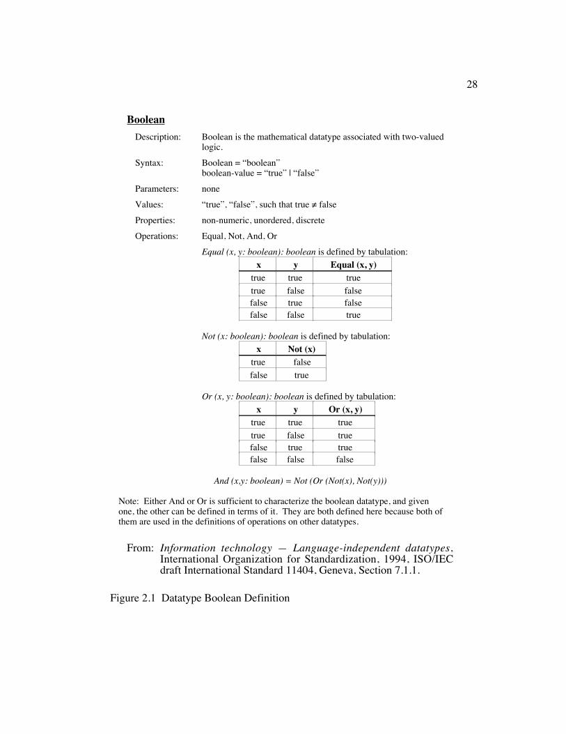
Figure 2.1 Datatype Boolean Definition............................................................ 28

Figure 2.2 Two Examples that Contrast Approaches to Assigning BooleanValues to a Variable ......................................................................... 29

Figure 2.3 Sample Item from the Propositional Logic Test (PLT).................... 46

Figure 2.4 Synopsis of Example Dissertation Abstract in which the Designused Content Analysis...................................................................... 54

Figure 3.1 Pictorial Representation of the Taxonomy of Concepts in theComputer Science Subdomain of Two-Valued Logic ..................... 57

Figure 3.2 Topics from the APCS Outline that Correspond to Concepts inTaxonomy of Concepts in the Computer Science Subdomain ofLogic................................................................................................. 60

Figure 4.1 Sample Multiple-Choice Item, Rated Strongly Related by 37 of38 Judges (97%)............................................................................... 81

Figure 4.2 Sample Multiple-Choice Item, Rated Strongly Related by 37 of38 Judges (97%)............................................................................... 81

Figure 4.3 Sample Multiple-Choice Item, Rated Strongly Related by 26 of38 Judges (74%)............................................................................... 82

Figure 4.4 Sample Multiple-Choice Item, Rated Strongly Related by 1 of 38Judges (3%)...................................................................................... 82

Figure 4.5 Difficulty Distribution of Items in the Strongly Related and NotStrongly Related Partitions under the Liberal PartitioningAlgorithm, With Items Pooled across All Examinations ................. 96

Figure 4.6 Difficulty Distribution of Items in the Strongly Related and NotStrongly Related Partitions under the Conservative PartitioningAlgorithm, With Items Pooled across All Examinations ................. 97

Figure H.1 Comparison of Agreement Coefficients of Individual Judges onExamination Packet for 1984 under Liberal and ConservativePartitioning Algorithms.................................................................. 154

xv

Figure H.2 Comparison of Agreement Coefficients of Individual Judges onExamination Packet for 1988 under Liberal and ConservativePartitioning Algorithms.................................................................. 155

Figure H.3 Comparison of Agreement Coefficients of Individual Judges onExamination Packet for Version A of 1992 Examination underLiberal and Conservative Partitioning Algorithms ........................ 156

Figure H.4 Comparison of Agreement Coefficients of Individual Judges onExamination Packet for Version AB of 1992 Examination underLiberal and Conservative Partitioning Algorithms ........................ 157

xvi

List of Tables

Table 2.1 Mathematics Requirements in Computing Curricula 1991.............. 19

Table 2.2 Piaget’s System of 16 Binary Operations......................................... 45

Table 2.3 Frequency of Subject Categories in Sample of DissertationAbstracts using Content Analysis..................................................... 52

Table 2.4 Component Categories for Two Frequently Reported SubjectCategories in Sample of Dissertation Abstracts using ContentAnalysis............................................................................................ 53

Table 2.5 Source of Data or Method of Generating Data Reported inSample of Dissertation Abstracts Using Content Analysis.............. 54

Table 3.1 Classification System for Indicating Strength of RelationshipBetween APCS Multiple-Choice Items and the SubdomainUnder Study...................................................................................... 63

Table 3.2 Data Used in Study and Source from which Obtained or Derived .. 66

Table 4.1 Summary Statistics for Number of Multiple-Choice ItemsAnswered Correctly on Each APCS Examination ........................... 75

Table 4.2 Descriptive Statistics for Number of Multiple-Choice ItemsAttempted on Each APCS Examination........................................... 75

Table 4.3 Rescaled Descriptive Statistics for Number of Multiple-ChoiceItems Answered Correctly and Number of Multiple-Choice ItemsAttempted on Each APCS Examination........................................... 75

Table 4.4 Summary of Number of Items in Each Partition under EachPartitioning Algorithm for Each APCS Examination ...................... 80

Table 4.5 Agreement Coefficients Showing Overall Reliability of theContent Analysis of the APCS Examinations .................................. 83

Table 4.6 Agreement Coefficients for Single Category Reliability of theFinal Phase of the Content Analysis of the APCS Examinations .... 84

Table 4.7 Comparison of Content Analysis Ratings on Duplicate Itemsfrom A and AB Versions of the 1992 APCS Examination.............. 88

xvii

Table 4.8 Number of Multiple-Choice Items plus Mean and StandardDeviation of Proportion Answering Correctly for AllExaminations.................................................................................... 90

Table 4.9 Number of Multiple-Choice Items, Mean and Standard Deviationof Proportion Answering Correctly, and Delta for Mean andStandard Deviation under Liberal Partitioning Algorithm............... 92

Table 4.10 Number of Multiple-Choice Items, Mean and Standard Deviationof Proportion Answering Correctly, and Delta for Mean andStandard Deviation under Conservative Partitioning Algorithm ..... 92

Table 4.11 Number and Proportion of Items at Each Difficulty Level in theStrongly Related and Not Strongly Related Partitions under theLiberal Partitioning Algorithm......................................................... 96

Table 4.12 Number and Proportion of Items at Each Difficulty Level in theStrongly Related and Not Strongly Related Partitions under theConservative Partitioning Algorithm ............................................... 97

Table 4.13 Correlation between Number Correct in the Strongly Related andNot Strongly Related Partitions under Both PartitioningAlgorithms........................................................................................ 99

Table A.1 Subject Areas Outlined in Computing Curricula 1991 .................. 116

Table A.2 Processes as Defined in Computing Curricula 1991...................... 117

Table A.3 Recurring Concepts as Defined in Computing Curricula 1991...... 118

Table A.4 Knowledge Units Comprising the Common Requirements inComputing Curriculum 1991.......................................................... 119

Table F.1 Number of Judges Choosing Specific Categories for Each Itemand Assignment of Items to Partitions under Each PartitioningAlgorithm for 1984 APCS Examination ........................................ 130

Table F.2 Number of Judges Choosing Specific Categories for Each Itemand Assignment of Items to Partitions under Each PartitioningAlgorithm for 1988 APCS Examination ........................................ 131

Table F.3 Number of Judges Choosing Specific Categories for Each Itemand Assignment of Items to Partitions under Each PartitioningAlgorithm for 1992 APCS Examination, Version A...................... 132

xviii

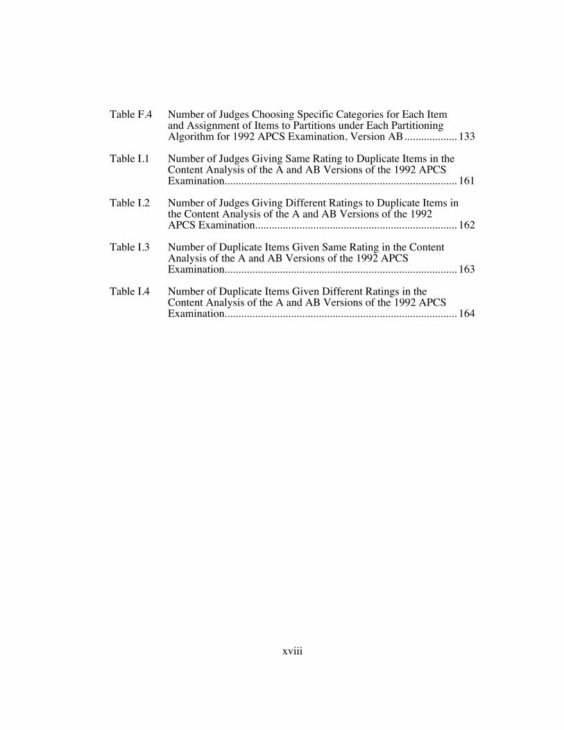
Table F.4 Number of Judges Choosing Specific Categories for Each Itemand Assignment of Items to Partitions under Each PartitioningAlgorithm for 1992 APCS Examination, Version AB................... 133

Table I.1 Number of Judges Giving Same Rating to Duplicate Items in theContent Analysis of the A and AB Versions of the 1992 APCSExamination.................................................................................... 161

Table I.2 Number of Judges Giving Different Ratings to Duplicate Items inthe Content Analysis of the A and AB Versions of the 1992APCS Examination......................................................................... 162

Table I.3 Number of Duplicate Items Given Same Rating in the ContentAnalysis of the A and AB Versions of the 1992 APCSExamination.................................................................................... 163

Table I.4 Number of Duplicate Items Given Different Ratings in theContent Analysis of the A and AB Versions of the 1992 APCSExamination.................................................................................... 164

1

Chapter 1 Introduction

This research explored novice computer science students’ understanding

of mathematical logic (simply referred to as logic in this thesis). Logic restricted

to two values is fundamental to many areas of computer science. Because logic

pervades the field, the investigator hypothesized that a solid understanding of

logic can help students grasp basic computing skills more quickly and can also

prepare them to be more successful when studying advanced topics such as formal

verification of program correctness. The findings and conclusions in this study

establish the baseline for research investigating this hypothesis.

1.1 BACKGROUND

The inspiration for this research arose through the author’s experience as a

teaching assistant in an undergraduate course covering topics in discrete

mathematics and formal verification of computer programs. Each semester, many

students demonstrated a predictable set of misconceptions about and partial

understandings of logic concepts. Because logic is the foundation for formal

verification, these misunderstandings tended to sabotage students’ ability to grasp

the more advanced concepts.

The datatype boolean encompasses a fundamental subset of concepts in

logic that belong to the requisite repertoire of most computer scientists.

Essentially every modern programming language includes the notion of a boolean

datatype and conditional control structures. For example, alternative statements

(such as if-then-else) and repetitive statements (such as while) depend

2

upon a boolean expression that controls which part(s) of the structure will be

executed and how often. Analogous control structures are used in creating

algorithms and specifications.

There is an intricate relationship between the concepts of classic

mathematics and the datatypes that have been included in programming

languages. Because booleans and integers are among the fundamental building

blocks of mathematics, they are included as simple datatypes in most

programming languages. Moreover, these simple types are available on

computers as basic, built-in datatypes complete with their operations. In the

classic textbook Algorithms + Data Structures = Programs, Wirth (1976)

explained: “Standard primitive types are those types that are available on most

computers as built-in features. They include the whole numbers, the logical truth

values, and a set of printable characters” (p. 8). In contrast, while other entities

such as complex numbers and infinite sets are fundamental mathematical

concepts, they are not included as built-in types in programming languages

because there is no effective counterpart available on computers (N. Wirth,

personal correspondence, January 21, 1994).

For many students, working with booleans while learning to program is

their initial formal exposure to the concepts of logic. This research focused on

datatype boolean as representative of the wider subdomain of logic.

3

1.2 PURPOSE OF THE STUDY

This study investigated the question: Do novice computer science

students generally have more difficulty with the concepts of logic than they have

with other areas in computer science? The goals of this study were: (a) to

identify and define clearly concepts in the subdomain of logic; (b) to identify a

method by which relevant material could be isolated from a larger source; and (c)

to provide objective evidence as to whether novice computer science students had

more difficulty understanding the concepts in this subdomain than they had with

the concepts in other novice computer science areas.

1.3 SIGNIFICANCE OF THE STUDY

Many in the computing community have expressed the view that logic is

an essential topic in the field (e.g., Galton, 1992; Gibbs & Tucker, 1986;

Sperschneider & Antoniou, 1991). There has also been concern that the

introduction of logic to computer science students has been and is being neglected

(e.g., Dijkstra, 1989; Gries, 1990). In their article “A review of several programs

for the teaching of logic”, Goldson, Reeves and Bornat (1993) stated:

There has been an explosion of interest in the use of logic incomputer science in recent years. This is in part due to theoreticaldevelopments within academic computer science and in part due tothe recent popularity of Formal Methods amongst softwareengineers. There is now a widespread and growing recognition thatformal techniques are central to the subject and that a good graspof them is essential for a practising computer scientist. (p. 373)

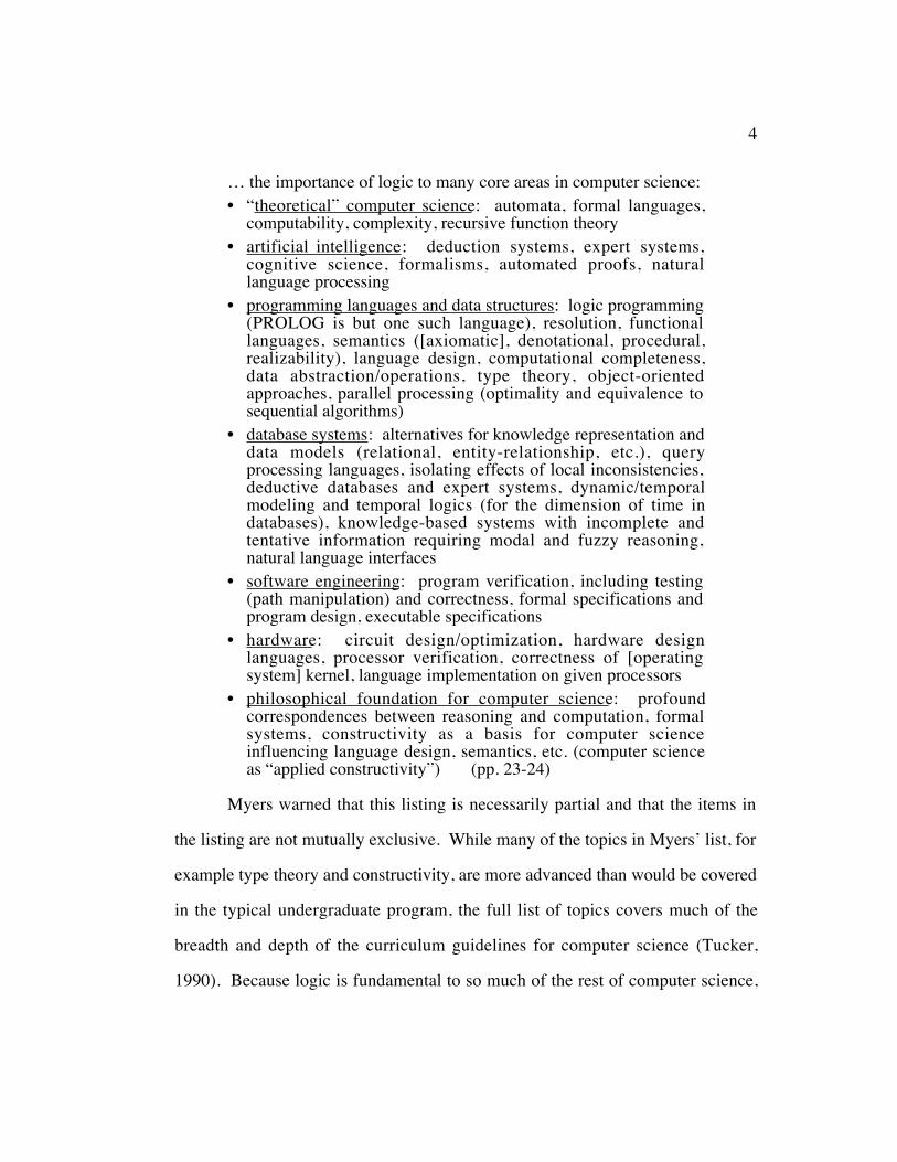
In his paper “The central role of mathematical logic in computer science”, Myers

(1990) provided an extensive list of topics that demonstrate

4

… the importance of logic to many core areas in computer science:• “theoretical” computer science: automata, formal languages,

computability, complexity, recursive function theory• artificial intelligence: deduction systems, expert systems,

cognitive science, formalisms, automated proofs, naturallanguage processing

• programming languages and data structures: logic programming(PROLOG is but one such language), resolution, functionallanguages, semantics ([axiomatic], denotational, procedural,realizability), language design, computational completeness,data abstraction/operations, type theory, object-orientedapproaches, parallel processing (optimality and equivalence tosequential algorithms)

• database systems: alternatives for knowledge representation anddata models (relational, entity-relationship, etc.), queryprocessing languages, isolating effects of local inconsistencies,deductive databases and expert systems, dynamic/temporalmodeling and temporal logics (for the dimension of time indatabases), knowledge-based systems with incomplete andtentative information requiring modal and fuzzy reasoning,natural language interfaces

• software engineering: program verification, including testing(path manipulation) and correctness, formal specifications andprogram design, executable specifications

• hardware: circuit design/optimization, hardware designlanguages, processor verification, correctness of [operatingsystem] kernel, language implementation on given processors

• philosophical foundation for computer science: profoundcorrespondences between reasoning and computation, formalsystems, constructivity as a basis for computer scienceinfluencing language design, semantics, etc. (computer scienceas “applied constructivity”) (pp. 23-24)

Myers warned that this listing is necessarily partial and that the items in

the listing are not mutually exclusive. While many of the topics in Myers’ list, for

example type theory and constructivity, are more advanced than would be covered

in the typical undergraduate program, the full list of topics covers much of the

breadth and depth of the curriculum guidelines for computer science (Tucker,

1990). Because logic is fundamental to so much of the rest of computer science,

5

improving novice students’ skills and understanding in this subdomain can affect

their potential for success within the field as a whole.

1.4 NATURE OF THE STUDY

In this study, the concepts in the computer science subdomain of logic

were described by means of a taxonomy. The taxonomy, in the form of a broad

outline of the concepts in the subdomain of logic, served as the cornerstone of the

rest of the research. By defining the set of concepts under study, the taxonomy

served to focus the research effort.

The data for this research were based on test items and statistics from

several publicly available computer science examinations. The multiple-choice

items on these examinations were studied to identify those items that were

strongly related to logic as well as those items that bore little or no relationship to

logic. In order to accomplish this in a valid and reliable manner, all of the items

from the examinations were classified using the research methodology content

analysis. Experts in computer science education followed a well-defined

procedure to rate each item for how strongly its content was related to the

subdomain of logic. The results of the rating process provided the criteria for

assigning items to partitions on the basis of whether or not they were strongly

related to the subdomain. Comparative analysis of individual performance data

for these items was carried out based on the composition of the partitions.

6

1.5 RESEARCH QUESTIONS

This study sought to provide objective evidence as to whether novice

computer science students have more difficulty understanding concepts in the

subdomain of logic than in understanding other novice computer science

concepts. The first research question that was investigated was:

(a) Can a procedure be developed for reliable and valid classification of

content-area test items according to their degree of relationship to a pre-

defined set of logic concepts?

Given a positive answer to research question (a), the test items under

consideration would be divided into sets of items according to the outcome of the

classification process. The following research questions could then be

considered:

(b) In considering student performance on the test items, was the distribution

of performance different for items whose content was strongly related to

logic than for items whose content was not strongly related to logic?

(c) Was there a relationship between individual performance on the set of

items whose content was strongly related to logic and individual

performance on the set of items whose content was not strongly related to

logic?

1.6 OVERVIEW OF REMAINING CHAPTERS

Chapter 2 reviews related research. Mathematical logic is surveyed from a

historical point of view, laying the groundwork for considering the role of logic in

computer science. Curricular efforts that relate to logic as a subdomain of

7

computer science are reviewed and the use of logic in several areas of computer

science is discussed. The role that logic plays in several psychological theories is

described, followed by an overview of research that has investigated the

connection between ability to use mathematical logic and success in courses in the

natural sciences. Chapter 2 concludes with a brief background on the procedures

of content analysis, including design of the procedures, gathering of the data,

issues of reliability and validity, and a survey of ways in which content analysis

has been used in recent research.

Chapter 3 describes the research design, including the process used in

designing a taxonomy of concepts, motivation for choosing the examinations that

were used as the source of data, the methodology of content analysis followed in

analyzing the examination items, and the algorithms used in partitioning the

examination items into strongly related and not strongly related groupings. The

completed partitioning of items provided the basis for addressing the research

questions posed in Chapter 1. Null hypotheses are developed and the statistical

analyses to be used in considering these hypotheses is described.

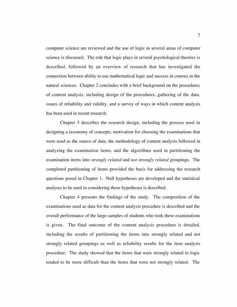
Chapter 4 presents the findings of the study. The composition of the

examinations used as data for the content analysis procedure is described and the

overall performance of the large samples of students who took these examinations

is given. The final outcome of the content analysis procedure is detailed,

including the results of partitioning the items into strongly related and not

strongly related groupings as well as reliability results for the item analysis

procedure. The study showed that the items that were strongly related to logic

tended to be more difficult than the items that were not strongly related. The

8

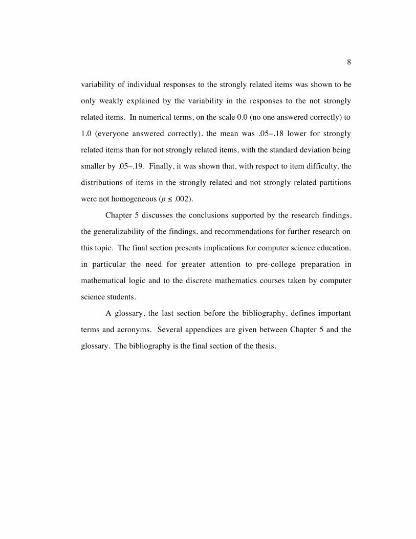
variability of individual responses to the strongly related items was shown to be

only weakly explained by the variability in the responses to the not strongly

related items. In numerical terms, on the scale 0.0 (no one answered correctly) to

1.0 (everyone answered correctly), the mean was .05–.18 lower for strongly

related items than for not strongly related items, with the standard deviation being

smaller by .05–.19. Finally, it was shown that, with respect to item difficulty, the

distributions of items in the strongly related and not strongly related partitions

were not homogeneous (p ≤ .002).

Chapter 5 discusses the conclusions supported by the research findings,

the generalizability of the findings, and recommendations for further research on

this topic. The final section presents implications for computer science education,

in particular the need for greater attention to pre-college preparation in

mathematical logic and to the discrete mathematics courses taken by computer

science students.

A glossary, the last section before the bibliography, defines important

terms and acronyms. Several appendices are given between Chapter 5 and the

glossary. The bibliography is the final section of the thesis.

9

Chapter 2 Literature Review

Chapter 2 begins with a brief historical perspective on the development of

mathematical logic. After a discussion of the status of mathematical logic in

curriculum guidelines in computer science and related fields, the use of

mathematical logic in the age of computer science is explored from the point of

view of programming languages and formal methods. Next, the relationship

between logic and reasoning is considered. Theories about the role of logic and

reasoning in psychology are discussed, followed by a survey of studies that have

investigated the relationship between students’ ability to correctly interpret

propositional logic statements and their success in natural science courses.

Chapter 2 concludes with a discussion of the research technique content analysis

and a review of its use in recent studies.

2.1 MATHEMATICAL LOGIC — A HISTORICAL PERSPECTIVE

The history of logic is closely related to the history of Western

philosophy. As a form of systematic and scholarly inquiry, philosophy was used

by the ancient Greeks (e.g., the pre-Socratics, Plato, and Aristotle) to develop a

set of principles sufficiently comprehensive to account for their knowledge of

both the natural and the human world. With time, the Greek thinkers understood

that for each science there could be a corresponding philosophy of the science.

The philosophy of a science would examine the fundamental principles of the

discipline to see whether they were logical, consistent, and true. Eventually,

philosophical aspects of scientific endeavors were recognized as being distinct

10

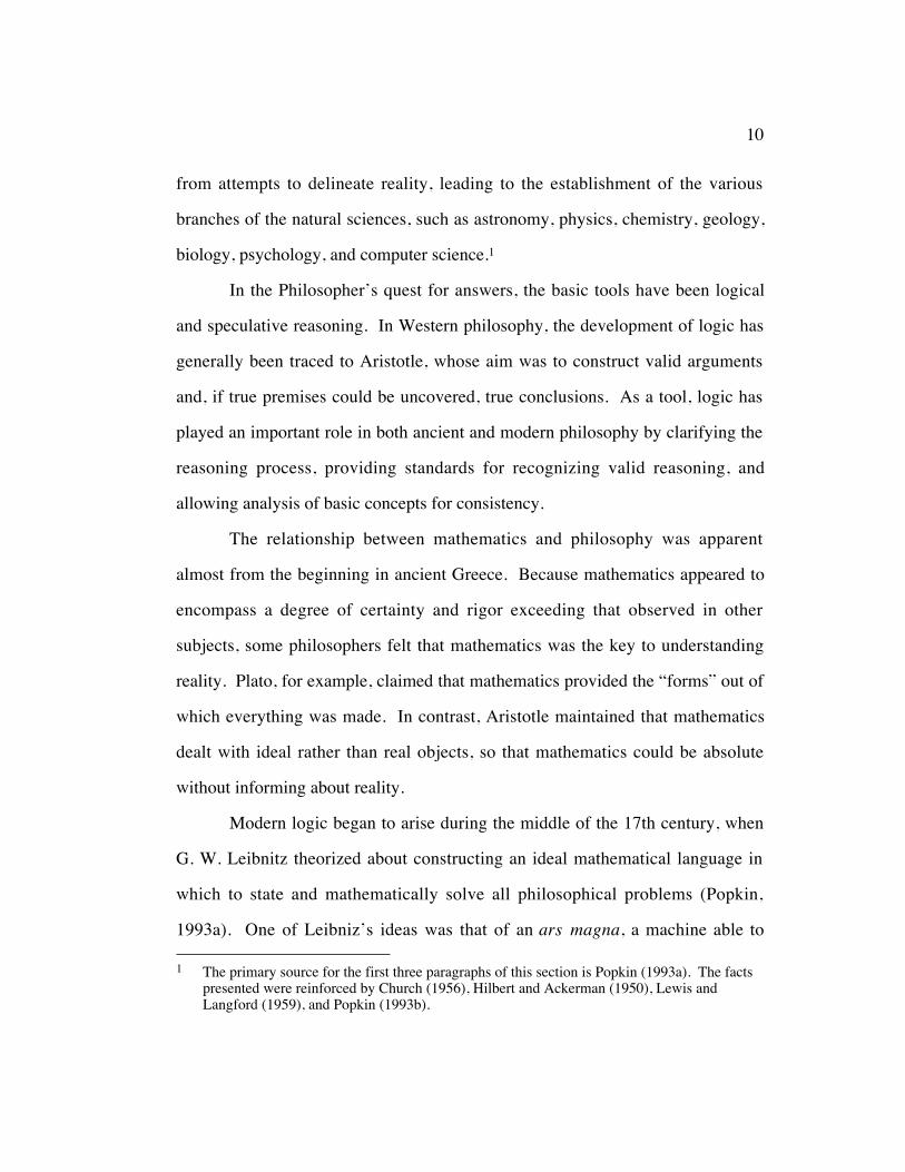
from attempts to delineate reality, leading to the establishment of the various

branches of the natural sciences, such as astronomy, physics, chemistry, geology,

biology, psychology, and computer science.1

In the Philosopher’s quest for answers, the basic tools have been logical

and speculative reasoning. In Western philosophy, the development of logic has

generally been traced to Aristotle, whose aim was to construct valid arguments

and, if true premises could be uncovered, true conclusions. As a tool, logic has

played an important role in both ancient and modern philosophy by clarifying the

reasoning process, providing standards for recognizing valid reasoning, and

allowing analysis of basic concepts for consistency.

The relationship between mathematics and philosophy was apparent

almost from the beginning in ancient Greece. Because mathematics appeared to

encompass a degree of certainty and rigor exceeding that observed in other

subjects, some philosophers felt that mathematics was the key to understanding

reality. Plato, for example, claimed that mathematics provided the “forms” out of

which everything was made. In contrast, Aristotle maintained that mathematics

dealt with ideal rather than real objects, so that mathematics could be absolute

without informing about reality.

Modern logic began to arise during the middle of the 17th century, when

G. W. Leibnitz theorized about constructing an ideal mathematical language in

which to state and mathematically solve all philosophical problems (Popkin,

1993a). One of Leibniz’s ideas was that of an ars magna, a machine able to 1 The primary source for the first three paragraphs of this section is Popkin (1993a). The facts

presented were reinforced by Church (1956), Hilbert and Ackerman (1950), Lewis andLangford (1959), and Popkin (1993b).

11

answer arbitrary questions about the world (Sperschneider & Antoniou, 1991).

His attempts were the first in the history of science to represent logic in the form

of an algebraic calculus (Stolyar, 1970).

Mathematical logic arose from the desire to establish systematic

foundations for the practice of mathematics, for explaining the nature of numbers

and the laws of arithmetic, and for replacing intuition with rigorous proof

(Cumbee, 1993). The foundational crisis of mathematics in the late 19th and

early 20th centuries greatly accounts for the existence of mathematical logic as a

special branch of science (Sperschneider & Antoniou, 1991; Stolyar, 1970).

Modern logic, developed from the 19th century onwards in the work of Boole, de

Morgan, Frege, Jevons, Peano, Peirce, Schröder, Russell, Whitehead, and others,

includes a body of proofs and modes of inference within which the work of

Aristotle and other ancients falls naturally into place, but which in addition

contains a comprehensive theory of relations. The primary difference between

traditional logic and modern logic is that the latter is much more inclusive.

At the beginning of the 20th century, attempts were made to describe

mathematics completely by means of formal systems. One goal was to mechanize

mathematics; this task came to be known by the name Hilbert’s Programme.

Gödel’s work, published in 1931, proved that this task was totally unrealistic by

showing that, for every sufficiently rich formal system, a valid assertion could be

constructed that could not be derived in the formal system. Another fundamental

finding that showed the unfeasibility of Hilbert’s Programme was the famous

undecidability result of Turing and Church (Sperschneider & Antoniou, 1991).

12

The development of modern logic was made possible through the

systematic use of symbolic notation as a medium for formulating even complex

meanings in simple terms (Hasenjaeger, 1972; Stolyar, 1970). Even Aristotle

used letter symbols in logic; however, since no symbolic language had been

developed for mathematics at that time, his use of symbols was very limited.

Formal logic became symbolic when it acquired its own technical language,

essentially an extension of mathematical symbols (Copi, 1979; Stolyar, 1970).

Alfred North Whitehead, an important contributor to the advance of symbolic

logic, highlighted the significance of this progress in his observation that

… by the aid of symbolism, we can make transitions in reasoningalmost mechanically by the eye, which otherwise would call intoplay the higher faculties of the brain. (Whitehead, 1911; cited inCopi, 1971, p. 7)

The extended use of symbolic procedures made the subject of logic broader in

scope and brought logic into new relationships with other exact sciences, such as

mathematics (Lewis & Langford, 1959). Mathematical logic has also been

referred to as symbolic logic, exact logic, formal logic, logistic, and the algebra of

logic (Hilbert & Ackermann, 1950; Lewis & Langford, 1959).

The following quote from Belnap & Grover (1973) concludes this brief

historical perspective on logic by pointing out its widespread utility and the

breadth of applications to which it is applied:

Logic is many things: a science, an art, a toy, a joy. Andsometimes a tool. One thing the logician can do is provide usefulsystems, systems which are both widely applicable and efficient:set theory has been developed for the mathematician, modal logicfor the metaphysician, boolean logic for the computer scientist,syllogistics for the rhetorician; and the first order functionalcalculus for us all. (p. 17)

13

2.2 CURRICULUM GUIDELINES RELATED TO LOGIC IN COMPUTING

Three distinct sources of curricular guidelines address the issue of which

topics of mathematical logic should be included in the education of computer

science students. The first source is the field of computer science. In computer

science-oriented guidelines, logic is not a major focus but is an integral part of

many components of the curricular guidelines. The second source of guidelines

considers logic in the context of the discipline of mathematics. Here, guidelines

cover concepts of logic, but the agenda is broader than mathematical logic. In the

context of this study, recommendations for the discrete mathematics course are of

greatest interest. The third source of guidelines is the mathematical logic

community. Guidelines from this source focus exclusively on the topics of logic

that should be taught, when these topics should be covered, and the subsets of

topics that are important for students in various fields. Throughout this section,

emphasis is on post-secondary education, with pre-college issues discussed as

appropriate.

2.2.1 Computer science curriculum guidelines

As academic disciplines go, computer science is a young field. The first

widely accepted curriculum for academic programs in computer science was

Curriculum '68 (Atchison, 1968), published by the Association for Computing

Machinery; many alternatives and revisions have emerged since then.

In 1982, the Mathematical Association of America (MAA) published

Studies in Computer Science, a book in the series titled Studies in Mathematics

14

(Pollack, 1982a). Studies in Computer Science included nine articles that

provided snapshots of the still-emerging field of computer science. As Pollack

pointed out in the introduction, “… the burgeoning of computer science programs

cannot be equated with the maturation of computer science” (p. vii). The

intention of the volume was to explore computer science as a field distinct from

the various disciplines that used aspects of computing (e.g., numerical analysis).

The first article, “The development of computer science”, was authored by

Pollack (1982b). As part of this historical perspective, Pollack explained how the

very process of defining academic programs for computer science forced

recognition of computing as a discipline separate from others such as mathematics

and engineering. Curriculum '68 in particular acted as a catalyst, providing a

basis for discussion as well as a developmental model for existing and budding

computer science degree programs. However, Pollack (1982) explained that

Curriculum '68

… also had a dichotomizing aspect: Its basically mathematicalorientation sharpened its contrast with more pragmatic alternatives.Most computer science educators agreed that the proposed corecourses included issues crucial to computer science. However, thecurriculum brought to the surface a strong division over the way inwhich these issues should be viewed. In defining the contents ofthe courses, Curriculum '68 established clearly its alignment withmore traditional mathematical studies, giving primary emphasis toa search for beauty and elegance. (p. 41)

During the decade following the introduction of Curriculum '68, a number

of alternative curricula appeared, each in response to objections to Curriculum

'68. According to Pollack (1982), alternative curricula were defined for the areas

of management information systems, software engineering, biomedical computer

science, information science, computing center management, computer

15

engineering, and applied mathematics (with emphasis on the mathematics of

computation).

In the mid-1970s, the ACM initiated a new curriculum effort, intended to

answer the increased demand for professionally-focused computer science

programs. This culminated in Curriculum '78 (Austing, 1979). Curriculum '78

was criticized by many for simply reflecting the status quo in computer science

education, rather than providing a forward-looking model. Berztiss (1987)

observed that, instead of successfully integrating the theoretical and practical

developments that occurred between 1968 and 1978, Curriculum '78 stressed the

practical side of the field and thus lent a vocational spirit to computer science

education. Ralston and Shaw (1980) pointed out that the mathematics

components in Curriculum '78 were essentially the same as those in Curriculum

'68, only weaker: Curriculum '68 required a total of eight mathematics courses,

while Curriculum '78 required only five. Ralston and Shaw predicted that,

because the mathematics of central importance to computer science had changed

drastically during the intervening decade, this would lessen the impact of the

entire report.

A second professional organization for computer science with a deep

interest in curricular issues is the Computer Society of the Institute of Electrical

and Electronic Engineers (IEEE). In 1976 and 1983, the IEEE Computer Society

published model programs in computer science and engineering (IEEE, 1976,

1983). These curricula were specified in the form of subject areas rather than

courses and, for aspects of the curriculum outside of computer science and

engineering, deferred to the standards of the Accreditation Board for Engineering

16

and Technology (ABET). The model program report (IEEE, 1983) described

discrete mathematics as a subject area of mathematics that is crucial to computer

science and engineering. The discrete mathematics course was to be a pre- or co-

requisite of all 13 core subject areas except the first, Fundamentals of Computing,

which had no pre-requisites. The description of the content of discrete

mathematics consisted of detailed lists of topics for eight modules, the first of

which was Introduction to Symbolic Logic. Theoretical concepts listed for this

module were logical connectives, well-formed formulas, rules of inference,

induction, proof by contradiction, predicates, and quantifiers; application concepts

were computer logic and proofs of program correctness. In Shaw’s opinion

(1985), the IEEE program was strong mathematically but was disappointing

because of a heavy bias toward hardware and its failure to expose basic

connections between hardware and software.

An alternative model curriculum, one for a liberal arts degree in computer

science, was described by Gibbs and Tucker (1986). This effort, carried out under

the aegis of ACM, was the product of collaboration of computing educators at

liberal arts colleges who had come to feel that

… the standard set by ‘Curriculum 78’ has become obsolete as aguiding light for maintaining contemporary high-qualityundergraduate degree programs and cannot serve as a basis fordeveloping a new degree program in computer science within aliberal arts setting. (p. 203)

Given the liberal arts setting, the underlying agenda of the curriculum was to

prepare students for a lifelong career of learning. In their description of the model

curriculum, Gibbs and Tucker reaffirmed the view of computer science as a

coherent body of scientific principles. They stressed the essential role of

17

mathematics, “not only in the particular knowledge that is required to understand

computer science, but also in the reasoning skills associated with mathematical

maturity” (p. 207). A discrete mathematics course was recommended as either a

pre- or co-requisite for the second semester computer science course. One

required topic area in the discrete mathematics course was

introduction to logical reasoning, including such topics as truthtables and methods of proof; quantifiers should be included andproofs by induction should be emphasized; simple diagonalizationproofs should be presented. (p. 207)

Other topics of mathematics were described and related to the remainder of the

model curriculum. Mathematical topics that the liberal arts model curriculum

included as “particularly relevant to computer science” were additional areas of

discrete mathematics (e.g., recurrence relations, graph theory, matrices, partially

ordered sets, lattices), calculus (e.g., limits, derivatives, max-min problems,

simple integration), and linear algebra (e.g., vectors, matrix manipulation,

eigenvalues, eigenvectors).

While the ACM and the IEEE curricula were widely used, they became

quickly outdated due to the rate at which the computing field was changing. In

1988, a joint committee of the ACM and the IEEE Computer Society was charged

with the task of defining the discipline of computing. The result of that

committee effort was a document known as the Denning Report (Denning, 1989).

This report became the foundation for an effort to develop computer science

curriculum guidelines suitable for use into the 1990s. A task force with members

from the ACM and the IEEE Computer Society was set up to produce new

guidelines using the Denning Report as a basis. The final report, Computing

18

Curricula 1991 (Tucker, 1990), cited influences of the earlier ACM and IEEE

guidelines as well as of other curricular recommendations produced during the

previous 25 years.

The principles underlying Computing Curricula 1991 included nine

subject areas, three key processes used by professionals in the computing field, a

set of recurring concepts that permeate the topics of computing, and the social

and professional context of the discipline. These principles provided the basis for

defining knowledge units, smaller modules that specify the scope of topics that are

essential for all computing students. Computing Curricula 1991 specifically

avoided the definition of specific courses, recognizing that the wide variety of

institutions and types of programs that existed implied a need for flexibility in

how the subject matter would be mapped to courses. An overview of the subject

areas, processes, recurring concepts, and knowledge units is given in Appendix A.

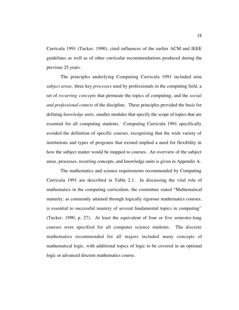
The mathematics and science requirements recommended by Computing

Curricula 1991 are described in Table 2.1. In discussing the vital role of

mathematics in the computing curriculum, the committee stated “Mathematical

maturity, as commonly attained through logically rigorous mathematics courses,

is essential to successful mastery of several fundamental topics in computing”

(Tucker, 1990, p. 27). At least the equivalent of four or five semester-long

courses were specified for all computer science students. The discrete

mathematics recommended for all majors included many concepts of

mathematical logic, with additional topics of logic to be covered in an optional

logic or advanced discrete mathematics course.

19

The Advanced Placement (AP) program, which offers high school

students the opportunity to study college-level material, includes computer

science as a subject area. The AP program, run by the College Board and

administered by Educational Testing Services (ETS), targets three groups:

“students who wish to pursue college-level studies while still in secondary school,

schools that desire to offer these opportunities, and colleges that wish to

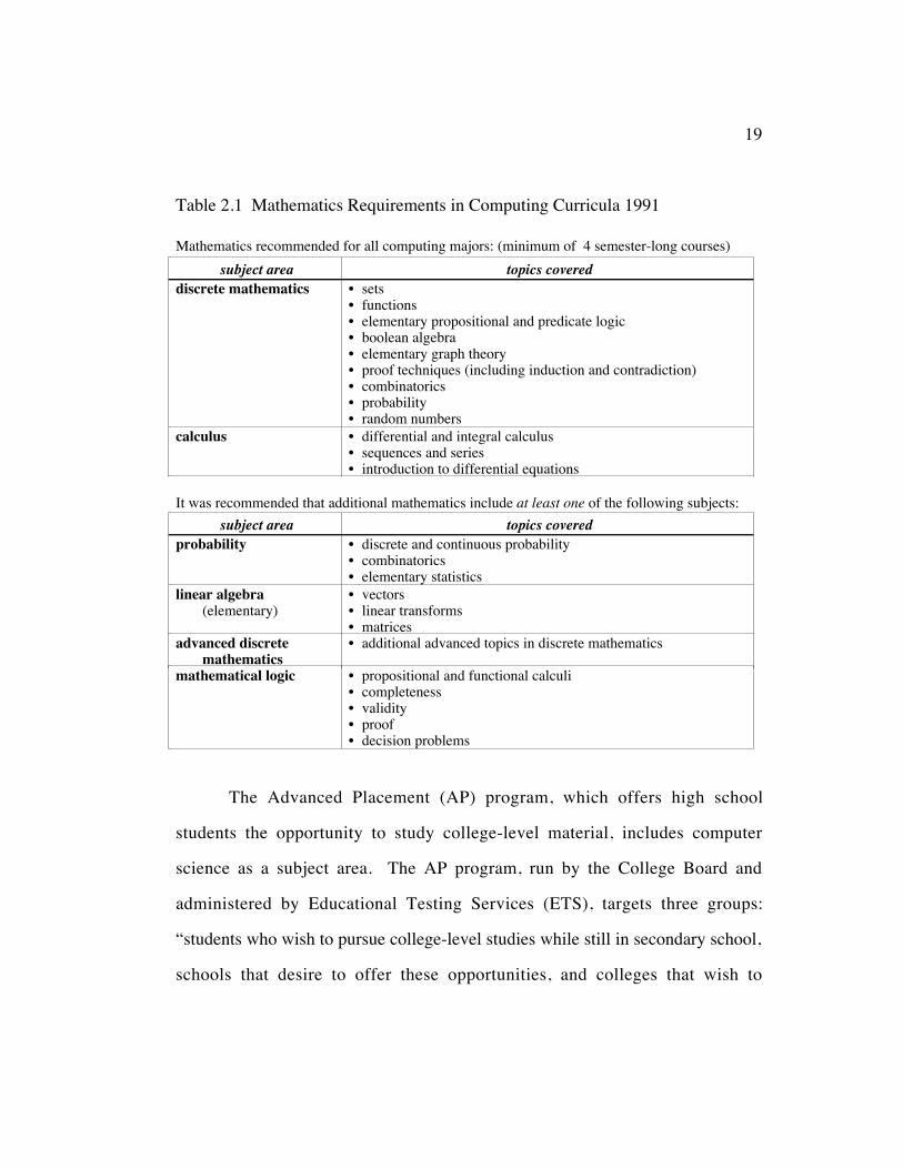
Table 2.1 Mathematics Requirements in Computing Curricula 1991

Mathematics recommended for all computing majors: (minimum of 4 semester-long courses)subject area topics covered

discrete mathematics • sets• functions• elementary propositional and predicate logic• boolean algebra• elementary graph theory• proof techniques (including induction and contradiction)• combinatorics• probability• random numbers

calculus • differential and integral calculus• sequences and series• introduction to differential equations

It was recommended that additional mathematics include at least one of the following subjects:subject area topics covered

probability • discrete and continuous probability• combinatorics• elementary statistics

linear algebra(elementary)

• vectors• linear transforms• matrices

advanced discretemathematics

• additional advanced topics in discrete mathematics

mathematical logic • propositional and functional calculi• completeness• validity• proof• decision problems

20

encourage and recognize such achievement” (College Board, 1990, p. i). The

College Board has defined a topic outline for Advanced Placement in Computer

Science courses, given in Appendix B. The Advanced Placement Examination in

Computer Science is administered annually. Students who take the examination

usually have taken one or more Advanced Placement (AP) courses in computer

science. The items on each AP examination are designed to cover as closely as

possible the topics recommended for the corresponding introductory college-level

course(s). The APCS examination is designed to measure how well students have

learned the requisite concepts of computer science. Students who do well may be

granted placement, appropriate credit, or both by colleges and universities that

participate in the program.

While the APCS program is targeted for college-bound high school

students, the ACM has developed a model computer science curriculum (Merritt,

1993) to address the needs of all high school students. The model curriculum,

which was developed to be consistent with the recommendations in Computing

Curricula 1991, identified essential concepts in computing that every high school

student should understand. The report outlines core, recommended, and optional

topics as the basis for the model; several appendices at the end of the report

describe a variety of possible implementations of the model. While the report

made no specific recommendations for coverage of mathematical logic, one

suggested implementation did address this area. Proulx and Wolf (1993)

presented a set of 12 modules covering the model curriculum topics and, in a

separate table, showed the relationship between the modules and the discrete

mathematics topics given in Computing Curricula 1991 (refer to Table 2.1).

21

Proulx and Wolf explained that the modules covered all but one of the discrete

mathematics topics: the topic of proof techniques was excluded because it was

felt to be inappropriate for high school students.

2.2.2 Recommendations for discrete mathematics

It is generally agreed that students in undergraduate computer science

programs should have a strong basis in mathematics, although there is no

consensus as to what constitutes the appropriate mathematical background. In the

evolution of undergraduate curricula, attempts to recommend which mathematics

courses should be required, the number of mathematics courses, and when the

courses should be taken have been the source of much controversy (e.g., Berztiss,

1987; Dijkstra, 1989; Gries, 1990; Ralston & Shaw, 1980; Saiedian, 1992). A

central theme in the controversy within the computer science community has been

the course called discrete mathematics. Among other topics, the discrete

mathematics course often includes formal logic, the nature of proof, and set

theory.

In 1989, the Mathematical Association of America (MAA) published a

report about discrete mathematics at the undergraduate level (Ralston, 1989).

This report related the experiences of six colleges and universities that were

supported by the Alfred P. Sloan Foundation under a program to foster “the

development of a new curriculum for the first two years of undergraduate

mathematics in which discrete mathematics [would] play a role of equal

importance to that of the calculus” (p. 1). The intention of the Sloan program was

to make recommendations for revision of the first two years of the mathematics

22

curriculum for everyone — mathematics majors, physical science and engineering

majors, social and management science majors as well as computer science

majors. The recommendations put forward by the MAA Committee on Discrete

Mathematics in the First Two Years were as follows:

1. Discrete mathematics should be part of the first two years ofthe standard mathematics curriculum at all colleges anduniversities.

2. Discrete mathematics should be taught at the intellectuallevel of calculus.

3. Discrete mathematics courses should be one year courseswhich may be taken independently of the calculus.

4. The primary themes of discrete mathematics courses shouldbe the notions of proof, recursion, induction, modeling andalgorithmic thinking.

5. The topics to be covered are less important than theacquisition of mathematical maturity and of skills in usingabstraction and generalization.

6. Discrete mathematics should be distinguished from finitemathematics, which, as it is now most often taught, might becharacterized as baby linear algebra and some other topics forstudents not in the “hard” sciences.

7. Discrete mathematics should be taught by mathematicians.8. All students in the sciences and engineering should be

required to take some discrete mathematics asundergraduates. Mathematics majors should be required totake at least one course in discrete mathematics.

9. Serious attention should be paid to the teaching of thecalculus. Integration of discrete methods with the calculusand the use of symbolic manipulators should be considered.

10. Secondary schools should introduce many ideas of discretemathematics into the curriculum to help students improvetheir problem-solving skills and prepare them for collegemathematics. (Siegel, 1989b, p. 91)

With respect to the debate over “calculus vs. discrete mathematics”,

Ralston and Shaw (1980) have observed that

… although we believe strongly that the values of a liberaleducation should infuse any undergraduate program, our focus

23

here is on the professional needs of the computer scientist, not onthe general education needs. Thus, it may be true that all educatedmen and women should be familiar with the essence of calculusbut it does not necessarily follow that computer scientists have asignificant professional need to know calculus. (p. 70)

The alternatives currently considered most viable are: (1) students should enroll

in discrete mathematics and calculus courses simultaneously, (2) calculus should

be delayed until the sophomore or junior year, at which time a more sophisticated

course could be offered because of earlier training in discrete mathematics

courses, and (3) offer a hybrid of calculus and discrete mathematics topics, with

greater emphasis on problem solving and symbolic reasoning (Ralston, 1989;

Myers, 1990).

At the pre-college level, curricular recommendations for discrete

mathematics have been issued by the National Council of Teachers of

Mathematics (NCTM) as part of the Curriculum and Evaluation Standards for

School Mathematics (Romberg, 1989). This document contains a set of

individual standards for pre-college (grades K–12) mathematics curricula. One of

the 14 curriculum standards for high school (grades 9–12) is for discrete

mathematics. The discrete mathematics standard emphasizes that the topics of

discrete mathematics would not necessarily constitute a separate course, but

should instead be integrated throughout the high school curriculum.

Also at the pre-college level, the MAA Committee on Placement

Examinations has attempted to identify skills needed by students taking discrete

mathematics. Siegel (1989b) explained that the committee’s intention was not

necessarily to define an Advanced Placement examination for discrete

24

mathematics but rather to “… help to explain what might be the appropriate

preparation for a successful experience in such a course” (p. 97).

2.2.3 Guidelines for logic education

Yet another view of the topics of logic that should be included in the

educational experience of computing students comes from educators specifically

interested in mathematical logic. The Association for Symbolic Logic (ASL), an

international organization that has been devoted to the study of logic since 1936,

formed an Ad Hoc Committee on Education in Logic in summer 1991. The

committee was charged with making specific recommendations about logic

education for both pre-college and undergraduate programs. Graduate programs

were excluded from consideration because of the diversity of faculty research

interests and of institutional traditions at the graduate level.

The committee’s brief final report (ASL, in press) presents a general view

of concepts in the field of logic with recommendations for the stages at which

various concepts should be introduced. For pre-college students, the stated goal is

to promote and facilitate logical and analytical reasoning at an early age.

Nonspecific strategies are given for different age levels: informal incorporation

of “good” and “bad” arguments for children aged 5–9; heuristic strategies for

(logical) problem solving for children aged 10–13; and the explicit use of logical

notions and techniques for students aged 14–17, probably as part of their

mathematics courses. These recommendations can be contrasted with the NCTM

Standards for School Mathematics (Romberg, 1989). While the NCTM Standards

do not address mathematical or symbolic logic as a separate topic, key concepts of

25

logic are integral to several of the topics. For example, skills such as problem

solving, symbolic manipulation, and reasoning are strongly related to three

themes of the NCTM Standards: mathematics as problem solving, mathematics

as communication, and mathematics as reasoning.

At the beginning post-secondary level, the ASL Guidelines recommend

that all students should be encouraged to take at least one introductory course that

teaches the basic notions of logic, including informal strategies, propositional

calculus, and predicate calculus. The committee noted that such a course could be

taught as a general service course in the philosophy department or as a more

technical course in a mathematics or computer science department. At the

advanced post-secondary level (e.g., at four-year institutions), the ASL Guidelines

advocate an additional set of core topics that are relevant and applicable to many

areas of science and scholarship.

The ASL Guidelines exclude specific course models because of the wide

variety of academic programs and institutions to which the guidelines were

addressed. The ASL report does not relate its recommendations to guidelines in

related fields, such as Computing Curricula 1991 (Tucker, 1990) or the MAA

recommendations for discrete mathematics (Ralston, 1989). The vagueness of the

recommendations and the lack of specific connections to curriculum guidelines in

mathematics and computer science reduce the potential impact of the ASL

Guidelines for Logic Education.

26

2.3 MATHEMATICAL LOGIC IN THE AGE OF COMPUTER SCIENCE

Mathematical logic is pervasive in the field of computer science.

Examples of the breadth and depth of the role of logic have been given by Galton

(1992), Gries and Schneider (1993a), Myers (1990), and Sperschneider and

Antoniou (1991), among others.

Because the uses of logic are so varied and opinions on the role of

mathematical logic in computer science so diverse, this survey has been restricted

to two areas that are closely related to the concepts considered in this study:

programming languages and formal methods for proving program correctness.

2.3.1 Mathematical logic in programming languages

Use and understanding of mathematical logic in programming languages

has centered on datatype boolean. Boolean is a primitive and important datatype

in most computer programming languages.

A broad set of datatypes was defined in the Language-Independent

Datatype (LID) project, which was carried out under the aegis of the International

Standards Organisation (ISO, 1994). In the LID project, each datatype was

defined independent of any particular programming language or implementation.

A goal for the standard was to encourage commonality among and facilitate

interchange of datatype notions between different programming languages and

language-related entities. In the LID standard, each datatype is defined by a basic

set of properties. The ultimate goal was to provide a single common reference

model for all standards that use the concept “datatype”.

27

The formal LID definition of primitive datatype boolean is given in Figure

2.1. The definition gives three properties of datatype boolean: it is non-numeric,

unordered, and discrete. A related datatype defined in the LID standard is

datatype bit, defined as Modulo(2), the two-valued subtype of integer. Although

datatypes boolean and bit resemble one another in many ways, they are distinct

datatypes with different (if analogous) operations. Dijkstra and Feijen (1988)

have admonished “The old-fashioned habit, still found in electrical engineering,

of identifying the values true and false by the integers 1 and 0 respectively must

not be imitated: it only leads to confusion” (p. 43). The separate definitions of

boolean and bit in the LID standard help emphasize this distinction.

Datatype boolean has often been relegated to “second-class citizenship” in

programming languages. Programmers, professionals as well as students, have

tended to use datatype boolean differently than they have used, for example,

datatype integer. For an object to be a first class citizen in a given language, it

must be usable without restriction in whatever ways are appropriate for the

language (D. Naumann, personal communication, November 24, 1993). First, the

datatype should have as its basis a well-defined set of values. For example,

datatype integer has as its basis the set of values {…"–2,"–1,"0,"1,"2,"…}; datatype

boolean is based on the set of values {"true!,"false }. Second, it must be possible

both to evaluate expressions whose result is of that datatype and to assign the

result of expression evaluation to variables of that type. Figure 2.2 gives two

examples from the literature that contrast different ways of evaluating a boolean

expression and assigning the result to a boolean variable. The third requirement

28

BooleanDescription: Boolean is the mathematical datatype associated with two-valued

logic.Syntax: Boolean = “boolean”

boolean-value = “true” | “false”Parameters: noneValues: “true”, “false”, such that true ≠ falseProperties: non-numeric, unordered, discreteOperations: Equal, Not, And, Or

Equal (x, y: boolean): boolean is defined by tabulation:x y Equal (x, y)

true true truetrue false falsefalse true falsefalse false true

Not (x: boolean): boolean is defined by tabulation:x Not (x)

true falsefalse true

Or (x, y: boolean): boolean is defined by tabulation:x y Or (x, y)

true true truetrue false truefalse true truefalse false false

And (x,y: boolean) = Not (Or (Not(x), Not(y)))

Note: Either And or Or is sufficient to characterize the boolean datatype, and givenone, the other can be defined in terms of it. They are both defined here because both ofthem are used in the definitions of operations on other datatypes.

From: Information technology — Language-independent datatypes,International Organization for Standardization, 1994, ISO/IECdraft International Standard 11404, Geneva, Section 7.1.1.

Figure 2.1 Datatype Boolean Definition

29

Example 1The following program statement (2.1) appeared in an algorithm published inCommunications of the ACM (Irons, 1961):(2.1) SW := if INPUT[j] = STAB[i] then true else false

In this statement, a variable of type boolean is being assigned the value of the expressionon the right. Statement (2.1) could be verbalized as “If expression INPUT[j] has thesame value as expression STAB[i], then store the constant value true in variable SW ;otherwise store the constant value false in variable SW ”. This treatment disregards thefact that the expression “INPUT[j] = STAB[i]” has a boolean value — that is, the resultof evaluating this boolean expression is either true or false, depending on the programstate. Thus, statement (2.1) can be rewritten as:(2.2) SW := INPUT[j] = STAB[i]

Example 2Another example of variations in use of datatype boolean is the following warning givenin Jensen and Wirth’s Pascal User’s Manual (1974, p. 27):

If found is a variable of type Boolean, another frequent abuse of the if statement can be illustrated by:

(2.3) if a = b then found := true else found := false

A more parsimonious statement is:(2.4) found := a = b

In this example, statement (2.3) uses an if - then - else control structure to assign one oftwo constants to boolean variable found , while statement (2.4) uses an assignmentstatement to assign the value of a boolean expression to found". In statement (2.3), theoutcome is described via the “control” decisions needed to determine the final value offound ; as the number of conditions increases, the decision structure becomes morecomplex. In statement (2.4), the value of the boolean expression is evaluated and thatresult assigned directly to the boolean variable. As the number of conditions increases,such an expression can be expressed more succinctly than can the corresponding multi-part control structure —and thus the advantage grows.

Note: Program segments are given in Courier font. Reserved keywords such as if ,then , and else are, by convention, underlined. The statement “x := e” assigns theresult of evaluating expression e to variable x. The two-character symbol “:=“ ispronounced “becomes”, “receives the value”, or “is assigned the value of”. The single-character symbol “=” is the infix relational operator for equality.

Figure 2.2 Two Examples that Contrast Approaches to Assigning Boolean Valuesto a Variable

30

for first-class citizenship is that it must be possible to pass arguments and return

function values of the type. (N. McPhee, personal communication, November 22,

1993; D. Gries, personal communication, December 10, 1993).

In their 1988 text A Method of Programming, Dijkstra and Feijen

observed:

For the first 15 years, program execution was understood as acombination of ‘the computation of numbers’ and ‘the testing ofconditions’. While the result of such a (numerical) computationwas formed and stored for later use in the register or memory, theresult of the test of a condition was used immediately (as in analternative statement) to influence the further execution of thecomputation. One merit of Algol 60 was that by introducingvariables of the type Boolean, it was made clear that the testing ofa condition could be better understood as a computation — not asthe computation of a number but as the computation of a ‘truthvalue’. This generalization of the idea of computation is a veryimportant contribution: the proof of a theorem can now beregarded as the demonstration that the computation of aproposition yields the value true. Although we shall only comeacross a modest number of variables of the type Boolean in ourprograms, the type Boolean should not be missing from anyintroduction to programming. (p. 43)

Whether student or professional, programmers’ understanding of fundamental

computer science concepts will be influenced by the features of the programming

language(s) they use. As a result, many programmers fail to benefit from a full

understanding of all of the characteristics of datatype boolean. Algol 60 brought

datatype boolean into first-class citizenship. The programming language C, on

the other hand, allows the programmer to treat boolean as a special case of the

type integer. The confusion caused by such conventions may interfere with

students’ understanding of mathematical logic.

A series of articles and letters published in the professional journal

SIGPLAN Notices illustrates the lack of consensus among practicing professionals

31

regarding the use of logic in computer science (Boute, 1990, 1991; Meeks, 1990,

1991; Nocolescu, 1991; Sakkinen, 1990). SIGPLAN Notices, published by the

ACM Special Interest Group in Programming LANguages, has a readership of

professionals specifically interested in issues surrounding programming language

use, design, and standardization. In 1990, a heated discussion was launched when

Boute (1990) presented his self-proclaimed “heretical” view of datatype boolean

as a subtype of the numeric type natural. Boute’s position was based on a

mathematical argument, which received limited acceptance but was eloquently

rebutted by Sakkinen (1990) and Meeks (1990). Both Sakkinen and Meeks

accepted Boute’s restriction for appropriate situations, but demonstrated that there

were, in fact, many instances where a less restricted view of logic was more

natural and useful. Meeks presented the full range of datatypes related to logic

that were defined as part of the LID standardization effort (ISO, 1994), discussed

earlier. The conclusion drawn by both Sakkinen and Meeks was that, while

Boute’s formulation was valid in its own context and when needed, trying to view

logic purely as a restricted subset of the natural numbers would limit the ability to

express meaning accurately. In other words, if true and false are the notions

being expressed, it is unnecessary, confusing, and restrictive to coerce humans

into translating them into 1 and 0 or some other representation.

2.3.2 Logic as the basis for formal methods

Formal methods encompass a wide range of techniques and languages

used in the development of software. Wing (1990) defined a method as formal “if

32

it has a sound mathematical basis, typically given by a formal specification

language” (p. 8). Cooke (1992) explained:

The term ‘Formal Methods’ alludes to the facility to be able toreason formally (in a mathematically precise, logical way) aboutthe properties of programs and systems. It covers not onlyprogramming languages and the common data types, theiroperators and their properties, but also logic, particularly thenotion of deduction — ‘if something is true then something else istrue’. (p. 420)

Goldson, Reeves, and Bornat (1993) projected the “hope that the use of formal

methods will make programs conform to specification and make them more

reliable but such ‘methods’ are really nothing more than a collection of techniques

imported from discrete mathematics, logic and set theory” (p. 373).

In the article “Logic as a formal method”, Galton (1992) outlined a

representative selection of the ways in which formal logic has been used in

computer science. As applications of classical first-order predicate logic, he

included program specification, program verification, program synthesis, and

logic programming. Beyond classical logic, Galton sketched applications based

on intuitionistic logic, temporal logic, modal logic, and logics for non-monotonic

reasoning. He admitted that, even in his extensive survey, he had neglected many

areas of computing in which logic is important; this serves to punctuate the

breadth of the role of logic in computer science.

This subsection focuses on a specialized area within the range of formal

methods that evolved from work in the formal development of algorithms.

Researchers needed to manipulate formulae of the predicate calculus on a regular

basis yet found that conventional logics, such as natural deduction, required a

great deal of formal detail while providing little or no insight into the

33

development process (Gries & Schneider, 1994). The need for a better model

gave rise to the development of a collection of formal methods referred to as

formal verification of program correctness (where correctness of a program is

established a posteriori) and formal derivation of correct programs (where the

proof of correctness is developed as the program is developed).

Floyd (1967) was the first to suggest that the specification of proof

techniques could provide an adequate formal definition of a programming

language; he also analyzed the potential benefits of using an axiomatic approach

for program proving and for formal language definition. In his seminal paper “An

axiomatic basis for computer programming”, Hoare (1969) acknowledged Floyd’s

suggestion that axioms could provide a simple solution to the problems that arise

when aspects of programming languages are left undefined; whereas earlier

language definitions had been primarily syntactic and in terms of implementation,

axioms made it possible to give a non-operational language definition (i.e.,

independent of implementation). Hoare presented an axiom system in which

programs are expressed as formulae. Such formulae are predicates given in terms

of triples {Q}S{R},2 where S is a statement from the programming language and

Q and R are predicates on the variables used in the statement. Referred to as the

precondition and the postcondition, Q and R describe the initial and final program

states of the statement S. By using axioms and rules of inference that specified

2 This discussion ignores the steps that led from consideration of only “partial correctness” to

“total correctness”. Partial correctness does not address the issue of program termination.Minor notational changes that were a part of this evolution are ignored in favor of the laternotation.

34

the meaning of statements in a simple programming language, it was possible to

verify the correctness of a given program written in that language.

As an alternative to proving the correctness of given programs, Dijkstra

(1968) proposed controlling the process of program generation. In the early

1970s, Dijkstra introduced the notion of predicate transformers as a systematic

way to derive rather than verify programs (Dijkstra, personal communication,

April 14, 1994). The process of program derivation with predicate transformers

was described in Dijkstra’s classic book A Discipline of Programming (1976) and

expanded in the textbook A Science of Programming by Gries (1981). Predicate

transformers extended the Hoare axiom system and provided a means for defining

programming language semantics in a way that would directly support the

systematic derivation of programs from their formal specifications (Dijkstra &

Scholten, 1990). In the Hoare-triple {Q}S{R}, the predicate transformer takes as

arguments statement S and postcondition R; it returns the predicate Q. Q, the

precondition, is a predicate that is satisfied by all of the program states in which

execution of statement S is guaranteed to terminate with predicate R true (Gries,

1981). Stated more succinctly, a predicate transformer is a function of two

arguments, a statement and a predicate, that returns a predicate as its result.

Predicate transformers provide a basis both for deriving correct programs and for

verifying the correctness of existing programs.

Over time, the activities of program verification and program derivation

have become more formal. As limitations in the use of predicate transformers

were encountered, many researchers undertook the task of more formally defining

the theory. Dijkstra and Scholten (1990) explain this process as follows:

35

Probably conditioned by years of formal program derivation, weapproached the task of designing the theory we needed as anexercise in formal mathematics, little suspecting that we wereheading for a few of the most pleasant surprises in our professionallives. After a few notational adaptations of the predicate calculus—so as to make it more geared to our manipulative needs— andthe adoption of a carefully designed, strict format for our proofs,we found ourselves in possession of a tool that surpassed ourwildest expectations. … In the course of the process we profoundlychanged our ways of doing mathematics, of teaching it, and ofteaching how to do it. Consequently, this booklet is probably asmuch about our new appreciation of the mathematical activity as itis about programming language semantics. … As time went on, …we were forced to conclude that the formal techniques we weretrying out had never been given a fair chance, the evidence beingthe repeated observations that most mathematicians lack the toolsneeded for the skillful manipulation of logical formulae. We gave[the tools for manipulating logical formulae] a fair chance; thereader is invited to share our delight. (p. vi)

Dijkstra and Scholten’s efforts resulted in, among other things, an equational

logic. This approach was used informally in the late 1970s and was refined

through the 1980s. In the early 1990s equational logic has come into wider use,

for example in discrete mathematics courses (this will be discussed in the next

section). The key difference between equational logic and other forms of logic is

the extensive use of value-preserving manipulations in the former rather than

proofs composed exclusively of chains of implications.

2.3.3 Logic in discrete mathematics

In his article “Mathematics of computing”, Saiedian (1992) traced the use

of mathematics in computer science through the curricular recommendations

listed in sections 2.2.1 and 2.2.2. He observed that Curriculum '68 explicitly

recommended a computer science course in discrete mathematics, “Introduction

to Discrete Mathematics”. Curriculum '78, which listed the discrete mathematics

36

course “Discrete Structures” as part of the general mathematical requirements,

“did not define explicitly the details of topics to be covered in the course” (p. 208)

and suggested the course as an applied mathematics component that mathematics

departments could provide for computing students. With respect to Computing

Curricula 1991 and the evolving role of the discrete mathematics course, Saiedian

explained:

The recommendations very explicitly recommend a course indiscrete mathematics with a list of all topics to be covered andfurther emphasizes that courses in both advanced discretemathematics and mathematical logic (covering propositional andfunctional calculi, completeness, proofs, etc.) be considered. Aspointed out by a colleague, the Curriculum 1991 view on discretemathematics and mathematical logic represents an “inverted bell-shaped curve” with respect to Curriculum '68 and Curriculum '78.In 1968, discrete mathematics was considered very important whenstudents going into computer science came mostly fromengineering [so that background in] mathematics was no problem.When computing became an area of study for a wider range ofstudents during the 1970s, the emphasis, as reflected in theCurriculum '78, was decreased. However, as the computingdiscipline matured, it became evident that its foundations arestrongly mathematical as shown in the Curriculum 1991. (p. 209)

A wide variety of discrete mathematics textbooks are currently available

for discrete mathematics: In an appendix to the MAA Report on Discrete

Mathematics in the First Two Years, Siegel (1989a) lists 37 textbooks in “A

bibliography of discrete mathematics books intended for lower division courses”.

Siegel admits the list “will surely be out-of-date by the time this book appears” (p.

87); in fact, the list does not include three of the textbooks that were used

regularly in discrete mathematics courses at the investigator’s home institution

from 1988 to 1992. The diversity and number of discrete mathematics textbooks

demonstrates the perceived need for this material.

37

In a comparative review of ten discrete mathematics textbooks, Spresser

and LaTera (1992) used as a benchmark the requirements published by the

Mathematical Association of America (Ralston, 1989; see section 2.2.2). Spresser

and LaTera rated the coverage of formal logic as “very good” for eight of the ten

books. For seven of the ten books, computer science students were listed as part

of, if not the primary, intended audience.

Franzblau (1993) conducted an informal survey of approaches to teaching

discrete mathematics. She presented three course models that she labeled “new”:

(i)"discrete mathematics courses with a focus on proof and (re-)writing,

(ii)"discrete mathematics as the first course for computer science majors, and

(iii)"discrete mathematics courses where logic is used as a tool. For the current

study, the third model is of the most interest. As an example of this model,

Franzblau introduced the approach of Gries and Schneider (1993a, 1993b, 1994).

In Franzblau’s words, they propose “a radically different and highly structured

approach”.

Warford (in press) reviewed Gries and Schneider’s book A Logical

Approach to Discrete Math (1993a) after using it as the text for a discrete

mathematics course he taught. Warford explained that he found that the central

role of the propositional and predicate calculus allowed a unified treatment of

other discrete mathematics topics (e.g., sets, mathematical induction, sequences,

relations, functions, combinatorial analysis, recurrence relations, algebra, graph

theory), as opposed to a “shotgun approach” where the course is made up of

several seemingly unrelated topics. In teaching discrete mathematics using Gries

and Schneider’s approach, Warford found that the character of the course began

38

to resemble that of the traditional calculus: in traditional calculus, students

progress through a series of skill-based exercises such as differentiation, the chain

rule, and integration; in the Gries and Schneider approach to discrete

mathematics, the skill-based exercises include textual substitution, Leibniz’s rule,

boolean expressions, and quantification. In addition, both the traditional calculus

and the logic-based discrete mathematics course have as an underlying theme the

development of students’ skills with proofs and reasoning.

2.4 THE CONNECTION BETWEEN LOGIC AND REASONING

Logic has often been called the science of reasoning. Copi (1971) pointed

out: “As thinking … reasoning is not the special province of logic, but part of the

psychologist’s subject matter as well” (p. 1). For psychologists, reasoning is

interesting from the point of view of process, as a model for human thought; for

logicians, the correctness of the completed reasoning process is of the most

interest. In the field of computing, the use of logic as a tool for expressing and

proving theorems is a key focus.

This section explores connections between mathematical logic and

reasoning. The section begins by exploring the importance of reasoning in

academic success. The role of logic in psychology is discussed, with particular

attention to Piaget’s theory of developmental stages due to both its use of

propositional logic and its major impact on research in this area. Finally, a self-

contained instrument designed to measure skill with propositional logic is

discussed briefly.

39

2.4.1 Reasoning skills needed in computer science

In 1986, Powers and Enright (1987) conducted a survey to determine the

perceptions of a sample of college faculty members about the importance of

analytical reasoning skills for graduate study. Powers and Enright noted,

“Despite the perceived importance of reasoning, there seems to be no consensus

regarding the impact of formal education on the development of reasoning

abilities” (p. 659).

The sample included 255 graduate faculty in six fields of study: chemistry

(N = 37), computer science (N = 43), education (N = 42), engineering (N = 43),

English (N = 44), and psychology (N = 46). Each participant completed a

questionnaire that included items about the importance of various reasoning skills,

including the extent to which each skill seemed to differentiate between marginal

and successful students. The questionnaire also included items about the

importance and frequency of commonly observed errors in reasoning.

Some reasoning skills were consistently rated as very important across the

six disciplines. In decreasing order of rated importance, these skills were:

• reasoning or problem solving in situations in which all the needed

information is not known

• detecting fallacies and logical contradictions in arguments

• deducing new information from a set of relationships

• recognizing structural similarities between one type of problem or theory

and another

40

• taking well known principles and ideas from one area and applying them

to a different specialty

• monitoring one’s own progress in solving problems

• deriving from the study of single cases structural features or principles that

can be applied to other cases

• making explicit all relevant components in a chain of logical reasoning

• testing the validity of an argument by searching for counterexamples

Other skills were rated as important within one discipline but not in others.

For example, “knowing the rules of formal logic” was rated as one of the most

important skills in computer science but was rated as quite unimportant in the

other disciplines. The two reasoning skills that were rated as most important or

critical by the computer science educators were “breaking down complex

problems or situations into simpler ones” and “reasoning or problem solving in

situations in which all facts underlying a situation are known”.

While the underlying reasoning processes are important for academic

success in many disciplines and logic and reasoning are intimately related,

learning about logic is not synonymous with learning to reason. Specifically,

logic is a topic in computing, with underlying skills as important for the student as

the skills of arithmetic. This distinction is important when considering the role of

logic in psychological studies: there is a tendency to blend the two, despite the

differences. As Copi (1979) has stated: “…paradoxically enough, logic is not

concerned with developing our powers of thought but with developing techniques

that enable us to get along without thinking!” (p. 246).

41

2.4.2 Logic and reasoning in psychological theories

Rothaug (1984) surveyed several views of the relationship between formal

logic and the natural psychological logic of thought. The descriptive or rationalist

view held that there is a close relation between logic and reasoning. Another

view held that the laws of logic are only normative and are not useful as a

descriptive model for thinking and reasoning. Piaget and other researchers have

postulated that higher-level psychological processes reflect logical principles, so

that formal logic provides a useful way to characterize a significant component of

thinking and reasoning. Anderson (1980), a cognitive psychologist, viewed the

use of logic as a useful heuristic method for learning about a subject’s behavior

when the subject solves problems (rather than as a model for thinking). Anderson

maintained “Reasoning is fundamentally a matter of problem solving, not a

logical activity … [and] deductive reasoning is a special case of problem solving

rather than some special faculty of the mind” (p. 326). Evans (1980) criticized

research on reasoning on the grounds that previous experiments in this area

involved artificial situations with little relationship to real life situations.

Other views on the role of logic in psychology have been based on the

assumption that human intelligence is not a single trait or process but is instead a

collection of separate abilities. In these models, the ability to do logic is simply

one of many abilities. For example, Guilford (1967) considered a three-

dimensional model of intellect, organized around three main aspects of human

functioning: operations, products, and content. In Guilford’s theory, specific

abilities involve a combination of each of these dimensions. Gardner (1985)

42

argued for the existence of several human potentials, each of which is relatively

autonomous. Gardner hypothesized seven intelligences: logical-mathematical,

linguistic, musical, spatial, bodily-kinesthetic, interpersonal, and intrapersonal;

hence, his theory has been called Multiple Intelligences theory. Gardner and

Hatch (1989) explain that there is not necessarily a correlation between any two

intelligences and that each may entail distinct forms of perception, memory, and

other psychological processes. They characterize the key components of the

logical-mathematical intelligence as “sensitivity to, and capacity to discern,

logical or numerical patterns; ability to handle long chains of reasoning” (p. 6).

2.4.3 Logic in Piagetian theory

Piagetian theory is complex and broad in scope, so it will only be covered

at a very high level in this discussion. Piaget considered intelligence to be the

process of adapting through the cooperating and invariant functions of

assimilation (response based on pre-existing information) and accommodation

(response based on new information). Human development comes about not

because of changes in function but rather due to changes in behavior over time.

Structure describes the properties of intellect that govern behavior, with change

occurring in response to demands of the environment. Schemata are the

structures that allow the mental representation of knowledge; during early life, all

of these schemata are based on physical experience. As humans age, structure is

defined in terms of less overt behavior, characterized by internal activities.3

3 The information in this paragraph and the next was synthesized from discussions by Furth

(1969), Ginsburg and Opper (1979), Inhelder and Piaget (1958), Lefrancois (1988), andStofflett & Baker (1992).

43

With time, thought becomes subject to certain rules of logic, called

operations. In Piaget’s theory, at the pre-operational stage (ages 2–7), thinking is

limited because of the child’s reliance on perception and intuition as well as

egocentric tendencies. At about age seven, the child enters the concrete

operational stage. At this point, the child is able to apply operations to real

objects and events. At the formal operational stage, which Piaget’s findings

showed to begin at about age 12, the child is able to deal with hypothetical

situations and can apply a formal set of logic rules or operations. The child thus

can go beyond empirical reality (the first order operations) to “formal thought”;

the child can now apply second order operations (which use the products of first

order operations). Inherent in formal thought is the ability to perform the 16

operations of propositional logic, outlined in Table 2.2. Inferences are drawn

through applying logical operations to propositions; underlying this is the system

of all possible relations, described by Piaget as the combinatorial system.

Piaget’s theory was for childhood and adolescence, with the formal

operational stage beginning about age 12. However, Petrushka (1984) cites

numerous studies that have shown that a majority of adults, including college

students and professionals, fail at many formal tasks.

Ginsberg and Opper (1979) clarified that Piaget uses logic not to describe

explicit knowledge but to depict the structure of thought, that is: how does logical

thought mediate problem solving? The logical models are not descriptions of

actual performance but are instead abstractions intended to capture the essence of

thought and to allow psychologists to explain and predict behavior. Parsons

(1958) explained that Inhelder and Piaget (1958) used logic as a theoretical tool in

44

describing the mental structures that govern ordinary reasoning and thought. She

pointed out that, while logic is concerned with formalizing internally consistent

systems, psychology deals with mental structures independent of any formal

training or use of symbols and “regardless of consistency or inconsistency, truth

or falsehood” (p. viii). As Furth (1969) pointed out, however, Piaget’s models

were only intended to reflect developing intelligence, which diffuses the

criticisms of the logicians (that the model is not sufficiently sophisticated) and the

psychologist (that the model is too far removed from real thinking).

2.4.4 An instrument for measuring ability in logic and reasoning

The Propositional Logic Test (PLT), developed and used over a number of

years by science education faculty and students at Rutgers University, assesses a

subject’s ability to process propositional statements. In taking the PLT, the

subject is allowed 15 minutes to interpret truth-functional operators by identifying

instances that are consistent or inconsistent with a stated rule (see Figure 2.3 for

an example item). The PLT, which consists of 16 items, can be broken into four

4-item subtests. Each subtest addresses one of the Piagetian operations

conjunction, disjunction, implication, and biconditional. On the PLT, error

patterns are apparent because there are exactly 16 ways that any question could be

answered (i.e., the truth tables of the 16 binary operations of logic as shown in

Table 2.2).

Piburn (1989) has reported that the PLT as a whole has high reliability and

that subtest reliability is best for the biconditional subtest and decreases over the

45

Table 2.2 Piaget’s System of 16 Binary Operations

Piaget’s Disjunctive Normal FormNotation Operation Name p ⁄ q p ⁄

ÿqÿp ⁄

qÿp ⁄ ÿq

o1. PLT: negation

G&O: same F F F F

p ⋅ q2. PLT: conjunction

G&O: same T F F F

p ⋅ q_

3. PLT: non-implicationG&O: inverse of implication F T F F

p_ ⋅ q

4. PLT: non-converse implicationG&O: inverse of converse implication F F T F

p_ ⋅ q

_

5. PLT: conjunctive negationG&O: same F F F T

p [ q ]6. PLT: affirmation of p

G&O: independence of p to q T T F F

q [ p ]7. PLT: affirmation of q

G&O: independence of q to p T F T F

p ≡ q8. PLT: material equivalence

G&O: reciprocal implication T F F T

p » » q9. PLT: exclusive disjunction

G&O: reciprocal exclusion F T T F

q_ [ p ]

10. PLT: negation of qG&O: inverse of #7 F T F T

p_ [ q ]

11. PLT: negation of pG&O: inverse of #6 F F T T

p » q12. PLT: inclusive disjunction

G&O: disjunction T T T F

q … p13. PLT: reciprocal implication

G&O: converse implication T T F T

p … q14. PLT: material implication

G&O: implication T F T T

p / q15. PLT: incompatibility

G&O: same F T T T

p * q16. PLT: tautology

G&O: same T T T T

Note: PLT is the operation name as defined in the key for the Propositional Logic Test,1990; G&O is the operation name as defined by Ginsburg & Opper, 1979, p. 191.

46

implication, conjunction, and disjunction subtests. The PLT has been shown to

correlate highly with grades in natural science courses as well as with the Test of

Logical Thinking (TOLT), another instrument based on Piagetian theory (Tobin

& Capie, 1981). In contrast to other measures of ability with propositional logic,

error patterns on the PLT have revealed systematic relationships between age and

ability that appear to reflect underlying reasoning processes (Piburn, 1989).

2.5 LOGIC AS A TOOL FOR PREDICTING SUCCESS IN SCIENCE

For science educators, the relationship between logic and science is of

special interest because of important parallels between the two: both are systems

that seek truth and the systematic procedures employed by each resemble one

another (Rothaug, 1984). In addition, Rothaug pointed out that, where logic

investigates truth relations between sentences, science seeks to establish in a

systematic way the truth of sentences based on the truth of other sentences .

Science educators have shown that, given their definitions of reasoning and

success, the ability to reason is strongly related to success in science. Stofflett

and Baker (1992) point to results that indicate that students who reason well score

If it is white then it is round.

If it is white then it must be round, but if it is tiled then it doesn’t matter if it is round ornot. So the white circle fits but the white square does not. The tiled figures all fit becausethe statement only tells us about white figures.

Figure 2.3 Sample Item from the Propositional Logic Test (PLT)

47

higher on content examinations, have stronger process skills, and have more

interest in science.

Various studies with students in college physics courses have shown

correlations of .30 to .75 between a variety of measures of logic and achievement

in the course (e.g. Baker & VanHarlingen, 1979; Enyeart, VanHarlingen & Baker,

1980; Lockwood, Pallrand & VanHarlingen, 1980; Pallrand & VanHarlingen,

1980; Piburn & Baker, 1988; Seeber, Pallrand, VandenBerg & VanHarlingen,

1979). Similar results were obtained in studies of high school physics students

(Lockwood, Pallrand & VanHarlingen, 1982) and college chemistry students

(Rothaug & Pallrand, 1982; Rothaug, Pallrand & VanHarlingen, 1981).

The Propositional Logic Test (PLT), described in an earlier subsection,

has been used to measure ability in logic in a number of studies. For example,

Piburn (1990) considered several questions in a study with Australian high school

science students: (1) Is achievement in science positively correlated with ability

to reason about logical propositions? (2) Are some logical operators more

strongly related to achievement in science than others? (3) Is reasoning about

logical propositions related to sex or ability level? (4) Are patterns of error on a

test of the ability to reason about logical propositions related to ability?4 Piburn

found that the coefficient of correlation between final grade in science and

success on the PLT for the entire sample was .57. He also considered subtest

correlations for conjunction, disjunction, implication, and biconditional. He

found that advanced students received the highest scores and basic students the 4 In the Australian school system, students are tested and, based on their scores, classified into

ability groups as advanced (top 25%), basic (bottom 25%) or intermediate (the middle 50%)(Piburn, 1990).

48

lowest, with the greatest difference showing up between advanced and

intermediate students. Piburn discovered that the pattern of errors on subtests

across ability groups in the Australian sample was the same as that across grade

levels in cross-sectional studies of American students from grades 7 to the first

year in college. Piburn found that correlations between the score on the PLT and

achievement in science were significant and relatively high for both the

Australian and American samples.

Stager-Snow (1985) designed a study in which the subjects were students

in an introductory computer science course for non-computer science majors. Her

results indicated that for the females in the sample the PLT was a weak predictor

variable; for the males, the PLT had no predictive power. In addition, Stager-

Snow found that knowledge of the if-then statement contributed more to the

variance in explaining computer knowledge for the females than for the males.

2.6 CONTENT ANALYSIS AS A RESEARCH METHODOLOGY

In its simplest form, content analysis is a technique for making replicable

and valid inferences from textual data to their context. It is frequently used in the

social sciences, especially for the purpose of analyzing communications such as

newspaper articles or textbooks. As an example, suppose that a researcher was

interested in studying the use of symbols and language in messages posted on

electronic bulletin boards for the strategic use of humor. Using content analysis,

the investigator could evaluate occurrences of textual figures, icons (e.g., the

smiley face :-)), and phrases (e.g., parenthetical remarks such as (wink,

wink)) for intent to express humor.

49

Content analysis is exploratory, fundamentally empirical in orientation,

and predictive in intent (Krippendorff, 1980). As a methodology, content analysis

enables the researcher to plan, to communicate, and to critically evaluate the

research design independently of the results. Content analysis provides a basis for

making inferences through the systematic and objective classification of specified

characteristics within a text (Stone, Dunphy, Smith, & Ogilvie, 1966). In the

current study, the characteristics of interest were the concepts of logic; the text

under consideration was the examination(s) to be analyzed; and the inferences

were made by individuals serving as judges, who used a four-category

classification system to rate examination items for their relationship to logic.

When designing a content analysis study, the researcher must identify both

the phenomena to be studied and potential sources of data. Any content analysis

includes two kinds of reality, “the reality of the data and the reality of what the

researcher wants to know about” (Krippendorff, 1980, p. 170). Since the two

realities seldom map directly onto one another, the researcher must discover ways

to analyze the available data so they are indicative of the phenomena of interest.

Given a universe of appropriate data, the researcher must define:

• a sampling plan (e.g., every third book from a randomly ordered list of

books),

• a method for breaking each sample into units (e.g., words, sentences,

paragraphs, or chapters), and

• a coding or classification system that will be used to record information

about the units.

50

While content analysis can be conducted by a single individual, usually it

involves two or more coders or judges. As a means for anticipating and solving

problems, testing and training are vital aspects of the planning process. Because

insight gained during the design and training process may point out problems or

better approaches, the design process will be iterative. Problems such as

inconsistencies or missing records can emerge even in carefully planned studies.

The content analysis proper begins only after the procedure is stable.

During the analysis phase, the researcher must evaluate the coding results

for reliability and validity. Reliability techniques in content analysis are targeted

toward evaluating agreement among judges and ratings. Several types of

reliability can be calculated: overall reliability of the content analysis, item

reliability (how consistent were the judges in rating the particular item?), single

category reliability (how consistently was the content analysis classification

system used?), and judge reliability (how well did each judge agree with the

remaining judges?).

In content analysis, the issue of validity is related to external validity;

internal validity is simply another term for reliability. External validity concerns

two phenomena: 1) how well the findings reflect the true phenomena in the

context of the data, and 2) whether there is a correspondence between variations

within the analysis process and variations that exist outside of the process.�

This section concludes with an informal survey of studies that have used

content analysis in their design. The source of this information is the dissertation

abstracts reported in the ProQuest Dissertation Abstracts On Disc (January,

51

1993–February 1994). This survey is essentially a content analysis of the

abstracts.

A keyword search using the phrase “content analysis” matched 362

dissertation abstracts in the database. Of these, six were eliminated from

consideration because they described research in the natural sciences; in these

studies, the content being analyzed was physical phenomena such as hair, water,

or digestive tract. Of the remaining 356 abstracts, 111 were for degrees awarded

in 1993, 211 were for 1992, 26 were for 1990, four were for 1990, three were for

1989, and one was awarded in 1984.

An average of 2.32 subject categories were listed for each abstract (a

maximum of three subject categories could be given for an abstract). Table 2.3

summarizes the subject categories ordered by frequency of citation. Table 2.4

shows the breakdown into component categories of two of the most frequently

named categories, Education and Psychology. These categories were chosen as

examples for their close connections to the current study. Table 2.5 summarizes

the data collection techniques that were used in the abstracts. Figure 2.4 is the

synopsis of an example abstract related to the field of computer science (Murfin,

1993).

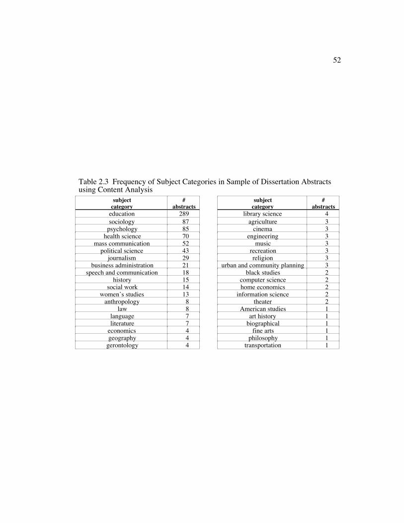
52

Table 2.3 Frequency of Subject Categories in Sample of Dissertation Abstractsusing Content Analysis

subjectcategory

#abstracts

subjectcategory

#abstracts

education 289 library science 4sociology 87 agriculture 3

psychology 85 cinema 3health science 70 engineering 3

mass communication 52 music 3political science 43 recreation 3

journalism 29 religion 3business administration 21 urban and community planning 3

speech and communication 18 black studies 2history 15 computer science 2

social work 14 home economics 2women’s studies 13 information science 2

anthropology 8 theater 2law 8 American studies 1

language 7 art history 1literature 7 biographical 1

economics 4 fine arts 1geography 4 philosophy 1

gerontology 4 transportation 1

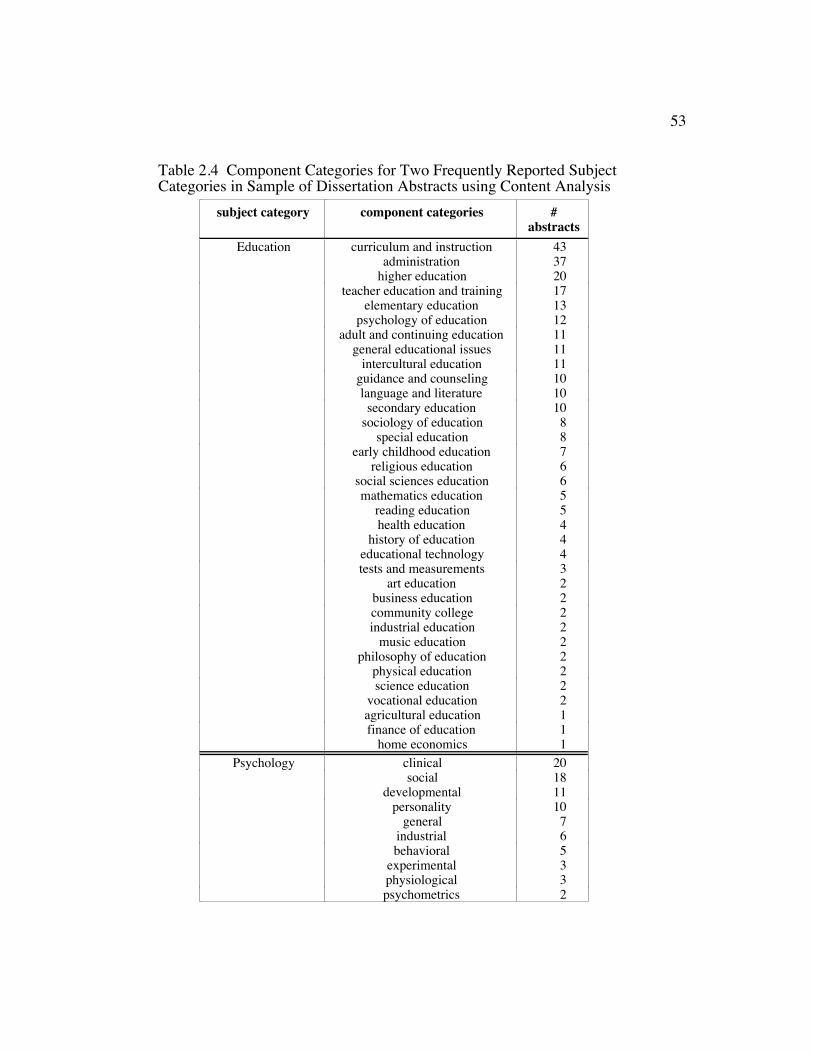
53

Table 2.4 Component Categories for Two Frequently Reported SubjectCategories in Sample of Dissertation Abstracts using Content Analysis

subject category component categories #abstracts

Education curriculum and instruction 43administration 37

higher education 20teacher education and training 17

elementary education 13psychology of education 12

adult and continuing education 11general educational issues 11

intercultural education 11guidance and counseling 10language and literature 10secondary education 10

sociology of education 8special education 8

early childhood education 7religious education 6

social sciences education 6mathematics education 5

reading education 5health education 4

history of education 4educational technology 4tests and measurements 3

art education 2business education 2community college 2industrial education 2

music education 2philosophy of education 2

physical education 2science education 2

vocational education 2agricultural education 1finance of education 1

home economics 1Psychology clinical 20

social 18developmental 11

personality 10general 7

industrial 6behavioral 5

experimental 3physiological 3psychometrics 2

54

Table 2.5 Source of Data or Method of Generating Data Reported in Sample ofDissertation Abstracts Using Content Analysis

source of data /method of generating data

#abstracts

source of data /method of generating data

#abstracts

official document 125 electronic communication 5interview 98 magazine 4newspaper 36 reference book 3

questionnaire 21 visual (photographs) 3television 16 arts (e.g. dance) 2

article 16 field notes 2textbook 14 film 2survey 13 paper & pencil instrument 2

literature 11 journal/reflective writing 2discourse 9 music 2

observation 8 radio 1advertising (magazine or TV) 6 speech 1

Title : An Analysis of Computer-Mediated Communication between Urban MiddleSchool Students and Scientists (Urban Education)

Author : Murfin, Brian EdwardSchool : The Ohio State UniversityDegree : Ph.D.Date : 1993Source : DAI-A 54/05, p. 1770, Nov 1993.Subject categories : education, technology

education, sociology ofcomputer science

Purpose of study : determine the characteristics of effective and ineffective computer-mediated communication between urban middle school students and scientists.

Sample : 20 urban, middle school students and 10 adult scientists and non-scientists.Units of study : An electronic bulletin board system (BBS) was used to link the scientists

and students; 911 messages were posted on the BBS over a 10 week period.Conclusions : content analysis of all messages revealed, among other things:

(1) the number of positive messages was greater than the number of neutral ornegative messages

(2) the students mainly sent messages to only one individual and did not takeadvantage of the multiloguing [i.e., multiple people in dialogue] capability ofcomputer-mediated communication

(3) non-science messages were more numerous than were science messages.

Figure 2.4 Synopsis of Example Dissertation Abstract in which the Design usedContent Analysis

55

Chapter 3 Research Design

Chapter 3 presents the research design, elaborating, in the process, the

research questions posed in Chapter 1. This study was exploratory and

descriptive in nature. Preparatory activities included development of a taxonomy

of relevant concepts and identification of appropriate computer science materials

for analysis. Using a content analysis procedure, expert judges rated multiple-

choice items using a four-category classification system. The classification

system allowed each judge to indicate the degree of relationship between an item

and the subdomain criteria (the taxonomy of concepts). The data that resulted

from content analysis were used in two distinct analyses: (a) use of the strength

ratings to assign the items to strongly related and not strongly related partitions

and (b) determination of the reliability of the content analysis results. The

partitions of items provided the basis for answering the research questions

comparing performance data across the partitions.

3.1 IDENTIFYING CONCEPTS IN THE SUBDOMAIN LOGIC

The investigator developed a taxonomy of concepts to provide a concrete

definition of concepts in the computer science subdomain of mathematical logic.

The taxonomy outlined logic concepts that were particularly relevant to this

research, thus focusing the subsequent research effort on a well-defined set of

concepts.

56

The development of the taxonomy was an iterative process influenced by a

wide variety of sources, including standard computing curriculum guidelines

(e.g., Austing, 1979; Koffman, Miller, & Wardle, 1984; Koffman, Stempel, &

Wardle 1985; Tucker, 1990), the way in which the concepts were presented in

undergraduate textbooks (e.g., Dale & Walker, in press) and more advanced texts

(e.g. Gries, 1981; Sperschneider & Antoniou, 1991), and the draft of an

international standard for datatypes (ISO, 1994). During its development, the

taxonomy was reviewed by several computer science educators to ensure its

content validity.

The resulting taxonomy is a broad outline that provides a breakdown of

advanced as well as basic concepts of logic. The taxonomy was labeled as

containing concepts in the computer science subdomain “two-valued logic” in

order to emphasize the sort of logic that was under consideration in the content

analysis procedure.

As a pictorial synopsis of the concepts belonging to the subdomain of

interest, the Quick Reference to the Concepts of “Two-Valued Logic” was

designed to aid the judges in completing the classification task. Figure 3.1 is the

quick reference guide that was provided to each judge who participated in the

final phase of the content analysis procedure. The full taxonomy is given in

Appendix C.

57

Figure 3.1 Pictorial Representation of the Taxonomy of Concepts in theComputer Science Subdomain of Two-Valued Logic

58

3.2 IDENTIFYING A SOURCE OF TEST ITEMS FOR ANALYSIS

This research depended on having a source of test items for which:

(a) the content tested by the examination covered beginning computer science

concepts, including concepts in the subdomain of logic;

(b) the content of the examination items could be analyzed for strength of

relationship to the concepts of logic;

(c) a sufficiently large sample of students had taken the examination(s) from

which the items were drawn; and

(d) performance information was available for the sample.

The publicly available Advanced Placement Examinations in Computer Science

(APCS examinations) appeared to meet all of these criteria. Because several

thousand students take the examination each year, statistics about the examination

outcome provide a broad base of information about the performance of novice

computer science students.

The College Board’s APCS examination is designed to test the material

covered during the first two courses of the post-secondary computer science

curriculum, generally referred to as “CS1” and “CS2” (Austing, 1979; Koffman,

Miller, & Wardle, 1984; Koffman, Stempel, & Wardle 1985). The full topic

outline for APCS courses is given in Appendix B. Figure 3.2 summarizes the

topics from the APCS outline that most nearly match those in the taxonomy of

logic defined for this research. This extract is somewhat generous, in that it

59

includes several topics that will sometimes be related to logic, rather than topics

that are only related to logic.

Each of the APCS examinations was made up of two parts, a multiple-

choice section and a free-response section. Each multiple-choice section included

from 35 to 50 items while the free-response section included three or five items.

A multiple-choice item comprised a problem statement and five alternative

responses, one of which was correct. Each free-response item presented a

problem description or specification for which the respondent was to write all or

part of an algorithm or computer program. Scoring of the multiple-choice items

was done using a mechanical scanning and scoring system. The free-response

section was scored manually by teams of computer science educators using

scoring rubrics.

Due to the laws in several states, the free-response items must be made

publicly available annually. However, ETS is only required to disclose the

multiple-choice questions every fourth year. As a result, the full APCS

examinations were available for the years 1984, 1988, and 1992. For each of

these three years, Educational Testing Services (ETS) published a report that

included the full text of all items, the correct answers for the multiple-choice

section, grading rubrics for the free-response items, and selected statistical

analyses (College Board, 1986, 1989, 1993).

Files obtained from ETS included anonymous individual data for all

candidates taking the examinations under consideration. For each respondent, the

following information was included: demographic information (gender and

60

ethnicity), response to each multiple-choice item, the score on each free-response

item, and overall APCS grade.

While the sampling represented by the APCS examinations was extensive,

it was also self-selective. Only some students took the classes that prepared them

to take the examination and, of these students, only some chose to take the APCS

examination. Due to the stated purpose of the AP program, a majority of the

students who took the examination were college-bound (College Board, 1990).

A. Programming methodology1. Specification

b. Program and subprogram specifications(e.g., pre- and postconditions)

2. Design3. Implementation

b. Program correctness i. Testing and debugging

A. Reasoning about programsB. AssertionsC. Invariants

ii. VerificationB. Features of block-structured programming languages

1. Type and constant declarationsb. Simple data typesc. Structured data types

3. Expressions and evaluation4. Assignment statements5. Control structures

b. Conditional executionc. Loops

7. SubprogramsC. Fundamental data structures

Figure 3.2 Topics from the APCS Outline that Correspond to Concepts inTaxonomy of Concepts in the Computer Science Subdomain of Logic

61

The APCS data used in this study comprised

• four distinct examination packets (1984, 1988, 1992A, 1992AB), and

• five distinct samples (1984, 1988A, 1988AB, 1992A, 1992AB).

The examination packets were used in the content analysis procedure, while the

five samples of respondents were used in analyzing performance.

3.3 THE CONTENT ANALYSIS PROCEDURE

This research design adapted methods of content analysis to classify each

multiple-choice item from the four APCS examination packets for strength of

relationship to logic. The content analysis techniques were based on those

described by Krippendorff (1980) in Content Analysis: An Introduction to Its

Methodology. This book describes the philosophy, sampling techniques, and

methods of validation and analysis to be used in designing and carrying out a

content analysis procedure.

The most common use of content analysis in the past has been to analyze

written text or recorded conversation for the occurrence and meaning of certain

words, phrases, and ideas. This study adapted the procedure to allow the judges

to rate each APCS multiple-choice item according to how strongly it was related

to the subdomain of logic. The content analysis procedure is detailed in the

sections that follow.

3.3.1 The taxonomy of concepts as a guideline

The taxonomy of concepts in the subdomain of two-valued logic was

initially developed as an outline of topics (see Appendix C). During pre-pilot

testing of the content analysis procedure, it was determined that, in outline form,

62

the taxonomy was too detailed for easy use. The top levels of the taxonomy were

extracted and reorganized into a chart that fit on a single page. The taxonomy

chart, given earlier in Figure 3.1, was called the Quick Reference to the Concepts

of “Two-Valued Logic”. The philosophy behind the quick reference guide was to

lay out the concepts of logic in an accessible format for easy reference. This

provided judges with explicit guidelines of which concepts were considered to be

within and outside of the subdomain of interest; it appealed to their understanding

of the subdomain and clarified the purposes of the content analysis task.

3.3.2 The units to be classified

Because each free-response item on an APCS examination tends to

encompass a wide variety of concepts and skills, isolating the role each

component concept plays in the item as a whole is difficult. In contrast, the

multiple-choice items are more narrowly focused on a few concepts but are still

sufficiently complex to make the performance data significant. As a result, only

the multiple-choice items were considered during the content analysis procedure.

The pilot phase used two examination packets, those for 1984 and 1988.

The final content analysis phase considered all items from the four examination

packets for 1984, 1988, 1992A, and 1992AB.

3.3.3 The content analysis classification system

The classification system in Table 3.1 was used by individual judges to

associate each item with one of the categories ‘main concept’, ‘vital subconcept’,

‘trivial subconcept’, and ‘not used’. Several changes made to the classification

system over the course of its development led to an ordered system with nice

63

symmetry among categories, since each category focused directly on the notion of

strength of relationship to concepts. The range of values was from ‘main concept’

as the strongest relationship down to ‘not used’, where no relationship to the

subdomain existed. The taxonomy of concepts, described in an earlier subsection

and given in Figure 3.1, assisted the judge in determining whether the item

included any logic concepts. If not, the item was rated ‘not used’; otherwise, the

judge had to determine whether to rate the item as having logic as a ‘trivial

subconcept’, a ‘vital subconcept’, or a ‘main concept’.

3.3.4 The judges

The judges for both the pilot and final content analysis phases were

selected for their expertise in computer science education. Each judge, also

referred to in this dissertation as an expert, was in some way involved with the

introductory computing curriculum. Most judges were instructors of beginning

computer science at the pre-college or post-secondary level, many recruited from

the pool of readers (graders) for the free-response items on the 1993 APCS

Table 3.1 Classification System for Indicating Strength of Relationship BetweenAPCS Multiple-Choice Items and the Subdomain Under Study

main concept The item deals directly with the concepts of two-valued logic.vital subconcept In this item, one or more concepts of two-valued logic are important

subconcepts but not the primary focus.trivial subconcept In this item, one or more concepts of two-valued logic appear but

have little bearing on the solution.not used The concepts in this item bear no meaningful relationship to the

subdomain of two-valued logic.

64

examinations. Another group of judges was recruited from among the

participants in an NSF-sponsored workshop about using formal methods in the

introductory computer science sequence5. Several of the judges were authors of

introductory computer science textbooks.

3.3.5 Pilot phase of the content analysis procedure

To test the content analysis procedure, several pilot runs were conducted.

The pilot runs considered only the multiple-choice items from the 1984 and 1988

examinations because the 1992 APCS examinations were not available at that

time. Experience gained during the pilot runs led to creation of the quick

reference guide (Figure 3.1), refinements to the classification system, and major

simplification of the content analysis procedure. The pilot data allowed

refinement of the reliability analysis and other statistical procedures. The results

from the pilot phase provided preliminary evidence supporting the hypothesis that

novice computing students tend to have greater difficulties with items closely

related to the concepts of logic than they generally have with items dealing with

other concepts.

3.3.6 Final phase of the content analysis procedure

In the final content analysis procedure, each judge received the following

materials: (1)"a cover letter with instructions (see Appendix D), (2)"the quick

reference guide, which provided an overview of the taxonomy of two-valued logic

concepts (see Figure 3.1), (3)"a table with the correct answers to all items in the

5 NSF UCC grant USE9156008, "Program Derivation for First-Year Computing Students",

Walter M. Potter (principal investigator), June 3-5, 1993, Southwestern University,Georgetown, TX.

65

four examination packets, (4)"the four examination packets, (5)"four copies of the

coding form (see Appendix E), and (6)"a stamped envelope addressed to the

researcher for return of the completed forms.

Judges completed the rating task at their convenience. A key requirement

was that they not discuss their rating of the APCS examination items with anyone

until after the task was complete. This constraint avoided the situation where two

judges, by collaborating, produced a single combined rating rather than two

individual ratings. This constraint also reduced the likelihood of inconsistencies

that could arise in a judge’s ratings because of outside influences.

A total of 150 forms were returned: 38 for the 1984 examination packet,

36 for the 1988 examination packet, and 38 each for the two 1992 examination

packets. With few exceptions, the forms were complete and filled in correctly. In

the few instances where a judge had inadvertently omitted the rating for an item,

the researcher contacted the judge directly for the missing rating.

3.4 THE DATA

The ratings that resulted from the final content analysis procedure,

together with the five APCS data sets from ETS, provided the basis for studying

student performance on the examinations. The content analysis ratings identified

the APCS items most relevant to informing this research, while the ETS data

provided information about student performance on all of the multiple-choice

items. Table 3.2 summarizes the data and the sources of each. The following

subsections clarify the data.

66

3.4.1 The ETS data sets

Educational Testing Service (ETS) provided files containing anonymous

data for every individual who took the five examinations under consideration.

The data that was relevant to this research was the response on each multiple-

choice item (or an indication that the item was omitted).

In analyzing the response data, several additional variables were

developed. For every respondent, the following variables were calculated:

(1) For each multiple-choice item, a dichotomous indicator of whether the

item was answered correctly.

(2) For each multiple-choice item, a dichotomous indicator of whether the

item was omitted by the student (i.e., no answer was given).

(3) The total number of multiple-choice items answered correctly.

Item (3) differed from the multiple-choice score reported by Educational

Table 3.2 Data Used in Study and Source from which Obtained or DerivedEducational Testing Services Data Sets Content Analysis Procedure

per test • number of multiple-choice items• number of respondents in individual

data files

• number of judges• classification categories

per multiple-choice item

• correct choice• frequency of each of the five answer

choices being selected by a respondent• proportion of respondents answering

item correctly• proportion of respondents omitting

item

• rating assigned by each judge• summary of ratings, that is,

the frequency of eachcategory

• indication of partition undereach partitioning algorithm

per respondent • response for each multiple-choice itemor indication that item was omitted

• number of items answered correctly onthe multiple-choice portion

• number of items attempted on themultiple-choice portion

• proportion of multiple-choice itemsanswered correctly

• number of correctly answereditems in each partition undereach of the partitioningalgorithms

• number of items attempted ineach partition under each ofthe partitioning algorithms

67

Testing Services, which factored in a penalty for incorrect answers. The ETS

score was calculated as Number Correct – (1/4 * Number Wrong), where

Number Wrong was the number of multiple-choice items that were attempted but

incorrectly answered.

3.4.2 The content analysis data

The content analysis data included the number of judges as well as

information about the classification system (the number of categories and a code

for each). The ratings from the individual judges were accumulated into a ratings

summary table showing the frequency of occurrence of each category for each

item. The ratings summary table provided the basis for the reliability calculations

as well as for the partitioning algorithms described in the following subsection.

3.4.3 Partitioning of multiple-choice items

The partitioning procedure created two sets of multiple-choice items, one

for each of the two extremes of relationship to the concepts of logic. Assignment

of an item to a partition depended on the cumulative ratings from the content

analysis procedure. To be assigned to the strongly related partition, an item had

to be rated as either ‘main concept’ or ‘vital subconcept’ by a majority of the

judges. To be put into the not strongly related partition, an item had to be rated as

either ‘trivial subconcept’ or ‘not used’ by a majority of the judges.

Two different partitioning algorithms were used to assign each item to the

appropriate partition. As a result, two different pairs of partitions were

considered.

68

(1) In the liberal partitioning algorithm, a given item was put in the strongly

related partition if at least 50% of the judges had rated the item as either

‘main concept’ or ‘vital subconcept’. The item was put in the not strongly

related partition if fewer than 50% of the judges had rated the item as

either ‘main concept’ or ‘vital subconcept’ (i.e., at least 50% of the judges

had rated the item as either ‘trivial subconcept’ or ‘not used’).

(2) In the conservative partitioning algorithm, a given item was put in the

strongly related partition if at least 75% of the judges had rated it as either

‘main concept’ or ‘vital subconcept’. The item was put in the not strongly

related partition if at most 25% of the judges had rated it as either ‘main

concept’ or ‘vital subconcept’ (i.e., more than 75% of the judges had rated

it as either ‘trivial subconcept’ or ‘not used’).

The rationale for using two different partitioning algorithms was as follows: In

the liberal partitioning algorithm, all items from all four examinations were

assigned to one of the two partitions. The 50% level of agreement meant at least

half of the judges concurred about the relatedness of the item. Under the

conservative model, the items in the mid-range were considered to be noise: all

items for which 25% to 75% of the judges rated the item as ‘main concept’ or

‘vital subconcept’ were eliminated from consideration. Eliminating the mid-range

items compensated for chance choices by judges. This handled the problem of

“borderline” items, those items that could shift between partitions based on a

change in rating by only one or two judges. Thus, the partitions in the

conservative model included only those items for which the cumulative rating of

the item’s relationship to logic was especially strong or weak.

69

After the partitions were established, four additional variables were

developed for each respondent. These variables were the number of items

answered correctly in each of the pairs of partitions, that is, (1) in the strongly

related partition under the liberal algorithm, (2) in the not strongly related

partition under the liberal algorithm, (3) in the strongly related partition under the

conservation algorithm, and (4) in the not strongly related partition under the

conservative algorithm. In carrying out the subsequent analyses, two parallel

analyses were done in most instances, one for each of the two pairs of partitions.

3.5 ANALYSIS OF THE DATA

3.5.1 Analysis of data in ETS files

Summary data was developed for the data in the files from ETS. For each

examination, the composition of the examination was considered and performance

statistics were generated for the multiple-choice section. Multiple-choice items

common to the A and AB versions of the 1988 and 1992 examinations were

compared across versions for differences in profiles and performance.

3.5.2 Reliability of the content analysis results

The reliability of the content analysis results was evaluated using a suite of

analysis procedures based on Krippendorff (1980). Because the author found no

pre-existing software for calculating the reliability figures in a straightforward and

easily interpretable fashion, she designed and implemented her own software

package. The statistics from this package included overall reliability, the

70

reliability of each category in the classification system, and individual judge

reliability.

In content analysis, reliability is expressed as the amount of agreement

that exists among the ratings given by all of the judges. Agreement is calculated

using the formula a = 1 – Do / De, where a is the agreement coefficient, Do is

the observed disagreement, and De is the expected disagreement.6 The agreement

coefficient is interpreted as the reliability of the rating, where a value of 1.0

means “perfect agreement”, 0.0 means “agreement entirely due to chance”, and

–1.0 means “perfect disagreement”.

3.6 RESEARCH QUESTIONS AND METHODS OF ANALYSIS

Up to this point, only the procedure for investigating the first research

question posed in Chapter 1 has been presented. This question was:

(a) Can a procedure be developed for reliable and valid classification of

content-area test items according to their degree of relationship to a pre-

defined set of logic concepts?

Due to the nature of this question, no null hypothesis was formulated for

statistical analysis. The positive answer to the research question was based on the

proof of concept that came from implementing the content analysis procedure and

generating the strongly related and not strongly related partitions of items.

Given the positive result for research question (a), the remaining research

questions could be considered. These questions were the following: 6 Expected disagreement is calculated as the average difference within all possible pairings of

ratings, both across judges and across items. It is based on the null hypothesis that anydifferences in ratings are attributable only to chance. See Krippendorff (1980) for a completedescription.

71

(b) In considering student performance on the test items, was the distribution

of performance different for items whose content was strongly related to

logic than for items whose content was not strongly related to logic?

(c) Was there a relationship between individual performance on the set of

items whose content was strongly related to logic and individual

performance on the set of items whose content was not strongly related to

logic?

Both of these research questions were informed by development of simple

descriptive statistics (mean and standard deviation) describing the performance on

each partition. The cumulative score on each partition of items was rescaled to

reflect the proportion of correctly answered items in the partition. This allowed

comparison of performance under each of the partitioning algorithms, across the

examination packets, and within each of the five samples.

Question (b) was addressed in terms of the difficulty distribution of the

items in each partition. The operational definition for item difficulty was based

on the proportion of students who answered the item correctly. Five mutually

exclusive categories of difficulty were defined in terms of the proportion of

respondents who answered correctly: ‘very difficult’ for the interval [.0, .2),

‘somewhat difficult’ for the interval [.2, .4), ‘average’ for the interval [.4, .6)

‘somewhat easy’ for the interval [.6, .8), and ‘very easy’ for the interval [.8, 1.0].

Every test item was assigned to exactly one of these five categories. The null

hypothesis was then stated as:

72

H1: The difficulty distributions for the partitions of items strongly related and

not strongly related to logic are the same.

To test this hypothesis, a 5X2 table was created in which the rows reflected the

difficulty categories, the columns represented the strongly related and n o t

strongly related partitions, and the value in each cell was the number of items that

fit the corresponding row/category criteria. The difficulty distributions defined by

the two sets of items were graphed and tested for differences using a hierarchical

log-linear test of homogeneity. This analysis was carried out for the item

partitions as defined under both the liberal and the conservative partitioning

algorithms.

Research question (c) was addressed by considering the null hypothesis:

H2: The correlation between individual performance on items in the strongly

related partition and items in the not strongly related partition is zero.

To test this hypothesis, the Pearson product-moment coefficient of correlation

was calculated, treating individual cumulative score on items in the strongly

related partition as the first variable and individual cumulative score on items in

the not strongly related partition as the second variable. Correlation coefficients

were developed for the partitions defined under both the liberal and the

conservative partitioning algorithms. To aid in interpreting the correlation

coefficients, the coefficient of determinacy was calculated, which allowed

consideration of the shared variance between the two variables.

73

Chapter 4 Findings

Chapter 4 begins with a description of the source from which the test

items were taken, the Advanced Placement Examinations in Computer Science

(APCS examinations). Brief background on the composition of each examination

and the associated performance statistics is provided. The outcome of the content

analysis procedure is considered from several points of view: the instruments

under study (i.e., the APCS examinations), the judges, the partitioning of the

multiple-choice items, and the reliability of the content analysis results. The next

section presents the results of hypothesis testing for the null hypotheses defined in

Chapter 3. Chapter 4 closes with a summary of the research questions and

findings.

4.1 SOURCE OF TEST ITEMS: THE APCS EXAMINATIONS

4.1.1 Composition of the APCS Examinations

The 1984 APCS examination was the first offering of an Advanced

Placement examination for the subject area computer science; it included 44

multiple-choice items and five free-response items. The 1988 and 1992 APCS

examinations were each administered in two different versions, A and AB. The A

version for both years covered the concepts of the first computer science course

(CS1 in Austing, 1979 and Koffman, Miller, & Wardle, 1984) while the AB

version also covered the concepts of the second course (CS2 in Austing, 1979 and

Koffman, Stempel, & Wardle, 1985). Version A of the 1988 APCS examination

was a simple subset of the AB version: it encompassed the first 35 multiple-

74

choice items from the AB examination and the first three free-response items

from the AB examination. Version AB of the 1988 examination included a total

of 50 multiple-choice items and five free-response items. In 1992, the A and AB

versions of the APCS examination were distinct (although not disjoint), once

again with the A version at the CS1 level and the B version at the CS2 level. The

two versions of the 1992 examination shared 15 multiple-choice items and two

free-response items, with a total of 40 multiple-choice items and five free-

response items on each version.

4.1.2 Performance Statistics

The data reported here are based on files received from Educational

Testing Service (ETS). These files included anonymous individual performance

and demographic data for all candidates taking the five examinations under

consideration. In the official ETS reports (College Board, 1986, 1989, 1993), the

statistics for the 1984, 1988, and 1992 examinations were based on only

respondents for whom the examination was fully graded before pre-publication

analyses were carried out. A small number of respondents were added to the data

set after the official ETS reports were published. As a result, in some cases the

total number of respondents reported in this research exceeds the number of

respondents reported in the official ETS reports (by 22 and one respectively on

the A and AB versions of the 1988 examination and by two on the A version of

the 1992 examination).

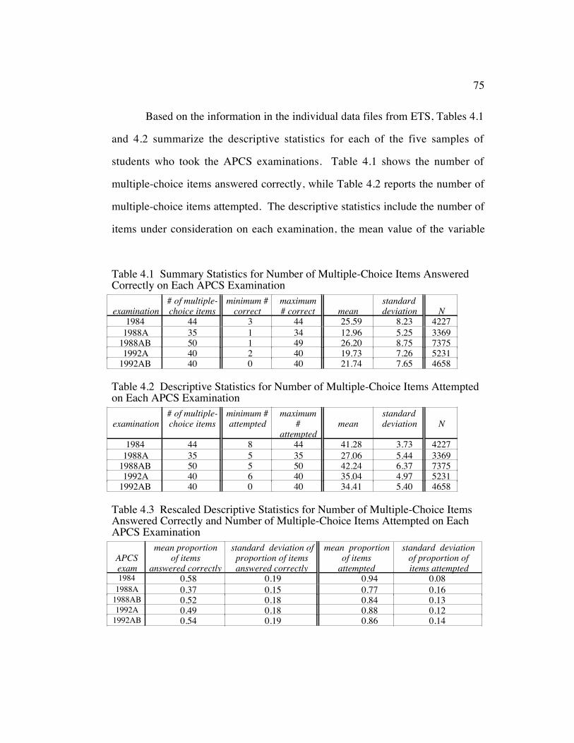
75

Based on the information in the individual data files from ETS, Tables 4.1

and 4.2 summarize the descriptive statistics for each of the five samples of

students who took the APCS examinations. Table 4.1 shows the number of

multiple-choice items answered correctly, while Table 4.2 reports the number of

multiple-choice items attempted. The descriptive statistics include the number of

items under consideration on each examination, the mean value of the variable

Table 4.1 Summary Statistics for Number of Multiple-Choice Items AnsweredCorrectly on Each APCS Examination

examination# of multiple-choice items

minimum #correct

maximum# correct mean

standarddeviation N

1984 44 3 44 25.59 8.23 42271988A 35 1 34 12.96 5.25 3369

1988AB 50 1 49 26.20 8.75 73751992A 40 2 40 19.73 7.26 5231

1992AB 40 0 40 21.74 7.65 4658

Table 4.2 Descriptive Statistics for Number of Multiple-Choice Items Attemptedon Each APCS Examination

examination# of multiple-choice items

minimum #attempted

maximum#

attemptedmean

standarddeviation N

1984 44 8 44 41.28 3.73 42271988A 35 5 35 27.06 5.44 3369

1988AB 50 5 50 42.24 6.37 73751992A 40 6 40 35.04 4.97 5231

1992AB 40 0 40 34.41 5.40 4658

Table 4.3 Rescaled Descriptive Statistics for Number of Multiple-Choice ItemsAnswered Correctly and Number of Multiple-Choice Items Attempted on EachAPCS Examination

APCSexam

mean proportionof items

answered correctly

standard deviation ofproportion of itemsanswered correctly

mean proportionof items

attempted

standard deviationof proportion ofitems attempted

1984 0.58 0.19 0.94 0.081988A 0.37 0.15 0.77 0.16

1988AB 0.52 0.18 0.84 0.131992A 0.49 0.18 0.88 0.12

1992AB 0.54 0.19 0.86 0.14

76

(i.e., either number correct or number attempted) across all respondents, the

standard deviation, the range (minimum and maximum values), and the number of

respondents in the sample. Table 4.3 presents the means and standard deviations

from Tables 4.1 and 4.2 rescaled to the range [0.0,"0.1].

Two different views of performance can be developed from this

information: (1) the proportion of respondents from the total sample who

answered each item correctly and (2) the proportion of respondents who answered

each item correctly among those who attempted the item. Each view has certain

advantages; the research reported here used the first figure. This choice was made

for two reasons: (a) analyses for a particular examination were based on a

constant sample size across all items from that examination and (b) the fact that

an item was not attempted provided information about the perceived difficulty of

the item. In contrast, ETS used the second view of performance, the proportion of

respondents who answered the item correctly among those who attempted the

item. Because ETS assesses a “guessing penalty” on the multiple-choice section,

many students undoubtedly skipped items about which they were unsure in order

to avoid losing points. In addition, since each section of the examination was

given during a fixed period of time, some students may have run out of time

before completing all items on a section. Thus, students who worked more slowly

may not have had sufficient time to answer some items even though in other

circumstances they could have answered correctly. The second view takes this

time constraint into consideration.

77

4.2 CONTENT ANALYSIS PROCEDURE RESULTS

The outcome of the final phase of the content analysis procedure is

reported in this section. A pilot phase was also run; these results will be discussed

as appropriate.

4.2.1 The instruments under study

The final content analysis procedure considered four distinct examination

packets: 1984, 1988, 1992A, and 1992B. Although the 1988 examination was

administered in two versions to two different samples of students, the multiple-

choice section of version A of the 1988 examination was a subset of the items

from version AB (i.e., 35 of 50 items appeared on both the A and AB versions).

As a result, the content analysis procedure considered only the AB examination

packet for 1988. On the 1992 examination, 15 items on the A and AB versions

were identical; the packets were not modified to remove this redundancy.

The four examination packets included a total of 174 multiple-choice

items. Eliminating the second occurrence of the 15 duplicate items from the 1992

examination (i.e., counting each one only once) resulted in a total of 159 distinct

multiple-choice items that were considered in the final phase. The pilot phase of

the content analysis procedure used only the 1984 and 1988 APCS examinations,

for a total of 94 multiple-choice items.

4.2.2 The judges

The final content analysis procedure was completed by 38 computer

science educators during the period from June through November, 1993. Two of

the judges did not rate the items from the 1988 examination, so the number of

78

judges for the 1988 APCS examination was 36. Of these judges at the time of the

content analysis:

• 10 were high school teachers

• 25 were instructors at a college or university

• 6 had completed the rating task during both the pilot and final phases

• 21 had served as readers in grading the 1992 APCS free-response items

• 11 had participated in an NSF-sponsored workshop on the use of formal

methods in the undergraduate curriculum during summer 1993

• several had written introductory textbooks on various subjects in the field

of computer science

• two had been recognized as “Outstanding Educator of the Year” by the

Association for Computing Machinery’s Special Interest Group on

Computer Science Education (ACM SIGCSE)

• one had received the Turing Award, the highest honor available in the

computing field (considered analogous in prestige to the Nobel Awards)

4.2.3 Partitioning the items during the final phase

A key goal of this study was to contrast performance on items judged to

have a strong relationship to the subdomain of logic with performance on items

that were judged to have little or no relationship to logic. During the final phase

of the procedure, each judge rated each item with one of four categories that

indicated the perceived strength-of-relationship between the concepts covered by

the item and the concepts of logic. The categories were ‘main concept’, ‘vital

subconcept’, ‘trivial subconcept’, and ‘not used’. A rating of ‘main concept’ or

79

‘vital subconcept’ for an item indicated that the judge perceived logic to be an

important aspect of that item; a high occurrence of these two categories caused

the item to be assigned to the strongly related partition. Similarly, ‘trivial

subconcept’ and ‘not used’ indicated a perceived unimportance of the concepts of

logic in the context of the item; a high occurrence of these two categories caused

the item to be assigned to the not strongly related partition.

Two different algorithms were used in creating the partitions of items.

The liberal partitioning algorithm classified an item as strongly related if at least

50% of the judges had rated the item ‘main concept’ or ‘vital subconcept’ and as

not strongly related otherwise. Under the liberal partitioning algorithm, all items

fell into one of the two partitions. The conservative partitioning algorithm used

stricter criteria for assigning items to partitions, with the result that a number of

items were excluded from consideration during further analysis. In the

conservative algorithm, an item was classified as strongly related if 75% or more

of the judges had rated the item ‘main concept’ or ‘vital subconcept’. In order to

be put in the not strongly related partition under the conservative algorithm, at

least 75% of the judges must have rated the item as ‘trivial subconcept’ or ‘not

used’. Table 4.4 summarizes the number of items in each partition under the two

partitioning algorithms for each of the five examination versions. Appendix F

presents the detailed results from the content analysis judging, including the

number of judges who chose specific categories for each item and the assignment

of individual items to partitions under both the liberal and conservative

partitioning algorithms.

80

Sample APCS examination items are given in Figures 4.1 through 4.4.

Figures 4.1 and 4.2 show items that 37 out of 38 judges (97%) rated as either

‘main concept’ or ‘vital subconcept’; these items were assigned to the strongly

related partition under both the liberal and the conservative partitioning

algorithms. Figure 4.3 shows an item that 74% of the judges rated as either ‘main

concept’ or ‘vital subconcept’; this item was assigned to the strongly related

partition under the liberal partitioning algorithm but was eliminated from

consideration under the conservative partitioning algorithm. Figure 4.4 shows an

item that only one out of 38 of the judges (3%) rated as either ‘main concept’ or

‘vital subconcept’; this item was assigned to the not strongly related partition

under both the liberal and the conservative partitioning algorithms. Appendix G

presents the 22 multiple-choice items that were classified as strongly related

under the conservative partitioning algorithm.

Table 4.4 Summary of Number of Items in Each Partition under EachPartitioning Algorithm for Each APCS Examination

APCS liberal partitioning algorithm conservative partitioning algorithm examinationand version

stronglyrelated

not stronglyrelated

total # ofitems

stronglyrelated

not stronglyrelated

total # ofitems

1984 10 34 44 4 30 341988A 11 24 35 4 17 21

1988AB 14 36 50 5 29 341992A 16 24 40 8 13 21

1992AB 14 26 40 9 18 27

Note: The A version of the 1988 examination consists of the first 35 multiple-choice itemsfrom the AB version of the 1988 examination.

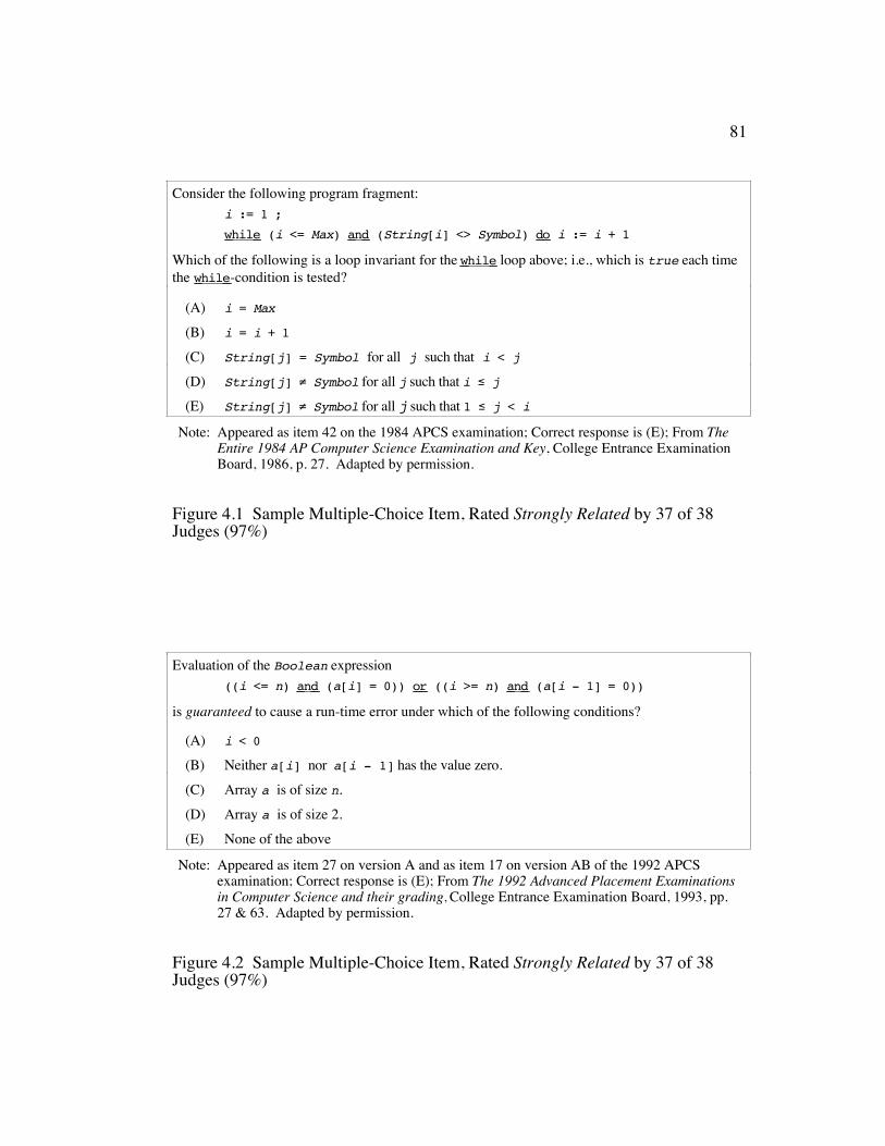
81

Consider the following program fragment:i := 1 ; while (i <= Max) and (String[i] <> Symbol) do i := i + 1

Which of the following is a loop invariant for the while loop above; i.e., which is true each timethe while -condition is tested?

(A) i = Max

(B) i = i + 1

(C) String[j] = Symbol for all j such that i < j(D) String[j] ≠ Symbol for all j such that i ≤ j(E) String[j] ≠ Symbol for all j such that 1 ≤ j < i

Note: Appeared as item 42 on the 1984 APCS examination; Correct response is (E); From TheEntire 1984 AP Computer Science Examination and Key, College Entrance ExaminationBoard, 1986, p. 27. Adapted by permission.

Figure 4.1 Sample Multiple-Choice Item, Rated Strongly Related by 37 of 38Judges (97%)

Evaluation of the Boolean expression((i <= n) and (a[i] = 0)) or ((i >= n) and (a[i - 1] = 0))

is guaranteed to cause a run-time error under which of the following conditions?

(A) i < 0

(B) Neither a[i] nor a[i - 1] has the value zero.(C) Array a is of size n.(D) Array a is of size 2.(E) None of the above

Note: Appeared as item 27 on version A and as item 17 on version AB of the 1992 APCSexamination; Correct response is (E); From The 1992 Advanced Placement Examinationsin Computer Science and their grading, College Entrance Examination Board, 1993, pp.27 & 63. Adapted by permission.

Figure 4.2 Sample Multiple-Choice Item, Rated Strongly Related by 37 of 38Judges (97%)

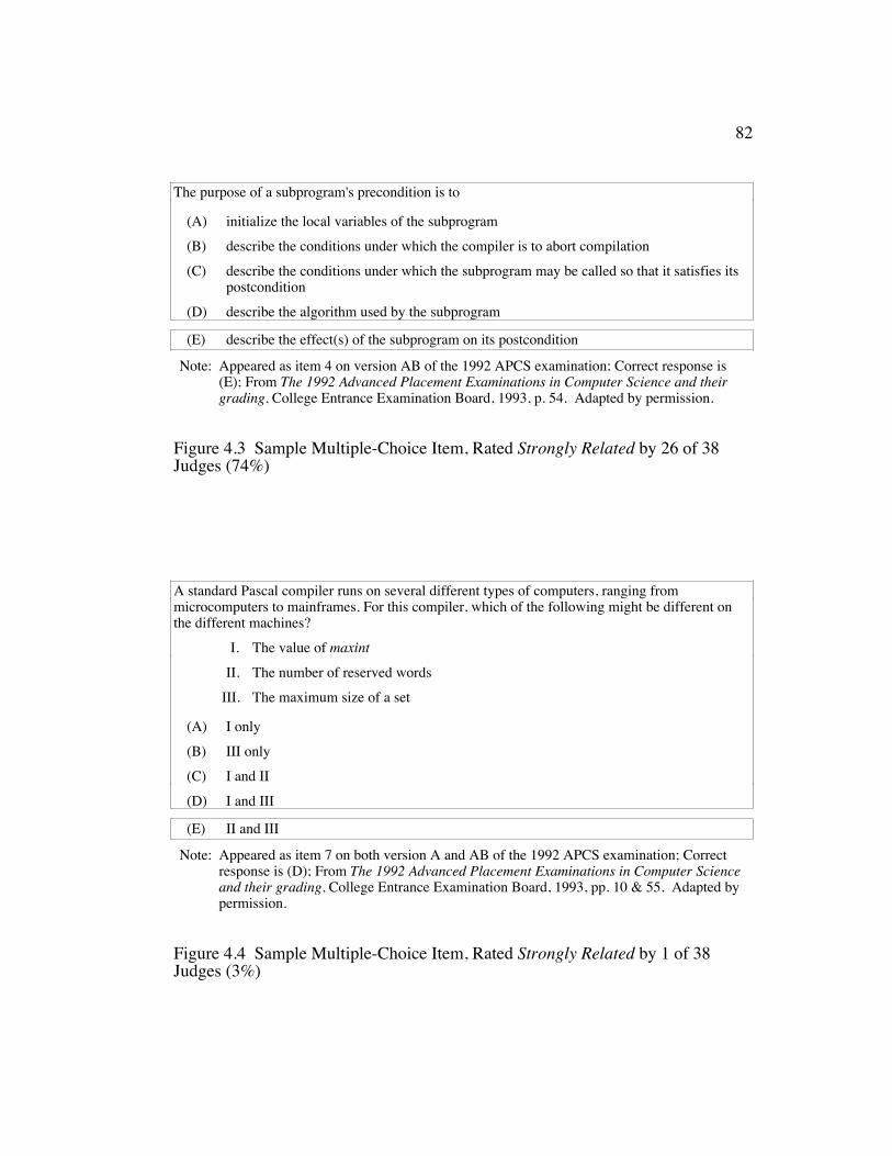
82

The purpose of a subprogram's precondition is to

(A) initialize the local variables of the subprogram(B) describe the conditions under which the compiler is to abort compilation(C) describe the conditions under which the subprogram may be called so that it satisfies its

postcondition(D) describe the algorithm used by the subprogram

(E) describe the effect(s) of the subprogram on its postcondition

Note: Appeared as item 4 on version AB of the 1992 APCS examination; Correct response is(E); From The 1992 Advanced Placement Examinations in Computer Science and theirgrading, College Entrance Examination Board, 1993, p. 54. Adapted by permission.

Figure 4.3 Sample Multiple-Choice Item, Rated Strongly Related by 26 of 38Judges (74%)

A standard Pascal compiler runs on several different types of computers, ranging frommicrocomputers to mainframes. For this compiler, which of the following might be different onthe different machines?

I. The value of maxintII. The number of reserved words

III. The maximum size of a set

(A) I only(B) III only(C) I and II(D) I and III

(E) II and III

Note: Appeared as item 7 on both version A and AB of the 1992 APCS examination; Correctresponse is (D); From The 1992 Advanced Placement Examinations in Computer Scienceand their grading, College Entrance Examination Board, 1993, pp. 10 & 55. Adapted bypermission.

Figure 4.4 Sample Multiple-Choice Item, Rated Strongly Related by 1 of 38Judges (3%)

83

4.2.4 Content analysis reliability results

The content analysis reliability procedures were run for each of the four

examination packets. For each packet, these calculations resulted in an overall

reliability value, a single category reliability value for each of the four

classification categories, and individual judge reliability.

4.2.4.1 Overall reliability

In producing the overall reliability figures two different models were

considered, the four-category model and the two-category model. In the four-

category model, the distinct classification categories were maintained, giving the

categories ‘main concept’, ‘vital subconcept’, ‘trivial subconcept’, and ‘not used’.

The two-category model was based on two collapsed categories: the

classification categories ‘main concept’ and ‘vital subconcept’ became the single

collapsed category strongly related, while the classification categories ‘trivial

subconcept and ‘not used’ became the single collapsed category not strongly

related.

The agreement coefficients for the overall reliability of the content

Table 4.5 Agreement Coefficients Showing Overall Reliability of the ContentAnalysis of the APCS Examinations

liberal partitioning algorithm conservative partitioning algorithm APCS

examinationwith all fourcategories

with collapsedcategories

with all fourcategories

with collapsedcategories

1984 0.325 0.458 0.290 0.4731988 A & AB 0.310 0.434 0.303 0.496

1992A 0.317 0.405 0.458 0.7041992AB 0.340 0.494 0.391 0.694

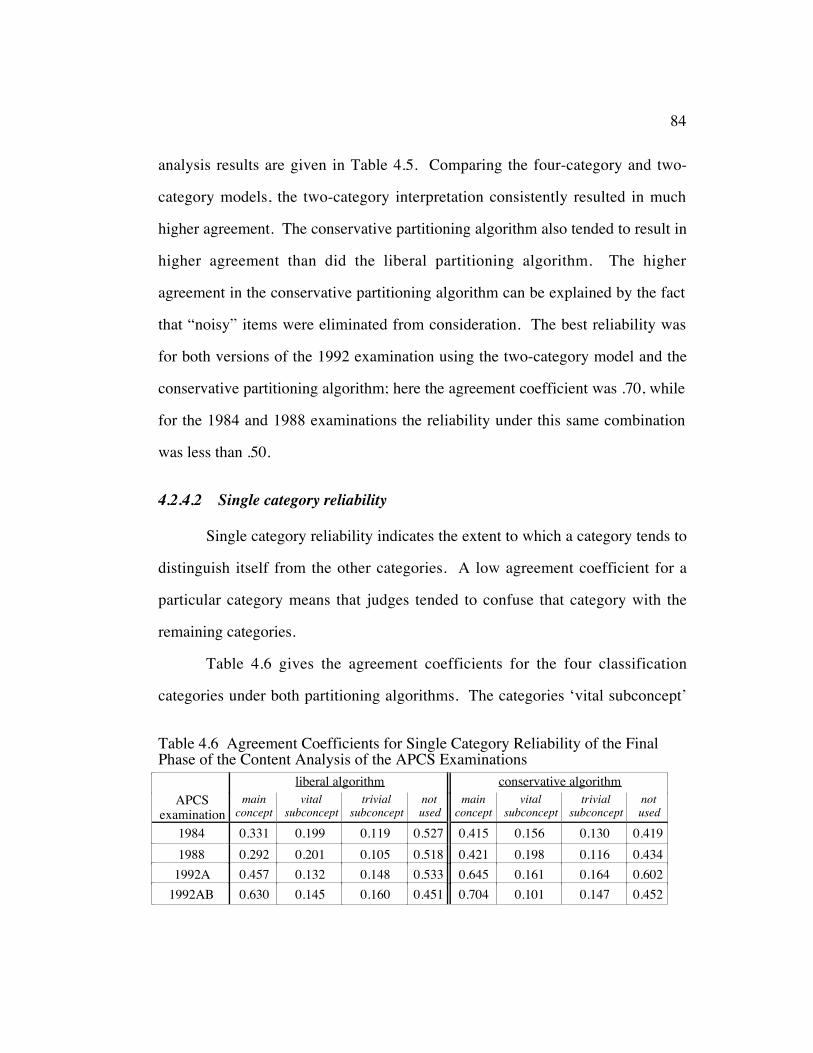
84

analysis results are given in Table 4.5. Comparing the four-category and two-

category models, the two-category interpretation consistently resulted in much

higher agreement. The conservative partitioning algorithm also tended to result in

higher agreement than did the liberal partitioning algorithm. The higher

agreement in the conservative partitioning algorithm can be explained by the fact

that “noisy” items were eliminated from consideration. The best reliability was

for both versions of the 1992 examination using the two-category model and the

conservative partitioning algorithm; here the agreement coefficient was .70, while

for the 1984 and 1988 examinations the reliability under this same combination

was less than .50.

4.2.4.2 Single category reliability

Single category reliability indicates the extent to which a category tends to

distinguish itself from the other categories. A low agreement coefficient for a

particular category means that judges tended to confuse that category with the

remaining categories.

Table 4.6 gives the agreement coefficients for the four classification

categories under both partitioning algorithms. The categories ‘vital subconcept’

Table 4.6 Agreement Coefficients for Single Category Reliability of the FinalPhase of the Content Analysis of the APCS Examinations

liberal algorithm conservative algorithm APCS

examinationmain

conceptvital

subconcepttrivial

subconceptnotused

mainconcept

vitalsubconcept

trivialsubconcept

notused

1984 0.331 0.199 0.119 0.527 0.415 0.156 0.130 0.4191988 0.292 0.201 0.105 0.518 0.421 0.198 0.116 0.434

1992A 0.457 0.132 0.148 0.533 0.645 0.161 0.164 0.6021992AB 0.630 0.145 0.160 0.451 0.704 0.101 0.147 0.452

85

and ‘trivial subconcept’ tended to be highly unreliable, with agreement

coefficients that were at most .20. The ‘not used’ category had the highest

reliability, with agreement coefficients ranging from .45 to .53 when considering

the partitions defined by the liberal algorithm (which included all items) and from

.42 to .60 when considering the partitions defined by the conservative algorithm

(which included a reduced set of items). The ‘main concept’ category was

relatively reliable, with a range of .29 to .63 for the agreement coefficient when

considering the partitions defined by the liberal algorithm and from .41 to .70

when considering the partitions defined by the conservative algorithm.

During the pilot phase, the classification system was composed of four

categories that were unordered: ‘direct relationship’, ‘vital subconcept’, ‘parallel

concept’, and ‘not related’. After the classification system was refined for use in

the final phase, the new set of categories were ordered along a scale that ranged

from ‘main concept’ as the most strongly related category, moving down the scale

to ‘vital subconcept’, then to ‘trivial subconcept’, and, at the bottom of the scale,

‘not used’. Krippendorff (1980, p. 151) maintained that single-category reliability

can only be applied to unordered categories. However, because the single-

category reliability results obtained here are fully interpretable, this restriction

seems unnecessary.

4.2.4.3 Individual judge reliability

Individual judge reliability indicates the extent to which an individual

judge was the source of unreliable data (Krippendorff, 1980). Differences among

judges can be explained by work style (e.g., organized, neat, hurried), in

86

understanding of the instructions, in consistency of understanding of the concepts

under consideration, and in the way the items themselves are perceived.

Judge reliability was calculated as the agreement between a particular

judge and the pooled set of all other judges. Appendix H presents an overview of

individual reliability results for the final phase of the content analysis procedure.

Generally, individual judge reliability was much higher under the conservative

partitioning algorithm than under liberal partitioning algorithm. This difference

was fairly insignificant for the 1984 examination, but was pronounced for the

1988 and 1992 examinations.

An important issue relates to “outliers”: should judges whose individual

reliability deviated greatly from that of the other judges have been eliminated

from further consideration? As Krippendorff (1980) points out, this practice

needs to be treated with caution:

[A] practice, assertedly aimed at bypassing problems ofunreliability, is to take averages or majority judgments as truevalues whenever disagreements among independent observers areencountered. Such data do contain evidence about reproducibilitybefore the “undesirable” variance is eliminated. But, sincedisagreement implies nothing about who is right and who is wrong,neither the mean nor the mode has the wisdom required to improvedata reliability by computational means. An even more deceptivepractice is to admit only those data to an investigation on whichindependent coders achieve perfect agreement. The bias here istwo-fold. The procedure does not prevent chance agreements fromentering the data … and it biases the data toward what is easilycodable. (p. 132)

However, Krippendorff does concede that, if a particular judge proves to be very

unreliable, the data contributed by that judge “could be removed, checked, or

recoded by the other … coders [and] data reliability would improve …” (p. 150).

The decision in this study was to retain all judges.

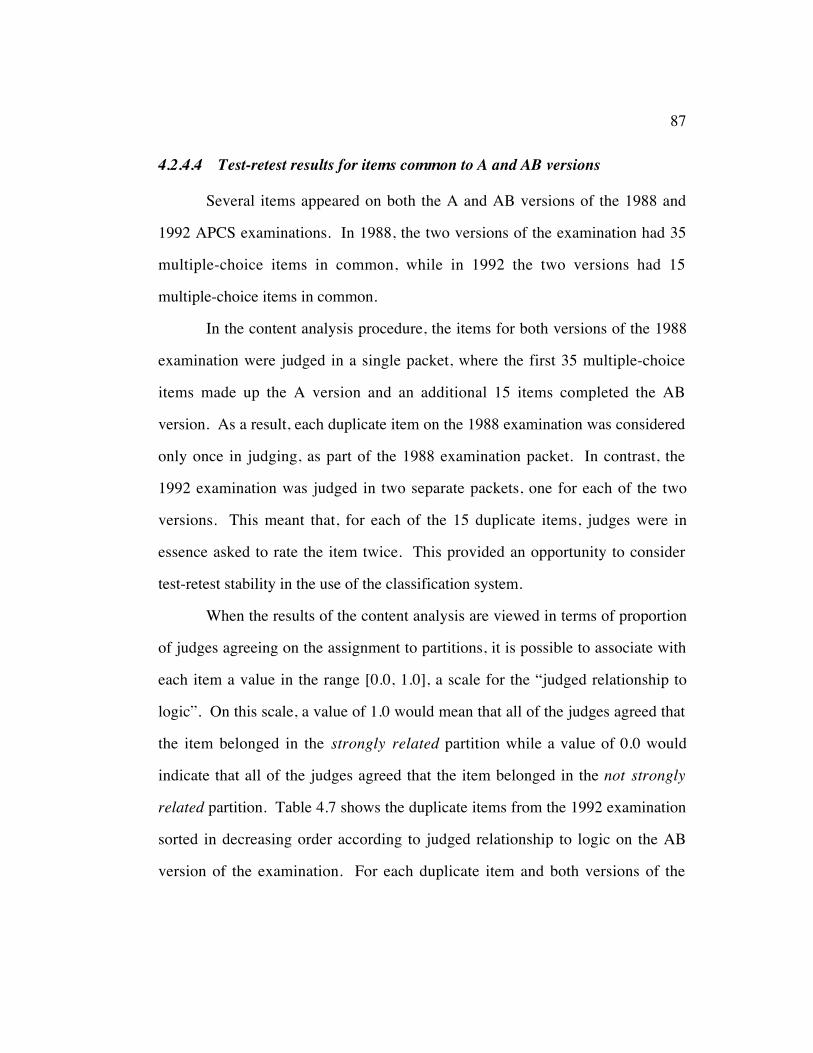
87

4.2.4.4 Test-retest results for items common to A and AB versions

Several items appeared on both the A and AB versions of the 1988 and

1992 APCS examinations. In 1988, the two versions of the examination had 35

multiple-choice items in common, while in 1992 the two versions had 15

multiple-choice items in common.

In the content analysis procedure, the items for both versions of the 1988

examination were judged in a single packet, where the first 35 multiple-choice

items made up the A version and an additional 15 items completed the AB

version. As a result, each duplicate item on the 1988 examination was considered

only once in judging, as part of the 1988 examination packet. In contrast, the

1992 examination was judged in two separate packets, one for each of the two

versions. This meant that, for each of the 15 duplicate items, judges were in

essence asked to rate the item twice. This provided an opportunity to consider

test-retest stability in the use of the classification system.

When the results of the content analysis are viewed in terms of proportion

of judges agreeing on the assignment to partitions, it is possible to associate with

each item a value in the range [0.0, 1.0], a scale for the “judged relationship to

logic”. On this scale, a value of 1.0 would mean that all of the judges agreed that

the item belonged in the strongly related partition while a value of 0.0 would

indicate that all of the judges agreed that the item belonged in the not strongly

related partition. Table 4.7 shows the duplicate items from the 1992 examination

sorted in decreasing order according to judged relationship to logic on the AB

version of the examination. For each duplicate item and both versions of the

88

examination, the agreement value and the associated item number is given. Based

on the criteria defined by the liberal and conservative partitioning algorithms,

each of these 15 items was assigned to the same partition for both versions of the

examination.

Differences in rating the same item on the two different versions could

indicate any of several phenomena, including problems with the classification

system, changes in the judges’ perceptions as they proceeded through the rating

task, and the influence that the order in which the examinations were considered

on classification results. Some judges reported that they recognized the item

Table 4.7 Comparison of Content Analysis Ratings on Duplicate Items from Aand AB Versions of the 1992 APCS Examination

itemjudged relationship

to logicfor A-version

judged relationshipto logic

for AB-version

item # on A-version of 1992

examination

item # on AB-version of 1992

examination1 1.00 1.00 1992A-32 1992B-212 1.00 1.00 1992A-26 1992B-163 0.97 0.97 1992A-27 1992B-174 1.00 0.95 1992A-31 1992B-185 0.74 0.68 1992A-08 1992B-046 0.74 0.68 1992A-20 1992B-067 0.42 0.34 1992A-29 1992B-298 0.42 0.32 1992A-10 1992B-109 0.39 0.32 1992A-09 1992B-0910 0.29 0.29 1992A-05 1992B-0511 0.03 0.03 1992A-07 1992B-0712 0.08 0.11 1992A-02 1992B-0213 0.08 0.08 1992A-28 1992B-2814 0.05 0.05 1992A-37 1992B-3715 0.05 0.05 1992A-38 1992B-38

Note: Items are sorted according to “judged relationship to logic” on AB version; on this scale,1.0 means all judges agreed the item belonged in the strongly related partition; 0.0 meansthat all judges agreed the item belonged in the not strongly related partition

89

repetition and attempted to achieve consistency between versions. For a fully

accurate indication of consistency in using the classification system, a judge

would have to had to rate each duplicate item on the two versions of the

examination without cross-referencing. Because, by their own admission, several

judges did do cross-referencing as they noticed duplicate items, the consistency

figures are inflated. However, even with cross-checking, none of the 38 judges

succeeded in rating all 15 items consistently. This shows that various factors

must have influenced the choice of categories from one packet to the other.

Appendix I profiles details of the ratings, both in terms of how consistently each

judge rated the 15 items and in terms of how consistently each of the 15 items

were rated by the 38 judges.

4.3 RESEARCH QUESTIONS AND HYPOTHESIS TESTING

Based on the rating results from the content analysis procedure and the

data from ETS, the answers to the research questions posed at the end of

Chapter"1 can now be considered.

4.3.1 Descriptive statistics for performance differential between partitions

The research question that drove the design of the methodology used in

this study was:

(a) Can a procedure be developed for reliable and valid classification of

content-area test items according to their degree of relationship to a pre-

defined set of logic concepts?

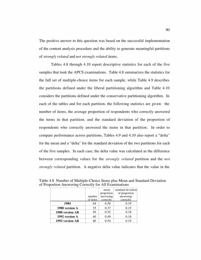
90

The positive answer to this question was based on the successful implementation

of the content analysis procedure and the ability to generate meaningful partitions

of strongly related and not strongly related items.

Tables 4.8 through 4.10 report descriptive statistics for each of the five

samples that took the APCS examinations. Table 4.8 summarizes the statistics for

the full set of multiple-choice items for each sample, while Table 4.9 describes

the partitions defined under the liberal partitioning algorithm and Table 4.10

considers the partitions defined under the conservative partitioning algorithm. In

each of the tables and for each partition, the following statistics are given: the

number of items, the average proportion of respondents who correctly answered

the items in that partition, and the standard deviation of the proportion of

respondents who correctly answered the items in that partition. In order to

compare performance across partitions, Tables 4.9 and 4.10 also report a “delta”

for the mean and a “delta” for the standard deviation of the two partitions for each

of the five samples. In each case, the delta value was calculated as the difference

between corresponding values for the strongly related partition and the not

strongly related partition. A negative delta value indicates that the value in the

Table 4.8 Number of Multiple-Choice Items plus Mean and Standard Deviationof Proportion Answering Correctly for All Examinations

numberof items

meanproportionansweringcorrectly

standard deviationof proportion

answeringcorrectly

1984 44 0.58 0.191988 version A 35 0.37 0.15

1988 version AB 50 0.52 0.181992 version A 40 0.49 0.18

1992 version AB 40 0.54 0.19

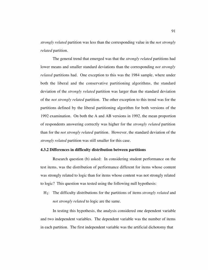
91

strongly related partition was less than the corresponding value in the not strongly

related partition.

The general trend that emerged was that the strongly related partitions had

lower means and smaller standard deviations than the corresponding not strongly

related partitions had. One exception to this was the 1984 sample, where under

both the liberal and the conservative partitioning algorithms, the standard

deviation of the strongly related partition was larger than the standard deviation

of the not strongly related partition. The other exception to this trend was for the

partitions defined by the liberal partitioning algorithm for both versions of the

1992 examination. On both the A and AB versions in 1992, the mean proportion

of respondents answering correctly was higher for the strongly related partition

than for the not strongly related partition. However, the standard deviation of the

strongly related partition was still smaller for this case.

4.3.2 Differences in difficulty distribution between partitions

Research question (b) asked: In considering student performance on the

test items, was the distribution of performance different for items whose content

was strongly related to logic than for items whose content was not strongly related

to logic? This question was tested using the following null hypothesis:

H1: The difficulty distributions for the partitions of items strongly related and

not strongly related to logic are the same.

In testing this hypothesis, the analysis considered one dependent variable

and two independent variables. The dependent variable was the number of items

in each partition. The first independent variable was the artificial dichotomy that

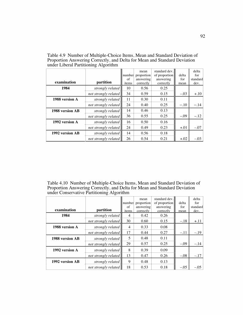
92

Table 4.9 Number of Multiple-Choice Items, Mean and Standard Deviation ofProportion Answering Correctly, and Delta for Mean and Standard Deviationunder Liberal Partitioning Algorithm

examination partition

numberof

items

meanproportionansweringcorrectly

standard dev.of proportion

answeringcorrectly

deltafor

mean

deltafor

standarddev.

1984 strongly related 10 0.56 0.25not strongly related 34 0.59 0.15 –.03 +.10

1988 version A strongly related 11 0.30 0.11not strongly related 24 0.40 0.25 –.10 –.14

1988 version AB strongly related 14 0.46 0.13not strongly related 36 0.55 0.25 –.09 –.12

1992 version A strongly related 16 0.50 0.16not strongly related 24 0.49 0.23 +.01 –.07

1992 version AB strongly related 14 0.56 0.18not strongly related 26 0.54 0.21 +.02 –.03

Table 4.10 Number of Multiple-Choice Items, Mean and Standard Deviation ofProportion Answering Correctly, and Delta for Mean and Standard Deviationunder Conservative Partitioning Algorithm

examination partition

numberof

items

meanproportionansweringcorrectly

standard dev.of proportion

answeringcorrectly

deltafor

mean

deltafor

standarddev.

1984 strongly related 4 0.42 0.26not strongly related 30 0.60 0.15 –.18 +.11

1988 version A strongly related 4 0.33 0.08not strongly related 17 0.44 0.27 –.11 –.19

1988 version AB strongly related 5 0.48 0.11not strongly related 29 0.57 0.25 –.09 –.14

1992 version A strongly related 8 0.39 0.09not strongly related 13 0.47 0.26 –.08 –.17

1992 version AB strongly related 9 0.48 0.13not strongly related 18 0.53 0.18 –.05 –.05

93

divided the items into the strongly related and not strongly related partitions. The

second independent variable stratified the items according to difficulty. The

operational definition for difficulty of an item depended on the proportion of

students who correctly answered the item. The categories of difficulty, which

were mutually exclusive, were defined in terms of the proportion of respondents

who answered correctly: ‘very difficult’ for the interval [.0, .2), ‘somewhat

difficult’ for the interval [.2, .4), ‘average’ for the interval [.4, .6) ‘somewhat

easy’ for the interval [.6, .8), and ‘very easy’ for the interval [.8, 1.0].

Because the number of items in some categories was so small, the results

from the five examinations were pooled for this analysis. Table 4.11 presents the

number of items at each level of difficulty in each partition under the liberal

partitioning algorithm. Figure 4.5 presents the same data in the form of a graph,

where the x-axis is the difficulty category and the y-axis is the proportion of items

that fell into a partition; the difficulty distribution for each partition is plotted as a

line. Table 4.12 and Figure 4.6 present the same information for the partitions

defined by the conservative partitioning algorithm.

To test whether the strongly related and not strongly related partitions

were homogeneous with respect to the five levels of item difficulty, hierarchical

log-linear tests of homogeneity were run on the data in Tables 4.11 and 4.12. An

important consideration in using this test was the number of cells in the 5X2 table

for which there was no item. When this occurs, the empty cells are accidents of

the sampling procedure, known as random zeroes. When random zeroes are

sufficiently prevalent, they can prevent completion of the log-linear test of fit

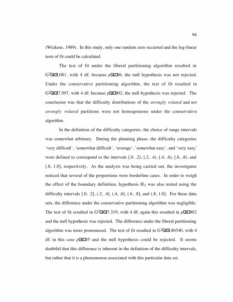
94

(Wickens, 1989). In this study, only one random zero occurred and the log-linear

tests of fit could be calculated.

The test of fit under the liberal partitioning algorithm resulted in

G2"="9.081, with 4 df; because p"=".06, the null hypothesis was not rejected.

Under the conservative partitioning algorithm, the test of fit resulted in

G2"="17.507, with 4 df; because p"≤".002, the null hypothesis was rejected. The

conclusion was that the difficulty distributions of the strongly related and not

strongly related partitions were not homogeneous under the conservative

algorithm.

In the definition of the difficulty categories, the choice of range intervals

was somewhat arbitrary. During the planning phase, the difficulty categories

‘very difficult’, ‘somewhat difficult’, ‘average’, ‘somewhat easy’, and ‘very easy’

were defined to correspond to the intervals [.0, .2), [.2, .4), [.4, .6), [.6, .8), and

[.8, 1.0], respectively. As the analysis was being carried out, the investigator

noticed that several of the proportions were borderline cases. In order to weigh

the effect of the boundary definition, hypothesis H1 was also tested using the

difficulty intervals [.0, .2], (.2, .4], (.4, .6], (.6, .8], and (.8, 1.0]. For these data

sets, the difference under the conservative partitioning algorithm was negligible:

The test of fit resulted in G2"="17.319, with 4 df; again this resulted in p"≤".002

and the null hypothesis was rejected. The difference under the liberal partitioning

algorithm was more pronounced. The test of fit resulted in G2"="9.86540, with 4

df; in this case p"≤".05 and the null hypothesis could be rejected. It seems

doubtful that this difference is inherent in the definition of the difficulty intervals,

but rather that it is a phenomenon associated with this particular data set.

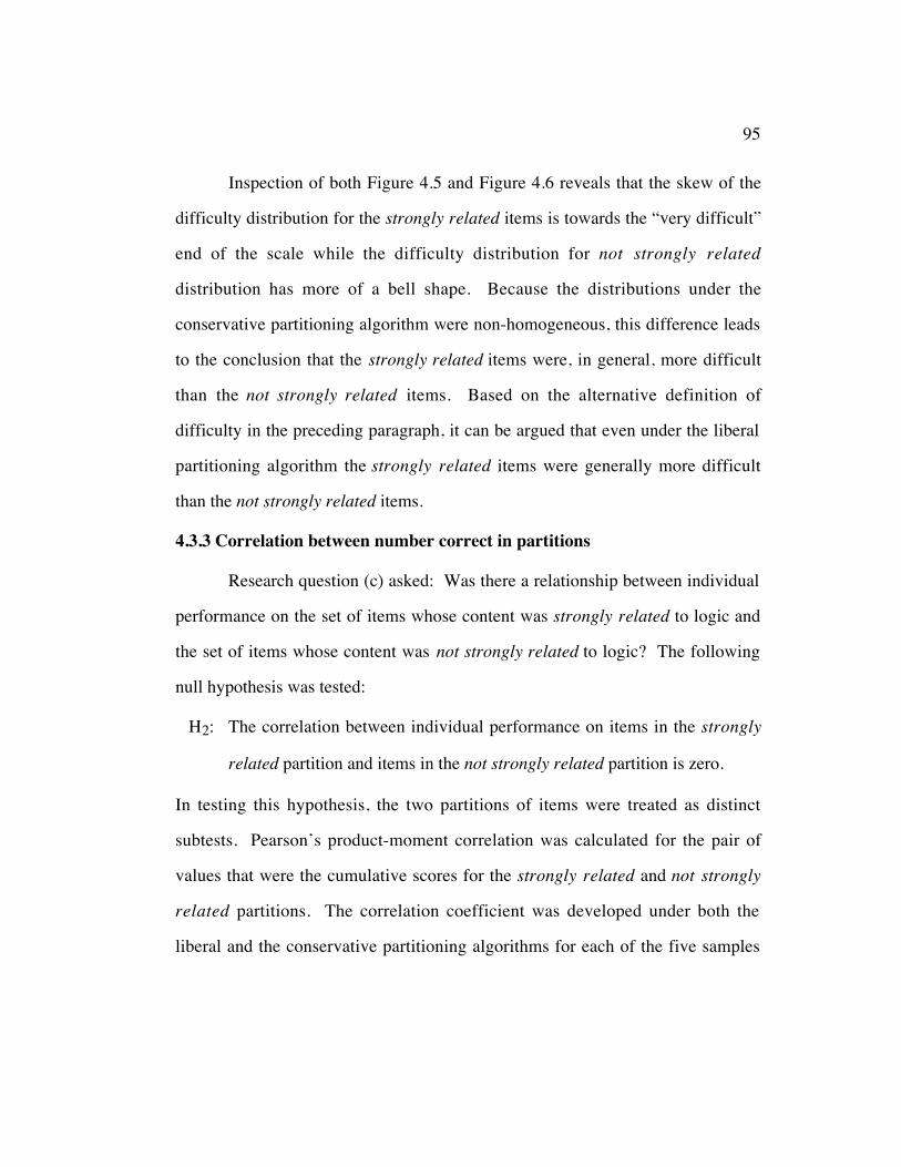
95

Inspection of both Figure 4.5 and Figure 4.6 reveals that the skew of the

difficulty distribution for the strongly related items is towards the “very difficult”

end of the scale while the difficulty distribution for not strongly related

distribution has more of a bell shape. Because the distributions under the

conservative partitioning algorithm were non-homogeneous, this difference leads

to the conclusion that the strongly related items were, in general, more difficult

than the not strongly related items. Based on the alternative definition of

difficulty in the preceding paragraph, it can be argued that even under the liberal

partitioning algorithm the strongly related items were generally more difficult

than the not strongly related items.

4.3.3 Correlation between number correct in partitions

Research question (c) asked: Was there a relationship between individual

performance on the set of items whose content was strongly related to logic and

the set of items whose content was not strongly related to logic? The following

null hypothesis was tested:

H2: The correlation between individual performance on items in the strongly

related partition and items in the not strongly related partition is zero.

In testing this hypothesis, the two partitions of items were treated as distinct

subtests. Pearson’s product-moment correlation was calculated for the pair of

values that were the cumulative scores for the strongly related and not strongly

related partitions. The correlation coefficient was developed under both the

liberal and the conservative partitioning algorithms for each of the five samples

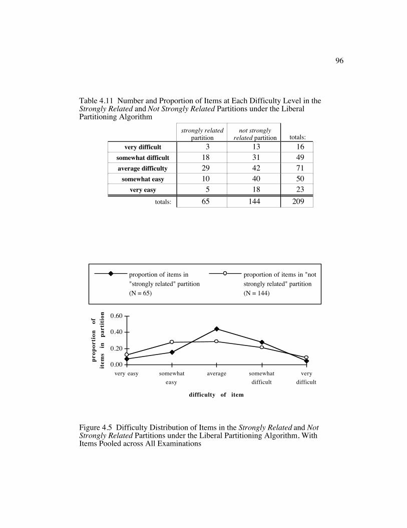
96

Table 4.11 Number and Proportion of Items at Each Difficulty Level in theStrongly Related and Not Strongly Related Partitions under the LiberalPartitioning Algorithm

strongly relatedpartition

not stronglyrelated partition totals:

very difficult 3 13 16somewhat difficult 18 31 49average difficulty 29 42 71

somewhat easy 10 40 50very easy 5 18 23

totals: 65 144 209

difficulty of item

prop

orti

on

ofit

ems

in

part

itio

n

0.00

0.20

0.40

0.60

very easy somewhateasy

average somewhatdifficult

verydifficult

proportion of items in"strongly related" partition(N = 65)

proportion of items in "notstrongly related" partition(N = 144)

Figure 4.5 Difficulty Distribution of Items in the Strongly Related and NotStrongly Related Partitions under the Liberal Partitioning Algorithm, WithItems Pooled across All Examinations

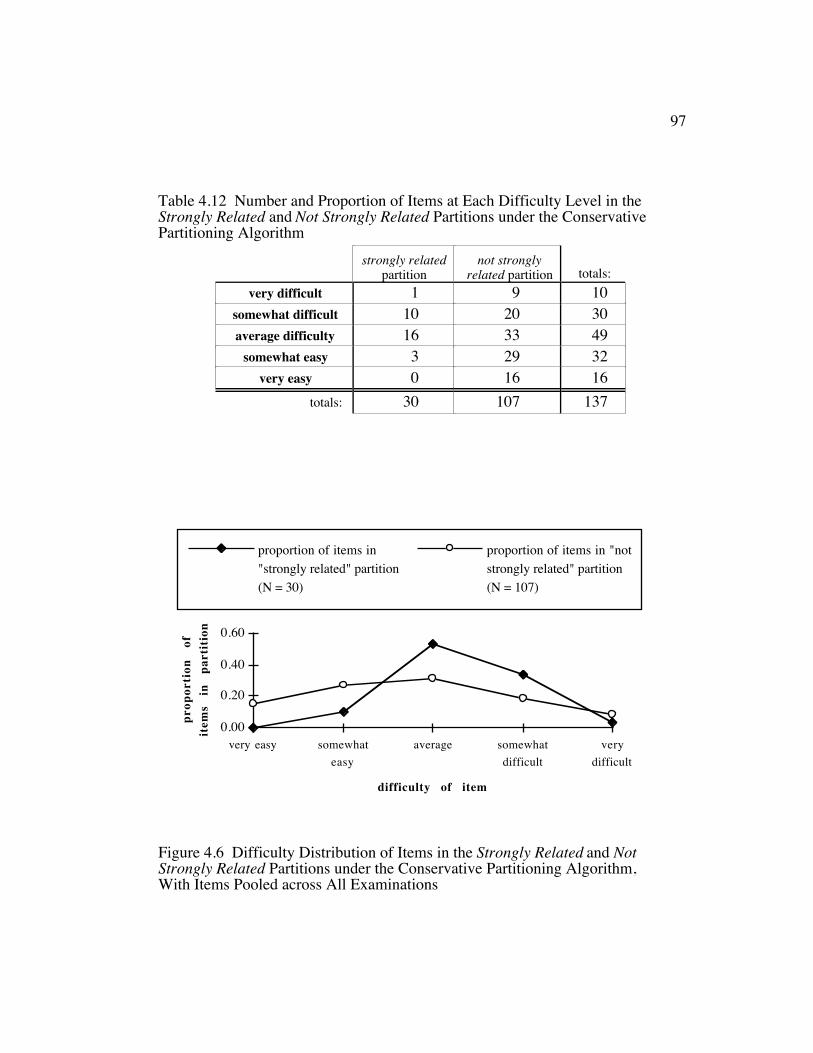
97

Table 4.12 Number and Proportion of Items at Each Difficulty Level in theStrongly Related and Not Strongly Related Partitions under the ConservativePartitioning Algorithm

strongly relatedpartition

not stronglyrelated partition totals:

very difficult 1 9 10somewhat difficult 10 20 30average difficulty 16 33 49

somewhat easy 3 29 32very easy 0 16 16

totals: 30 107 137

difficulty of item

prop

orti

on

ofit

ems

in

part

itio

n

0.00

0.20

0.40

0.60

very easy somewhateasy

average somewhatdifficult

verydifficult

proportion of items in"strongly related" partition(N = 30)

proportion of items in "notstrongly related" partition(N = 107)

Figure 4.6 Difficulty Distribution of Items in the Strongly Related and NotStrongly Related Partitions under the Conservative Partitioning Algorithm,With Items Pooled across All Examinations

98

(1984, 1988 version A, 1988 version AB, 1992 version A, and 1992 version AB).

In addition, the coefficient of determination was calculated from each correlation

coefficient; this value is the square of the correlation coefficient and is used to

describe the shared variance in the two-score distribution.

Table 4.13 reports the correlation coefficients and coefficients of

determination for the five samples. Several factors influence the value of the

correlation coefficient; these will be considered in the context of this study. First,

as the number of items per subtest increases the possible variation of the scores

increases and, in turn, the correlations tend to be higher. Here, the subtests

defined under the liberal partitioning algorithm had more items than the

analogous subtests under the conservative algorithm; the correlations under the

liberal partitioning algorithm were consistently larger than the correlations under

the conservative partitioning algorithm. Second, as samples become more

homogeneous, the possible variation in scores becomes smaller; as a result,

correlations tend to be lower for homogeneous samples. In this study, the only

instance where a sample was reported to be more homogeneous was for version

AB of the 1992 examination. This increased homogeneity was because two

distinct examinations were given in 1992 rather than a two-section AB version as

in 1988 or a single examination as in 1984 (R. Morgan, personal communication,

April 14, 1994). In spite of the increased homogeneity, the correlation

coefficients for the sample that took version AB of the 1992 examination were

among the highest under both partitioning algorithms.

99

A factor that could have influenced the value of the correlation coefficient

was the effect of removing items from consideration under the conservative

partitioning algorithm. In a sense, the eliminated items had something in common

with one another, perhaps to the extent that they were measuring some of the

same abilities. This reasoning leads to the conclusion that the higher correlations

between the partitions defined by the liberal partitioning algorithm could have

been due in part to the inclusion of the “mid-range” items (i.e., those items for

which only 25% to 75% of the judges agreed about the relationship).

As sample size increases, the correlation coefficient becomes more

reliable. In fact, for very large N, very small correlation coefficients can be

statistically significant. In this study, the sample sizes were very large, ranging

from 3,369 to 7,375. As expected, all correlation coefficients were significant at

p"≤".01. These results lead to the conclusion that null hypothesis H2 should be

rejected in all cases. Thus, there is a relationship between performance on items

in the strongly related partition and performance on items in the not strongly

related partition under both partitioning algorithms.

The shared variance between the strongly related and not strongly related

Table 4.13 Correlation between Number Correct in the Strongly Related and NotStrongly Related Partitions under Both Partitioning Algorithms

liberal partitioning algorithm conservative partitioning algorithm APCS

examinationcorrelationcoefficient

coefficient ofdetermination

correlationcoefficient

coefficient ofdetermination

1984 .74 .55 .60 .361988A .60 .36 .42 .18

1988AB .75 .56 .60 .361992A .74 .55 .56 .31

1992AB .75 .56 .64 .41

100

subtests, indicated by the coefficients of determination, was over 50% under the

liberal algorithm for the samples taking the 1984 examination, the AB version of

the 1988 examination, and both versions of the 1992 examination. Under the

liberal partitioning algorithm for the 1988 examination, only 36% of the variance

was shared by the two subtests. Under the conservative partitioning algorithm,

the shared variance was highest for version AB of the 1992 examination, at 41%.

For version A of the 1988 examination, only 18% of the variance was shared.

Under the conservative algorithm in all cases, less than 50% of the variability in

performance was shared variance. This suggests that to some extent different

cognitive abilities are required to answer correctly the items in the two partitions

defined under the conservative algorithm. This argues that the model that results

from the conservative partitioning algorithm is more descriptive than the model

defined under the liberal partitioning algorithm.

4.4 SUMMARY OF FINDINGS

In this section, the research questions are restated and the findings

summarized.

4.4.1 Development of the content analysis procedure

The first research question that was posed in Chapter 1 was:

(a) Can a procedure be developed for reliable and valid classification of

content-area test items according to their degree of relationship to a pre-

defined set of concepts?

This question addressed the feasibility of the methodology proposed for this

study. In Chapter 3 it was pointed out that, due to the nature of this question, no

101

null hypothesis would be formulated. Instead, the answer to the question was

based on the results of carrying out the content analysis described in Chapter 3.

Because the content analysis procedure was successfully developed and produced

acceptable results, the remaining research questions posed in Chapter 1 could be

considered.

4.4.2 Comparisons of partitions

In order to consider differences in performance across the partitions of

items defined in the content analysis procedure, the following research questions

were posed:

(b) In considering student performance on the test items, was the distribution

of performance different for items whose content was strongly related to

logic than for items whose content was not strongly related to logic?

(c) Was there a relationship between the pattern of responses on the set of

items whose content was strongly related to logic and the pattern of

responses on the set of items whose content was not strongly related to

logic?

Both of these research questions were informed by development of simple

descriptive statistics (mean and standard deviation) of performance on each set of

items. These values showed that, in general, the strongly related partitions had

lower means and smaller standard deviations than the corresponding not strongly

related partition had.

Question (b) was tested using the following null hypothesis:

102

H1: The difficulty distributions for the partitions of items strongly related and

not strongly related to logic are the same.

The difficulty distributions defined by the two sets of items were graphed and

tested for differences using a log-linear test of homogeneity. The null hypothesis

was rejected under the conservative partitioning algorithm but not under the

liberal partitioning algorithm. The conclusion was that the conservative

partitioning algorithm is the superior model for use in future studies.

Research question (c) was addressed by considering the null hypothesis:

H2: The correlation between individual performance on items in the strongly

related partition and items in the not strongly related partition is zero.

To test this hypothesis, the correlation coefficients for each pairing of item

partitions were generated (i.e. under both the liberal and the conservative

partitioning algorithms). The null hypothesis was rejected in all cases; however,

the practical significance of these results was negligible. The coefficient of

determination showed that, under the conservative partitioning algorithm, less

than 50% of the variance in performance on the two partitions was shared. Under

the liberal partitioning algorithm, this was true in only one case. Hence, the

conservative partitioning algorithm appears to provide a more descriptive model.

103

Chapter 5 Conclusions and Future Research

Chapter 5 discusses the conclusions that can be drawn about the research

questions based on the results of this study. The generalizability of the results is

considered. Finally, recommendations for future research are presented. The

dissertation closes with a brief epilogue that considers the instructional

implications of the results.

5.1 CONCLUSIONS REGARDING RESEARCH QUESTIONS

This research sought objective evidence as to whether novice computer

science students have more difficulty understanding concepts in the computer

science subdomain of mathematical logic than they generally have in

understanding other novice computer science concepts. This exploratory study

produced evidence that supported this conjecture.

The first research question that was posed in Chapter 1, developed in

Chapter 3, and explored in Chapter 4 was:

(a) Can a procedure be developed for reliable and valid classification of

content-area test items according to their degree of relationship to a pre-

defined set of logic concepts?

The content analysis procedure that emerged in the final phase of this study

provided a positive answer to this research question. The final procedure was

time-effective for the judges to complete, given that the item pool under

consideration was rather extensive. Reliability results showed that, in general, the

classification that emerged from the content analysis was consistent and reliable.

104

Content validity was established for the classification results, based on the

agreement of nearly 40 experts in computer science. The conclusion was that this

procedure resulted in the data needed to allow the study to continue. It is

recommended in the Future Research section that the content analysis procedure

developed for this study should be refined and applied in other research studies

both in the field of computer science and in other fields.

An unanticipated benefit was the insight this research provided into

differences in the way the multiple-choice items were perceived by the judges

who participated in this study. There was a great deal of variation among the

judges in their perceptions of which items included mathematical logic concepts

and to what degree. This observation underscores the lack of consensus within

the field of computing regarding the relationship between mathematical logic and

other computer science concepts. Suggestions for deeper exploration of this

phenomenon are discussed in the Future Research section.

While it would have been possible to train the judges to rate items more

consistently than they did in this study, such training was deemed undesirable.

An explicit decision was made to allow judges to use their expertise, bolstered by

the Quick Reference to Concepts in “Two-Valued Logic” in Figure 3.1, in doing

the classification. This freedom of interpretation and feedback from the judges

assisted the researcher in refining the taxonomy of concepts.

Given the results of the classification process during the final content

analysis procedure, the test items under consideration were divided into partitions

of items that were strongly related and not strongly related to logic. The

remaining research questions posed in Chapter 1 were the following:

105

(b) In considering student performance on the test items, was the distribution

of performance different on items whose content was strongly related to

logic than on items whose content was not strongly related to logic?

(c) Was there a relationship between individual performance on the set of

items whose content was strongly related to logic and the set of items

whose content was not strongly related to logic?

The answer to research question (b) was explored both through simple descriptive

statistics of student performance and by comparing the difficulty distributions of

the items in the strongly related and not strongly related partitions. In general,

the items in the strongly related partition were more difficult for the five samples

of students who took the APCS examinations that were considered in this

research. The answer to question (c) was investigated through the development of

correlation coefficients comparing individual performance on items in the two

partitions. The results of this analysis revealed systematic relationships between

the patterns of responses to items in the two partitions, suggesting that the

constructs being tested by items in each partition were related to one another. The

variability of individual responses to items in the strongly related partition

explained only a small amount of the variability of individual responses to items

in the not strongly related partition. Based on the amount of variance shared

between the two partitions, the conservative partitioning algorithm was more

discriminating than was the liberal partitioning algorithm.

106

5.2 GENERALIZABILITY OF RESULTS

The experts who participated as judges in the content analysis procedure

and who critiqued the taxonomy of concepts were all actively engaged in

undergraduate instruction and in research about computer science education.

Thus, they represented an informed sample of the total population of computer

science instructors. At least 36 judges rated the items in each examination packet,

so that their pooled ratings ensured the content validity of the partitioning of the

APCS items. As a result, repeating the content analysis procedure on the same

item pool with other experts is predicted to produce similar item partitions under

both partitioning algorithms.

Because individuals who take the APCS examinations are high school

students, the generalizability of these results to novice computer science students

at post-secondary institutions comes into question. However, Advanced

Placement students tend to be enrolled in advanced or honors high school courses

and are generally more successful academically than the average high school

student. In addition, secondary students and first-year undergraduates are near

one another in age and attitude. The similarities between these two groups argue

that conclusions about individual performance for the students taking the APCS

examination are generalizable to the results for novice post-secondary students

taking the same examinations.

This study focused only on the concepts of logic, grouping all other items

together, irrespective of consideration of the relative simplicity or difficulty of the

concepts they covered; the difficulty of logic relative to other specific concepts

107

within computer science was not addressed. While the subdomain of logic does

cause difficulties for novice computer science students, there may be other

subdomains that include concepts that are equally or more difficult for novices to

understand.

5.3 SUGGESTIONS FOR FUTURE RESEARCH

Three areas for future research are suggested. Extensions of the current

study are proposed as well as ideas for new related research questions. First,

ways are outlined in which the content analysis procedure can be developed

further and used in other studies. Second, the development of a diagnostic tool

based on the findings in this and other research is discussed. Third, studies

comparing pedagogical approaches to teaching logic are suggested.

5.3.1 Continued work with the content analysis procedure

The content analysis procedure developed for this study could be refined

and extended in four different areas: (1)"consideration of additional research

questions for the classification results from the current study, (2)"development of

additional reliability and validity results for the current study, (3)"improvement of

the content analysis reliability software and procedures, and (4)"use of the content

analysis procedure in other settings and other disciplines. Each of these areas are

developed further below.

(1) Many interesting research questions considered for the current study

were not pursued due to time constraints and a need to narrow the scope of the

research. Examples of research questions that could be investigated in future

studies with the data from the current study are the following:

108

• Was there a relationship between performance on the free-response section

and performance on each partition of multiple-choice items? Because the

free-response and multiple-choice sections were completed in different

time periods and graded using different techniques (the free-response

section is graded manually by groups of educators using grading rubrics,

while the multiple-choice section is graded mechanically), the results for

each section were connected only by being created by the same team and

by being two sections of the same examination. Bennett, Rock, and Wang

(1991) found that the free-response and multiple-choice items on the

APCS examinations measure approximately the same constructs in

different ways, so that relationships in performance could provide insights

into differential performance on the strongly related and not strongly

related partitions of items.

• Was there a significant difference in performance by different

demographic groups across the partitions of items? For the data sets used

in this study, gender and ethnicity were reported. Group performance

statistics could be developed for this data set and the results contrasted

with other studies that have explored performance differential based on

ability in logic (e.g. Stager-Snow, 1985; Stofflett & Baker, 1992).

(2) Additional reliability and validity results could be developed for the current

study. Suggestions include the following:

• Consider the reliability of the classification results from the point of view

of the groupings of items in each partition. Only the items in a particular

partition, for example, in the strongly related partition under the

109

conservative partitioning algorithm, would be included in the calculations.

The results could then be compared across partitions and across

examination packets.

• Compare the reliability between pairs of judges. These pairings would

provide information that could be used to identify cohorts of judges, that

is, judges among whom agreement is especially high and consistent. The

pairings could also be used to identify judges whose ratings deviate

significantly from those given by the other judges. The ratings of the

“outlier” judges could be analyzed further to determine their influence on

the outcome of the partitioning.

• Conduct clinical interviews with a sampling of the judges to compare

backgrounds and the reasoning that went into their ratings. The sampling

could be based on information about cohorts of judges and judges whose

ratings were significantly different from those of the other judges.

• Develop item reliability, which provides an indication of how easy or

difficult it was to rate each item. The utility of this result could be

considered in terms of the content analysis results as well as for

implications about the way in which the APCS examinations are

constructed.

• Evaluate the criterion-related validity of the partitions of items identified

in the content analysis procedure. For example, multi-dimensional scaling

could be used to form clusters of multiple-choice items based on the

patterns of responses. The item partitions from this study would then be

compared to the clusters that emerge. This comparison would address the

110

research question: Do student responses indicate groupings of items that

correspond to the partitioning of items that resulted from the content

analysis procedure ratings?

• Run the content analysis procedure again with different judges on the

same examination packets. Comparing the partitions defined by the new

set of ratings with the results obtained in this study would provide further

evidence of reliability and content validity.

• Include selected items on in-class examinations for CS1 and CS2 courses.

The performance results on those items could be compared with the results

from this study to evaluate the generalizability of the results from the

samples of students taking the APCS examinations to novice post-

secondary computing students.

(3) The software package used for calculating the various types of content

analysis reliability could be developed further.

• Generate standard error information for the results produced by the

software package.

• Develop an improved software package for calculating the content

analysis reliability, especially if the content analysis procedure from this

study is to be used by other researchers. The current software package

was intended to be a prototype. Time constraints and the acceptable

functionality of the prototype rendered a new development effort

unnecessary for the purposes of this study. The redesigned software

package would concentrate on ease of use, the possibility for interactions

111

with other statistical analysis tools, and expansion and refinement of the

features and reliability procedures.

(4) The content analysis procedure could be applied in other settings and in other

disciplines.

• Carry out the procedure for items from other types of examinations for the

same concept subdomain, mathematical logic in computer science.

• Use the procedure to investigate differential performance in other

subdomains of computer science.

• Apply the procedure in research studies in fields other than computer

science.

5.3.2 Development of a diagnostic tool

Based on the results from this study and from studies that showed ability

in propositional logic could be used to predict success in science courses (e.g.,

Piburn, 1990), a diagnostic tool could be developed. Such an instrument could be

used in designing experiments to compare approaches to and materials for

teaching the concepts of logic and other advanced concepts that depend on an

understanding of logic. The instrument would incorporate multiple-choice items

identified during this study as well as aspects of other tests that measure

understanding of propositional logic (e.g., the Propositional Logic Test as

described in Piburn, 1989). The instrument would be simple and brief.

Based on the results of pilot studies, one or more case studies could be

developed with individuals whose responses were especially interesting according

to predefined criteria. The case study would consist of guided student interviews

112

and analysis of think-aloud protocols produced as subjects verbally worked

through questions similar to those on the instrument.

5.3.3 Approaches to teaching logic to computer science students

In his survey of “Mathematics of computing”, Saiedian (1992) claims:

By integrating courses in discrete mathematics and mathematicallogic as part of a pragmatic approach to computer scienceeducation, we can increase our students’ level of reasoning,prepare them for courses in formal models, improve theirtheoretical foundation, and prepare them for career growth and/oradvanced studies. (p. 220)

While the author of this dissertation supports this statement, she has not

discovered objective evidence that supports Saiedian’s claim that students’

enrollment in discrete mathematics and mathematical logic courses leads to an

improvement in their levels of reasoning. Future research must be designed to

provide objective evidence of such claims — claims that many computer science

educators take as “self-evident”.

Curricular guidelines for computer science (e.g., Tucker, 1990) include

mathematical logic as a topic in the discrete mathematics course that is

recommended for all computer science majors. The current study has shown that,

for the samples of novice students who took the Advanced Placement

Examinations in Computer Science, items that included logic as a main concept or

vital subconcept were generally more difficult. Anecdotal reports suggest that

novice computing students at the post-secondary level have similar problems.

Warford (in press) has described his experiences teaching a discrete mathematics

course that had as its foundation the skillful manipulation of expressions in

propositional and predicate calculus. Research should be designed to compare

113

and contrast the effectiveness of this approach and other approaches to teaching

discrete mathematics.

5.4 EPILOGUE

The results of the present study indicate that novice computer science

students do experience more difficulty with the concepts of mathematical logic

than they do, in general, with other computer science concepts. No attempt was

made to establish logic as “the most difficult” subdomain of computer science.

However, the evidence from this study does show that the Advanced Placement

Examination multiple-choice items judged to be strongly related to logic were

more difficult than the items that were not strongly related to logic.

Two important questions to be considered in continued research are:

(1)""What can be done to improve beginning students’ likelihood of learning the

concepts in this content domain well? and (2)""How can one provide remediation

for novice students who have learned the concepts of logic poorly? The answers

to these questions have strong potential for positively influencing the future

success of computer science students. In particular, this study has implications

for pre-college instruction in mathematical logic and for the college-level discrete

mathematics course(s) taken by beginning and novice computing students.

114

Appendix A Overview of Computing Curricula 1991

The report titled Computing Curricula 1991 (Tucker, 1990), gives

curricular recommendations for a variety of undergraduate programs in the

discipline of computing, defined to encompass programs with titles such as

“computer science”, “computer engineering”, and “computer science and

engineering”.

The guidelines describe a set of nine subject areas that comprise the

subject matter of the computing discipline. Within the subject area definitions are

contained certain fundamental subjects, called “common requirements”, that

should be covered in all undergraduate programs in computing. The subject areas

are given in Table A.1. To reflect the working methodologies that different

practitioners apply during the course of their research, development, and

applications work, three processes were delineated. These processes, theory,

abstraction and design, are outlined in Table A.2. Twelve recurring concepts

were identified to acknowledge the threads of significant ideas, concerns, and

principles that permeate the academic discipline of computing across all subject

areas and all processes; these are given in Table A.3.

The subject matter to be covered in all academic computing programs is

described in terms of knowledge units. The definition of each knowledge unit is

based on the subject areas, processes, and recurring concepts discussed in the

previous paragraph. The description of each knowledge unit includes:

• a high level description of goals and general subject matter

115

• the recurring concepts appropriate to the knowledge unit

• suggested lecture topics, including minimum number of lecture hours

• typical laboratory exercises and goals

• related knowledge units

• prerequisite knowledge units

• knowledge units for which the unit is a prerequisite

The report explains that the knowledge units will map into different sets of

courses at different institutions and gives several example implementations in an

appendix. Table A.1 lists the “common requirements” knowledge units defined in

Computing Curricula 1991. For further details, refer to Tucker (1990).

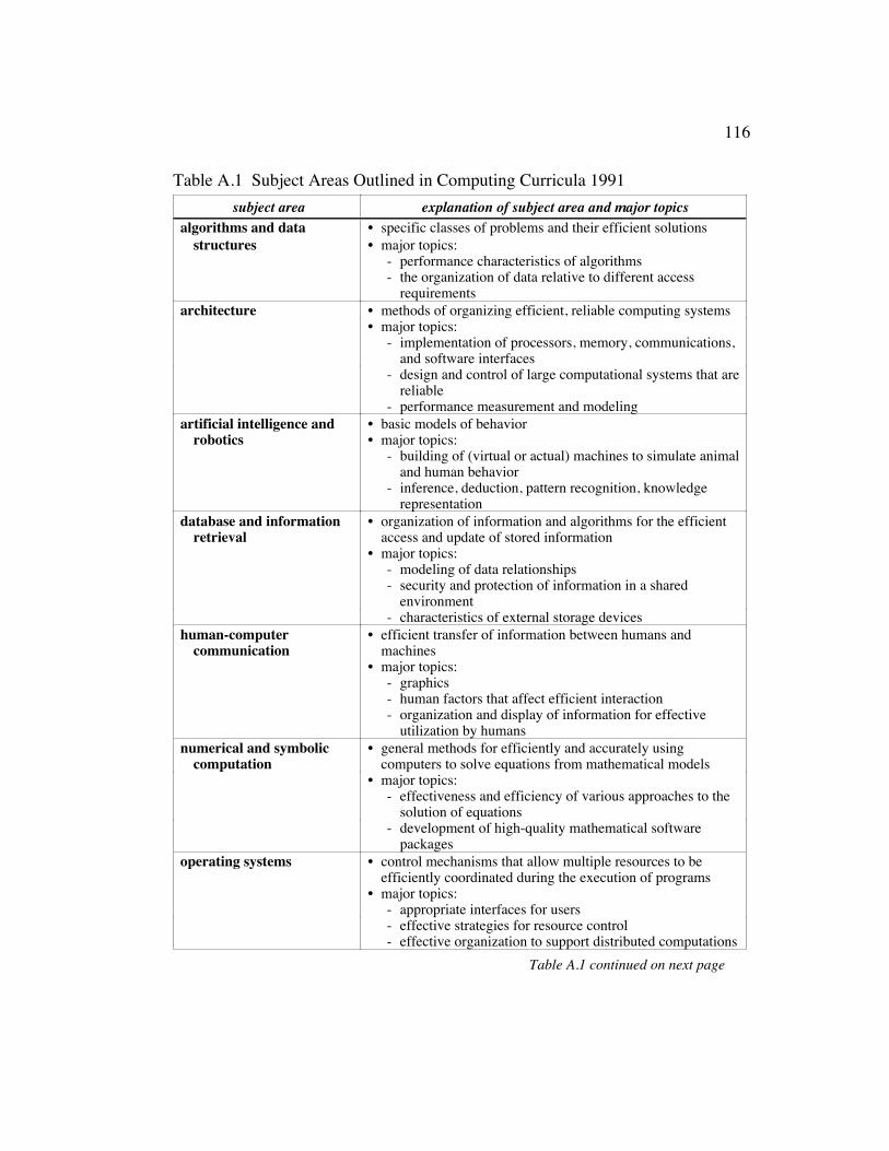
116

Table A.1 Subject Areas Outlined in Computing Curricula 1991subject area explanation of subject area and major topics

algorithms and data • specific classes of problems and their efficient solutionsstructures • major topics:

- performance characteristics of algorithms- the organization of data relative to different access

requirementsarchitecture • methods of organizing efficient, reliable computing systems

• major topics:- implementation of processors, memory, communications,

and software interfaces- design and control of large computational systems that are

reliable- performance measurement and modeling

artificial intelligence and • basic models of behaviorrobotics • major topics:

- building of (virtual or actual) machines to simulate animaland human behavior

- inference, deduction, pattern recognition, knowledgerepresentation

database and informationretrieval

• organization of information and algorithms for the efficientaccess and update of stored information

• major topics:- modeling of data relationships- security and protection of information in a shared

environment- characteristics of external storage devices

human-computercommunication

• efficient transfer of information between humans andmachines

• major topics:- graphics- human factors that affect efficient interaction- organization and display of information for effective

utilization by humansnumerical and symbolic

computation• general methods for efficiently and accurately using

computers to solve equations from mathematical models• major topics:

- effectiveness and efficiency of various approaches to thesolution of equations

- development of high-quality mathematical softwarepackages

operating systems • control mechanisms that allow multiple resources to beefficiently coordinated during the execution of programs

• major topics:- appropriate interfaces for users- effective strategies for resource control- effective organization to support distributed computations

Table A.1 continued on next page

117

Continuation of Table A.1subject area explanation

programming languages • notations for defining virtual machines that executealgorithms

• the efficient translation from high-level to machine codes• various extension mechanisms that can be provided in

programming languagessoftware methodology and

engineering• design and production of large software systems that meet

specifications• major topics:

- principles of programming and software development- verification and validation of software- specification and production of software systems that are

safe, secure, reliable, and dependable

Table A.2 Processes as Defined in Computing Curricula 1991process explanation of process

theory • akin to processes used in mathematics in the development of coherenttheories

• used in developing and understanding the underlying mathematicalprinciples that apply to the discipline of computing

• major elements:- definitions and axioms- theorems- proofs- interpretation of results

abstraction • rooted in the experimental sciences• used when modeling potential algorithms, data structures, architectures, etc.• also used when testing hypotheses about models, alternative design

decisions, or the underlying theory itself• major elements:

- data collection and hypothesis formation- modeling and prediction- design of an experiment- analysis of results

design • rooted in engineering• used in the development of a system or device to solve a given physical

problem• involves conceptualization and realization of systems in the context of real-

world constraints• major elements:

- requirements- specifications- design and implementation- testing and analysis

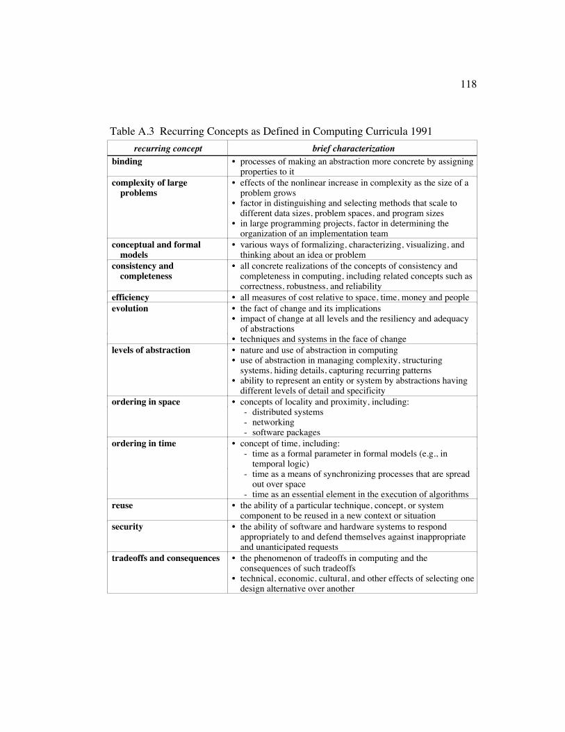
118

Table A.3 Recurring Concepts as Defined in Computing Curricula 1991recurring concept brief characterization

binding • processes of making an abstraction more concrete by assigningproperties to it

complexity of largeproblems

• effects of the nonlinear increase in complexity as the size of aproblem grows

• factor in distinguishing and selecting methods that scale todifferent data sizes, problem spaces, and program sizes

• in large programming projects, factor in determining theorganization of an implementation team

conceptual and formalmodels

• various ways of formalizing, characterizing, visualizing, andthinking about an idea or problem

consistency andcompleteness

• all concrete realizations of the concepts of consistency andcompleteness in computing, including related concepts such ascorrectness, robustness, and reliability

efficiency • all measures of cost relative to space, time, money and peopleevolution • the fact of change and its implications

• impact of change at all levels and the resiliency and adequacyof abstractions

• techniques and systems in the face of changelevels of abstraction • nature and use of abstraction in computing

• use of abstraction in managing complexity, structuringsystems, hiding details, capturing recurring patterns

• ability to represent an entity or system by abstractions havingdifferent levels of detail and specificity

ordering in space • concepts of locality and proximity, including:- distributed systems- networking- software packages

ordering in time • concept of time, including:- time as a formal parameter in formal models (e.g., in

temporal logic)- time as a means of synchronizing processes that are spread

out over space- time as an essential element in the execution of algorithms

reuse • the ability of a particular technique, concept, or systemcomponent to be reused in a new context or situation

security • the ability of software and hardware systems to respondappropriately to and defend themselves against inappropriateand unanticipated requests

tradeoffs and consequences • the phenomenon of tradeoffs in computing and theconsequences of such tradeoffs

• technical, economic, cultural, and other effects of selecting onedesign alternative over another

119

Table A.4 Knowledge Units Comprising the Common Requirements inComputing Curriculum 1991“tag” knowledge unit name

AL algorithms and data structuresAL1 • basic data structuresAL2 • abstract data typesAL3 • recursive algorithmsAL4 • complexity analysisAL5 • complexity classesAL6 • sorting and searchingAL7 • computability and undecidabilityAL8 • problem-solving strategiesAL9 • parallel and distributed algorithms

AR architectureAR1 • digital logicAR2 • digital systemsAR3 • machine-level representation of dataAR4 • assembly-level machine organizationAR5 • memory system organization and

architectureAR6 • interfacing and communicationAR7 • alternative architectures

AI artificial intelligence and roboticsAI1 • history and applications of artificial

intelligenceAI2 • problems, state spaces, and search

strategiesDB database and information retrieval

DB1 • overview, models, and applications ofdatabase systems

DB2 • the relational data modelHU human-computer communication

HU1 • user interfacesHU2 • computer graphics

NU numerical and symbolic computationNU1 • number representation, errors, and

portabilityNU2 • iterative approximation methods

“tag” knowledge unit nameOS operating systems

OS1 • history, evolution, and philosophyOS2 • tasking and processesOS3 • process coordination and

synchronizationOS4 • scheduling and dispatchOS5 • physical and virtual memory

organizationOS6 • device managementOS7 • file systems and namingOS8 • security and protectionOS9 • communications and networking

OS10 • distributed and real-time systemsPL programming languages

PL1 • history and overview of programminglanguages

PL2 • virtual machinesPL3 • representation of data typesPL4 • sequence controlPL5 • data control, sharing, and type

checkingPL6 • run-time storage managementPL7 • finite state automata and regular

expressionsPL8 • context-free grammars and pushdown

automataPL9 • language translation systems

PL10 • programming language semanticsPL11 • programming paradigmsPL12 • distributed and parallel programming

constructsSE software methodology &

engineeringSE1 • fundamental problem-solving conceptsSE2 • the software development processSE3 • software requirements and

specificationsSE4 • software design and implementationSE5 • verification and validation

SP social, ethical, & professional issuesSP1 • historical and social context of

computingSP2 • responsibilities of the computing

professionalSP3 • risks and liabilitiesSP4 • intellectual property

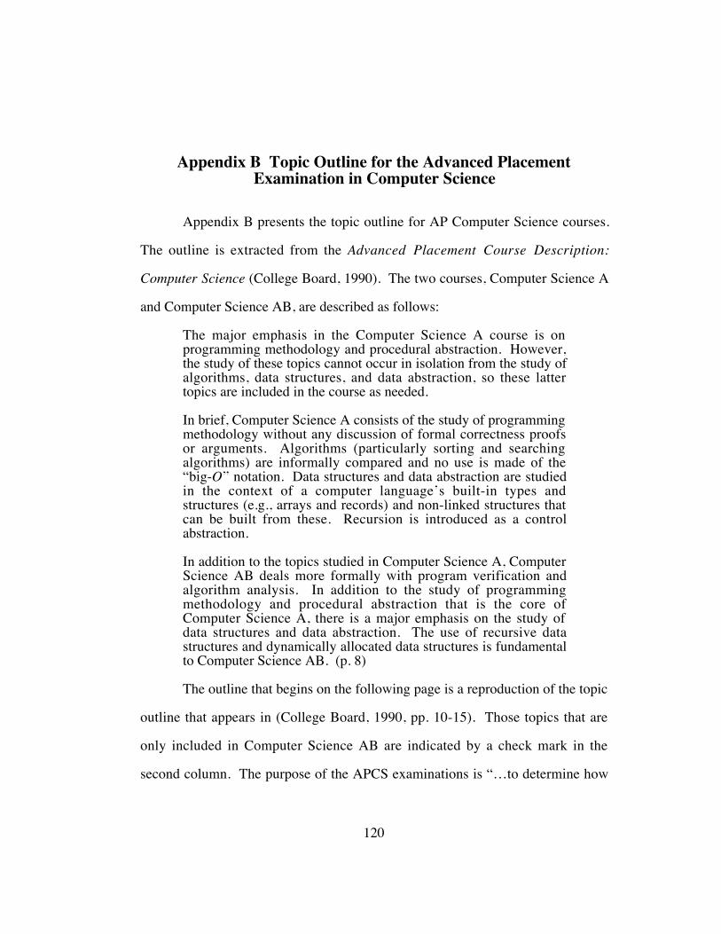
120

Appendix B Topic Outline for the Advanced PlacementExamination in Computer Science

Appendix B presents the topic outline for AP Computer Science courses.

The outline is extracted from the Advanced Placement Course Description:

Computer Science (College Board, 1990). The two courses, Computer Science A

and Computer Science AB, are described as follows:

The major emphasis in the Computer Science A course is onprogramming methodology and procedural abstraction. However,the study of these topics cannot occur in isolation from the study ofalgorithms, data structures, and data abstraction, so these lattertopics are included in the course as needed.

In brief, Computer Science A consists of the study of programmingmethodology without any discussion of formal correctness proofsor arguments. Algorithms (particularly sorting and searchingalgorithms) are informally compared and no use is made of the“big-O” notation. Data structures and data abstraction are studiedin the context of a computer language’s built-in types andstructures (e.g., arrays and records) and non-linked structures thatcan be built from these. Recursion is introduced as a controlabstraction.

In addition to the topics studied in Computer Science A, ComputerScience AB deals more formally with program verification andalgorithm analysis. In addition to the study of programmingmethodology and procedural abstraction that is the core ofComputer Science A, there is a major emphasis on the study ofdata structures and data abstraction. The use of recursive datastructures and dynamically allocated data structures is fundamentalto Computer Science AB. (p. 8)

The outline that begins on the following page is a reproduction of the topic

outline that appears in (College Board, 1990, pp. 10-15). Those topics that are

only included in Computer Science AB are indicated by a check mark in the

second column. The purpose of the APCS examinations is “…to determine how

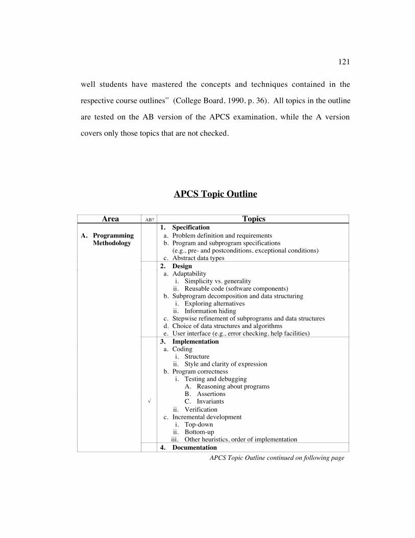
121

well students have mastered the concepts and techniques contained in the

respective course outlines” (College Board, 1990, p. 36). All topics in the outline

are tested on the AB version of the APCS examination, while the A version

covers only those topics that are not checked.

APCS Topic Outline

Area AB? Topics1. Specification

A. ProgrammingMethodology

a. Problem definition and requirementsb. Program and subprogram specifications

(e.g., pre- and postconditions, exceptional conditions)c. Abstract data types

2. Designa. Adaptability

i. Simplicity vs. generalityii. Reusable code (software components)

b. Subprogram decomposition and data structuringi. Exploring alternatives

ii. Information hidingc. Stepwise refinement of subprograms and data structuresd. Choice of data structures and algorithmse. User interface (e.g., error checking, help facilities)

3. Implementationa. Coding

i. Structureii. Style and clarity of expression

b. Program correctnessi. Testing and debugging

A. Reasoning about programsB. Assertions

√ C. Invariantsii. Verification

c. Incremental developmenti. Top-down

ii. Bottom-upiii. Other heuristics, order of implementation

4. DocumentationAPCS Topic Outline continued on following page

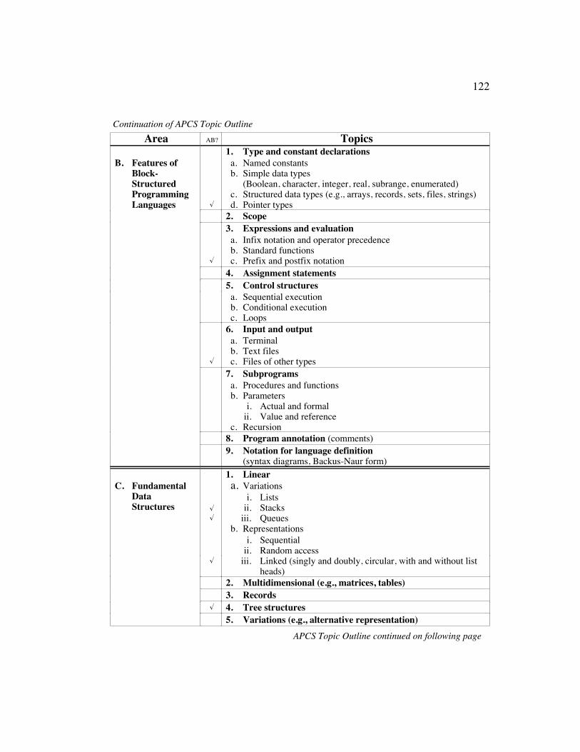
122

Continuation of APCS Topic OutlineArea AB? Topics

1. Type and constant declarationsB. Features of

Block-StructuredProgrammingLanguages √

a. Named constantsb. Simple data types

(Boolean, character, integer, real, subrange, enumerated)c. Structured data types (e.g., arrays, records, sets, files, strings)d. Pointer types

2. Scope3. Expressions and evaluationa. Infix notation and operator precedenceb. Standard functions

√ c. Prefix and postfix notation4. Assignment statements5. Control structuresa. Sequential executionb. Conditional executionc. Loops

6. Input and outputa. Terminalb. Text files

√ c. Files of other types7. Subprogramsa. Procedures and functionsb. Parameters

i. Actual and formalii. Value and reference

c. Recursion8. Program annotation (comments)9. Notation for language definition

(syntax diagrams, Backus-Naur form)1. Linear

C. FundamentalDataStructures √

√

a. Variationsi. Lists

ii. Stacksiii. Queues

b. Representationsi. Sequential

ii. Random access√ iii. Linked (singly and doubly, circular, with and without list

heads)2. Multidimensional (e.g., matrices, tables)3. Records

√ 4. Tree structures5. Variations (e.g., alternative representation)

APCS Topic Outline continued on following page

123

Continuation of APCS Topic OutlineArea AB? Topics

1. Operations on fundamental data structuresD. Algorithms a. Insertion

b. Deletionc. Traversals

2. Searching

√√

a. Sequential (linear) searchb. Binary searchc. Hashingd. Searching an ordered binary tree

3. Sortinga. Quadratic sortsb. More efficient sorts

√√√

4. Analysis of algorithmsa. Informal comparison of speedsb. The meaning of “big-O” notationc. Worst-case timed. Worst-case space

√√√√√

5. Numerical algorithmsa. Approximations (e.g., zeros of functions, Monte Carlo method)b. Numerical accuracy

i. Round-off effectsii. Precision of approximations

1. Major hardware componentsE. Computer

Systemsa. Primary and secondary memoryb. Processorsc. Peripherals

2. System softwarea. Language translatorsb. Operating systemsc. File systems

3. Types of systemsa. Single-user systemsb. Time-sharing and batch-processing systemsc. Networks

F. ResponsibleUse ofComputerSystems

1. Privacy2. Reliability of systems3. Legal issues and intellectual property4. Social ramifications of computer applications

Note: From Advanced Placement Course Description: Computer Science, College EntranceExamination Board, 1990 (May 1991 version), pp. 10-14. Adapted by permission.

124

Appendix C Taxonomy of Concepts in the Computer ScienceSubdomain Two-Valued Logic

Appendix C presents the full taxonomy of concepts in the computer

science subdomain of mathematical logic that was developed for this study. The

taxonomy fills in the details for the high-level pictorial outline that was given as

the Quick Reference to the Concepts of “Two-Valued Logic” in Figure 3.1 of

Chapter 3. The qualifying phrase “two-valued” was used to emphasize the sort of

mathematical logic that was under consideration in this research, that is, logic

restricted to a two-valued domain.

125

Full Taxonomy of Conceptsin the Computer Science Subdomain Two-Valued Logic

1.0 Datatype boolean1.1 Set of values {true, false}1.2 Set of operations { equal" (=), not" (ÿ),

and" (Ÿ), or" (⁄), implies" (fi), …}1.2.1 Truth tables1.2.2 Precedence rules

1.3 Properties1.3.1 Non-numeric1.3.2 Unordered1.3.3 Discrete

2.0 Related simple datatypes2.1 Bit

2.1.1 Set of values {0, 1}2.1.2 Set of operations { equal , +, *,

in-order , …}2.1.3 Properties

2.1.3.1 Numeric2.1.3.2 Ordered2.1.3.3 Discrete2.1.3.4 Bounded

2.2 State, restricted to two values2.2.1 Set of values: Any set of two distinct

literal values (e.g., {on, off}, {left,right})

2.2.2 Set of operations { equal , toggle , …}2.2.3 Properties

2.2.3.1 Non-numeric2.2.3.2 Unordered2.2.3.3 Discrete

2.3 Two-valued subrange of integer

3.0 Boolean-based calculi3.1 Boolean variables or identifiers3.2 States (associating identifiers with values)3.3 Propositions3.4 Tautologies3.5 Quantification3.6 Bound vs. free variables3.7 Predicates3.8 Functions3.9 Laws {equivalence, commutative,

associative, distributive, De Morgan’s, …}3.10 Axioms, inference rules, theorems

4.0 Boolean aspects of ProgrammingLanguages

4.1 Realization of datatype boolean4.2 Boolean expressions

4.2.1 Constants and named constants4.2.2 Relations (functions of other datatypes

yielding boolean values)4.2.3 “Predicate calculus expressions”

(functions of boolean values yieldingboolean values)

4.2.4 Boolean-valued function calls4.3 Assignment with datatype boolean

4.3.1 rvalues: [named] constant, variable,…

4.3.2 lvalues: variable, field, attribute,property, …

4.4 Conditional control structures in imperativelanguages

4.4.1 Selection4.4.1.1 Explicit boolean condition

(e.g., if )4.4.1.2 Implicit boolean condition

(e.g. case in Pascal)4.4.2 Iteration

4.4.2.1 Explicit boolean condition(e.g., while & repeat inPascal; for in C)

4.4.2.2 implicit boolean condition(e.g., for in Pascal)

4.5 Parameters of type boolean4.6 Other uses in non-imperative languages

4.6.1 Constraints in descriptive ordeclarative languages

4.6.2 Explicit third value, i.e. {true, false,null/no value}

5.0 Assertions & Formal Verification5.1 Precondition / postcondition5.2 Loop invariant5.3 Calculation of weakest precondition5.4 Data transformations

6.0 Other Topics / Advanced Topics6.1 Boolean structures6.2 Deduction systems6.3 Constructivist logic / 3-valued logic

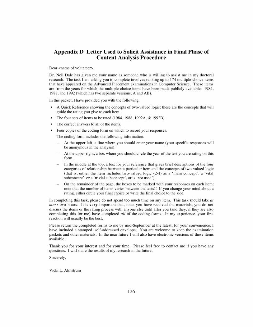
126

Appendix D Letter Used to Solicit Assistance in Final Phase ofContent Analysis Procedure

Dear <name of volunteer>,Dr. Nell Dale has given me your name as someone who is willing to assist me in my doctoralresearch. The task I am asking you to complete involves ranking up to 174 multiple-choice itemsthat have appeared on the Advanced Placement examinations in Computer Science. These itemsare from the years for which the multiple-choice items have been made publicly available: 1984,1988, and 1992 (which has two separate versions, A and AB).In this packet, I have provided you with the following:• A Quick Reference showing the concepts of two-valued logic; these are the concepts that will

guide the rating you give to each item.• The four sets of items to be rated (1984, 1988, 1992A, & 1992B).• The correct answers to all of the items.• Four copies of the coding form on which to record your responses.

The coding form includes the following information:– At the upper left, a line where you should enter your name (your specific responses will

be anonymous in the analysis).– At the upper right, a box where you should circle the year of the test you are rating on this

form.– In the middle at the top, a box for your reference that gives brief descriptions of the four

categories of relationship between a particular item and the concepts of two-valued logic(that is, either the item includes two-valued logic (2vl) as a ‘main concept’, a ‘vitalsubconcept’, or a ‘trivial subconcept’, or is ‘not used’).

– On the remainder of the page, the boxes to be marked with your responses on each item;note that the number of items varies between the tests!! If you change your mind about arating, either circle your final choice or write the final choice to the side.

In completing this task, please do not spend too much time on any item. This task should take atmost two hours. It is very important that, once you have received the materials, you do notdiscuss the items or the rating process with anyone else until after you (and they, if they are alsocompleting this for me) have completed all of the coding forms. In my experience, your firstreaction will usually be the best.Please return the completed forms to me by mid-September at the latest; for your convenience, Ihave included a stamped, self-addressed envelope. You are welcome to keep the examinationpackets and other materials. In the near future I will also have electronic versions of these itemsavailable.Thank you for your interest and for your time. Please feel free to contact me if you have anyquestions. I will share the results of my research in the future.Sincerely,

Vicki L. Almstrum

127

Appendix E Coding Form for Content Analysis Procedure

Appendix E gives the coding form that was used during the final phase of

the content analysis procedure. Key features of the coding form are the

following:

• The form design allowed one layout to be used for rating any of the

examination packets. Judges were instructed to circle the appropriate

examination packet year in the upper right-hand corner of the form.

• As an aid, the number of items in each examination packet was given

beneath the examination packet years in the upper right-hand corner.

• The judge’s name was to be entered at the upper left-hand corner of the

form. The researcher assigned a unique identification code to each judge,

allowing a particular judge’s ratings across examination packets to be

traced. All identifying information was kept in confidence so that a

particular judge could not be identified based simply on the reported

responses.

• Simple clarification of the instructions for completing the classification

procedure was given at the top of the form, including the classification

categories.

The primary criticism of the form as given was the absence of item numbers along

the right side of each column, mirroring those given at the left. It was felt that the

extra column would have made it easier for the judge to check the appropriate

box. If the form is used again, it should be modified by repeating the first column

as the last column.

128

129

Appendix F Item Assignment to Strongly Related and NotStrongly Related Partitions under each Partitioning Algorithm

Appendix F reports the item-by-item assignment to partitions for all of the

examination packets. Tables F.1 through F.4 provide detailed information about

the 1984, 1988, 1992 version A, and 1992 version AB examination packets,

respectively. Each table reports, per item, the number of judges who chose the

strongly related classifications (‘main concept’ or ‘vital subconcept’) and the not

strongly related classifications (‘trivial subconcept’ or ‘not used’). These two

figures were the basis for assigning the item to a partition under each of the two

partitioning algorithms; an item’s partition assignment under each partitioning

algorithm is shown symbolically immediately to the right of the item number in

the table.

The partitioning algorithms were as follows:

• Under the liberal partitioning algorithm, an item was classified as strongly

related if 50% of the judges had rated the item as ‘main concept’ or ‘vital

subconcept’ and not strongly related otherwise.

• Under the conservative partitioning algorithm, an item was classified as

strongly related if at least 75% of the judges had rated it as ‘main concept’

or ‘vital subconcept’. If fewer than 25% of the judges rated the item as

‘main concept’ or ‘vital subconcept’, it was classified as not strongly

related. Under the conservative partitioning algorithm, items in the mid-

range of agreement were eliminated from further consideration.

130

Table F.1 Number of Judges Choosing Specific Categories for Each Item andAssignment of Items to Partitions under Each Partitioning Algorithm for 1984APCS Examination

item number and item number andpartition indicators # of judges choosing … partition

indicators# of judges choosing …

under liberal andconservativealgorithms

main conceptor vital

subconcept

trivialsubconceptor not used

under liberal andconservativealgorithms

main conceptor vital

subconcept

trivialsubconceptor not used

1984-01 * • 0 38 1984-23 * • 0 381984-02 † – 24 14 1984-24 * • 0 381984-03 * • 2 36 1984-25 † – 28 101984-04 * • 4 34 1984-26 * • 1 371984-05 * • 1 37 1984-27 * • 0 381984-06 * • 5 33 1984-28 * • 0 381984-07 * • 0 38 1984-29 * • 0 381984-08 † – 25 13 1984-30 † – 23 151984-09 * • 8 30 1984-31 * • 2 361984-10 * • 2 36 1984-32 * • 1 371984-11 * • 2 36 1984-33 * • 9 291984-12 † – 27 11 1984-34 * • 8 301984-13 * • 6 32 1984-35 * – 10 281984-14 * • 4 34 1984-36 * – 14 241984-15 * • 0 38 1984-37 * – 17 211984-16 † ‡ 29 9 1984-38 * • 9 291984-17 † ‡ 38 0 1984-39 * • 1 371984-18 † – 24 14 1984-40 * • 4 341984-19 * – 14 24 1984-41 † ‡ 30 81984-20 * • 0 38 1984-42 † ‡ 37 11984-21 * • 2 36 1984-43 * • 2 361984-22 * • 2 36 1984-44 * • 3 35

Note: number of judges = 38

Key to partition indicators: First column of symbols after the item number: liberal algorithm, where:

† means the item is in strongly related partition* means the item is in not strongly related partition

Second column of symbols after the item number: conservative algorithm, where:‡ means the item is in strongly related partition• means the item is in not strongly related partition– means the item is excluded from consideration

131

Table F.2 Number of Judges Choosing Specific Categories for Each Item andAssignment of Items to Partitions under Each Partitioning Algorithm for 1988APCS Examination

item number and item number andpartition indicators # of judges choosing … partition

indicators# of judges choosing …

under liberal andconservativealgorithms

main conceptor vital

subconcept

trivialsubconceptor not used

under liberal andconservativealgorithms

main conceptor vital

subconcept

trivialsubconceptor not used

1988-01 * • 0 36 1988-26 * • 1 351988-02 * • 0 36 1988-27 * • 1 351988-03 * • 1 35 1988-28 * • 1 351988-04 * • 4 32 1988-29 * – 12 241988-05 † ‡ 28 8 1988-30 * • 1 351988-06 † ‡ 33 3 1988-31 * • 1 351988-07 * • 0 36 1988-32 † – 19 171988-08 * • 0 36 1988-33 * – 9 271988-09 * • 0 36 1988-34 * • 2 341988-10 * • 2 34 1988-35 * • 3 331988-11 * – 12 24 1988-36 * • 0 361988-12 † – 24 12 1988-37 * • 0 361988-13 † – 18 18 1988-38 * • 4 321988-14 † ‡ 32 4 1988-39 * • 7 291988-15 † – 24 12 1988-40 † – 19 171988-16 † – 18 18 1988-41 * • 6 301988-17 * – 12 24 1988-42 * • 0 361988-18 † – 26 10 1988-43 * • 1 351988-19 * – 12 24 1988-44 † ‡ 30 61988-20 * – 11 25 1988-45 * • 0 361988-21 * • 1 35 1988-46 * • 8 281988-22 † – 20 16 1988-47 * • 3 331988-23 † ‡ 35 1 1988-48 * • 1 351988-24 * • 0 36 1988-49 * • 3 331988-25 * – 17 19 1988-50 † – 23 13

Note: number of judges = 36; version A is items 1-35 and version AB is all 50 itemsKey to partition indicators: First column of symbols after the item number: liberal algorithm, where:

† means the item is in strongly related partition* means the item is in not strongly related partition

Second column of symbols after the item number: conservative algorithm, where:‡ means the item is in strongly related partition• means the item is in not strongly related partition

132

– means the item is excluded from consideration

133

Table F.3 Number of Judges Choosing Specific Categories for Each Item andAssignment of Items to Partitions under Each Partitioning Algorithm for 1992APCS Examination, Version A

item number and item number andpartition indicators # of judges choosing … partition

indicators# of judges choosing …

under liberal andconservativealgorithms

main conceptor vital

subconcept

trivialsubconceptor not used

under liberal andconservativealgorithms

main conceptor vital

subconcept

trivialsubconceptor not used

1992A-01 * • 4 34 1992A-21 † – 26 121992A-02 * • 3 35 1992A-22 † – 19 191992A-03 * • 0 38 1992A-23 * • 2 361992A-04 * – 14 24 1992A-24 † ‡ 32 61992A-05 * – 11 27 1992A-25 † – 25 131992A-06 * • 1 37 1992A-26 † ‡ 38 01992A-07 * • 1 37 1992A-27 † ‡ 37 11992A-08 † – 28 10 1992A-28 * • 3 351992A-09 * – 15 23 1992A-29 * – 16 221992A-10 * – 16 22 1992A-30 † ‡ 29 91992A-11 † – 26 12 1992A-31 † ‡ 38 01992A-12 † ‡ 37 1 1992A-32 † ‡ 38 01992A-13 † – 26 12 1992A-33 * – 18 201992A-14 * – 17 21 1992A-34 * • 5 331992A-15 * – 15 23 1992A-35 † ‡ 31 71992A-16 † – 27 11 1992A-36 * – 15 231992A-17 * – 16 22 1992A-37 * • 2 361992A-18 * • 9 29 1992A-38 * • 2 361992A-19 * – 10 28 1992A-39 * • 1 371992A-20 † – 28 10 1992A-40 * • 9 29

Note: number of judges = 38

Key to partition indicators: First column of symbols after the item number: liberal algorithm, where:

† means the item is in strongly related partition* means the item is in not strongly related partition

Second column of symbols after the item number: conservative algorithm, where:‡ means the item is in strongly related partition• means the item is in not strongly related partition– means the item is excluded from consideration

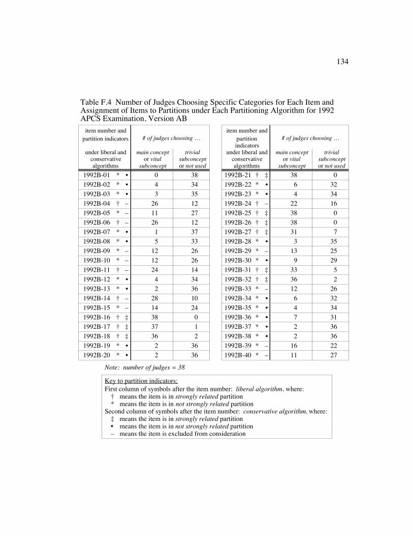
134

Table F.4 Number of Judges Choosing Specific Categories for Each Item andAssignment of Items to Partitions under Each Partitioning Algorithm for 1992APCS Examination, Version AB

item number and item number andpartition indicators # of judges choosing … partition

indicators# of judges choosing …

under liberal andconservativealgorithms

main conceptor vital

subconcept

trivialsubconceptor not used

under liberal andconservativealgorithms

main conceptor vital

subconcept

trivialsubconceptor not used

1992B-01 * • 0 38 1992B-21 † ‡ 38 01992B-02 * • 4 34 1992B-22 * • 6 321992B-03 * • 3 35 1992B-23 * • 4 341992B-04 † – 26 12 1992B-24 † – 22 161992B-05 * – 11 27 1992B-25 † ‡ 38 01992B-06 † – 26 12 1992B-26 † ‡ 38 01992B-07 * • 1 37 1992B-27 † ‡ 31 71992B-08 * • 5 33 1992B-28 * • 3 351992B-09 * – 12 26 1992B-29 * – 13 251992B-10 * – 12 26 1992B-30 * • 9 291992B-11 † – 24 14 1992B-31 † ‡ 33 51992B-12 * • 4 34 1992B-32 † ‡ 36 21992B-13 * • 2 36 1992B-33 * – 12 261992B-14 † – 28 10 1992B-34 * • 6 321992B-15 * – 14 24 1992B-35 * • 4 341992B-16 † ‡ 38 0 1992B-36 * • 7 311992B-17 † ‡ 37 1 1992B-37 * • 2 361992B-18 † ‡ 36 2 1992B-38 * • 2 361992B-19 * • 2 36 1992B-39 * – 16 221992B-20 * • 2 36 1992B-40 * – 11 27

Note: number of judges = 38

Key to partition indicators: First column of symbols after the item number: liberal algorithm, where:

† means the item is in strongly related partition* means the item is in not strongly related partition

Second column of symbols after the item number: conservative algorithm, where:‡ means the item is in strongly related partition• means the item is in not strongly related partition– means the item is excluded from consideration

135

136

Appendix G Multiple-Choice Items in the Strongly RelatedPartition Defined by the Conservative Partitioning Algorithm

Appendix G presents the full text of several multiple-choice items from

the Advanced Placement Examinations in Computer Science for 1984, 1988, and

1992. The items included in this appendix are those that, after the final phase of

the content analysis procedure was completed, were classified as strongly related

under the conservative partitioning algorithm.

Twenty-two multiple-choice items are included in Appendix G. The

sources of the items are as follows:

• 4 items from the 1984 examination(1984-16, 1984-17, 1984-41, 1984-42)

• 5 items from the 1988 examination(1988-5, 1988-6, 1988-14, 1988-23, 1988-44)

• 4 items from the A version of the 1992 examination(1992A-12, 1992A-24, 1992A-30, 1992A-35)

• 5 items from the AB version of the 1992 examination(1992B-25, 1992B-26, 1992B-27, 1992B-31, 1992B-32)

• 4 items that were common to both versions of the 1992 examination(1992A-26 = 1992B-16, 1992A-27 = 1992B-17, 1992A-31 = 1992B-18, 1992A-32 = 1992B-21)

Because the items are being presented outside of the context of the

examination packet, some minor changes have been made to the introductory

wording for some items. Such changes were purely cosmetic and had no effect on

the content of the multiple-choice item.

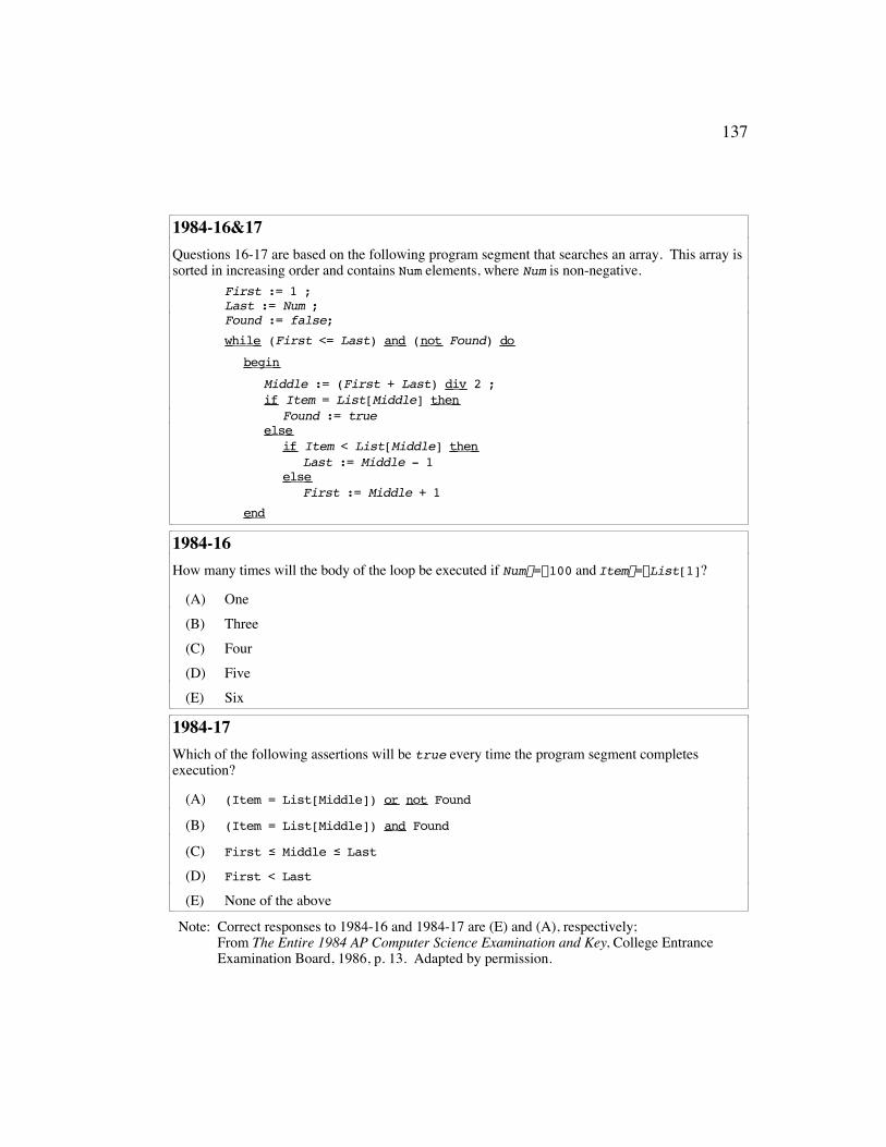
137

1984-16&17Questions 16-17 are based on the following program segment that searches an array. This array issorted in increasing order and contains Num elements, where Num is non-negative.

First := 1 ;Last := Num ;Found := false; while (First <= Last) and ( not Found) do

begin

Middle := (First + Last) div 2 ; if Item = List[Middle] then

Found := true else

if Item < List[Middle] then Last := Middle - 1

else First := Middle + 1

end

1984-16How many times will the body of the loop be executed if Num#=#100 and Item#=#List[1]?

(A) One(B) Three(C) Four(D) Five(E) Six

1984-17Which of the following assertions will be true every time the program segment completesexecution?

(A) (Item = List[Middle]) or not Found

(B) (Item = List[Middle]) and Found

(C) First ≤ Middle ≤ Last

(D) First < Last

(E) None of the above

Note: Correct responses to 1984-16 and 1984-17 are (E) and (A), respectively;From The Entire 1984 AP Computer Science Examination and Key, College EntranceExamination Board, 1986, p. 13. Adapted by permission.

138

1984-41Let x and y be variables of type real with only positive values. Of the following, which bestdescribes the conditions under which the boolean expression, x + y = x, can have the valuetrue?

(A) Only when y > x(B) Only when y < 1(C) Only when x is much greater than y(D) Only when the computer has 16-bit words(E) It can never have the value true

Note: Correct response to 1984-41 is (C); From The Entire 1984 AP Computer ScienceExamination and Key, College Entrance Examination Board, 1986, p. 27. Adapted bypermission.

1984-42i := 1 ; while (i <= Max) and (String[i] <> Symbol) do i := i + 1

Which of the following is a loop invariant for the while loop above; i.e., which is true each timethe while -condition is tested?

(A) i = Max

(B) i = i + 1

(C) String[j] = Symbol for all j such that i < j

(D) String[j] ≠ Symbol for all j such that i ≤ j

(E) String[j] ≠ Symbol for all j such that 1 ≤ j < i

Note: Correct response to 1984-42 is (E); From The Entire 1984 AP Computer ScienceExamination and Key, College Entrance Examination Board, 1986, p. 27. Adapted bypermission.

139

1988-5If evaluating BBB has no side effects, under what condition(s) can the program segment

while BBB do

Block1

be rewritten as repeat

Block1 until not BBB

Without changing the effect of the code?

(A) Under no conditions(B) If executing Block1 does not affect the value of BBB(C) If the value of BBB is true just before the segment is executed(D) If the value of BBB is false just before the segment is executed(E) Under all conditions

Note: Correct response to 1988-5 is (C); From The 1988 Advanced Placement Examinations inComputer Science and their grading, College Entrance Examination Board, 1989, p. 6.Adapted by permission.

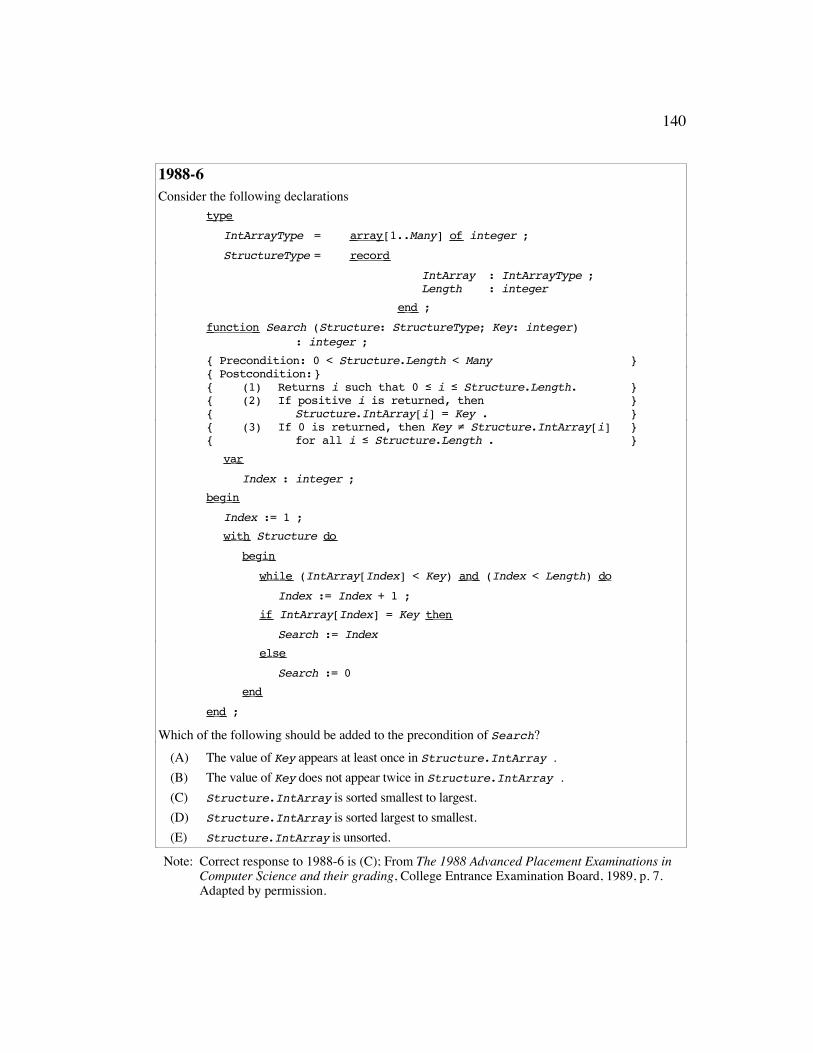
140

1988-6Consider the following declarations

type

IntArrayType = array [1..Many] of integer ;

StructureType = record

IntArray : IntArrayType ;Length : integer

end ;

function Search (Structure: StructureType; Key: integer): integer ;

{ Precondition: 0 < Structure.Length < Many }{ Postcondition:}{ (1) Returns i such that 0 ≤ i ≤ Structure.Length. }{ (2) If positive i is returned, then }{ Structure.IntArray[i] = Key . }{ (3) If 0 is returned, then Key ≠ Structure.IntArray[i] }{ for all i ≤ Structure.Length . }

var

Index : integer ; begin

Index := 1 ; with Structure do

begin

while (IntArray[Index] < Key) and (Index < Length) do

Index := Index + 1 ; if IntArray[Index] = Key then

Search := Index else

Search := 0 end

end ;

Which of the following should be added to the precondition of Search?(A) The value of Key appears at least once in Structure.IntArray .(B) The value of Key does not appear twice in Structure.IntArray .(C) Structure.IntArray is sorted smallest to largest.(D) Structure.IntArray is sorted largest to smallest.(E) Structure.IntArray is unsorted.

Note: Correct response to 1988-6 is (C); From The 1988 Advanced Placement Examinations inComputer Science and their grading, College Entrance Examination Board, 1989, p. 7.Adapted by permission.

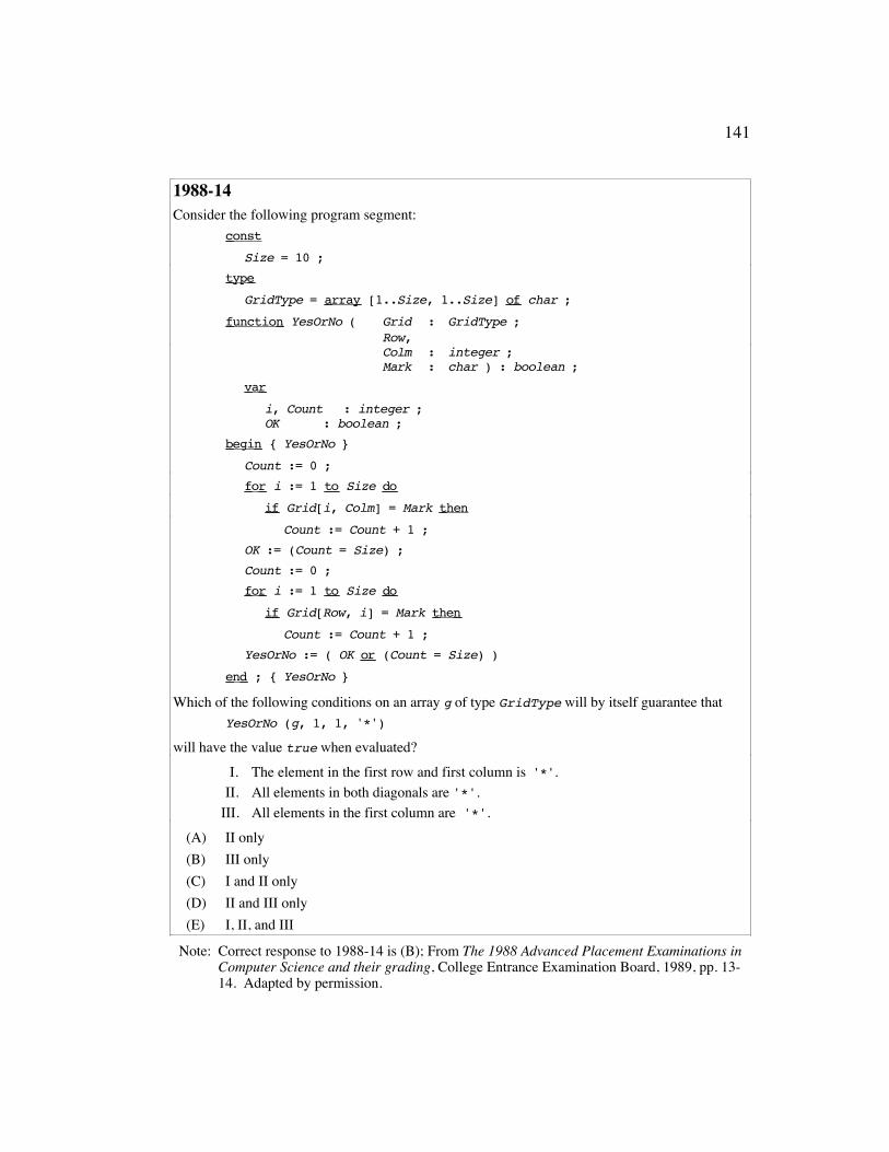
141

1988-14Consider the following program segment:

const

Size = 10 ; type

GridType = array [1..Size, 1..Size] of char ;

function YesOrNo ( Grid : GridType ;Row,Colm : integer ;Mark : char ) : boolean ;

var

i, Count : integer ;OK : boolean ;

begin { YesOrNo }

Count := 0 ; for i := 1 to Size do

if Grid[i, Colm] = Mark then

Count := Count + 1 ;OK := (Count = Size) ;Count := 0 ; for i := 1 to Size do

if Grid[Row, i] = Mark then

Count := Count + 1 ;YesOrNo := ( OK or (Count = Size) )

end ; { YesOrNo }

Which of the following conditions on an array g of type GridType will by itself guarantee thatYesOrNo (g, 1, 1, '*')

will have the value true when evaluated?I. The element in the first row and first column is '*'.

II. All elements in both diagonals are '*'.III. All elements in the first column are '*'.

(A) II only(B) III only(C) I and II only(D) II and III only(E) I, II, and III

Note: Correct response to 1988-14 is (B); From The 1988 Advanced Placement Examinations inComputer Science and their grading, College Entrance Examination Board, 1989, pp. 13-14. Adapted by permission.

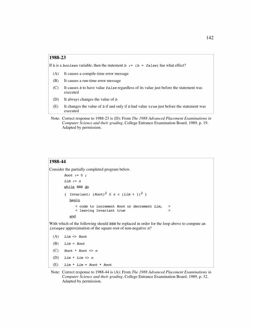
142

1988-23If b is a boolean variable, then the statement b := (b = false) has what effect?

(A) It causes a compile-time error message(B) It causes a run-time error message(C) It causes b to have value false regardless of its value just before the statement was

executed(D) It always changes the value of b(E) It changes the value of b if and only if b had value true just before the statement was

executed

Note: Correct response to 1988-23 is (D); From The 1988 Advanced Placement Examinations inComputer Science and their grading, College Entrance Examination Board, 1989, p. 19.Adapted by permission.

1988-44Consider the partially completed program below.

Root := 0 ;Lim := n while BBB do

{ Invariant: (Root)2 ≤ n < (Lim + 1)2 } begin

< code to increment Root or decrement Lim, >< leaving Invariant true >

end

With which of the following should BBB be replaced in order for the loop above to compute aninteger approximation of the square root of non-negative n?

(A) Lim <> Root

(B) Lim = Root

(C) Root * Root <> n

(D) Lim * Lim <> n

(E) Lim * Lim = Root * Root

Note: Correct response to 1988-44 is (A); From The 1988 Advanced Placement Examinations inComputer Science and their grading, College Entrance Examination Board, 1989, p. 32.Adapted by permission.

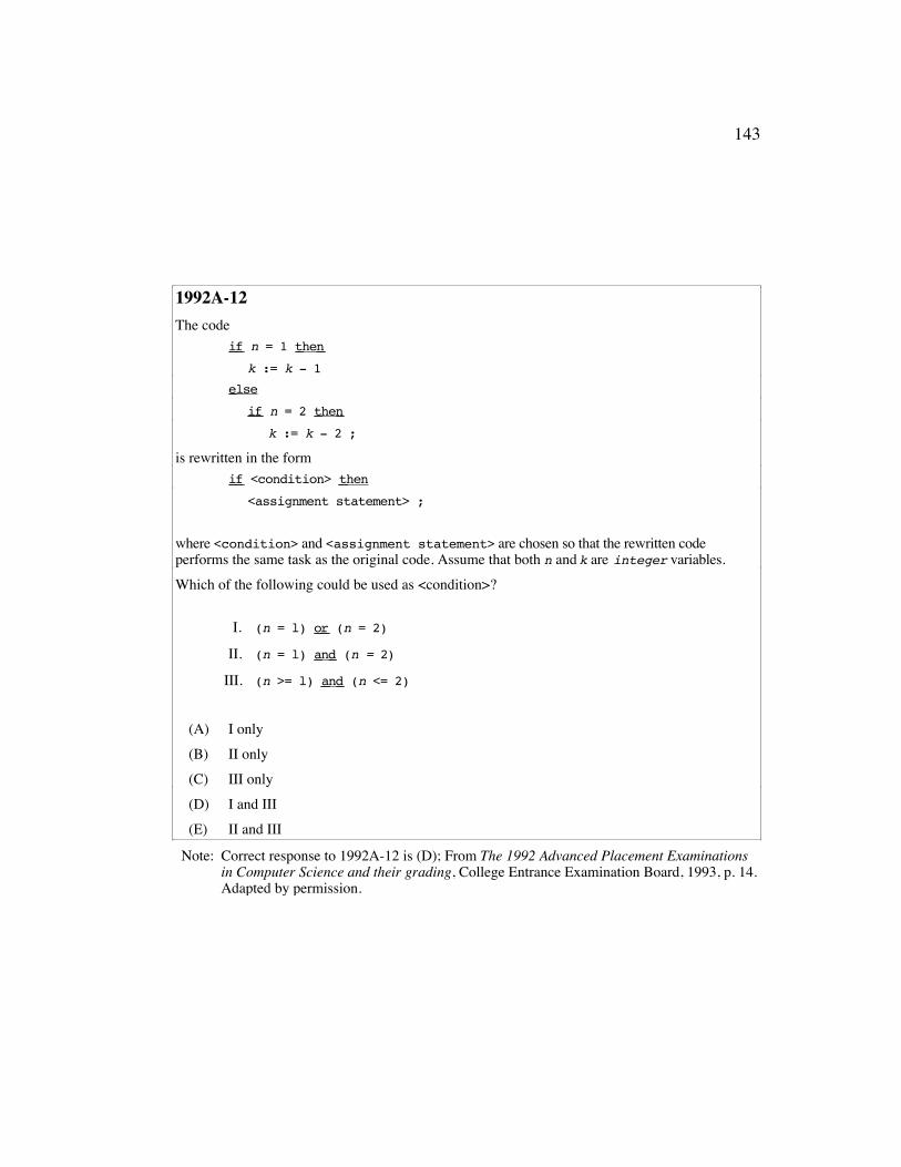
143

1992A-12The code

if n = 1 then

k := k - 1 else

if n = 2 then

k := k - 2 ;

is rewritten in the form if <condition> then

<assignment statement> ;

where <condition> and <assignment statement> are chosen so that the rewritten codeperforms the same task as the original code. Assume that both n and k are integer variables.Which of the following could be used as <condition>?

I. (n = l) or (n = 2)

II. (n = l) and (n = 2)

III. (n >= l) and (n <= 2)

(A) I only(B) II only(C) III only(D) I and III(E) II and III

Note: Correct response to 1992A-12 is (D); From The 1992 Advanced Placement Examinationsin Computer Science and their grading, College Entrance Examination Board, 1993, p. 14.Adapted by permission.

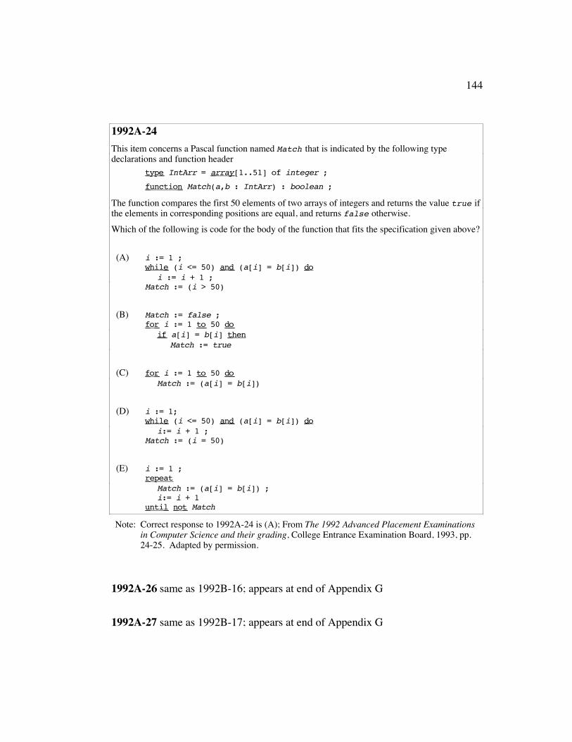
144

1992A-24This item concerns a Pascal function named Match that is indicated by the following typedeclarations and function header

type IntArr = array [1..51] of integer ;

function Match(a,b : IntArr) : boolean ;

The function compares the first 50 elements of two arrays of integers and returns the value true ifthe elements in corresponding positions are equal, and returns false otherwise.Which of the following is code for the body of the function that fits the specification given above?

(A) i := 1 ; while (i <= 50) and (a[i] = b[i]) do

i := i + 1 ;Match := (i > 50)

(B) Match := false ; for i := 1 to 50 do

if a[i] = b[i] thenMatch := true

(C) for i := 1 to 50 do Match := (a[i] = b[i])

(D) i := 1; while (i <= 50) and (a[i] = b[i]) do

i:= i + 1 ;Match := (i = 50)

(E) i := 1 ; repeat

Match := (a[i] = b[i]) ;i:= i + 1

until not Match

Note: Correct response to 1992A-24 is (A); From The 1992 Advanced Placement Examinationsin Computer Science and their grading, College Entrance Examination Board, 1993, pp.24-25. Adapted by permission.

1992A-26 same as 1992B-16; appears at end of Appendix G

1992A-27 same as 1992B-17; appears at end of Appendix G

145

146

1992A-30Consider the following code fragments, where all variables are of type integer.

Fragment 1 Fragment 2 x := n ; x := n ; y := x ; y := x ; while x > 0 do if x > 0 then begin begin y := y + l ; repeat x := x div 2 ; y := y + l; end ; x := x div 2; until x < 0 ; end ;

Assume that the two fragments start with the same value for variable n. For which value(s) of n dothe two code fragments compute the same value for variable y?

I. Any value less than zeroII. The value zero

III. Any value greater than zero

(A) I only(B) II only(C) III only(D) I and II only(E) I, II, and III

Note: Correct response to 1992A-30 is (D); From The 1992 Advanced Placement Examinationsin Computer Science and their grading, College Entrance Examination Board, 1993, p. 30.Adapted by permission.

1992A-31 same as 1992B-21; appears at end of Appendix G

1992A-32 same as 1992B-22; appears at end of Appendix G

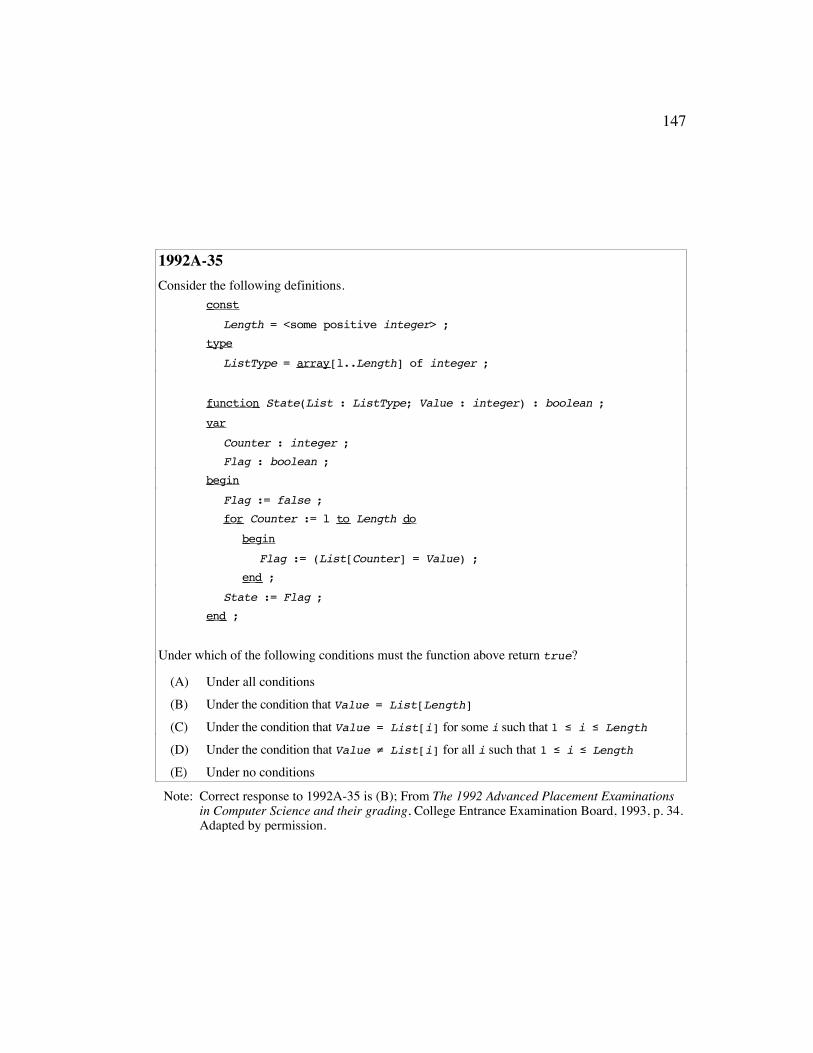
147

1992A-35Consider the following definitions.

const

Length = <some positive integer> ; type

ListType = array [l..Length] of integer ;

function State(List : ListType; Value : integer) : boolean ;

var

Counter : integer ;Flag : boolean ;

begin

Flag := false ; for Counter := l to Length do

begin

Flag := (List[Counter] = Value) ; end ;

State := Flag ; end ;

Under which of the following conditions must the function above return true?

(A) Under all conditions(B) Under the condition that Value = List[Length](C) Under the condition that Value = List[i] for some i such that 1 ≤ i ≤ Length(D) Under the condition that Value ≠ List[i] for all i such that 1 ≤ i ≤ Length(E) Under no conditions

Note: Correct response to 1992A-35 is (B); From The 1992 Advanced Placement Examinationsin Computer Science and their grading, College Entrance Examination Board, 1993, p. 34.Adapted by permission.

148

1992B-16 same as 1992A-26; appears at end of Appendix G1992B-17 same as 1992A-27; appears at end of Appendix G1992B-18 same as 1992A-31; appears at end of Appendix G1992B-21 same as 1992A-32; appears at end of Appendix G

1992B-25&26These questions concern the definition of two new boolean operators, “conditional and” and“conditional or,” denoted cand and cor , respectively.

1992B-25Given boolean expressions First and Second, the cand operator is defined as follows. / Second if First = trueFirst cand Second = < \ false if First = false (and in this case, Second is not evaluated)

In which of the following fragments could the use of cand in place of and prevent run-time errorsthat might otherwise occur?

I. while (Node <> nil ) and (Node^.Datum < NewDatum) do

begin

Node := Node^.Next ; end ;

II. if (List[i] mod 2 = 1) and (List[i] = 5) then

begin

writeln('Found it!') ; end ;

III. repeat

x := 2 * x ; until (0 <= x) and (x < 5) ;

(A) I only(B) III only(C) I and II only(D) I and III only(E) I, II, and III

item 1992B-26 given on next page

149

Continuation of 1992B-25&261992B-26Boolean operator cor is to be defined so that whenever the expression First# or #Secondevaluates without error, the expression First# cor #Second also evaluates without error, andfurthermore, so that First# or #Second#="First# cor #Second. In some cases, evaluatingFirst# or #Second will cause a run-time error, while First# cor #Second evaluates without error.Of the following, which is the best definition of the cor operator?

/ First if Second = false

(A) First cor Second = < \ false if Second = true (and in this case, First is not evaluated)

/ First if Second = true

(B) First cor Second = < \ true if Second = false (and in this case, First is not evaluated)

/ Second if First = false

(C) First cor Second = < \ true if First = true (and in this case, Second is not evaluated)

/ Second if First = false

(D) First cor Second = < \ false if First = true (and in this case, Second is not evaluated)

/ Second if First = true

(E) First cor Second = < \ true if First = false (and in this case, Second is not evaluated)

Note: Correct responses to 1992B-25 and 1992B-26 are (A) and (C), respectively; From The1992 Advanced Placement Examinations in Computer Science and their grading, CollegeEntrance Examination Board, 1993, p. 68. Adapted by permission.

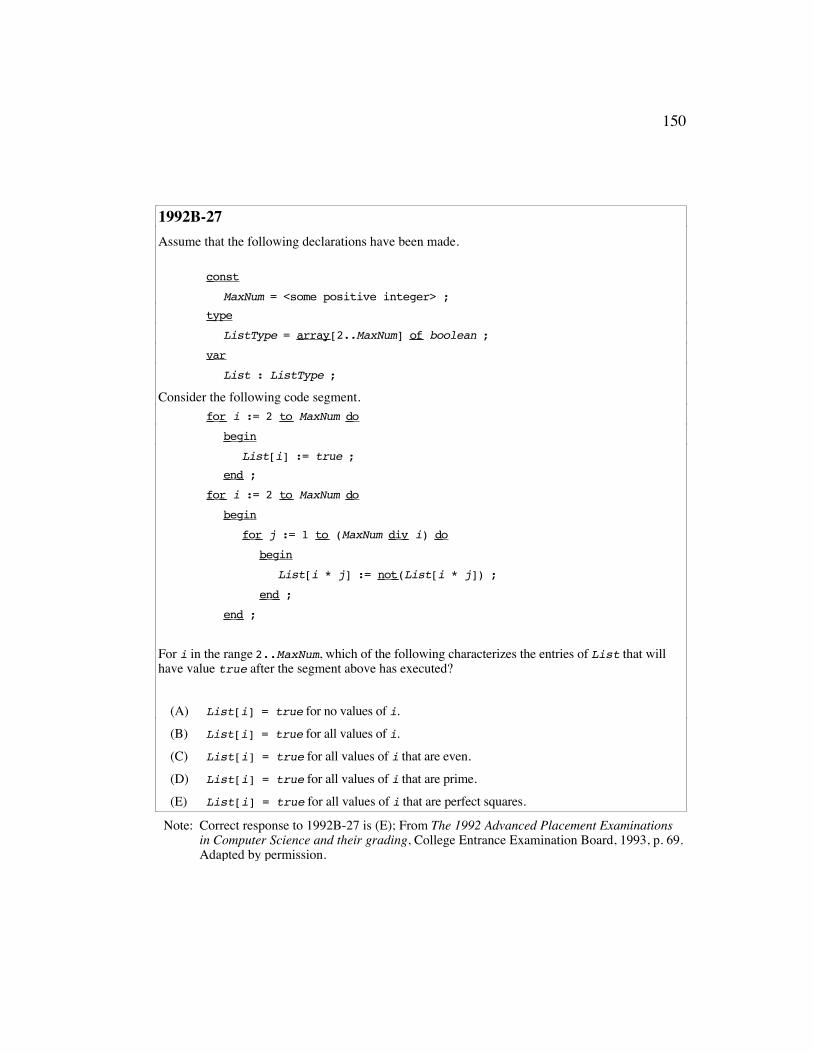
150

1992B-27Assume that the following declarations have been made.

const

MaxNum = <some positive integer> ; type

ListType = array [2..MaxNum] of boolean ;

var

List : ListType ;

Consider the following code segment. for i := 2 to MaxNum do

begin

List[i] := true ; end ;

for i := 2 to MaxNum do

begin

for j := 1 to (MaxNum div i) do

begin

List[i * j] := not (List[i * j]) ;

end ;

end ;

For i in the range 2..MaxNum, which of the following characterizes the entries of List that willhave value true after the segment above has executed?

(A) List[i] = true for no values of i.(B) List[i] = true for all values of i.(C) List[i] = true for all values of i that are even.(D) List[i] = true for all values of i that are prime.(E) List[i] = true for all values of i that are perfect squares.

Note: Correct response to 1992B-27 is (E); From The 1992 Advanced Placement Examinationsin Computer Science and their grading, College Entrance Examination Board, 1993, p. 69.Adapted by permission.

151

1992B-31&32are based on the following code framework.

var

n,i,v : integer ; begin

read(n) ;i := 1 ;v := 1 ; while <condition> do

begin

<body> ; end ;

writeln(v) ; end ;

The placeholders <condition> and <body> are to be replaced with code so that whenever thevalue read into variable n is positive, the value output is n! (n factorial). Further, the expressionv#=#i! is to be maintained as an invariant of the while loop.

1992B-31Which of the following choices for <body> maintains v = i! as the loop invariant?

(A) i := i + 1 ; v := v * i

(B) v := v * i ; i := i + 1

(C) i := i + 1 ; v := n * i

(D) v := n * i ; i := i + 1

(E) i := i * (i - 1) ; v := v + 1

1992B-32Assume that <body> has been replaced with code that maintains v = i! as the loop invariant.Which of the following choices for <condition> ensures that if the loop terminates, the value n!is output?

(A) i = n

(B) i <> n

(C) i = v

(D) i <> v

(E) i = v * n

Note: Correct responses to 1992B-31 and 1992B-32 are (A) and (B), respectively; From The1992 Advanced Placement Examinations in Computer Science and their grading, CollegeEntrance Examination Board, 1993, p. 73. Adapted by permission.

152

1992A-26 and1992B-16

Under which of the following conditions must the following boolean expression have the valuetrue ?

((i <= n) and (a[i] = 0)) or ((i >= n) and (a[i - 1] = 0))

(A) (i <= n) or (i >= n)

(B) (a[i] = 0) and (a[i - 1] = 0)

(C) i = n

(D) i < n

(E) i > n

Note: Correct response to 1992A-26/1992B-16 is (B); From The 1992 Advanced PlacementExaminations in Computer Science and their grading, College Entrance ExaminationBoard, 1993, pp. 27 & 63. Adapted by permission.

1992A-27 and1992B-17

Evaluation of the boolean expression((i <= n) and (a[i] = 0)) or ((i >= n) and (a[i - 1] = 0))

is guaranteed to cause a run-time error under which of the following conditions?

(A) i < 0

(B) Neither a[i] nor a[i - 1] has the value zero.(C) Array a is of size n.(D) Array a is of size 2.(E) None of the above

Note: Correct response to 1992A-27/1992B-17 is (E); From The 1992 Advanced PlacementExaminations in Computer Science and their grading, College Entrance ExaminationBoard, 1993, pp. 27 & 63. Adapted by permission.

153

154

1992A-31 and1992B-18

Consider the following declarations. type

ListType = record

Items : array [1..MaxLength] of integer;

NumItems : integer ; end ;

procedure Find(List : ListType ; Num : integer ;

var Found : boolean ; var Loc : integer) ;

{precondition: 0 ≤ List.NumItems ≤ MaxLength} begin

Found := false ;Loc := 0; while not Found and (Loc < List.NumItems) do

begin

Loc := Loc + 1 ; if List.Items[Loc] = Num then

Found := true ; end ;

end ;

Which of the following is a correct postcondition for procedure Find?

(A) Found

(B) Found and (Loc >= List.NumItems)

(C) (List.Items[Loc] = Num) or (Loc = List.NumItems)

(D) Loc = List.NumItems

(E) not Found and (Loc < List.NumItems)

Note: Correct response to 1992A-31/1992B-18 is (C); From The 1992 Advanced PlacementExaminations in Computer Science and their grading, College Entrance ExaminationBoard, 1993, pp. 31 & 64. Adapted by permission.

155

1992A-32 and1992B-21

The boolean expression(Num > Max) or not (Max < Num)

can be simplified to

(A) Max <> Num

(B) Max = Num

(C) (Num < Max) and not (Max < Num)

(D) false

(E) true

Note: Correct response to 1992A-32/1992B-21 is (E); From The 1992 Advanced PlacementExaminations in Computer Science and their grading, College Entrance ExaminationBoard, 1993, pp. 32 & 66. Adapted by permission.

156

Appendix H Reliability of Individual Judges

Appendix H provides an overview of the reliability of individual judges

during the final phase of the content analysis procedure. Figures H.1 through H.4

present graphs that show the reliability of each judge on the 1984, 1988, 1992

version A, and 1992 version AB examination packets respectively. Judge

numbering across the examinations is consistent, that is, judge number x on the

1984 examination is also judge number x on the 1988 and 1992 examinations.

Individual judge reliability indicates the extent to which an individual

judge was the source of unreliable data (Krippendorff, 1980). Each graph shows

the overall reliability values under the liberal and conservative partitioning

algorithms (graphed as horizontal lines), individual judge reliability under the

liberal algorithm (graphed as a black diamond), and individual judge reliability

under the conservative algorithm (graphed as a white circle). In this study,

individual judge reliability was calculated based on the test-test condition by

which the ratings were generated. In a test-test situation, the reliability of

particular individual is calculated by comparing the outcome of that individual’s

ratings of the items to the pooled ratings by all of the other judges. (This is in

contrast to a test-standard condition, where a judge’s rating performance during a

training session would be compared to a pre-existing standard. The test-standard

condition could be used for the purpose of identifying highly capable judges and

for eliminating inconsistent judges, important issues when accuracy is a key goal

of the content analysis procedure.)

157

Figure H.1, which reports judge reliability on the 1984 examination,

includes two judges, #24 and #26, whose agreement coefficients differed

drastically from those of the other judges. Under the conservative partitioning

algorithm, these two judges’ reliability was –.30 to –.40, indicating a fairly

systematic deviation from the classifications assigned by the other 36 judges. In

1988 (see Figure H.2), the reliability of judge #26 was still rather different than

the reliability of the remaining judges, particularly under the conservative

partitioning algorithm. On the 1992 examinations (see Figures H.3 and H.4), the

reliability of judge #26 was comparatively low on the A version but nearer that of

other judges on the AB version.

In 1984 as well as in other years, several other judges consistently had

lower reliability than the others (although they differed less radically than the

judges in the previous paragraph). For example, the reliability of judge #9

hovered at about .25 for the liberal partitioning algorithm on the 1984, 1988, and

1992A examinations and increased to about .40 for the 1992AB examination.

Individual reliability for judge #34 was about the same as the individual reliability

of the other judges in 1984 and 1988 but, for both versions of the 1992

examination, was lowest under the liberal partitioning algorithm and among the

lowest under the conservative partitioning algorithm.

158

liberal algorithmconservative algorithmliberal algorithmconservative algorithm

Reliability of judge compared to rest:

Overall reliability:

judge number

-0.50

-0.25

0.00

0.25

0.50

0.75

1.00

1 2 3 4 5 6 7 8 9 10 11 12 13 14 15 16 17 18 19 20 21 22 23 24 25 26 27 28 29 30 31 32 33 34 35 36 37 38

(number of judges = 38)

Figure H.1 Comparison of Agreement Coefficients of Individual Judges onExamination Packet for 1984 under Liberal and Conservative PartitioningAlgorithms

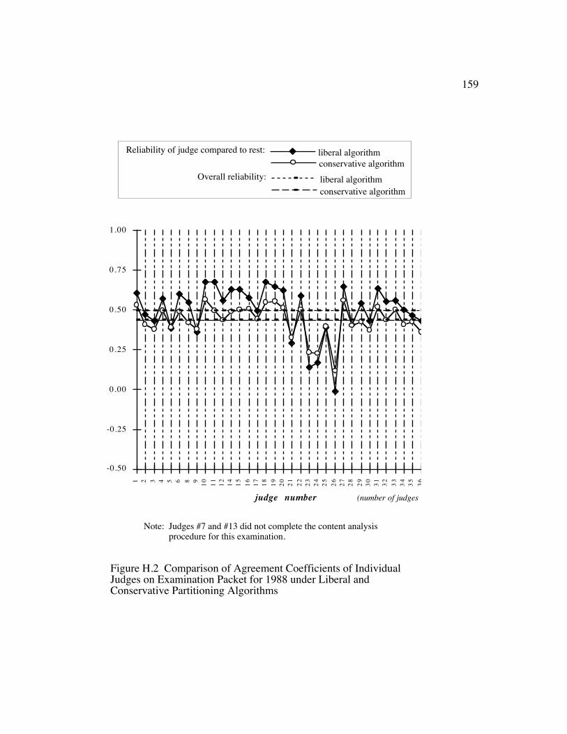
159

liberal algorithmconservative algorithmliberal algorithmconservative algorithm

Reliability of judge compared to rest:

Overall reliability:

judge number

-0.50

-0.25

0.00

0.25

0.50

0.75

1.00

1 2 3 4 5 6 8 9 10 11 12 14 15 16 17 18 19 20 21 22 23 24 25 26 27 28 29 30 31 32 33 34 35 36 37 38

(number of judges = 36)

Note: Judges #7 and #13 did not complete the content analysisprocedure for this examination.

Figure H.2 Comparison of Agreement Coefficients of IndividualJudges on Examination Packet for 1988 under Liberal andConservative Partitioning Algorithms

160

liberal algorithmconservative algorithmliberal algorithmconservative algorithm

Reliability of judge compared to rest:

Overall reliability:

judge number

-0.50

-0.25

0.00

0.25

0.50

0.75

1.00

1 2 3 4 5 6 7 8 9 10 11 12 13 14 15 16 17 18 19 20 21 22 23 24 25 26 27 28 29 30 31 32 33 34 35 36 37 38

(number of judges = 38)

Figure H.3 Comparison of Agreement Coefficients of IndividualJudges on Examination Packet for Version A of 1992 Examinationunder Liberal and Conservative Partitioning Algorithms

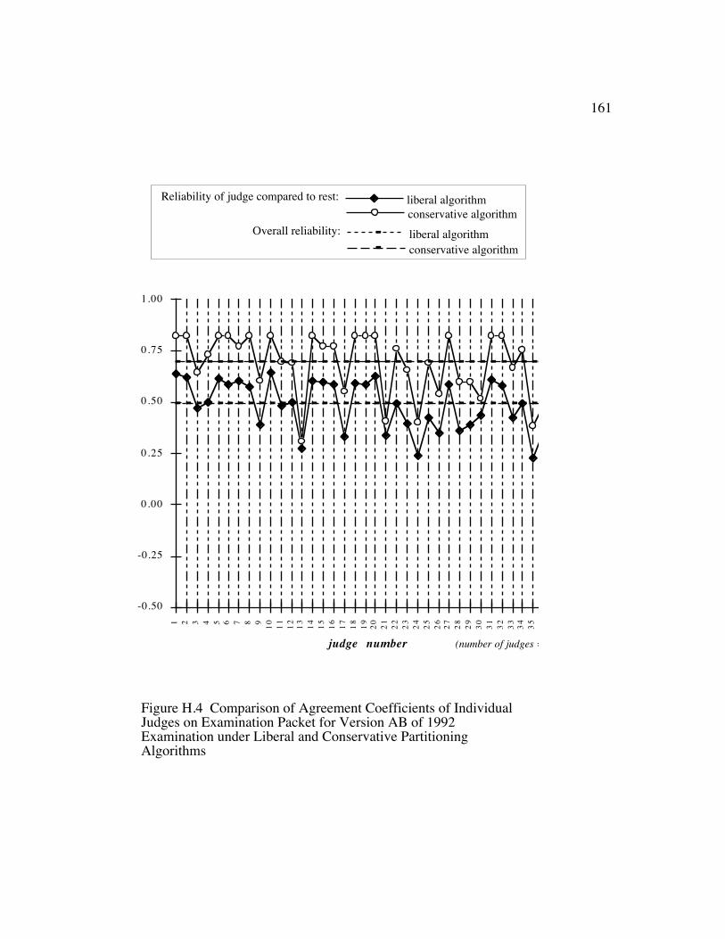
161

liberal algorithmconservative algorithmliberal algorithmconservative algorithm

Reliability of judge compared to rest:

Overall reliability:

judge number

-0.50

-0.25

0.00

0.25

0.50

0.75

1.00

1 2 3 4 5 6 7 8 9 10 11 12 13 14 15 16 17 18 19 20 21 22 23 24 25 26 27 28 29 30 31 32 33 34 35 36 37 38

(number of judges = 38)

Figure H.4 Comparison of Agreement Coefficients of IndividualJudges on Examination Packet for Version AB of 1992Examination under Liberal and Conservative PartitioningAlgorithms

162

Appendix I Rating Comparison for Duplicate Items on the A andAB Versions of the 1992 APCS Examination

Appendix I compares the judging results for the 15 items that appeared on

both the A and AB versions of the 1992 APCS examination. The results for the

duplicate items are considered in terms of the paired ratings from each judge for

the A and AB versions of the examination packets. A rating pair is expressed as

the pair of categories (pij , qij), where pij is the rating given by judge i to duplicate

item j on the one version of the examination and qij is the rating given by judge i

to duplicate item j on the other version of the examination. The item numbering

corresponds to that given in Table 4.9. In doing the content analysis, the judge

was free to complete the examination packets in any order. As a result, each

rating pair is unordered with respect to the two versions of the examination.

Instead, differences in ratings will be ordered by the categories ‘main concept’,

‘vital subconcept’, ‘trivial subconcept’, and ‘not used’ without regard to the

version for which the rating was given.

For every rating pair, either

pij = qij (the judge gave the same rating to the item on both versions of the

examination), or

pij ≠ qij (the judge gave different ratings to the item on the two versions of the

examination).

Tables I.1 and I.2 are 15X2 tables, with one row for each duplicate item.

Each entry in Table I.1 is the number of judges for whom pij = qij, while each

163

entry in Table I.2 is the number of judges for whom pij ≠ qij. (For both Table I.1

and Table I.2, he sum of the row marginals is 15, the number of duplicate items.)

Tables I.3 and I.4 are 38X2 tables, with one row for each individual judge.

Each entry in Table I.3 shows the number of items for which pij = qij , while each

entry in Table I.4 shows the numbers of items for which pij ≠ qij. (For both Table

I.3 and Table I.4, the sum of the row marginals in is 38, the number of judges who

rated the items.)

In all of the tables, the column marginals for the consistently-rated items

are much higher than the column marginals for the inconsistently-rated items.

(The consistently-rated items are those in Tables I.1 and I.3, where pij = qij; the

inconsistently-rated items are those in Tables I.2 and I.4, where pij ≠ q ij.) In

considering the all ratings pairs with pij ≠ qij, four classes of mismatches emerge:

• The rating pair was either (‘main concept’, ‘vital subconcept’) or (‘trivial

subconcept’, ‘not used’). Since these combinations did not affect the

pooling of the categories into the dichotomous scale of not strongly

related and strongly related, they did not affect the outcome.

• The rating pair was (‘vital subconcept’, ‘trivial subconcept’). This

combination straddled the dividing line between the dichotomous

categories not strongly related and strongly related, so complicated the

process of simplifying the data.

• The rating pair was either (‘vital subconcept’, ‘not used’) or (‘main

concept’, ‘trivial subconcept’). This combination was a more extreme

version of the second class of mismatch, since these combinations could

164

be considered to have a greater “distance” between them, thus making the

process of simplifying the data more complicated.

• The rating pair was (‘main concept’, ‘not used’). Since this pairing

represents a complete change of opinion, this rating mismatch is the most

troublesome.

In the final content analysis results, 76% of the rating pairs were

consistent. Of the remaining 24% of the ratings pairs, 53% fell into the first class

of rating mismatch, 21% fell into the second class of rating mismatch, 22% fell

into the third class of rating mismatch, and only 4% fell into the fourth class of

rating mismatch. (These figures represent 13%, 5%, 5%, and 1% of the total

number of ratings pairs respectively.)

165

Table I.1 Number of Judges Giving Same Rating to Duplicate Items in theContent Analysis of the A and AB Versions of the 1992 APCS Examination

rating on A /AB version of 1992 examinationitem numbers main / main vs / vs triv / triv nu / nu totals:

92A-02 / 92B-02 0 3 11 22 3692A-05 / 92B-05 2 6 16 5 2992A-07 / 92B-07 0 1 2 35 3892A-08 / 92B-04 8 11 6 2 2792A-09 / 92B-09 0 10 18 1 2992A-10 / 92B-10 0 12 17 2 3192A-16 / 92B-16 10 0 0 0 1092A-17 / 92B-17 1 1 0 0 292A-20 / 92B-06 9 12 7 0 2892A-28 / 92B-28 1 1 5 26 3392A-29 / 92B-29 2 10 15 5 3292A-31 / 92B-18 25 7 0 0 3292A-32 / 92B-21 38 0 0 0 3892A-37 / 92B-37 0 1 5 28 3492A-38 / 92B-38 0 1 5 28 34

totals: 96 76 107 154 433Note: main is ‘main concept’; vs is ‘vital subconcept’;

triv is ‘trivial subconcept’; nu is ‘not used’

166

Table I.2 Number of Judges Giving Different Ratings to Duplicate Items in theContent Analysis of the A and AB Versions of the 1992 APCS Examination

rating on A /AB version of 1992 examinationitem numbers main / vs triv / nu vs / triv main / triv vs / nu main / nu totals:

92A-02 / 92B-02 0 1 1 0 0 0 292A-05 / 92B-05 2 5 1 0 1 0 992A-07 / 92B-07 0 0 0 0 0 0 092A-08 / 92B-04 7 2 2 0 0 0 1192A-09 / 92B-09 1 3 4 0 1 0 992A-10 / 92B-10 0 3 2 0 2 0 792A-16 / 92B-16 17 0 0 8 0 3 2892A-17 / 92B-17 14 1 5 14 0 2 3692A-20 / 92B-06 3 1 5 1 0 0 1092A-28 / 92B-28 0 3 2 0 0 0 592A-29 / 92B-29 0 1 4 0 1 0 692A-31 / 92B-18 4 0 1 0 0 1 692A-32 / 92B-21 0 0 0 0 0 0 092A-37 / 92B-37 0 2 1 0 1 0 492A-38 / 92B-38 0 2 1 0 1 0 4

totals: 48 24 29 23 7 6 137Note: main is ‘main concept’; vs is ‘vital subconcept’;

triv is ‘trivial subconcept’; nu is ‘not used’

167

Table I.3 Number of Duplicate Items Given Same Rating in the Content Analysisof the A and AB Versions of the 1992 APCS Examination

rating on A /AB version of 1992 examinationmain / main vs / vs triv / triv nu / nu totals:

Judge #1 5 0 4 5 14Judge #2 1 1 2 3 7Judge #3 1 3 0 7 11Judge #4 2 4 2 5 13Judge #5 3 2 0 5 10Judge #6 1 2 7 1 11Judge #7 2 1 0 5 8Judge #8 1 1 6 5 13Judge #9 4 5 0 2 11

Judge #10 2 0 3 4 9Judge #11 2 0 0 5 7Judge #12 1 1 3 7 12Judge #13 5 1 3 0 9Judge #14 2 1 3 6 12Judge #15 2 2 4 5 13Judge #16 4 0 3 6 13Judge #17 6 3 0 5 14Judge #18 2 0 3 6 11Judge #19 1 2 3 6 12Judge #20 2 1 4 4 11Judge #21 2 1 4 4 11Judge #22 3 5 1 4 13Judge #23 4 4 3 3 14Judge #24 4 1 3 1 9Judge #25 7 3 3 1 14Judge #26 1 8 3 1 13Judge #27 1 3 0 5 9Judge #28 1 9 0 4 14Judge #29 1 3 2 4 10Judge #30 2 0 6 3 11Judge #31 2 1 7 3 13Judge #32 2 0 6 5 13Judge #33 3 4 2 5 14

Table continued on following page

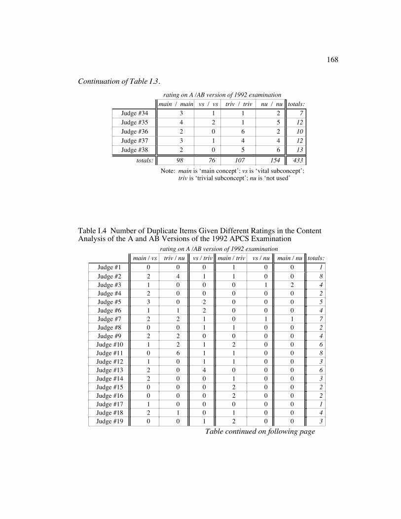
168

Continuation of Table I.3.rating on A /AB version of 1992 examination

main / main vs / vs triv / triv nu / nu totals:Judge #34 3 1 1 2 7Judge #35 4 2 1 5 12Judge #36 2 0 6 2 10Judge #37 3 1 4 4 12Judge #38 2 0 5 6 13

totals: 98 76 107 154 433Note: main is ‘main concept’; vs is ‘vital subconcept’;

triv is ‘trivial subconcept’; nu is ‘not used’

Table I.4 Number of Duplicate Items Given Different Ratings in the ContentAnalysis of the A and AB Versions of the 1992 APCS Examination

rating on A /AB version of 1992 examinationmain / vs triv / nu vs / triv main / triv vs / nu main / nu totals:

Judge #1 0 0 0 1 0 0 1Judge #2 2 4 1 1 0 0 8Judge #3 1 0 0 0 1 2 4Judge #4 2 0 0 0 0 0 2Judge #5 3 0 2 0 0 0 5Judge #6 1 1 2 0 0 0 4Judge #7 2 2 1 0 1 1 7Judge #8 0 0 1 1 0 0 2Judge #9 2 2 0 0 0 0 4Judge #10 1 2 1 2 0 0 6Judge #11 0 6 1 1 0 0 8Judge #12 1 0 1 1 0 0 3Judge #13 2 0 4 0 0 0 6Judge #14 2 0 0 1 0 0 3Judge #15 0 0 0 2 0 0 2Judge #16 0 0 0 2 0 0 2Judge #17 1 0 0 0 0 0 1Judge #18 2 1 0 1 0 0 4Judge #19 0 0 1 2 0 0 3

Table continued on following page

169

Continuation of Table I.4.rating on A /AB version of 1992 examination

main / vs triv / nu vs / triv main / triv vs / nu main / nu totals:Judge #20 1 1 2 0 0 0 4Judge #21 1 0 0 1 2 0 4Judge #22 2 0 0 0 0 0 2Judge #23 1 0 0 0 0 0 1Judge #24 3 0 2 0 0 1 6Judge #25 1 0 0 0 0 0 1Judge #26 1 0 0 1 0 0 2Judge #27 4 1 1 0 0 0 6Judge #28 1 0 0 0 0 0 1Judge #29 2 1 2 0 0 0 5Judge #30 3 0 1 0 0 0 4Judge #31 1 0 0 1 0 0 2Judge #32 1 0 0 1 0 0 2Judge #33 1 0 0 0 0 0 1Judge #34 2 2 1 0 3 0 8Judge #35 1 0 1 1 0 0 3Judge #36 0 0 3 2 0 0 5Judge #37 0 1 1 0 0 1 3Judge #38 0 0 0 1 0 1 2

totals: 45 24 29 24 7 6 137Note: main is ‘main concept’; vs is ‘vital subconcept’;

triv is ‘trivial subconcept’; nu is ‘not used’

170

Glossary

abstract datatype: A datatype described only at the logical level, without detailsof implementation.

ACM: The Association for Computing Machinery, one of the key professionalorganizations in the field of computer science. Provides a variety offorums for the dissemination of technical information and discussions ofissues important to the computing profession.

APCS : Advanced Placement Computer Science, one of the subject-areaexaminations offered annually by ETS to high school students.

ASL: The Association for Symbolic Logic, a worldwide organization dedicatedto the study of logic.

assertion: A predicate within the context of a program. The predicate assertswhat must true about the program state at that point.

boolean: An abstract datatype that is based on the set of values {true, false}7.The operations are the logical connectives.

boolean expression: An expression constructed from boolean constants, booleanvariables, boolean operations, and operations from other domains whoseresult type is boolean (e.g., 9"+"3"="12, 7"<"4, ax"+"by"≠"c, ‘xy’"<"’xyz’). 8

classical logic: A branch of logic that assumes that the values true and false forma dichotomy, so that anything that is not true is false and vice versa.

constant: A computational object associated with a particular datatype; has anunchanging and unchangeable value from the datatype domain.

content analysis: A research technique for making replicable and validinferences from data to their context.

data object: A variable or constant; defined by means of a datatype.

data structure: Representation of a data object within a computer program. 7 Because these values are part of a set, the values of type boolean considered in “pure” form

are unordered. However, some programming languages impose an artificial ordering on thesevalues. In Pascal, for example, boolean is implicitly defined by the declaration

type boolean = (false, true)which defines false < true to be valid.

8 Note that, while the expression 7 < 4 evaluates to “false”, it is still a valid boolean expression.

171

data type: See datatype.

datatype: The formal description of the characteristics of a group of related dataobjects; includes a domain (or set of distinct values), a collection ofrelationships among the values of the domain, and a set of operations onthe values.9

ETS: Educational Testing Service, the organization that provides the operationalservices for the College Entrance Examination Board. Responsible for theAdvanced Placement Program and the Graduate Record ExaminationProgram, as well as other programs.

identifier: A sequence of one or more digits and letters; the name of a dataobject, datatype, proposition, or predicate.

IEEE: The Institute of Electronics and Electrical Engineers; has as its purpose toadvance the theory and practice of computer science and engineering andto promote the exchange of technical information.

ISO: International Standards Organisation.

logic: A science that deals with the rules and criteria of valid inference anddemonstration; the science of the formal principles of reasoning.

logical connectives: Operators defined over values of type boolean; includenegation (“not” or ÿ), conjunction (“and” or Ÿ), disjunction (“or” or ⁄),implication (“implies” or fi ), and equality (“equals” or = ; also“equavales” or ≡).

LID: Language-Independent Datatype, the topic of an ISO standard (1994).

MAA: Mathematical Association of America.

mathematical logic: A branch of logic that uses a formalized system consistingof primitive symbols, combinations of these symbols, axioms, and rules ofinference. Also called symbolic logic, logistic.

9 Whether datatype is one word or two is an unresolved issue. B. Meeks has argued that the

one-word spelling conveys that this is a “reserved word” denoting a specific concept, not tobe confused with other notions of “types” of data. The translation into French of “data type”was established as “type des donne’s”, literally the “type of the data”, which could beinterpreted in many ways, whereas the translation of “datatype” would be “type de donne’s”— the “type of data”, which implied reference to some specific system of categories. A quicksurvey of programming language standards revealed that only Fortran refers to “data type”and only Prolog uses “datatype”. COBOL refers to “classes of data”. The Ada, Pascal,C/C++, and SmallTalk standards refer only to “type”. (E. Barkmeyer, personalcommunication, April 12, 1994)

172

operator: A mathematical or logical symbol denoting an operation to beperformed.

postcondition: The assertion that is the second half of the specification of asequential program or statement; specifies that which must hold after theprogram or statement is executed.

precondition: The assertion that is the first half of the specification of asequential program or statement; specifies that which must hold before theprogram or statement is executed.

predicate: A formula of the predicate calculus.

predicate calculus: The branch of mathematical logic that uses symbols forquantifiers and for arguments and predicates of propositions as well as forunanalyzed propositions and logical connectives; also called functionalcalculus.

program space: The set of data objects that are defined at a particular timeduring execution of a computer program.

program state: The values of the data objects in the program space at aparticular time during execution of a computer program.

proposition: An expression in language or signs of something that can bebelieved, doubted, or denied or is either true or false. A symbolicproposition is formed according to the following rules: (1) true and falseare propositions; (2) an identifier is a proposition; (3) if b is aproposition, then so is ÿb; and (4) if b and c are propositions, then so are(a Ÿ b), (a ⁄ b), (a fi b), and (a ≡ b).

propositional calculus: The branch of mathematical logic that uses symbols forunanalyzed propositions and logical connectives only; also calledsentential calculus.

PLT: Propositional Logic Test.

specification: A formal description of the desired behavior of a computerprogram or other code fragment. In sequential programs, the specificationconsists of a pair of assertions, the precondition and the postcondition.

two-valued logic: Propositional logic specifically restricted to a domain of twovalues.

type: A synonym for “datatype” when used in the context of describing a dataobject.

173

variable: A computational object associated with a particular datatype; has aspecific value from the datatype domain at any given time and may havedifferent values of the same domain at different times.

Credits:

• The data-related definitions were influenced by Dale & Walker (in press).

• The calculus and boolean definitions have been influenced by Gries (1981),ISO (1994), and Tucker, Bradley, Cupper, & Garnick (1992).

• The logic definitions have been influenced by Cumbee (1993) & Webster(1972).

• The definition of content analysis is based on Krippendorff (1980, p. 21).

• The definition of operator is suggested by Webster (1972).

174

Bibliography

Anderson, J. R. (1980). Cognitive Psychology and its implications. SanFrancisco: W. H. Freeman.

ASL. (in press). Association of Symbolic Logic Guidelines for Logic Education.Bulletin of Symbolic Logic.

Atchison, W. F. (chair). (1968). Curriculum '68: Recommendations foracademic programs in computer science. Communications of the ACM,11(3), 151–197.

Austing, R. H. (chair). (1979). Curriculum '78: Recommendation for theundergraduate program in computer science. Communications of theACM, 22(3), 147–166.

Baker, D., & VanHarlingen, D. (1979, March). The relationship of Piagetian andPiagetian-like tasks to physics achievement. Paper presented at themeeting of the National Association for Research in Science Teaching,Atlanta, GA (abs.).

Belnap, N. D, Jr., & Grover, D. L. (1973). Quantifying in and out of quotes. InH. Leblanc (Ed.), Truth, syntax and modality: Proceedings of the TempleUniversity Conference on Alternative Semantics (pp. 17–47). Amsterdam:North-Holland.

Bennett, R. E., Rock, D. A., & Wang, M. (1991). Equivalence of free-responseand multiple-choice items. Journal of Educational Measurement , 28 ,77–92.

Berztiss, A. (1987). A mathematically focused curriculum for computer science.Communications of the ACM, 30(5), 356–365.

Boute, R. T. (1990). A heretical view on type embedding. SIGPLAN Notices,25(1), January. 25–28.

Boute, R. T. (1991). Letter to the Editor. SIGPLAN Notices, 26(2), February.9–10.

Church, A. (1956). Introduction to Mathematical Logic (Vol. 1). Princeton, NJ:Princeton University Press.

College Board. (1986). The Entire 1984 AP Computer Science Examination andKey. College Entrance Examination Board.

175

College Board. (1989). The 1988 Advanced Placement Examinations inComputer Science and their grading. College Entrance ExaminationBoard.

College Board. (1990). Advanced Placement Course Description: ComputerScience. College Entrance Examination Board. May 1991 version.

College Board. (1993). The 1992 Advanced Placement Examinations inComputer Science and their grading. College Entrance ExaminationBoard.

Cooke, J. (1992). Formal methods — mathematics, theory, recipes, or what?The Computer Journal, 35(5), 419–423.

Copi, I. M. (1979). Symbolic Logic (5th ed.). New York: Macmillan.

Cumbee, J. (1993). Mathematical logic. Academic American Encyclopedia[electronic data file from database on UTCAT PLUS system]. Danbury,CT: Grolier Electronic Publishing, September update from 1991 version.

Dale, N., & Walker, H. (in press). Abstract data types: Specification,implementation, and application. Lexington, MA: D. C. Heath.

Denning, P. J. (chair). (1989). Computing as a discipline. Communications ofthe ACM, 32(1), 9–23.

Dijkstra, E. W. (1968). A constructive approach to the problem of programcorrectness. BIT, 8, 174–186.

Dijkstra, E. W. (1976). A discipline of programming. Englewood Cliffs, NJ:Prentice-Hall.

Dijkstra, E. W. (1989). On the cruelty of really teaching computing science.Communications of the ACM, 32(12), 1398–1404.

Dijkstra, E. W., & Feijen, W. H. J. (1988). A method of programming. MenloPark, CA: Addison-Wesley.

Dijkstra, E. W., & Scholten, C. S. (1990). Predicate calculus and programsemantics. New York: Springer-Verlag.

Enyeart, M., VanHarlingen, D., & Baker, D. (1980). The correlation of inductiveand deductive reasoning to college physics achievement. Journal ofResearch in Science Teaching, 17(3), 262–267.

Evans, J. St. B. T. (1980). Current issues in the psychology of reasoning. BritishJournal of Psychology, 71, 227–239.

176

Floyd, R. W. (1967). Assigning meaning to programs. Proceedings of theAmerican Mathematical Society Symposia in Applied Mathematics, 19,19–32.

Franzblau, D. (1993). New models for courses in discrete mathematics. SIAGDM News, November 15.

Furth, H. G. (1969). Piaget and knowledge: Theoretical foundations.Englewood Cliffs, NJ.

Galton, A. (1992). Logic as a Formal Method. The Computer Journal, 35(5),431–440.

Gardner, H. (1985). Frames of mind: The theory of multiple intelligences. BasicBooks.

Gardner, H., & Hatch, T. (1989). Multiple Intelligences go to school:Educational implications of the theory of multiple intelligences.Educational Researcher, November, 4–10.

Gibbs, N. E., & Tucker, A. B. (1986). A model curriculum for a liberal artsdegree in computer science. Communications of the ACM, 29(3),202–210.

Ginsberg, H., & Opper, S. (1979). Piaget’s theory of intellectual development(2nd ed.). Englewood Cliffs, NJ: Prentice-Hall.

Goldson, D., Reeves, S., & Bornat, R. (1993). A review of several programs forthe teaching of logic. The Computer Journal, 36(4), 373–386.

Gries, D. (1981). The Science of Programming. New York: Springer-Verlag.

Gries, D. (1990). Calculation and discrimination: A more effective curriculum.Communications of the ACM. 34(3). 44–55.

Gries, D., & Schneider, F. B. (1993a). A logical approach to discretemathematics. New York: Springer-Verlag.

Gries, D., & Schneider, F. B. (1993b). Instructor’s manual: A logical approachto discrete mathematics. Ithaca, NY: Computer Science Department,Cornell, University.

Gries, D., & Schneider, F. B. (1994). A new approach to teaching mathematics.Unpublished manuscript, Cornell University, Computer ScienceDepartment, Ithaca, NY.

177

Guilford, J. P. (1967). The nature of human intelligence. New York: McGraw-Hill.

Hasenjaeger, G. (1972). Introduction to the basic concepts and problems ofmodern logic. Dordrecht, Holland: D. Reidel Publishing.

Hilbert, D., & Ackermann, W. (1950). Principles of mathematical logic. NewYork: Chelsea Publishing.

Hoare, C. A. R. (1969). An axiomatic basis for computer programming.Communications of the ACM, 1 2 , 576–583. (Reprinted inCommunications of the ACM, 1983, 26(1), 53–56).

IEEE Computer Society Education Committee. (1976). A Curriculum inComputer Science and Engineering. IEEE Computer Society, ModelCurriculum Subcommittee.

IEEE Model Program Committee. (1983). The 1983 IEEE Computer SocietyModel Program in Computer Science and Engineering. IEEE ComputerSociety. Educational Activities Board.

Inhelder, B., & Piaget, J. (1958). The growth of logical thinking from childhoodto adolescence. New York: Basic Books.

Irons, E. T. (1961). A syntax directed compiler for ALGOL 60.Communications of the ACM, 4(1), 51–55.

ISO. (1994). Information technology — Language-independent datatypes.ISO/IEC draft International Standard 11404: 1994, Geneva: InternationalOrganization for Standardization.

Jensen, K., & Wirth, N. (1974). Pascal User’s Manual. New York: Springer-Verlag.

Koffman, E. B., Miller, P. L., & Wardle C. E. (1984). RecommendedCurriculum for CS1, 1984. Communications of the ACM, 27(10),998–1001.

Koffman, E. B., Stempel, D., & Wardle C. E. (1985). Recommended Curriculumfor CS2, 1984. Communications of the ACM, 28(8), 815–818.

Krippendorff, K. (1980). Content Analysis: An Introduction to Its Methodology.Beverly Hills, CA: Sage Publications.

Lefrancois, G. R. (1988). Psychology for Teaching (6th ed.). Belmont, CA:Wadsworth Publishing Company.

178

Lewis, C. I., & Langford, C. H. (1959). Symbolic Logic (2nd ed.). New York:Dover.

Lockwood, W., Pallrand, G. & VanHarlingen, D. (1980, April). The relationshipbetween logical operators and achievement in university physics. Paperpresented at the meeting of the National Association for Research inScience Teaching, Boston, MA (abs.).

Lockwood, W., Pallrand, G., & VanHarlingen, D. (1982, April). Logical abilityand achievement in high school level physics. Paper presented at themeeting of the National Association for Research in Science Teaching,Lake Geneva, WI (abs.).

Meeks, B. (1990). Two-valued datatypes. SIGPLAN Notices, 25(8) (August)75–79.

Meeks, B. (1991). Letter to the Editor. SIGPLAN Notices, 26(8), August. 24.

Merritt, S. (chair). (1993). ACM Model High School Computer ScienceCurriculum. New York: Association for Computing Machinery, TaskForce of the Pre-College Committee of the ACM Education Board.

Murfin, B. E. (1993). An Analysis of Computer-Mediated Communicationbetween Urban Middle School Students and Scientists (Urban Education)[CD-ROM]. Abstract on ProQuest: Dissertation Abstracts On Disc,January, 1993 – February 1994. Available: UMI, Order No. AAC9325561. (Doctoral Dissertation, Ohio State University; reference toDissertation Abstracts International, 5405A, p. 1770, Nov. 1993).

Myers, Jr., J. P. (1990). The central role of mathematical logic in computerscience. SIGCSE Bulletin, 22(1), 22–26.

Nocolescu, R. (1991). Letter to the Editor. SIGPLAN Notices, 26(2), February.9–10.

Pallrand, G., & VanHarlingen, D. (1980, April). Cognitive structures andachievement in physics. Paper presented at the meeting of the NationalAssociation for Research in Science Teaching, Boston, MA (abs.)

Parsons, A. (1958). Translator’s introduction: A guide for psychologists. In B.Inhelder & J. Piaget, The growth of logical thinking from childhood toadolescence, New York: Basic Books.

Petrushka, D. (1984). A study of the effect of content on the ability to dosyllogistic reasoning: An investigation of transferability and the effect ofpractice. Unpublished doctoral dissertation, Rutgers University, NJ.

179

Piburn, M. D. (1989). Reliability and validity of the Propositional Logic Test.Educational and Psychological Measurement, 49, 667–672.

Piburn, M. D. (1990). Reasoning about logical propositions and success inscience. Journal of Research in Science Teaching, 27(9), 887-900.

Piburn, M. D., & Baker, D. (1988, April). Reasoning about logical propositionsand success in science. Paper presented at the meeting of the AmericanEducational Research Association, New Orleans, LA.

PLT Key. (1989). Key to the Propositional Logic Test. Unpublished document.Obtained through M. Piburn, Arizona State University.

Pollack, S. V. (Ed.). (1982a) Studies in Computer Science. The MathematicalAssociation of America.

Pollack, S. V. (1982b). The development of computer science. In S. V. Pollack(ed.), Studies in Computer Science, The Mathematical Association ofAmerica.

Popkin, R. H. (1993a). Philosophy. Academic American Encyclopedia[electronic data file from database on UTCAT PLUS system]. Danbury,CT: Grolier Electronic Publishing, December update; copyright 1991.

Popkin, R. H. (1993b). Traditional logic. Academic American Encyclopedia[electronic data file from database on UTCAT PLUS system]. Danbury,CT: Grolier Electronic Publishing, September update; copyright 1991.

Powers, D. E., & Enright, M. K. (1987). Analytic reasoning skills involved ingraduate study: Perceptions of faculty in six fields. Journal of HigherEducation, 58, pp. 658-682.

ProQuest: Dissertation Abstracts On Disc [CD-ROM]. (January, 1993 –February, 1994). Available: UMI.

Proulx, V. K., & Wolf, C. E. (1993). Appendix F: Breadth approach usingapplications and programming modules. In Merritt, S. (chair), ACMModel High School Computer Science Curriculum, 1993, New York:Association for Computing Machinery, Task Force of the Pre-CollegeCommittee of the ACM Education Board.

Ralston, A. (Ed.) (1989). Discrete Mathematics in the First Two Years. MAANotes No. 15. The Mathematical Association of America.

Ralston, A., & Shaw, M. (1980). Curriculum '78 — Is computer science reallythat unmathematical? Communications of the ACM, 23(2), 67–70.

180

Romberg, T. A. (1989) Curriculum and Evaluation Standards for SchoolMathematics. National Council of Teachers of Mathematics

Rothaug, W. (1984). Logical connectives and community college science courseachievement. Unpublished doctoral dissertation, Rutgers University, NJ.

Rothaug, W., & Pallrand, G. (1982, April). Reasoning skills and science courseachievement. Paper presented at the meeting of the National Associationfor Research in Science Teaching, Lake Geneva, WI (abs.)

Rothaug, W., Pallrand, G., & VanHarlingen, D. (1981, April). Logicaloperations and achievement in community college students. Paperpresented at the meeting of the National Association for Research inScience Teaching, Grossingers, NY (abs.)

Saiedian, H. (1992). Mathematics of computing. Computer Science Education,3(3), 203-221.

Sakkinen, M. (1990). On embedding Boolean as a subtype of Integer. SIGPLANNotices, 25(7), 95–96.

Seeber, F., Pallrand, G., VandenBerg, G., & VanHarlingen, D. (1979, April).Logical ability, formal thought and achievement in physics. Paperpresented at the meeting of the National Association for Research inScience Teaching, Atlanta, GA (abs.)

Shaw, M. (Ed.). (1985). The Carnegie-Mellon Curriculum for UndergraduateComputer Science. New York: Springer-Verlag.

Siegel, M. (1989a). Afterthoughts: Discrete Mathematics in the First TwoYears. In A. Ralston (ed.), Discrete Mathematics in the First Two Years,MAA Notes No. 15, The Mathematical Association of America.

Siegel, M. (1989b). Final report of the MAA committee on discrete mathematicsin the first two years. In A. Ralston (ed.), Discrete Mathematics in theFirst Two Years, MAA Notes No. 15, The Mathematical Association ofAmerica.

Sperschneider, V., & Antoniou, G. (1991). Logic: A foundation for computerscience. International Computer Science Series. Reading, MA: Addison-Wesley.

Spresser, D. M., and LePera, T. (1992). Comparative review of 10 discretemathematics textbooks. Computing Reviews, February, 100–108.

Stager-Snow, D. (1985). Analytical ability, logical reasoning and attitude aspredictors of success in an introductory course in computer science for

181

non-computer science majors. (Doctoral dissertation, Rutgers University,NJ). Dissertation Abstracts International, 45, 08A, p. 2473, February,1985.

Stofflett, R. T., & Baker, D. R. (1992). The effects of training in combinatorialreasoning and propositional logic on formal reasoning ability in highschool students. Research in Middle Level Education, 16(1), 159–177.

Stolyar, A. A. (1970). Introduction to elementary mathematical logic.Cambridge, MA: MIT Press.

Stone, P. J., Dunphy, D., Smith, M. S., & Ogilvie, D. M. (1966). The GeneralInquirer: A Computer Approach to Content Analysis. Cambridge, MA:The M.I.T. Press.

Tobin, K. G., and Capie, W. (1981). The development and validation of a grouptest of logical thinking. Educational and Psychological Measurement, 41,413–423.

Tucker, A. B. (Ed.) (1990). Computing Curricula 1991: Report of theACM/IEEE-CS Joint Curriculum Task Force. Final Draft, December 17.ACM Order Number 201910. IEEE Computer Society Press OrderNumber 2220.

Tucker, A. B., Bradley, W. J., Cupper, R. D., & Garnick, D. K. (1992).Fundamentals of Computing I. New York: McGraw-Hill.

Warford, J. S. (in press). Book review of A Logical Approach to Discrete Math(1993) by D. Gries and F. B. Schneider. Computing Reviews.

Webster’s Seventh New Collegiate Dictionary . (1972). Springfield, MA: G. &C. Merriam Co.

Whitehead, A. N. (1911). An Introduction to Mathematics. Oxford, England:Oxford University Press. (From I. M. Copi, 1979, Symbolic Logic, 5thed., New York: Macmillan)

Wickens, T. D. (1989). Multiway contingency tables analysis for the socialsciences. Hillsdale, NJ: Lawrence Erlbaum Associates.

Wing, J. M. (1990). A specifier’s introduction to formal methods. Computer,23(9), 8–24.

Wirth, N. (1976). Algorithms + Data Structures = Programs. Englewood Cliffs,NJ: Prentice-Hall.

182

Vita

Vicki Lynn Almstrum was born February 13, 1955, in Tilden, Nebraska,

the daughter of Billy Harrison Almstrum and Lucille Alice Oman Almstrum. She

graduated Cum Laude from Arizona State University with a Bachelor of Arts in

Education degree, emphasis secondary education, in December, 1977, with a

major in mathematics and a minor in German. She continued her studies at

Arizona State University, receiving the Master of Arts degree in May, 1980, with

a major in mathematics and a minor in computer science. From 1980 to 1984 she

worked as a computer scientist at Motorola, Inc. in Tempe, Arizona. In 1984, she

moved to Järfälla, Sweden where she worked as a computer scientist for Philips

Electronics until 1988. On her return to the United States, she began her graduate

studies in the Department of Computer Sciences at the University of Texas at

Austin. She received the Master of Science in Computer Sciences degree in

December, 1990, and was admitted to candidacy in the doctoral program of

Mathematics Education in March, 1991, specializing in computer science

education. While pursuing her graduate work, both at Arizona State University

and the University of Texas at Austin, she worked as a teaching assistant for

undergraduate mathematics and computing science classes. She is a member of

the Association for Computing Machinery, the ACM Special Interest Groups on

Computer Science Education (SIGCSE), Software Engineering (SIGSoft), and

Computer and Human Interaction (SIGCHI), the Institute for Electrical and

Electronics Engineers and its Computer Society, Computer Professionals for

183

Social Responsibility, and Upsilon Pi Epsilon, an honor society in Computer

Science. She is married to Torgny Stadler, with whom she enjoys travel, two-

stepping, and life’s many wonders.

Permanent address:

1412 West 39th 1/2 Street

Austin, Texas 78756

Internet address: almstrum@cs.utexas.edu

This dissertation was prepared by the author using Microsoft® Word version 5.1,

Microsoft® Excel version 4.0, Aldus® PageMaker® version 5.0, and SPSS for the

Macintosh® version 4.0.