limit order strategic placement with adverse selection ... · limit order strategic placement with...
TRANSCRIPT

Limit Order Strategic Placementwith Adverse Selection Riskand the Role of Latency.
Charles-Albert Lehalle∗ and Othmane Mounjid†
Printed the March 16, 2018
Abstract
This paper is split in three parts: first we use labelled trade data to exhibit howmarket participants accept or not transactions via limit orders as a function of liquidityimbalance; then we develop a theoretical stochastic control framework to provide detailson how one can exploit his knowledge on liquidity imbalance to control a limit order. Weemphasis the exposure to adverse selection, of paramount importance for limit orders. Fora participant buying using a limit order: if the price has chances to go down the probabilityto be filled is high but it is better to wait a little more before the trade to obtain a betterprice. In a third part we show how the added value of exploiting a knowledge on liquidityimbalance is eroded by latency: being able to predict future liquidity consuming flows isof less use if you have not enough time to cancel and reinsert your limit orders. Thereis thus a rational for market makers to be as fast as possible as a protection to adverseselection. Thanks to our optimal framework we can measure the added value of latencyto limit orders placement.
To authors’ knowledge this paper is the first to make the connection between empiricalevidences, a stochastic framework for limit orders including adverse selection, and thecost of latency. Our work is a first stone to shed light on the roles of latency and adverseselection for limit order placement, within an accurate stochastic control framework.
1 Introduction
With the electronification, fragmentation, and increase of frequency of trading, orderbook dy-namics is under scrutiny. Order flow dynamics is of paramount importance since it plays amajor role in price formation. At the smallest time scale order placements have been stud-ied as a system using economics, econophysics and applied mathematics (see [Lo et al., 2002],[Bouchaud et al., 2004], [Huang et al., 2015b] and references herein). On the one hand, at alarger time scale, investors’ decisions are split into large collections of limit (i.e. liquidity pro-viding) orders and market (i.e. liquidity consuming) orders and contribute to price formation(see [Kyle, 1985], [Toth et al., 2012], [Bacry et al., 2014] and their references for three differ-ent viewpoints on price formation and market impact). The two time scales are linked sincedynamics around small orders are shaping the market impact of the large metaorders they arepart of (see [Zarinelli et al., 2015] for a discussion about this relationship).
∗Capital Fund Management, Paris and Imperial College, London†Universite Pierre et Marie Curie, Paris
1
arX
iv:1
610.
0026
1v1
[q-
fin.
TR
] 2
Oct
201
6

On the other hand, (high frequency) market makers mostly use limit orders, providingliquidity to child orders of investors. Price dynamics around their orders have been studied too(see for instance [Biais et al., 2016] for small time scales and [van Kervel and Menkveld, 2014]for large time scales).
In practice market makers and investors use optimal trading strategies to bind the twotime scales. Models for these strategies are now well known (see [Gueant et al., 2013] and[Gueant et al., 2012] for a common framework involving limit orders for market makers andinvestors). For obvious reasons, the focus of papers about optimal trading strategies has beenrisk control. In practice market participants combine short term anticipations of price dynamicsinside these risk control framework ([Almgren and Lorenz, 2006] for the inclusion of a Bayesianestimator of the price trend in a mean-variance optimal trading strategy).
This paper focuses on the optimal control of one limit order (potentially included in anoptimal strategy at a largest time scale, see [Lehalle et al., 2013, Chapter 3] for a practitionerviewpoint on splitting the two time scales of metaorders executions) taking profit of a shortterm anticipation of price moves.
After some considerations about short time predictions in orderbooks and empirical ev-idences showing market participants take imbalance into account, we first show that in thecontext of a very simple choice (canceling or (re) inserting a limit order) optimal control canadd value to any short term predictor. This result can thus be used by investors or marketmakers to include some predictive power in their optimal trading strategies.
Then we show how latency influences the efficient use of such predictions. As expected themore latency to take decision, the less one can take profit of optimal control. It allows us tolink our work to regulatory questions. First of all: what is the “value” of latency? Regulatorscould hence rely on our results to take decisions about “slowing down” or not the market (see[Fricke and Gerig, 2014] and [Budish et al., 2015] for discussions about this topic). It shedsalso light on maker-taker fees since the real value of limit orders (including adverse selectioncosts), are of importance in this debate (see [Harris, 2013] for a discussion).
This paper can be seen as a mix of two early works presented at the “Market Microstructure:Confronting Many Viewpoints” conference (Paris, 2014): a data-driven one focused on the pre-dictive power of orderbooks [Stoıkov, 2014], and an optimal control driven one [Moallemi, 2014].Our added values are first a proper combination of the two aspects (inclusion of an imbalancesignal in an optimal control framework for limit orders), and then the construction of our costfunction. Unlike in the second work, we do not value a transaction with respect to the mid-priceat t = 0, but with respect to the microprice (i.e. the expected future price given the imbalance)at t = +∞. We will argue the difference is of paramount importance since it introduces aneffect close to adverse selection aversion, that is crucial in practice.
As an introduction of our framework, we will use a database of labelled transactions onNASDAQ OMX (Nordic European regulated markets) to show how orderbook imbalance isused by market participants in a way that can be seen as compatible with our theoreticalresults.
Hence the structure of this paper is as follows: Section 2 presents orderbook imbalance asa microprice and details our optimal control framework, and Section 3 illustrates the use ofimbalance by market participants thanks to NASDAQ OMX database. Once these elementsare in place, Section 4 presents our model and 5 shows how to numerically solve the controlproblem and provides main results, especially the influence of latency on the efficiency of thestrategy.
2

2 The Model
2.1 The Orderbook Imbalance as a Microprice
Martingality of the price changes no more stands once you add information to your knowledgeof the state of the “world” (i.e. the filtration supporting the randomness of your perception ofprice dynamics). At small time scales, well known stylized facts break the martingality of pricechanges (see [Cont, 2001] or references inside [Lehalle, 2014]) like the positive autocorrelationof the signs of trades (i.e. there is more chance the next transaction is initiated by a buyer or aseller if the previous ones have been too) and the negative autocorrelation of the returns (oncethe price moved up –respectively down– the probability it goes down –resp. up– is larger thanif the price went down –resp. up–).
When you add the state of the orderbook to your filtration, next prices moves are even“less martingale” (i.e. easier to predict). Academic papers (like [Bouchaud et al., 2004] or[Huang et al., 2015b]) and brokers’ research papers (see [Besson et al., 2016]) document howthe sizes at first limits of the public orderbook1 influences the next price change.
It is worthwhile to underline the identified effects are usually not strong enough to be thesource of a statistical arbitrage: the expected value of buying and selling back using accuratepredictions based on sizes at first limits does not beat transaction costs (bid-ask spread andfees). See [Jaisson, 2014] for a discussion. Nevertheless
• for an investor who already took the decision to buy or to sell, this information can sparesome basis points. For very large orders, it makes a lot of money and in any case itreduces implicit transaction costs.
• market makers naturally use this kind of information to add value to their trading pro-cesses (see [Fodra and Pham, 2013] for a model supporting a theoretical optimal marketmaking framework including first limit prices dynamics).
The easiest way to summarize the state of the orderbook without destroying its informationalcontent is to compute its imbalance: the quantity at the best bid minus the one at the best askdivided by the sum of these two quantities:
Imbt :=QBidt −QAsk
t
QBidt +QAsk
t
. (1)
The future price move is positively correlated with the imbalance. In other terms
E((Pt+δt − Pt)× sign(Imbt)|Imbt) > 0, (2)
where Pt is the midprice (i.e. Pt = (PBidt + PAsk)/2, where PBid and PAsk are respectively the
best bid ans ask prices) at t for any δt. Obviously when δt is very large, this expected pricemove is very difficult to distinguish from large scale sources of uncertainty. See for instance[Lipton et al., 2013] for a documentation of the “predicting power” of such an indicator (ourFigure 1 illustrates this predicting power on real data).
The nature of the predicting power of the imbalance. It is outside of the scope of thispaper to discuss and document the predicting power of the imbalance; we just give here someclues and intuitions to the reader:
1Limit orderbooks are used in electronic market to store unmatched liquidity, the bid size is the one ofpassive buyers and the ask size the one of passive sellers; see [Lehalle et al., 2013] for detailed.
3

• first of all, since the quantity at the bid is the unmatched buying quantity and the oneat the ask the unmatched selling one, it is natural to deduce at one point owners of theassociated orders will loose patience and consume liquidity, pushing the price in theirdirection.
• within a model in which market orders occurence follow independent point processes ofthe same intensity, the smallest queue (bid or ask) will be consumed first, and the pricewill be pushed in its direction. See [Huang et al., 2015b] for a more sophisticated pointprocess-driven model and associated empirical evidences.
• Another viewpoint on imbalance would be the bid vs. ask imbalance contains informationabout the direction of the net value of investors’ metaorders. Or directly (if one isconvinced investors post limit orders), or indirectly (if one believe investors only consumeliquidity and in such a case bid and ask sizes are an indicator of market makers netinventory).
The focus of definition (1) on two first limits weaken the predictive power of the bid vs. askimbalance. For large tick assets2 it may be enough to just use the first limits, but for small tickones it certainly increases the predicting power of our imbalance indicator to take more thanone tick into account. Since a discussion on the predictive power of imbalance is outside thescope of the paper, we will stop here the discussion.
This paper is providing a stochastic control framework to post limit orders using the infor-mation contained in the orderbook imbalance. In such a context, we will can the micropriceseen from t and note P+∞(t):
P+∞(t) = limδt→+∞
E(Pt+δt|Pt, Imbt). (3)
2.2 Construction of an Associated Optimal Control Framework
To setup a discrete time framework for optimal control of one limit order with imbalance, wefocus on the simple case (but complex enough in terms of modelling) of one atomic quantity qto be executed in Tf units of time (can be orderbook events, trades, or seconds). It will be abuy order, but it is straightforward for the reader to transpose our result for a sell order.
From zero to Tf the trader (or software) in charge of this limit order can cancel it (i.e.remove it from the orderbook), insert it at the top of the bid queue (if it is not already inthe book), or do nothing. The natural dynamics of the system are driven by point processesconsuming and filling the two sides of the orderbook, conditionally to its imbalance: NOpp,+
and NOpp,− for addition and consumption on the opposite side of the book (i.e. the best askin the case of a buy order), and NSame,+ and NSame,− on the same side of the book (i.e. bestbid in our case). It will allow us to write a very straightforward way the state of the two firstqueues, keeping in mind we have to keep track of two quantities on the bid side: the quantitybefore the order QBefore (i.e. to be executed before our limit order is first in the queue) and theone after the order QAfter, while one quantity is enough on the opposite side: QOpp. We willuse the notation QSame := QBefore +QAfter for the quantity at the best bid, and by conventionwe will write QAfter = 0 when our order is not in the queue.
When one of the two queues fully depletes, we will assume the price will move in its direction,and we will need a discovered quantity Qdisc to replace the deleted first queue, and an insertedquantity Qins to be put in front of the not depleted queue. These quantities will be randomvariables and their law will be conditioned by the imbalance before the depletion.
2For a focus on tick size, see [Dayri and Rosenbaum, 2015].
4
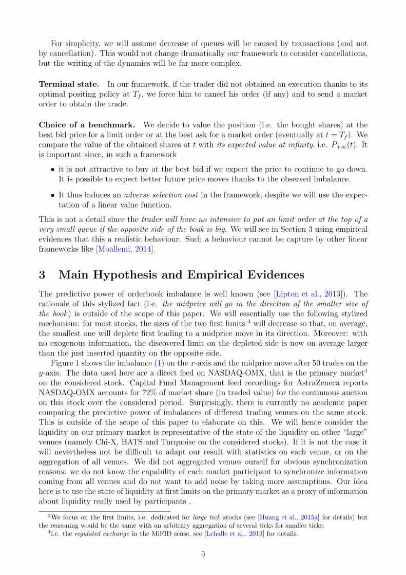
For simplicity, we will assume decrease of queues will be caused by transactions (and notby cancellation). This would not change dramatically our framework to consider cancellations,but the writing of the dynamics will be far more complex.
Terminal state. In our framework, if the trader did not obtained an execution thanks to itsoptimal positing policy at Tf , we force him to cancel his order (if any) and to send a marketorder to obtain the trade.
Choice of a benchmark. We decide to value the position (i.e. the bought shares) at thebest bid price for a limit order or at the best ask for a market order (eventually at t = Tf ). Wecompare the value of the obtained shares at t with its expected value at infinity, i.e. P+∞(t). Itis important since, in such a framework
• it is not attractive to buy at the best bid if we expect the price to continue to go down.It is possible to expect better future price moves thanks to the observed imbalance.
• It thus induces an adverse selection cost in the framework, despite we will use the expec-tation of a linear value function.
This is not a detail since the trader will have no intensive to put an limit order at the top of avery small queue if the opposite side of the book is big. We will see in Section 3 using empiricalevidences that this a realistic behaviour. Such a behaviour cannot be capture by other linearframeworks like [Moallemi, 2014].
3 Main Hypothesis and Empirical Evidences
The predictive power of orderbook imbalance is well known (see [Lipton et al., 2013]). Therationale of this stylized fact (i.e. the midprice will go in the direction of the smaller size ofthe book) is outside of the scope of this paper. We will essentially use the following stylizedmechanism: for most stocks, the sizes of the two first limits 3 will decrease so that, on average,the smallest one will deplete first leading to a midprice move in its direction. Moreover: withno exogenous information, the discovered limit on the depleted side is now on average largerthan the just inserted quantity on the opposite side.
Figure 1 shows the imbalance (1) on the x-axis and the midprice move after 50 trades on they-axis. The data used here are a direct feed on NASDAQ-OMX, that is the primary market4
on the considered stock. Capital Fund Management feed recordings for AstraZeneca reportsNASDAQ-OMX accounts for 72% of market share (in traded value) for the continuous auctionon this stock over the considered period. Surprisingly, there is currently no academic papercomparing the predictive power of imbalances of different trading venues on the same stock.This is outside of the scope of this paper to elaborate on this. We will hence consider theliquidity on our primary market is representative of the state of the liquidity on other “large”venues (namely Chi-X, BATS and Turquoise on the considered stocks). If it is not the case itwill nevertheless not be difficult to adapt our result with statistics on each venue, or on theaggregation of all venues. We did not aggregated venues ourself for obvious synchronizationreasons: we do not know the capability of each market participant to synchronize informationcoming from all venues and do not want to add noise by taking more assumptions. Our ideahere is to use the state of liquidity at first limits on the primary market as a proxy of informationabout liquidity really used by participants .
3We focus on the first limits, i.e. dedicated for large tick stocks (see [Huang et al., 2015a] for details) butthe reasoning would be the same with an arbitrary aggregation of several ticks for smaller ticks.
4i.e. the regulated exchange in the MiFID sense, see [Lehalle et al., 2013] for details.
5

(a) (b)
−0.8 −0.6 −0.4 −0.2 0.0 0.2 0.4 0.6 0.8Imbalance
−8
−6
−4
−2
0
2
4
6
8
Ave
rage
pri
cem
ove
−0.8 −0.6 −0.4 −0.2 0.0 0.2 0.4 0.6 0.8Imbalance
0.35
0.40
0.45
0.50
0.55
0.60
0.65
0.70
0.75
Pct
ofev
ents
Figure 1: (a) The predictive power of imbalance on stock Astra Zeneca: imbalance (just beforea trade) on the x-axis and the expected price move (during the next 50 trades) on the y-axis.(b) distribution of the imbalance just before a trade. From the 2013-01-02 to the 2013-09-30(accounts for 376,672 trades).
Venue AstraZeneca VodafoneBATS Europe 7.16% 7.63%Chi-X 19.27% 20.02%Primary market 72.24% 61.09%Turquoise 1.33% 11.26%
Table 1: Fragmentation of AstraZeneca (compared to Vodafone) from the 2013-01-02 to the2013-09-30
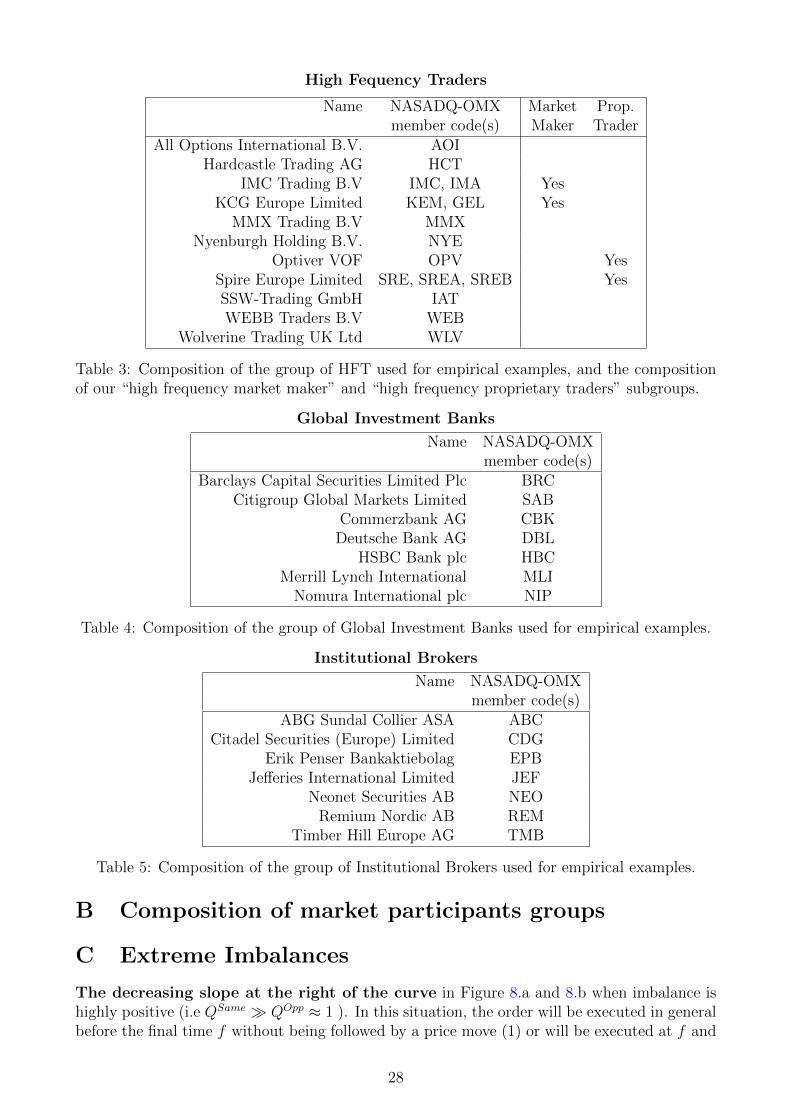
We focus on NASDAQ-OMX because this European market has an interesting property:market members’ identity is known. It implies transactions are labeled by the buyer’s andseller’s names. Almost all trading on NASDAQ Nordic stocks was labelled this way until end of2014 (more details are available in [van Kervel and Menkveld, 2014], because this whole paperis based on this labelling). Note members’ identity is not investors’ names; it is the identifyof brokers or market participants large enough to apply for a membership. High FrequencyParticipants (HFP) are of this kind. Of course some participants (like large asset managementinstitutions) use multiple brokers, or a combination of brokers and their own membership.Nevertheless, one can expect to observe different behaviours when members are different enough.We will here focus on three classes of participants: High Frequency Participants (HFP), globalinvestment banks, and regional investment banks.
The main hypothesis of this paper is some market participants take the state of the order-book into account to accept or not a transaction. We have in mind one participant can investto have a good overview of the microscopic state of the liquidity before inserting or cancellinglimit orders, or before sending a marketable order. On the principle, academic papers haveshown the predictive power of bid-ask imbalance, we try to understand if it is used by somemarket participants, and how to use it.
We will show how optimal control can provide an efficient way to take such information intoaccount. Moreover, latency is of paramount importance when one want to take into account themicroscopic state of liquidity: one can be perfectly aware of liquidity imbalance and know howto use it optimally, but can be prevented to do so because of his latency to matching enginesof exchanges. The lower frequency of a participant, the less number of times he will be able totake value-adding decisions between t = 0 and t = TF .
6

Main hypothesis of this paper: exploitation of imbalance for limit orders. We expectsome market participants to invest in access to data and technology to be able to take profit ofthe informational content of orderbook imbalance. A very simple way to test this hypothesis isto look at orderbook imbalance just before a transaction with a limit order of a given class ofparticipant. We will focus on three classes of agents (i.e. market participants): High FrequencyParticipants (HFP), Global Investment Banks or Brokers, and Regional Investment Banks orBrokers. Table 2 provides descriptive statistics on our these classes of participants in theconsidered database.
Order type Participant type Order side Avg. Imbalance Nbe of events
Limit Global Banks Sell -0.35 62,111Buy -0.38 63,566
HFP Sell -0.32 52,315Buy -0.33 46,875
Instit. Brokers Sell -0.57 6,226Buy -0.52 4,646
Table 2: Descriptive statistics for our three classes of agent. AstraZeneca (2013-01 to 2013-09).
We focus on limit orders since information processing, strategy and latency play a moreimportant role for such orders than for market orders (market orders can be sent blindly, justto finish a small metaorder or to cope with metaorders late on schedule, see [Lehalle et al., 2013]for ellaborations on brokers’ trading strategies).
For the following charts, we use labelled transactions from NASDAQ-OMX5 and thanks totimestamps (and matching of prices and quantities) we synchronize them with orderbook data(recorded from direct feeds by Capital Fund Management). It enables us to snapshot the sizesat first limits on NASDAQ-OMX just before the transaction.
Say for a given participant (i.e. agent) a the quantity at the best bid (respectively best ask)is QBid
τ (a) (resp. QAskτ (a)) just before a transaction at time τ involving a limit order owned
by a. We note Qsameτ (a) := QBid
τ (a) (respectively Qoppositeτ (a) := QAsk
τ (a)) if it was a buy limitorder, or Qsame
τ (a) := QAskτ (a) (respectively Qopposite
τ (a) := QBidτ (a)) if it was a sell limit order.
We normalize the quantities by the best opposite to obtain ρτ (a) = Qsameτ (a)/Qopposite
τ (a)the fraction of the quantity of the same side of the limit order over the quantity on the oppositeside. It is then easy to average over the transactions indexed by timestamps τ to obtain anestimate of this expected ratio for one class of agent:
R(a) =1
Card(T )
∑τ∈T
ρτ (a), limCard(T )→+∞
R(a) = Eτ(
Qsameτ (a)
Qoppositeτ (a)
). (4)
It is even possible to control a potential biais by using the same number of buy and sellexecuted limit orders to compute this “neutralized” average:
Rn(a) =1
Card(T (buy))
∑τ∈T (buy)
ρτ (a) +1
Card(T (sell))
∑τ∈T (sell)
ρτ (a). (5)
Figure 2.a shows the average state of the imbalance (via some estimates of Rn(a), on As-traZeneca from January 2013 to August 2013) for each class of agent (see Tables 3, 4, 5 forlists of NASDAQ-OMX memberships used to identify agents classes). One can see the state ofthe imbalance is different for each class given it “accepted” to transact via a limit order:
5For each transaction, we have a buyer ID, seller ID, a size, a price and a timestamp.
7

(a) (b)
Instit. Brokers Global Banks HFT−0.6
−0.5
−0.4
−0.3
−0.2
−0.1
0.0
0.1
Ave
rage
Imb
alan
ce
Instit. Brokers Global Banks HF MM HF Prop.−0.6
−0.5
−0.4
−0.3
−0.2
−0.1
0.0
0.1
Ave
rage
Imb
alan
ce
Figure 2: Comparison of neutralized orderbook Imbalance Rn(a) at the time of a trade via alimit order (a) for institutional brokers, global investment banks and High Frequency Partic-ipants. (b) Shows a split of HFP between market makers and proprietary traders. It is cleareach type of participant has a different strategy. Data are the ones for AstraZeneca (2013-01to 2013-09).
• Institutional brokers accept a trasaction when the imbalance is largely negative, i.e. theybuy using a limit order while the price is going down. It generates a large adverse selection:they would have wait a little more, the price would have been cheaper. It may be becausethey do not look enough at the orderbook, or they make this choice because they have tobuy fast from risk management reasons on their clients’ orders (in our model with havea waiting cost parameter c that can probably afford to be used to inject such urgency inthe model).
• High Frequency Participants (HFP) accept a transaction when the imbalance is aroundone half of the one when Institutional brokers accept a trade: they make another choice.For sure they look more at the orderbook state before taking a decision. Moreover theycould be more opportunistic: ready to wait the perfect moment instead of being lead byurgency considerations.
If we split HFP between more market making-oriented ones and proprietary trading oneson Figure 2.b we see
– market makers (probably for urgency reasons: they have to alternate buys and sells),accept to trade when the imbalance is more negative than the average of HFP. Theyare probably paid back from this adverse selection by bid-ask spread gains (see[Menkveld, 2013]);
– while proprietary traders are from far the most opportunistic participants of ourpanel, leading them to have a less intense imbalance when they trade via limitorders: they seem to be the ones less suffering from adverse selection.
• Global Investment banks are in between: or their activity is a mix of client executionand proprietary trading (hence we perceive the imbalance when they accept a trade asan average of the two upper ones), or they have specific strategies to accept transactionsvia limit orders, or they invest a little less than HFP in low latency technology, but morethan institutional brokers.
Obviously each class of agent seems to (be able to) exploit differently the state of the orderbookbefore accepting or not a transaction.
8

The value of imbalance for market participants. Now we know classes of agents takedifferently into account the state of orderbook imbalance to accept or not a transaction via alimit order, one can ask what could be the value of such an “high frequency market timing”.
We attempt to measure this value with a combination of NASDAQ-OMX labelled transac-tions and our synchronized market data. That for, we compute the midprice move immediatelybefore and after a class of participant a accepted to transact via a limit order:
∆Pmidδt (τ, a) =
Pmidτ+δt − Pmid
τ
ψ· ετ (a), (6)
where ετ (a) is the “sign” of the transaction (i.e. +1 for a buy and -1 for a sell).A “price profile6” around a trade is the averaging of this price move as a function of δt
(between -5 minutes and +5 minutes); it is an estimate of the “expected price profile” arounda trade:
pa(δt) =1
Card(T )
∑τ∈T
∆Pmidδt (τ, a), lim
Card(T )→+∞pa(δt) = Eτ∆Pmid
δt (τ, a).
(a) (b)
−100 0 100 200 300 400Number of trades
−0.10
−0.08
−0.06
−0.04
−0.02
0.00
0.02
0.04
Ave
rage
mid
-pri
cem
ove
Global Banks
Instit. Brokers
HFT
−100 0 100 200 300 400Number of trades
−0.10
−0.08
−0.06
−0.04
−0.02
0.00
0.02
0.04
Ave
rage
mid
-pri
cem
ove
Global Banks
Instit. Brokers
HF MM
HF Prop.
Figure 3: Midprice move relative to its position when a limit order is executed for (a) an HighFrequency Market Maker, a regional investment bank, and an institutional broker; (b) makesthe difference between HF market makers and HF proprietary traders. AstraZeneca (2013-01to 2013-09).
Figure 3.a and 3.b show the price profiles of our three classes of participants, exhibiting realdifferences beween them. First of all, it confirms the conclusions we draw from Figure 2. Sinceit is always interesting to have a look at dynamical measures of liquidity (see [Lehalle, 2014]for a defense of the use of more dynamical measures of liquidity instead of plain averages):
• It is clear Institutional brokers (green line) are buying while the price is going down.Would they have bought later, they would have obtained a cheaper price. As underlinedearly they probably do it by purpose: they can have urgency reasons or they are using a“trading benchmark” that does pay more attention to peg to the executed volume thanto the execution price (see [Lehalle et al., 2013, Chapter 3] for details about brokers’benchmarks).
• We can see the difference between High Frequency Participants (HFP) and Global in-vestment banks come from the price dynamics before the trade via a limit order : for
6Note this “price profiles” are now used as a standard way to study the behaviour of high frequency tradersin academic papers, see for instance [Brogaard et al., 2012] or [Biais et al., 2016].
9

Investment banks the price was more or less stable, and had to go down so that the limitorder is executed. For HFP the price clearly went up before they bought with a limit order.This implies they inserted their limit order shortly before the trade. In our framework wewill see how cancelling and reinserting limit orders can be a way to implement an optimalstrategy.
• On Figure 3.b we see the difference between HF market makers and HF proprietarytraders: the latter succeed in inserting buy (respectively sell) limit orders and obtainingtransaction while the price is clearly going up (resp. down). After the trade, one canread a difference between them and HF market makers: proprietary traders suffer fromless adverse selection (the cyan curve is a little higher than the red one).
These charts show there is a value in taking liquidity imbalance into account. In the followingsections of this paper we will theoretically show how paying attention to orderbook imbalancecan be valued to insert or cancel limit orders.
The role of latency. Without a fast enough access to the exchange servers, a participantcould “know” the best action to perform (insert or cancel a limit order), but not be able toimplement it before an unexpected transaction. Since low latency has a cost, some participantmay decide to ignore this information and do not access to market feeds, orderbooks states,etc.
In the following sections we will not only provide a theoretical framework to “optimally”exploit oderbook dynamics for limit order placement, but also study its sensitivity to latency,showing how latency can destroy the added value of understanding orderbook dynamics.
In our theoretical framework, we will not study the situations in which the participantknows the best action but cannot implement it on time. We will rather reproduce the case of aparticipant having access to the state of the orderbook at a lower frequency than another. Inpractical cases it will mean this participant will see the state of liquidity with delay.
4 The Dynamic Programming Principle Applied to Limit
Order Placement
4.1 Formalisation of the Model
We will express the control problem for a buy order of a deterministic size q. It can be changedto a sell order with ease. Since our value function is linear in q, this deterministic atomicquantity can be replaced by any random variable independent from other variables with nochange.
Let q be a unit limit order inserted in the first Bid limit of the order book. This order isfollowed by a quantity QAfter and preceded by a quantity QBefore. The first opposite limit hasa quantity QOpp. The quantities QAfter,QBefore and QOpp are multiples of the unit quantity q(see Figure 4 for an illustration).
For simplicity, we neglect the quantity q and set:
QSame = QBefore +QAfter. (7)
It could be changed to QSame = QBefore +QAfter + q ; such a case can be written and studiedsimilarly to what we propose here. The results would nevertheless be different.
10

|Same Opp
QBefore
q
QAfter
QOpp
P (t)Price
Figure 4: Diagram of needed variables for our orderbook model.
Limit order book dynamics. At the beginning, we don’t differentiate between a cancel-lation order and a market order. The order book dynamic can be modeled by four countingprocesses (see Figure 5):
• A counting process NOpp,+t with an intensity λOpp,+(QOpp, QSame) representing the inserted
orders in the opposite limit.
• A counting process NOpp,−t with an intensity λOpp,−(QOpp, QSame) representing the can-
celed orders in the opposite limit.
• A counting process NSame,+t with an intensity λSame,+(QOpp, QSame) representing the in-
serted orders in the Bid limit.
• A counting process NSame,−t with an intensity λSame,−(QOpp, QSame) representing the can-
celed orders in the Bid limit.
These four counting processes depend only on the first limit quantities. Moreover, theBid-Ask symmetry provides us the following relation:{
λOpp,+(QOpp, QSame) = λSame,+(QSame, QOpp)λOpp,−(QOpp, QSame) = λSame,−(QSame, QOpp)
. (8)
|Same Opp
QBefore
q
QAfter
QOpp
P (t)Price
λSame,+
λSame,−
λOpp,+
λOpp,−
Figure 5: Diagram of flows affecting our orderbook model.
11

Hence, the size of the first limits can be written:QOpp(t+ dt) = QOpp(t) + dNOpp,+
t − dNOpp,−t
QBefore(t+ dt) = QBefore(t)− dNSame,−t
QAfter(t+ dt) = QAfter(t) + dNSame,+t − 1QBefore≤0dNSame,−
t
(9)
What happens when QAfter,QBefore or QOpp is totally consumed : First of all, weneglect the probability that at least two of these three events happen simultaneously.
1. When QOpp(t) < 0. The price increases by one tick (keep in mind for a buy order, theopposite is the ask side). Then, we discover a new opposite limit and a new bid quantityis inserted into the bid-ask spread (on the bid side) by other market participants (seeFigure 6). It reads
QOpp(t+ dt) = QDisc(QSamet , QOpp
t )
QBefore(t+ dt) = QIns(QSamet , QOpp
t )QAfter(t+ dt) = 0
(10)
QDisc is the “discovered quantity” and QIns the “inserted quantity”. We model them viacounting processes with respective intensities λDisc(QSame
t , QOppt ) and λIns(QSame
t , QOppt )
that can be function of the orderbook state before the price changing event.
|Same Opp
QBefore
qQAfter
QOpp
P (t) Price
λSame,+
λSame,−
λOpp,+
λOpp,−
Before price move
| |Same Opp
QIns
q
QDisc
P (t) P(t)+1 Price
After price move
Figure 6: Diagram of a upward price change for our model.
2. When QBefore(t) < 0. The optimized limit order is going to be executed. The new stateof the limit order book is the following:
QOpp(t+ dt) = QOpp(t) + dNOpp,+t − dNOpp,−
t
QBefore(t+ dt) = 0
QAfter(t+ dt) = QAfter(t) + dNSame,+t − dNSame,−
t
(11)
3. When QAfter(t) < 0 The price decreases by one tick. then, we discover a new quantity atthe Bid side and market makers insert a new quantity on the opposite side such as:
QOpp(t+ dt) = QIns(QOppt , QSame
t )
QBefore(t+ dt) = QDisc(QOppt , QSame
t )QAfter(t+ dt) = 0
(12)
If the optimized limit order was in the book: it has been executed. Otherwise the pricemoves down and the trader has the opportunity to reinsert a limit order on the top ofQDisc (see Figure 7 for a diagram).
12

|Same Opp
QAfter QOpp
P (t) Price
λSame,+
λSame,−
λOpp,+
λOpp,−
Before price move
| |Same Opp
QDisc
QIns
P(t)-1 P(t) Price
After price move
Figure 7: Diagram of an downward price move in our model.
The control. We consider two types of control C = {s, c}:
• c (like continue): stay in the order book;
• s (like stop): cancel the order and wait for a better orderbook state to reinsert it atthe top of Qsame (Qbid for our buy order). This control will essentially be used to avoidadverse selection, i.e. obtaining a transaction just before a price decrease.
If at the end of T periods the order hasn’t been executed, we cross the spread guaranteeexecution. Once the order is executed, we will compare the execution price to a benchmarkprice (microprice) P∞ that we will describe further.
We set the time step to ∆t and the final time to Tf . Let t0 = 0 < t1 · · · tf−1 < tf = Tfdifferent instants at which the order book is observed, such as tn = n∆t for all n ∈ {0, 1, · · · , f}.We add a terminal time Tf+1 such as Tf+1 = (f + 1)∆t .
Under the following assumption: Between two consecutive instants tn and tn+1 for all n ∈{0, 1, · · · , f − 1}, only five cases can occur:
• 1 unit quantity is added at the Bid side;
• 1 unit quantity is consumed at the Bid side;
• 1 unit quantity is added at the opposite side;
• 1 unit quantity is consumed at the opposite side;
• nothing happens.
We neglect the situation of at least two cases occurring during the same time interval (theprobability of such conjunctions are of the orders of λ2, hence our approximation remains validas far as λ2dt is small compared to one and λ2 is small compared to lambda). Moreover, thetimes arrivals of the orders follow a counting processes which the intensities depend on theimbalance.
Framework 1 (Our setup in few words.). In short, our main assumptions are:
• only one limit order of atomic quantity q is controlled, it is small enough to have noinfluence on orderbook imbalance;
• decrease of queue sizes at first limit is caused by transactions only (no difference betweencancellation and trades);
• queues decrease or increase by one quantity only;
13

• the intensities of point processes (including the ones driving quantities inserted into thebid-ask spread, and driving the quantity discovered when a second limit becomes a firstlimit) are functions of the quantities at best limits only;
• no notable conjunction of multiple events.
We introduce the following Markov chain Un =(Pn, Q
Beforen , QAfter
n , QOppn ,Execn
)where:
• Pn is the mid-price at time tn that takes value in R+.
• QBeforen is the QBefore size at time tn that takes value in N.
• QAftern is the QAfter size at time tn that takes value in N.
• QOppn is the QOpp size at time tn that takes value in N.
• Execn is an additional variable that takes value in {−1, 0, 1}. Execn equals to 1 whenthe order is executed at time tn, 0 when the order is not executed at time tn and -1(a “cemetery state”) when the order has been already executed before. Initially, we fixExec0 = 0.
In the same way, we define NSame,+n , NSame,−
n , NOpp,+n and NOpp,−
n as the values of the countingprocesses NSame,+
t , NSame,−t , NOpp,+
t et NOpp,−t at time tn. The transition probabilities of the
markov chain Un are detailed in Appendix A.
The terminal constraint. The microprice P∞,k is defined such as:
P∞,k = F (QOppk , QSame
k , Pk) = Pk +α
2· Q
Samek −QOpp
k
QOppk +QSame
k
∀k ∈ {0, 1, · · · , f}.
Where α is a predictability parameter that represents the sensitivity to the imbalance.The execution price PExec,k is defined ∀k ∈ {0, 1, · · · , f} such as :
PExec,k =
{Pk + 1
2when Execk = 0
Pk − 12
when Execk ∈ {−1, 1} (when a market order is set).
Let k0 be the execution time: k0 = inf (k ≥ 0,Execk = 1)∧ f . Then, the terminal valuationcan be written:
Zk0 = P∞,(k0+1) − PExec,(k0)
Let U the set of all progressively measurable processes µ := {µk, k < f} valued in {s, c}This problem can be written as a stochastic control problem :
VU0,f = supµ∈U
EU0,µ
(f−1∑i=1
gi(Ui, µi) + gf (Uf )
)
Where gi(Ui, µi) = Zi when Execi = 1 and µi = c and 0 otherwise for all i ∈ {1, · · · , f − 1},and gf (Uf ) = Zf when Execf ∈ {0, 1} and 0 otherwise.
In other words we want to maximize VU0,f = supµ∈U
EU0,µ
(Zk0) which can be reached by the
dynamic programming algorithm:{Gf = ZfGn = max (P c
nGn+1, PsnGn+1) ∀n ∈ {0, 1, · · · , f − 1} (13)
Where Pn represents the transition matrix of the markov chain Un.
14

5 A Qualitative Understanding
The equation (13) provides an explicit forward-backward algorithm that can be solved numer-ically. The following part present the simulation results. For more details about the forward-backward algorithm see Appendix A. This section comments simulation results.
We are going to compare two situations:
• The first one called (NC) corresponds to the case when no control is adopted (i.e wealways stay in the Orderbook).
• The second one called (OC) corresponds to the optimal control case when both controls”c” and ”s” are considered.
Moreover, our simulation results are given for two different cases :
• Framework (CONST): The intensities of insertion and cancellation are constant: λSame,+k =λOpp,+k = 0.06 and λSame,−k = λOpp,−k = 0.1 ∀k ∈ {0, 1, · · · , f}. Under (CONST), the in-serted quantities QIns and discovered quantities QDisc are constant too.
• Framework (IMB): The intensities of cancellation and insertion are functions of theimbalance such as ∀k ∈ {0, 1, · · · , f} :
λOpp,+k
(QOppk , QSame
k
)= λSame,−k
(QOppk , QSame
k
)=
QOppk
β·(QOppk +QSame
k )
λOpp,−k
(QOppk , QSame
k
)= λSame,+k
(QOppk , QSame
k
)=
QSamek
β·(QOppk +QSame
k )
Where β is a predictability parameter that represents the sensitivity to the imbalance.
Moreover, under (IMB), inserted and discovered quantities are computed the following way:
• When QOppk is totally consumed , we setQDisc
k = bθdisc·QOppk c andQIns = bθins·QSame
k c.Where θdisc and θins are coefficients associated to liquidity and b.c is the upper round-ing (this kind of relations is compatible with empirical findings of [Huang et al., 2015b]and different from [Cont and De Larrard, 2013] in which Qdisc = Qins is independant ofliquidity imbalance).
• Similarly when QSame is totally consumed , we set QDisc = bθdisc ·QSamec and QIns =bθins ·QOppc.
5.1 Numerically Solving the Control Problem
5.1.1 Anticipation of Adverse Selection
The cancellation is used by the optimal strategy to avoid adversion selection. For instance,when the quantity on the Same side is extremely lower than the one in the Opposite side, it isexpected to cancel the order to wait for a better future opportunity. The optimal control takesin consideration this effect and cancels the order when such a high adverse selection effect ispresent.
We keep the same notations of Section 4. Let µ := {µk, k < f} a control, we defineEU0,µ (∆P|Exec) = EU0,µ
(P∞,(k0+1) − PExec,(k0)
). EU0,µ (∆P|Exec) depends on the control µ,
the initial state of the limit Orderbook U0 and the terminal time f . The dynamics of the
15

quantity EU0,µ (∆P|Exec) can be written :
EU0,µ
(∆P|Exec
)=
f−1∑i=1
∑states Ui
under µ
1Execi=1 ·(P∞,(i+1) − Pi
)· pUi
+∑
states Uf
under µ
1Execf∈{0,1} ·(P∞,(f+1) − Pf
)· pUf
Where pUi∀i ∈ {0, 1, · · · , f} represents the probability to reach the states Ui starting from
the initial point U0 under µ.The quantity pUican easily be computed knowing the transition
matrix of the markov chain Un (cf. Appendix A). Thusly, thanks to the former equation, thequantity EU0,µ (∆P|Exec) can be directly computed by a forward algorithm that visits all thepossible states of the markov chain Un under the control µ.
The quantity EU0,µ (∆P|Exec) is interesting because it corresponds exactly to the quantityto be maximize by our optimal control problem and represents as well the profitability/tradeof an agent.
Let µc the control associated to the case where we always choose to stay in the limitOrderbook (i.e NC). The Figure 8.a represents the variation of EU0,µ∗ (∆P|Exec) (i.e OC) andEU0,µc (∆P|Exec) (i.e NC) when the initial imbalance of the Orderbook moves under (CONST). In Figure 8.a, Blue points refer to the cases where it is better to stay in the Orderbookat the beginning while red points refer to the cases where it is better to cancel the order atthe beginning. The intial parameters are fixed such as λSame,+ = λOpp,+ = 0.06, λSame,− =λOpp,− = 0.1, α = 24, QDisc = 4, QIns = 2, f = 4 and P0 = 10. Moreover, the different valuesof the initial imbalance are obtained by varying QOpp
0 from 2 to 10 and QAfter0 from 2 to 10
while QBefore0 is kept constant equal to 0. We recall that the order is executed when QAfter is
consumed (cf. appendix A for more details).In Figure 8.b, we represent the same thing as in Figure 8.a but under the framework (IMB).
In Figure 8.b, The intial parameters are fixed such as β = 3, θdisc = 3, θins = 0.6, α = 24, f = 4and P0 = 10. Similarly, the different values of the initial imbalance are obtained by varyingQOpp
0 from 2 to 10 and QAfter0 from 2 to 10 while QBefore
0 is kept constant equal to 0.
(a) (b)
−0.8 −0.6 −0.4 −0.2 0.0 0.2 0.4 0.6 0.8Initial imbalance
−8
−6
−4
−2
0
2
4
6
8
EU
0,µ
(∆P|E
xec)
NC
OC
First action is stay
First action is cancel
−0.8 −0.6 −0.4 −0.2 0.0 0.2 0.4 0.6 0.8Initial imbalance
−8
−6
−4
−2
0
2
4
6
EU
0,µ
(∆P|E
xec)
NC
OC
First action is stay First action is cancel
Figure 8: EU0,µ∗ (∆P|Exec) move relative to initial imbalance when intensities are constant(CONST) in (a) and when they are variable (IMB) with β = 3 in (b).
In Figure 8, the expected price move given an execution has been obtain according toframeworks (CONST) (Figure 8.a) and (IMB) (Figure 8.b), comparing the simulated optimal
16

strategy (OC) to the simple “join the bid” (NC) one.
The main effect to note on these curves is the way the optimal control anticipate adversionselection. When Imbalance is highly negative, we cancel first the order (red points) to takeadvantage from a better futur opportunity. However, as our order has a unit size, the algorithmwait until the last moment to cancel the order. That’s why, we took α = 24 to accentuate theimbalance effect. We notice that the (OC) case provides better result than the (NC) case (cf.Figure 10). This point is going to be detailed further.
Appendix C explains the downward slopes at the left of Figures 8.a and 8.b.
5.1.2 Influence of Non Constant Intensities
The framework (CONST) is a simplified version of the problem introduced first to shed lighton some stylized facts like the adverse selection risk. The framework (IMB) is a more realisticand dynamic version of the problem because inserted and cancelled intensities depend on thecurrent state of the markov chain Un. Moreover, the inserted and discovered quantities QIns
and QDisc depend as well on the current state of the markov chain Un. In this part, we wantto compare these two models.
The Figure 9.a represents the variation of EU0,µ∗ (∆P|Exec) when the initial imbalance ofthe limit order book moves, under (CONST) and (IMB). In Figure 9.a, Blue points refer tothe cases where it is better to stay in the Orderbook at the beginning while red points referto the cases where it is better to cancel the order at the beginning. We keep the same intialparameters of the Figure 8.
Let µ a control, we define pLU0,µthe probability that the price Pn moves to the left starting
from the intial state U0 and under the control µ. The quantity pLU0,µcan be written :
pLU0,µ=
f∑i=0
∑states Ui
under µ
EU0,µ
(1{Pi+1=Pi−1}
)
Similarly, we define pRU0,µthe probability that the price Pn moves to the right starting from the
intial state U0 and under the control µ such as :
pRU0,µ=
f∑i=0
∑states Ui
under µ
EU0,µ
(1{Pi+1=Pi+1}
)
Thanks to the above equations, the quantities pRU0,µand pLU0,µ
can be directly computed by aforward algorithm that visits all the possible states of the markov chain Un.
In Figure 9.b, we represent the variation of pLU0,µunder (CONST) (i.e points in blue) and
(IMB) (i.e points in green) when the initial imbalance moves. The circle sizes are proportionalto the number of times the price moves downward (i.e. in an adversely selection direction).When the price moves downward frequently, the point size is huge. We represent as well thevariation of pRU0,µ
under (CONST) (i.e points in red) and (IMB) (i.e yellow points) when theinitial imbalance moves. Again, the circle sizes are proportional to the number of times theprice moves upward (i.e. worst price). We keep the same intial parameters of the Figure 8.
Figure 9 shows the imbalance effect.When intensities depend on imbalance (IMB) itchanges the transition probabilities by giving more weights to some events and less to others.For instance, assume imbalance is highly positive (cf. Figure 14). In the first case (cf. orderexecuted before f) ∆P ≈ 1 while in the second case (cf. order executed at f) ∆P ≤ 1
2(it
17

(a) (b)
−0.8 −0.6 −0.4 −0.2 0.0 0.2 0.4 0.6 0.8Initial imbalance
−8
−6
−4
−2
0
2
4
6
8EU
0,µ
(∆P|E
xec)
variable intensities (IMB)
constant intensities (CONST)
initial control c
initial control s
−0.8 −0.6 −0.4 −0.2 0.0 0.2 0.4 0.6 0.8 1.0Initial imbalance
0.00
0.02
0.04
0.06
0.08
0.10
0.12
0.14
pL U0,µ-pUR
0,µ
Proba price change left, constant intensities (CONST)
Proba price change right, constant intensities (CONST) Proba price change left, variable intensities (IMB)
Proba price change right, variable intensities (CONST)
Figure 9: (a) EU0,µ∗ (∆P|Exec) move relative to initial imbalance under (CONST) and (IMB).(b) pLU0,µ
and pRU0,µmove relative to initial imbalance under (CONST) and (IMB).
depends on how QDisc and QIns are computed but it remains a sensible value of ∆P ). AsFigure 9.b shows that more weight is given to the second case when intensities depend on theimbalance (IMB). Consequently, it is expected to find EU0,µ∗ (∆P|Exec) lower when intensitiesare variable (IMB). The same reasoning explains the shape of EU0,µ∗ (∆P|Exec) when imbalanceis highly negative.
5.1.3 Price Improvement
Being active is better than being inactive. The results obtained in the optimal control(OC) case are better than the ones without it (NC). In fact, by cancelling and taking intoaccount liquidity imbalance, we can be more efficient than just staying in the orderbook.
The Figure 10.a represents the variation of the price improvement due to the control:EU0,µ∗ (∆P|Exec)−EU0,µc (∆P|Exec) when the initial imbalance of the orderbook moves, under(CONST) and (IMB).
Similarly, The Figure 10.b represents the variation of EU0,µ∗ (P|Exec)−EU0,µc (P|Exec) whenthe initial imbalance of the limit Orderbook moves, under (CONST) and (IMB).
(a) (b)
−0.8 −0.6 −0.4 −0.2 0.0 0.2 0.4 0.6 0.8Initial Imbalance
−0.2
0.0
0.2
0.4
0.6
0.8
1.0
1.2
1.4
1.6
EU
0,µ∗(
∆P|E
xec
)-EU
0,µClass(∆
P|E
xec
)
constant intensities (CONST)
variable intensities (IMB)
−0.8 −0.6 −0.4 −0.2 0.0 0.2 0.4 0.6 0.8Initial Imbalance
−0.8
−0.7
−0.6
−0.5
−0.4
−0.3
−0.2
−0.1
0.0
0.1
EU
0,µ∗(
P|E
xec
)-EU
0,µClass(
P|E
xec
)
constant intensities (CONST)
variable intensities (IMB)
Figure 10: (a) EU0,µ∗ (∆P|Exec) − EU0,µc (∆P|Exec) move relative to initial imbalance under(CONST) and (IMB). (b) EU0,µ∗ (P|Exec) − EU0,µc (P|Exec) move relative to initial imbalancemove relative to initial imbalance under (CONST) and (IMB).
Figure 10 deserves the following comments:
18

• As expected, the optimal control provides better results than a blind “follow the bid”strategy. In Figure 10.a we can see the price improvement is non-negative because ouralgorithm maximize E (∆P). When the imbalance is highly positive, the error is close to0 while when imbalance is highly negative the error becomes higher than 0 by avoidingadverse selection. Similarly, in Figure 10.b we can see that the optimal strategy allowsus to buy our order with a lower average price when imbalance is highly negative by pre-venting from adverse selection. Moreover, this effect can be accentuated when intensitiesdepend on the imbalance.
• Indirectly, maximizing EU0,µ (∆P|Exec) leads to the minimization of the price.
5.1.4 Average Duration of Optimal Strategies
Thanks to the optimal control strategy we can get better results by choosing to be executed inthe best market condition. Figure 11.a represents the average strategy duration when the initialimbalance moves in (NC) and (OC) case under the framework (CONST). The intial parametersare fixed such as λSame,+ = λOpp,+ = 0.06, λSame,− = λOpp,− = 0.1, α = 10, QDisc = 4, QIns = 2,f = 4 and P0 = 10. Figure 11.b represents the same thing as Figure 11.a but under framework(IMB). In this case, the intial parameters are fixed such as β = 4, θdisc = 3, θins = 0.6, α = 10,f = 4 and P0 = 10 Finally, Figure 11.c represents the stay ratio in (NC) and (OC) caseunder (IMB) when the initial imbalance moves. Figure 11 is computed with the same initialparameters as Figure 11.b. In Figure 11.a, 11.b and 11.c, the different values of the initialimbalance are obtained by varying QOpp
0 from 2 to 10 and QAfter0 from 2 to 10 while QBefore
0 iskept constant equal to 0.
Figure 11 shows
• In both Figure 11.a and 11.b, the average strategy duration of the optimal control isalways higher than the non-optimal one. It is an expected result because under theoptimal control we can cancel our order and then choose to postpone our execution.Moreover, we can see that the algorithm choose to cancel the order when high adverseselection is present (i.e the imbalance is highly negative). Consequently, the averagestrategy duration of the optimal control is strictly greater than the non-optimal onewhen the imbalance is highly negative.
• In Figure 11.b, when intensities depend on the imbalance (IMB), we can see a decreasingtrend of the average strategy duration. In fact, under (IMB), when imbalance is highlypositive, more weights are given to events that delay execution. For instance, whenimbalance is highly positive, the Bid queue is a way larger than the Opposite one, thenthe probability to consume an order in the Bid side is low, that’s why it is expected towait more. The same reasoning, shows that when the imbalance is highly negative under(IMB), more weights are given to events that accelerate execution. Moreover, Figure 11.cshows that we become more active when high adverse selection is present. Actually, whenhigh adverse selection (i.e imbalance negative) is present, the stay ratio decreases andconsequently the cancel ratio increases.
5.1.5 Influence of the Terminal Constraint
In this paragraph, we want to shed light on two stylized facts:
• The first one is based on the idea that we can perform better under good initial marketcondition if we have more time left.
19

(a) (b)
−1.0 −0.8 −0.6 −0.4 −0.2 0.0 0.2 0.4 0.6 0.8Initial Imbalance
3.0
3.1
3.2
3.3
3.4
3.5A
vera
gest
rate
gyd
ura
tion
OC
NC
First control is cancel
First control is stay
−1.0 −0.8 −0.6 −0.4 −0.2 0.0 0.2 0.4 0.6 0.8Initial Imbalance
1.8
1.9
2.0
2.1
2.2
2.3
2.4
2.5
Ave
rage
stra
tegy
du
rati
on
OC
NC
First action is cancel
First action is stay
(c)
−1.0 −0.8 −0.6 −0.4 −0.2 0.0 0.2 0.4 0.6 0.8Initial Imbalance
0.65
0.70
0.75
0.80
0.85
0.90
0.95
1.00
1.05
Sta
yra
tio
% stay under NC
% stay under OC
First control is cancel
First control is stay
Figure 11: Average strategy duration as a function of (a) the initial imbalance under (CONST)and (b) initial imbalance under (IMB). (c) Stay ratio as a function of the initial imbalanceunder (IMB).
• The second one is based on the idea that we become highly active when we are close tothe terminal time.
(a) (b)
1 2 3 4 5 6 7Remaining time
−1.6
−1.4
−1.2
−1.0
−0.8
−0.6
−0.4
−0.2
0.0
EU
0,µ
(∆P|E
xec)
Constant intensities
Variable intensities
1 2 3 4 5 6 7Remaining time
0.1
0.2
0.3
0.4
0.5
0.6
0.7
0.8
0.9
Sta
y/C
ance
lra
tio
% cancel time
% stay time
Figure 12: (a) EU0,µ∗ (∆P|Exec) move relative to remaining time under (CONST) and (IMB).(b) stay cancel ratio move relative to remaining time to maturity under (IMB).
In Figure 12.a, we represents the variation of the adverse selection EU0,µ∗ (∆P|Exec) whenthe remaining time moves under (CONST) and (IMB). The initial imbalance is fixed equal to
20

-0.5. Thanks to the Figure 12.a, we can see that more time we have better we can do. However,
the concavity of the curve shows that the marginal performance∂E(∆P)t
∂tis decreasing. Moreover,
Figure 12.a shows also that EU0,µ∗ (∆P|Exec) may converge to a limit value when maturity timetends to infinity. Since the markov chain Un is ergodic (cf. [Huang et al., 2015b]), we believethat this limit value is unique and independent of the initial state of the Orderbook.
In Figure 12.b, we represent the percentage of times where we cancel our order and thepercentage of times where we decide to stay in the Orderbook under the optimal control µ∗
when remaining time to maturity moves under (CONST) and (IMB). The initial imbalance isfixed to -0.5. Thanks to Figure 12.b, we can see that we become more active when we are closeto the maturity time. In fact, when two periods are left to the maturity, we choose to cancelmore times while when six periods are left we prefer to stay in the Orderbook.
5.2 The Price of Latency
Defintion : In Section 4, we have defined the markov chain Un which corresponds to a marketparticipant enabled to change his control at each period. A slower participant will not reactat each limit orderbook move. Hence, he can be modelled by the markov chain Uτn where τcorresponds to a latency factor such as τ ∈ N∗.
Using notations of the previous sections, we define Zτ,f as the final constraint associated tothe Markov chain Uτn. Thus, we define the latency cost of a participant with a latency factorτ such as :
LatencyU0,f (τ) = VU0,f − VU0,f,τ ∀τ ∈ N∗ (14)
Where VU0,f,τ = supµ∈U
EU0,µ (Zτ,f ).
By adapting the same numerical forward-backward algorithm, the latency cost can be com-puted numerically.
In Figure 13.a, we can see the variation of the latency cost when the latency factor τchanges under (CONST) and (IMB). The intial parameters are fixed such as β = 3, θ1 = 3,θ2 = 0.6, α = 2, f = 5 and P0 = 10. The initial imbalance is fixed to 0.5 with an initial stateQAfter
0 = 2,QBefore0 = 0 and QOpp
0 = 6.The Figure 13.b represents the variation of the latency cost for different value of the pre-
dictability parameter α when intensities depend on the imbalance.
(a) (b)
1.5 2.0 2.5 3.0 3.5 4.0 4.5 5.0 5.5Latency
−50
0
50
100
150
200
250
Lat
ency
cost
(F1)
(F2)
1.5 2.0 2.5 3.0 3.5 4.0 4.5 5.0 5.5Latency
−500
0
500
1000
1500
2000
2500
3000
Lat
ency
cost
α=2
α=5
α=10
Figure 13: (a) Latency cost move relative to latency factor τ under (CONST) and (IMB). (b)Latency cost move relative to latency factor τ under (IMB) for different values of α.
The numerical results shows :
21

• The latency cost increases exponentially with the latency factor τ (cf. Figure 13.a).Thusly, more slow we are more cost we will pay. The latency cost is amplified whenintensities are variable (cf. Figure 13.a).
• The latency cost is higher when we are more sensitive to adverse selection (i.e α is big)(cf. Figure 13.b).
Consequently, the added value of exploiting a knowledge on liquidity imbalance is erodedby latency: being able to predict future liquidity consuming flows is of less use if you can’tcancel and reinsert your limit orders at each change in the orderbook state. For instance, whentwo agents act optimally according the same criteria, the faster will gain more profit than theslower. Moreover, agents who overreact to each imbalance move will have higher latency costthan patient agents.
6 Conclusion
We have used NASDAQ-OMX labelled data to show market participants accept or refusetransactions via limit orders as a function of liquidity imbalance. It is not an exhaustive studyon this exchange from the north of Europe (we focus on AstraZeneca from January 2013 toSeptember 2013). We first show orderbook imbalance has a predictive power on future mid pricemove. We then focussed on three types of market participants: Institutional brokers, GlobalInvestment Banks (GIB) and High Frequency Participants (HFP). Data show the former acceptto trade when the imbalance is more negative (i.e. they buy or sell when the pressure is upwardor downwards) than GIB, themselves accepting a less negative imbalance than HFP. Moreover,when we split HFP between high frequency market makers and high frequency proprietarytraders, we see HFPT achieve to buy via limit orders when the imbalance is very small. Wecomplete this analysis with the dynamics of prices around limit orders execution, showing howparticipant use strategically their limit orders.
Then we propose a theoretical framework to control limit orders when liquidity imbalancecan be used to predict future price move. Our framework includes potential adverse selection.We use the dynamic programming principle to provide a way to solve it numerically and exhibitsimulations. We show the solutions of our framework have commonalities with our empiricalfindings.
In a last Section we show how the capability of exploiting imbalance predictability usingoptimal control decreases with latency: the trader has less time to put in place sophisticatedstrategies, hence he cannot take profit of any strategy gain.
The difficult point of using limit orders is adverse selection: when you buy, it is easy toobtain a transaction when the price is going down, but it is not a good way to obtain a tradesince few seconds later, the price will be better. Nevertheless it is not enough to cancel youorder if you know the price will go down (you can rely on liquidity imbalance to have someviews on the future price direction), because when you will reinsert it will be on the top of thebid queue, and you will probably never obtain a transaction: the price will go up again beforeyour limit order has been executed.
Our framework includes all these effects, hence it makes the choice between waiting in thequeue or leaving it when the probability the price will go down is too high. Of course theposition of the limit order in the queue is taken into account by our controller.
22

This leads to a quantitative way to understand market making and latency: if a marketmaker is fast enough, he will be able to play this insert and cancel and re-insert game to reactto his observation of liquidity imbalance. In our framework we use the difference betweenthe sizes of the first bid and ask queues as a proxy of liquidity imbalance, in the real wordmarket participants can use a lot of other information (like liquidity imbalance on correlatedinstruments, or realtime news feeds).
In such a context speed can be seen as a protection to adverse selection, potentially reducingthe cost to make the market. Within this viewpoint, high frequency actions do not add noiseto the price formation process (as opposite to the viewpoint of [Budish et al., 2015]) but allowsmarket makers to offer better quotes. At this stage, we do not conclude speed is good forliquidity because:
• we only focussed on one limit order, we should go towards a framework similar to the oneof [Gueant et al., 2013] to conclude on the added value of imbalance for the whole marketmaking process, but it will be too sophisticated at this stage.
• it is not fair to draw conclusions from a knowledge of the theoretical optimal behaviourof one market participant; to go further we should model the game played by all partic-ipants, similarly to what have been done in [Lachapelle et al., 2016]. Again it is a verysophisticated work.
• Last but not least, any conclusion on the added value of low latency and high frequencymarket making should take into account market conditions. Its value could change withthe level of stress of the price formation.
On overall, this work shows imbalance is used by participants, and provides a theoreticalframework to play with limit order placement. It can be used by practitioners. More impor-tantly, we hope other researchers will extend our work in different directions to answer to morequestions, and we will ourself continue to work further to understand better liquidity formationat the smallest time scales.
Acknowledgements. Authors would like to thank Sasha Stoıkov and Jean-Philippe Bouchaudfor discussions about orderbook dynamics and optimal placement of limit orders that motivatedthis paper. Moroever, authors would like to underline the work of Gary Sounigo (during hisMasters Thesis) and Felix Patzelt (during a post-doctoral research), who worked hard at Capi-tal Fund Management (CFM) to understand how to align NASDAQ-OMX labeled transactionsto direct datafeed of orderbook dynamics.
References
[Almgren and Lorenz, 2006] Almgren, R. and Lorenz, J. (2006). Bayesian adaptive tradingwith a daily cycle. Journal of Trading.
[Bacry et al., 2014] Bacry, E., Iuga, A., Lasnier, M., and Lehalle, C.-A. (2014). Market Impactsand the Life Cycle of Investors Orders. Social Science Research Network Working PaperSeries.
[Besson et al., 2016] Besson, P., Pelin, S., and Lasnier, M. (2016). To cross or not to cross thespread: that is the question! Technical report, Kepler Cheuvreux, Paris.
[Biais et al., 2016] Biais, B., Declerck, F., and Moinas, S. (2016). Who supplies liquidity, howand when? Technical report, BIS Working Paper.
23

[Bouchaud et al., 2004] Bouchaud, J.-P., Gefen, Y., Potters, M., and Wyart, M. (2004). Fluc-tuations and response in financial markets: the subtle nature of ’random’ price changes.Quantitative Finance, 4(2):176–190.
[Brogaard et al., 2012] Brogaard, J., Baron, M., and Kirilenko, A. (2012). The Trading Profitsof High Frequency Traders. In Market Microstructure: Confronting Many Viewpoints.
[Budish et al., 2015] Budish, E., Cramton, P., and Shim, J. (2015). The High-Frequency Trad-ing Arms Race: Frequent Batch Auctions as a Market Design Response. Quarterly Journalof Economics, 130(4):1547–1621.
[Cont, 2001] Cont, R. (2001). Empirical properties of asset returns: stylized facts and statisticalissues. Quantitative Finance, 1(2):223–236.
[Cont and De Larrard, 2013] Cont, R. and De Larrard, A. (2013). Price Dynamics in a Marko-vian Limit Order Book Market. SIAM Journal for Financial Mathematics, 4(1):1–25.
[Dayri and Rosenbaum, 2015] Dayri, K. and Rosenbaum, M. (2015). Large Tick Assets: Im-plicit Spread and Optimal Tick Size. Market Microstructure and Liquidity, 01(01):1550003.
[Fodra and Pham, 2013] Fodra, P. and Pham, H. (2013). Semi Markov model for market mi-crostructure.
[Fricke and Gerig, 2014] Fricke, D. and Gerig, A. (2014). Too Fast or Too Slow? Determiningthe Optimal Speed of Financial Markets. Technical report, SEC.
[Gueant et al., 2012] Gueant, O., Lehalle, C.-A., and Fernandez-Tapia, J. (2012). Opti-mal Portfolio Liquidation with Limit Orders. SIAM Journal on Financial Mathematics,13(1):740–764.
[Gueant et al., 2013] Gueant, O., Lehalle, C.-A., and Fernandez-Tapia, J. (2013). Dealing withthe inventory risk: a solution to the market making problem. Mathematics and FinancialEconomics, 4(7):477–507.
[Harris, 2013] Harris, L. (2013). Maker-taker pricing effects on market quotations. Unpublishedworking paper. University of Southern California, San Diego, CA.
[Huang et al., 2015a] Huang, W., Lehalle, C.-A., and Rosenbaum, M. (2015a). How to predictthe consequences of a tick value change? Evidence from the Tokyo Stock Exchange pilotprogram.
[Huang et al., 2015b] Huang, W., Lehalle, C.-A., and Rosenbaum, M. (2015b). Simulating andanalyzing order book data: The queue-reactive model. Journal of the American StatisticalAssociation, 10(509).
[Jaisson, 2014] Jaisson, T. (2014). Market impact as anticipation of the order flow imbalance.
[Kyle, 1985] Kyle, A. P. (1985). Continuous Auctions and Insider Trading. Econometrica,53(6):1315–1335.
[Lachapelle et al., 2016] Lachapelle, A., Lasry, J.-M., Lehalle, C.-A., and Lions, P.-L. (2016).Efficiency of the Price Formation Process in Presence of High Frequency Participants: aMean Field Game analysis. Mathematics and Financial Economics, 10(3):223–262.
[Lehalle, 2014] Lehalle, C.-A. (2014). Towards dynamic measures of liquidity. AMF ScientificAdvisory Board Review, 1(1):55–62.
24

[Lehalle et al., 2013] Lehalle, C.-A., Laruelle, S., Burgot, R., Pelin, S., and Lasnier, M. (2013).Market Microstructure in Practice. World Scientific publishing.
[Lipton et al., 2013] Lipton, A., Pesavento, U., and Sotiropoulos, M. G. (2013). Trade arrivaldynamics and quote imbalance in a limit order book.
[Lo et al., 2002] Lo, A. W., MacKinlay, C., and Zhan, J. (2002). Econometric models of limit-order executions. Journal of Financial Economics, 65(1):31–71.
[Menkveld, 2013] Menkveld, A. J. (2013). High Frequency Trading and The New-Market Mak-ers. Journal of Financial Markets, 16(4):712–740.
[Moallemi, 2014] Moallemi, C. C. (2014). The Value of Queue Position in a Limit Order Book.In Abergel, F., Bouchaud, J.-P., Foucault, T., Lehalle, C.-A., and Rosenbaum, M., editors,Market Microstructure: Confronting Many Viewpoints. Louis Bachelier Institute.
[Stoıkov, 2014] Stoıkov, S. (2014). Time is Money: Estimating the Cost of Latency in Trading.In Abergel, F., Bouchaud, J.-P., Foucault, T., Lehalle, C.-A., and Rosenbaum, M., edi-tors, Market Microstructure: Confronting Many Viewpoints, Paris. Louis Bachelier Institute.sasha14book.
[Toth et al., 2012] Toth, B., Eisler, Z., Lillo, F., Kockelkoren, J., Bouchaud, J. P., and Farmer,J. D. (2012). How does the market react to your order flow? Quantitative Finance,12(7):1015–1024.
[van Kervel and Menkveld, 2014] van Kervel, V. and Menkveld, A. (2014). Do High-FrequencyTraders Engage in Predatory Trading? Technical report, VU University Amsterdam.
[Zarinelli et al., 2015] Zarinelli, E., Treccani, M., Farmer, J. D., and Lillo, F. (2015). Beyondthe square root: Evidence for logarithmic dependence of market impact on size and partici-pation rate. Market Microstructure and Liquidity, 1(2). lastlillo.
25

A Transition probabilities of the markov chain Un
When the first limits are totally consumed, new quantities QDiscn and QIns
n are inserted in theorder book. We introduce then µn the joint distribution of the random variables QDisc
n et QInsn
at time tn. We consider these two variables independent from their past and independent fromthe counting processes NSame,+, NSame,−, NOpp,− and NOpp,+. However, QDisc
n and QInsn can be
correlated at time tn.Let n ∈ {0, 1, · · · , f}, p ∈ R+, qbef ∈ N, qaft ∈ N, qopp ∈ N, qdisc ∈ N, qins ∈ N and
e ∈ {−1, 0, 1}
• When the order has been executed before tn (i.e e = 1 or e = −1),then :
P(c)(Un+1 = (p, qbef , qaft, qopp,−1)/Un = (p, qbef , qaft, qopp, e)
)= 1 (15)
When the order is executed a dead center is reached and both quantities and the priceremain unchanged.
• When the order isn’t executed at tn (i.e e = 0), and :
A unit quantity is added to QOpp , under control ”c”, the transition probability isthe following :
P(c)(Un+1 = (p, qbef , qaft, (qopp + 1) , e)|Un = (p, qbef , qaft, qopp, e)
)= P(
{NOpp,+n+1 −NOpp,+
n = 1}∩{NOpp,−n+1 −NOpp,−
n = 0}
∩{NSame,+n+1 −NSame,+
n = 0}∩{NSame,−n+1 −NSame,−
n = 0}
)
= λOpp,+n ∆t
(1− λOpp,−n ∆t
) (1− λSame,−n ∆t
) (1− λSame,+n ∆t
).
Under control ”s”, nothing changes except that the order is cancelled and potentiallyinserted at the next step such as QBef
n+1 = qbef + qaft and QAftn+1 = 0.
A unit quantity is cancelled from to QOpp , under control ”c”, we differentiatebetween two cases:
1. When qopp > 1:
P(c)(Un+1 = (p, qbef , qaft, (qopp − 1) , e)|Un = (p, qbef , qaft, qopp, e)
)= P(
{NOpp,+n+1 −NOpp,+
n = 0}∩{NOpp,−n+1 −NOpp,−
n = 1}
∩{NSame,+n+1 −NSame,+
n = 0}∩{NSame,−n+1 −NSame,−
n = 0}
)
= λOpp,−n ∆t
(1− λOpp,+n ∆t
) (1− λSame,−n ∆t
) (1− λSame,+n ∆t
).
Under control ”s”, nothing changes except that QBefn+1 = qbef + qaft and QAft
n+1 = 0.
2. When qopp ≤ 1, the price increase by one tick :
P(c)(Un+1 = (p+ 1, qins, 0, qdisc, e) | Un = (p, qbef , qaft, 1, e)
)= λ−Ask∆t
(1− λ+Ask∆t
) (1− λ−∆t
) (1− λ+∆t
)µn+1(qdisc, qins).
Under control ”s”, the last formula does’nt change.
26

A unit quantity is added to QSame , under control ”c” we have :
P(c)(Un+1 = (p, qbef , qaft + 1, qopp, e)|Un = (p, qbef , qaft, qopp, e)
)= λSame,+n ∆t
(1− λOpp,+n ∆t
) (1− λOpp,−n ∆t
) (1− λSame,−n ∆t
).
Under control ”s”, nothing changes except that QBefn+1 = qbef + qaft + 1 and QAft
n+1 = 0.
A unit quantity is cancelled from QSame , under control ”c”, we distinguish againthree cases :
1. When(qbef > 1 and qaft ≥ 0
)or(qbef = 1 and qaft ≥ 1
):
P(c)(Un+1 = (p, qbef − 1, qaft, qopp, e)|Un = (p, qbef , qaft, qopp, e)
)= λSame,−n ∆t
(1− λOpp,+n ∆t
) (1− λOpp,−n ∆t
) (1− λSame,+n ∆t
).
We suppose that our order is executed when QAftern is consumed. Under control ”s”,
nothing changes except that QBefn+1 = qbef + qaft − 1 and QAft
n+1 = 0.
2. When qbef = 0 and qaft > 1:
P(c)(Un+1 = (p, 0,
(qaft − 1
), qopp, 1)|Un = (p, qbef , qaft, qopp, e)
)= λSame,−n ∆t
(1− λOpp,+n ∆t
) (1− λOpp,−n ∆t
) (1− λSame,+n ∆t
).
Under control ”s”, nothing changes except that QBefn+1 = qbef + qaft − 1, QAft
n+1 = 0and Execn+1 = 0.
3. When qbef + qaft = 1 :
P(c)(Un+1 = (p, qdisc, 0, qins, 1)|Un = (p, 0, qaft, qopp, e)
)= λSame,−∆t
(1− λOpp,+∆t
) (1− λOpp,−∆t
) (1− λSame,+∆t
).
Under control ”s”, nothing changes except that Execn+1 = 0.
Nothing happens in the limit order book with probability(1− λSame,−∆t
) (1− λOpp,+∆t
) (1− λOpp,−∆t
) (1− λSame,+∆t
).
• For all the remaining cases the transition probability is null.
Remark. By taking in consideration the different cases and neglecting the terms withorder strictly superior than 1 in ∆t, we have for any control i ∈ {c, s}:∑
statesUnstatesUn+1
∫(N+)2
P(i)(Un+1|Un) µn+1(d qdisc, d qins)
≈ 1 + λ+Ask∆t + λ−Ask∆t + λ+∆t + λ−∆t.
Consequently, if λ+Ask∆t + λ−Ask∆t + λ+∆t + λ−∆t = o(1) ( which is true when ∆t is small),we end up with for any control i ∈ {c, s}:∑
statesUnstatesUn+1
∫(N+)2
P(i)(Un+1/Un)µn+1(d qdisc, d qins) ≈ 1 (16)
27
High Fequency Traders
Name NASADQ-OMX Market Prop.member code(s) Maker Trader
All Options International B.V. AOIHardcastle Trading AG HCT
IMC Trading B.V IMC, IMA YesKCG Europe Limited KEM, GEL Yes
MMX Trading B.V MMXNyenburgh Holding B.V. NYE
Optiver VOF OPV YesSpire Europe Limited SRE, SREA, SREB YesSSW-Trading GmbH IATWEBB Traders B.V WEB
Wolverine Trading UK Ltd WLV
Table 3: Composition of the group of HFT used for empirical examples, and the compositionof our “high frequency market maker” and “high frequency proprietary traders” subgroups.
Global Investment Banks
Name NASADQ-OMXmember code(s)
Barclays Capital Securities Limited Plc BRCCitigroup Global Markets Limited SAB
Commerzbank AG CBKDeutsche Bank AG DBL
HSBC Bank plc HBCMerrill Lynch International MLI
Nomura International plc NIP
Table 4: Composition of the group of Global Investment Banks used for empirical examples.
Institutional Brokers
Name NASADQ-OMXmember code(s)
ABG Sundal Collier ASA ABCCitadel Securities (Europe) Limited CDG
Erik Penser Bankaktiebolag EPBJefferies International Limited JEF
Neonet Securities AB NEORemium Nordic AB REM
Timber Hill Europe AG TMB
Table 5: Composition of the group of Institutional Brokers used for empirical examples.
B Composition of market participants groups
C Extreme Imbalances
The decreasing slope at the right of the curve in Figure 8.a and 8.b when imbalance ishighly positive (i.e QSame � QOpp ≈ 1 ). In this situation, the order will be executed in generalbefore the final time f without being followed by a price move (1) or will be executed at f and
28

followed by a price move (2). In both cases, the final constraint ∆P is positive (see graph 14).Given that ∆P in case (2) is lower than ∆P in case (1) and situation (2) occurs more frequentlywhen imbalance is highly positive, it is expected to find a decreasing slope at the right of thecurve.
|q
QAfter
QSame
Same Opp PriceP (t)
PExec P∞∆P > 0
if order executed before f (1)
| |P (t)
PExec P∞∆P > 0
Same Opp
QDisc
QIns
QOpp
QAfter
q
Price
if order executed at f (2)
Figure 14: ∆P when Imbalance highly positive
At the opposite, when imbalance is highly negative (i.e 1 ≈ QSame � QOpp), the order willbe executed as well in general before the maturity time f and followed by a price change (1) orwill be executed at f without being followed by a price move (2). In both cases, ∆P is negative(see graph 15). Given that ∆P in case (1) is greater than ∆P in case (2) and situation (1)occurs more frequently when imbalance is highly negative, it is expected to find an increasingslope at the left of the curve.
| |P (t)
PExecP∞ ∆P < 0
Same Opp
QDisc
QIns QOpp
q
Price
if order executed before f (1)
|q
QSame
Same Opp
PriceP (t)
P∞ PExec∆P < 0
if order executed at f (2)
Figure 15: ∆P when Imbalance highly negative
The linear decreasing trend of the curve can also be explained by the expression of ∆P =±0.5+α
2×Imb specially when the imbalance effect isn’t significant (far from the extreme points).
We can also notice that OC case provide better result than NC case when the imbalance ishighly positive (i.e high adverse selection is present). This effect is reinforced when intensitiesdepend on the imbalance. The linear decreasing of the curve is coherent with the empiricalresult in Figure 1.
D The influence of β
β is a predictability parameter that measures the sensitivity of the Orderbook to the imbalance.When β is small, the Orderbook is highly influenced by the imbalance and it moves quicklyfrom a state to another. When β is great, the Orderbook’s moves are slower and less influencedby the imbalance.
29

The Figure 16.a represents the variation of EU0,µ∗ (∆P|Exec) when the initial imbalanceof the Orderbook moves, for different values of the parameter β. We keep the same intialparameters of the Figure 4.
−0.8 −0.6 −0.4 −0.2 0.0 0.2 0.4 0.6 0.8Initial imbalance
−10
−5
0
5
10
EU
0,µ
(∆P|E
xec)
β = 1
β = 2
β = 3
β = 5
β = 7
β = 9
Figure 16: EU0,µ∗ (∆P|Exec) move relative to initial imbalance under (IMB) for different valuesof the parameter β
Figure 16 shows that when β is small EU0,µ∗ (∆P|Exec) is almost null and doesn’t depend onthe initial state of the order book. In fact, the order book moves so quickly that the influence ofthe initial state is insignificant. At the opposite, EU0,µ∗ (∆P|Exec) highly depend on the initialimbalance when β is great. We can see that β is a parameter that change the slope of thecurve.
30