ligra: a lightweight graph processing framework for shared
TRANSCRIPT

Ligra: A Lightweight Graph ProcessingFramework for Shared Memory
Julian ShunCarnegie Mellon University
Guy E. BlellochCarnegie Mellon University
AbstractThere has been significant recent interest in parallel frameworksfor processing graphs due to their applicability in studying so-cial networks, the Web graph, networks in biology, and unstruc-tured meshes in scientific simulation. Due to the desire to processlarge graphs, these systems have emphasized the ability to run ondistributed memory machines. Today, however, a single multicoreserver can support more than a terabyte of memory, which can fitgraphs with tens or even hundreds of billions of edges. Further-more, for graph algorithms, shared-memory multicores are gener-ally significantly more efficient on a per core, per dollar, and perjoule basis than distributed memory systems, and shared-memoryalgorithms tend to be simpler than their distributed counterparts.
In this paper, we present a lightweight graph processing frame-work that is specific for shared-memory parallel/multicore ma-chines, which makes graph traversal algorithms easy to write. Theframework has two very simple routines, one for mapping overedges and one for mapping over vertices. Our routines can be ap-plied to any subset of the vertices, which makes the frameworkuseful for many graph traversal algorithms that operate on subsetsof the vertices. Based on recent ideas used in a very fast algorithmfor breadth-first search (BFS), our routines automatically adapt tothe density of vertex sets. We implement several algorithms in thisframework, including BFS, graph radii estimation, graph connec-tivity, betweenness centrality, PageRank and single-source shortestpaths. Our algorithms expressed using this framework are very sim-ple and concise, and perform almost as well as highly optimizedcode. Furthermore, they get good speedups on a 40-core machineand are significantly more efficient than previously reported resultsusing graph frameworks on machines with many more cores.
Categories and Subject Descriptors D.1.3 [Programming Tech-niques]: Concurrent Programming—Parallel Programming
General Terms Algorithms, Performance
Keywords Shared Memory, Graph Algorithms, Parallel Program-ming
1. IntroductionThere has been significant recent interest in processing largegraphs, and recently several packages have been developed for pro-
Permission to make digital or hard copies of all or part of this work for personal orclassroom use is granted without fee provided that copies are not made or distributedfor profit or commercial advantage and that copies bear this notice and the full citationon the first page. To copy otherwise, to republish, to post on servers or to redistributeto lists, requires prior specific permission and/or a fee.PPoPP’13, February 23–27, 2013, Shenzhen.Copyright c© 2013 ACM 978-1-4503-1922/13/02. . . $10.00
cessing such large graphs on parallel machines including the par-allel Boost graph library (PBGL) [19], Pregel [34], Pegasus [24],GraphLab [29, 30], PowerGraph [17], the Knowledge DiscoveryToolkit [8, 31], GPS [40], Giraph [16], and Grace [39]. Motivatedby the need to process very large graphs, most of these systems(with the exception of the original GraphLab [29] and Grace) havebeen designed to work on distributed memory parallel machines.
In this paper, we study Ligra, a lightweight interface for graphalgorithms that is particularly well suited for graph traversal prob-lems. Such problems visit possibly small subsets of the vertices oneach step. The interface is lightweight in that it supplies only a fewfunctions, the implementation is simple, and it is fast.
Our work is motivated in part by Beamer et. al.’s recent workon a very fast BFS for shared memory machines [3, 4]. They use ahybrid BFS which uses a sparse representation of the vertices whenthe frontier is small and a dense representation when it is large. Ourinterface supports hybrid graph traversal algorithms and for BFS,we achieve close to the same efficiency (time and space) as theoptimized BFS of Beamer et. al., and our code is much simpler thantheirs. In addition, we apply it to many other applications includingbetweenness centrality, graph radii estimation, graph connectivity,PageRank and single-source shortest paths.
Ligra is designed for shared memory machines. Comparedto distributed memory systems, communication costs are muchcheaper in shared memory systems, leading to performance bene-fits. Although shared memory machines cannot scale to the samesize as distributed memory clusters, current commodity single unitservers can easily fit graphs with well over a hundred billion edgesin memory1, large enough for any of the graphs reported in thepapers mentioned above.2 Shared memory along with the exist-ing support for parallel code (CilkPlus [27] in our case) on mul-ticores allows for our lightweight implementation. Furthermore,these multicore servers have sufficient memory bandwidth to getquite good speedups over sequential codes (up to 39 fold on 40cores in our experiments). Shared memory algorithms tend to besimpler than their distributed counterparts. Unlike in distributedmemory, race conditions can occur in shared memory, but as welater show, this can be dealt with in our system with appropriateuses of the atomic compare-and-swap instruction. Compared to thedistributed memory systems mentioned above, our system is overan order of magnitude faster on a per-core basis for the benchmarks
1 For example, the Intel Sandy Bridge based Dell R910 has 32 cores (64hyperthreads) and can be configured with up to 2 Terabytes of memory, andthe AMD Opteron based Dell R815 has 64 cores and can be configured withup to 1 Terabyte of memory.2 The largest graph in the papers cited is a synthetic 127 billion edges in thePregel paper [34]. The rest of the papers do not use any graphs larger than20 billion edges. The largest non-synthetic graph described is the Yahoograph with 6.6 billion directed edges [42].

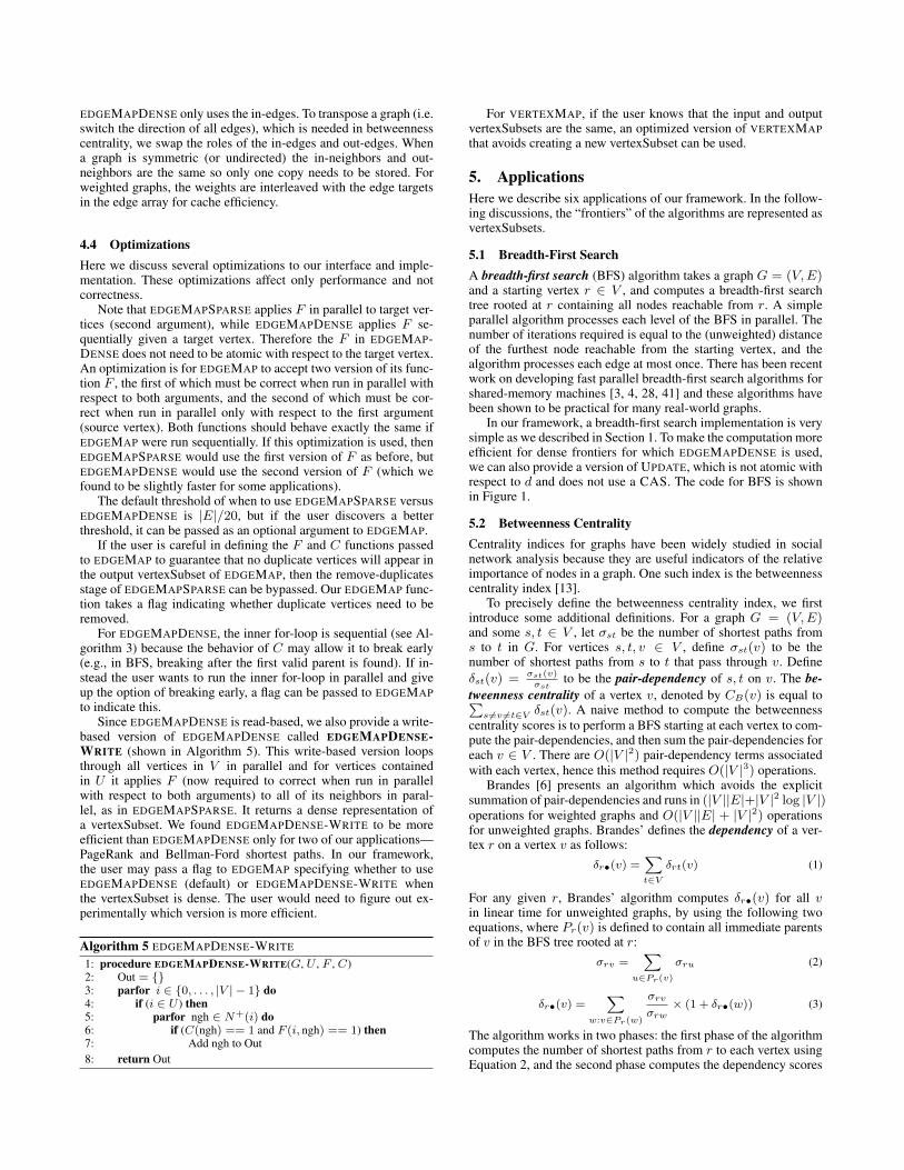
1: Parents = {−1, . . . ,−1} . initialized to all -1’s2:3: procedure UPDATE(s, d)4: return (CAS(&Parents[d], −1 , s ))5:6: procedure COND(i)7: return (Parents[i] == −1)8:9: procedure BFS(G, r) . r is the root
10: Parents[r] = r11: Frontier = {r} . vertexSubset initialized to contain only r12: while (SIZE(Frontier) 6= 0) do13: Frontier = EDGEMAP(G, Frontier,UPDATE, COND)
Figure 1. Pseudocode for Breadth-First Search in our framework.The compare-and-swap function CAS(loc,oldV,newV) atomicallychecks if the value at location loc is equal to oldV and if so itupdates loc with newV and returns true. Otherwise it leaves locunmodified and returns false.
we could compare with, and typically faster even on absolute termsto the largest systems run, which sometimes have two orders ofmagnitude more cores. Finally, commodity shared memory serversare quite reliable, often running for up to months or possibly yearswithout a failure.
Ligra supports two data types, one representing a graph G =(V,E) with vertices V and edges E, and another for represent-ing subsets of the vertices V , which we refer to as vertexSub-sets. Other than constructors and size queries, the interface suppliesonly two functions, one for mapping over vertices (VERTEXMAP)and the other for mapping over edges (EDGEMAP). Since a ver-texSubset is a subset of V , the VERTEXMAP can be used to mapover any subset of the original vertices, and hence its utility intraversal algorithms—or more generally in any algorithm in whichonly (possibly small) subsets of the graph are processed on eachround. The EDGEMAP also processes a subset of the edges, whichis specified using a vertexSubset to indicate the valid sources, anda Boolean function to indicate the valid targets of each edge. Ab-stractly, a vertexSubset is simply a set of integer labels for the in-cluded vertices and the VERTEXMAP simply applies the user sup-plied function to each integer. It is up to the user to maintain anyvertex based data. The implementation switches between a sparseand dense representation of the integers depending on the size ofthe vertexSubset. In our interface, multiple vertexSubsets can bemaintained and furthermore, a vertexSubset can be used for multi-ple graphs with different edge sets, as long as the number of verticesin the graphs are the same.
With this interface a breadth-first search (BFS), for example,can be implemented as shown in Figure 1. This version of BFSuses a Parents array (initialized all to −1, except for the root rwhere Parents[r] = r) in which each vertex will point to its parentin a BFS tree. As with standard parallel versions of BFS [28, 41],on each step i (starting at 0) the algorithm maintains a frontier of allvertices reachable from the root r in i steps. Initially a vertexSubsetcontaining just the root vertex is created to represent the frontier(line 11). Using EDGEMAP, each step checks the neighbors of thefrontier to see which have not been visited, updates those to point totheir parent in the frontier, and adds them to the next frontier (line13). The user supplied function UPDATE (lines 3–4) atomicallychecks to see if a vertex has been visited using a compare and swap(CAS) and returns true if not previously visited (Parents[i] ==−1). The COND function (lines 6–7) tells EDGEMAP to consideronly target vertices which have not been visited (here, this is notneeded for correctness, but is used for efficiency). The EDGEMAPfunction returns a new vertex set containing the target vertices forwhich UPDATE returns true, i.e., all the vertices in the next frontier
(line 13). The BFS completes when the frontier is empty and henceno more vertices are reachable.
The interface is designed to allow the edges to be processed indifferent orders depending on the particular situation. This is dif-ferent from many of the interfaces mentioned in the first paragraph(e.g. Pregel, GraphLab, GPS and Giraph) which are vertex basedand have the user hardcode how to loop over the out-edges or in-edges. Our implementation supports a few different ways to tra-verse the edges. One way is to loop over each vertex in a sparserepresentation of the active source vertices applying the functionto each out-edge (this is basically the order Pregel, GPS and Gi-raph supports). This loop over the out-edges can either be parallelor sequential depending on the degree of the vertex (Pregel and theothers do not support parallel looping over out-edges, although themost recent version of GraphLab does [17]). A dense representa-tion of the set of source vertices could also be used. Another wayto map over the edges is to loop over all destination vertices se-quentially or in parallel, and for each in-edge check if the source isin the source vertex set and apply the edge function if so. Finally,we can simply apply a flat map over all edges checking which needto be applied.
In this paper, we apply the Ligra framework to a collectionof problems: breadth-first search, betweenness centrality, graphradii estimation, graph-connectivity, PageRank, and Bellman-Fordsingle-source shortest paths. All of these applications have theproperty that they work in rounds and each round potentially pro-cesses only a subset of the vertices. In the case of BFS, each vertexis only processed once but in the others they can be processed mul-tiple times. For example, in the shortest paths algorithm a vertexonly needs to be added to the active vertex set if its distance haschanged. Similarly in a variant of PageRank, a vertex needs to beprocessed only if its PageRank value has changed by more thansome delta since it was last processed.
Betweenness centrality, a technique for measuring the “impor-tance” of vertices in a graph, is basically a version of BFS thataccumulates statistics along the way and propagates first in the for-ward direction and then backward direction. In betweenness cen-trality, one needs to keep around the frontiers during the forwardtraversal to facilitate the backward traversal. In Ligra, this is easilydone by storing the vertexSubsets in each iteration during the for-ward traversal. In contrast, this cannot be easily expressed in Pregeland GraphLab, because although vertices can be made inactive inPregel and GraphLab, the state is associated with the vertices asopposed to being separate.
Our contributions are threefold:
1. We provide an abstraction based on edgeMaps, vertexMapsand vertexSubsets for programming a class of parallel graphalgorithms.
2. We provide an efficient and lightweight implementation of ourframework, and applications using the framework.
3. We provide experimental evaluation of using the framework andtiming results of our applications on various input graphs.
The Ligra code and applications can be found at www.cs.cmu.edu/˜jshun/ligra/.
2. Related WorkBeamer et. al [3, 4] recently developed a very fast BFS for shared-memory machines.They use a hybrid BFS consisting of the conven-tional top-down approach, where each vertex on the current fron-tier explores all of its neighbors and adds unvisited neighbors tothe next frontier (write-based), and a bottom-up approach, whereeach unvisited vertex in the graph tries to find any parent (visitedvertex) among its neighbors (read-based). While the neighbor vis-

its in the top-down approach will mostly be to unvisited verticeswhen the frontier is small, for large frontiers many of the edgeswill be to neighbors already visited. The edges to visited neigh-bors can be avoided in the bottom-up approach because an unvis-ited vertex can stop checking once it has found a parent; this makesit more efficient than the top-down approach for large frontiers. Thedisadvantage of the bottom-up approach is that it processes all ofthe vertices, so is more expensive than the top-down approach forsmall frontiers. Beamer et. al.’s hybrid BFS switches between thetwo approaches based on the size of the frontier, and the represen-tation of the active set of vertices also switches between sparse anddense accordingly. They show that for small-world and scale-freegraphs, the hybrid BFS achieves a significant speedup over previ-ous BFS implementations based on the top-down approach. We usethis same idea in a more general setting.
Pegasus [24] and the Knowledge Discovery Toolbox (KDT)[15, 31] process graphs by using sparse matrix operations withgeneralized matrix operations. Each row/column corresponds to avertex and each non-zero in the matrix represents an edge. Pegasususes the Hadoop implementation of MapReduce in the distributed-computing setting, and includes implementations for PageRank,random walk with restart, graph diameter/radii, and connectedcomponents. It does not allow a sparse representation of the ver-tices and therefore is inefficient when only a small subset of ver-tices are active. Also, because it is built on top of MapReduce, itis hard to make it perform well. KDT provides a set of generalizedmatrix-vector building blocks for graph computations. It is built ontop of the the Combinatorial BLAS [8], a lower-level generalizedsparse matrix library for the distributed setting. Using the buildingblocks, the KDT developers implement algorithms for breadth-firstsearch, betweenness centrality, PageRank, belief propagation andMarkov Clustering. Since the abstraction allows for sparse vectorsas well as sparse matrices, it is suited for the case when only a smallnumber of vertices are active. However, it does not switch repre-sentations of the vertex sets based on its density. We give someperformance comparisons with both systems in Section 6.
Pregel is an API for processing large graphs in the distributedsetting [34]. It is a vertex-centric framework, where vertices canloop over their edges and send messages to all their out-neighbors.These messages are then collected at the target vertex, possibly us-ing associative combining. The system is bulk-synchronous so thereceived value is not seen until the next round. The reported per-formance of Pregel is relatively slow, likely due to the overhead ofthe framework and the use of a distributed memory machine. TheGPS [40] and Giraph [16] systems are public source implemen-tations of the Pregel interface with some additional features. TheGPS system allows for graph partitioning and reallocation duringthe computation. This improves performance over Pregel, but onlymarginally.
GraphLab is a framework for asynchronous parallel graph com-putations in machine learning. It works in both shared-memory anddistributed-memory architectures [29, 30]. It differs from Pregel inthat it does not work in bulk-synchronous steps, but rather allowsthe vertices to be processed asynchronously based on a sched-uler. The vertex functions can run at any time as long as specifiedconsistency rules are obeyed. It is therefore well-suited for themachine learning types of applications for which it is defined,where each vertex accumulates information from its neighborsstates and updates its state, possibly asynchronously. The recentPowerGraph framework combines the shared-memory and asyn-chronous properties of GraphLab with the associative combiningconcept of Pregel [17]. In contrast to our vertexSubset data type,both Pregel and GraphLab assume a single graph, and do not allowfor multiple vertex sets, since state is associated with the vertices.
Grace is a graph management system for shared-memory [39].It uses graph partitioning techniques and batched updates to ex-ploit locality. Updates to the graph are done transactionally. Theirreported times are slower than that of our system for applicationslike BFS and PageRank, after accounting for differences in inputsize and machine specifications.
GraphChi is a system for handling graph computations usingjust a PC [26]. It uses a novel parallel sliding windows methodfor processing graphs from disk. Although their running times areslower than ours, their system is designed for processing graphs outof memory, whereas we assume the graphs fit in memory.
Galois is a graph system for shared-memory based on set itera-tors [38]. Unlike our EDGEMAP and VERTEXMAP functions, theirset iterator does not abstract the internal details of the loop from theuser. Their sets of active elements for each iteration must be gener-ated directly by the user, unlike our EDGEMAP which generates avertexSubset which can be used for the next iteration.
Green-Marl is a domain-specific language for writing graph al-gorithms for shared-memory [21]. Graph traversal algorithms us-ing Green-Marl are written using built-in breadth-first search (BFS)and depth-first search (DFS) primitives whose implementations arebuilt into the compiler. Their language does not support operationsover arbitrary sets of vertices on each iteration of the traversal,and instead the user must explicitly filter out the vertices to skip.This makes it less flexible than our framework, which can operateon arbitrary vertexSubsets. In Green-Marl, for traversal algorithmswhich cannot be expressed using a BFS or DFS (e.g. radii estima-tion and Bellman-Ford shortest paths), the user has to write the for-loops themselves. On the other hand, such algorithms are naturallyexpressed in our framework.
Other high-performance libraries for parallel graph computa-tions include the Parallel Boost Graph Library (PBGL) [19] andthe Multithreaded Graph Library (MTGL) [5]. The former is devel-oped for the distributed-memory setting and the latter is developedfor massively multithreaded architectures. These libraries providefew higher-level abstractions beyond the graphs themselves.
3. PreliminariesA variable var with type type is denoted as var : type. We denote afunction f by f : X 7→ Y if each x ∈ X has a unique value y ∈ Ysuch that f(x) = y. We denote the Cartesian product of sets A andB by A × B where A × B = {(a, b) : a ∈ A ∧ b ∈ B}. Wedefine the Boolean value set bool to be the set {0, 1} (equivalently{false,true}).
We denote a directed unweighted graph by G = (V,E) whereV is the set of vertices and E is the set of (directed) edges in thegraph. Graphs have type graph, vertices have type vertex and edgeshave type vertex × vertex, where the first vertex is the source ofthe edge and the second the target. We will use the convention ofdenoting the number of vertices in a graph by |V | and number ofedges in a graph by |E|. We denote a weighted graph by G =(V,E,w), wherew is a function which maps an edge to a real value(w : vertex× vertex 7→ R), and each edge e ∈ E is associated withthe weight w(e). N+(v) denotes the set of out-neighbors of vertexv in G and deg+(v) denotes the out-degree of v in G. Similarly,N−(v) and deg−(v) denote the in-neighbors and in-degree of v inG.
A compare-and-swap (CAS) is an atomic instruction that takesthree arguments—a memory location (loc), an old value (oldV) anda new value (newV); if the value stored at loc is equal to oldVit atomically stores newV at loc and returns true, and otherwiseit does not modify loc and returns false. In our implementations,we use CAS’s both directly and as a subroutine to other atomicfunctions, such an as atomic increment. Throughout the paper weuse the notation &x to refer to the memory location of variable x.

4. Framework4.1 InterfaceFor an unweighted graph G = (V,E) or weighted graph G =(V,E,w(E)), our framework provides a vertexSubset type, whichrepresents a subset of vertices U ⊆ V . Note that V , and hence U ,may be shared among graphs with different edge sets. Except forsome constructor functions and some optional arguments describedin Section 4.4, the following describes our interface.
1. SIZE(U : vertexSubset) : N.Returns |U |.
2. EDGEMAP(G : graph,U : vertexSubset,F : (vertex × vertex) 7→ bool,C : vertex 7→ bool) : vertexSubset.
For an unweighted graph G = (V,E) EDGEMAP applies thefunction F to all edges with source vertex inU and target vertexsatisfying C. More precisely, for an active edge set
Ea = {(u, v) ∈ E | u ∈ U ∧ C(v) = true},F is applied to each element in Ea, and the return value ofEDGEMAP is a vertexSubset:
Out = {v | (u, v) ∈ Ea ∧ F (u, v) = true}.In this framework, F can run in parallel, so the user must ensureparallel correctness. F is allowed to side effect any data that it isassociated with (and does so when used in the graph algorithmswe discuss later), so F , C, Ea and Out can depend on order.The function C is useful in algorithms where a value associatedwith a vertex only needs to be updated once (i.e. breadth-firstsearch). If the user does not need the this functionality, a defaultfunction Ctrue which always returns true may be supplied.For weighted graphs, F takes the edge weight as an additionalargument.
3. VERTEXMAP(U : vertexSubset,F : vertex 7→ bool) : vertexSubset.
Applies F to every vertex in U . Its returns a vertexSubset:
Out = {u ∈ U | F (u) = true}As with EDGEMAP, the function F can run in parallel.
4.2 ImplementationWe index the vertices V of a graph from 0 to |V |−1. A vertexSub-set U ⊂ V is therefore a set of integers in the range 0, . . . , |V |−1.In our implementation this set is either represented sparsely as anarray of |U | integers (not necessarily sorted) or as a Boolean arrayof length |V |, true in location i if and only if i ∈ U . For exam-ple, for a graph with 8 vertices the sparse representation of a vertexsubset {0, 2, 3} could be [0, 2, 3] or [3, 0, 2] and the correspondingdense representation would be [1, 0, 1, 1, 0, 0, 0, 0]. The implemen-tation of vertexSubset contains routines for converting its sparserepresentation to a dense representation and vice versa. In the fol-lowing pseudocode we assume unweighted graphs, but it can easilybe extended to weighted graphs. Also we overload notation and useU and Out both to denote subsets of vertices and also to denote thevertexSubsets representing them.
For a given graphG = (V,E), a vertexSubset representing a setof vertices U ⊆ V and functions F and C, the EDGEMAP function(pseudocode shown in Algorithm 1) calls one of EDGEMAPSPARSE(Algorithm 2) and EDGEMAPDENSE (Algorithm 3) based on |U |and the number of outgoing edges of U (if this quantity is greaterthan some threshold, it calls EDGEMAPDENSE, and otherwise itcalls EDGEMAPSPARSE). EDGEMAPSPARSE loops through all
vertices present in U in parallel and for a given u ∈ U appliesF (u, ngh) to all of u’s neighbors ngh in G in parallel. It returnsa vertexSubset that is represented sparsely. The work performedby EDGEMAPSPARSE is proportional to |U | plus the sum of theout-degrees of U . On the other hand, EDGEMAPDENSE loopsthrough all vertices in V in parallel and for each vertex v ∈ Vit sequentially applies the function F (ngh, v) for each of v’s neigh-bors ngh that are in U , until C(u) returns false. It returns a denserepresentation of a vertexSubset. For EDGEMAPSPARSE, since asparse representation of a vertexSubset is returned, duplicate ver-tex IDs in the output vertexSubset must be removed. IntuitivelyEDGEMAPSPARSE should be more efficient than EDGEMAP-DENSE for small vertexSubsets, while for larger vertexSubsetsEDGEMAPDENSE should be faster. The threshold of when touse EDGEMAPSPARSE versus EDGEMAPDENSE is set to |E|/20,which we found to work well across all of our applications.
Algorithm 1 EDGEMAP
1: procedure EDGEMAP(G, U , F , C)2: if (|U | + sum of out-degrees of U > threshold) then3: return EDGEMAPDENSE(G, U , F , C)4: else return EDGEMAPSPARSE(G, U , F , C)
Algorithm 2 EDGEMAPSPARSE
1: procedure EDGEMAPSPARSE(G, U , F , C)2: Out = {}3: parfor each v ∈ U do4: parfor ngh ∈ N+(v) do5: if (C(ngh) == 1 and F (v, ngh) == 1) then6: Add ngh to Out7: Remove duplicates from Out8: return Out
Algorithm 3 EDGEMAPDENSE
1: procedure EDGEMAPDENSE(G, U , F , C)2: Out = {}3: parfor i ∈ {0, . . . , |V | − 1} do4: if (C(i) == 1) then5: for ngh ∈ N−(i) do6: if (ngh ∈ U and F (ngh, i) == 1) then7: Add i to Out8: if (C(i) == 0) then break9: return Out
The VERTEXMAP function (Algorithm 4) takes as inputs avertexSubset representing the vertices U and a Boolean functionF , and applies F to all vertices in U . It returns a vertexSubsetrepresenting subset Out ⊆ U containing vertices u such that F (u)returns true.
Algorithm 4 VERTEXMAP
1: procedure VERTEXMAP(U , F )2: Out = {}3: parfor u ∈ U do4: if (F (u) == 1) then Add u to Out5: return Out
4.3 Graph RepresentationOur code represents in-edges and out-edges as arrays. In particularthe in-edges for all vertices are kept in one array partitioned bytheir target vertex and storing the source vertices. Similarly, the out-edges are in an array partitioned by the source vertices and storingthe target vertices. Each vertex points to the start of their in-edgeand out-edge partitions and also maintains their in-degree and out-degree. Note that EDGEMAPSPARSE only uses the out-edges and
EDGEMAPDENSE only uses the in-edges. To transpose a graph (i.e.switch the direction of all edges), which is needed in betweennesscentrality, we swap the roles of the in-edges and out-edges. Whena graph is symmetric (or undirected) the in-neighbors and out-neighbors are the same so only one copy needs to be stored. Forweighted graphs, the weights are interleaved with the edge targetsin the edge array for cache efficiency.
4.4 OptimizationsHere we discuss several optimizations to our interface and imple-mentation. These optimizations affect only performance and notcorrectness.
Note that EDGEMAPSPARSE applies F in parallel to target ver-tices (second argument), while EDGEMAPDENSE applies F se-quentially given a target vertex. Therefore the F in EDGEMAP-DENSE does not need to be atomic with respect to the target vertex.An optimization is for EDGEMAP to accept two version of its func-tion F , the first of which must be correct when run in parallel withrespect to both arguments, and the second of which must be cor-rect when run in parallel only with respect to the first argument(source vertex). Both functions should behave exactly the same ifEDGEMAP were run sequentially. If this optimization is used, thenEDGEMAPSPARSE would use the first version of F as before, butEDGEMAPDENSE would use the second version of F (which wefound to be slightly faster for some applications).
The default threshold of when to use EDGEMAPSPARSE versusEDGEMAPDENSE is |E|/20, but if the user discovers a betterthreshold, it can be passed as an optional argument to EDGEMAP.
If the user is careful in defining the F and C functions passedto EDGEMAP to guarantee that no duplicate vertices will appear inthe output vertexSubset of EDGEMAP, then the remove-duplicatesstage of EDGEMAPSPARSE can be bypassed. Our EDGEMAP func-tion takes a flag indicating whether duplicate vertices need to beremoved.
For EDGEMAPDENSE, the inner for-loop is sequential (see Al-gorithm 3) because the behavior of C may allow it to break early(e.g., in BFS, breaking after the first valid parent is found). If in-stead the user wants to run the inner for-loop in parallel and giveup the option of breaking early, a flag can be passed to EDGEMAPto indicate this.
Since EDGEMAPDENSE is read-based, we also provide a write-based version of EDGEMAPDENSE called EDGEMAPDENSE-WRITE (shown in Algorithm 5). This write-based version loopsthrough all vertices in V in parallel and for vertices containedin U it applies F (now required to correct when run in parallelwith respect to both arguments) to all of its neighbors in paral-lel, as in EDGEMAPSPARSE. It returns a dense representation ofa vertexSubset. We found EDGEMAPDENSE-WRITE to be moreefficient than EDGEMAPDENSE only for two of our applications—PageRank and Bellman-Ford shortest paths. In our framework,the user may pass a flag to EDGEMAP specifying whether to useEDGEMAPDENSE (default) or EDGEMAPDENSE-WRITE whenthe vertexSubset is dense. The user would need to figure out ex-perimentally which version is more efficient.
Algorithm 5 EDGEMAPDENSE-WRITE
1: procedure EDGEMAPDENSE-WRITE(G, U , F , C)2: Out = {}3: parfor i ∈ {0, . . . , |V | − 1} do4: if (i ∈ U ) then5: parfor ngh ∈ N+(i) do6: if (C(ngh) == 1 and F (i, ngh) == 1) then7: Add ngh to Out8: return Out
For VERTEXMAP, if the user knows that the input and outputvertexSubsets are the same, an optimized version of VERTEXMAPthat avoids creating a new vertexSubset can be used.
5. ApplicationsHere we describe six applications of our framework. In the follow-ing discussions, the “frontiers” of the algorithms are represented asvertexSubsets.
5.1 Breadth-First SearchA breadth-first search (BFS) algorithm takes a graph G = (V,E)and a starting vertex r ∈ V , and computes a breadth-first searchtree rooted at r containing all nodes reachable from r. A simpleparallel algorithm processes each level of the BFS in parallel. Thenumber of iterations required is equal to the (unweighted) distanceof the furthest node reachable from the starting vertex, and thealgorithm processes each edge at most once. There has been recentwork on developing fast parallel breadth-first search algorithms forshared-memory machines [3, 4, 28, 41] and these algorithms havebeen shown to be practical for many real-world graphs.
In our framework, a breadth-first search implementation is verysimple as we described in Section 1. To make the computation moreefficient for dense frontiers for which EDGEMAPDENSE is used,we can also provide a version of UPDATE, which is not atomic withrespect to d and does not use a CAS. The code for BFS is shownin Figure 1.
5.2 Betweenness CentralityCentrality indices for graphs have been widely studied in socialnetwork analysis because they are useful indicators of the relativeimportance of nodes in a graph. One such index is the betweennesscentrality index [13].
To precisely define the betweenness centrality index, we firstintroduce some additional definitions. For a graph G = (V,E)and some s, t ∈ V , let σst be the number of shortest paths froms to t in G. For vertices s, t, v ∈ V , define σst(v) to be thenumber of shortest paths from s to t that pass through v. Defineδst(v) = σst(v)
σstto be the pair-dependency of s, t on v. The be-
tweenness centrality of a vertex v, denoted by CB(v) is equal to∑s 6=v 6=t∈V δst(v). A naive method to compute the betweenness
centrality scores is to perform a BFS starting at each vertex to com-pute the pair-dependencies, and then sum the pair-dependencies foreach v ∈ V . There are O(|V |2) pair-dependency terms associatedwith each vertex, hence this method requires O(|V |3) operations.
Brandes [6] presents an algorithm which avoids the explicitsummation of pair-dependencies and runs in (|V ||E|+|V |2 log |V |)operations for weighted graphs and O(|V ||E| + |V |2) operationsfor unweighted graphs. Brandes’ defines the dependency of a ver-tex r on a vertex v as follows:
δr•(v) =∑t∈V
δrt(v) (1)
For any given r, Brandes’ algorithm computes δr•(v) for all vin linear time for unweighted graphs, by using the following twoequations, where Pr(v) is defined to contain all immediate parentsof v in the BFS tree rooted at r:
σrv =∑
u∈Pr(v)
σru (2)
δr•(v) =∑
w:v∈Pr(w)
σrv
σrw× (1 + δr•(w)) (3)
The algorithm works in two phases: the first phase of the algorithmcomputes the number of shortest paths from r to each vertex usingEquation 2, and the second phase computes the dependency scores

via Equation 3. The first phase is similar to a forward BFS fromvertex r and the second phase works backwards from the last fron-tier of the BFS. This algorithm can be parallelized in two way—(1)for each vertex, the traversal can be done in parallel, and (2) eachvertex can perform their individual computations independently inparallel with other vertices’ computations. Although much more ef-ficient than the naive algorithm, Brandes’ algorithm still requires atleast quadratic time, and is thus prohibitive for large graphs. To ad-dress this problem, there has been work on computing approximatebetweenness centrality scores based on using the pair-dependencycontributions from just a sample of the vertices of the vertices andscaling the betweenness centrality scores appropriately [2, 14]. TheKDT package provides a parallel implementation of batched com-putation of betweenness centrality scores by running multiple indi-vidual computations independently in parallel [31].
We describe the betweenness centrality computation from asingle root vertex—these computations can be run independentlyin parallel for any sample of the vertices. The computation hereis different from the BFS described in Section 5.1 in that insteadof finding a parent, each vertex v needs to maintain a count of thenumber of shortest paths passing through it. This means the numberof updates to v is equal to its number of parents in the BFS tree,instead of just one update as in BFS.
The psuedocode for our implementation is shown in Algorithm6. The frontier is initialized to contain just r. For the first phasewe use an array of integers NumPaths, which is initialized to all0’s except for the root vertex which has NumPaths[r] set to 1.By traversing the graph in a breadth-first manner and updating theNumPaths value for each v that is traversed, we obtain the numberof shortest paths passing through each v from r (NumPaths[v]will remain 0 if v is unreachable from r). The PATHSUPDATEfunction passed to EDGEMAP is shown in lines 13–18. As there canbe multiple updates to some NumPaths[v] in parallel, the updateattempt is repeated with a compare-and-swap until successful. Line18 guarantees that a vertex is placed on the frontier only once, sincethe old NumPaths value will be 0 for at most one update. Eachfrontier of the search is stored in a Levels array for use in the secondphase.
To keep track of vertices that have been visited (and avoid hav-ing to remove duplicates in EDGEMAPSPARSE), we also maintaina Boolean array Visited. Visited is initialized to all 0’s (except forthe root vertex whose entry is set to 1), and we set a vertex’s en-try in Visited to 1 after it is first visited in the computation. To dothis, we use a VERTEXMAP and pass the VISIT function shown inlines 9–11 of Algorithm 6 to VERTEXMAP. The COND function inlines 27–28 makes EDGEMAP only consider unvisited target ver-tices. The psuedocode for the first phase starting at a root vertex isshown in lines 32 to 36.
For the second phase, we use a new array Dependencies (ini-tialized to all 0.0) and reuse the Visited array (reinitialized to all0). Also we transpose the graph (line 40), since edges now need topoint in the reverse direction. The algorithm operates on the ver-texSubsets in the Levels array returned from the first phase in re-verse order, uses the same VISIT and COND functions as in the firstphase, and passes the DEPUPDATE function shown in lines 20 to25 of Algorithm 6 to EDGEMAP. Psuedocode for the second phaseof the betweenness-centrality computation is shown in lines 42–46.
5.3 Graph Radii Estimation and Multiple BFSFor a graphG = (V,E), the radius of a node v ∈ V is the shortestdistance to the furthest reachable node of v. The diameter of thegraph is the maximum radius over all v ∈ V . For unweightedgraphs, one simple method for computing the radii of all nodes (andhence the diameter of the graph) is to run |V | BFS’s, one starting ateach vertex. However, for large graphs this method is impractical
Algorithm 6 Betweenness Centrality1: NumPaths = {0, . . . , 0} . initialized to all 02: Visited = {0, . . . , 0} . initialized to all 03: NumPaths[r] = 14: Visited[r] = 15: currLevel = 06: Levels = [ ]7: Dependencies = {0.0, . . . , 0.0} . initialized to all 0.08:9: procedure VISIT(i)
10: Visited[i] = 111: return 112:13: procedure PATHSUPDATE(s, d)14: repeat15: oldV = NumPaths[d]16: newV = oldV + NumPaths[s]17: until (CAS(&NumPaths[d], oldV, newV) == 1)18: return (oldV == 0)19:20: procedure DEPUPDATE(s, d)21: repeat22: oldV = Dependencies[d]
23: newV = oldV +NumPaths[d]NumPaths[s] × (1 + Dependencies[s])
24: until (CAS(&Dependencies[d], oldV, newV) == 1)25: return (oldV == 0.0)26:27: procedure COND(i)28: return (Visited[i] == 0)29:30: procedure BC(G, r)31: Frontier = {r} . vertexSubset initialized to contain only r32: while (SIZE(Frontier) 6= 0) do . Phase 133: Frontier = EDGEMAP(G, Frontier, PATHSUPDATE, COND)34: Levels[currLevel] = Frontier35: Frontier = VERTEXMAP(Frontier,VISIT)36: currLevel = currLevel + 137:38: Visited = {0, . . . , 0} . reinitialize to all 039: currLevel = currLevel− 140: TRANSPOSE(G) . transpose graph41:42: while (currLevel ≥ 0) do . Phase 243: Frontier = Levels[currLevel]44: VERTEXMAP(Frontier,VISIT)45: EDGEMAP(G, Frontier,DEPUPDATE, COND)46: currLevel = currLevel− 147: return Dependencies
as each BFS requires O(|V | + |E|) operations, leading to a totalof O(|V |2 + |V ||E|) operations (see [11]). This approach can beparallelized by running the BFS’s independently in parallel, andalso by parallelizing each individual BFS, but currently this is stillimpractical for large graphs.
There has been work on techniques to estimate the diameter ofa graph. Magnien et. al. [33] describe several techniques for com-puting upper and lower bounds on the diameter of a graph, usingBFS’s and spanning subgraphs. They describe a method called thedouble sweep lower bound, which works by first running a BFSfrom some node v and then a second BFS from the furthest nodefrom v (call it w). The radius of w is then taken to be a lowerbound on the diameter of the graph. Their method can be repeatedby picking more vertices to run BFS’s from. Ferrez et. al. [12] per-form experiments with parallel implementations of some of thesemethods. Another approach based on counting neighborhood sizeswas described by Palmer et. al. [37]. Their algorithm approximatesthe neighborhood function for each vertex in a graph, which is moregeneral than computing graph radii. Kang et. al. [23] parallelize this

algorithm using MapReduce. Cohen [10] describes an algorithm forapproximating neighborhood sizes, which requires O(|E| log |V |)expected number of operations for undirected graphs.
We implement the simple method for estimating graph radii byperforming BFS’s from a sample of K vertices. Its accuracy canbe improved by using the double sweep method of Magnien et. al.[33]. Instead of running the BFS’s in parallel independently, werun multiple BFS’s together. In the multiple-BFS algorithm, eachvertex maintains a bit-vector of length K. Initially K vertices arechosen randomly to act as “source” vertices and each of these Kvertices has exactly one unique bit in their bit-vector set to 1; allother vertices have their bit-vectors initialized to all 0’s. The Ksampled vertices are placed on the initial frontier of the multiple-BFS search. In each iteration, each frontier vertex bitwise-ORsits vector into each of its neighbors’ vectors. Vertices whose bit-vectors changed in an iteration are placed on the frontier for thenext iteration. The algorithm iterates until none of the bit-vectorschange.
For a sample of size K this algorithm simulates running KBFS’s in parallel, but without computing the BFS tree (which isnot needed for the radii computation). Storing the iteration numberin which a vertex v’s bit-vector last changed is a lower-bound onthe radius of v since at least one of the K sampled vertices tookthis many rounds to reach v. If K is set to be the number of bits ina word (32 or 64) this algorithm is more efficient than naively per-forming K individual BFS’s in two ways: (1) the frontiers of theK BFS’s could overlap in any given iteration and this algorithmstores the union of these frontiers usually leading to fewer edgestraversed per iteration and (2) performing a bitwise-OR on bit-vectors can pass information from more than one of the K BFS’swhile only requiring one arithmetic operation. Note that this algo-rithm only estimates the diameter of the connected components ofthe graph which contain at least one of the K sampled vertices; ifthere are multiple connected components in the graph, one wouldfirst compute in parallel the components of the graph and then runthe multiple-BFS algorithm in parallel on each component.
To implement the multiple-BFS algorithm in our framework(pseudocode shown in Algorithm 7), we maintain two bit-vectors,Visited and NextVisited, which are initialized to all 0’s, except forthe K sampled vertices each of which has a unique bit in theirVisited bit-vector set to 1. We also maintain an array Radii, whichfor each vertex stores the iteration number in which the bit-vectorof the vertex last changed. It is initialized to all ∞ except for theK sampled vertices which have a Radii entry of 0. At the end ofthe algorithm, Radii contains the estimated (lower-bound) radius ofeach vertex, the maximum of which is a lower-bound on the graphdiameter. In the pseudocode, we use “|” to denote the bitwise-ORoperation. The initial frontier contains theK sampled vertices. Theupdate function RADIIUPDATE passed to EDGEMAP is shown inlines 6–12 of Algorithm 7. ATOMICOR(x, y) performs a bitwise-OR of y with the value stored at x and atomically updates x withthis new value. It is implemented using a compare-and-swap. Thereason we have both Visited and NextVisited is so that new bitsthat a vertex receives in an iteration do not get propagated to itsneighbors in the same round, otherwise the values in Radii wouldbe incorrect. The compare-and-swap on line 11 guarantees that anyRadii entry is updated at most once (and returns true) per iteration.Therefore any vertex will be placed at most once on the nextfrontier, eliminating the need for removing duplicates. As in theother implementations, we can provide a version of RADIIUPDATEnon-atomic with respect to d to EDGEMAP.
The ORCOPY function (lines 14–16) passed to VERTEXMAPsimply takes an index i, performs a bitwise-OR of NextVisited[i]and Visited[i] and stores the result in NextVisited[i]. We use thisbecause the roles of NextVisited and Visited are switched between
iterations. The while loop in lines 22–26 is executed until theentries of the Radii array do not change (or equivalently, none ofthe bit-vectors change).
Algorithm 7 Radii Estimation1: Visited = {0, . . . , 0} . initialized to all 02: NextVisited = {0, . . . , 0} . initialized to all 03: Radii = {∞, . . . ,∞} . initialized to all∞4: round = 05:6: procedure RADIIUPDATE(s, d)7: if (Visited[d] 6= Visited[s]) then8: ATOMICOR(&NextVisited[d],Visited[d] | Visited[s])9: oldRadii = Radii[d]
10: if (Radii[d] 6= round) then11: return CAS(&Radii[d], oldRadii, round)
12: return 013:14: procedure ORCOPY(i)15: NextVisited[i] = NextVisited[i] | Visited[i]16: return 117:18: procedure RADII(G)19: Sample K vertices and for each one set a unique bit in Visited to 120: Initialize Frontier to contain the K sampled vertices21: Set the Radii entries of the sampled vertices to 022: while (SIZE(Frontier) 6= 0) do23: round = round + 124: Frontier = EDGEMAP(G, Frontier, RADIIUPDATE, Ctrue)25: Frontier = VERTEXMAP(Frontier,ORCOPY)26: SWAP(Visited,NextVisited) . switch roles of bit-vectors27: return Radii
5.4 Connected ComponentsFor an undirected graph G = (V,E), a connected componentC ⊆ V is one in which all vertices in C can reach one another.The connected components problem is to find C1, . . . , Ck suchthat each Ci is a connected component,
⋃i Ci = V , and there is
no path between vertices belonging to different components.One method of computing the connected components of a graph
is to maintain an array IDs of size |V | initialized such that IDs[i] =i, and iteratively have every vertex update its IDs entry to be theminimum IDs entry of all of its neighbors inG. The total number ofoperations performed by this algorithm isO(d(|V |+|E|)) where dis the diameter of G. For high-diameter graphs, this algorithm canperform much worse than standard edge-based algorithms whichrequire onlyO(|V |+|E|) operations [11, 22], but for low-diametergraphs it runs reasonably well. We show this algorithm as a simpleapplication of our framework.
The pseudocode for our implementation is shown in Algorithm8. The initial frontier contains all vertices in V . In addition tothe IDs array, we maintain a second array prevIDs (used to checkwhether a vertex has been placed on the frontier in a given iterationyet), and pass the CCUPDATE function shown in lines 4–8 ofAlgorithm 8 to EDGEMAP. WRITEMIN(x, y) atomically updatesthe value at location x to be the minimum of x’s old value andy, and is implemented with a compare-and-swap. It returns true ifthe value at location x was changed, and false otherwise. Line 7places a vertex on the next frontier if and only if its ID changed inthe iteration. To synchronize the values of prevIDs and IDs afterevery iteration, we pass the COPY function to VERTEXMAP. Thewhile loop in lines 16–18 is executed until IDs remains the sameas prevIDs. When the algorithm terminates, all vertices in the samecomponent will have the same value stored in their IDs entry.

Algorithm 8 Connected Components1: IDs = {0, . . . , |V | − 1} . initialized such that IDs[i] = i2: prevIDs = {0, . . . , |V | − 1} . initialized such that prevIDs[i] = i3:4: procedure CCUPDATE(s, d)5: origID = IDs[d]6: if (WRITEMIN(&IDs[d], IDs[s])) then7: return (origID == prevIDs[d])8: return 09:
10: procedure COPY(i)11: prevIDs[i] = IDs[i]12: return 113:14: procedure CC(G)15: Frontier = {0, . . . , |V | − 1} . vertexSubset initialized to V16: while (SIZE(Frontier) 6= 0) do17: Frontier = VERTEXMAP(Frontier, COPY)18: Frontier = EDGEMAP(G, Frontier, CCUPDATE, Ctrue)
19: return IDs
5.5 PageRankPageRank is an algorithm that was first used by Google to computethe relative importance of webpages [7]. It takes as input a graphG = (V,E), a damping factor 0 ≤ γ ≤ 1 and a convergenceconstant ε. It initializes a PageRank vector PR of length |V | tohave all entries set to 1
|V | , and iteratively applies the followingequation for all indices v, until the sum of the differences of PRvalues between iterations drops to below ε:
PR[v] =1− γ|V |
+ γ∑
u∈N−(v)
PR[u]
deg+(u)(4)
This leads to a very simple implementation in our framework.We also describe a variant of PageRank (PageRank-Delta) whichapplies Equation (4) to only a subset of V in an iteration. Bychoosing the subset to contain only vertices whose PageRank entrythat changed by more than a certain amount, we can speed up thecomputation.
The pseudocode for our implementation of PageRank is shownin Algorithm 9. In every iteration, the frontier contains all vertices.Our implementation maintains two arrays pcurr and pnext each oflength |V |. pcurr is initialized to 1
|V | for each entry and pnext is ini-tialized to all 0.0’s. The PRUPDATE function passed to EDGEMAPis shown in lines 5–7. ATOMICINCREMENT(x, y) atomically addsy to the value at location x and stores the result in location x; itcan be implemented with a compare-and-swap. Each iteration ofthe while loop (lines 18–22) applies an EDGEMAP, uses a VER-TEXMAP to process the result of the EDGEMAP, computes the er-ror for the iteration and switches the roles of pnext and pcurr. ThePRLOCALCOMPUTE function (lines 9–13) passed to VERTEXMAPnormalizes the result of the EDGEMAP by γ, adds a constant, com-putes the absolute difference between pnext and pcurr, and resets pcurr
to 0.0 for the next iteration (since the roles of pnext and pcurr becomeswitched). The while loop is executed until the error drops below ε.
PageRank-Delta is a variant of PageRank in which vertices areactive in an iteration only if they have accumulated enough changein their PR value. This idea is used in GraphLab for computingPageRank [30]. In our framework, in each EDGEMAP verticespass their changes (deltas) in PR value to their neighbors, andall vertices accumulate a sum of delta contributions from theirneighbors. Each VERTEXMAP only updates and returns verticeswhose accumulated delta contributions from neighbors is more thana δ-fraction of its PR value since the last time it was active. Suchan implementation allows for vertices which do not influence thePR values much to stay inactive, thereby shrinking the frontier. We
Algorithm 9 PageRank1: pcurr = { 1
|V | , . . . ,1|V |} . initialized to all 1
|V |2: pnext = {0.0, . . . , 0.0} . initialized to all 0.03: diff = {} . array to store differences4:5: procedure PRUPDATE(s, d)6: ATOMICINCREMENT(&pnext[d],
pcurr[s]
deg+(s))
7: return 18:9: procedure PRLOCALCOMPUTE(i)
10: pnext[i] = (γ × pnext[i]) + 1−γ|V |
11: diff[i] =∣∣pnext[i]− pcurr[i]
∣∣12: pcurr[i] = 0.013: return 114:15: procedure PAGERANK(G, γ, ε)16: Frontier = {0, . . . , |V | − 1} . vertexSubset initialized to V17: error =∞18: while (error > ε) do19: Frontier = EDGEMAP(G, Frontier, PRUPDATE, Ctrue)20: Frontier = VERTEXMAP(Frontier, PRLOCALCOMPUTE)21: error = sum of diff entries22: SWAP(pcurr, pnext)
23: return pcurr
can implement PageRank-Delta in our framework by modifying thefunction passed to EDGEMAP to pass the deltas instead of the PRvalues, and modifying the function passed to VERTEXMAP to onlyperform updates and return true for the vertices whose accumulateddelta contributions from neighbors since it was last active is morethan a δ-fraction of its PR value. Due to space limitations, we donot show the pseudocode for this algorithm.
5.6 Bellman-Ford Shortest PathsThe single-source shortest paths problem takes as input a weightedgraph G = (V,E,w(E)) and a root vertex r, and either computesthe shortest path distance from r to each vertex in V (if a vertex isunreachable from r, then the distance returned is∞), or reports theexistence of a negative cycle.
If the edge weights are all non-negative, then the single-sourceshortest paths problem can be solved with Dijkstra’s algorithm [11].Parallel variants of Dijkstra’s algorithm have been studied [36], andhave been shown to work well on real-world graphs [32]. However,Dijkstra’s algorithm does not work with negative edge weights,and the Bellman-Ford algorithm can be used instead in this case.Although in the worst case the Bellman-Ford algorithm requiresO(|V ||E|) operations, in contrast to the O(|E| + |V | log |V |)worst-case operations of Dijkstra’s algorithm, in practice it can re-quire many fewer than the worst case since on every step only someof the vertices might change distances. It is therefore important totake advantage of this fact and only process vertices when they ac-tually change distance.
We first describe the standard Bellman-Ford algorithm [11] andthen show how it can be implemented in our framework. Thealgorithm initializes the shortest paths array SP to all ∞ exceptfor the root vertex which has an entry of 0. A RELAX procedure isrepeatedly invoked by Bellman-Ford. RELAX takes G as an inputand checks for each edge (u, v) if SP[u] + w(u, v) < SP[v]; ifso, it sets SP[v] to SP[u] + w(u, v). If a call to RELAX does notchange any SP values then the algorithm terminates. If RELAX iscalled |V | or more times, then there is a negative cycle in G andthe Bellman-Ford algorithm reports the existence of one.
To implement the Bellman-Ford algorithm in our framework(pseudocode shown in Algorithm 10) we maintain a Visited arrayin addition to the SP array. Since only vertices whose SP value
has changed in an iteration need to propagate its SP value to itsneighbors, the Visited array (initialized to all 0’s) keeps track ofwhich vertices had their SP value changed in an iteration. Theupdate function passed to EDGEMAP is shown in lines 4–7 ofAlgorithm 10 (note that since this algorithm works on weightedgraphs, the update function has the edge weight as an additionalargument). It uses WRITEMIN (as described in Section 5.4) toposssibly update SP with a smaller path length. The compare-and-swap on line 6 guarantees that a vertex is placed on the frontier atmost once per iteration. The initial frontier contains just the rootvertex r. Each iteration of the while loop in lines 17–20 applies theEDGEMAP, which outputs a vertexSubset containing the verticeswhose SP value changed. In order to reset the Visited array afteran EDGEMAP, the BFRESET function (lines 9–11) is passed toVERTEXMAP. The algorithm either runs until no SP values changeor runs for |V | iterations and reports the existence of a negative-weight cycle. An iteration here differs from the RELAX procedurein that RELAX processes all vertices each time.
Algorithm 10 Bellman-Ford1: SP = {∞, . . . ,∞} . initialized to all∞2: Visited = {0, . . . , 0} . initialized to all 03:4: procedure BFUPDATE(s, d, edgeWeight)5: if (WRITEMIN(&SP[d], SP[s] + edgeWeight)) then6: return CAS(&Visited[d], 0, 1)7: else return 08:9: procedure BFRESET(i)
10: Visited[i] = 011: return 112:13: procedure BELLMAN-FORD(G, r)14: SP[r] = 015: Frontier = {r} . vertexSubset initialized to contain just r16: round = 017: while (SIZE(Frontier) 6= 0 and round < |V |) do18: round = round + 119: Frontier = EDGEMAP(G, Frontier, BF-UPDATE, Ctrue)20: Frontier = VERTEXMAP(Frontier, BF-RESET)
21: if (round == |V |) then return “negative-weight cycle”22: else return SP
6. ExperimentsAll of the experiments presented in this paper were performed on a40-core Intel machine (with hyper-threading) with 4×2.4GHz Intel10-core E7-8870 Xeon processors, a 1066MHz bus, and 256GB ofmain memory. The parallel programs were compiled with Intel’sicpc compiler (version 12.1.0) using CilkPlus [27] with the -O3flag. The sequential programs were compiled using g++ 4.4.1 withthe -O2 flag. We also ran experiments on a 64-core AMD Opteronmachine, but the results are slower than the ones from the Intelmachine so we only report the latter.
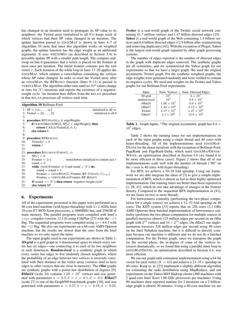
The input graphs used in our experiments are shown in Table 1.3D-grid is a grid graph in 3-dimensional space in which every ver-tex has six edges—one connecting it to each of its two neighborsin each dimension. Random-local is a synthetic graph in whichevery vertex has edges to five randomly chosen neighbors, wherethe probability of an edge between two vertices is inversely corre-lated with their distance in the vertex array (vertices tend to haveedges to other vertices that are close in memory). The rMat graphsare synthetic graphs with a power-law distribution of degrees [9].RMat24 (scale 24) contains 1.68 × 10⁷ vertices and was gener-ated with parameters a = 0.5, b = c = 0.1, d = 0.3. RMat27(scale 27) is one of the Graph500 benchmark graphs [18], and wasgenerated with parameters a = 0.57, b = c = 0.19, d = 0.05.
Twitter is a real-world graph of the Twitter social network con-taining 41.7 million vertices and 1.47 billion directed edges [25] .Yahoo is a real-world graph of the Web containing 1.4 billion ver-tices and 6.6 billion directed edges (12.9 billion after symmetrizingand removing duplicates) [42]. With the exception of Pregel, Yahoois the largest real-world graph reported by other graph processingsystems.
The number of edges reported is the number of directed edgesin the graph with duplicate edges removed. The synthetic graphsare all symmetric, and we symmetrized the Yahoo graph for ourexperiments so that we have a larger graph. We used the originalasymmetric Twitter graph. For the synthetic weighted graphs, theedge weights were generated randomly and were verified to containno negative cycles. We used unit weights on the Twitter and Yahoographs for our Bellman-Ford experiments.
Input Num. Vertices Num. Directed Edges3D-grid 107 6× 10⁷
random-local 107 9.8× 10⁷
rMat24 1.68× 10⁷ 9.9× 10⁷
rMat27 1.34× 10⁸ 2.12× 10⁹
Twitter 4.17× 10⁷ 1.47× 10⁹
Yahoo* 1.4× 10⁹ 12.9× 10⁹
Table 1. Graph inputs. *The original asymmetric graph has 6.6×10⁹ edges.
Table 2 shows the running times for our implementations oneach of the input graphs using a single thread and 40 cores withhyper-threading. All of the implementations used EDGEMAP-DENSE for the dense iterations with the exception of Bellman-Ford,PageRank and PageRank-Delta, which used EDGEMAPDENSE-WRITE, an optimization described in Section 4.4 (we found it tobe more efficient in these cases). Figure 2 shows that all of ourimplementations scale well with the number of threads (“80” onthe x-axis is 40 cores with hyper-threading).
For BFS, we achieve a 10–28 fold speedup. Using our frame-work we are able integrate the ideas of [3] to give a simple imple-mentation of BFS, which is almost as fast as their highly optimizedimplementation. Our running times are better than those reported in[1, 28, 41], which do not take advantage of changes in the frontierdensity. Compared to the sequential BFS implementation in [41],we are faster on two or more threads.
For betweenness centrality (performing the two-phase compu-tation for a single source) we achieve a 12–32 fold speedup on 40cores. The KDT system [31] reports that on 256 cores (2.1 GHzAMD Opteron) their batched implementation of betweenness cen-trality (performs the two-phase computation for multiple sources inparallel) traverses almost 125 million edges per second on an rMatgraph with 218 vertices and 16× 218 edges. On rMat27 our imple-mentation traverses 526 million edges per second using 40 coreson the Intel Nehalem machine, but it is difficult to directly com-pare because our machine is different and we do not do a batchedcomputation. For the Twitter graph, since we transpose the graphfor the second phase, the in-degree of some of the vertices in-creases dramatically, so we found that using a parallel inner loop inEDGEMAPDENSE, an optimization described in Section 4.4, wasmore efficient.
We ran our graph radii estimation implementation using a 64-bitvector for each vertex (K = 64) and achieve a 23–35× speedup on40 cores. Kang et. al. [23] implement a slightly different algorithmfor estimating the radii distribution using MapReduce, and runexperiments on the Yahoo M45 Hadoop cluster (480 machines with2 quad-core Intel Xeon 1.86 GHz processors per machine). Using90 machines their reported runtime for 3 iterations on a 2 billion-edge graph is almost 30 minutes. Using a 40-core machine we are

Application 3D-grid random-local rMat24 rMat27 Twitter Yahoo(1) (40h) (SU) (1) (40h) (SU) (1) (40h) (SU) (1) (40h) (SU) (1) (40h) (SU) (1) (40h) (SU)
Breadth-First Search 2.9 0.28 10.4 2.11 0.073 28.9 2.83 0.104 27.2 11.8 0.423 27.9 6.92 0.321 21.6 173 8.58 20.2Betweenness Centrality 9.15 0.765 12.0 8.53 0.265 32.2 11.3 0.37 30.5 113 4.07 27.8 47.8 2.64 18.1 634 23.1 27.4
Graph Radii 351 10.0 35.1 25.6 0.734 34.9 39.7 1.21 32.8 337 12.0 28.1 171 7.39 23.1 1280 39.6 32.3Connected Components 51.5 1.71 30.1 14.8 0.399 37.1 14.1 0.527 26.8 204 10.2 20.0 78.7 3.86 20.4 609 29.7 20.5PageRank (1 iteration) 4.29 0.145 29.6 6.55 0.224 29.2 8.93 0.25 35.7 243 6.13 39.6 72.9 2.91 25.1 465 15.2 30.6
Bellman-Ford 63.4 2.39 26.5 18.8 0.677 27.8 17.8 0.694 25.6 116 4.03 28.8 75.1 2.66 28.2 255 14.2 18.0
Table 2. Running times (in seconds) of algorithms over various inputs on a 40-core machine (with hyper-threading). (SU) indicates thespeedup of the application (single-thread time divided by 40-core time).
able to process the rMat27 graph of similar size until completion (9iterations) in 12 seconds.
Our connected components implementation achieves a 20–37fold speedup on 40 cores. The Pegasus library [24] also has aconnected components algorithm implemented for the MapReduceframework. For a graph with 59,000 vertices and 282 million edges,and using 90 machines of the Yahoo M45 cluster, they report aruntime of over 10 minutes for 6 iterations. In contrast, for the muchlarger rMat27 graph (also requiring 6 iterations) our algorithmcompletes in about 10 seconds on the 40-core machine.
For a single iteration, our PageRank implementation achieves a29–39 fold speedup on 40 cores. GPS [40] reports a running timeof 144 minutes for 100 iterations (1.44 minutes per iteration) ofPageRank on a web graph with 3.7 billion directed edges on anAmazon EC2 cluster using 30 large instances, each with 4 vir-tual cores and 7.5GB of memory. In contrast, our PageRank im-plementation takes less than 20 seconds per iteration on the largerYahoo graph. For PageRank on the Twitter graph [25], our sys-tem is slightly faster per iteration (2.91 seconds vs. 3.6 seconds)on 40 cores than PowerGraph [17] on 8× 64 cores (processors are2.933 GHz Intel Xeon X5570 with 3200 MHz bus). We also com-pared our implementations of PageRank and PageRank-Delta, runto convergence with a damping factor of γ = 0.85 and parametersε = 10−7 and δ = 10−2. Figure 2(e) shows that PageRank-Delta isfaster (by more than a factor of 6 on rMat24) because in any giveniteration it processes only vertices whose accumulated change isabove a δ-fraction of its PageRank value at the time it was previ-ously active. We do not analyze the error (which depends on δ) ofour PageRank-Delta implementation in this work—the purpose ofthis experiment is to show that our framework also works well fornon-graph traversal problems.
Our parallel implementation of Bellman-Ford achieves a 18–28× speedup on 40 cores. In Figure 2(f) we compare this imple-mentation with a naive one which visits all vertices and edges ineach iteration, and our more efficient version is almost twice asfast. The single-source shortest paths algorithm of Pregel [34] fora binary tree with 1 billion vertices takes almost 20 seconds on acluster of 300 multicore commodity PCs. We ran our Bellman-Fordalgorithm on a larger binary tree with 227(≈ 1.68× 10⁷) vertices,and it completed in under 2 seconds (time not shown in Table 2).Compared to our implementation of the standard sequential algo-rithm described in [11], our parallel implementation is faster on asingle thread.
Since the Yahoo graph is highly disconnected, we computedthe number of vertices and directed edges traversed for BFS andbetweenness centrality and found it to be 701 million and 12.8billion respectively (this is the largest connected component of thegraph). The number of vertex and edge traversals for the graphradii algorithm (K = 64) on the Yahoo graph were 2.7 billionand 50 billion respectively. Note that doing 64 individual BFS’sto compute the same thing would require many more vertex andedge traversal; our implementation of radii estimation (multiple-
BFS) reduces the number of traversals (and hence running time) bycombining the operations of multiple BFS’s into fewer operations.
Figure 3 shows scalability plots for the various applications.The experiments were performed on random graphs of varyingsize with the number of directed edges being ten times the numberof vertices. We see that the implementations scale quite well withincreasing graph size, with some noise due to the variability in thestructures of the different random graphs.
Figure 4 shows plots of the size of the frontier plus the num-ber of outgoing edges for each iteration and each application onrMat24. The rMat24 graph is a scale-free graph and hence able totake advantage of the hybrid BFS idea of Beamer et. al. [4]. They-axes are shown in log-scale. We also plot the threshold, abovewhich EDGEMAP uses the dense implementation and below whichEDGEMAP uses the sparse implementation. For BFS, betweennesscentrality (same frontier plot as that of BFS), radii estimation andBellman-Ford, the frontier is initially sparse, switches to dense af-ter a few iterations and then switches back to sparse later. For con-nected components and PageRank-Delta, the frontier starts off asdense (the vertexSubset contains all vertices), and becomes sparseras the algorithm continues. See [4] for a more detailed analysis offrontier plots for BFS.
7. ConclusionsWe have described Ligra, a simple framework for implementinggraph traversal algorithms on shared-memory machines. Further-more, our implementations of several graph algorithms using theframework are efficient and scalable, and often achieve better run-ning times than ones reported by other graph libraries/systems. Inaddition to the algorithms discussed in this paper, we believe otheralgorithms such as maximum flow, biconnected components, be-lief propagation, and Markov clustering can also benefit from ourframework. Currently, Ligra does not support algorithms based onmodifying the input graph, and extending Ligra to support graphmodification is a direction for future work. Recently, GPU sys-tems have been explored for implementing graph traversal prob-lems [20, 35]. It is possible that our framework can be extended tothis context.
Acknowledgments. This work is partially supported by the Na-tional Science Foundation under grant number CCF-1018188, andby Intel Labs Academic Research Office for the Parallel Algorithmsfor Non-Numeric Computing Program.
References[1] V. Agarwal, F. Petrini, D. Pasetto, and D. A. Bader. Scalable graph
exploration on multicore processors. In SC, 2010.[2] D. A. Bader, S. Kintali, K. Madduri, and M. Mihail. Approximating
betweenness centrality. In WAW, 2007.[3] S. Beamer, K. Asanovic, and D. Patterson. Searching for a parent in-
stead of fighting over children: A fast breadth-first search implemen-tation for graph500. Technical Report UCB/EECS-2011-117, EECSDepartment, University of California, Berkeley, 2011.

0.1
1
10
1 2 4 8 16 32 40 80
Run
ning
tim
e (s
econ
ds)
Number of threads
Times for BFS on rMat24
BFS
(a) BFS
0.1
1
10
100
1 2 4 8 16 32 40 80
Run
ning
tim
e (s
econ
ds)
Number of threads
Times for Betweenness Centrality on rMat24
Betweenness Centrality
(b) Betweenness Centrality
1
10
100
1 2 4 8 16 32 40 80
Run
ning
tim
e (s
econ
ds)
Number of threads
Times for Radii Estimation on rMat24
Radii Estimation
(c) Radii Estimation
0.1
1
10
100
1 2 4 8 16 32 40 80
Run
ning
tim
e (s
econ
ds)
Number of threads
Times for Connected Components on rMat24
Connected Components
(d) Connected Components
1
10
100
1000
1 2 4 8 16 32 40 80
Run
ning
tim
e (s
econ
ds)
Number of threads
Times for PageRank on rMat24
PageRank-DeltaStandard PageRank
(e) PageRank
0.1
1
10
100
1 2 4 8 16 32 40 80
Run
ning
tim
e (s
econ
ds)
Number of threads
Times for Bellman-Ford on rMat24
Our Bellman-FordNaive Bellman-Ford
(f) Bellman-Ford
Figure 2. Log-log plots of running times on rMat24 on a 40-core machine (with hyper-threading).
0
0.2
0.4
0.6
0.8
1
1.2
1.4
1.6
1e+08 2e+08 3e+08 4e+08 5e+08 6e+08 7e+08 8e+08 9e+08 1e+09
Run
ning
tim
e (s
econ
ds)
Number of edges
Times for BFS on random graphs of varying sizes
(a) BFS
0
1
2
3
4
5
6
1e+08 2e+08 3e+08 4e+08 5e+08 6e+08 7e+08 8e+08 9e+08 1e+09
Run
ning
tim
e (s
econ
ds)
Number of edges
Times for Betweenness Centrality on random graphs of varying sizes
(b) Betweenness Centrality
0
2
4
6
8
10
12
14
1e+08 2e+08 3e+08 4e+08 5e+08 6e+08 7e+08 8e+08 9e+08 1e+09
Run
ning
tim
e (s
econ
ds)
Number of edges
Times for Radii Estimation on random graphs of varying sizes
(c) Radii Estimation
0 1 2 3 4 5 6 7 8 9
10
1e+08 2e+08 3e+08 4e+08 5e+08 6e+08 7e+08 8e+08 9e+08 1e+09
Run
ning
tim
e (s
econ
ds)
Number of edges
Times for Connected Components on random graphs of varying sizes
(d) Connected Components
0
0.5
1
1.5
2
2.5
3
3.5
4
1e+08 2e+08 3e+08 4e+08 5e+08 6e+08 7e+08 8e+08 9e+08 1e+09
Run
ning
tim
e (s
econ
ds)
Number of edges
Times for PageRank (1 iteration) on random graphs of varying sizes
(e) PageRank (1 iteration)
0 1 2 3 4 5 6 7 8 9
10
1e+08 2e+08 3e+08 4e+08 5e+08 6e+08 7e+08 8e+08 9e+08 1e+09
Run
ning
tim
e (s
econ
ds)
Number of edges
Times for Bellman-Ford on random graphs of varying sizes
(f) Bellman-Ford
Figure 3. Plots of running times versus edge counts in random graphs on a 40-core machine (with hyper-threading).
[4] S. Beamer, K. Asanovic, and D. Patterson. Direction-optimizingbreadth-first search. In SC, 2012.
[5] J. Berry, B. Hendrickson, S. Kahan, and P. Konecny. Software andalgorithms for graph queries on multithreaded architectures. In InIPDPS, 2007.
[6] U. Brandes. A faster algorithm for betweenness centrality. Journal ofMathematical Sociology, 25, 2001.
[7] S. Brin and L. Page. The anatomy of a large-scale hypertextual websearch engine. In WWW, 1998.
[8] A. Buluc and J. R. Gilbert. The Combinatorial BLAS: Design, imple-mentation, and applications. The International Journal of High Per-formance Computing Applications, 2011.
[9] D. Chakrabarti, Y. Zhan, and C. Faloutsos. R-MAT: A recursive modelfor graph mining. In SDM, 2004.
[10] E. Cohen. Size-estimation framework with applications to transitiveclosure and reachability. J. Comput. Syst. Sci., 55, December 1997.
[11] T. H. Cormen, C. E. Leiserson, R. L. Rivest, and C. Stein. Introductionto Algorithms (3. ed.). MIT Press, 2009.

1
10
100
1000
10000
100000
1e+06
1e+07
1e+08
2 4 6 8 10 12 14 16 18Fron
tier S
ize
+ N
um. O
utgo
ing
Edg
es
Iteration number
BFS on rMat24
BFSThreshold
(a) BFS
1
10
100
1000
10000
100000
1e+06
1e+07
1e+08
2 4 6 8 10 12 14 16 18Fron
tier S
ize
+ N
um. O
utgo
ing
Edg
es
Iteration number
Betweenness Centrality (forward phase) on rMat24
Betweenness CentralityThreshold
(b) Betweenness Centrality
1 10
100 1000
10000 100000 1e+06 1e+07 1e+08 1e+09
5 10 15 20Fron
tier S
ize
+ N
um. O
utgo
ing
Edg
es
Iteration number
Radii Estimation on rMat24
Radii EstimationThreshold
(c) Radii Estimation
1 10
100 1000
10000 100000 1e+06 1e+07 1e+08 1e+09
2 4 6 8 10 12Fron
tier S
ize
+ N
um. O
utgo
ing
Edg
es
Iteration number
Connected Components on rMat24
Connected ComponentsThreshold
(d) Connected Components
100
1000
10000
100000
1e+06
1e+07
1e+08
1e+09
5 10 15 20 25 30Fron
tier S
ize
+ N
um. O
utgo
ing
Edg
es
Iteration number
PageRank-Delta on rMat24
PageRank-DeltaThreshold
(e) PageRank-Delta
1
10
100
1000
10000
100000
1e+06
1e+07
1e+08
5 10 15 20 25Fron
tier S
ize
+ N
um. O
utgo
ing
Edg
es
Iteration number
Bellman-Ford on rMat24
Bellman-FordThreshold
(f) Bellman-Ford
Figure 4. Plots of frontier size plus number of outgoing edges (y-axis in log scale) versus iteration number for rMat24.
[12] J.-A. Ferrez, K. Fukuda, and T. Liebling. Parallel computation of thediameter of a graph. In HPCSA, 1998.
[13] L. Freeman. A set of measures of centrality based upon betweenness.Sociometry, 1977.
[14] R. Geisberger, P. Sanders, and D. Schultes. Better approximation ofbetweenness centrality. In ALENEX, 2008.
[15] J. R. Gilbert, S. Reinhardt, and V. B. Shah. A unified framework fornumerical and combinatorial computing. Computing in Sciences andEngineering, 10(2), Mar/Apr 2008.
[16] Giraph. “http://giraph.apache.org”, 2012.
[17] J. Gonzalez, Y. Low, H. Gu, D. Bickson, and C. Guestrin. Power-Graph: Distributed graph-parallel computation on natural graphs. InOSDI, 2012.
[18] Graph500. “http://www.graph500.org”, 2012.
[19] D. Gregor and A. Lumsdaine. The Parallel BGL: A generic library fordistributed graph computations. In POOSC, 2005.
[20] S. Hong, T. Oguntebi, and K. Olukotun. Efficient parallel graphexploration on multi-core CPU and GPU. In PACT, 2011.
[21] S. Hong, H. Chafi, E. Sedlar, and K. Olukotun. Green-Marl: a DSLfor easy and efficient graph analysis. In ASPLOS, 2012.
[22] J. Jaja. Introduction to Parallel Algorithms. Addison-Wesley Profes-sional, 1992.
[23] U. Kang, C. E. Tsourakakis, A. P. Appel, C. Faloutsos, andJ. Leskovec. Hadi: Mining radii of large graphs. In TKDD, 2011.
[24] U. Kang, C. E. Tsourakakis, and C. Faloutsos. PEGASUS: miningpeta-scale graphs. Knowl. Inf. Syst., 27(2), 2011.
[25] H. Kwak, C. Lee, H. Park, and S. Moon. What is Twitter, a socialnetwork or a news media? In WWW, 2010.
[26] A. Kyrola, G. Blelloch, and C. Guestrin. GraphChi: Large-scale graphcomputation on just a PC. In OSDI, 2012.
[27] C. E. Leiserson. The Cilk++ concurrency platform. J. Supercomput-ing, 51(3), 2010. Springer.
[28] C. E. Leiserson and T. B. Schardl. A work-efficient parallel breadth-first search algorithm (or how to cope with the nondeterminism ofreducers). In SPAA, 2010.
[29] Y. Low, J. Gonzalez, A. Kyrola, D. Bickson, C. Guestrin, and J. M.Hellerstein. GraphLab: A new parallel framework for machine learn-ing. In Conference on Uncertainty in Artificial Intelligence, 2010.
[30] Y. Low, J. Gonzalez, A. Kyrola, D. Bickson, C. Guestrin, and J. M.Hellerstein. Distributed GraphLab: A Framework for Machine Learn-ing and Data Mining in the Cloud. PVLDB, 2012.
[31] A. Lugowski, D. Alber, A. Buluc, J. Gilbert, S. Reinhardt, Y. Teng,and A. Waranis. A flexible open-source toolbox for scalable complexgraph analysis. In SDM, 2012.
[32] K. Madduri, D. A. Bader, J. W. Berry, and J. R. Crobak. An exper-imental study of a parallel shortest path algorithm for solving large-scale graph instances. In ALENEX, 2007.
[33] C. Magnien, M. Latapy, and M. Habib. Fast computation of empiri-cally tight bounds for the diameter of massive graphs. J. Exp. Algo-rithmics, 13, February 2009.
[34] G. Malewicz, M. H. Austern, A. J. Bik, J. C. Dehnert, I. Horn,N. Leiser, and G. Czajkowski. Pregel: a system for large-scale graphprocessing. In SIGMOD, 2010.
[35] D. Merrill, M. Garland, and A. Grimshaw. Scalable GPU graphtraversal. In PPoPP, 2012.
[36] U. Meyer and P. Sanders. ∆-stepping: a parallelizable shortest pathalgorithm. J. Algorithms, 49(1), 2003.
[37] C. R. Palmer, P. B. Gibbons, and C. Faloutsos. ANF: a fast and scalabletool for data mining in massive graphs. In ACM SIGKDD, 2002.
[38] K. Pingali, D. Nguyen, M. Kulkarni, M. Burtscher, M. A. Hassaan,R. Kaleem, T.-H. Lee, A. Lenharth, R. Manevich, M. Mendez-Lojo,D. Prountzos, and X. Sui. The tao of parallelism in algorithms. InPLDI, 2011.
[39] V. Prabhakaran, M. Wu, X. Weng, F. McSherry, L. Zhou, and M. Hari-dasan. Managing large graphs on multi-cores with graph awareness.In USENIX ATC, 2012.
[40] S. Salihoglu and J. Widom. GPS: A graph processing system. Techni-cal Report InfoLab 1039, Stanford University, 2012.
[41] J. Shun, G. E. Blelloch, J. T. Fineman, P. B. Gibbons, A. Kyrola, H. V.Simhadri, and K. Tangwongsan. Brief announcement: the ProblemBased Benchmark Suite. In SPAA, 2012.
[42] Yahoo! Altavista web page hyperlink connectivity graph, 2012.“http://webscope.sandbox.yahoo.com/catalog.php?datatype=g”.