light yield studies of the atlas tile calorimeterdavidek/joao.pdflight yield studies of the atlas...

Light Yield Studies of the ATLASTile Calorimeter

J.G.Saraiva, S.Nemecek, A.Maio

The number of photoelectrons per deposited energy (Npe) was de-termined for 6 Central Barrel modules of the TileCal/ATLAS detector.Test beam data from 2001 to 2003 of high energy muon beams of 180GeV normal to tile surface are used. These results are compared withlight yield and quantum efficiency measured in laboratory. The Npe’sinfluence on the energy resolution and signal to noise ratio is discussed.

1

Contents1. Introduction 2

2. Photostatistics analysis methodology 42.1. Energy distribution from muons in TileCal . . . . . . . . . . . . . . 52.2. Slice Method . . . . . . . . . . . . . . . . . . . . . . . . . . . . . . . . 5

3. Results and Discussion 63.1. General remarks . . . . . . . . . . . . . . . . . . . . . . . . . . . . . . 83.2. Read-out asymmetries . . . . . . . . . . . . . . . . . . . . . . . . . . 10

3.2.1. Npe difference between θ = −90◦ and θ = +90◦ . . . . . . . . 103.2.2. UP to DOWN charge asymmetry . . . . . . . . . . . . . . . . 123.2.3. Wrap-up . . . . . . . . . . . . . . . . . . . . . . . . . . . . . . 13

3.3. Tile producer and Npe . . . . . . . . . . . . . . . . . . . . . . . . . . . 153.3.1. Masking . . . . . . . . . . . . . . . . . . . . . . . . . . . . . . 163.3.2. Comparison with the estimated value of 75 pe/GeV . . . . . 173.3.3. Comparing tile production batches . . . . . . . . . . . . . . . 173.3.4. Npe vs. Tiles QC . . . . . . . . . . . . . . . . . . . . . . . . . . 18

3.4. Quantum efficiency . . . . . . . . . . . . . . . . . . . . . . . . . . . . 203.5. Npe and Energy resolution . . . . . . . . . . . . . . . . . . . . . . . . 223.6. Signal to noise ratio . . . . . . . . . . . . . . . . . . . . . . . . . . . . 23

4. Conclusions 26

5. Acknowledgment 27

A. Light Yield measurements 30A.1. Npe for the 2002 test beam period . . . . . . . . . . . . . . . . . . . . 30A.2. Npe for the 2003 test beam period . . . . . . . . . . . . . . . . . . . . 31A.3. Settings of PAW and differences on the presented data . . . . . . . . 32

1. Introduction

The number of photoelectrons is one of the parameters that characterizes the

performance of a detector. It can influence the energy resolution, precision limits

and the ability to separate physical signals from electronic noise, namely in the

detection of muons with TileCal. In the long term operation of a detector, control or

monitorization of, the number of photoelectrons can be used as an aging diagnostic

tool. Using prototypes of the TileCal modules it was verified that a number of

2

photoelectrons above 48 pe/GeV does not introduce improvements on the energy

resolution of muons [1].

During the tests of production modules the number of photoelectrons has been

measured using high energy muons. Beams of 180 Gev with a perpendicular

incidence over the tile plane surface, i.e. θ = 90◦, are used. The number of pho-

toelectrons have been obtained using a relation based on a Poisson statistics that

controls the processes at the photo-cathode. From this principle and introducing

a set of parameters that characterize a detector, such as

C is the Excess Noise Factor - ENF for the photo-detectors;

α is the energy scale for electrons;

eµ

is the ratio of the electrons ionization losses(

dEdx

)ionization

eand muons ioniza-

tion losses(

dEdx

)ionization

µ;

the following expression is deduced [2]:

Npe =α × CQu+d

×µ

e ×(

Qu+dσc

u−d

)2

(1)

Where,

Qu+d = Qu +Qd is the summed contribution of the two PMT’s of a TileCalcell. The letters u and d are refer to each of the PMT’s (Up and Down) thatread the same cell;

σcu−d = σ(Qu −Qd) − σo(Qu −Qd) where the σo stands for the PMT’s pedestal.

Eq. (1) has been used as a common tool for the calculation of the number of

photoelectrons [3] [4]. This expression is the base of the ’Slice Method’ [5], already

used for measurements with prototypes of the TileCal modules [6]. This is also

the method used in the current document for the calculation of the Npe. In terms

of event reconstruction it should be added that the Flat Filter method was used.

3

As already mentioned it is necessary to introduce scaling factors and this will

be used not considering any errors. However such uncertainties should not be

ignored and a brief overview is now presented:

• The energy scale factor α used is the established value of 1.2 pC/GeV for the

energy reconstruction algorithm Flat Filter. It will be used independent of

the module and no errors will be introduced. However differences of ±5%

can be found between modules;

• The eµ

should have fluctuations between modules as for α. The used value

is 0.91 [7];

• The ENF from the measurements reported within the collaboration [8] has

values from 1.23 to 1.35, i.e., ±10% between maximum and minimum. For

scalling reasons a fixed value of 1.25 is used in order to obtain the correct

level of photostatistics and for comparison with earlier calculations.

2. Photostatistics analysis methodology

Muon beams of 180 GeV are used in the present analysis. With such energy a

muon can cross all the length of a TileCal module and enable us to study the

detector in a cell to cell basis. This analysis uses muon beams perpendicular to

the tile surface plan – ATLAS RΦ plan –. For each module and for each tilerow,

data are taken for two incidences: θ = +90◦ and θ = −90◦– where the + and -

represent the module η side facing the beam. The resulting numbers can then

be compared with the number of photoelectrons resulting from the LASER pulse

monitoring system [9].

4

Peak

Mea

n

MO

P

FWHM

Figure 1: A typical histogram of the deposited energy for a muon beam in theTileCal. The most probable value (MOP) is pointed out as well as themean (MEAN) value and the full width at half maximum (FWHM).

2.1. Energy distribution from muons in TileCal

In Fig. 1 the muon response in a TileCal cell for 180 GeV muons at 90◦ is depicted.

The most relevant quantities characterizing the response are indicated in the

figure. A parameterization of a Landau distribution convoluted with a Gaussian

distribution is the best description of the energy deposited by muons on a TileCal

cell. In the figure its the continuous smooth line drawn over the histogram. The

used function to fit the muon spectra is described in [10].

2.2. Slice Method

To extract the light yield information from the muon response the first step is to

get the most probable value (MOP) and full width at half maximum (FWHM) of

the muon response using the expression mentioned above. Using the calculated

MOP and FWHM a region of interest is defined cutting out the distributions tails.

This region of interest has the width of the FWHM and is centered on the peak

(MOP) of the distribution and is divided in slices of equal size – five (5) in the

present analysis Fig. 2(a). For each slice i the rms - σ(i2)(u− d) - and average energy

5

Year Month Module2001 August JINR 18

June JINR 342002 July JINR 55

August JINR 01June JINR 12July JINR 27

2003 August JINR 63August JINR 13

Table 1: Central Barrel modules studied in the beam tests at CERN/SPS from 2001to 2003.

- Ei(u + d) - are extracted. Replacing Q by Ei we can re-write Eq. 1 as,

σ2i (u − d) = α × C

Ei(u + d) ×µ

e ×E2

i (u + d)Npe

+ σ2o(u − d) (2)

where i=1...n is the slice index. A linear relation is established between the σ2i (u−d)

and the Si(u + d) as shown in Fig. 2(b). The Npe is taken from the slope of the fit

of experimental data as implied by Eq. 2. The constant term σo(u − d) is the rms

of the pedestal, that in the present analysis is fixed, i.e., using the PMT’s pedestal

measurements.

3. Results and Discussion

This analysis refers to data taken from 2001 to 2003 TileCal test beam periods

(TB) at the CERN/SPS. In Tab. 1 the tested modules are listed being distributed

by month and year. In Appendix A.3 a commentary is given on the presented

numbers that is related to a setting of PAW, but this does not bring alterations

to the presented discussion; however for a question of precision the awareness is

given.

6

0

200

400

600

800

1000

1200

0 0.5 1 1.5 2 2.5 3 3.5 4 4.5 5Q(pC)

Even

ts

(a) The energy window determined by the MOP and the FWHMis shown. The window lower limit is MOP − FWHM/2 and itsupper limit is MOP + FWHM/2. The 5 equal slices of FWHM/5width can be seen as well.

2.52.75

33.253.5

3.754

4.254.5

1 1.1 1.2 1.3 1.4 1.5 1.6 1.7 1.8<Ei> (pC)

σ i2 (x10

-2)

Npe = 73.98 ± 1.23 pe/GeV

(b) σ2u−d vs Eu+d – The slope coming out of the linear fit gives the

Npe

Figure 2: The Slice Method

7

JINR θ = −90◦ θ = +90◦27 # cells Npe ± rms% # cells Npe ± rms%A 56 78.1 ± 14.6 54 68.0 ± 13.3B 46 80.9 ± 12.3 45 79.6 ± 11.3C 43 81.7 ± 11.6 38 78.3 ± 11.6D 14 99.6 ± 7.6 14 97.5 ± 5.3

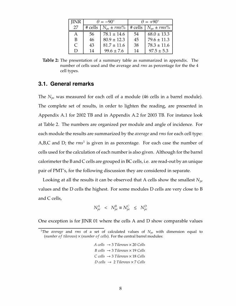
Table 2: The presentation of a summary table as summarized in appendix. Thenumber of cells used and the average and rms as percentage for the the 4cell types.

3.1. General remarks

The Npe was measured for each cell of a module (46 cells in a barrel module).

The complete set of results, in order to lighten the reading, are presented in

Appendix A.1 for 2002 TB and in Appendix A.2 for 2003 TB. For instance look

at Table 2. The numbers are organized per module and angle of incidence. For

each module the results are summarized by the average and rms for each cell type:

A,B,C and D; the rms1 is given in as percentage. For each case the number of

cells used for the calculation of each number is also given. Although for the barrel

calorimeter the B and C cells are grouped in BC cells, i.e. are read-out by an unique

pair of PMT’s, for the following discussion they are considered in separate.

Looking at all the results it can be observed that A cells show the smallest Npe

values and the D cells the highest. For some modules D cells are very close to B

and C cells,

NApe < NB

pe ≡ NCpe . ND

pe

One exception is for JINR 01 where the cells A and D show comparable values

1The average and rms of a set of calculated values of Npe with dimension equal to(number o f tilerows) × (number o f cells). For the central barrel modules:

A cells → 3 Tilerows × 20 CellsB cells → 3 Tilerows × 19 CellsC cells → 3 Tilerows × 18 CellsD cells → 2 Tilerows × 7 Cells

8

Npe(npe/GeV)JINR 01 JINR 13

Cell −90◦ 90◦ −90◦ 90◦

A 77.0±7.7 73.2±8.0 72.5±13.3 63.1±14.3B 81.3±6.7 81.0±8.1 79.5±13.7 80.1±17.3C 82.5±8.6 82.1±6.4 79.7±11.6 76.5±14.1D 74.2±6.3 73.3±6.5 84.7± 8.6 81.7± 6.9

Table 3: Npe from the SLC method using µ at −90◦ and +90◦ for Central Barrelmodules JINR 01 and JINR 13

(77 and 74 pe/GeV respectively) but smaller than the ones in B and C cells (81

and 82 pe/GeV respectively). For all modules the B and C cells values are equal

within the calculated errors as required. However this is not a trivial result since

B and C cells have tiles from different producers with different light yields [11].

An optical mask was introduced in order to achieve the light yield uniformity for

these channels being details given later in Section 3.3.1.

In Tab. 3 data from 2002 TB (JINR 01) and 2003 TB (JINR 13) the two test beam

years for θ = −90◦ and for θ = +90◦ are presented. When comparing the results

for the two years it is observed that they are somewhat different. In the 2002 TB

the differences in Npe for data coming from θ = −90◦ and from θ = +90◦ are

of ∼ 4 pe/GeV (∼ 5%) are found for A cells but for B and C cells the differences

tend to be close to ∼ 1 pe/GeV (∼ 1%); the rms varies between 6.3% and 8.6%.

For the 2003 TB, and making the same comparison, a huge difference going from

∼ 10 pe/GeV (12.5%) is found in the calculated Npe for the A cells. For the B and C

cells the two beam geometries present similar values of Npe but the rms increases

by ∼ 3% for θ = +90◦ for the two cells type but 2x higher than in 2002 TB. The D

cells show for the two years a similar performance. These observations are valid

for other/any pair of modules from the two years.

Although some differences should appear, related with precision on the posi-

tioning and energy of the beam, these are expected to be of the same order and

9

Year Module N−90◦pe −N+90◦

pe N−90◦pe /N+90◦

pe

JINR 34 4.77 ± 8.18 1.05 ± 0.092002 JINR 55 0.44 ± 4.62 1.01 ± 0.06

JINR 01 1.53 ± 4.92 1.02 ± 0.07JINR 27 3.20 ± 10.75 1.07 ± 0.18

2003 JINR 63 2.45 ± 13.08 1.05 ± 0.20JINR 13 3.10 ± 12.43 1.09 ± 0.22

Table 4: The mean and rms for N−90◦pe −N+90◦

pe and N−90◦pe

N+90◦pe

type for the two test beam periods. Nevertheless during the 2003 TB the Npe is

extremely dependent on the orientation of the impinging beam, decreasing this

effect as the cell size increases (A→ D).

3.2. Read-out asymmetries

The muons coming from −90◦ or +90◦ have shown some differences that should

be looked in more detail. In particular it was mentioned in Section 3.1 a clear

difference for the A cells in the 2003 TB period. In the following and first the Npe

are compared cell per cell for each module and test beam period. After that, a

comparison of the charge measured with each read-out PMTs of a cell is made.

3.2.1. Npe difference between θ = −90◦ and θ = +90◦

In Fig. 3 distributions comparing the Npe for the two beam geometries are pre-

sented. The results for each test beam year are combined and the difference

N−90◦pe − N+90◦

pe and ratio N−90◦pe

N+90◦pe

are plotted. These quantities measure the repro-

ducibility of the Npe measurement using the TileCal test beam setup for the two

beam geometries. In Tab. 4 the same quantities are summarized per module using

the mean from the fit and σ of the distributions similar to those presented in Fig. 3.

The discussion will be divided in two parts: first the mean values are compared

10

0

5

10

15

20

25

30

35

0.5 0.6 0.7 0.8 0.9 1 1.1 1.2 1.3 1.4 1.5Npe-90/Npe+90

entri

es

(a) N−90◦pe /N+90◦

pe in 2002 TB

0

5

10

15

20

25

30

-40 -30 -20 -10 0 10 20 30 40Npe-90-Npe+90

entri

es(b) N−90◦

pe −N+90◦pe in 2002 TB

0

2

4

6

8

10

12

14

16

0.5 0.6 0.7 0.8 0.9 1 1.1 1.2 1.3 1.4 1.5Npe-90/Npe+90

entri

es

(c) N−90◦pe /N+90◦

pe in 2003 TB

02468

1012141618

-40 -30 -20 -10 0 10 20 30 40Npe-90-Npe+90

entri

es

(d) N−90◦pe −N+90◦

pe in 2003 TB

Figure 3: The Npe for −90◦ and +90◦ in 2002 TB and 2003 TB. For each year theresults from the different modules are combined in a unique histogram.The difference N−90◦

pe −N+90◦pe and the ratio N−90◦

pe /N+90◦pe are presented.

11

and afterwords a comparison is made over the rms. It is seen that for modules

JINR 55 and JINR 01 (2002 TB) present good reproducibility for the two µ beam

geometries as expressed either by the mean values of N−90◦pe − N+90◦

pe or N−90◦pe

N+90◦pe

. For

JINR 34 and (2002 TB) the reproducibility is poorer and is similar to 2003 TB

results. When comparing the rms for the two years it is seen that the values are

consistently higher for the 2003 TB. For the 2002 TB the worse value of rms is for

the module JINR 34 which follows the larger difference found in the mean value

of the two quantities in discussion. Before drawing out some conclusion a look

over the cells readout asymmetries is presented, comparing the charge signal of

the pair of PMT’s of a cell.

3.2.2. UP to DOWN charge asymmetry

To exemplify the asymmetries found for each cell of a module during the 2002 TB

and the 2003 TB, two modules are used. For 2002 TB the barrel module JINR 01

and for the 2003 TB the barrel module JINR 13. The results for the two TB years

are compared and for each year the θ = −90◦ scan is compared with the θ = +90◦

scan. To characterize these asymmetries the quantity

u − du + d =

Q(u) −Q(d)Q(u) +Q(d)

is used, that is calculated for each cell of a module.

In Tab. 5 the u−du+d is summarized for the two barrel modules JINR 01 and JINR 13.

For each cell type the mean value and corresponding rms of this quantity are

presented. The 2002 TB module JINR 01 has a mean value and the corresponding

rms always below 3% and independent on the ’beam direction’2 of the impinging

beam. This is not observed for the 2003 TB and in particular for the module

JINR 13. First u−du+d is sensitive to the ’beam direction’ being the asymmetries bigger

2This is only used to illustrate the problem: the beam is static and is the orientation is given bythe position of the table supporting the modules

12

u−du+d JINR 01 JINR 13

Cell θ = −90◦ θ = +90◦ θ = −90◦ θ = +90◦

A 1.58±1.77 2.76±1.99 2.36±3.61 6.30±8.07

B 2.07±1.54 2.83±1.61 1.17±3.43 3.69±6.44

C 2.09±1.51 2.43±1.73 0.28±3.28 1.20±4.68

D 1.40±1.55 1.57±2.19 -0.45±2.51 -0.53±2.71

Table 5: Readout asymmetries (u-d/u+d) for the CB modules JINR 01 (2002 TB) andJINR 13 (2003 TB)

for the θ = +90◦. This effect shows also a decreasing tendency as the cell size

increases (A → D). The asymmetry is translated by higher values of the average

and the rms, although the mean value could induce to mis-interpretations due to

the modules geometrical symmetry. To illustrate all these comments the results

for the A cells are plotted in Fig. 4(a) for JINR 01 (2002 TB) and in Fig. 4(b) for

JINR 13 (2003 TB) for each tilerow scan and for each cell. An hypothesis for these

slope and this dependence with the ”beam direction” is related with the table

supporting the modules. During the 2003 TB it was observed that the table could

tilt. The resulting effect of this tilt in the muon data are the read-out asymmetries

of the type described above.

3.2.3. Wrap-up

Can these differences produce a measurable effect in the number of photoelec-

trons? The observed differences between the two years when comparing the

results coming from the two impinging beam geometries (N−90◦pe − N+90◦

pe or the

N−90◦pe /N+90◦

pe ) and the cell readout asymmetries (u-d/u+d) show the same ten-

dency: increasing one when the other increases. However it is not clear how

this influences the Npe although the A cells (smaller width in Y) present a consis-

tent difference during the 2003 TB.

The main objective of the present analysis is to obtain the value(s) of light yield

13

-0.2

-0.15

-0.1

-0.05

0

0.05

0.1

0.15

0.2A1

0 A9 A8 A7 A6 A5 A4 A3 A2 A1 A-1

A-2

A-3

A-4

A-5

A-6

A-7

A-8

A-9

A-10

cell

Θ = -90o

(u-d

)/(u+

d)

-0.2

-0.15

-0.1

-0.05

0

0.05

0.1

0.15

0.2

A10 A9 A8 A7 A6 A5 A4 A3 A2 A1 A-1

A-2

A-3

A-4

A-5

A-6

A-7

A-8

A-9

A-10

cell

Θ = +90o

(u-d

)/(u+

d)

(a) u-d/u+d for JINR 01 in 2002 TB

-0.2

-0.15

-0.1

-0.05

0

0.05

0.1

0.15

0.2

A10 A9 A8 A7 A6 A5 A4 A3 A2 A1 A-1

A-2

A-3

A-4

A-5

A-6

A-7

A-8

A-9

A-10

cell

Θ = -90o

(u-d

)/(u+

d)

-0.2

-0.15

-0.1

-0.05

0

0.05

0.1

0.15

0.2

A10 A9 A8 A7 A6 A5 A4 A3 A2 A1 A-1

A-2

A-3

A-4

A-5

A-6

A-7

A-8

A-9

A-10

cell

Θ = +90o

(u-d

)/(u+

d)

(b) u-d/u+d for JINR 13 in 2003 TB

Figure 4: The u−du+d ratios Vs. Cell number for A cells from CB modules JINR 01

(2002 TB) and JINR 13 (2003 TB). Where the ∗ is for Tilerow 1 � for Tilerow2 and � for Tilerow 3.

14

Tile SizeModule A B C D

1-3 4-6 7-9 10-11JINR 01 PSM #1 PSM #1 PSM #1 PSM #1JINR 12 PSM #1 PSM #1 PSM #1 PSM #1JINR 13 PSM #1 PSM #1 PSM #1 PSM #1JINR 18 PSM #2 PSM #3 BASF #3(M) BASF #3JINR 27 PSM #2 PSM #3 BASF #3(M) BASF #3JINR 34 PSM #2 BASF #4A BASF #4A BASF #4AJINR 55 PSM #2 BASF #4B BASF #4B BASF #4BJINR 63 PSM #2 BASF #4B BASF #4B BASF #4B

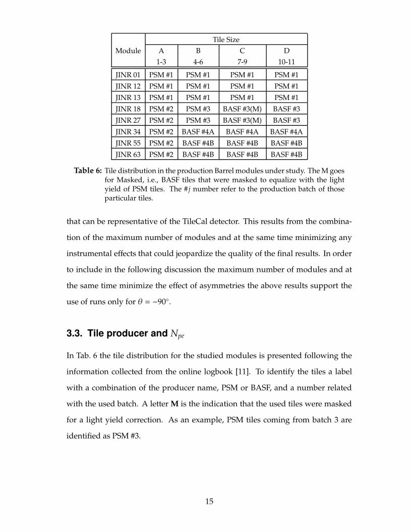
Table 6: Tile distribution in the production Barrel modules under study. The M goesfor Masked, i.e., BASF tiles that were masked to equalize with the lightyield of PSM tiles. The # j number refer to the production batch of thoseparticular tiles.

that can be representative of the TileCal detector. This results from the combina-

tion of the maximum number of modules and at the same time minimizing any

instrumental effects that could jeopardize the quality of the final results. In order

to include in the following discussion the maximum number of modules and at

the same time minimize the effect of asymmetries the above results support the

use of runs only for θ = −90◦.

3.3. Tile producer and Npe

In Tab. 6 the tile distribution for the studied modules is presented following the

information collected from the online logbook [11]. To identify the tiles a label

with a combination of the producer name, PSM or BASF, and a number related

with the used batch. A letter M is the indication that the used tiles were masked

for a light yield correction. As an example, PSM tiles coming from batch 3 are

identified as PSM #3.

15

3.3.1. Masking

To improve uniformity within cells where BASF and PSM tiles are mixed, the

BASF tiles read-out edges were masked. This procedure is illustrated in Fig. 5

where an upper section and a bottom section of the readout edge are painted in

white. It was necessary to use this extra masking in modules JINR 18 and JINR 27.

(a) Painting the tiles edges (b) The resulting masked tiles

Figure 5: The tile edge masking used to reduce the light yield from the tiles producedby BASF. Upper and lower white bands cover a portion of the readout edgeof BASF tiles as a compensation to the higher light yield.

For these modules, A and B cells are PSM and C and D cells are BASF but the tiles

included in the C cells are masked. If the obtained Npe are compared it is verified

that B and C cells match very well,

NPSMpe (B) ≡ NMaskedBASF

pe (C) < NBASFpe (D)

and the D cells have an higher Npe.

16

3.3.2. Comparison with the estimated value of 75 pe/GeV

The number of photoelectrons can be estimated using the energy scale α =

1.2 pC/GeV defined for electrons impinging at θ = 90◦modules of the calorimeter3

and the gain defined to be in use in TileCal PMT’s, G = 105. Since the charge at

the PMT anode can be expressed as,

Q = qe × npe × G

the number of photoelectrons per GeV can be estimated as

Npe =α

qe × G = 75 pe/GeV (3)

This is the number obtained for electrons. For muons the number should be

multiplied by the µ/e factor resulting a value of 82 pe/GeV. This prediction is close

to the number obtained for PSM tiles.

3.3.3. Comparing tile production batches

As shown the Npe is different for the two tile producers. To study this difference

in more detail and to investigate the differences in tiles coming from the same

producer, the results summarized in Tab. A.1 and Tab. A.2 are rearranged by

producer and also by production batch in Tab. 7. Once more the used data comes

only from beams at -90◦.

Tab. 7 has the Npe values obtained for the central barrel module. The last

two columns are the average and rms per batch and the average and rms per tile

producer – PSM and BASF – respectively. The used rms is calculated using only

the Npe entries in this table, neglecting the rms calculated for each cell type (as

presented in Tab. A.1 and Tab. A.2). It is verified that tiles from PSM production

3Recall that this is for the energy reconstructed with the Flat Filter method

17

PS Batch JINR Npe(npe/GeV) (N◦measurements)

Type # A B C D NBATCHpe NPolystyrene

pe

P1 01 77.0 (54) 81.3 (46) 82.5 (45) 74.2 (12)

13 72.5 (53) 79.5 (50) 79.7 (42) 84.7 (14) 78.9 ±4.134 83.6 (51) – – –

PSM P2 55 82.2 (48) – – – 81.0 ±2.4 79.8 ±3.427 78.1 (56) – – –63 79.9 (51) – – –

P3 27 – 80.9 (46) 81.7 (43) – 81.3 ±0.6B3 27 – – – 99.6 (14) 99.6**

BASF B4A 34 – 101.9 (45) 100.7 (42) 104.5 (14) 102.7±1.6 100.6±2.1B4B 55 – 100.6 (48) 100.3 (48) 98.9 (14)

63 – 84.8* (38) 88.7* (35) 97.0 (10) 99.3 ±1.5

Table 7: The Npe in each module per cell type and for each scintillating tile producerbatch. The used numbers come from the SLC method for −90◦. The pre-sented error is the absolute rms of the numbers in this table. (*) Smallernumber due to instrumental test during optics assembly (**) Only one datapoint for batch 3 of BASF and so no rms.

and BASF production show a difference of ∼20 pe/GeV. Typical values of ∼80

pe/GeV for PSM tiles and ∼100 pe/GeV for BASF tiles are found. In Fig. 6 the

plotted values are the averages coming from Tab. 7.

Concluding, the results are insensitive to the batch but a clear difference is

observed between producers as mentioned before. For this reason the results

are combined maintaining the distinction of tile producer and cell type in Tab. 8.

A scaling factor comparing the light yield of tiles coming from BASF and tiles

coming from PSM of

BASF/PSM ' 1.25

is obtained in TileCal for the central barrel modules.

3.3.4. Npe vs. Tiles QC

A quantitative comparison can be done between the scintillating tiles light yield

data obtained during the quality control [11] and the Npe results from beam tests.

18

70

75

80

85

90

95

100

105

110

Tile Production

pe/G

eV

P1 P2 P3 B3 B4A B4B

Figure 6: Npe for 3 batches of PSM (P) and BASF (B) tiles. The values are the averagesand rms from results presented in Tab. 7

Cell type PSM BASFA 78.8 ± 0.5 –B 80.5 ± 0.8 96.4 ± 1.0C 81.3 ± 0.9 97.2 ± 0.9D 79.8 ± 1.6 100.3 ± 1.2

Table 8: The number of photoelectrons per GeV for 90◦ muons, in Tilecal barrelmodules. The average value for each cell type and the respective statisticalerrors – the rms% is divided by the root square of number of measurements– are given separately for PSM and BASF scintillators.

19

2.05

2.1

2.15

2.2

2.25

2.3

2.35

2.4

2.45

2.5

70 75 80 85 90 95 100 105pe/GeV

I 0 /I 1

(a) Io/I1 vs. Npe

110

115

120

125

130

75 80 85 90 95 100 105pe/GeV

I 0

(b) Io vs. Npe

Figure 7: The number of photoelectrons Npe as function of Io/I1 and Io the twoscintillating tiles QC parameters.

From the tiles measurements two quantities are used: Io the light yield and Io/I1

sensitive to the attenuation length. These two quantities are now plotted against

Npe in Fig. 7. From these two plots a correlation is found between the Io and the

Npe as expected but a clear distinction and correlation is only found between tile

producers. Within each producer the fluctuations blur any possible correlation

that could be found between batches of the same producer. These plots confirm

that the higher light yields as measured during the tiles QC corresponds to the

highest number of photoelectrons. For the Io/I1 no correlation is found with the

Npe meaning that the attenuation length is the same for the two producers.

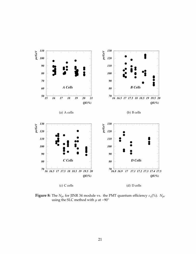
3.4. Quantum efficiency

The correlation between the photomultiplier quantum efficiency εq and the Npe is

now analyzed. In Fig. 8 are shown correlation plots for JINR 34 cells A, B, C and

D. For this module the A cells have tiles made of PSM polystyrene and B, C and

D cells have tiles made of BASF polystyrene. The quantum efficiency for each

20

50

60

70

80

90

100

110

15 16 17 18 19 20 21QE(%)

pe/G

eV

A Cells

(a) A cells

70

80

90

100

110

120

130

16 16.5 17 17.5 18 18.5 19 19.5 20QE(%)

pe/G

eV

B Cells

(b) B cells

70

80

90

100

110

120

130

16 16.5 17 17.5 18 18.5 19 19.5 20QE(%)

pe/G

eV

C Cells

(c) C cells

70

80

90

100

110

120

130

16.8 16.9 17 17.1 17.2 17.3 17.4 17.5QE(%)

pe/G

eV

D Cells

(d) D cells

Figure 8: The Npe for JINR 34 module vs. the PMT quantum efficiency εq(%). Npeusing the SLC method with µ at −90◦

21

PMT was measured during the PMT acceptance quality control. Since the Npe was

calculated per cell for each cell the average of the εq of the two read-out PMTs is

used; which is reasonable since differences between PMTs εq are of the order of 1%

within a cell. From these plots it is not found a clear correlation between the two

quantities but this could be hidden by the huge fluctuations, of the order of 10%,

in the calculated number of photoelectrons when compared with the quantum

efficiency fluctuations of the order of 3%. Even for very small fluctuations on the

εq as of the order of 0.5%, fluctuations on Npe of the order of 10% are observed.

3.5. Npe and Energy resolution

As was expressed during the motivations to this work the Npe contributes to the

energy resolution of TileCal. This results from the definition of Npe since

(

σ

E

)

photostatistics=

1√npe

=1

√

Npe · E=

1/√

Npe√

E

resulting that the energy resolution parameterization can be extended by explicitly

presenting the photostatistics term a2 that is contained in the 1/√

E term, i.e.,

σ

E =a√

E⊕

bE ⊕ c = a1√

E⊕

a2√E⊕

bE ⊕ c (4)

with a2 = 1/√

Npe and E in GeV.

The Npe measurements presented in the previous sections show a strong corre-

lation between Npe and tile producer, but not on their radial position. In Tab. 9

it is shown how this differences influence the energy resolution of the TileCal

detector. It is assumed that the design 50%/√

E term is defined considering the 20

pe/GeV required for the TileCal [1] so that a1 of Eq. 4 is obtained. The new 1/√

E

is calculated using this fixed value of a1 and the Npe measured and presented in

the second column of this table. This is done for two scenarios: considering a

22

Quadratic sum Linear sumSource Npe a2 = 1/

√

Npe a1 a a1 a(pe/GeV) (%) (%) (%) (%) (%)

TDR Minimum 20.0 22.36 44.72 50.00 27.64 50.00

PSM 79.8 11.19 46.10 38.83BASF 100.6 9.97 45.82 37.61

Table 9: Npe and Energy Resolution. The TDR light yield minimum 20 pe/GeV isused with adesign = 50% to determine a1. This value is fixed and com-bined with the photostatistics term to measure the contribution of the Npemeasurements in the energy resolution statistical term.

quadratic sum (a1 and a2 are two independent terms) or a linear sum (some dependence

exists between the two terms) of the two 1/√

E terms as presented in Eq. 4.

The weight of the photostatistics term a2 strongly depends on the parameter-

ization used for the statistical term a, 3% considering the quadratic sum of the

two terms a1 and a2 but aproximately 30% for a linear sum. The current light

yield results improve the statistical term of the energy resolution from 3.9% to

4.2% (quadratic sum) and from 12.2% to 13.4% (linear sum). Comparing the sen-

sibility of cells with PSM and BASF tiles it is obtained a minimum difference of

0.3% (quadratic sum) and a maximum of 1.22% (linear sum) meaning that the

light yield difference of TileCal cells represents a very small effect on the energy

resolution statistical term.

3.6. Signal to noise ratio

Since the TileCal can be used as a muon trigger in ATLAS a clear distinction be-

tween the muon events and the electronic noise events is required. Measurements

using prototypes have shown that the width of the muons response was sensi-

tive to the variation of the Npe [1]. For a variation of the Npe from 20 pe/GeV to

48 pe/GeV a variation is observed in the width of the charge distribution. Above

48 pe/GeV no visible change is observed.

23

The S/N is calculated for θ = 90◦ and η = 0.45 being two definitions used. One

as found in [13]:( SN

)

1= 2 ×

Qµu+d −QPedu+d

σµ

Gauss + σPed

where,

Qiu+d the charge distribution most probable value;

σµ

Gauss the σ of the gaussian component of µ’s charge distribution

σPed the pedestal width.

The second one simply takes the ratio of the Qiu+d of the muons charge distribution

and the noise width:( SN

)

2=

Qµu+dσPed

as was used in [14]. The number index 1 or 2 is used for reference.

The S/N separation is depicted in Fig. 9 for cells A5, BC5 and D2 and the

corresponding tower where all three cells are included. As the signal is the sum

of the individual charge in different PMTs, the noise has been treated in a similar

way. From the histograms it is clear that the signal is well separated from the

noise, although a small overlap between signal and noise is observed for the A

and D cells. In Tab. 10 the used numbers and the calculated S/N for the different

cases are presented. The Qµu+d ≡MOP for the present calculus.

From the calculated values it is observed that when the shift of the pedestal

from zero is not considered, as in the(

SN

)

2equation, the values are consistently

higher. BC cells present the biggest value, an intermediated value is obtained for

D cells and the smallest for the A cells, in agreement with the number of tiles and

tiles sizes in each sampling. The(

SN

)

2for the all tower is approximately 20, which

is half of what was measured during 1996 for the prototypes [14]. An important

aspect is that σPed is 2x larger in the used data (Flat Filter), which simply reduces

24

0

25

50

75

100

125

150

175

200

-0.4-0.2 0 0.2 0.4 0.6 0.8 1 1.2 1.4Q(pC)

Even

ts

(a) Cell A5

0

25

50

75

100

125

150

175

200

-0.5 0 0.5 1 1.5 2 2.5 3 3.5 4Q(pC)

Even

ts

(b) Cell BC5

0

25

50

75

100

125

150

175

200

-0.5-0.25 0 0.250.50.75 1 1.251.51.75 2Q(pC)

Even

ts

(c) Cell D2

0

50

100

150

200

250

-1 0 1 2 3 4 5 6 7 8 9Q(pC)

Even

ts

(d) Tower η = 0.45

Figure 9: Signal noise separation for 180 GeV muons crossing a Central Barrel TileCalmodule for a projective trajectory of η = 0.45 (Flat Filter event reconstruc-tion method)

25

PMT # Qµu+d σµ

Gauss QPedu+d σPed (

SN

)

1

(

SN

)

2Up/Down (pC) (pC) (pC) (pC)A cell 20/21 0.429 0.018 0.136 0.071 3.97 6.04

BC cell 22/23 1.262 0.022 0.242 0.075 7.83 16.83D cell 26/27 0.560 0.019 0.142 0.067 5.18 8.36Tower ALL 6 2.418 0.06 0.385 0.124 9.27 19.51996 4 PMTs 2.66 – – 0.068 – 39.0

Table 10: Signal to noise ratio, from the Flat Filter Method, for muons crossing thecalorimeter for a projective trajectory of η = 0.45. Data from July 2002using Barrel Module JINR 55. The 1996 are results for the prototypesusing projective 150 GeV muons [14]. In energy units and since we have1.2 pC/Gev, 0.136 pC is 113 MeV and so forth.

by half the calculated value of(

SN

)

2. Regarding this comparisons with the 1996

results it should be remarked that:

1. The modules had different radial lengths being bigger in 1996;

2. The used PMT’s used in 1996 were different;

3. In 1996 only the two most energetic cells (4 PMTs) were considered but now

the tower uses 6 PMT’s;

4. Conclusions

In this note the number of photoelectrons for TileCal was measured for 6 Central

Barrel production modules. Sets of runs of 180 GeV muons entering the detector

at θ = ±90◦ (η = ±∞) were used allowing a study per cell to be made. This

resulted in 176 measurements

20[ACells] × 3 + 18[BCells] × 3 + 16[CCells] × 3 + 7[DCells]

for each module and beam geometry. The differences found on the cells are due

to the scintillating tiles producer; in fact a difference of ∼ 25% was found between

26

the BASF tiles (∼ 100 pe/GeV) and PSM tiles (∼ 80 pe/GeV) being this in agreement

with the light yield differences measured in laboratory for the different batches

of tiles coming from these two producers. The number found for the PSM tiles

shows to be in very good agreement with the prediction of 82 pe/GeV based in

well established parameters of the detector. The results were further compared

with the quantum efficiency of the TileCal photomultipliers and there was no

evidence of a relation between quantum efficiency and light yield. The influence

of the number of photoelectrons on fundamental performance characteristics of

the detector as the signal to noise ratio and energy resolution was also looked at.

It was shown that the difference of light yields in TileCal cells imply a variation

in the statistical term of the energy resolution less than 1.2%. The signal to

noise ratio gave values of the order of 20 for the energy reconstructed with the

Flat Filter method; but notice that it is well known the lack of precision of this

reconstruction method for pedestal measurements giving signals 2x larger than

on TileCal prototypes and presently seen on TileCal production modules when

using a different event reconstruction method – Fit method. To conclude, (1) the

TileCal detector shows a light yield level compatible with the design requirements

for resolution and signal to noise separation and (2) the Slice Method has been

found to be an efficient method to obtain a light yield in agreement with simple

characteristics of the detector as the PMT gain and energy scale for electrons.

5. Acknowledgment

The work described in this document was supported by a grant within the project

’Calorımetria para ATLAS/LHC’ POCTI/FNU/49527/2002.

27

References

[1] TileCal Collaboration ’Tile Calorimeter Technical Design Report’

CERN/LHCC 96-42

[2] A. Bernstein et al. Beam tests of the ZEUS barrel calorimeter. Nucl. Inst. and

Meth. in Phys.,A336:23-52, 1993.

[3] J. Proudfoot, R. Stanek ’An Optical Model for the Prototype Module Per-

formance from Bench Measurements of Components and the Test Module

Response to Muons’ ATL-TILECAL-95-066 Geneva : CERN, 25 Oct 1995

[4] J. Proudfoot ’Light yield in the extended barrel prototype modules from

electrons at 90 degrees’ ATL-TILECAL-97-133 Geneva : CERN, 28 Nov 1997

[5] S. Nemecek, T. Davidek, R. Leitner ’Light Yield Measurement of the 1998 Tile

Barrel Module0 using muon beams’ ATL-TILECAL-99-003 Geneva : CERN,1

Feb 1999

[6] V. Castillo, F. Fassi ’Light yield and uniformity of the TileCal Barrel Module

0 prototype’ ATL-TILECAL-2000-001 Geneva : CERN, 13 Jan 2000

[7] Z. Azaltouji et al. Response of the ATLAS Tile calorimeter prototype to

muons. Nucl. Inst. and Meth. in Phys, A388:64-78, 1997.

[8] S. Tokar ’PMT Excess Factor’ TileCal Week/Tools and MC Session, 15 Oct

2001

[9] V. Garde ’ Controle et etalonnage par lumiere laser et par faisceaux de muons

du calorimetre hadronique a tuiles scintillantes d’ATLAS ’ Universit Blaise

Pascal, 2003

[10] T. Davidek, R. Leitner ’Parametrization of the Muon Response in the Tile

Calorimeter’ ATL-TILECAL-97-114 Geneva : CERN, 10 Apr 1997

28

[11] http://altair.ihep.su/ konstant/qc/scintillator.html

[12] http://tilecal.in2p3.fr/pmt/accueil/accueil.php

[13] A. Camard, F. Hubard , B. Laforge ; P. Shemling ’Study of the EM barrel with

muons’ ATL-LARG-2001-017 Geneva : CERN, 2001

[14] S. Alkhamadaliev et al. Results from a new combined test of an electromag-

netic liquid argon calorimeter with a hadronic scintillating-tile calorimeter.

Nucl. Inst. and Meth. in Phys., A449:461–477, 2000.

29

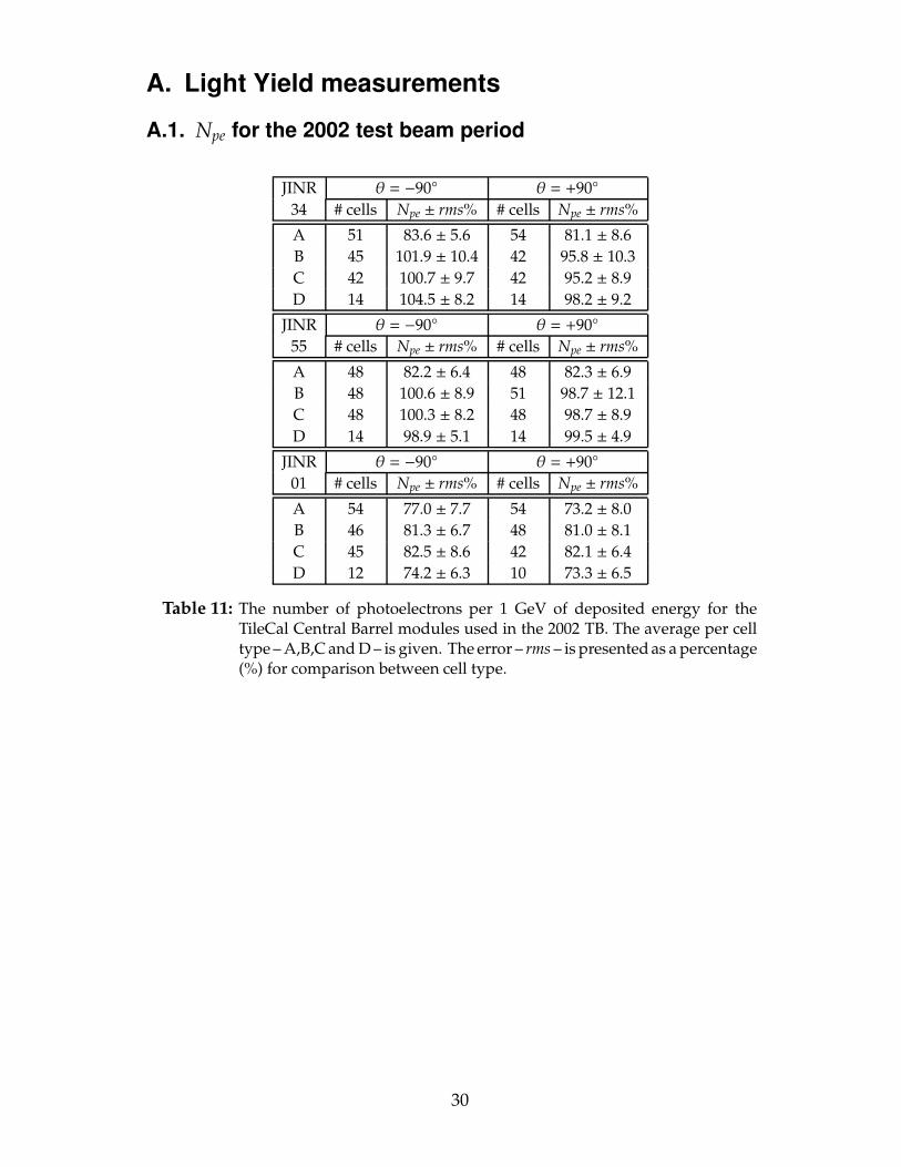
A. Light Yield measurementsA.1. Npe for the 2002 test beam period




Table 11: The number of photoelectrons per 1 GeV of deposited energy for theTileCal Central Barrel modules used in the 2002 TB. The average per celltype – A,B,C and D – is given. The error – rms – is presented as a percentage(%) for comparison between cell type.

30

A.2. Npe for the 2003 test beam period




Table 12: The number of photoelectrons per 1 GeV of deposited energy for theTileCal Central Barrel modules used in the 2003 TB. The average per celltype – A,B,C and D – is given. The error – rms – is presented as a percentage(%) for comparison between cell type.

31

A.3. Settings of PAW and differences on the presented dataIn some steps in the processing of the present analysis the use of means and rmsis needed. Altough the PAW gives these numbers by default it needs some caresince, and also by default, this is a weighted number over the binning

< x >=∑nbin

i=1 ci × ni∑nbin

i=1 ni=

∑nbini=1 ci × ni

N (5)

and not the real average as given by:

< x >=∑N

i=1 xi

N (6)

where,<x > the statistical average of the quantity x we are studing;

nbin the number of bins in the histogram;

ci the value of x that corresponds to the mean point of bin i;

ni the number of entries in bin i;

N the total number of events;

pe/GeV (Slice Method) HSTAT off70 80 90 100 110 120

pe/GeV (Slice Method) HSTAT off70 80 90 100 110 120

pe/G

eV (S

lice

Met

hod)

HST

AT O

n

70

80

90

100

110

Figure 10: Comparing two PAW settings for the retrieving of statistical informationfrom histograms. A linear fit to the points gives y = (0.957 ± 0.007) × x +(2.8 ± 0.7)

This real average (Eq. 6) can be obtained if we set within the PAW the option’OPTION HSTAT’. During the analysis described in this note we have used thedefault settings in PAW and so the undesired average was used. For futurereference the numbers for θ = −90◦ were recalculated setting this option ON anda comparison is presented in Fig. 10.

The plot in Fig. 10 and summary table Tab. 13 show that the differences thatresult from the comparison of both cases is not relevant in terms of light yieldlevel as expected.

32

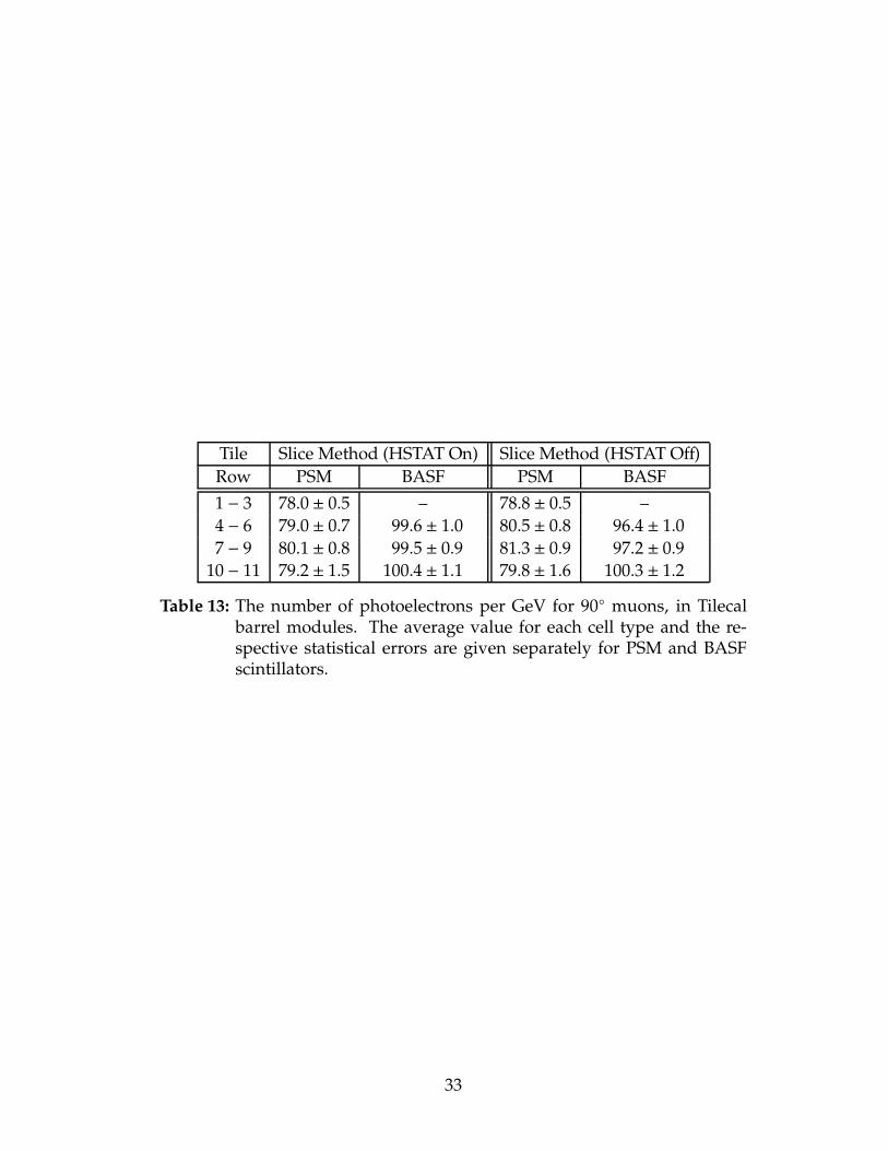
Tile Slice Method (HSTAT On) Slice Method (HSTAT Off)Row PSM BASF PSM BASF1 − 3 78.0 ± 0.5 – 78.8 ± 0.5 –4 − 6 79.0 ± 0.7 99.6 ± 1.0 80.5 ± 0.8 96.4 ± 1.07 − 9 80.1 ± 0.8 99.5 ± 0.9 81.3 ± 0.9 97.2 ± 0.9

10 − 11 79.2 ± 1.5 100.4 ± 1.1 79.8 ± 1.6 100.3 ± 1.2

Table 13: The number of photoelectrons per GeV for 90◦ muons, in Tilecalbarrel modules. The average value for each cell type and the re-spective statistical errors are given separately for PSM and BASFscintillators.

33

light yield studies of the atlas tile calorimeterdavidek/joao.pdflight yield studies of the atlas...

Documents