light scattering characteristics of various aerosol types derived from multiple wavelength lidar...

Light scattering characteristics of various aerosol typesderived from multiple wavelength lidar observations

Yasuhiro Sasano and Edward V. Browell

The present study demonstrates the potential of a multiple wavelength lidar for discriminating betweenseveral aerosol types such as maritime, continental, stratospheric, and desert aerosols on the basis of

wavelength dependence of the aerosol backscatter coefficient. In the analysis of lidar signals, the two-

component lidar equation was solved under the assumption of similarity in the derived profiles of backscattercoefficients for each wavelength, and this made it possible to reduce the uncertainty in the extinction/

backscatter ratio, which is a key parameter in the lidar solution. It is shown that a three-wavelength lidar

system operating at 300,600, and 1064 nm can provide unique information for discriminating between various

aerosol types such as continental, maritime, Saharan dust, stratospheric aerosols in a tropopause fold event,and tropical forest aerosols. Measurement error estimation was also made through numerical simulations.Mie calculations were made using in situ aerosol data and aerosol models to compare with the lidar results.

There was disagreement between the theoretical and empirical results, which in some cases was substantial.

These differences may be partly due to uncertainties in the lidar data analysis and aerosol characteristics andalso due to the conventional assumption of aerosol sphericity for the aerosol Mie calculations.

1. Introduction

The lidar technique, in principle, can measure theatmospheric backscatter coefficient, 1 which is equiva-lent to the integral of the aerosol backscatter crosssection with the aerosol size distribution as the weight-ing function. The aerosol backscatter cross section isuniquely determined according to the physical andchemical properties of the aerosols (their size, shape,and complex refractive index) and the laser wave-length, and the wavelength dependence of the back-scatter coefficient is mainly dependent on the aerosolsize distribution and refractive index. A multiplewavelength lidar can, in principle, be used to measurethe wavelength dependence of the aerosol backscattercoefficients.

Different aerosol types are expected to have differ-ent size distributions and refractive indices, which im-plies that it may be possible to discriminate aerosoltypes according to the wavelength dependence ob-served by a multiple wavelength lidar. Recent theo-

Yasuhiro Sasano is with National Institute for EnvironmentalStudies, Tsukuba, Ibaraki 305, Japan; and E. V. Browell is withNASA Langley Research Center, Hampton, Virginia 23665-5225.

Received 17 March 1988.0003-6935/89/091670-10$02.00/0.0 1989 Optical Society of America.

retical calculations also suggest this possibility. Forexample, Wood2 calculated the backscatter coeffi-cients for maritime and continental aerosol modelsusing the Mie theory and found that the two types ofaerosol can be discriminated by the difference in wave-length dependence of the backscatter coefficients withan appropriate combination of lidar wavelengths.Whitlock et al.3 analyzed Mie calculations for variousaerosol models and showed that the ratio of backscat-ter coefficients for wavelengths of 550 and 1040 nm hasa different value for different aerosol models. Thisindicates the possibility of discriminating betweenaerosol types. Also, Shettle4 has shown the depen-dence of aerosol backscatter on the type of aerosol andvariations in relative humidity. Aerosol extinctioncoefficients have been shown by Shettle and Fenn5 tohave the same kind of wavelength-dependent varia-tion with aerosol type.

This study shows the differences in the wavelengthdependence of aerosol backscatter coefficients derivedfrom atmospheric measurements made by an airbornemultiple wavelength lidar. The airborne observationsdiscussed here were made primarily over the southwestof the United States of America, the tropical Atlantic,and French Guyana. Data were obtained from lidarsignals at 300, 600, and 1064 nm for various types ofaerosol such as continental, maritime, Saharan dust,stratospheric aerosols in a tropopause fold event, andtropical rain forest aerosols. In situ measurements ofaerosol size distributions were made simultaneously

1670 APPLIED OPTICS / Vol. 28, No. 9 / 1 May 1989

with the lidar observations. Mie calculations weremade using the in situ aerosol data compared with thelidar data. The analysis presented in this paper pro-vides a basis for future studies of the discrimination ofaerosol types from multiple wavelength lidar observa-tions.

Fernald's solution for the two-component lidarequation was adopted to analyze the lidar data.6 Inthis solution a boundary condition and an extinction/backscatter ratio are needed. To provide a boundarycondition, the so-called matching method was utilizedwith the assumption of an aerosol-free layer. Theextinction/backscatter ratio is, in general, an unknownparameter; however, it can be estimated by assumingthe similarity between the solution profiles for differ-ent wavelengths and taking into account that the back-scatter coefficient profile for a longer wavelength hasless sensitivity to the extinction/backscatter ratio thanthose for a shorter wavelength.

:1j(R) = - 2(R) +

The basic idea for the present analysis has beendescribed by Sasano and Browell.7 Recently Potter8

proposed an alternate technique that seeks simulta-neously for the two extinction/backscatter ratios at thetwo lidar wavelengths and the total transmittance(which is equivalent to assigning the boundary condi-tions) with the same criterion of maximizing the simi-larity in the solution profiles. While this approach haspotential, it has yet to be verified with experimentaldata.

In the following section, the methods for analyzingthe lidar data and for estimating the power-law expo-nent for the wavelength dependence of the backscattercoefficient are described, and an outline of the experi-ments and the results of the empirical aerosol wave-length-dependence analysis are presented. Themethod of Mie calculation and the optical propertiesestimated from the in situ data are discussed in Sec.III. In Sec. IV, the model simulation is describedwhich gives the error estimation in the lidar data anal-ysis, and the study results are discussed in Sec. V withrespect to using multiple wavelength lidar data in theremote discrimination of aerosol types.

11. Analysis of Lidar Data

A. Analysis Technique

The received signal from a lidar system can be ex-pressed generally by the lidar equation':

P(R) = C 1(R) + 32(R)]T2(R)/R2, (1)

T(R) = exp{-f [al(r) + 2(r) + a3(r)]dr} (2)

where P(R) is the received signal for range R; C is thecalibration constant including the laser output power;

fl and 2 are the aerosol and air molecular volumebackscatter coefficients, respectively; al and a2 are theaerosol and air molecular volume extinction coeffi-cients (not including absorption by gases at the lidarwavelength), respectively; a3 is the volume absorptioncoefficient for absorbing gases not included in a2; andT is the atmospheric transmittance.

The extinction/backscatter ratios are defined as fol-lows:

S1 = al/f,1 for aerosols (subscript 1),

S2 = a 2/02 for air molecules (subscript 2),

(3)

(4)

where S2 is a constant for air molecules, and at aspecific wavelength S is a variable dependent on thecharacteristics of aerosols. In our analysis we assumethat S1 is independent of range.

According to Fernald,6 the solution for the lidarequation can be obtained from Eqs. (1)-(4), that is,

X(R) exp 2(S/S 2 ) fA a2 (r)dr1

(R,) + S2 (RR) SJ X(r) exp [-2(SlIS 2 ) J C2(r)dr]dr

, (5)

where

X(R) = P(R)R2 exp [2 J la2(r) + a3(r)ldr]I (6)

which is the lidar signal corrected for the attenuationdue to range, air molecules, and gas absorption. AsFernald,6 Klett,9 and Sasano and Nakane10 show, thesolution for the lidar signal depends on the extinction/backscatter ratio and the boundary condition f 1(Ro),where Ro is the range where the boundary condition isapplied. When R > R, the solution is obtained byforward integration, and when R < R, backward inte-gration is used. The forward integration, in general,gives a more unstable solution that is particularly sen-sitive to the assumed extinction/backscatter ratio andthe boundary condition. For a relatively clean atmo-sphere, however, the backscatter coefficient derivedfrom Eq. (5) is less sensitive to the extinction/back-scatter ratio S.6

The following information is required to solve thelidar equation from the observed lidar signal: theextinction coefficient a2 and the backscatter coeffi-cient 2 for air molecules, the absorption coefficient 3for additional absorbing gases, a boundary condition01(Ro), and the extinction/backscatter ratio S1.Among the above parameters, a2 and 032 can be ob-tained by appropriate meteorological measurementsor a model atmosphere. In this study, the air densityprofiles are assumed to be given by exponential func-tions with scale heights which give good approxima-tions to the tropical atmospheric model by McClat-chey et al.11 for the observations in the tropical regionsand to the U.S. Standard Atmosphere'2 for the mid-latitude observations. The present study analyzes thelidar data for wavelengths of 300, 600 and 1064 nm and

1 May 1989 / Vol. 28, No. 9 / APPLIED OPTICS 1671

only the absorption due to ozone at 300 nm is takeninto consideration. The ozone absorption coefficientswere calculated from in situ ozone measurements ofsimultaneous DIAL ozone measurements.' 3 '15

The boundary condition is an unknown; however, itmust be specified. We adopted the so-called matchingmethod which is often used to analyze lidar data forstratospheric aerosols.'6 The matching method as-sumes an aerosol-free layer at a certain altitude(matching height), and thus the lidar signal from thereis assumed to result only from air molecules. Thematching height is set to the altitude of the minimumvalue for X(R)/1 2(R). The effects on our analysis thatresult from errors in the boundary conditions are ana-lyzed by numerical simulation in Sec. IV.

The extinction/backscatter ratio Si is also an un-known parameter. Although it is highly dependent onthe size distribution and refractive index, it is general-ly expected to take a value between 0.0 and 90.0.17,18Substituting 0.0 for Si means that no corrections aremade for attenuation due to aerosols. The value of90.0 is considered as a reasonable maximum value forS1 . Therefore, putting 0.0 and 90.0 in S1 gives tworeasonable extremes in the solution, which we callmethod 1. The true solution profile is expected to fallbetween those two extreme profiles.

Once the backscatter coefficient profiles are ob-tained at the two lidar wavelengths, a parameter ex-pressing the wavelength dependence is estimated fromthe relation which was derived assuming a power-lawwavelength dependence of the aerosol backscatter co-efficient, that is, 1(X2 ) = 01(XI)M(0/X2 )6. Then

3 =-I/3 1(A)//l(X9)/lnPzl/X9, (7)

where XI and X2 are the wavelengths used.Two profiles are obtained corresponding to SI = 0.0

and S2 = 90.0 for each wavelength, and we denote thebackscatter profiles lB(X,,0.0), 03(X 1 ,9O-O), O(X 2,0-0),and 00(X2,90-0). Then we can estimate the parametersfor the wavelength dependence min(X1,X2) and6max(X1,X 2) from the combinations of f1(X1,0.0) andf3(X 2 ,90.0) and 01(X,,9O.O) and OA(X 2 ,0-0), respectively.Here the t1 and 6 terms are altitude dependent func-tions. Method 1 described here is relatively primitivebut useful in cases with relatively small optical thick-ness.

As described previously, the backscatter coefficientprofile that is obtained in the case of small opticalthickness is relatively insensitive to the extinction/backscatter ratio. Therefore when the lidar signal forthe wavelength of 1064 nm is analyzed by using S, = 0.0and 90.0, backscatter profiles which are more indepen-dent of the extinction/backscatter ratio are obtainedbecause the optical thickness is smaller at 1064 nmthan at 300 and 600 nm.

We assume here that the true profiles of the back-scatter coefficient for the three wavelengths are similarto each other; that is, the profiles are assumed to bedetermined only by the profile of the total numberdensity of aerosols. This implies that the size distri-bution and the refractive index for the aerosols are

invariant across the aerosol layer of interest along thelaser path. Under the above assumptions, we can inferthe extinction/backscatter ratios for the 300- and 600-nm signals which give similar profiles to the 1064-nmprofiles. Here, the profiles for the 1064-nm signal areobtained with SI = 0.0 and 90.0 and are considered asstandards because of weak dependence on the extinc-tion/backscatter ratio. The backscatter coefficientprofiles thus obtained are used to calculate the param-eter . This technique of requiring similarity in thebackscatter coefficient profiles is called method 2.

The actual procedure for method 2 is as follows:First we solve the lidar signal for 1064-nm wavelengthby using Eqs. (5) and (6) with the boundary condition

(Ro) = 0.0 at R = Ro and with the extinction/back-scatter ratio S1 = 0.0 and 90.0. Then as an index ofdegree of similarity, we define the performance func-tion J(Sl)

J(S ) = I ,Rj)_ A IlA^i1i=il 2(Si 02(X0,R)2

where X0 = 1064 nm, X = 300 nm (or 600 nm); SI is theextinction/backscatter ratio to be determined; il and i2are the lower and upper limits for estimating the per-formance function; and A is a proportionality constantthat is determined to minimize J(Sl) for each S1 by aprocedure of the usual least-squares method.

The simplest mapping procedure'9 was adopted todetermine the extinction/backscatter ratios whichwould produce the minimum J(S,). The extinction/backscatter ratios are determined by using the stan-dard profiles obtained with the use of both SI = 0.0 and90.0 from the 1064-nm lidar signal.

B. Results

Table I lists the experiments and types of aerosolthat were studied. Experiments (II), (III), and (IV)were conducted during the NASA Global Tropospher-ic Experiment-Atlantic Boundary Layer Experiment(GTE/ABLE-1) near Barbados in June 1984,2021 andexperiment (V) was conducted over southern Nevadain April 1984.15

Figures 1 (a)-(e) show the lidar signals at 1064 nm formeasurements across layers containing various typesof aerosol. The profiles are presented as the scatteringratios which were calculated with the use of Si = 0.0(solid curve) and 90.0 (dashed curve). The scatteringratio is defined as a ratio of the total atmosphericbackscatter from aerosols and air molecules to thebackscatter from air molecules. The profiles for thecontinental [Fig. 1(a)], the rain forest (Fig. 1(d)], andthe tropopause fold [Fig. 1(e)] aerosols have no distinc-tion between the solid and dashed curves because ofsmall optical thickness. In the figures, the hatchedregions represent the layers which contain the aerosoltypes of interest. The aerosol types were definedbased on the analysis of in situ aerosol data obtained atthe time of the lidar measurements. The wavelengthdependence parameter 6 was derived from the lidarsignals at the altitudes indicated by the triangles.


Table 1. Multiple Wavelength Lidar Experiments

Aerosol Type Case Date Time (GMT) location Aircraft Alt (m ASL)Lat. Long.

Continental (I) 3/23/84 16:54 37.8' N 75.5' W Ground(Upward-looking)

Maritime (11) 6/30/84 14:31 20.5' N 66.8' W 4530

Saharan Dust (Il-a) 6/25/84 4:48 13.1' N 56.5' W 5340(III-b) 6/27/84 18:09 9.2' N 58.2' W 5965

Rain Forest (IV) 6/27/84 15:58 2.3' N 57.0' W 3480

Tropopause Fold (V-a) 4/20/84 22:30 34.7' N 114.7' W 7740(Stratospheric) (V-b) 4/20/84 .22:04 34.0' N 114.6' t 7740

7

Ex

5w0

4

3

2

10SCATTERING RATIO

5

E

-4

ao3

-2I-

J

0

10SCATTERING RATIO

5

E

w

0

I-

-j

4

3

2

100 1

7

E

Uj5

- 4

-J

3

2

100

10SCATTERING RATIO

10SCATTERING RATIO

E

-4

03I-

2-j

1

0 0

00 10SCATTERING RATIO

100

.1 Fig. 1. Scattering ratio profiles calculated100 with S1 = 0.0 (solid) and 90.0 (dashed) for

the lidar signals at a wavelength of 1064 nm.


(b) MARITIME III)

i I . . I I . . .

(d) RAIN FOREST (IV)

1

I . .. I I, . .

61

111

1

CD0

010

U,

AD

_Z -I J I61300, 6001

I J 4

Fig. 2. Diagram of the wavelength dependence parameters derivedwithout attenuation correction (symbols) and by method 1 (boxes).

The ranges of 6 (300,600) and 6 (600,1064) for eachaerosol type are shown in Fig. 2 as a box which indi-cates the ranges of 6min and 6max obtained from method1 using S5 = 0.0 and 90.0. The uncertainty in 6 for thecombination of 300 and 600 nm is too large to discrimi-nate the difference in aerosol types. The effect of theaerosol attenuation correction is large, especially forthe lidar signals at 300 nm, and resulting aerosol dis-crimination using 300 and 600 nm is ambiguous.

The symbols in Fig. 2 indicate the 6 terms obtainedby putting Si = 0.0 for all wavelengths. In that case,no correction was made for the aerosol attenuation atany of the wavelengths.

Figure 3 shows the results of applying method 2.The values were determined with very small ambigu-ity, and this makes it possible to discriminate betweenthe maritime, rain forest, and Saharan aerosols.

The S5 values estimated by applying method 2 arelisted in Table II. The values of 0.0 and 90.0 are shownfor the cases where they were used as standards (at1064 nm) or where method 2 could not produce betterdefined limits.

3

- 2(D

'r-U,

0-1

0'00

-1

-2 -1 0 1 2 3 46(300, 6001

Fig. 3. Diagram of the wavelength dependence parameters derivedby additional application of method 2.

111. Mie Calculations with In Situ Aerosol Data

For the purpose of this analysis, we assume that theaerosols investigated were homogeneous and spheri-cal. The volume backscatter coefficients can then becalculated by the Mie theory when the aerosol sizedistribution, refractive index, and wavelength of lightare given. In situ aerosol measurements were madesimultaneously with most of the lidar measurementsdescribed in the previous section. These aerosol mea-surements were made by a quartz crystal microbalance(QCM) and a forward scattering spectrometer probe(FSSP). The QCM give the aerosol mass distributionas a function of aerosol diameter over nine ranges from0.11 to 40.0 Aim, while the FSSP gives the aerosolnumber density distribution as a function of aerosoldiameter over eight ranges from 0.50 to 4.0,4m. Infor-mation on the in situ aerosol measurements is given inTable III.

According to the Mie theory,22 the volume backscat-ter coefficients fl can be calculated by the followingequation:

Table 11. Ranges of Extinction to Backscatter Ratio Estimated by Method 2

Aerosol Type Case 2= 300 nm 2= 600 nm 2= 1064 nm

S (min) S 1(max) S 1 (max) S 1(min) S1 (min) S1 (max)

Continental (I) 36.2 36.4 [ 0.01 [90.0] [ 0.0] [90.01

aritime (II) 5.1 19.4 [ 0.0] 30.0 [ 0.0] [ 90.0]

Saharan Dust (Ill-a) 55.0 57.3 20.1 61.7 [ 0.0] [ 90.0](Ill-b) 51.1 52.7 15.1 58.0 [ 0.0] [ 90.0]

Rain Forest (IV) 34.5 34.9 42.6 60.0 [ 0.0] [ 90.0]

Tropopause Fold (V-a) [ 0.0] [90.0] [ 0.0] [90.01 [ 0.0] [90.0](Stratospheric) (V-b) 13.9 14.4 [ 0.0] [ 90.0] [ 0.0] [90.0]

Values in [ ] were assumed for the 1064 n signals as the standards and for the signals which could not getbetter defined limits by Hethod 2.


METHOD1}

3

CONTINENTAL TROPOPAUSE FOLD

2 . u X {~~~~~~~STRATOSPHERIC)MARITIME

1 {| * { * F. - RAIN FOREST

SAHARAN DUST

SJ=O.O

0 CONTINENTAL_1 ~~~~~~~~~~A MARITIME

* SAHARAN DUSTA RAIN FORESTV TROP OPAUSE FOLD

METHOD 2 1 = }

TROPOPAUSE FOLD

CONTINENTAL ISTRATOSPHERIC)

E

- RAIN FOREST

MARITIMESAHARAN DUST

k

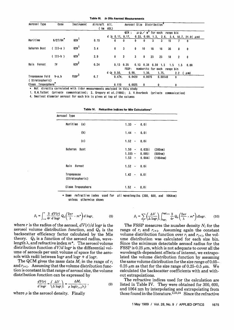
Table 111. In Situ Aerosol Measurements

Aerosol Type Case Instrument Aircraft Alt. Aerosol Size Distribution4(km ASI)

GC : 9g/ me for each range bind 2 0.11, 0.17, 0.33, 0.69, 1.3, 2.6, 5.4, 10.7, 21.0( m)

Maritime 6/27/84* 0CH 0.15 0 0 0 0 3 3 15 7 0

Saharan Dust (III-a) QCM1 3.4 0 3 0 10 18 16 36 8 0

(Ill-b) QCM1 2.9 0 2 3 8 23 23 18 2 0

Rain Forest IV 0CM2 0.24 0.13 0.25 0.13 0.38 0.50 1.5 1.5 1.5 0.88FSSP: number/cc for each range bin

d 0.50, 0.90, 1,30, 1.75, 2.2 ( gm)Tropopause Fold V-a,b FSSP3 6.7 0.474, 0.0420 0.0076 0.00149 0( Stratospheric)Clean Troposphere* 0.110 0.0025 0 0 0* Not directly correlated with lidar measurements analyzed in this study1. R.W.Talbot (private communication); 2. Gregory et al.(1986); 3. V.Overbeck4. Smallest diameter aerosol for each bin is given at top of the columns

(private communication)

Table IV. Refractive Indices for Mie Calculations

Aerosol Type

Maritime (a)

(b)

(c)

Saharan Dust

1.33 - 0.Oi

1.44 - 0.Oi

1.52 - 0.Oi

1.59 - 0.035i1.555 - 0.005i1.53 - 0.004i

Rain Forest

Tropopause(Stratospheric)

Clean Troposphere

(300nm)(600nm)(1 064nm)

1.52 - 0.Oi

1.42 - 0.Oi

1.52 - 0.Oi

* Same refractive index usedunless otherwise shown

__= 4r OgQ *d logr , (8)

where r is the radius of the aerosol, dV(r)/d logr is theaerosol volume distribution function, and Qb is thebackscatter efficiency factor calculated by the Mietheory. Qb is a function of the aerosol radius, wave-length X, and refractive index m*. The aerosol volumedistribution function dV/d logr is the differential vol-ume of aerosols per unit volume of space for the aero-sols with radii between logr and logr + d logr.

The QCM gives the mass data Mi in the range of riand ri+,. Assuming that the volume distribution func-tion is constant in that range of aerosol size, the volumedistribution function can be expressed by

dV(r) A AV AMi (9d logr \\ ogri p og(rj+1/rj)

where p is the aerosol density. Finally

for all wavelengths (300, 600, and 1064nm)

l = ( I AV N o ,:;- 3 Qb (2rr m*) dlogr. (10)

The FSSP measures the number density Ni for therange of ri and ri+j. Assuming again the constantvolume distribution function over ri and ri+,, the vol-ume distribution was calculated for each size bin.Since the minimum detectable aerosol radius for theFSSP is 0.25 Am, which is not adequate to cover all thewavelength-dependent effects of interest, we extrapo-lated the volume distribution function by assumingthe same volume distribution for the size range of 0.05-0.25 m as that for the size range of 0.25-0.5 m. Wecalculated the backscatter coefficients with and with-out extrapolations.

The refractive indices used for the calculation arelisted in Table IV. They were obtained for 300, 600,and 1064 nm by interpolating and extrapolating fromthose found in the literature.2232 4 Since the refractive


index for the rain forest aerosols have not been exam-ined so far, we arbitrarily assumed a value of 1.52-0.Oi,which applies to clear tropospheric aerosols. Al-though the aerosol density p appears in Eq. (10) aftersubstitution from Eq. (9), the wavelength parameter 3is independent of aerosol density.

Figure 4 shows the calculated distributions of (300,600) and 6 (600,1064) for various types of aerosol.A box is used to display the minimum and maximumvalues of 3 for two sets of the Saharan aerosol data.Boxes are also used for the tropopause fold and cleantropospheric aerosol data to show their minimim andmaximum values due to calculation with and withoutextrapolation of the volume distribution function tosmaller radii.

The change in wavelength parameter calculated forthe maritime aerosols using different refractive indicesindicates a potential for determining information onthe composition of marine aerosols, since the refractiveindices and thus the wavelength dependence for back-scatter depend on the refractive index of the compo-nents.

The large negative value of 6 (300,600) for the Saha-ran dust aerosols results from the large imaginary partof the refractive index.

IV. Error Estimation by Numerical Simulation

Since it is difficult to estimate systematic errors inthe analysis of the real lidar data because we do nothave complete information on the distribution andoptical properties of the aerosols of interest, we mustuse results from experiment simulations.

Lidar return signals are simulated for three laserwavelengths with an assumed aerosol distribution andaerosol extinction/backscatter ratio. When analyzingthe lidar signals by methods 1 and 2, errors were inten-tionally given to the boundary conditions to investi-gate the effects of erroneous boundary conditions onthe backscatter coefficients and on the wavelengthdependence parameter , which are the solutions forthe simulated signals.

The model distribution of the aerosols in the atmo-sphere is divided into three layers; one is a clean layerabove a height h 1, another is a transition layer from theclean layer to a turbid aerosol layer below h2; and thethird is the turbid aerosol layer of interest. This aero-sol distribution is expressed by the following equa-tions:

/3(Z)/132(z) = b, for z 2 hi,

= (z-h2) h - h2 + b2 for h > z _ h2,

for z < h2,

where 4000 and 2500 in are assigned to h and h2,respectively. To examine various conditions, b is setto values of 0.0, 0.05, and 0.1 with b2 having values of1.0,5.0 and 20.0. These parameters apply to the 1064-nm wavelength, and those for other wavelengths werespecified using the assumption that Al is proportionalto A-,.

3

-2"4.CD0-10CD

la0

-1

MIE CALC. WITH IIN SITU AEROSOL DATA

CLEAN TROPOSPHERIC

MARITIME El___ TROPOPAUSE FOLD

a Ab (STRATOSPHERIC)

SAHARAN DUST '

zC-Aa ARAIN FOREST

-2l -1 0 2 3 I-2 -1 0 l 2 3 4

6(300, 600)

Fig. 4. Diagram of wavelength dependence parameters calculatedby the Mie theory using in situ aerosol data.

w2

I--J

0 1 2

jP 3*(Z

Fig. 5. Model distribution of aerosol1064 nm.

(lo-6 m- 1sr-l)

backscatter coefficients at

Figure 5 shows the assumed model distributions forthe aerosol backscatter coefficients. The extinction/backscatter ratio Si was assumed to be 50.0 in thesimulation, and the lidar signals, which were calculat-ed for each wavelength from the model profiles, wereanalyzed by using methods 1 and 2. As discussedbefore, it is difficult to prescribe a boundary conditioncorrectly without additional information, and one isforced to use the so-called matching method. In oursimulations, the matching method was also appliedand jl = 0.0 was assigned at the altitude of the match-ing level, which in our case was set at hi. Setting 1 =0.0 at h 1, in spite of the existence of aerosols, produceserrors in the solution profiles. Forward integrationswere carried out in all cases as was done in the real dataanalysis.

In the following figures, the results are presented inthe form of relative discrepancies between the solutionand the true (modeled) profiles, that is, t/i3 - 1.

Figure 6 shows the profiles solved method 1 with anextinction/backscatter ratio Si of 0.0 and 90.0 for thecase of b2 = 1.0 and X = 1064 nm. Even in the casewhere the boundary condition is given correctly [(1)],the solution profiles are underestimated and overesti-


= b2

5

4

30

- 2

-

0

w

0

F--j

pIlZ)/I*(z) I

Fig. 6. Solution profiles relative to the true (model) profiles for X =1064 nm and b2 = 1.0.

mated according to the range of assumed extinction/backscatter ratios used in method 1. The solutions forthe case of b2 = 20.0 depicted in Fig. 7 show that thedeviations from the true profiles are larger as b2 be-comes larger.

When the boundary condition 31(hl) = 0.0 is given atthe matching level in spite of the fact that aerosolsexist at that level (i.e., b is not equal to zero), theprofiles obtained [(2) and (3) in Figs. 6 and 7] areunderestimated compared with those for the caseswith b = 0.0. The deviations are large near the alti-tudes where the boundary conditions are assigned butthe absolute errors there are not significant.

When paying attention to the uncertainty in thesolution at the aerosol layer top (h2), it varies from -20to 0% for b2 = 1.0, and from -20 to +10% for b2 = 20.0,depending on the uncertainty in the boundary condi-tions and the extinction/backscatter ratios. The samekind of analysis for the simulated lidar signals at 300and 600 nm shows that the uncertainty is larger as the

131tz1/1 l*tZ - I

Fig. 7. Solution profiles relative to the true (model) profiles for X =

1064 nm and b2 = 20.0.

wavelength becomes shorter. The divergence in theprofiles was seen for the cases with b2 = 20.0 for 600 nmand for all the cases for 300 nm when SI = 90.0 wasused. The profiles take negative values for the 300-nmcases with SI = 0.0.

In method 2 we used the profiles from the lidarsignals at 1064 nm that were derived with SI = 0.0 and90.0 as standards. The SI values are derived for otherwavelengths so that the solutions give profiles similarto those at 1064 nm. It was found that the SI value isinsensitive to the value of b1; thus, SI is nearly indepen-dent of boundary condition errors at z = h1. As thevalue of b2 becomes large, the uncertainty in S1 be-comes large. As for the lidar signal at 300 nm, reason-able Si values could not be derived for the cases with b2= 20.0 and erroneous boundary conditions.

Table V summarizes the results when using method2 and shows the relative errors in the backscatter coef-ficients at z = h2 ; the errors are defined as k = #,(X)/01(X) - 1, where /3 denotes the true value. The maxi-

Table V. Summary of Error Estimation by Method 2

bl - 0.0k(mi n) k(max)

- 0.011 0.008

- 0.009 0.007

b1 = 0.05k(mifn) k(max)

- 0.106 - 0.089

- 0.070 - 0.054

b 0.10k(ninn) k(max)

- 0.192 - 0.178

- 0.130 0.116

300 0.000 0.000 - 0.108 - 0.105 - 0.221 - 0.221

1064 - 0.031 0.026 - 0.087 - 0.035 - 0.138 - 0.091

600 - 0.026 0. 023 - 0.045 0. 017 - 0. 065 - 0. 022

300 - 0.001 0.005 - 0.024 - 0.022 - 0.047 - 0.046

- 0.105 0.103

- 0.074 0.078

- 0.150 0. 036

- 0. 086 0. 056

- 0.191 - 0.024

- 0.096 .0.034

-0. 001 0. 003


WAVELENGTH 1064nm1 b = 0.0 b2 = 1.0

(2) b = 0.05 b2 = 1.013) b = 0.1 b2 = 1.0

13 12)1

Si= 0.0

I I 5,~~~S = 90.0

WAVELENGTH 1064nm

5 _ (1) bI = 0.0 b2 20.012) b = 0.05 b2 = 20.0

4 1~~ ~ ~~~~2 131 b i = 0.1I b2 = 20.0

_1~ ~ ~~~S 0 '

Wave length

1064

b = 1.0 600

b2 - 5 0

1064

b - 20.0 600

300

k is defined as 1 1/ 1 1

mum error was found to be -22% in the 300-nm casewith bi = 0.1 and b2 = 1.0. The relative trend in theerror is similar at each wavelength.

The error in the parameter for the wavelength de-pendence of the backscatter coefficient 3 is analyzedusing the following expressions:

k = -(X)/$3(X1 )-1,

k2 = fl 1(X2)/#3(X2) - 1,

where X and X2 are the two wavelengths and k1 and k2are the relative errors in the backscatter profiles. De-noting the true value * and the derived value 3, theabsolute error in 6 is given as

6- 5* = ln[(k 1 + 1)/(k2 + 1)I/ln(X/X 2 ).

3

.I

0(14) T 1

(15) !Q'0

-1

(16)

The results of the backscatter coefficient analysisshown in Table V can be used to obtain estimates of theerror in 6. The absolute errors in 6 are calculated fromEq. (16) by combining the maximum values for thebackscatter coefficient profiles and the minimum val-ues. The maximum error in 3 found in the presentanalysis is <0.2.

It must be noted that no reasonable solutions wereobtained for the 300-nm cases with b2 = 20.0 and witherrors in the assumed boundary conditions (b1 = 0.05and 0.1). Method 2 does not always give a reasonableresult, especially in cases with large optical thickness.Method 1 gave an absolute error of -0.6 for the abovecase.

To summarize, the expected errors in 3 caused by theuncertainty in the matching method to determine theboundary conditions are less than -0.2 when method 2is applied. For a highly turbid atmosphere, method 2gives no reasonable result at 300 nm and method 1 canproduce an error over 0.6.

Estimating the errors caused in the real lidar dataanalysis is difficult as mentioned previously; however,the errors are expected to be about the same order asthose found in the above simulations. These resultsindicate that the maximum error in 3 should be <0.2 inmoderate turbidity cases.

In the present analysis (methods 1 and 2), the pa-rameter for the wavelength dependence of the back-scatter coefficient 6 was estimated at a single altitudefor each case. It should be noted that the error in 3would increase if calculations were made further intothe aerosol layer because the derived profiles of thebackscatter coefficient deviate more from the true pro-files as shown in Figs. 6 and 7. A more sophisticatedanalysis method for the multiple wavelength lidar datawill be required to achieve comparable discriminationof the aerosol types through the entire aerosol layer;however this is probably not necessary because aerosollayers generally have a common origin and thus con-tain aerosols of similar properties.

V. Discussion and Concluding Remarks

The ability to discriminate between aerosol typescan be evaluated with reference to the relationshipbetween 3 (300,600) and 3 (600,1064) shown in Fig. 3.Even with the potential errors in the boundary condi-

-2 -1 0 1

61400, 550)2 3 4

Fig. 8. Diagram of wavelength dependence parameters calculatedby the Mie theory using aerosol models (Whitlock et al.

3).

tion, as discussed above, it is still possible to discrimi-nate between the aerosol types based on differences inthe values of . The value of (600,1064) cannotprovide unambiguous differentiation between themaritime and Saharan aerosol types; however, theseaerosol types can be readily discriminated using their 6(300,600) values.

The Mie calculations for in situ aerosol data (Fig. 4)show the differrences in the wavelength dependence ofthe backscatter coefficient for different aerosol types.General agreement was found between the Mie calcu-lation results and the lidar signal analysis. The quan-titative disagreement may be partly due to uncertain-ties in the lidar data analysis and partly caused byuncertainties in the assumed aerosol size distributionsand refractive indices and by the nonsphericity of theaerosols. As can be inferred from the results for themaritime aerosols for which three complex refractiveindices were used, the parameter 6 may take on quitedifferent values depending on the refractive indexused. Also, it is known that dry aerosols are not spher-ical in nature, and errors can arise from the Mie as-sumption of aerosol sphericity.

To date, few investigations have been carried out onthe wavelength dependence of aerosol backscatter co-efficients. Whitlock et al. 3 calculated the backscattercoefficient at several wavelengths for various aerosolmodels. To make comparisons with the present anal-ysis, their results were converted to the parametersexpressing the wavelength dependence with the as-sumption of a power-law relationship, as given in Eq.(7); the wavelengths used for the conversion were 400,550, and 1040 nm. The results shown in Fig. 8 indicatequalitative agreement with the lidar results shown inFig. 3 except for the relationship between the dustlikeaerosols (Fig. 8) and Saharan aerosols (Fig. 3). It ispossible that the aerosol model used by Whitlock et al.had a different size distribution, refractive index, orshape from the Saharan dust event observed by thelidar.

This study presents the wavelength dependence ofthe backscatter coefficient between 300 and 1064 nm


Ml E CALC. WITHAEROSOL MODEL

CONTINENTAL

UNDISTURBED

STRATOSPHERE

MARITIME

0DUST-LIKE

I I

v

for several aerosol types on the basis of measured lidardata. The dependence was expressed by a parameter 6which was derived from the power-law relationshipbetween the lidar wavelength and the backscatter co-efficient. These parameters were estimated from thecombination of data at 300 and 600 nm and 600 and1064 nm for various types of aerosol. The derivedvalues were plotted on a 2-D diagram of 6 (300,600)and (600,1064). The diagram clearly shows the dis-crimination between the different aerosol types exam-ined. The error analysis based on our model simula-tions showed that the maximum error in 6 is less than-0.2, which means that the discrimination of aerosol

types by this parameter is significant. Comparisonsbetween the 6 values derived from the lidar signals andthose from the Mie calculations show qualitativeagreement. Quantitatively they show disagreement insome cases such as for the Saharan dust aerosols. Amore realistic modeling of the scattering from non-spherical aerosols must be included in this analysis topossibly provide closer agreement between the theo-retical calculations and the experimental results.This was beyond the scope of our research program.

The lidar provides the measured multiple wave-length aerosol backscatter data, and these data showobvious differences in for different aerosol types.This analysis indicates that, for the case of an aerosollayer containing one type of aerosol, the aerosol typemay be inferred remotely from the calculation of thebackscatter wavelength-dependence parameters (300,600) and (600,1064). The remote discrimina-tion of aerosol types inferred from airborne or space-borne lidar data can provide important information onair mass history, atmospheric dynamics, radiativebudgets, and geochemistry.

The authors wish to thank the airborne DIAL groupat the NASA Langley Research Center (LaRC) foracquiring the multiple wavelength idar data used inthis investigation. We also thank Syed Ismail andSusan Kooi of Systems & Applied Sciences Technol-ogies, Inc. for their many helpful discussions and sug-gestions in the analysis of the lidar data. In addition,we gratefully acknowledge the in situ measurements ofaerosol size distributions provided for our theoreticalmodeling calculations by Robert Talbot and GeraldGregory of the NASA Langley Research Center andVern Overbeck of NASA Ames Research Center. Aportion of this research was supported under NASACooperative Agreement NCC1-28 with the Old Do-minion University Research Foundation.

This research was conducted at NASA Langley Re-search Center while Y. Sasano was a visiting researchscientist at the Old Dominion University ResearchFoundation.

References

1. R. T. H. Collis and P. B. Russell, "Lidar Measurement of Parti-cles and Gases by Elastic Backscattering and Differential Ab-sorption," in Laser Monitoring of the Atmosphere, E. D. Hink-ley, Ed. (Springer-Verlag, New York, 1987), pp. 71-151.

2. S. A. Wood, "Identification of Aerosol Composition from Multi-

Wavelength Lidar Measurements," Technical Report GSTR-84-4 (1984).

3. C. H. Whitlock, J. T. Suttles, and S. R. LeCroy, "Phase Func-tion, Backscatter, Extinction, and Absorption for Standard Ra-diation Atmosphere and El Chichon Aerosol Models at Visibleand Near-Infrared Wavelengths," NASA Tech. Memo 86379(1985).

4. E. P. Shettle, "Backscattering by Atmospheric Aerosols," pre-sented at the IAMAP/IAPSO Joint Assembly, Honolulu, HI, (5-16 Aug. 1985).

5. E. P. Shettle and R. W. Fenn, "Models of the AtmosphericAerosols and Their Optical Properties," AGARD-CP-183(1976), Ref. 2.

6. F. G. Fernald, "Analysis of Atmospheric Lidar Observations:Some Comments," Appl. Opt. 23, 652 (1984).

7. Y. Sasano and E. V. Browell, "Wavelength Dependence of Aero-sol Backscatter Coefficients Obtained by Multiple WavelengthLidar Measurements," in Abstracts of papers presented at theThirteenth International Laser Radar Conference, Toronto,NASA Conf. Publ. 2431 (1986), pp. 28-31.

8. J. F. Potter, "Two-Frequency Lidar Inversion Technique,"Appl. Opt. 26, 1250 (1987).

9. J. D. Klett, "Stable Analytical Inversion Solution for ProcessingLidar Returns," Appl. Opt. 20, 211 (1981).

10. Y. Sasano and H. Nakane, "Significance of the Extinction/Backscatter Ratio and the Boundary Value Term in the Solu-tion for the Two-Component Lidar Equation," Appl. Opt. 23,11(1984).

11. R. A. McClatchey, R. W. Fenn, J. E. A. Selby, F. E. Volz, and J. S.Garing, "Optical Properties of the Atmosphere," AFGRL 72-0497 (1972).

12. U.S. Standard Atmosphere 1976 (U.S. GPO, Washington, DC).13. E. V. Browell et al., "NASA Multipurpose Airborne DIAL Sys-

tem and Measurements of Ozone and Aerosol Profiles," Appl.Opt. 22, 522 (1983).

14. E. V. Browell, S. Ismail, and S. T. Shipley, 1985: "UltravioletDIAL Measurements of 03 Profiles in Regions of Spatially Inho-mogeneous Aerosols," Appl. Opt. 24, 2827 (1985).

15. E. V. Browell, E. F. Danielson, S. Ismail, G. L. Gregory, and S. M.Beck, "Tropopause Fold Structure Determined from AirborneLidar and in situ Measurements," J. Geophys. Res. 92, 2112(1987).

16. P. B. Russell, T. J. Swissler, and M. P. McCormick, "Methodolo-gy for Error Analysis and Simulation of Lidar Aerosol Measure-ments," Appl. Opt. 18, 3783 (1979).

17. V. E. Zuev, Laser Beams in the Atmosphere, Translated by J. S.Wood (Consultants Bureau, New York, 1982).

18. H. W. M. Salemink, P. Schotanus, and J. B. Bergwerff, "Quanti-tative Lidar at 532 nm for Vertical Extinction Profiles and theEffect of Relative Humidity," Appl. Phys. B 34, 187 (1984).

19. P. R. Bevington, Data Reduction and Error Analysis for thePhysical Sciences (McGraw-Hill, New York, 1968).

20. G. L. Gregory et al., "Air Chemistry over the Tropical Forest ofGuyana," J. Geophys. Res. 91, 8603 (1986).

21. R. W. Talbot, R. C. Harriss, E. V. Browell, G. L. Gregory, D. I.Sebacher, and S. M. Beck, "Distribution and Geochemistry ofAerosols in Tropical North Atlantic Troposphere: Relation-ship to Saharan Dust," J. Geophys. Res. 91, 5173 (1986).

22. H. C. van de Hulst, Light Scattering by Small Particles (Wiley,New York, 1957).

23. P. B. Russell, B. M. Morley, J. M. Livingston, G. W. Grams, andE. M. Patterson, "Improved Simulation of Aerosols, Cloud, andDensity Measurements by Shuttle Lidar," NASA Contract Re-port 3473 (1981).

24. P. B. Russell, T. J. Swissler, M. P. McCormick, W. P. Chu, J. M.Livingston, and T. J. Pepin, "Satellite and Correlative Measure-ments of the Stratospheric Aerosol. I: An Optical Model forData Conversion," J. Atmos. Sci. 38, 1280 (1981).


light scattering characteristics of various aerosol types derived from multiple wavelength lidar...

Documents