light in vacuum - reed college

5LIGHT IN VACUUM

Theory of optical polarization

Introduction. In regions empty of matter—empty more particularly of chargedmatter—the electromagnetic field is described by equations that we have learnedto write in various ways:

∇∇∇···EEE = 0

∇∇∇×BBB − 1c∂∂tEEE = 000

∇∇∇···BBB = 0

∇∇∇×EEE + 1c∂∂tBBB = 000

(65)

∂µFµν = 0

∂αεαρσνFρσ = 0

(168)

Fµν = ∂µAν − ∂νAµAν − ∂ ν(∂µAµ) = 0 : arbitrary gauge

↓Aν = 0 : Lorentz gauge

(371)

And we have learned that, whichever language we adopt, multiple instances ofthe wave equation hover close by. It was Maxwell himself who first noticed that

292 Light in vacuum

equations (65) can be “decoupled by differentiation” to yield six copies of thewave equation:

EEE = BBB = 000

The manifestly covariant version of Maxwell’s argument is less familiar: to

∂aεarsν · ∂αεαρσνFρσ = 0

bring the identity233

εarsνεαρσν = 1

g δαρσ

ars ≡ 1g

∣∣∣∣∣∣δαa δαr δαsδρa δρr δρsδσa δσr δσs

∣∣∣∣∣∣= 1gδαa(δρrδσs − δσrδρs)

+ δαr(δρsδσa − δσsδρa)+ δαs(δρaδσr − δσaδρr)

and obtain

(Frs − Fsr) + ∂a∂r(Fsa − Fas) + ∂s(Far − Fra)

= 0

whence (by the antisymmetry of Fµν)

Fµν = 1c (∂µjν − ∂νjµ)

↓= 0 in charge-free space: jµ = 0

Finally, at (371) we obtained four copies of the wave equation by covariantspecialization of the gauge.

We will be concerned in these pages with certain particular solutions of thepreceding free-field equations that bear on the classical physics of light. Twopoints should be born in mind:• All of the equations ennumerated above are satisfied by the Coulomb field

of an isolated charge except at the location of the charge itself . They aresatisfied by the Lorentz transforms of such a field (field of a charge driftingby), by the field of a static population of such charges, by the magneticfield of a current-carrying wire except at the location of the wire itself ,

233 For discussion of the “generalized Kronecker deltas” see pages 7–8 in“Electrodynamical applications of the exterior calculus” (). The notationalresources of the exterior calculus render the following argument—though itlooks here a little contrived—entirely and transparently natural. Incidentally,g has recently signified magnetic charge, and before that was the name of acoupling constant: g ≡ e/c. In the following lines g is restored to its originalmeaning: g ≡ det ‖gµν‖.

Introduction 293

by the fields produced by drifting populations of such wires. In noneof those situations are the fields detectable by the apparatus of optics(photometers, etc.); none of them present the diffraction/interferencephenomena characteristic of wave physics; to each of them the languageof optics would appear alien (except quantum mechanically, where oneattributes electrostatic interaction to an “exchange of photons”). Whatwe at present lack is a sharp criterion for distinguishing “light-like” from“other” solutions of the free-field equations.

• We will be studying the physics of light-in-the-absence-of-matter, of lightin vacuuo. But such light is invisible, an inferential abstraction! For itis only by its interaction with matter (production by radiative processes,transmission through media, manipulation by lenses/mirrors/filters andother such devices,detection by eyes/photometers) that we “see” light,that we become aware of its existence as a fact of Nature—reportedlythe first fact.234 But before we can construct a theory of the light-matterinteraction we must possess a theory of (the electromagnetic properties of)matter . . . and toward that objective—since matter and most production/absorption processes are profoundly quantum mechanical—classicalphysics can carry us only a short part of the way (yet far enough toaccount phenomenologically for most of classical optics).

Nevertheless . . . the ideas to which we will be led are absolutely fundamental tothe physics of light, whatever the depth of the physical detail and conceptualsophistication with which we elect to pursue that subject.

The physics of light is in several important (but too seldom remarked)respects “exceptional, surprising.” In order to highlight the points at issue,which remain invisible until placed in broader context, I will (as I have severaltimes already) draw occasionally on Proca’s theory of “massive light.”

1. Fourier decomposition of the wave field. On pages 291 & 292 we encounteredseveral instances of the wave equation

ϕ = 0 i.e.,

1c2 ∂

2t −∇2

ϕ(t, xxx) = 0

It is mathematically natural—alien to the spirit of relativity, but an optionavailable to every particular inertial observer—to “split off the time variable,”

234 “In the beginning God created the heavens and the earth. The earth waswithout form, and void, and darkness was on the face of the deep. Then Godsaid, ‘Let there be light’; and there was light. And God saw the light, that itwas good; and God divided the light from the darkness. . . ” (Genesis I: 1–4).For an absorbing account of the philosophical contemplation of relationshipsamong God, Good and Light that, after more than two millennia, had led bythe 16th Century to the conception of physical space—the non-obvious one wenow take for granted—that “made physics possible” see Max Jammer’s slimmasterpiece Concepts of Space: The History of Theories of Space in Physics(), with forward by Albert Einstein.

294 Light in vacuum

writing ϕ(t, xxx) = f(t) · φ(xxx). Then

1c2 f = −k2f and (∇2 + k2)φ = 0

where k2 is a positive separation constant, with the physical dimension of(length)−2. We are led thus to solutions of the monochromatically oscillatoryform

ϕω(t, xxx) = eiωt · φω(xxx) with ω ≡ kc

where ω can assume any (positive or negative) real value.235

In Cartesian coordinates the

helmholtz equation : (∇2 + k2)φ = 0

reads ( ∂∂x )2 + ( ∂∂y )2 + ( ∂∂z )

2 + k2φ(x, y, z) = 0

The separation of variables technique can be carried to completion, and yieldssolutions of the form

φ(x, y, z) = (constant) · eik1x · eik2y · eik3z

with k21 + k2

2 + k23 = k2.236 But it has been known since that separation

can be carried to completion in a total of eleven coordinate systems; namely,

1. Cartesian (or rectangular) coordinates

2. Circular-cylinder (or polar) coordinates

3. Elliptic-cylinder coordinates

4. Parabolic-cylinder coordinates

5. Spherical coordinates

6. Prolate spheroidal coordinates

7. Oblate spheroidal coordinates

8. Parabolic coordinates

9. Conical coordinates

10. Ellipsoidal coordinates

11. Paraboloidal coordinates

235 We make casual use here and henceforth of the familiar “complex variabletrick,” with the understanding that one has direct physical interest only in thereal/imaginary parts of ϕω.236 Separation of three variables brings only two separation constants into play.Why, therefore, do we appear in the present instance to encounter three? Bynotational illusion. Look upon (say) k2 and k3 as separation constants, andregard k1 ≡

√k2 − k2

2 − k23 as an enforced definition.

Fourier decomposition of the wave field 295

so the question arises: Why are all but the first largely absent from literaturepertaining to the physics of light? Why do theorists in this area so readilycapitulate to “Cartesian tyranny.” For several reasons:• In non-Cartesian coordinates the description of ∇2 becomes complicated,

so separation of the Helmholtz equation leads to a system of three typicallyfairly complicated ordinary differential equations, the solutions of whichare typically “higher functions” (Bessel functions, Legendre functions,Mathieu functions, etc.).237 For example (looking only to the simplestcase): in circular-cylinder coordinates

x = r cos θy = r sin θz = z

the Helmholtz equation becomes(∂∂r

)2 + 1r∂∂r + 1

r2

(∂∂θ

)2 +(∂∂z

)2 + k2φ = 0

We write φ = R(r) ·Θ(θ) · Z(z) and obtain

d2Rdr2 + 1

rdRdr −

(αr2 + β

)R = 0

d2Θdθ2 + αΘ = 0

d2Zdz2 + (k2 + β)Z = 0

α and β are separation constants

The second equation gives

Θ(θ) = a2 sin√α θ + b2 cos

√α θ

which by a single-valuedness requirement enforces

√α = n : 0,±1,±2, . . .

The third equation (no single-valuedness requirement is here in force,since z is not a periodic variable) gives

Z(z) = a3 sin√k2 + β z + b3 cos

√k2 + β z

For the first equation Mathematica supplies

R(r) = a1BesselI[n, r√β ] + b1BesselI[−n, r

√β ]

237 Details are spelled out in various mathematical handbooks, of which myfavorite in this connection is P. Moon & D. E. Spencer, Field Theory Handbook(1961).

296 Light in vacuum

• All the coordinate systems listed—with the sole exception of the Cartesiancoordinate system(s)—possess singularities (recall the behavior of thecircular-cylinder and spherical coordinate systems on the z-axis).

• Description of the translations/rotations/Lorentz transformations ofphysical interest is awkward except in Cartesian coordinates. Notice inparticular that

φ = (constant) · eiωt · eik1x · eik2y · eik3z

= (constant) · ei(k0x0+k1x1+k2x

2+k3x3) with k0 ≡ ω/c

= (constant) · eikx

where kx ≡ kαxα becomes Lorentz invariant if we stipulate that

k ≡

k0 ≡ ω/ck1

k2

k3

≡ (

k0

kkk

)transforms as a covariant 4-vector

Notice also thateikx = i2gαβkαkβ e

ikx

= 0 if and only if k is null: kαkα = 0

It is impossible to argue so neatly in non-Cartesian coordinates.• In Cartesian coordinates—uniquely—we gain direct access to the powerful

techniques of Fourier transform theory . . . for by superposition of the planewaves just described we obtain

φ(x) = 1(2π)2

∫∫∫∫a(k)δ(kαk

α − 0)eikx dk0dk1dk2dk3

= Fourier transform of a(k)δ(kαkα − 0)

• Last but most important: When we write (say) Fµν = 0 we have interestnot in independent µν-indexed solutions of the wave equation, but insolutions so interrelated that they satisfy the ν-indexed side-conditions∂µF

µν = 0 and ∂αεαρσνFρσ = 0. Similarly, when we write Aµ = 0 wehave interest not in independent µ-indexed solutions of the wave equation,but in solutions so interrelated that they satisfy the side-condition∂µA

µ = 0. Implications of the side conditions are far easier to work outin Cartesian coordinates than in any other coordinate system.

So we yield uncomplainingly to “Cartesian tyranny,” and expect soon to seeconcrete evidence of the advantages of doing so.

One further point merits preparatory comment. If solutions

φn(x) = aneiknx

of the wave equation are required to satisfy linear side conditions∑n

φn(x) = 0

then pretty clearly it is essential that k1 = k2 = . . .; i.e., that they buzz insynchrony .


Look now to these plane wave solutions

E1(x) = E1 · eik1x

E2(x) = E2 · eik2x

E3(x) = E3 · eik3x

B1(x) = B1 · eik4x

B2(x) = B2 · eik5x

B3(x) = B3 · eik6x

↑—constants

upon Maxwell’s equations (65) impose what amount to a set of eight linear sideconditions, which there is no hope of satisfying unless the components of EEE andBBB “buzz in synchrony”:

k1α = k2α = k3α = k4α = k5α = k6α

So we adopt this sharpened hypothesis:

EEE(x) = EEE · eikx = EEE · expi(ωt− kkk···xxx)

BBB(x) = BBB · eikx = BBB · exp

i(ωt− kkk···xxx)

(393)

Maxwell’s equations (65) now become a set of conditions

kkk ···EEE = 0

kkk×BBB + ωc EEE = 000

kkk ···BBB = 0

kkk×EEE − ωc BBB = 000

that serve to constrain the relationships amongEEE, BBB and the propagation vectorkkk . The 1st and 3rd conditions tell us that

EEE and BBB lie necessarily in the plane normal to kkk

Crossing kkk into the 2nd equation gives

ωc kkk×EEE + kkk× (kkk×BBB)︸︷︷︸ = 000

= (kkk ···BBB)kkk − (kkk ···kkk)BBB = 000−(ωc

)2BBB

which is redundant with the 4th equation. Dotting EEE into the 4th equation wediscover that

EEE and BBB are normal to each other

298 Light in vacuum

Figure 92: Snapshot of a monochromatic electromagnetic planewave. Normal to all planes-of-constant-phase (two are shown) isthe “propagation or wave vector” kkk . The blue sinusoid representsthe EEE-vector. Normal to it (and of the same amplitude and phase)is the green BBB-vector. In animation the electric/magnetic waveswould be seen to slide rigidly along kkk with phase speed c.

Finally, dot the 4th equation into itself to obtain(ωc

)2BBB···BBB = (kkk×EEE)···(kkk×EEE)︸︷︷︸

= (kkk ···kkk)(EEE ···EEE)− (kkk ···EEE)2 =(ωc

)2EEE ···EEE − 0

EEE and BBB are of equal magnitude

It now follows that if kkk and EEE are given/known, then BBB can be computed from

BBB = kkk×EEE (394)

We saw already on page 264 that

phase = kkk ···xxx− ωtis constant on planes ⊥ kkk that slide along with

phase speed ω/k = c


so are led to the image of an electromagnetic plane wave shown in Figure 92.

The vector EEE can be inscribed in two linearly independent ways on thephase plane. With that fact in mind . . .• go to some arbitrary “inspection point,”• face into the onrushing plane wave,• inscribe an arbitrarily unit vector eee1 on the phase plane,• construct eee2 ≡ kkk × eee1, a unit vector ⊥ eee1.

The “flying EEE -vector” can by these conventions be described

EEE(t) = E1eee1 + E2eee2 =(E1(t)E2(t)

)(395.1)

withE1(t) = E1 cos(ωt+ δ1)E2(t) = E2 cos(ωt+ δ2)

(395.2)

Equations (395) will provide the point of departure for the main work of thischapter.

Suppose we had elected to work in the language of potential theory; i.e.,from238

Aµ(x) = Aµ · eikx

↑—constant 4-vector

where

Aµ(x) = 0 requires kµ to be null: kµkµ = 0The Lorentz gauge condition ∂µAµ = 0 requires kµAµ = 0

Borrowing notation from pages 296 and 259

‖kµ‖ =(k0

kkk

)with k0 ≡

√kkk···kkk = ω/c

‖Aµ‖ =(ϕAAA

)

we find thatkµA

µ = 0 ⇐⇒ ϕ = kkk···AAAso our potential plane wave can be described

Aµ(x) = Aµ· eikx with ‖Aµ‖ =(kkk···AAA−AAA

)238 See again page 268. We employ the “complex variable trick” to simplifythe writing: extract the real part to obtain the physics.

300 Light in vacuum

This we use to obtain

E1 = F01 = ∂0A1 − ∂1A0 = i(k0A1 − k1A0) · eikx

E2 = F02 = ∂0A2 − ∂2A0 = i(k0A2 − k2A0) · eikx

E3 = F03 = ∂0A3 − ∂3A0 = i(k0A3 − k3A0) · eikx

B1 = F32 = ∂3A2 − ∂2A3 = i(k3A2 − k2A3) · eikx

B2 = F13 = ∂1A3 − ∂3A1 = i(k1A3 − k3A1) · eikx

B3 = F21 = ∂2A1 − ∂1A2 = i(k2A1 − k1A2) · eikx

whence

EEE = −(ω/c)[AAA− (kkk···AAA)kkk

]· ieikx

= −(ω/c)AAA⊥· ieikx (396.1)

BBB = −(ω/c)[kkk ×AAA

]· ieikx

= kkk ×EEE (396.2)

Notice that

• there are two linearly independent ways to inscribe AAA⊥ on the planenormal to kkk

• AAA‖ makes no contribution to EEE or BBB, no contribution therefore to thephysics . . . so can be discarded, the reason being that

• AAA‖ can be very simply gauged away : take χ = eikx and notice that

∂µχ = ikµχ is parallel to kµ

Moreover∂µ(∂µχ) = −(kµkµ)χ = 0 because kµ is null

so such a gauge transformation respects the Lorentz gauge condition.

The argument just completed has led us back again—but rather more swiftly/luminously—to precisely the physical results obtained earlier by other means.

It is instructive to consider how electromagnetic plane wave physics wouldbe altered “if the photon had mass.” According to Proca,239 we would haveinterest then the plane wave solutions

Aµ(x) = Aµ· eikx

of( + κ

2 )Aµ = 0 and ∂µAµ = 0

239 We borrow here from §5 in Chapter 4, but use Aµ rather than Uµ to denotethe “massive vector Proca field.”

Stokes parameters 301

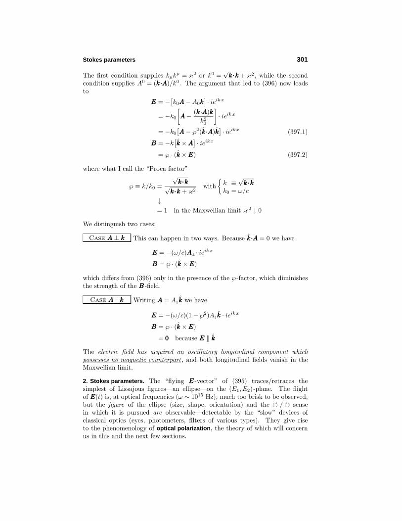
The first condition supplies kµkµ = κ2 or k0 =

√kkk···kkk + κ2, while the second

condition supplies A0 = (kkk···AAA)/k0. The argument that led to (396) now leadsto

EEE = −[k0AAA−A0kkk

]· ieikx

= −k0[AAA− (kkk···AAA)kkk

k20

]· ieikx

= −k0[AAA− ℘2(kkk···AAA)kkk

]· ieikx (397.1)

BBB = −k[kkk ×AAA

]· ieikx

= ℘ · (kkk ×EEE) (397.2)

where what I call the “Proca factor”

℘ ≡ k/k0 =

√kkk···kkk√

kkk···kkk + κ2with

k ≡

√kkk···kkk

k0 = ω/c

↓= 1 in the Maxwellian limit κ

2 ↓ 0

We distinguish two cases:

Case AAA ⊥ kkk This can happen in two ways. Because kkk···AAA = 0 we have

EEE = −(ω/c)AAA⊥· ieikx

BBB = ℘ · (kkk ×EEE)

which differs from (396) only in the presence of the ℘ -factor, which diminishesthe strength of the BBB -field.

Case AAA ‖ kkk Writing AAA = A‖kkk we have

EEE = −(ω/c)(1− ℘2)A‖kkk · ieikx

BBB = ℘ · (kkk ×EEE)

= 000 because EEE ‖ kkk

The electric field has acquired an oscillatory longitudinal component whichpossesses no magnetic counterpart , and both longitudinal fields vanish in theMaxwellian limit.

2. Stokes parameters. The “flying EEE -vector” of (395) traces/retraces thesimplest of Lissajous figures—an ellipse—on the (E1, E2)-plane. The flightof EEE(t) is, at optical frequencies (ω ∼ 1015 Hz), much too brisk to be observed,but the figure of the ellipse (size, shape, orientation) and the / sensein which it is pursued are observable—detectable by the “slow” devices ofclassical optics (eyes, photometers, filters of various types). They give riseto the phenomenology of optical polarization, the theory of which will concernus in this and the next few sections.

302 Light in vacuum

E2

χ√S0

eee2α ψ

eee1 E1

EEE(t)

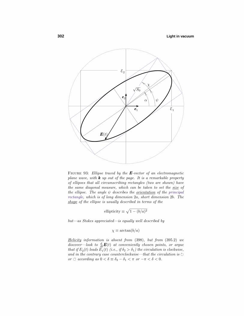
Figure 93: Ellipse traced by the EEE-vector of an electromagneticplane wave, with kkk up out of the page. It is a remarkable propertyof ellipses that all circumscribing rectangles (two are shown) havethe same diagonal measure, which can be taken to set the size ofthe ellipse. The angle ψ describes the orientation of the principalrectangle, which is of long dimension 2a, short dimension 2b. Theshape of the ellipse is usually described in terms of the

ellipticity ≡√

1− (b/a)2

but—as Stokes appreciated—is equally well described by

χ ≡ arctan(b/a)

Helicity information is absent from (398), but from (395.2) wediscover—look to d

dtEEE(t) at conveniently chosen points, or arguethat if E2(t) leads E1(t) (i.e., if δ2 > δ1) the circulation is clockwise,and in the contrary case counterclockwise—that the circulation is or according as 0 < δ ≡ δ2 − δ1 < π or −π < δ < 0.


Eliminating t between equations (395.2) we obtain240

E22 · E2

1 − 2E1E2 cos δ · E1E2 + E21 · E2

2 = E21E

22 sin2 δ (398)

δ ≡ δ2 − δ1 ≡ phase difference

Equations (395.2) provide a parametric description, and (398) an implicitdescription . . . of the ellipse241 shown in Figure 93. Some elementary analyticalgeometry—the details are fun but uninformative, and (since they have nothingspecifically to do with electrodynamics) will be omitted—leads to the followingconclusions:

S0 = E21 + E2

2

sin 2χ = sin 2α · sin δ =2E1E2 sin δ

E21 + E2

2

≡ S3

S0

tan 2ψ = tan 2α · cos δ =2E1E2 cos δ

E21 − E2

2

≡ S2

S1

where S1 ≡ E21 − E2

2

Notice that helicity—which was observed above to be controlled by the signof δ—could as well be said (since E1 and E2 are non-negative) to be controlledby the sign of χ, and that (as is clear from the figure) χ ranges on the restrictedinterval

[− π

2 ,+π2

]. Recasting and extending the results summarized above, we

haveS0 = E2

1 + E22

S1 = E21 − E2

2 = S0 cos 2χ cos 2ψS2 = 2E1E2 cos δ = S0 cos 2χ sin 2ψS3 = 2E1E2 sin δ = S0 sin 2χ

(399)

These equations define the so-called Stokes parameters, which were introducedby G. G. Stokes in to facilitate the discussion of some experimental results.There is reason to think that Stokes himself was unaware of the extraordinarypower of his creation . . .which took nearly a century, and the work of manyhands, to be revealed. Today his lovely idea is recognized to be central toevery classical/statistical/quantum account of the phenomenology of opticalpolarization.

It is evident thatS2

1 + S22 + S2

3 = S20 (400)

and that rotational sense (helicity) can be read from the sign of S3.

240 problem 61.241 problem 62.

304 Light in vacuum

√S0

χ

ψ

S3

S0

2χ S2

2ψS1

Figure 94: Equations (399) serve to associate points on the Stokessphere of radius S0 with centered ellipses of fixed size and all possiblefigures & orientations. Points in the northern hemisphere (S3 > 0)are assigned helicity, points in the southern hemisphere areassigned helicity. In the case S0 = 1 the Stokes sphere becomesthe Poincare sphere.


Henri Poincare () observed that, in view of the structure second stackof equalities in (399), it is natural to place the polarizational states ofelectromagnetic plane waves in one-one association with the points SSS thatcomprise the surface of a sphere of radius S0 in 3-dimensional “Stokes space,”as indicated in Figure 94. It becomes obvious from the figure that specificationof

S0, S1, S2, S3

is equivalent to specification of the intuitively more

immediate parametersS0, ψ, χ

. We need kkk to describe the direction of

propagation and frequency/wavelength of the monochromatic plane wave, butif we have only “slow detectors” to work with then

S0, S1, S2, S3

summarize

all that we can experimentally verify concerning the polarizational state of thewave.242

Reading from Figure 94, we find the polarizational states which correspondto (for example) the axial positions on the Poincare sphere to be thoseillustrated below:

1+1

00

1−1

00

10

+10

10−1

0

100

+1

100−1

It becomes in this light natural to say (with Stokes) of a pair of plane wavesthat they are “oppositely polarized” if and only if their Stokes

SSS ≡

S1

S2

S3

and SSS ≡

S1

S2

S3

vectors point in diametrically opposite directions:

SSS = −λ2SSS

of whichS0 = +λ2S0

242 It is because they relate so directly to the observational realities that Stokesparameters become central to the quantum theory of photon spin. See §2–8 inJ. M. Jauch & F. Rohrlich, The Theory of Photons & Electrons () where,by the way, I was first introduced to this pretty subject.

306 Light in vacuum

is—by (400)—a corollary. From (399) we see that

SSS −→ SSS = −λ2SSS

can, in more physical terms, be described

E1 −→ E1 = +λE2

E2 −→ E2 = −λE1

δ −→ δ = δ

so the “oppositely polarized” associates of

EEE(t) = eee1E1 cosωt+ eee2E2 cos(ωt+ δ)

have the form

EEE(t) = eee1λE2 cos(ωt+ α)− eee2λE1 cos(ωt+ δ + α)

where λ and α are arbitrary. As is intuitively evident, as Fresnel (∼)demonstrated experimentally,243 and as we will soon be in position to prove,oppositely polarized plane waves to not interfere.

I propose now to make more secure the recent claim242 that Stokesparameters pertain directly to the observational properties of plane waves.Energy flux is described (see again page 216) by the

Poynting vector SSS(t) = c(EEE×BBB)

For a plane wave BBB = kkk×EEE

so = cE2(t)kkk

The magnitude of the Poynting vector is given therefore by

S(t) = cE2(t) = cE2

1 cos2 ωt+ E22 cos2(ωt+ δ)

and the intensity of the wave (S(t) averaged over a period τ) by

I ≡ 1τ

∫ τ0

S(t) dt = 12c

E2

1 + E22

So

S0 ≡ E21 + E2

2 = 2cI (401)

can be measured directly by a “J-meter,” i.e., by a photometer that has beenre-scaled so that it displays

J ≡ 2c · (intensity)

243 Augustin Jean Fresnel (–) was an engineer who took up opticswhile a political exile with time on his hands. It was his study of polarizationthat led him to propose that light was to be understood in terms of transversewaves, not the longitudinal waves postulated by Huygens, Young and others.Practical problems of lighthouse design led him to the invention of the Fresnellens and to fundamental contributions to theoretical optics (diffraction).


If an arbitrarily polarized wave

EEEin(t) = eee1E1 cosωt+ eee2E2 cos(ωt+ δ)

is incident upon a ←→ linear polarizer then the exit beam can be described

EEEout(t) = eee1E1 cosωt

so—arguing from (399)—we haveS0

S1

S2

S3

out

=

E21

E21

00

=

12 (S0 + S1)12 (S0 + S1)

00

=

12

12 0 0

12

12 0 0

0 0 0 00 0 0 0

S0

S1

S2

S3

in

We are led thus to these descriptions of the action of some typical polarizers:

←→ polarizer :

S0

S1

S2

S3

out

=

12

12 0 0

12

12 0 0

0 0 0 00 0 0 0

S0

S1

S2

S3

in

(402.1)

polarizer :

S0

S1

S2

S3

out

=

12 − 1

2 0 0− 1

212 0 0

0 0 0 00 0 0 0

S0

S1

S2

S3

in

(402.2)

polarizer :

S0

S1

S2

S3

out

=

12 0 1

2 00 0 0 012 0 1

2 00 0 0 0

S0

S1

S2

S3

in

(402.3)

polarizer :

S0

S1

S2

S3

out

=

12 0 − 1

2 00 0 0 0

− 12 0 1

2 00 0 0 0

S0

S1

S2

S3

in

(402.4)

polarizer :

S0

S1

S2

S3

out

=

12 0 0 1

2

0 0 0 00 0 0 012 0 0 1

2

S0

S1

S2

S3

in

(402.5)

polarizer :

S0

S1

S2

S3

out

=

12 0 0 − 1

2

0 0 0 00 0 0 0

− 12 0 0 1

2

S0

S1

S2

S3

in

(402.6)

Arguing again from (399), we find that the action

EEEin(t) = eee1E1 cosωt+ eee2E2 cos(ωt+ δ)↓

EEEout(t) = eee1e−αE1 cosωt+ eee2e−αE2 cos(ωt+ δ)

308 Light in vacuum

of a neutral filter can be described

neutral filter :

S0

S1

S2

S3

out

= e−2α

1 0 0 00 1 0 00 0 1 00 0 0 1

S0

S1

S2

S3

in

(402.7)

Suppose, now, that we present a plane wave serially to0) a neutral filter F0 with e−2α = 1

2 ,1) a ←→ polarizer F1,2) a polarizer F2,3) a polarizer F3

and in each case use a J-meter to measure the intensity of the output, obtaining

[S0

]out

=

J0 = 12S0 when F0 used

J1 = 12 (S0 + S1) when F1 used



Algebraically deconvolving the output data, we obtain

S0 = 2J0

S1 = 2J1 − 2J0

S2 = 2J2 − 2J0

S3 = 2J3 − 2J0

(403)

Alternative sets of filters would serve as well, but would require some algebraicadjustment at (403). The implication is that

With four suitably selected filters and a photometerone can measure Stokes’ parameters, and thus fullycharacterize the intensity/polarization/helicity of a(coherent monochromatic) plane wave.

3. Mueller calculus. A light beam—modeled, for the moment, as a plane wave—with attributes

kkk, S0, S1, S2, S3

in

is presented to a passive device, from which a beam with attributeskkk, S0, S1, S2, S3

out

emerges. A description of how the output variables depend upon the inputvariables would comprise a characterization of the device. In view of the factthat• mirrors/lenses typically change the direction of the beam, and scatterers

typically spray a beam in multiple directions• some crystals change the frequency of a monochromatic beam• some materials/devices alter the coherence properties of an incident beam,

others alter the degree of polarization (of which more later)

Mueller calculus 309

we recognize that some physical restriction is involved when agree to limit ourconcern to devices that conform to the following scheme:

S0

S1

S2

S3

in

−−−→ device −−−→

S0

S1

S2

S3

out

Since (400) pertains generally to monochromatic plane waves, we see thatfor every such device[

S20 − S2

1 − S22 − S2

3

]out

=[S2

0 − S21 − S2

2 − S23

]in

= 0 (403.1)

while for every passive device (since passive devices are—unlike lasers—notconnected to an external energy source, and therefore may absorb energy from,but cannot inject energy into. . . the transmitted light beam) energy conservationrequires

0 [S0

]out

[S0

]in

(403.2)

A general theory of passive devices would result from an effort to describe thefunctional relationships

Sµout = Dµ(S0in, S1in, S2in, S3in) : µ = 0, 1, 2, 3

permitted by (403). Remarkably, such an effort, if based upon (403.1) alone,would lead back again to the conformal group, which was encountered earlierin quite another connection.244 When (403.2) is brought into play certaingroup elements are excluded: one is left with what might be called the “devicesemigroup.”245

A far simpler theory—which is, however, adequate to most practical needs—is obtained if one imposes the additional assumption that the parametersSµout are linear functions of Sµ in:

S0

S1

S2

S3

in

−−−→ linear passive device −−−→

S0

S1

S2

S3

out

= M

S0

S1

S2

S3

in

One is led then to the linear fragment of the conformal group; i.e., to thecondition (compare (185.2) on pages 129 & 164)

MT jg M = m2 j

g (404.1)

subject to the proviso that one must exclude cases that place one in violationof (403.2). Evidently det M = m4, so in non-singular cases one can state thatM/m is Lorentzian:

M (if non-singular) possesses the structure M = m · /\\\ (404.2)

244 See again Chapter 2, §6. For a brief sketch of the resulting theory of opticaldevices see pages 353–354 in classical electrodynamics ().245 A semigroup is a “group without inversion.”

310 Light in vacuum

remark: One must carefully resist any temptation to concludefrom the design of (404) that the Stokes parameters Sµ transformas the components of a 4-vector. Their Lorentz transformationproperties are inherited—via the definitions (399)—from thoseof the electromagnetic field, and are in fact quite intricate. Thesubject is treated on pages 436 et seq in my electrodynamics().

The idea of using 4×4 matrices to describe the action of linear passive opticaldevices was first developed in a report by Hans Mueller . . .which, however, henever published. Such matrices are called “Mueller matrices,” and their use(discussed below) is the subject matter of the “Mueller calculus.”

The 4×4 matrices encountered in (402.1–6) are readily shown to satisfy

MT jg M = O, which is (404.1) with m = 0 (405)

and to be always in compliance with (403.2).246 So each is a Mueller matrix.Each is found, moreover, to possess247 the “projection property”248

M2 = M (406)

Calculation shows, moreover, that in each case

det(M− λI) = λ3(λ− 1) (407)

so

MSin = 0 has three linearly independent solutions;the device extinguishes such beams

MSin = Sin has but one; the device is transparent tosuch beams (scalar multiples of one another)

example : Noting that 32 + 42 + 122 = 132 let us, by contrivance, take

Sin =

133412

and let us take M to be the Mueller matrix of (402.1) that describes the actionof a ←→ polarizer. Then (by quick calculation)

246 problem 63.247 problem 64.248 From (406) it follows, by the way, that (det M)2 = det M whence

det M = 1 if M is the trivial projector I

0 otherwise

The zero on the right side of (405) can be therefore be looked upon as a forcedconsequence of projectivity.


Sout = MSin =

8800

, projected component of

133412

The exit beam is 100% ←→ polarized, but dimmer:

S0out = 8 < S0in = 13

A second pass through the device (second such projection) has no effect (thatbeing the upshot of M

2 = M):

M

8800

=

8800

To describe the action of an arbitrary polarizer : let σσσ be an arbitrary unit3-vector and construct

M(σσσ) ≡ 12 ·

1 σ1 σ2 σ3

σ1 σ1σ1 σ1σ2 σ1σ3



(408.1)

One can show249 that M(σσσ) satisfies (405/6/7) and that

M(σσσ)

1σ1

σ2

σ3

=

1σ1

σ2

σ3

(408.2)

MoreoverM(−σσσ)M(+σσσ) = O : all σσσ (409)

which supplies neat support for Stokes’ claim (page 305) that diametricallyopposite points on the Stokes sphere refer to “opposite polarizations,” andconforms precisely to the pattern evident when one compares (402.2) with(402.1), (402.4) with (402.3), (402.6) with (402.5). In the case

σσσ =

1

00

Equation (409) might be notated

M(↑↓)M(←→) = O

249 problem 65.

312 Light in vacuum

and interpreted to express the familiar fact that no light passes through crossedpolarizers.

Suppose, however, we were to interpose (between M(↑↓) and M(←→)) a thirddevice: let it be (say) the linear polarizer represented (see again Figure 94) by

M(ψ) ≡M(σσσ) with σσσ =

cos 2ψ

sin 2ψ0

With the assistance of Mathematica we compute

M(↑↓)M(ψ)M(←→) =

18 sin2 2ψ 1

8 sin2 2ψ 0 0− 1

8 sin2 2ψ − 18 sin2 2ψ 0 0

0 0 0 00 0 0 0

= O

which illustrates the basis of an experimental technique standard to microscopyand engineering: one places a microscope slide or the stressed Lucite model of amachine part between crossed polarizers, and examines the transmitted image.

The preceding calculation also illustrates the central idea of the “Muellercalculus”: To determine the net effect of cascaded optical devices one simplymultiplies the corresponding Mueller matrices.

“Optical devices” exist in considerable variety. At (402.7) we encounteredthe Mueller matrices

M = e−2α · I (410)

that describe the action of “neutral filters.” Such a device is transparentat α = 0, and becomes progressively more absorptive (optically dense) as αincreases.

Mueller matrices of major practical importance arise if at (404.2) we setm = 1 and assume M = /\\\ to have (see again (208) on page 155) the rotationaldesign

M =

1 0 0 000 R

0

(411)

R ≡ exp

2θ

0 −σ3 σ2

σ3 0 −σ1

−σ2 σ1 0

: a rotation matrix

Such an M leaves S0 invariant (no absorption) but causes

SSS ≡

S1

S2

S3


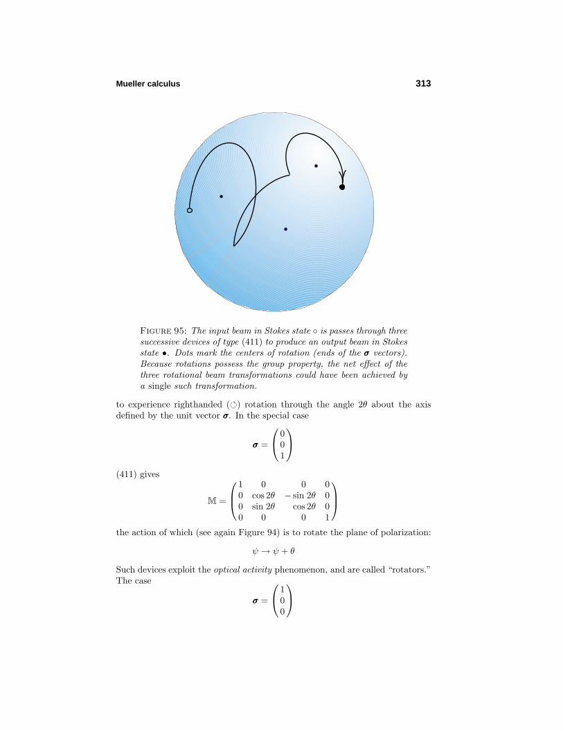
Figure 95: The input beam in Stokes state is passes through threesuccessive devices of type (411) to produce an output beam in Stokesstate •. Dots mark the centers of rotation (ends of the σσσ vectors).Because rotations possess the group property, the net effect of thethree rotational beam transformations could have been achieved bya single such transformation.

to experience righthanded () rotation through the angle 2θ about the axisdefined by the unit vector σσσ. In the special case

σσσ =

0

01

(411) gives

M =

1 0 0 00 cos 2θ − sin 2θ 00 sin 2θ cos 2θ 00 0 0 1

the action of which (see again Figure 94) is to rotate the plane of polarization:

ψ → ψ + θ

Such devices exploit the optical activity phenomenon, and are called “rotators.”The case

σσσ =

1

00

314 Light in vacuum

gives

M =

1 0 0 00 1 0 00 0 cos 2θ − sin 2θ0 0 sin 2θ cos 2θ

which achievesδ → δ + 2θ

Such devices are called “compensators” or “phase shifters.” It is clear thatMueller matrices of type (411) are non-singular: M

–1 is again a Mueller matrix,which means that the action of such a device could be undone by a suitablychosen second such device. Projection, on the other hand, is a non-invertibleoperation: the action of a polarizer, when undone by subsequent polarizers,always entails attenuation of the beam. To illustrate the point, we return tothe example of page 312 and by computation find that

M(←→)M(ψ)M(←→) = 12 cos4 ψ ·M(←→)

Looking back again to (404.2), it becomes natural in view of the foregoingto assign /\\\ the “boost” design of (209), writing

M = m·

γ β1γ β2γ β3γβ1γ 1+(γ−1)β1β1/β

2 (γ−1)β1β2/β2 (γ−1)β1β3/β

2

β2γ (γ−1)β2β1/β2 1+(γ−1)β2β2/β

2 (γ−1)β2β3/β2

β3γ (γ−1)β3β1/β2 (γ−1)β3β2/β

2 1+(γ−1)β3β3/β2

where the β ’s are “device parameters” that have now nothing to do with velocity .Immediately

S0out = mγ(S0in + βββ ···SSSin)

SSSin = S0in SSSin by (400)

= mγ(1 + βββ ··· SSSin)S0in

= mγ(1 + β cosω)S0in : ω is the angle between βββ and SSSin

so to achieve universal compliance with the passivity condition (403.2) we musthave

0 < m √

1−β1+β 1

where it is understood that 0 β < 1. It is not at all difficult to show of suchMueller matrices that though M

–1 exists—and is, in fact, easy to describe

[m/\\\(βββ)]–1 = m–1/\\\(−βββ)

—it stands in violation of the passivity condition, so cannot be realized bya passive device. On pages 361/2 of some notes already cited244 I exploresome of the finer details of this subject, and argue that it should be possible

Partial polarization 315

to mimic 4-dimensional relativity (composition of non-colinear boosts, Thomasprecession, etc.) by experiments performed on a linear optical bench!

In some respects more elegantly efficient—but in other physical respectsmore limited—than the Mueller calculus is the “Jones calculus,” devised byR. Clark Jones one summer in the early ’s while he was employed in thelaboratory of Edwin Land as a Harvard undergraduate. In Jones’ formalismStokes’ parameters are folded into the design of a complex 2-vector, and devicesare represented by complex 2×2 matrices. The formalism is developed inelaborate detail in my “Ellipsometry” () and in the literature cited there,but it would take us too far afield to attempt to treat the subject here.

4. Partially polarized plane waves. The “plane waves” considered thus far arehighly idealized abstractions: they• are of infinite temporal duration• are of infinite spatial extent . . . and therefore• carry infinite energy and momentum, and moreover• are spatially/temporally perfectly coherent.

But so also—and in much the same way—is the Euclidean plane an idealizedabstraction. Euclidean geometry becomes relevant to physical geometry onlyin contexts (very numerous indeed!) in which it is sensible to conflate the localgeometry of the curved surface with the local geometry of the tangent plane. Soit is in classical electrodynamics: ideas borrowed from the idealized physics ofplane waves become relevant to the physics of realistic radiation fields only aslocal approximants,250 and can be expected to lose their utility “in the large,”as also in the vicinity of charges, caustics, “kinks” in the field.

But radiation fields the gross properties of which display any degree ofspatial/temporal variability cannot be precisely monochromatic. We expectnatural fields to acquire also some degree of spatial/temporal incoherence fromthe radiation production mechanism, whatever it might be. We are led thusto the concept of a quasi-monochromatic plane wave—led, that is, to thereplacement

EEE(t) =eee1E1e

iδ1 + eee2E2eiδ2

eiωt (395)

↓EEE(t) =

eee1E1(t)eiδ1(t) + eee2E2(t)eiδ2(t)

eiωt (412)

where ω sets the nominal frequency and E1(t), E2(t), δ1(t) and δ2(t) are assumedto change• slowly with respect to eiωt but (in typical cases)• rapidly with respect to the response time of our photometers.

250 Beware! Plane waves are, in one critical respect, not representative of thetypical local facts. I refer to the circumstance that, while EEE ⊥ BBB is charac-teristic of plane waves, it is not a property of fields in general (superimposedplane waves). See below, page 332.

316 Light in vacuum

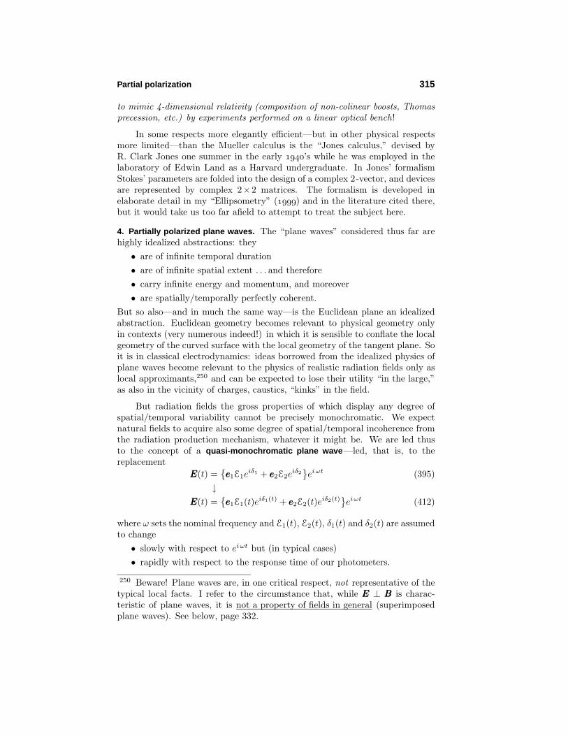
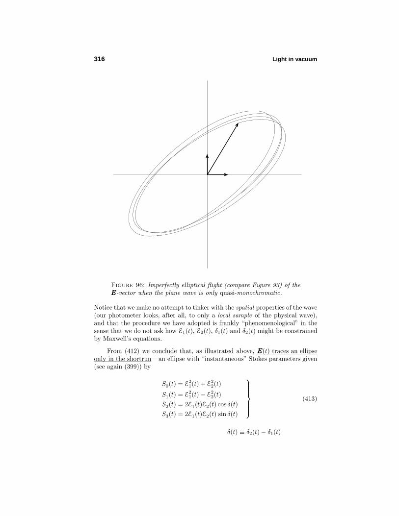
Figure 96: Imperfectly elliptical flight (compare Figure 93) of theEEE-vector when the plane wave is only quasi-monochromatic.

Notice that we make no attempt to tinker with the spatial properties of the wave(our photometer looks, after all, to only a local sample of the physical wave),and that the procedure we have adopted is frankly “phenomenological” in thesense that we do not ask how E1(t), E2(t), δ1(t) and δ2(t) might be constrainedby Maxwell’s equations.

From (412) we conclude that, as illustrated above, EEE(t) traces an ellipseonly in the shortrun—an ellipse with “instantaneous” Stokes parameters given(see again (399)) by

S0(t) = E21(t) + E2

2(t)

S1(t) = E21(t)− E2

2(t)S2(t) = 2E1(t)E2(t) cos δ(t)S3(t) = 2E1(t)E2(t) sin δ(t)

(413)

δ(t) ≡ δ2(t)− δ1(t)


The ellipse jiggles about, constantly changing is figure/orientation, in a mannerdetermined by the (let us say steady) statistical properties of the wave. Thefunctions E1(t),E2(t) and δ(t)—whence also S0(t), S1(t), S2(t) and S3(t)—have,in other words, assumed the character of random variables. Our filters and(slow) J-meters, used as described on page 308, supply information not aboutthe functions Sµ(t) but about their mean values:

Sµ ≡ 〈Sµ(t)〉 ≡ 1T

∫ T

0

Sµ(t) dt :

T might refer to the responsetime of the instrument

Proceeding in this light from (403) and (413) we have

S0 = 2J0 = 〈E21〉+ 〈E2

2〉S1 = 2J1 − 2J0 = 〈E2

1〉 − 〈E22〉

S2 = 2J2 − 2J0 = 2〈E1E2 cos δ〉S3 = 2J3 − 2J0 = 2〈E1E2 sin δ〉

(414)

Evidence that Stokes’ parameters are, if not by initial intent, neverthelesswonderfully well-adapted to discussion of the dominant statistical properties ofphysical lightbeams emerges from the following little argument: working from(414) we have

S20 = 〈E2

1〉2 + 2〈E21〉〈E2

2〉+ 〈E22〉2 (415.1)

S21 + S2

2 + S23 = 〈E2

1〉2 − 2〈E21〉〈E2

2〉+ 〈E22〉2 + 〈2E1E2 cos δ〉2 + 〈2E1E2 sin δ〉2

= S20 + 4

〈E1E2 cos δ〉2 + 〈E1E2 sin δ〉2 − 〈E2

1〉〈E22〉

(415.2)

But if x and y are any random variables (however distributed) then from〈(λx + y)2〉 = λ2〈x〉2 + 2λ〈xy〉 + 〈y〉2 0 (all λ) it follows that in all cases〈xy〉2 〈x2〉〈y2〉, so we have

〈E1E2 cos δ〉2 〈E21〉〈E2

2 cos2 δ〉〈E1E2 sin δ〉2 〈E2

1〉〈E22 sin2 δ〉

giving

S21 + S2

2 + S23 ≤ S2

0 + 4〈E2

1〉〈E2(cos2 δ + sin2 δ)2〉 − 〈E21〉〈E2

2〉︸︷︷︸

0

We are led thus to the important inequality

S20 − S2

1 − S22 − S2

3 0 (416)

318 Light in vacuum

with—according to (400)—equality if (but not only if!) the beam is literallymonochromatic. Looking back again to Figure 94, we see that (416) serves toplace the vector

SSS ≡

S1

S2

S3

inside the Stokes sphere of radius S0, and that SSS reaches all the way to thesurface of the Stokes sphere if and only if the beam is, in a fairly evident sense,statistically equivalent to a monochromatic beam.

If E1, E2 and δ are statistically independent random variables then we canin place of (414) write

S0 = 〈E21〉+ 〈E2

2〉S1 = 〈E2

1〉 − 〈E22〉

S2 = 2〈E1〉〈E2〉〈cos δ〉S3 = 2〈E1〉〈E2〉〈sin δ〉

If, moreover, all δ -values are equally likely, then 〈cos δ〉 = 〈sin δ〉 = 0, and wehave S2 = S3 = 0. If, moreover, 〈E1〉 = 〈E2〉 then S1 = 0. The resulting beam

1000

is said to be unpolarized : SSS = 000

It becomes on this basis natural to introduce the

“degree of polarization” P ≡

√S2

1 + S22 + S2

3

S0: 0 P 1 (417)

and to write

S0

S1

S2

S3

=

PS0

S1

S2

S3

+

(1− P )S0

000

= 100% polarized component + unpolarized component

When an unpolarized beam is presented to (for example) the linear polarizer of(402.1) one obtains

S0

S1

S2

S3

in

−−−−−−−−−−−−−−−−→linear polarizer at 0

S0

S1

S2

S3

out

=

12

12 0 0

12

12 0 0

0 0 0 00 0 0 0

S0

000

in

=

12S012S0

00


HerePin = 0 : the entry beam is unpolarized, butPout = 1 : the exit beam is 100% polarized

And when the exit beam is presented to a second linear polarizer, described bythe M(ψ) of page 312, one obtains251 the “Law of Malus”:

output intensityinput intensity

= 14 (1 + cos 2ψ) = 1

2 cos2 ψ

A quasi-monochromatic beam is said to be

unpolarizedpartially polarized

completely polarized

according as

0 = P

0 < P < 1P = 1

An unpolarized beam necessarily is polarized in the shortrun, but in the longerterm the EEE -vector traces an orientation-free scribble. Partial polarizationresults when the scribble is somewhat oriented (fuzzy): this requires that E1(t),E2(t), δ1(t) and δ2(t) more somewhat in concert; i.e., that they be statisticallycorrelated . It is important to note that the numbers Sµ provide a veryincomplete description of the beam statistics, and that even complete knowledgeof the statistical properties of the beam would leave the actual t -dependence ofEEE indeterminate. Many beams are—even in the case of complete polarization—consistent with any prescribed/measured set of Sµ-values.

We are by those remarks into position to appreciate the import of Stokes’

Principle of Optical Equivalence: Lightbeams with identicalStokes parameters are “equivalent” in the sense that theyinteract identically with devices which detect or alter theintensity and/or polarizational state of the incident beam.

and the depth of his insight into the physics of light. But one does not sayof objects that they are, in designated respects, “equivalent” unless there existother respects—whether overt or covert—in which they are at the same timeinequivalent; implicit in the formulation of Stokes’ principle is an assertionthat physical light beams possess properties beyond those to which the Stokesparameters allude, properties to which photometer-like devices are insensitive.There are many ways to render a page gray with featureless squiggles, manyways to assemble an unpolarized light beam. What such beams, such statisticalassemblages share is, according to (414), not “identity” but only the propertythat a certain quartet of numbers arising from their low-order moments andcorrelation coefficients are equi-valued.

251 problem 66. Etienne Louis Malus (–) was a French engineer/physicist.

320 Light in vacuum

We have, in effect, been alerted by Stokes to the existence of a “statisticaloptics”—to the possibility that instruments (more subtle in their action thanphotometers) might be devised which are sensitive to higher moments of anincident optical beam. And we have been alerted to the possible existenceand potential usefulness of an ascending hierarchy of “higher order analogs” ofthe parameters that bear Stokes’ name, formal devices that serve to capturesuccessively more refined statistical properties of optical beams. Examinationof the literature252 shows all those expectations to be borne out by fairly recentdevelopments. It becomes interesting in the light of these remarks to recallthe title of the paper in which the Stokes parameters were first described:“On the composition and resolution of streams of polarized light from differentsources” (Trans. Camb. Phil. Soc. 9, 399 (1852)). Stokes brought the theoryof physical light beams to a state somewhat analogous to that encounteredin thermodynamics, where a few operationally defined variables mask a richtime-dependent microphysics, yet serve to support a formalism which is—surprisingly—closed/self-consistent/complete . . . and which accounts accuratelyfor the phenomenological facts.

Already on page 318 we began to accumulate evidence that the Muellercalculus is as “robust” as the Stokes formalism upon which it is based. To ourformer population of Mueller matrices M it might now seem appropriate to add(for example)

M ≡

1 0 0 00 e−u 0 00 0 e−u 00 0 0 e−u

: u 0 (418)

which evidently describes the action of an isotropic depolarizer , where theadjective refers to isotropy not in physical space but in Stokes space. Theinteresting point—which stands as an open invitation to formal/physicalinvention—is that the M described above does not satisfy the fundamentalMueller condition (404.1). Relatedly: I am informed by Morgan Mitchell, myoptical colleague, that while active “polarization scramblers” do exist, a “passivedepolarization device” would be a “tall order.” 253, 254

5. Optical beams. Listed at the beginning are several respects in which “planewaves are highly idealized abstractions.” With the introduction of the notionof “quasi-monochromaticity” we were able to introduce an element of realisminto the discussion, but• infinite temporal duration• infinite spatial extent• infinite energy/momentum

252 See, for example, E. L. O’Neill, Introduction to Statistical Optics ();J. W. Simmons & M. J. Guttmann, States, Waves and Photons: A ModernIntroduction to Light (); C. Brosseau,Fundamentals of Polarized Light: AStatistical Optics Approach ().253 problem 67.254 problem 68.

Optical beams 321

Figure 97: Representation of the function ϕ(t, x, 0, z) described at(419) below. The Gaussian wavepacket glides rigidly, as indicatedby the arrow. It is temporally confined, but spatially unconfined.

are unphysical abstractions that survived untouched in the ensuing discussionof beam statistics and imperfect polarization. Temporal confinement is fairlyeasy to achieve, as the following remark makes clear:

Write ei(kct+0x+0y−kz) to describe a plane wave running up the z-axis.Write

ϕ(t, x, y, z) =∫ +∞

−∞f(k)eik(c t−z) dk

=∫ +∞

−∞g(ω)eiω( t−z/c) dω

to describe a weighted superposition of such waves. Take g(ω) to have, inparticular, the form of a normalized Gaussian centered at Ω:

g(ω) ≡ 1√2πTe−

12 T 2(ω−Ω)2 : T > 0 has the physical dimension of time

↓= δ(ω − Ω) as T ↑ ∞

Then

ϕ(t, x, y, z) =∫ +∞

−∞1√2πTe−

12 T 2(ω−Ω)2eiω( t−z/c) dω

= e−12 T −2(t−z/c)2 · eiΩ(t−z/c) (419)

↓= eiΩ(t−z/c) as T ↑ ∞

The physical (i.e., the real) part of the expression on the right side of (419) isplotted in Figure 97.

322 Light in vacuum

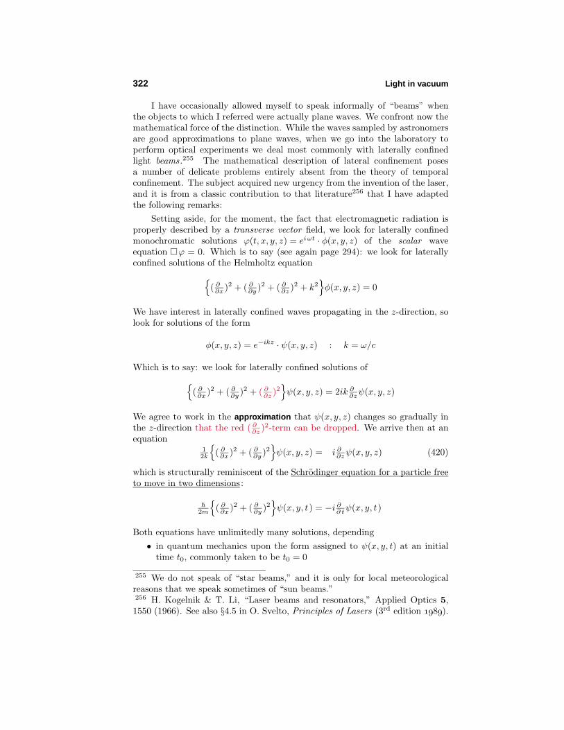
I have occasionally allowed myself to speak informally of “beams” whenthe objects to which I referred were actually plane waves. We confront now themathematical force of the distinction. While the waves sampled by astronomersare good approximations to plane waves, when we go into the laboratory toperform optical experiments we deal most commonly with laterally confinedlight beams.255 The mathematical description of lateral confinement posesa number of delicate problems entirely absent from the theory of temporalconfinement. The subject acquired new urgency from the invention of the laser,and it is from a classic contribution to that literature256 that I have adaptedthe following remarks:

Setting aside, for the moment, the fact that electromagnetic radiation isproperly described by a transverse vector field, we look for laterally confinedmonochromatic solutions ϕ(t, x, y, z) = eiωt · φ(x, y, z) of the scalar waveequation ϕ = 0. Which is to say (see again page 294): we look for laterallyconfined solutions of the Helmholtz equation

( ∂∂x )2 + ( ∂

∂y )2 + ( ∂∂z )2 + k2

φ(x, y, z) = 0

We have interest in laterally confined waves propagating in the z-direction, solook for solutions of the form

φ(x, y, z) = e−ikz · ψ(x, y, z) : k = ω/c

Which is to say: we look for laterally confined solutions of( ∂

∂x )2 + ( ∂∂y )2 + ( ∂

∂z )2ψ(x, y, z) = 2ik ∂

∂zψ(x, y, z)

We agree to work in the approximation that ψ(x, y, z) changes so gradually inthe z-direction that the red ( ∂

∂z )2-term can be dropped. We arrive then at anequation

12k

( ∂

∂x )2 + ( ∂∂y )2

ψ(x, y, z) = i ∂

∂zψ(x, y, z) (420)

which is structurally reminiscent of the Schrodinger equation for a particle freeto move in two dimensions:

2m

( ∂

∂x )2 + ( ∂∂y )2

ψ(x, y, t) = −i ∂

∂ tψ(x, y, t)

Both equations have unlimitedly many solutions, depending• in quantum mechanics upon the form assigned to ψ(x, y, t) at an initial

time t0, commonly taken to be t0 = 0

255 We do not speak of “star beams,” and it is only for local meteorologicalreasons that we speak sometimes of “sun beams.”256 H. Kogelnik & T. Li, “Laser beams and resonators,” Applied Optics 5,1550 (1966). See also §4.5 in O. Svelto, Principles of Lasers (3rd edition ).

Optical beams 323

• in beam theory upon the form assigned to ψ(x, y, z) at some prescribedaxial point z0; we will find it convenient to take z0 = 0.

To illustrate the point, the authors of quantum texts257 often take ψ(x, y, t0)to be Gaussian

ψ(x, y, 0) = Ae−a(x2+y2)

and by one or another of the available computational techniques obtain

ψ(x, y, 0) −−−−→t

ψ(x, y, t) = A 11+i(t/T ) exp

− a(x2+y2)

1+i(t/T )

: T ≡ m/2a

which they use to demonstrate the characteristic temporal diffusion of initiallylocalized quantum states. Exactly the same mathematics lies at the base of the“theory of Gaussiam beams.” Suppose it to be the case that

ψ(x, y, z) = Be−a(x2+y2) at z = 0

The exact solution of (420) is given then at other axial points z by258

ψ(x, y, z) = B 11−iz/Z e

−a(x2+y2)/(1−iz/Z) : Z ≡ k/2a

= B 11+(z/Z)2 [1 + i(z/Z)] exp

−ar2 1

1+(z/Z)2 [1 + i(z/Z)]

[1 + i(z/Z)] =√

1 + (z/Z)2 eiΦ with Φ ≡ arctan(z/Z)

= B√1+(z/Z)2

exp−ar2 1

1+(z/Z)2

exp

i[Φ(z)− ar2 z/Z

1+(z/Z)2

]r2 ≡ x2 + y2

We are brought thus to a beam of the design

ϕ(t, x, y, z) ∼ 1ρ(z) exp

−

[r

ρ(z)

]2·ei[ωt−kz+Φ(z)−(r/ρ)2(z/Z)

](421)

where

ρ(z) ≡√

1 + (z/Z)2

adescribes the “spot radius” at z

Evidently

ρmin ≡ ρ0 = ρ(0) =√

1/a : called the “beam waist”

and at this point the a-notation—a relic of Griffiths’ discussion of anothersubject—has outworn its usefulness: we agree henceforth to write 1/ρ2

0 in placeof a. In this new notation we have

ρ(z) = ρ0

√1 + (z/Z)2 i.e., (ρ/ρ0)2 − (z/Z)2 = 1 (422)

257 See, for example, David Griffiths, Introduction to Quantum Mechanics(), page 50: Problem 2.22.258 problem 69.

324 Light in vacuum

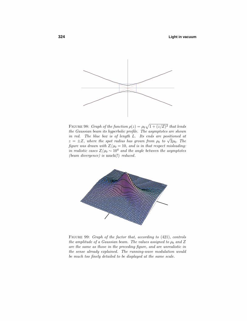
Figure 98: Graph of the function ρ(z) = ρ0

√1 + (z/Z)2 that lends

the Gaussian beam its hyperbolic profile. The asymptotes are shownin red. The blue box is of length L. Its ends are positioned atz = ±Z, where the spot radius has grown from ρ0 to

√2ρ0. The

figure was drawn with Z/ρ0 = 10, and is in that respect misleading:in realistic cases Z/ρ0 ∼ 104 and the angle between the asymptotes(beam divergence) is much(!) reduced .

Figure 99: Graph of the factor that, according to (421), controlsthe amplitude of a Gaussian beam. The values assigned to ρ0 and Zare the same as those in the preceding figure, and are unrealistic inthe sense already explained. The running-wave modulation wouldbe much too finely detailed to be displayed at the same scale.

Optical beams 325

which shows that the growth of the spot radius is hyperbolic (see Figure 98 &Figure 99), with asymptotes

ρasymptotic = ±(ρ0/Z)z

the slopes of which are typically very shallow: from the definition

Z ≡ 12L ≡ kρ2

0/2 = πρ20/λ

we havebeam waist = 0.3989

√Lλ

beam divergence = 0.7978√λ/L

(423)

where the numerics arise from√

1/2π and√

2/π respectively. In a typical caseL ∼ 1 meter and λ ∼ 7.0×10−7 meter, giving

beam waist = 0.33 mm

beam divergence = 6.67×10−4 (dimensionless)

Such a beam must travel about 15 meters for the spot radius to grow to 1 cm.

Looking back again to (421), we set r = 0 and find that the

axial phase at z = ωt− kz + arctan(z/Z)

Arguing from ddt (axial phase at z) = 0 we compute

phase velocity at z =[k − Z

Z2+z2

]–1 · ω=

[1− Zλ

2π(Z2+z2)

]–1 · c by Z/k = Zλ/2π = 12ρ

20

=

1 + λ2πZ +

(λ

2πZ

)2 + · · ··c c at z = 0

↓= c as z →∞

—the interesting point being that as z becomes large the axial phase velocityapproaches c from above. Looking next to the geometry of the near-axialequiphase surfaces, we study

kz − arctan(z/Z) +r2

ρ20[1 + (z/Z)2]

(z/Z) = kz0 − arctan(z0/Z) (424)

where z0 marks the point at which the surface in question intersects the z-axis.Taking both r2 and z0 − z to be small and asking Mathematica to develop thearctan as a power series in (z − z0), we obtain

r2

ρ20[1 + (z0/Z)2]

(z0/Z) =k − 1

Z[1 + (z0/Z)2]

(z0 − z) + · · · (425)

Define R in such a way that

k2R≡ 1

ρ20[1 + (z0/Z)2]

(z0/Z)

which is to say: let R ≡ z[1 + (Z/z)2], so that the expression on the left side of

326 Light in vacuum

Figure 100: Equiphase contours, taken from the expression on theleft side of (424).

(425) can be written kr2/2R. Next, notice that

1Z[1 + (z0/Z)2]

<1Z

= 2L π

2λ

= k

so the second term in braces can be abandoned, giving (see Figure 100)

z0 − z = (1/2R)(x2 + y2) :

parabola-of-revolution, openingto the left, with apex at z0

(425)

ThatR = radius of curvature at the apex

follows from the observations (i) that

[z − (z0 −R)]2 + x2 + y2 = R2 (426)

describes a sphere of radius R that is centered on the z-axis and intersects thataxis at z = z0 and z = z0 − 2R, and (ii) that expansion of (426) gives back(425) if a small (z0 − z)2-term is abandoned. This information might be usedto design the concave mirrors placed at the ends of a “Gaussian laser.”

The Gaussian beam discussed above can be used as the “seed” from whichto grow an infinite population of “Gaussian beams of higher order.” These (atleast those of lower order) are of physical importance when taken individually,and collectively enable one (by weighted superposition) to fabricate beams ofunlimited variety. The generative idea is quite elementary

If ϕ is a solution of ϕ = 0 and if D is a differentialoperator that commutes with

D = D

then so also is Dϕ a solution.

but must be adapted to the approximation scheme that was seen on page 322to lie at the base of Gaussian beam theory: we write

ϕ(t, x, y, z) = ei(ω t−kx) · ψ(x, y, z)

Optical beams 327

and require that ψ be an exact solution of the “Schrodinger equation”259( ∂

∂x )2 + ( ∂∂y )2

ψ(x, y, z) = i(4Z/ρ2

0)∂∂zψ(x, y, z) (427)

Taking from page 323 the demonstrably exact solution

ψ00 = ρ01

ρ0[1 − iz/Z]exp

− x2 + y2

ρ20[1 − iz/Z]

—which by ρ0[1− iz/Z] = ρ0

√1 + (z/Z)2 e−i arctan(z/Z) ≡ ρ(z)e−iΦ(z) can also

be written

= ρ01

ρ(z)eiΦ(z) · exp

−

[ x

σ(z)

]2

−[ y

σ(z)

]2

σ(z) ≡√ρ0ρ(z) e−i 1

2 Φ

= ρ01ρe

iΦ · e−ξ2−η2: ξ ≡ x/σ and η ≡ y/σ

—as our “seed,” we harvest this fairly natural fruit:

ψmn ≡(−ρ0

∂∂x

)m(−ρ0

∂∂y

)nψ00

= ρ01ρe

iΦ(−ρ0

1σ

∂∂ξ

)m(−ρ0

1σ

∂∂η

)ne−ξ2−η2

= ρ01ρe

iΦ(ρ0

1σ

)m+n(− ∂

∂ξ

)m(− ∂

∂η

)ne−ξ2−η2

=(ρ0

1ρ

)1+ 1

2 (m+n) ei[1+ 12 (m+n)]ΦHm(ξ)Hn(η) · e−ξ2−η2

(428)

In the final line we have recalled260 Rodrigues’ construction

Hm(ξ) = eξ2(− ∂∂ξ

)me−ξ2

of the Hermite polynomials:

H0(ξ) = 1H1(ξ) = 2ξH2(ξ) = 4ξ2 − 2H3(ξ) = 8ξ3 − 12ξH4(ξ) = 16ξ4 − 48ξ2 + 12

...

That the functions ψmn constructed in this way do in fact exactly satisfy (427)can be demonstrated (for small m, n) by Mathematica -assisted calculation, butthat they must do so follows transparently from the observation that

∂∂x and ∂

∂y commute with

( ∂∂x )2 + ( ∂

∂y )2− i(4Z/ρ2

0)∂∂z

259 This is just (420) with k → 2aZ = 2Z/ρ20.

260 See, for example, Chapter 24 in J. Spanier & K. B. Oldham, An Atlas ofFunctions ().

328 Light in vacuum

The Gaussian factor

e−ξ2−η2= exp

−x2 + y2

ρ2(z)[1 + i(z/Z)]

is a shared feature of all the ψmn-functions, which give rise therefore to identicalpopulations of equiphase surfaces (Figure 100). Using Mathematica’s

HermiteH[n,x]

command to evaluate the complex prefactors

gmn(x, y) ≡(ρ0

1ρ

)1+ 1

2 (m+n) ei[1+ 12 (m+n)]ΦHm

( x√ρ0ρe

i 12 Φ

)Hn

( y√ρ0ρe

i 12 Φ

)in some low-order cases, we find

g00 = (ρ0/ρ)eiΦ

g10 = (ρ0/ρ)2(x/ρ)e2iΦ

...g20 = (ρ0/ρ)4(x/ρ)2e3iΦ − 2(ρ0/ρ)2e2iΦ

g11 = (ρ0/ρ)2(x/ρ)

2(y/ρ)

e3iΦ

...g30 = (ρ0/ρ)8(x/ρ)3e4iΦ − 12(ρ0/ρ)2(x/ρ)e3iΦ

g21 = (ρ0/ρ)4(x/ρ)22(y/ρ)e4iΦ − 2(ρ0/ρ)2e3iΦ

2(y/ρ)

...

The red terms depart from the result asserted by Kogelnik & Li and quoted bySvelto256:

gmn = (ρ0/ρ)Hm(x/ρ)Hn(y/ρ) ei[1+m+n]Φ

Their results261 and mine are, however, in precise agreement at z = 0, whereρ = ρ0 and Φ = 0 give

ψmn(x, y, 0) = Hm(x/ρ0)Hn(y/ρ0) exp−x2 + y2

ρ20

This striking result acquires special interest from the orthogonality relation∫ +∞

−∞Hµ(u)Hν(u)e−u2

du =√πµ!2µδµν

261 . . .which are not incorrect (as I for awhile supposed) but refer to a distinctpopulation of beam modes: the point is developed in §§3 & 4 of a companionessay “Toward an exact theory of lightbeams” ().

Optical beams 329

For if we introduce the “normalized Gaussian beam functions”

Ψmn(x, y, z) ≡ 1ρ0

√m!2mn!2nπ

ψmn(x, y, z)

then we have∫ +∞

−∞

∫ +∞

−∞Ψµν(x, y, 0)Ψmn(x, y, 0) exp

x2 + y2

ρ20

dxdy = δµmδνn

which we can use to evaluate the coefficients cmn that enter into the description

ψ(x, y, 0) =∑m,n

cmnΨmn(x, y, 0)

of beam structure at the waist . We then write

ϕ(t, x, y, z) = ei(ωt−kz) ·∑m,n

cmnΨmn(x, y, z) (429)

=∑

modes

Gaussian beams of various “modes” (identified by m,n)

to describe the generalized Gaussian beam possessing that prescribed structureat the waist.

Physically more realistic beam models would be obtained if we• used the mechanism described on page 321 to turn the beam on/off

(this would entail loss of strict monochromaticity)• constructed statistical linear combinations of such beams.

But the beams thus constructed could not possibly describe laser beams: theyare scalar beams (“acoustic” beams), whereas physical laser beams must beendowed with the transverse vectorial properties known to be characteristic ofall electromagnetic radiation. This is a circumstance we were content to setaside on page 322, but would like now to find some way to accommodate. Iinvite you to turn on Mathematica and follow along. . .

Exponential solutions of the “Schrodinger equation” (427) can be described

expi[− px− qy +

p2 + q2

4Z/ρ20

z]

: all real p, q

and minimal tinkering leads to the discovery that∫∫ +∞

−∞

ρ20

4π e− 1

4 ρ20(p

2+q2) · expi[− px− qy +

p2 + q2

4Z/ρ20

z]

dpdq (430.1)

=1

[1 − iz/Z]exp

− x2 + y2

ρ20[1 − iz/Z]

= ψ00(x, y, z) of page 327

330 Light in vacuum

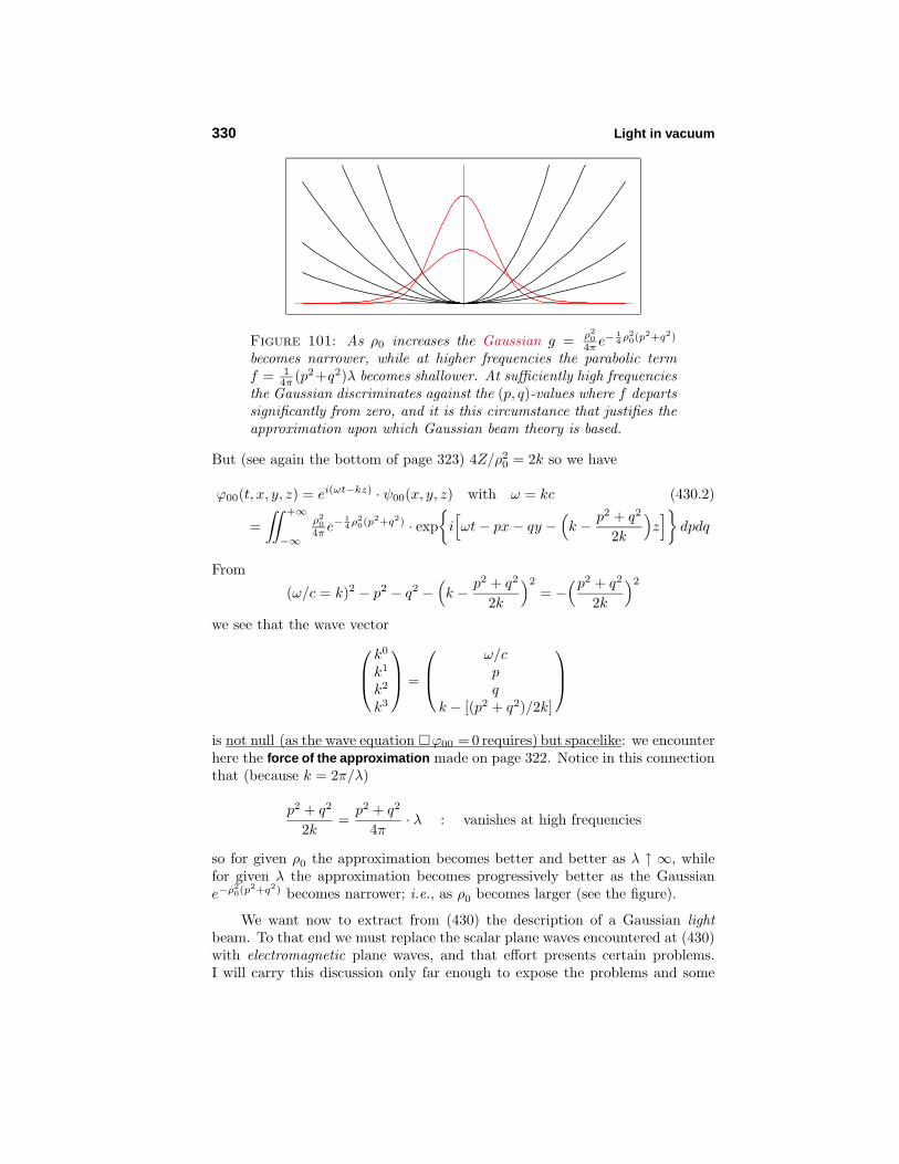
Figure 101: As ρ0 increases the Gaussian g = ρ20

4π e− 1

4 ρ20(p

2+q2)

becomes narrower, while at higher frequencies the parabolic termf = 1

4π (p2+q2)λ becomes shallower. At sufficiently high frequenciesthe Gaussian discriminates against the (p, q)-values where f departssignificantly from zero, and it is this circumstance that justifies theapproximation upon which Gaussian beam theory is based.

But (see again the bottom of page 323) 4Z/ρ20 = 2k so we have

ϕ00(t, x, y, z) = ei(ωt−kz) · ψ00(x, y, z) with ω = kc (430.2)

=∫∫ +∞

−∞

ρ20

4π e− 1

4 ρ20(p

2+q2) · expi[ωt− px− qy −

(k − p2 + q2

2k

)z]

dpdq

From

(ω/c = k)2 − p2 − q2 −(k − p2 + q2

2k

)2

= −(p2 + q2

2k

)2

we see that the wave vector

k0

k1

k2

k3

=

ω/cpq

k − [(p2 + q2)/2k]

is not null (as the wave equation ϕ00 = 0 requires) but spacelike: we encounterhere the force of the approximation made on page 322. Notice in this connectionthat (because k = 2π/λ)

p2 + q2

2k=

p2 + q2

4π· λ : vanishes at high frequencies

so for given ρ0 the approximation becomes better and better as λ ↑ ∞, whilefor given λ the approximation becomes progressively better as the Gaussiane−ρ2

0(p2+q2) becomes narrower; i.e., as ρ0 becomes larger (see the figure).

We want now to extract from (430) the description of a Gaussian lightbeam. To that end we must replace the scalar plane waves encountered at (430)with electromagnetic plane waves, and that effort presents certain problems.I will carry this discussion only far enough to expose the problems and some

Optical beams 331

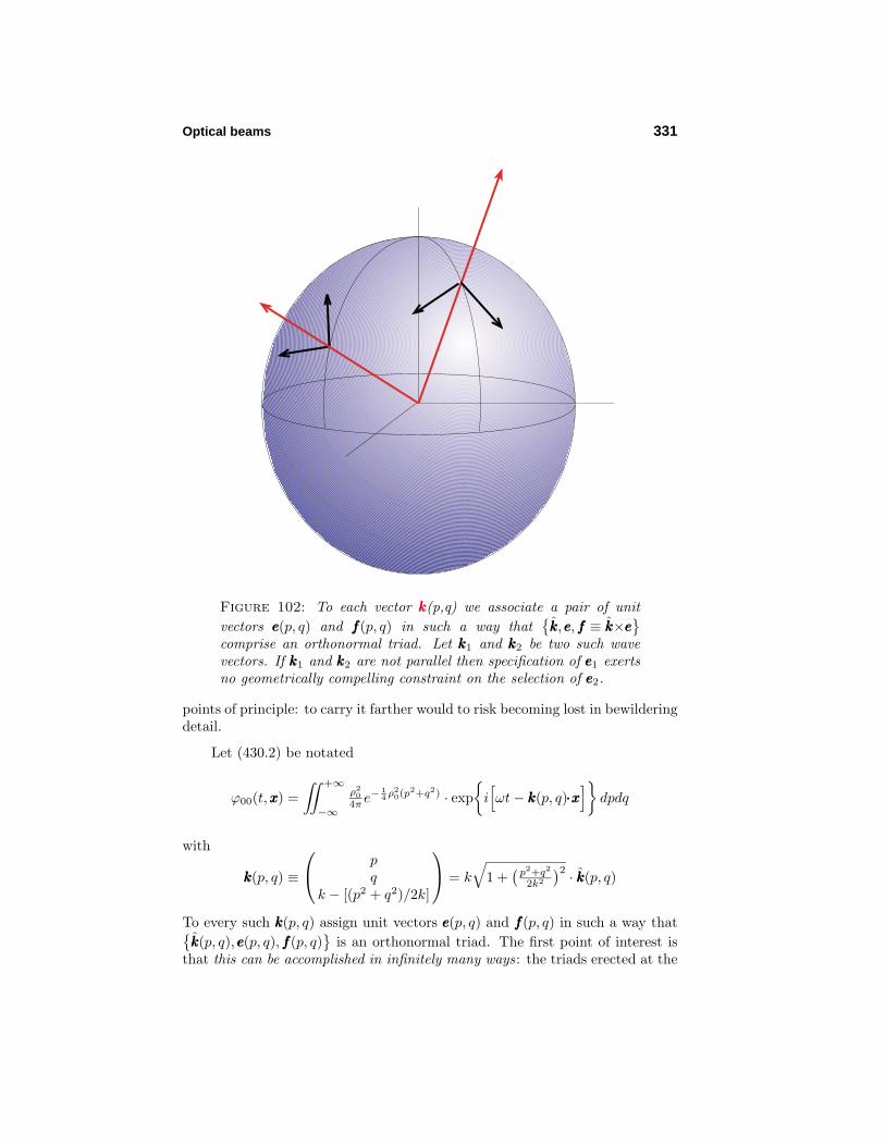
Figure 102: To each vector kkk(p,q) we associate a pair of unitvectors eee(p, q) and fff(p, q) in such a way that

kkk, eee, fff ≡ kkk×eee

comprise an orthonormal triad. Let kkk1 and kkk2 be two such wavevectors. If kkk1 and kkk2 are not parallel then specification of eee1 exertsno geometrically compelling constraint on the selection of eee2.

points of principle: to carry it farther would to risk becoming lost in bewilderingdetail.

Let (430.2) be notated

ϕ00(t, xxx) =∫∫ +∞

−∞

ρ20

4π e− 1

4 ρ20(p

2+q2) · expi[ωt− kkk(p, q)···xxx

]dpdq

with

kkk(p, q) ≡

p

qk − [(p2 + q2)/2k]

= k

√1 +

(p2+q2

2k2

)2 · kkk(p, q)

To every such kkk(p, q) assign unit vectors eee(p, q) and fff(p, q) in such a way thatkkk(p, q), eee(p, q), fff(p, q)

is an orthonormal triad. The first point of interest is

that this can be accomplished in infinitely many ways: the triads erected at the

332 Light in vacuum

points of (p, q)-space are independent creations (see Figure 102). Given suchan assignment, form

EEE(t, xxx) =∫∫ +∞

−∞

ρ20

4π e− 1

4 ρ20(p

2+q2) · EEE(p, q) expi[ωt− kkk(p, q)···xxx

]dpdq (431)

withEEE(p, q) ≡ E1(p, q)eee(p, q) + E2(p, q)eiδ(p,q)fff(p, q)

where further arbitrariness enters into the design of the functions E1(p, q),E2(p, q) and δ(p, q). The constructions

EEEp,q(t, xxx) =E1(p, q)eee(p, q) + E2(p, q)eiδ(p,q)fff(p, q)

exp

i[ωt− kkk(p, q)···xxx

]BBBp,q(t, xxx) = kkk(p, q)×EEEp,q(t, xxx)

=E1(p, q)fff(p, q) − E2(p, q)eiδ(p,q)eee(p, q)

exp

i[ωt− kkk(p, q)···xxx

]

serve—in the approximation (p2 + q2)/2k ≈ 0—to associate a monochromaticpolarized electromagnetic plane wave (propagating in the direction kkk(p, q)) witheach point of (p, q)-space, and (431) describes a Gauss-weighted superpositionof such plane waves. The “bewildering detail” to which I have referred arises(even in the simplest of the cases I have studied) when one undertakes to dothe integration.

“Electromagnetic Gaussian beams”exist, by this account, in infinite variety.Evidently one must look to the finer particulars of laser design to discover howthe physical device “selects among options,” how to construct acceptable modelsof the laser beams encountered in laboratories.

The fields

EEE(t, xxx) =∫∫ +∞

−∞

ρ20

4π e− 1

4 ρ20(p

2+q2) ·EEEp,q(t, xxx) dpdq

BBB(t, xxx) =∫∫ +∞

−∞

ρ20

4π e− 1

4 ρ20(p

2+q2) ·BBBp,q(t, xxx) dpdq

possess a property worthy of notice which I will expose by considering thesuperposition of only two electromagnetic plane waves. Let

EEE1(t, xxx) = EEE1 expi(ωt− kkk1···xxx)

: EEE1 ⊥ kkk1

BBB1(t, xxx) = kkk1×EEE1 expi(ωt− kkk1···xxx)

describe one monochromatic plane wave, and

EEE2(t, xxx) = EEE2 expi(ωt− kkk2···xxx + δ)

: EEE2 ⊥ kkk2

BBB2(t, xxx) = kkk2×EEE2 expi(ωt− kkk2···xxx + δ)

Optical beams 333

describe another. Let EEE = EEE1 +EEE2 and BBB = BBB1 +BBB2. Then

EEE ···BBB =EEE1 ···(kkk2×EEE2) + EEE2 ···(kkk1×EEE1)

︸︷︷︸ expi(2ωt− [kkk1 + kkk2]···xxx + δ)

|= (kkk1 − kkk2)···(EEE1×EEE2)= 000 except under obvious special conditions

shows that, in general, superimposed plane waves do not share the EEE ⊥ BBBcondition characteristic of individual plane waves. In particular: EEE ⊥ BBB willnot be found in the superpositions that produce “beams.”

Let us look to a concrete example. Working from

kkk(p, q) ≡ k–1

p

qk − [(p2 + q2)/2k]

in the approximation

(p2+q2

2k2

)2 ≈ 0

we complete the dimensionless orthonormal triad by writing

eee(p, q) ≡ 1√p2+q2

+q

−p0

fff(p, q) ≡ 1

2k2√

p2+q2

p[2k2 − (p2 + q2)]

q[2k2 − (p2 + q2)]−2k(p2 + q2)

= kkk(p, q)×eee(p, q)

and to achieve tractable integrals set

E1(p, q) = E1+ ·√p2 + q2

E2(p, q) = E2+ ·√p2 + q2

δ(p, q) = constant

Here + (introduced to cancel the physical dimension of√

p2 + q2 ) is a constantof arbitrary value and the dimensionality of length, so E1+ and E2+ have thedimensionality of electric potential. Working from (431) with k = 2Z/ρ2

0 and

EEE(p, q) = E1+

+q

−p0

+ E2+e

iδ

p[1 − (p2 + q2)/2k2]

q[1 − (p2 + q2)/2k2]− (p2 + q2)/k

BBB(p, q) = E1+

p[1 − (p2 + q2)/2k2]

q[1 − (p2 + q2)/2k2]− (p2 + q2)/k

− E2+e

iδ

+q

−p0

we entrust the∫∫

’s to Mathematica, who supplies

EEE(t, xxx) = E1+ eee(t, xxx) + E2+eiδ fff(t, xxx)

BBB(t, xxx) = E1+ fff(t, xxx) − E2+eiδ eee(t, xxx)

(432)

334 Light in vacuum

with

eee(t, xxx) = eG·

−Ay

+Ax0

fff(t, xxx) = eG·

−Bx

−ByC

(433)

where

eG ≡ exp− x2+y2

ρ2 [1 + i(z/Z)] + i[ωt− kz]

is familiar already (see again page 323) from the scalar theory of Gaussianbeams, and where

A = 2iZ2

ρ20(Z−iz)2

≡ Aeiα with A =√

02+2Z22

ρ40(Z

2+z2)2

B = −2Zρ20(z+iZ)+iZ2[r2−2(z+iZ)2]

ρ20(z+iZ)4

≡ Beiβ with B =√

stuff2+more stuff2

ρ40(Z

2+z2)4

C = 2Z2r2−2ρ20Z(Z−iz)

ρ20(Z−iz)3

≡ Ceiγ with C =√

stuff2+more stuff2

ρ40(Z

2+z2)3

I have indicated how the invariable reality of A, B and C comes about, buthave omitted details too complicated to be informative, and have also omitted(as irrelevant to the purposes at hand) explicit description of the phase factorsα, β and γ (which could be expressed as the arctangents of the obvious ratios).Notice that the functions described above depend upon x and y only throughr2 ≡ x2 + y2; they are, in short, axially symmetric. Notice also that[A ] = [B ] = (length)−2 while [C ] = (length)−1.

Returning now with (433) to (432), we have EEE(t, xxx) = EEE1(t, xxx) +EEE2(t, xxx)with

EEE1 = E1+e−(r/ρ)2· ei(ωt−kz)−(r/ρ)2(z/Z)

Aeiα

−y

+x0

EEE2 = E2eiδ+e−(r/ρ)2· ei(ωt−kz)−(r/ρ)2(z/Z)

Beiβ

−x

−y0

+ Ceiγ

0

01

Optical beams 335

The associated magnetic fields are

BBB1 = E1+e−(r/ρ)2· ei(ωt−kz)−(r/ρ)2(z/Z)

Beiβ

−x

−y0

+ Ceiγ

0

01

BBB2 = E2eiδ+e−(r/ρ)2· ei(ωt−kz)−(r/ρ)2(z/Z)

−Aeiα

−y

+x0

It is understood that to extract the physical fields, and before we assemble suchquadratic constructions as (field)···(field) and (field)×(field), we must make thereplacements

ei(stuff) −→ cos(stuff)

That done, we obtain finally

EEE1 = E1+e−(r/ρ)2

A cos(ϑ + α)

−y

+x0

EEE2 = E2+e−(r/ρ)2

B cos(ϑ + β + δ)

−x

−y0

+ C cos(ϑ + γ + δ)

0

01

BBB1 = E1+e−(r/ρ)2

B cos(ϑ + β)

−x

−y0

+ C cos(ϑ + γ)

0

01

BBB2 = E2+e−(r/ρ)2

−A cos(ϑ + α + δ)

−y

+x0

with ϑ ≡ ωt − kz − (r/ρ)2(z/Z). It is immediately evident that at everyspacetime point

EEE1 ⊥ EEE2 , BBB1 ⊥ BBB2

EEE1 ⊥ BBB1 , EEE2 ⊥ BBB2

but from

EEE ···BBB = (EEE1 +EEE2)···(BBB1 +BBB2)

= E1E2+2e−2(r/ρ)2

r2

[B2 cos(ϑ+β) cos(ϑ+β+δ)

−A2 cos(ϑ+α) cos(ϑ+α+δ)]

+C2 cos(ϑ+γ) cos(ϑ+γ +δ)

= 0 except under non-obvious special conditions: note, however, that↓= 0 as r → ∞ because the fields die at points far from the beam axis

we see that—consistently with the remark developed on page 332—the net fieldsEEE and BBB are typically not perpendicular: at axial points (r = 0) they are, in

336 Light in vacuum

fact, parallel ! The energy flux and momentum density at the spacetime pointare proportional to

EEE×BBB = (EEE1 +EEE2)×(BBB1 +BBB2) ≡ e−2(r/ρ)2 · FFF

where according to Mathematica

F1 = xAC[E2

1 cos(ϑ + α) cos(ϑ + γ) + E22 cos(ϑ + α + δ) cos(ϑ + γ + δ)

]− yBCE1E2

[cos(ϑ + β + δ) cos(ϑ + γ) − cos(ϑ + β) cos(ϑ + γ + δ)

]F2 = yAC

[E2

1 cos(ϑ + α) cos(ϑ + γ) + E22 cos(ϑ + α + δ) cos(ϑ + γ + δ)

]+ xBCE1E2

[cos(ϑ + β + δ) cos(ϑ + γ) − cos(ϑ + β) cos(ϑ + γ + δ)

]F3 = r2AB

[E2

1 cos(ϑ + α) cos(ϑ + β) + E22 cos(ϑ + α + δ) cos(ϑ + β + δ)

]This is of the design

FFF = a

x

y0

+ b

−y

+x0

+ c

0

01

= FFF radial + FFF tangential + FFF axial

where the vectors FFF radial stand normal to the z-axis (beam-axis) and are ofconstant magnitude on circles concentric about that axis, the vectors FFF tangential

are (also constant on but) tangent to such circles and have or handednessaccording as b ≷ 0, and the vectors FFF axial (also constant on such circles) runparallel to the z-axis. The “constants” a, b and c are in fact horribly complicatedfunctions of the variables

t, z, r

and of the parameters

ω, ρ0, Z,E1,E2, δ

.

We are in position now to state that the momentary momentum density ofthe beam field at any designated point xxx can be described (see again page 216)

PPP = 1ce

−2(r/ρ)2FFF

We observe that• PPP vanishes far from the beam axis because of Gaussian attenuation• PPP vanishes on the beam axis by the design of a, b and c

• field momentum traces a divergent spiral in the near neighborhood of thebeam axis unless b = 0.

The angular momentum density of the beam field is given by262

LLL = xxx×PPP = 1ce

−2(r/ρ)2

−bz

x

y0

+ (az − c)

−y

+x0

+ br2

0

01

= LLLradial + LLLtangential + LLLaxial

262 Don’t be confused by the fact that c is used here to mean two entirelydifferent things.

Optical beams 337

Figures 103 & 104: The upper figure portrays the spiroformdeployment of the momentum in the electromagnetic field of theGaussian beam described in the text. Displayed below is the resultingangular momentum density (presented as a function of x and y atthe beam waist: z = 0). The figures show that/why it makes sense tosay that “the angular momentum lives at the fringes of the beam.”

338 Light in vacuum

The first two components (by an elementary symmetry argument) can make nonet contribution to the total angular momentum of the beam, which is giventherefore by

LLL = L

0

01

with L =

∫∫∫1ce

−2(r/ρ)2br2 dxdydz

We notice that L vanishes if b = 0, and that this happens when δ = 0, for inthe latter circumstance the equations at near the top of page 336 assume themuch-simplified form

F1 = xAC[E2

1 + E22

]cos(ϑ + α) cos(ϑ + γ) + no y-term

F2 = yAC[E2

1 + E22

]cos(ϑ + α) cos(ϑ + γ) + no x-term

F3 = r2AB[E2

1 + E22

]cos(ϑ + α) cos(ϑ + β)

One occasionally encounters the claim that “the angular momentumtransported by a laser beam lives at the fringes of the beam,” but in supportof that claim authors who possess only a scalar theory of beams must arguerather vaguely that

i) beam angular momentum must arise from momentum circulationii) there can be no circulation at the axis of an axially-symmetric beamiii) all PPP-circulation must therefore occur between the axis and the remote

regions where the EEE and BBB fields have fallen off to zero—in short: “at thefringes” of the beam.

My effort has been to carry a vector theory of beams far enough to illuminatethe details of the matter. Having achieved that objective, I must be contentnow to abandon my little “electromagnetic theory of beams”. . . but feel anobligation to list some of the respects in which the theory remains incomplete:

• It should be feasible (by the method sketched on page 321) to turn suchbeams on and off; i.e., to construct laterally confined quasi-monochromaticGaussian wavepackets—“classical photons,” if you will.

• It should be feasible, moreover, to construct trains of such wavepackets,and to describe the coherence/polarization properties of such trains.

• One would like to be in position to describe the energy, momentum andangular momentum transported by such a “classical photon,” and toidentify conditions under which they stand in the quantum relationships

E = cP = ωL

• To that end one would need to clarify certain salient properties of andinterrelationships among the complicated functions a, b and c.

• Identical values of E1, E2 and δ were assigned to each of the plane wavesfrom which ourGaussian beams were assembled. Do the Stokes parametersimplicit (by (399)) in

E1,E2, δ

speak usefully about the polarization

properties of the assembled beam?

Optical beams 339

It should be borne always in mind that the theory sketched above proceedsfrom an inoffensive approximation (page 322) and—within the bounds of thatapproximation—from a convenient specification (page 333) of the manner inwhich orthonormal vectors will be attached to kkk -vectors (and weighted). Thetheory is rich enough to support easily the notion of “higher beam modes,” butthis question remains open: Is the theory—as I suspect—rich enough to accountfor the observed properties of the optical beams encountered in laboratories?

light in vacuum - reed college

Documents