Lifelong Localization in Changing Environments

Gian Diego Tipaldi∗ Daniel Meyer-Delius† Wolfram Burgard∗∗Department of Computer Science, University of Freiburg, D-79110 Freiburg, Germany.

†KUKA Laboratories GmbH, D-86165 Augsburg, Germany.

Abstract—Robot localization systems typically assume that theenvironment is static, ignoring the dynamics inherent in mostreal-world settings. Corresponding scenarios include households,offices, warehouses and parking lots, where the location ofcertain objects such as goods, furniture or cars can change overtime. These changes typically lead to inconsistent observationswith respect to previously learned maps and thus decrease thelocalization accuracy or even prevent the robot from globallylocalizing itself. In this paper we present a sound probabilisticapproach to lifelong localization in changing environments usinga combination of a Rao-Blackwellized particle filter with a hiddenMarkov model. By exploiting several properties of this model, weobtain a highly efficient map management approach for dynamicenvironments, which makes it feasible to run our algorithmonline. Extensive experiments with a real robot in a dynamicallychanging environment demonstrate that our algorithm reliablyadapts to changes in the environment and also outperforms thepopular Monte-Carlo localization approach.

I. INTRODUCTION

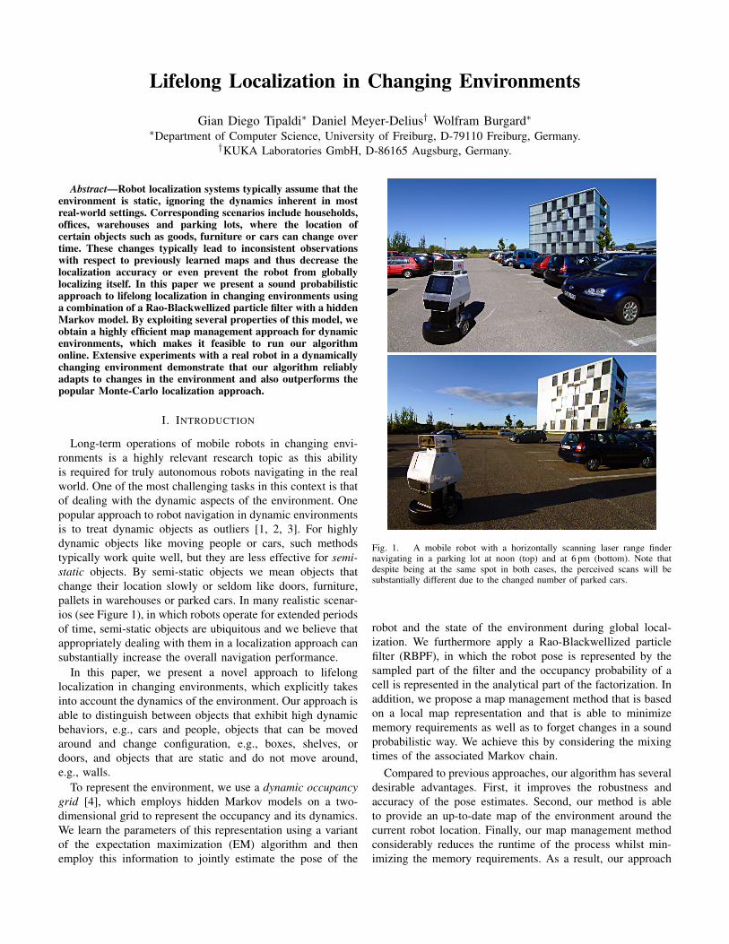
Long-term operations of mobile robots in changing envi-ronments is a highly relevant research topic as this abilityis required for truly autonomous robots navigating in the realworld. One of the most challenging tasks in this context is thatof dealing with the dynamic aspects of the environment. Onepopular approach to robot navigation in dynamic environmentsis to treat dynamic objects as outliers [1, 2, 3]. For highlydynamic objects like moving people or cars, such methodstypically work quite well, but they are less effective for semi-static objects. By semi-static objects we mean objects thatchange their location slowly or seldom like doors, furniture,pallets in warehouses or parked cars. In many realistic scenar-ios (see Figure 1), in which robots operate for extended periodsof time, semi-static objects are ubiquitous and we believe thatappropriately dealing with them in a localization approach cansubstantially increase the overall navigation performance.

In this paper, we present a novel approach to lifelonglocalization in changing environments, which explicitly takesinto account the dynamics of the environment. Our approach isable to distinguish between objects that exhibit high dynamicbehaviors, e.g., cars and people, objects that can be movedaround and change configuration, e.g., boxes, shelves, ordoors, and objects that are static and do not move around,e.g., walls.

To represent the environment, we use a dynamic occupancygrid [4], which employs hidden Markov models on a two-dimensional grid to represent the occupancy and its dynamics.We learn the parameters of this representation using a variantof the expectation maximization (EM) algorithm and thenemploy this information to jointly estimate the pose of the

Fig. 1. A mobile robot with a horizontally scanning laser range findernavigating in a parking lot at noon (top) and at 6 pm (bottom). Note thatdespite being at the same spot in both cases, the perceived scans will besubstantially different due to the changed number of parked cars.

robot and the state of the environment during global local-ization. We furthermore apply a Rao-Blackwellized particlefilter (RBPF), in which the robot pose is represented by thesampled part of the filter and the occupancy probability of acell is represented in the analytical part of the factorization. Inaddition, we propose a map management method that is basedon a local map representation and that is able to minimizememory requirements as well as to forget changes in a soundprobabilistic way. We achieve this by considering the mixingtimes of the associated Markov chain.

Compared to previous approaches, our algorithm has severaldesirable advantages. First, it improves the robustness andaccuracy of the pose estimates. Second, our method is ableto provide an up-to-date map of the environment around thecurrent robot location. Finally, our map management methodconsiderably reduces the runtime of the process whilst min-imizing the memory requirements. As a result, our approach

allows a robot to localize itself and to simultaneously estimatea local configuration of the environment in an online fashion.

This paper is organized as follows. After discussing relatedwork in Section II, we provide a more precise formulation ofthe problem in Section III. We then present an overview aboutthe dynamic occupancy grid representation in Section IV. InSection V, we explain the algorithm for the joint estimationand the map management. Finally, in Section VI, we presentextensive experiments carried out with a real robot, showingthat our approach significantly outperforms state-of-the-artlocalization methods in changing environments in terms ofthe accuracy and robustness of the localization process andthe consistency of the generated maps.

II. RELATED WORK

Localization in dynamic environments has been an activetopic in robotics research in the last decade. Many proposedapproaches treat dynamic objects as outliers and hence filterout observations of dynamic objects. The observations ofthe static part of the environment are then used to per-form map building, localization and navigation. For example,Fox et al. [1] used an entropy gain filter and a distancefilter based on the expected distance of a measurement,while Schultz et al. [2] considered local minima of rangemeasurement as observations from dynamic objects if they donot match an already available map. Montemerlo et al. [5] usedobservations of humans for people tracking while localizingthe robot. The tracking of people simplifies the rejection ofreadings due to dynamic objects and increases reliability inpopulated environments. They employed a conditional particlefilter to estimate the position of people conditioned to the poseof the robot, thus also enabling tracking in the presence ofglobal uncertainty of the robot pose.

The main limitation of those approaches, however, is thatthey rely on the static world assumption for the underlyingnavigation system. In environments that change configurationsover time or where the dynamics are low, e.g., parkinglots, warehouses, apartments and cluttered environments, thechanges may persist over long periods of time and could beuseful to localize the robot. In extreme situations, the partsof the static environments that are visible are not informativeenough for a reliable navigation and reasoning about changesis of utmost importance. In this paper we address those limi-tations and propose a localization system able to reason aboutchanges and use that information to improve the localizationperformances.

Other approaches specifically focus on separating the staticand dynamic aspects of the environment by building twomaps. Wolf and Sukhatme [6] proposed a model that maintainstwo separate occupancy grids, one for the static parts ofthe environment and the other for the dynamic parts. Wanget al. [7] formulated a general framework for mapping anddynamic object detection by employing a system to detect ifa measurement is caused by a dynamic object. Montesano etal. [8] extended the previous approach by jointly consideringthe problem of dynamic object detection with the one of

mapping and including the error estimation of the robot inthe classifier. Similarly, Gallagher et al. [9] built maps forindividual objects that can then be overlaid to represent thecurrent configuration of the environment. Hahnel et al. [3],on the other hand, combined the EM algorithm and a sensormodel that considers dynamic objects to obtain accurate maps.The approach of Anguelov et al. [10] computes shape modelsof non-stationary objects. In their approach, the authors createdmaps at different points in time and compared those mapsusing an EM-based algorithm to identify the parts of theenvironment that change over time.

Although those approaches do not simply consider observa-tions of dynamic objects as outliers, they still rely on a staticrepresentation of the environment to perform navigation. Theirmain advantage over filtering dynamic observations is that theyare able to provide a better static map of the environment andthe detection of dynamic observations can be done in a morereliable way. However, they still share the same limitationsof the static world assumptions when deployed in changingenvironments or where the dynamics are low.

In order to overcome the limitations due to the static worldassumptions, some authors worked on how to model thedynamics of the environment in a single unified representation.Chen et al. [11] and lately Brechtel et al. [12] extended theoccupancy grid paradigm to include moving objects. Theirapproach, the Bayesian occupancy filter, is based on the ideathat since occupancy is caused by objects, when those objectsmove, the corresponding occupied cell of the map shouldmove accordingly. From this point of view, They propose anobject-centered representation of the dynamics, and every cellin the environment need to be tracked over time. Moreover,the state transitions are assumed to be given a priori andno algorithm to learn them from data is presented. On thecontrary, we follow a map-centric approach and model howthe environment changes in an agnostic way with respect tothe cause of the change.

Biber and Duckett [13] proposed a model that represents theenvironment on multiple timescales simultaneously. For eachtimescale a separate sample-based representation is maintainedand updated using the observations of the robot according toan associated timescale parameter. Our approach differs fromtheirs in the sense that we fuse all the different maps into aunified representation and provide tools to estimate the optimaltimescale parameter for each cell. Moreover their approach hashigher memory and computational requirements than ours. Inglobal localization settings, multiple hypotheses over the stateof the environment are needed, thus memory requirements arean important aspect to be considered.

Yang and Wang [14] proposed the feasibility grids to facili-tate the representation of both the static scene and the movingobjects. A dual sensor model is used to discriminate betweenstationary and moving objects in mobile robot localization.Their work, however, assumes that the position of the robot isknown with a certain accuracy to compute and update the mapsand therefore is not suited to be used for global localizationproblems.

Recently, Saarinen et al. [15] proposed to model the en-vironment as a set of independent Markov chains, one pergrid cell, each with two states. The state transition parametersare learned on-line and modeled as two Poisson processes.A strategy based on recency weighting is used to deal withnon-stationary cell dynamics. Their representation is verysimilar to the one used in our paper but differs from the waythe occupancy probabilities are computed and the transitionslearned. The focus of the presented work, however, is to showthat Markov chain based representations can be effectivelyused for localization. Both representation could be used andwe believe would produce similar results.

Some other works have been introduced in the past withthe aim to address global localization problems in dynamicenvironments. However, to the best of our knowledge, noneof them is general enough to work with different dynamicsand objects or in real-world scenarios. Murphy et al. [16]proposed to apply a Rao-Blackwellized particle filter solutionto the SLAM problem and showed that it could also deal withdynamic maps in a theoretical way. Their approach, however,assumes that the probabilities of changing state is independentfrom the current state of the environment and is given apriori. Moreover, they only presented results in small scaleenvironments and with known initial position. In this paper weextend their representation and show how it can be used forglobal localization introducing a novel memory managementstrategy.

To handle the complexity of the Rao-Blackwellized particlefilter solution in practical applications, some authors proposeto focus on only some dynamic aspects or restrict the dynamicsto a set of static configurations. Avots et al. [17], used the Rao-Blackwellized particle filter to estimate the pose of the robotand the state of doors in the environment. They representedthe environment using a reference occupancy grid where thelocation of the doors is known, but not their state (i.e.,opened or closed). Petrovskaya and Ng [18] proposed a similarapproach where instead of a binary model, a parametrizedmodel (i.e., opening angle) of the doors is used. Stachnissand Burgard [19] clustered local grid maps to identify aset of possible configurations of the environment. The Rao-Blackwellized particle filter is then used to localize the robotand estimate the configuration of the environment from theset. In contrast to their methods, we estimate the state of thecomplete environment, and not only of a small, specific areaor element. Additionally, we also learn the model parametersfrom data and we are able to generalize over unforeseenenvironment configurations.

Meyer-Delius et al. [20] kept track of the observationscaused by unexpected objects in the environment using tem-porary local maps. The robot pose is then estimated usinga particle filter that relies both on these temporary localmaps and on a reference map of the environment. The work,however, still relies on a static map for global localization andtemporary maps are only created when a failure in positiontracking occurs.

An interesting approach to lifelong mapping in dynamic

environments has been presented by Konolige et al. [21].The approach focuses mainly on visual maps, and presents aframework where local maps (views) can be updated over timeand new local maps are added/deleted when the configurationof the environment changes. Using similar ideas, Kretzschmaret al. [22], applied graph compression using an efficientinformation-theoretic graph pruning strategy. The approachcan be used with a bias on more recent observations to obtain asimilar behavior of the work of Konolige et al. [21]. Those twoapproaches, however, mainly focus on the scalability problemsarising in long-term operations and not on the dynamicalaspect of environments changing over time.

The approach of Walcott-Bryant et al. [23] follows a similaridea as well. They introduce a novel representation, the Dy-namic Pose Graph (DPG), to perform SLAM in environmentswith low dynamics over long periods of time. Their approach,DPG-SLAM, assumes that data association is solved usingscan matching and that the starting position of the robot isknown and coincides with the last pose of the previous run.On the contrary, our approach can deal with different dynamics(low, medium and high) and does not require the knowledgeof the initial position of the robot.

Churchill and Newman [24] presented a different point ofview to the problem of lifelong mapping. They reason thata global reference frame is not needed in navigation andintroduce experiences, i.e., robot paths with relative metricalinformation. Experiences can be connected together usingappearance-based data association methods and places thatchange over time are represented by a set of different ex-periences.

Their work is similar in spirit and generalizes both Stachnissand Burgard [19] and Meyer-Delius et al. [20]. In our paperwe take another perspective, where we propose a model-basedapproach in contrast to the data-driven one of Churchill andNewman [24]. We believe that having a unified model ofthe environments is important for human robot interaction.Navigation tasks, e.g., go to a specific position or follow aspecific path, only need to be defined once in model-basedapproaches. Using the experience approach, on the contrary,requires the user to define the same task on every experi-ence the robot recorded. This may increase the complexityof human-robot interaction and reduce the reliability of thesystem, since maintaining the task consistence across differentexperiences is not trivial. Moreover, with our approach, we arealso able to predict how part of the environment will look inthe future, by directly modeling their rate of change.

III. PROBLEM STATEMENT

Imagine a robot that continuously performs tasks during asession, i.e., until its battery runs out. It then gets back to itscharging station and, when charged, continues to perform theprevious tasks in the next session. To perform its tasks, therobot knows the positions of several locations of interest andplans paths to reach them avoiding obstacles. These locationsneed to be consistent between several sessions, to reduce theteaching effort of the user. One way to ensure this is to use a

single map and express those locations in a global referenceframe. Localizing the robot in the global frame allows thento know the displacement between the current robot pose andthe locations of interest.

In static environments, the map does not change betweendifferent sessions. This simplifies the problem and a readilyavailable solution is to build a map of the environment duringthe first session using a SLAM algorithm [25] and then usethe computed map for localization in the remaining sessions.This solution is very mature, effective, and robust to minorchanges in the environment and dynamic objects [26]. Never-theless, if the amount of changes increases and low dynamicphenomena appear (i.e., boxes that stay for long, parked cars,moved furniture, etc . . . ) such a solution loses reliability andprecision. The robot starts to get de-localized and invalid pathsare planned, since the map does not represent the current stateof the environment.

In those cases, since the environment changes over timeand the map needs to be updated, a straightforward solutionwould be to always use a SLAM algorithm and rely onloop closure techniques to join the trajectories of subsequentsessions together. This approach has several shortcomings,which we will show in more details in Section VI. A firstproblem consists in scalability issues. In case a graph-basedapproach for SLAM is used, the amount of data that needsto be processed grows linearly with the length of the traveledpath. Data compression techniques have been developed todiscard measurements according to the entropy of the mapdistribution or some decay value. Those techniques representa step towards the solution although the more general explo-ration vs. exploitation aspect – when to stop mapping andstart localizing – still remains. Filtering based approaches forSLAM may be better fitted in this case, since the trajectoriesare marginalized out and their complexity scales with the sizeof the environment. However, filtering approaches do not scalewell with respect to the size of the environment and do notoffer the flexibility of graph-based approaches to select whichobservations to use at the moment to have an up-to-date map.

A second problem regards data association issues. Algo-rithms designed for static environments may fail in dynamicones since unexplained measurements can be caused by eitherincorrect localization or environment changes. Optimizationsolutions to SLAM cannot be used effectively, since a singlehypothesis is not sufficient to disambiguate those situations.Moreover, no assumption can be made on the prior location ofthe robot between multiple sessions of the lifelong operation,since the robot starting position may have been changed aswell. One way of addressing this point is to use multiple-hypotheses filters for SLAM, where each hypothesis carriesits own map. In the case of medium-sized environments andunknown initial location, this leads to high memory consump-tion and scalability issues. Finally, static representations of theenvironment are not suited for lifelong navigation in changingenvironments. The reason is that they are slow to be updatedwhen a change happens, since they have a memory effectand they need to observe an occupied cell as free as many

times as it was observed as occupied to change its state. Anexperimental evaluation of these shortcomings with additionalinsights is presented in Section VI.

In this paper, we aim at presenting another point of viewfor the lifelong localization problem. We argue that addressingit as a pure SLAM or localization problem is suboptimaland that is because this problem is neither an instance of aSLAM problem nor of a pure localization problem. It is, in ouropinion, a hybrid problem that lies in-between them and needsto be tackled in a particular way. In the remainder of the paper,we will describe our solution to the problem by first describinga map representation tailored for dynamic environments andthen an efficient and effective algorithm to jointly estimate thepose of the robot and the environment configuration.

IV. OCCUPANCY GRIDS FOR CHANGING ENVIRONMENTS

Occupancy grids [27] are one of the most popular repre-sentations of a mobile robot’s environment. They partitionthe space into rectangular cells and store, for each cell, aprobability value indicating whether the underlying area ofthe environment is occupied by an obstacle or not.

One of the main disadvantages of occupancy grids for ourproblem is that they assume the environment to be static. Tobe able to deal with changes in the environment we utilize adynamic occupancy grid [4], a generalization of an occupancygrid that overcomes the static-world assumption by explicitlyaccounting for changes in the environment. In the remainderof this section, we give a short overview on the representationand in the next section we will describe how it can be usedfor global localization.

The map consists of a collection of individual cells, mt =

{c(i)t }, where each cell is modeled using an hidden Markovmodel (HMM) and requires the specification of a state tran-sition probability, an observation model, and an initial statedistribution. We adopt the same assumptions of the occupancygrid model, namely the independence of the individual ob-servations, given the map, and the independence among thecells. Those assumptions are needed for having an efficientinference during localization. We believe those are reasonableassumptions and, during our experiments, we did not observeany critical issues either in localization or in the accuracy ofthe map.

Let ct be a discrete random variable that represents the oc-cupancy state of a cell c at time t. The initial state distributionp(c0) specifies the occupancy probability of a cell at the initialtime step t = 0 prior to any observation.

The state transition model p(ct | ct−1) describes the evolu-tion of the cell between consecutive time steps. In their paper,the authors assume that changes in the environment are causedby a stationary process, that is, the state transition probabilitiesare the same for all time steps t. Since a cell is either free (free)or occupied (occ), the state transition model can be specifiedusing only two transition probabilities, namely

po|fc = p(ct = occ | ct−1 = free) (1)

andpf |oc = p(ct = free | ct−1 = occ) . (2)

Note that, by assuming a stationary process, these probabilitiesdo not depend on the absolute value of t. Therefore, thedynamics of a cell at any time can be captured by its transitionmatrix

Ac =

[1− pf |oc p

f |oc

po|fc 1− po|fc

]. (3)

This transition model generalizes the one utilized by Mur-phy et al. [16] and Chen et al. [11] where po|fc = p

f |oc .

The observation model p(z | c) represents the likelihood ofthe observation z given the state of the cell c. In our case, itcorresponds to the sensor model of a laser range finder. Giventhe limited field of view of the sensor, we additionally considerthe case where no direct measurement is observed by thesensor. Explicitly considering this no-observation case allowsus to update and estimate the parameters of the model usingthe HMM framework directly without having to artificiallydistinguish between cells that are observed and cells that arenot. The probabilities can be specified by three matrices

Bz =

[p(z | c = occ) 0

0 p(z | c = free)

], (4)

where z ∈ {hit,miss, no-observation}.The update of the occupancy state of the cells follows

a Bayesian approach. The goal is to estimate the posteriordistribution p(ct | z1:t) over the current occupancy state ct ofa cell given all the available evidence z1:t up to time t. Theupdate formula is:

p(ct | z1:t) =

η p(zt | ct)∑ct−1

p(ct | ct−1) p(ct−1 | z1:t−1) , (5)

where η is a normalization constant. The structure of HMMsallows for a simple and efficient implementation of thisrecursive approach. Utilizing the matrix notation and definingthe posterior at time t as the vector

Qt =[p(ct = occ | z1:t) p(ct = free | z1:t)

], (6)

one can compute the posterior at time t+ 1 as

Qt+1 = QtAcBzt+1η . (7)

Note that the map update for occupancy grids is a specialcase of our update equations, where the sum in (5) is replacedwith the posterior p(ct | z1:t−1), or equivalently, the matrixAc in (7) is replaced with the identity matrix I .

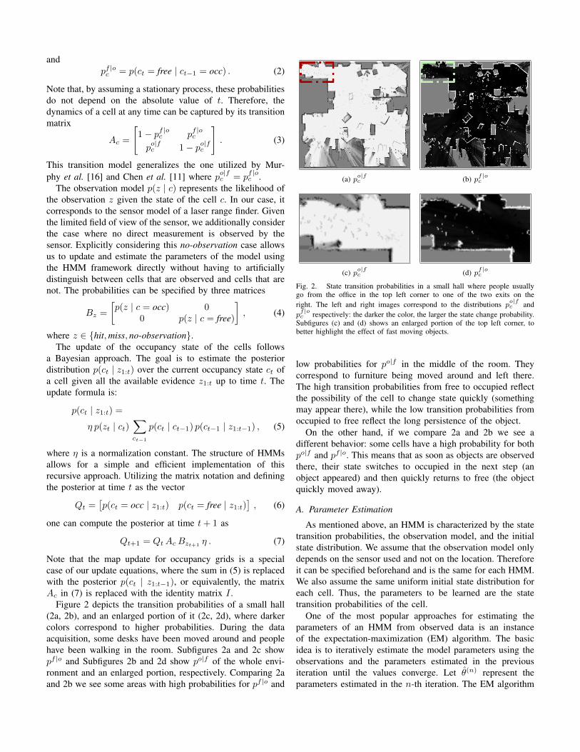
Figure 2 depicts the transition probabilities of a small hall(2a, 2b), and an enlarged portion of it (2c, 2d), where darkercolors correspond to higher probabilities. During the dataacquisition, some desks have been moved around and peoplehave been walking in the room. Subfigures 2a and 2c showpf |o and Subfigures 2b and 2d show po|f of the whole envi-ronment and an enlarged portion, respectively. Comparing 2aand 2b we see some areas with high probabilities for pf |o and

(a) po|fc (b) pf |oc

(c) po|fc (d) pf |oc

Fig. 2. State transition probabilities in a small hall where people usuallygo from the office in the top left corner to one of the two exits on theright. The left and right images correspond to the distributions po|fc andpf |oc respectively: the darker the color, the larger the state change probability.

Subfigures (c) and (d) shows an enlarged portion of the top left corner, tobetter highlight the effect of fast moving objects.

low probabilities for po|f in the middle of the room. Theycorrespond to furniture being moved around and left there.The high transition probabilities from free to occupied reflectthe possibility of the cell to change state quickly (somethingmay appear there), while the low transition probabilities fromoccupied to free reflect the long persistence of the object.

On the other hand, if we compare 2a and 2b we see adifferent behavior: some cells have a high probability for bothpo|f and pf |o. This means that as soon as objects are observedthere, their state switches to occupied in the next step (anobject appeared) and then quickly returns to free (the objectquickly moved away).

A. Parameter Estimation

As mentioned above, an HMM is characterized by the statetransition probabilities, the observation model, and the initialstate distribution. We assume that the observation model onlydepends on the sensor used and not on the location. Thereforeit can be specified beforehand and is the same for each HMM.We also assume the same uniform initial state distribution foreach cell. Thus, the parameters to be learned are the statetransition probabilities of the cell.

One of the most popular approaches for estimating theparameters of an HMM from observed data is an instanceof the expectation-maximization (EM) algorithm. The basicidea is to iteratively estimate the model parameters using theobservations and the parameters estimated in the previousiteration until the values converge. Let θ(n) represent theparameters estimated in the n-th iteration. The EM algorithm

...

...

...

...

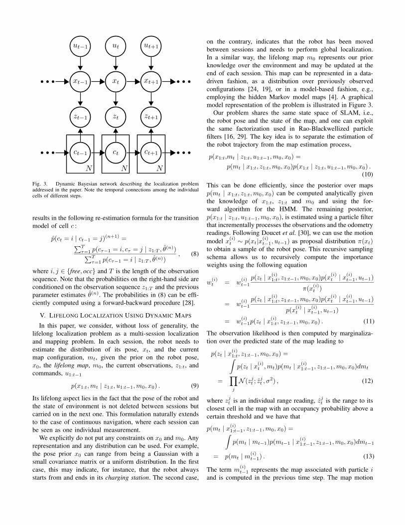
Fig. 3. Dynamic Bayesian network describing the localization problemaddressed in the paper. Note the temporal connections among the individualcells of different steps.

results in the following re-estimation formula for the transitionmodel of cell c :

p(ct = i | ct−1 = j)(n+1) =∑Tτ=1 p(cτ−1 = i, cτ = j | z1:T , θ(n))∑T

τ=1 p(cτ−1 = i | z1:T , θ(n)), (8)

where i, j ∈ {free, occ} and T is the length of the observationsequence. Note that the probabilities on the right-hand side areconditioned on the observation sequence z1:T and the previousparameter estimates θ(n). The probabilities in (8) can be effi-ciently computed using a forward-backward procedure [28].

V. LIFELONG LOCALIZATION USING DYNAMIC MAPS

In this paper, we consider, without loss of generality, thelifelong localization problem as a multi-session localizationand mapping problem. In each session, the robot needs toestimate the distribution of its pose, xt, and the currentmap configuration, mt, given the prior on the robot pose,x0, the lifelong map, m0, the current observations, z1:t, andcommands, u1:t−1

p(x1:t,mt | z1:t, u1:t−1,m0, x0) . (9)

Its lifelong aspect lies in the fact that the pose of the robot andthe state of environment is not deleted between sessions butcarried on in the next one. This formulation naturally extendsto the case of continuous navigation, where each session canbe seen as one individual measurement.

We explicitly do not put any constraints on x0 and m0. Anyrepresentation and any distribution can be used. For example,the pose prior x0 can range from being a Gaussian with asmall covariance matrix or a uniform distribution. In the firstcase, this may indicate, for instance, that the robot alwaysstarts from and ends in its charging station. The second case,

on the contrary, indicates that the robot has been movedbetween sessions and needs to perform global localization.In a similar way, the lifelong map m0 represents our priorknowledge over the environment and may be updated at theend of each session. This map can be represented in a data-driven fashion, as a distribution over previously observedconfigurations [24, 19], or in a model-based fashion, e.g.,employing the hidden Markov model maps [4]. A graphicalmodel representation of the problem is illustrated in Figure 3.

Our problem shares the same state space of SLAM, i.e.,the robot pose and the state of the map, and one can exploitthe same factorization used in Rao-Blackwellized particlefilters [16, 29]. The key idea is to separate the estimation ofthe robot trajectory from the map estimation process,

p(x1:t,mt | z1:t, u1:t−1,m0, x0) =

p(mt | x1:t, z1:t,m0, x0)p(x1:t | z1:t, u1:t−1,m0, x0) .(10)

This can be done efficiently, since the posterior over mapsp(mt | x1:t, z1:t,m0, x0) can be computed analytically giventhe knowledge of x1:t, z1:t and m0 and using the for-ward algorithm for the HMM. The remaining posterior,p(x1:t | z1:t, u1:t−1,m0, x0), is estimated using a particle filterthat incrementally processes the observations and the odometryreadings. Following Doucet et al. [30], we can use the motionmodel x(i)t ∼ p(xt|x(i)t−1, ut−1) as proposal distribution π(xt)to obtain a sample of the robot pose. This recursive samplingschema allows us to recursively compute the importanceweights using the following equation

w(i)t = w

(i)t−1

p(zt | x(i)1:t, z1:t−1,m0, x0)p(x(i)t | x

(i)t−1, ut−1)

π(x(i)t )

= w(i)t−1

p(zt | x(i)1:t, z1:t−1,m0, x0)p(x(i)t | x

(i)t−1, ut−1)

p(x(i)t | x

(i)t−1, ut−1)

= w(i)t−1p(zt | x

(i)1:t, z1:t−1,m0, x0) . (11)

The observation likelihood is then computed by marginaliza-tion over the predicted state of the map leading to

p(zt | x(i)1:t, z1:t−1,m0, x0) =∫p(zt | x(i)t ,mt)p(mt | x(i)1:t−1, z1:t−1,m0, x0)dmt

=∏j

N (zjt ; zjt , σ

2) , (12)

where zjt is an individual range reading, zjt is the range to itsclosest cell in the map with an occupancy probability above acertain threshold and we have that

p(mt | x(i)1:t−1, z1:t−1,m0, x0) =∫p(mt | mt−1)p(mt−1 | x(i)1:t−1, z1:t−1,m0, x0)dmt−1

= p(mt | m(i)t−1) . (13)

The term m(i)t−1 represents the map associated with particle i

and is computed in the previous time step. The map motion

Algorithm 1: RBPF-HMM for Changing EnvironmentsIn: The previous sample set St−1, the lifelong map m0,

the current observation zt and odometry utOut: The new sample set St

1 St = {}2 foreach s

(i)t−1 in St−1 do

3 < x(i)1:t−1,m

(i)t−1, w

(i)t−1 >= s

(i)t−1

// State prediction

4 x(i)t ∼ p(xt|x

(i)t−1, ut−1)

5 x(i)1:t = x

(i)t ∪ x

(i)1:t−1

6 foreach ct−1 in m(i)t−1 do

7 p(ct | z1:t−1) =∑

ct−1∈{f,o}

p(ct | ct−1)p(ct−1 | z1:t−1)

8 end

// Weight computation

9 w(i)t = w

(i)t−1

∏j

N (zjt ; zjt , σ

2)

// Map update

10 foreach ct in m(i)t do

11 p(ct | z1:t) = ηp(zt | ct)p(ct | z1:t−1)12 end13 St = St ∪ {< x

(i)1:t,m

(i)t , w

(i)t >}

14 end

// Normalize the weights15 normalize(St)

// Resample

16 Neff =1∑

i(w(i)t )2

17 if Neff < T then18 St = resample(St)19 end

model p(mt | m(i)t−1) is computed using the HMM as described

in Section IV. Note that the disappearance of the integral isnot an approximation but a direct consequence of using thelikelihood field model [31] and the Dirac distribution for theparticle.

To improve the robustness against objects with high dynam-ics, we applied a robust likelihood function when computingthe weights. This approach is similar in spirit to the works inwhich high dynamic objects are treated as outliers [1, 2].

The overall process for global localization proposed in thispaper is summarized in Algorithm 1.

Note that our representation resembles the one used forSLAM and for Monte Carlo localization approaches. Thepresented problem, however, differs from them with respectto the assumptions made. In the common SLAM formulation,one assumes to have no information on the map (uniformdistribution) and to know the initial pose with certainty (Diracdistribution). In global localization, on the contrary, the map

is assumed to be static and known (Dirac distribution) and aweak prior on the initial pose is available (uniform distributionon the free space or Gaussian). Our problem is somewhat inbetween, since we assume a weak prior on the initial pose,like in global localization, and a weak prior on the map (thedynamic occupancy grid in our case).

A. Map Management

As already mentioned above, the distribution of the initialpose of the robot is generally unknown and it may be uni-formly distributed over the environment. This forces us to use ahigh number of particles, generally in thousands, to accuratelyrepresent the initial distribution. Since every particle needsto have its own estimate of the map, memory managementis a key aspect of the whole algorithm. It is worth noticingthat even if memory is becoming cheap and available in largequantity, the amount needed is still beyond what is currentlyavailable. As an example, in an environment of 200x200 m2,stored at a resolution of 0.1 m, and using 10, 000 particleswe need about 50 GB of memory. In order to save memory,we want to only store the cells in the map that have beenconsiderably changed from the lifelong map m0, which isshared among the different particles. This is done by exploitingtwo important aspects of the Markov chain associated to theHMM: the stationary distribution and the mixing time.

The occupancy value of a cell converges to a uniquestationary distribution π as the number of time steps for that noobservation is available tends to infinity [32]. This stationarydistribution represents the case where the environment hasnot been observed for a long time and is represented by thelimit distribution of our lifelong map m0. In the case of abinary HMM as the one used in this paper, this distribution iscomputed using the transition probabilities[

πf

πo

]=

1

po|fc + p

f |oc

[pf |oc

po|fc

]. (14)

Every time an individual particle observes the state of acell for the first time, the state distribution of that particularcell changes from the stationary one and the particle needsto store the new state of the cell. In order to reduce memoryrequirements, only a limited number of cells should be storedand a forgetting mechanism should be implemented. This canbe done in a sound probabilistic way, by exploiting the mixingtime of the associated Markov chain. The mixing time isdefined as the time needed to converge from a particular stateto the stationary distribution. The concrete definition dependson the measure used to compute the difference betweendistributions. In this paper we use the total variation distanceas defined by Levin et al. [32]. Since our HMMs have only twostates, the total variation distance ∆t between the stationarydistribution π and the occupancy distribution pt at time t canbe specified as

∆t = |1− po|fc − pf |oc |t∆0 , (15)

where ∆0 = |p(ct = free) − πf| = |p(ct = occ) − πo| is thedifference between the current state p(ct) and the stationary

7 am (d1) 8 am (d2) 9 am (d3) 10 am (d4) 11 am (d5) 12 pm (d6)

1 pm (d7) 2 pm (d8) 3 pm (d9) 4 pm (d10) 5 pm (d11) 6 pm (d12)Fig. 4. Maps of the parking lot during the different runs. Each image shows the ground-truth map for the corresponding run.

distribution π. Based on the total variation distance, we candefine the mixing time tm as the smallest t such that thedistance ∆tm is less than a given confidence value ε. Thisleads to

tm =

⌈ln(ε/∆0)

ln(|1− po|fc − pf |oc |)

⌉. (16)

In other words, the mixing time tells us how many stepsare needed for a particular cell to return to its stationarydistribution, given an approximation error of ε, i.e., how manysteps a particle needs to store an unobserved cell beforeremoving it from its local map and relying on the lifelongmap m0.

The approach employed here is orthogonal to the workof Eliazar and Parr [33], where map memory consumptionis reduced by exploiting parent-child relationships betweenresampled particles. Note, further, that when the global lo-calization is initialized, each particle still needs to store anindividual map, since no parent particle is present.

Moreover, the map management reduces the computationalcomplexity as well, since in the naive approach every cell hasto be updated in the prediction step, while in our case we needto update only the cells belonging to the local maps.

B. Time and Memory Complexity

In this section we describe the time and memory complexityof the presented algorithm in more detail. First of all, thealgorithm, as the original MCL one, depends on the numberof particles used, which in turns depends on the size of thefree space. Although there exist techniques to estimate thisnumber based on statistical divergences with respect to afixed target distribution [34], this goes beyond the purposeof this paper. We assume, without loss of generality, that thenumber of particles does not change during the execution ofthe algorithm.

In a standard RBPF mapping approach [29, 16], each par-ticle needs to store separately a full map of the environment,resulting in a constant time prediction and update for eachparticle, but at the cost of storing a copy of the map for each

particle. Let N be the number of particles and M the size ofthe map, we have an asymptotic time complexity of O(N) andan asymptotic memory complexity of O(NM). This is alsovalid when using plastic maps [11, 12, 13].

However, if we fully exploit the mixing time and the stabledistribution of our model, each particle only need to store asmall local map, consisting of the cells that have been observedlately. More formally, let k be the maximum mixing timeand A the maximum number of cells observed in each timestep, we have that the average number of cells in the localmap is bounded by kA. Since those values are constant bothwith respect to the map size and the number of particles,we have the same asymptotic time complexity as the naiveimplementation, O(N), but with a lower memory complexityof O(M+N ). The cost that we pay is simply a multiplicationfactor for looking up the cells in the local map, which can beimplemented efficiently using kd-trees or hash tables.

Note that this is only achievable thanks to the stationarity ofthe HMM. If we remove the stationarity assumption from themodel, the transition matrix depends on the newly observedcells and would be generally different for each particle. Thiscan be indeed seen as a limitation of the system. However,the experimental results show that it does not have a strongimpact in practice.

VI. EXPERIMENTS

We tested our proposed approach in the parking lot ofour university and collected a data set with a MobileRobotsPowerbot equipped with a SICK LMS laser range finder. Therobot performed a run in the test scenario every full hour from7 am until 6 pm during one day. Figure 4 shows the maps of theparking lot corresponding to each individual run. The rangedata obtained from the twelve runs (data sets d1 through d12)corresponds to twelve different configurations of the parkedcars, including an almost empty parking lot (data set d1) anda relatively occupied one (data set d8).

We chose to use the parking lot as our test bed for severalreasons. The parking lot is naturally suited to test algorithmsfor localization in changing environments and low dynamic

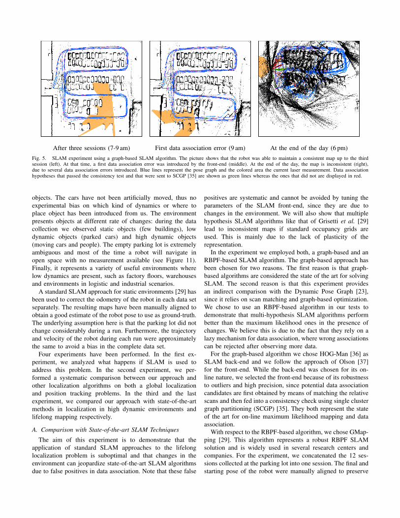
After three sessions (7-9 am) First data association error (9 am) At the end of the day (6 pm)Fig. 5. SLAM experiment using a graph-based SLAM algorithm. The picture shows that the robot was able to maintain a consistent map up to the thirdsession (left). At that time, a first data association error was introduced by the front-end (middle). At the end of the day, the map is inconsistent (right),due to several data association errors introduced. Blue lines represent the pose graph and the colored area the current laser measurement. Data associationhypotheses that passed the consistency test and that were sent to SCGP [35] are shown as green lines whereas the ones that did not are displayed in red.

objects. The cars have not been artificially moved, thus noexperimental bias on which kind of dynamics or where toplace object has been introduced from us. The environmentpresents objects at different rate of changes: during the datacollection we observed static objects (few buildings), lowdynamic objects (parked cars) and high dynamic objects(moving cars and people). The empty parking lot is extremelyambiguous and most of the time a robot will navigate inopen space with no measurement available (see Figure 11).Finally, it represents a variety of useful environments wherelow dynamics are present, such as factory floors, warehousesand environments in logistic and industrial scenarios.

A standard SLAM approach for static environments [29] hasbeen used to correct the odometry of the robot in each data setseparately. The resulting maps have been manually aligned toobtain a good estimate of the robot pose to use as ground-truth.The underlying assumption here is that the parking lot did notchange considerably during a run. Furthermore, the trajectoryand velocity of the robot during each run were approximatelythe same to avoid a bias in the complete data set.

Four experiments have been performed. In the first ex-periment, we analyzed what happens if SLAM is used toaddress this problem. In the second experiment, we per-formed a systematic comparison between our approach andother localization algorithms on both a global localizationand position tracking problems. In the third and the lastexperiment, we compared our approach with state-of-the-artmethods in localization in high dynamic environments andlifelong mapping respectively.

A. Comparison with State-of-the-art SLAM Techniques

The aim of this experiment is to demonstrate that theapplication of standard SLAM approaches to the lifelonglocalization problem is suboptimal and that changes in theenvironment can jeopardize state-of-the-art SLAM algorithmsdue to false positives in data association. Note that these false

positives are systematic and cannot be avoided by tuning theparameters of the SLAM front-end, since they are due tochanges in the environment. We will also show that multiplehypothesis SLAM algorithms like that of Grisetti et al. [29]lead to inconsistent maps if standard occupancy grids areused. This is mainly due to the lack of plasticity of therepresentation.

In the experiment we employed both, a graph-based and anRBPF-based SLAM algorithm. The graph-based approach hasbeen chosen for two reasons. The first reason is that graph-based algorithms are considered the state of the art for solvingSLAM. The second reason is that this experiment providesan indirect comparison with the Dynamic Pose Graph [23],since it relies on scan matching and graph-based optimization.We chose to use an RBPF-based algorithm in our tests todemonstrate that multi-hypothesis SLAM algorithms performbetter than the maximum likelihood ones in the presence ofchanges. We believe this is due to the fact that they rely on alazy mechanism for data association, where wrong associationscan be rejected after observing more data.

For the graph-based algorithm we chose HOG-Man [36] asSLAM back-end and we follow the approach of Olson [37]for the front-end. While the back-end was chosen for its on-line nature, we selected the front-end because of its robustnessto outliers and high precision, since potential data associationcandidates are first obtained by means of matching the relativescans and then fed into a consistency check using single clustergraph partitioning (SCGP) [35]. They both represent the stateof the art for on-line maximum likelihood mapping and dataassociation.

With respect to the RBPF-based algorithm, we chose GMap-ping [29]. This algorithm represents a robust RBPF SLAMsolution and is widely used in several research centers andcompanies. For the experiment, we concatenated the 12 ses-sions collected at the parking lot into one session. The final andstarting pose of the robot were manually aligned to preserve

continuity in the robot path. Both SLAM algorithms were thentested on the resulting data as it would have been a single robotrun.

Figure 5 shows the performance of the graph-based algo-rithm. The algorithm is able to correctly track the robot forthe first three sessions and estimates the correct trajectory anda consistent map of the environment (see the leftmost figure).This is also due to the fact that during the first two sessions,the environment did not change substantially, since few carswere parked there before 9 am. However, around 9 am mostof the people came to work and the parking lot configurationchanged. In the middle figure, we see that the front-endmistakenly added a loop closing transformation between tworobot poses, leading to an inconsistent map. Note that this isnot necessarily an error of the front end. The two observationswere really almost identical, since a car parked on a spot thatwas free in the previous sessions and the system matched itwith the car parked beside it. Finally, the rightmost figureshows the robot trajectory and the map at the end of the day(6 pm), when all data has been processed. As we can see, themap is highly inconsistent and the robot path wrong.

Please note that this performance violates one of the as-sumption made in DPG-SLAM [23], i.e., that the trajectoryestimation can be done using graph-based SLAM algorithmsin combination with scan matching for detecting loop clos-ing edges (more details on this assumption are provided inWalcott-Bryant’s PhD thesis [38], Chapter 4, Section 4.1.3).

This behavior of the system convinced us that to betteraddress this data association problem a multi hypothesesapproach was needed. To this end, we performed the sameexperiment using GMapping [29]. By tuning the number ofparticles, we were able to obtain a consistent map of theenvironment at the end. However, two limitations are stillpresent. Firstly, the algorithm was slower than the graph-based one and certainly not adapted to on-line navigation.This is mainly due to the number of particles needed and thecontinuous map updates. Note that this also impose memorylimitations, due to each hypothesis carrying its own map.Secondly, the update rate of the map strongly depended onhow often a certain cell has been already observed.

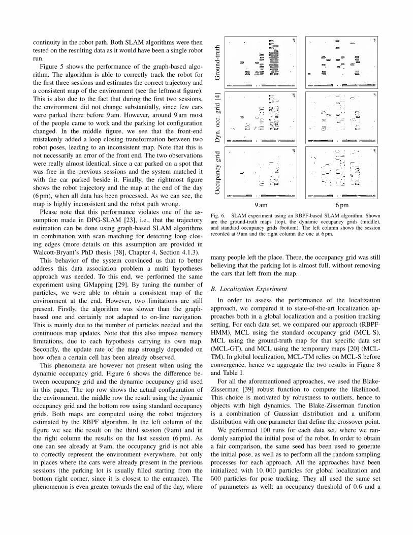
This phenomena are however not present when using thedynamic occupancy grid. Figure 6 shows the difference be-tween occupancy grid and the dynamic occupancy grid usedin this paper. The top row shows the actual configuration ofthe environment, the middle row the result using the dynamicoccupancy grid and the bottom row using standard occupancygrids. Both maps are computed using the robot trajectoryestimated by the RBPF algorithm. In the left column of thefigure we see the result on the third session (9 am) and inthe right column the results on the last session (6 pm). Asone can see already at 9 am, the occupancy grid is not ableto correctly represent the environment everywhere, but onlyin places where the cars were already present in the previoussessions (the parking lot is usually filled starting from thebottom right corner, since it is closest to the entrance). Thephenomenon is even greater towards the end of the day, where

Gro

und-

trut

hD

yn.o

cc.g

rid

[4]

Occ

upan

cygr

id

9 am 6 pmFig. 6. SLAM experiment using an RBPF-based SLAM algorithm. Shownare the ground-truth maps (top), the dynamic occupancy grids (middle),and standard occupancy grids (bottom). The left column shows the sessionrecorded at 9 am and the right column the one at 6 pm.

many people left the place. There, the occupancy grid was stillbelieving that the parking lot is almost full, without removingthe cars that left from the map.

B. Localization Experiment

In order to assess the performance of the localizationapproach, we compared it to state-of-the-art localization ap-proaches both in a global localization and a position trackingsetting. For each data set, we compared our approach (RBPF-HMM), MCL using the standard occupancy grid (MCL-S),MCL using the ground-truth map for that specific data set(MCL-GT), and MCL using the temporary maps [20] (MCL-TM). In global localization, MCL-TM relies on MCL-S beforeconvergence, hence we aggregate the two results in Figure 8and Table I.

For all the aforementioned approaches, we used the Blake-Zisserman [39] robust function to compute the likelihood.This choice is motivated by robustness to outliers, hence toobjects with high dynamics. The Blake-Zisserman functionis a combination of Gaussian distribution and a uniformdistribution with one parameter that define the crossover point.

We performed 100 runs for each data set, where we ran-domly sampled the initial pose of the robot. In order to obtaina fair comparison, the same seed has been used to generatethe initial pose, as well as to perform all the random samplingprocesses for each approach. All the approaches have beeninitialized with 10, 000 particles for global localization and500 particles for pose tracking. They all used the same setof parameters as well: an occupancy threshold of 0.6 and a

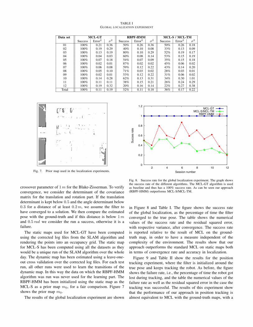
TABLE IGLOBAL LOCALIZATION EXPERIMENT

Data set MCL-GT RBPF-HMM MCL-S / MCL-TMSuccess Error2 σ2 Success Error2 σ2 Success Error2 σ2

01 100% 0.21 0.36 50% 0.26 0.36 50% 0.26 0.1802 100% 0.19 0.29 40% 0.10 0.08 33% 0.13 0.0903 100% 0.13 0.19 80% 0.10 0.29 52% 0.19 0.1704 100% 0.04 0.03 60% 0.08 0.14 53% 0.15 0.1905 100% 0.07 0.18 54% 0.07 0.09 35% 0.15 0.1806 100% 0.02 0.01 87% 0.02 0.02 45% 0.06 0.0207 100% 0.06 0.08 59% 0.12 0.22 43% 0.14 0.2008 100% 0.05 0.10 71% 0.03 0.02 28% 0.03 0.0109 100% 0.02 0.01 53% 0.12 0.22 31% 0.06 0.0210 100% 0.14 0.28 62% 0.13 0.31 34% 0.30 1.0111 100% 0.11 0.11 38% 0.15 0.21 26% 0.24 0.2912 100% 0.19 0.32 20% 0.16 0.14 22% 0.27 0.38

Total 100% 0.11 0.19 52% 0.11 0.18 36% 0.17 0.22

Fig. 7. Prior map used in the localization experiments.

crossover parameter of 1m for the Blake-Zisserman. To verifyconvergence, we consider the determinant of the covariancematrix for the translation and rotation part. If the translationdeterminant is kept below 0.5 and the angle determinant below0.3 for a distance of at least 0.2m, we assume the filter tohave converged to a solution. We then compare the estimatedpose with the ground-truth and if this distance is below 1mand 0.5 rad we consider the run a success, otherwise it is afailure.

The static maps used for MCL-GT have been computedusing the corrected log files from the SLAM algorithm andrendering the points into an occupancy grid. The static mapfor MCL-S has been computed using all the datasets as theywould be a unique run of the SLAM algorithm over the wholeday. The dynamic map has been estimated using a leave-one-out cross validation over the corrected log files. For each testrun, all other runs were used to learn the transitions of thedynamic map. In this way the data on which the RBPF-HMMalgorithm was run was never used for the learning part. TheRBPF-HMM has been initialized using the static map as theMCL-S as a prior map m0, for a fair comparison. Figure 7shows the prior map m0.

The results of the global localization experiment are shown

0

0.2

0.4

0.6

0.8

1

1.2

2 4 6 8 10 12

Succes r

ate

Session number

MCL-GT

MCL-S/MCL-TM

RBPF-HMM

Fig. 8. Success rate for the global localization experiment. The graph showsthe success rate of the different algorithms. The MCL-GT algorithm is usedas baseline and thus has a 100% success rate. As can be seen our approach(RBPF-HMM) outperforms MCL-S/MCL-TM.

in Figure 8 and Table I. The figure shows the success rateof the global localization, as the percentage of time the filterconverged to the true pose. The table shows the numericalvalues of the success rate and the residual squared error,with respective variance, after convergence. The success rateis reported relative to the result of MCL on the ground-truth map, in order to have a measure independent of thecomplexity of the environment. The results show that ourapproach outperforms the standard MCL on static maps bothin terms of convergence rate and accuracy in localization.

Figure 9 and Table II show the results for the positiontracking experiment, where the filter is initialized around thetrue pose and keeps tracking the robot. As before, the figureshows the failure rate, i.e., the percentage of time the robot gotlost during tracking, and the table the numerical values of thefailure rate as well as the residual squared error in the case thetracking was successful. The results of this experiment showthat the performance of our approach in position tracking isalmost equivalent to MCL with the ground-truth maps, with a

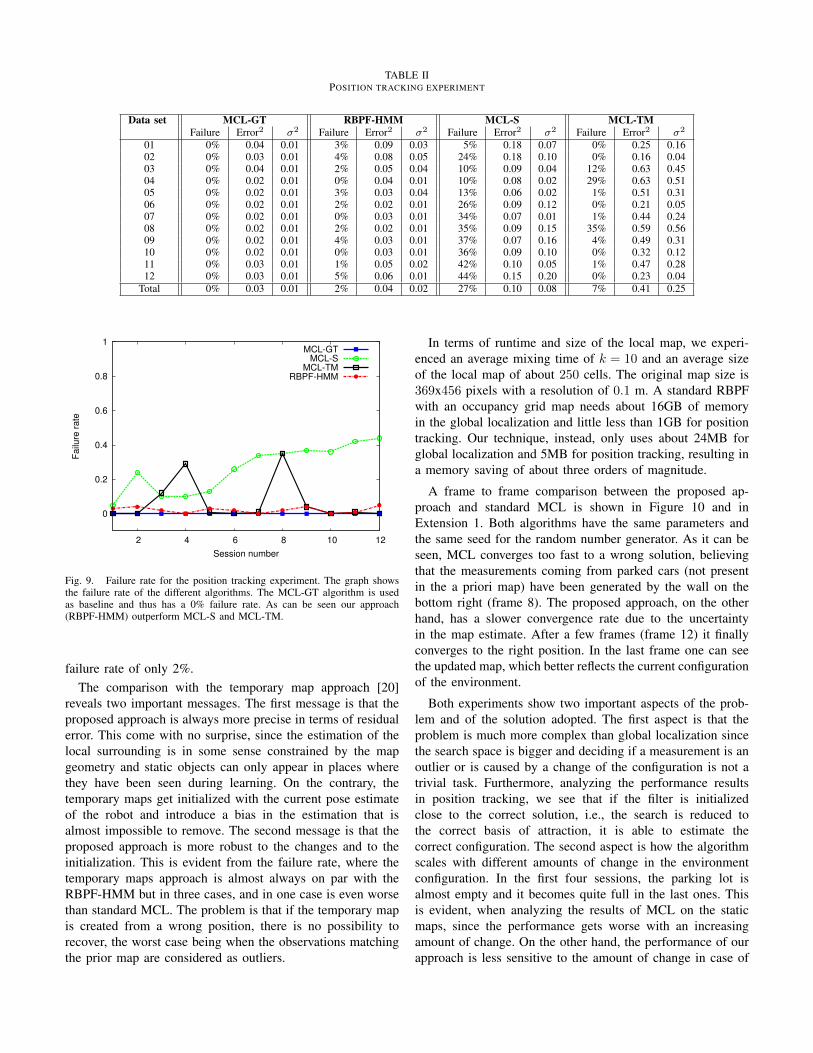
TABLE IIPOSITION TRACKING EXPERIMENT

Data set MCL-GT RBPF-HMM MCL-S MCL-TMFailure Error2 σ2 Failure Error2 σ2 Failure Error2 σ2 Failure Error2 σ2

01 0% 0.04 0.01 3% 0.09 0.03 5% 0.18 0.07 0% 0.25 0.1602 0% 0.03 0.01 4% 0.08 0.05 24% 0.18 0.10 0% 0.16 0.0403 0% 0.04 0.01 2% 0.05 0.04 10% 0.09 0.04 12% 0.63 0.4504 0% 0.02 0.01 0% 0.04 0.01 10% 0.08 0.02 29% 0.63 0.5105 0% 0.02 0.01 3% 0.03 0.04 13% 0.06 0.02 1% 0.51 0.3106 0% 0.02 0.01 2% 0.02 0.01 26% 0.09 0.12 0% 0.21 0.0507 0% 0.02 0.01 0% 0.03 0.01 34% 0.07 0.01 1% 0.44 0.2408 0% 0.02 0.01 2% 0.02 0.01 35% 0.09 0.15 35% 0.59 0.5609 0% 0.02 0.01 4% 0.03 0.01 37% 0.07 0.16 4% 0.49 0.3110 0% 0.02 0.01 0% 0.03 0.01 36% 0.09 0.10 0% 0.32 0.1211 0% 0.03 0.01 1% 0.05 0.02 42% 0.10 0.05 1% 0.47 0.2812 0% 0.03 0.01 5% 0.06 0.01 44% 0.15 0.20 0% 0.23 0.04

Total 0% 0.03 0.01 2% 0.04 0.02 27% 0.10 0.08 7% 0.41 0.25

0

0.2

0.4

0.6

0.8

1

2 4 6 8 10 12

Failure

rate

Session number

MCL-GT

MCL-S

MCL-TM

RBPF-HMM

Fig. 9. Failure rate for the position tracking experiment. The graph showsthe failure rate of the different algorithms. The MCL-GT algorithm is usedas baseline and thus has a 0% failure rate. As can be seen our approach(RBPF-HMM) outperform MCL-S and MCL-TM.

failure rate of only 2%.The comparison with the temporary map approach [20]

reveals two important messages. The first message is that theproposed approach is always more precise in terms of residualerror. This come with no surprise, since the estimation of thelocal surrounding is in some sense constrained by the mapgeometry and static objects can only appear in places wherethey have been seen during learning. On the contrary, thetemporary maps get initialized with the current pose estimateof the robot and introduce a bias in the estimation that isalmost impossible to remove. The second message is that theproposed approach is more robust to the changes and to theinitialization. This is evident from the failure rate, where thetemporary maps approach is almost always on par with theRBPF-HMM but in three cases, and in one case is even worsethan standard MCL. The problem is that if the temporary mapis created from a wrong position, there is no possibility torecover, the worst case being when the observations matchingthe prior map are considered as outliers.

In terms of runtime and size of the local map, we experi-enced an average mixing time of k = 10 and an average sizeof the local map of about 250 cells. The original map size is369x456 pixels with a resolution of 0.1 m. A standard RBPFwith an occupancy grid map needs about 16GB of memoryin the global localization and little less than 1GB for positiontracking. Our technique, instead, only uses about 24MB forglobal localization and 5MB for position tracking, resulting ina memory saving of about three orders of magnitude.

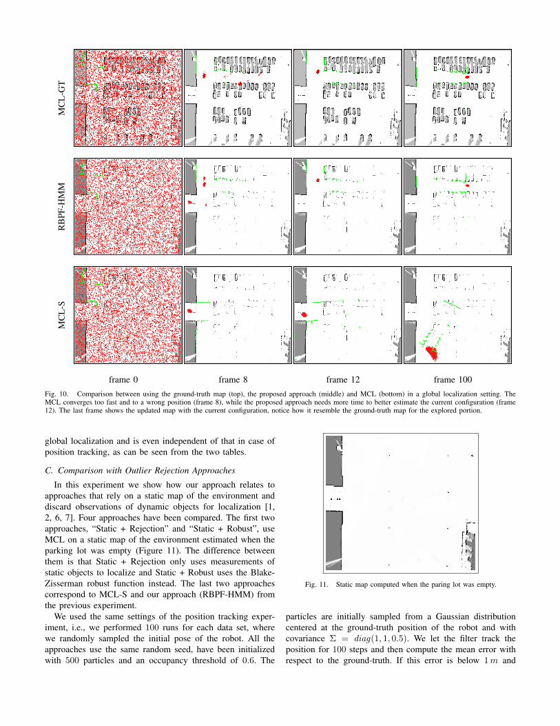
A frame to frame comparison between the proposed ap-proach and standard MCL is shown in Figure 10 and inExtension 1. Both algorithms have the same parameters andthe same seed for the random number generator. As it can beseen, MCL converges too fast to a wrong solution, believingthat the measurements coming from parked cars (not presentin the a priori map) have been generated by the wall on thebottom right (frame 8). The proposed approach, on the otherhand, has a slower convergence rate due to the uncertaintyin the map estimate. After a few frames (frame 12) it finallyconverges to the right position. In the last frame one can seethe updated map, which better reflects the current configurationof the environment.

Both experiments show two important aspects of the prob-lem and of the solution adopted. The first aspect is that theproblem is much more complex than global localization sincethe search space is bigger and deciding if a measurement is anoutlier or is caused by a change of the configuration is not atrivial task. Furthermore, analyzing the performance resultsin position tracking, we see that if the filter is initializedclose to the correct solution, i.e., the search is reduced tothe correct basis of attraction, it is able to estimate thecorrect configuration. The second aspect is how the algorithmscales with different amounts of change in the environmentconfiguration. In the first four sessions, the parking lot isalmost empty and it becomes quite full in the last ones. Thisis evident, when analyzing the results of MCL on the staticmaps, since the performance gets worse with an increasingamount of change. On the other hand, the performance of ourapproach is less sensitive to the amount of change in case of

MC

L-G

TR

BPF

-HM

MM

CL

-S

frame 0 frame 8 frame 12 frame 100Fig. 10. Comparison between using the ground-truth map (top), the proposed approach (middle) and MCL (bottom) in a global localization setting. TheMCL converges too fast and to a wrong position (frame 8), while the proposed approach needs more time to better estimate the current configuration (frame12). The last frame shows the updated map with the current configuration, notice how it resemble the ground-truth map for the explored portion.

global localization and is even independent of that in case ofposition tracking, as can be seen from the two tables.

C. Comparison with Outlier Rejection Approaches

In this experiment we show how our approach relates toapproaches that rely on a static map of the environment anddiscard observations of dynamic objects for localization [1,2, 6, 7]. Four approaches have been compared. The first twoapproaches, “Static + Rejection” and “Static + Robust”, useMCL on a static map of the environment estimated when theparking lot was empty (Figure 11). The difference betweenthem is that Static + Rejection only uses measurements ofstatic objects to localize and Static + Robust uses the Blake-Zisserman robust function instead. The last two approachescorrespond to MCL-S and our approach (RBPF-HMM) fromthe previous experiment.

We used the same settings of the position tracking exper-iment, i.e., we performed 100 runs for each data set, wherewe randomly sampled the initial pose of the robot. All theapproaches use the same random seed, have been initializedwith 500 particles and an occupancy threshold of 0.6. The

Fig. 11. Static map computed when the paring lot was empty.

particles are initially sampled from a Gaussian distributioncentered at the ground-truth position of the robot and withcovariance Σ = diag(1, 1, 0.5). We let the filter track theposition for 100 steps and then compute the mean error withrespect to the ground-truth. If this error is below 1m and

0

0.2

0.4

0.6

0.8

1

1.2

2 4 6 8 10 12

Failu

re r

ate

Session number

Static + RejectionStatic + Robust

MCL-SRBPF-HMM

Fig. 12. Failure rate for the outlier rejection experiment. The graph showsthe failure rate of the different algorithms. The figure clearly show that outlierrejection mechanisms are more sensitive to changing environments than therobust likelihood function. It also show our approach outperforms techniquesbased on outlier rejections.

0.5 rad we consider the run a success, otherwise it is a failure.Figure 12 depicts the results of the experiment. As in the

position tracking experiment, the figure shows the failure rate,i.e., the percentage of time the robot got lost during tracking.From the plot and the static map, we can see two clearmessages. The first message is that outlier rejection mechanismare more sensitive to changes in the environment when nostatic part of the environment is visible. This is clear if onecompares the performances of Static + Rejection with Static+ Robust.

The second message is that the static portion of the envi-ronment does not contain enough information for the robotto localize itself and observations of low dynamic objectsimprove localization. This is visible in the plot: our approach(RBPF-HMM) has a better performance than MCL-S, whichin turn has a better performance than Static + Robust. Allthe approaches use the same likelihood function and the samealgorithm, the only difference is the amount of informationstored in the map with respect to objects with low dynamics.For the static map case, no information about the low dynamicobjects is present. In the MCL-S case, objects that have beenobserved most of the time are present in the map, due to theoccupancy grid update rule. In our approach, the dynamics ofthose objects are explicitly modeled in the dynamic occupancygrids. This allows us to infer how often we expect to see alow dynamic object in the environment and for how long.

D. Comparison with Lifelong Mapping using Experiences

The aim of this experiment is to compare the performance ofour approach with the experience map of Churchill and New-man [24], a state-of-the-art method for lifelong mapping. Inthe experience map approach, the environment is representedby a set of experiences, where each experience is a sequence ofobservations connected by visual odometry. During operation,each experience is equipped with a localizer whose task is to

0

0.2

0.4

0.6

0.8

1

2 4 6 8 10 12

Norm

aliz

ed o

dom

etr

y o

utp

ut added to m

ap

(F

ailu

re r

ate

)

Session number

Churchill and Newmann, N=1Churchill and Newmann, N=2Churchill and Newmann, N=3

RBPF-HMM

0

0.2

0.4

0.6

0.8

1

2 4 6 8 10 12

Norm

aliz

ed o

dom

etr

y o

utp

ut added to m

ap

(F

ailu

re r

ate

)

Session number

Churchill and Newmann, N=1Churchill and Newmann, N=2Churchill and Newmann, N=3

RBPF-HMM

Fig. 13. Results for the lifelong mapping experiment using the generousthresholds (top) and the more restrictive ones (bottom). The plots show thenormalized odometry output added to the map for the approach of Churchilland Newman [24], which is equivalent of the failure rate of the positiontracking. For the sake of comparison we also plot the performances of ourapproach. The plot shows that our approach has a better performance even inthe case when a single experience is needed for localization.

track the position of the robot in the experience, or declareit “lost” in case of tracking failure. When the system isnot able to localize the robot in at least N experiences, thecurrent observation sequence becomes a new experience andis inserted in the map. The approach relies on two maincomponents: the ability to “close a loop”, i.e., to globallylocalize the robot and the ability to navigate locally, i.e., theability to track the position of the robot. We use the ground-truth position to initialize the localizers of every experienceand the MCL algorithm to track the position, since they bothwork reliably in the case where no changes are present inenvironment.

For each data set, we consider all other datasets as previousexperiences and performed the same 100 runs that were usedin the position tracking experiment. For each run, all thelocalizers for every other experience are initialized with aGaussian distribution centered at the ground-truth position ofthe robot and with covariance Σ = diag(1, 1, 0.5). We trackthe position for 100 steps and check how many times the

localizers declared the robot as “lost”. For a fair comparison,we used the same thresholds of 1m and 0.5 rad to check thesuccess of position tracking. To give a better picture aboutthe performances of the two approaches, we also performan additional experiment using tighter thresholds: 0.2m and0.1 rad .

Figure 13 shows the normalized odometry output addedto the map for different values of N , the minimum numberof successful localizers. Note that this number is equivalentto the failure rate of the system to localize the robot, sincenew experiences are added in case of localization failures.For the sake of comparison, we also included the failurerate of our approach in the same settings. Note that weused on purpose the same runs and the same algorithm forposition tracking to have a fair comparison. We also usedthe same amount of information about the environment, i.e.,all the datasets/experiences not used for the testing run. Theonly difference in the two approaches is the environmentrepresentation and the way inference over the environment isperformed.

The plot shows that our approach has the best performance,with the experience map relying only on a single localizer hav-ing a similar performance. Increasing the number of requiredlocalizers, drastically decreases the performance of the system.We believe this is due to the local nature of the changes in theparking lot. Note that the same phenomena have been reportedin the original paper, where the car park was in one of theregions with high variation. If we analyze the bottom plot withthe tighter thresholds, we see that the gap in performancesbetween our approach and the experience map increases. Webelieve this is due to the fact that the stored maps do notfully represent the current configuration of the environment,resulting in higher error in localization. Our approach, instead,is able to generalize better to unseen environments and can stillachieve high localization accuracy.

The computational complexity of the experience map ismuch higher than in our approach. We only require onelocalizer and the local update of the map, where the experiencemap requires one localizer for each experience. Hence, ourapproach scales with the environment size while their approachscales with the environment size and the number of differentconfigurations.

The experiment also provides an indirect comparison withthe approach of Stachniss and Burgard [19], since it is a specialcase of the experience map, in case a particle filter is used aslocalizer and only one experience is needed for localization.

VII. CONCLUSIONS

In this paper, we presented a probabilistic localizationframework for robots operating in dynamic environments. Ourapproach recursively estimates not only the pose of the robot,but also the state of the environment. It employs a hiddenMarkov model to represent the dynamics of the environmentand a Rao-Blackwellized particle filter to efficiently estimatethe joint state. In addition, it exploits the properties of Markov

chains to reduce the memory requirements so that the al-gorithm can be run online on a real robot. Our approachhas two advantages. First, it allows for accurate and robustlocalization even in changing environments and, second, itprovides up-to-date maps of them. We evaluated our algorithmextensively using real-world data. The results demonstratethat our model substantially outperforms the popular Monte-Carlo localization algorithm. This makes our method moresuitable for long-term operation of mobile robots in changingenvironments.

In future, we would like to extend our model to reasonabout objects and not only about individual cells. We will fur-thermore investigate alternative models to encode the changes(e.g., Dynamic Bayesian Networks and second order hiddenMarkov models). This will provide a novel perspective on howto reason about correlations in a grid map. In addition, we planto look further into the detection of moving object and motionsegmentation.

We also plan on releasing the software package implement-ing the approach described in this article as open source andon making the datasets used available at publication time.

ACKNOWLEDGMENT

This work has been partially supported by the EuropeanCommission under contract numbers FP7-248258-FirstMM,FP7-260026-TAPAS and ERC-267686-LifeNav.

REFERENCES

[1] D. Fox, W. Burgard, and S. Thrun, “Markov localizationfor mobile robots in dynamic environments,” Journal ofArtificial Intelligence Research, vol. 11, 1999.

[2] D. Schulz, D. Fox, and J. Hightower, “Peopletracking with anonymous and id-sensors using rao-blackwellised particle filters,” in Proc. of the Int. Conf. onArtificial Intelligence (IJCAI), 2003. [Online]. Available:http://dl.acm.org/citation.cfm?id=1630659.1630792

[3] D. Hahnel, R. Triebel, W. Burgard, and S. Thrun, “Mapbuilding with mobile robots in dynamic environments,”in Proc. of the IEEE Int. Conf. on Robotics & Automation(ICRA), 2003.

[4] D. Meyer-Delius, M. Beinhofer, and W. Burgard, “Oc-cupancy grid models for robot mapping in changingenvironments,” in Proc. of the AAAI Conf. on ArtificialIntelligence (AAAI), Toronto, Canada, July 2012.

[5] M. Montemerlo, S. Thrun, and W. Whittaker, “Con-ditional particle filters for simultaneous mobile robotlocalization and people-tracking,” in Proc. of the IEEEInt. Conf. on Robotics & Automation (ICRA), 2002.

[6] D. F. Wolf and G. S. Sukhatme, “Mobile robot simultane-ous localization and mapping in dynamic environments,”Autonomous Robots, vol. 19, no. 1, pp. 53–65, 2005.

[7] C.-C. Wang, C. Thorpe, S. Thrun, M. Hebert, andH. Durrant-Whyte, “Simultaneous localization, mappingand moving object tracking,” International Journal ofRobotics Research (IJRR), 2007.

[8] L. Montesano, J. Minguez, and L. Montano, “Modelingthe static and the dynamic parts of the environment toimprove sensor-based navigation,” in Proc. of the IEEEInt. Conf. on Robotics & Automation (ICRA), 2005.

[9] G. Gallagher, S. S. Srinivasa, J. A. Bagnell, and D. Fer-guson, “GATMO: A generalized approach to trackingmovable objects,” in Proc. of the IEEE Int. Conf. onRobotics & Automation (ICRA), 2009.

[10] D. Anguelov, R. Biswas, D. Koller, B. Limketkai, S. San-ner, and S. Thrun, “Learning hierarchical object mapsof non-stationary environments with mobile robots,” inProc. of the Conference on Uncertainty in AI (UAI),2002.

[11] C. Chen, C. Tay, C. Laugier, and K. Mekhnacha, “Dy-namic environment modeling with gridmap: A multiple-object tracking application,” in Proc. of the IEEEInt. Conf. on Control, Automation, Robotics and Vision(ICARCV), 2006.

[12] S. Brechtel, T. Gindele, and R. Dillmann, “Recursiveimportance sampling for efficient grid-based occupancyfiltering in dynamic environments,” in Proc. of the IEEEInt. Conf. on Robotics & Automation (ICRA), 2010.

[13] P. Biber and T. Duckett, “Dynamic maps for long-termoperation of mobile service robots,” in Proc. of Robotics:Science and Systems (RSS), 2005.

[14] S.-W. Yang and C.-C. Wang, “Feasibility grids for local-ization and mapping in crowded urban scenes,” in IEEEInternational Conference on Robotics and Automation(ICRA), Shanghai, China, May 2011.

[15] J. Saarinen, H. Andreasson, and A. J. Lilienthal, “In-dependent markov chain occupancy grid maps for rep-resentation of dynamic environments,” in Proc. of theIEEE/RSJ Int. Conf. on Intelligent Robots and Systems(IROS), 2012.

[16] K. Murphy, “Bayesian map learning in dynamic envi-ronments,” in Proc. of the Conf. on Neural InformationProcessing Systems (NIPS), Denver, CO, USA, 1999, pp.1015–1021.

[17] D. Avots, E. Lim, R. Thibaux, and S. Thrun, “A proba-bilistic technique for simultaneous localization and doorstate estimation with mobile robots in dynamic environ-ments,” in Proc. of the IEEE/RSJ Int. Conf. on IntelligentRobots and Systems (IROS), 2002.

[18] A. Petrovskaya and A. Y. Ng, “Probabilistic mobilemanipulation in dynamic environments, with applicationto opening doors,” in Proc. of the Int. Conf. on ArtificialIntelligence (IJCAI), 2007.

[19] C. Stachniss and W. Burgard, “Mobile robot mappingand localization in non-static environments,” in Proc. ofthe Nat. Conf. on Artificial Intelligence (AAAI), 2005.

[20] D. Meyer-Delius, J. Hess, G. Grisetti, and W. Burgard,“Temporary maps for robust localization in semi-staticenvironments,” in Proc. of the IEEE/RSJ InternationalConference on Intelligent Robots and Systems (IROS),Taipei, Taiwan, 2010.

[21] K. Konolige and J. Bowman, “Towards lifelong visual

maps,” in Proc. of the IEEE/RSJ Int. Conf. on IntelligentRobots and Systems (IROS), 2009.

[22] H. Kretzschmar and C. Stachniss, “Information-theoreticcompression of pose graphs for laser-based slam,” Inter-national Journal of Robotics Research (IJRR), vol. 31,2012.

[23] A. Walcott-Bryant, M. Kaess, H. Johannsson, andJ. Leonard, “Dynamic pose graph SLAM: Long-termmapping in low dynamic environments,” in Proc. of theIEEE/RSJ Int. Conf. on Intelligent Robots and Systems(IROS), Vilamoura, Portugal, 2012.

[24] W. Churchill and P. Newman, “Practice makes perfect?managing and leveraging visual experiences for lifelongnavigation,” in Proc. of the IEEE Int. Conf. on Robotics& Automation (ICRA), 2012, pp. 4525 –4532.

[25] G. Grisetti, R. Kummerle, C. Stachniss, and W. Burgard,“A tutorial on graph-based SLAM,” IEEE Transactionson Intelligent Transportation Systems Magazine, vol. 2,pp. 31–43, 2010.

[26] J. Rowekamper, C. Sprunk, G. D. Tipaldi, S. Cyrill,P. Pfaff, and W. Burgard, “On the position accuracyof mobile robot localization based on particle filterscombined with scan matching,” in Proceedings of theIEEE/RSJ International Conference on Intelligent Robotsand Systems (IROS), Villamoura, Protugal, 2012.

[27] H. Moravec and A. Elfes, “High resolution maps fromwide angle sonar,” in Proc. of the IEEE Int. Conf. onRobotics & Automation (ICRA), 1985.

[28] L. Rabiner, “A tutorial on hidden Markov models andselected applications in speech recognition.” in Proceed-ings of the IEEE, vol. 77 (2), 1989, pp. 257–286.

[29] G. Grisetti, C. Stachniss, and W. Burgard, “ImprovedTechniques for Grid Mapping with Rao-BlackwellizedParticle Filters,” IEEE Transactions on Robotics, vol. 23,no. 1, pp. 34–46, 2007.

[30] A. Doucet, J. de Freitas, K. Murphy, and S. Russel, “Rao-Blackwellized partcile filtering for dynamic bayesian net-works,” in Proc. of the Conf. on Uncertainty in ArtificialIntelligence (UAI), Stanford, CA, USA, 2000, pp. 176–183.

[31] S. Thrun, “A probabilistic online mapping algorithmfor teams of mobile robots,” International Journal ofRobotics Research (IJRR), vol. 20, no. 5, pp. 335–363,2001.

[32] D. A. Levin, Y. Peres, and E. L. Wilmer, Markov Chainsand Mixing Times. American Mathematical Society,2008.

[33] A. I. Eliazar and R. Parr, “Dp-slam 2.0,” in Proc. of theIEEE Int. Conf. on Robotics & Automation (ICRA), 2004.

[34] D. Fox, “Adapting the sample size in particle filtersthrough kld-sampling,” International Journal of RoboticsResearch (IJRR), vol. 22, 2003.

[35] E. Olson, M. Walter, J. Leonard, and S. Teller, “Singlecluster graph partitioning for robotics applications,” inProceedings of Robotics Science and Systems, 2005.

[36] G. Grisetti, R. Kummerle, C. Stachniss, U. Frese, and

C. Hertzberg, “Hierarchical optimization on manifoldsfor online 2d and 3d mapping,” in Proc. of the IEEEInt. Conf. on Robotics & Automation (ICRA), 2010.

[37] E. Olson, “Robust and efficient robotic mapping,” Ph.D.dissertation, Massachusetts Institute of Technology, Cam-bridge, MA, USA, June 2008.

[38] A. Walcott, “Long-term mobile robot mapping in dy-namic environments,” Ph.D. dissertation, MassachusettsInstitute of Technology, Cambridge, MA, USA, May2011.

[39] A. Blake and A. Zisserman, Visual reconstruction. Cam-bridge, MA, USA: MIT Press, 1987.

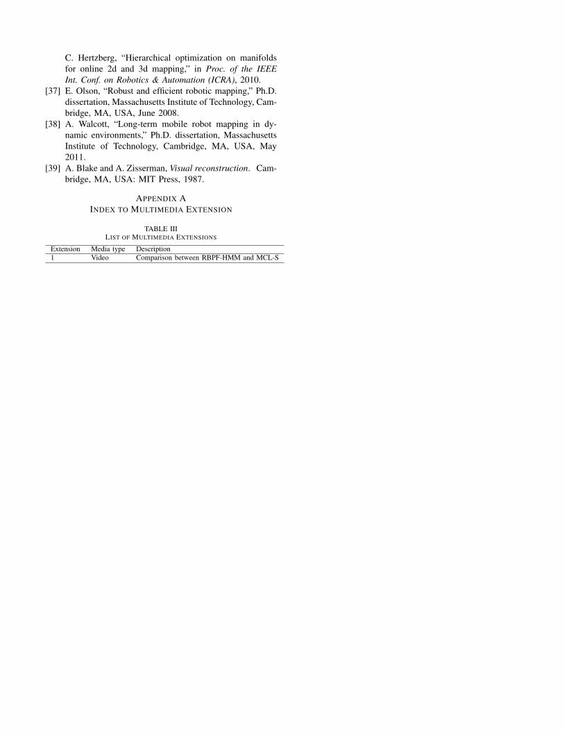
APPENDIX AINDEX TO MULTIMEDIA EXTENSION

TABLE IIILIST OF MULTIMEDIA EXTENSIONS

Extension Media type Description1 Video Comparison between RBPF-HMM and MCL-S