life-cycle equilibrium unemploymentftp.iza.org/dp3396.pdf · life-cycle equilibrium unemployment...
TRANSCRIPT

IZA DP No. 3396
Life-Cycle Equilibrium Unemployment
Arnaud ChéronJean-Olivier HairaultFrançois Langot
DI
SC
US
SI
ON
PA
PE
R S
ER
IE
S
Forschungsinstitutzur Zukunft der ArbeitInstitute for the Studyof Labor
March 2008
Life-Cycle Equilibrium Unemployment
Arnaud Chéron University of Maine (GAINS)
and EDHEC
Jean-Olivier Hairault Paris School of Economics (PSE),
University of Paris I and IZA
François Langot PSE-Jourdan, CEPREMAP,
University of Maine (GAINS) and IZA
Discussion Paper No. 3396 March 2008
IZA
P.O. Box 7240 53072 Bonn
Germany
Phone: +49-228-3894-0 Fax: +49-228-3894-180
E-mail: [email protected]
Any opinions expressed here are those of the author(s) and not those of IZA. Research published in this series may include views on policy, but the institute itself takes no institutional policy positions. The Institute for the Study of Labor (IZA) in Bonn is a local and virtual international research center and a place of communication between science, politics and business. IZA is an independent nonprofit organization supported by Deutsche Post World Net. The center is associated with the University of Bonn and offers a stimulating research environment through its international network, workshops and conferences, data service, project support, research visits and doctoral program. IZA engages in (i) original and internationally competitive research in all fields of labor economics, (ii) development of policy concepts, and (iii) dissemination of research results and concepts to the interested public. IZA Discussion Papers often represent preliminary work and are circulated to encourage discussion. Citation of such a paper should account for its provisional character. A revised version may be available directly from the author.

IZA Discussion Paper No. 3396 March 2008
ABSTRACT
Life-Cycle Equilibrium Unemployment*
This paper develops a life-cycle approach to equilibrium unemployment. Workers only differ respectively to their distance from deterministic retirement. A non age-directed search equilibrium is then typically featured by increasing (decreasing) firing (hiring) rates with age and a hump-shaped age profile for employment. Because of intergenerational inefficiencies, the Hosios condition no longer achieves efficiency. We then explore the optimal age-pattern of some policy tools to restore this efficiency. The optimal profile for employment subsidies should increase with age, whereas firing taxes and hirings subsidies would have to be hump-shaped. Lastly, we examine the robustness of our results. We show that age-directed recruitment policies cannot exist in equilibrium even if it would have been ex-ante possible, and that introducing endogenous search effort of unemployed workers reinforces our main results. JEL Classification: J22, J26, H55 Keywords: job search, matching, life cycle Corresponding author: Jean-Olivier Hairault EUREQua University of Paris I 106-112, Boulevard de l'Hôpital 75647 Paris Cedex 13 France E-mail: [email protected]
* We thank the participants at the SED congress (Vancouver, 2006), and the IUI (Stockholm, 2006) and Pennsylvania seminars (Philadelphia, 2007) for helpful comments.

1 IntroductionSince Oi [1962], labor is conventionally viewed as a quasi-�xed input factor.The hiring process is costly and �rms implement labor hoarding strategies:forward looking decisions of hiring and �ring depend on the time over whichto recoup adjustment costs. A major contribution of the extensively usedframework of Mortensen and Pissarides [1994] (MP hereafter) is to providetheoretical foundations to these mechanisms in a overall theory of equilib-rium unemployment with matching frictions and wage bargaining. In thatcontext, endogenous hirings and separations depend on expected durationof jobs. Surprisingly enough, the life cycle of workers has not been yet in-corporated in equilibrium unemployment models whereas this duration isobviously tightly related to the distance from worker's retirement. This is asmuch surprising as the relation between the labor supply and the life cyclewas already pointed out since the seminal Heckman [1974] and MaCurdy[1981] papers. Seater [1974], Hutchens [1988] and more recently Lunqjvistand Sargent [2002] also emphasized the role played by the life cycle in thesearch decision of unemployed workers, both from theoretical and empiricalstandpoints. This paper aims at �lling this gap by examining positive andnormative issues related to the introduction of the life cycle in the theory ofequilibrium unemployment.
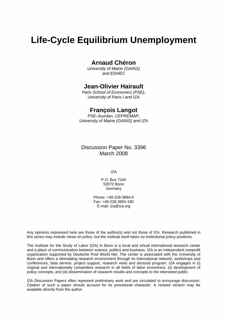
Traditionally, the labor market equilibrium is analyzed by taking intoaccount speci�c labor market institutions like employment protection (Blan-chard and Portugal [2001]), unemployment insurance (Lunqvist and Sargent[2004]) or tax system and government (Prescott [2004], Rogerson [2006]).These studies do not recognize the employment di�erences by age as central.In this paper, we put forward the idea that adopting a life cycle view mayenhance our understanding of the labor market equilibrium. Indeed, Figure1 shows �rstly that employment rates di�er across ages whatever the coun-try considered. The age-dynamics of employment is hump-shaped: youngerand older workers display lower employment rates. Secondly, as can be seenin �gure 1, employment rate di�erences across countries seem to be concen-trated at particular ages: there exists large heterogeneity of employment ratesamong OECD countries for the youngest and the oldest workers1, whereasthe employment rates for workers between 30 and 50 years old are very lowdispersed (see also OECD [2006]).
In this paper, we aim at showing that the canonical MP model augmentedby life cycle features naturally delivers outcomes which are qualitatively in
1Note that we consider employment rates for people aged of less than 60 years in orderto not capture di�erences in labor participation due to di�erent normal retirement ages.
2
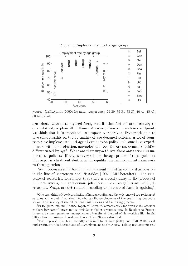
Figure 1: Employment rates by age groups
20 30 40 50 6040
50
60
70
80
90
100Employment rate by age group
Age group
Em
ploy
men
t rat
e in
%
Bel
Can
Ger
Den
Spa
Fin
Fra
UK
Ita
Jap
Swe
US
Source: OECD data (2000) for men. Age groups: 25-29, 30-34, 35-39, 40-44, 45-49,50-54, 55-59.
accordance with these stylized facts, even if other factors2 are necessary toquantitatively explain all of them. Moreover, from a normative standpoint,we think that it is important to propose a theoretical framework able togive some insights on the optimality of age-designed policies. A lot of coun-tries have implemented anti-age discrimination policy and some have experi-mented with job protection, unemployment bene�ts or employment subsidiesdi�erentiated by age3. What are their impact? Are there any rationales un-der these policies? If any, what would be the age pro�le of these policies?Our paper is a �rst contribution in the equilibrium unemployment frameworkto these questions.
We propose an equilibrium unemployment model as standard as possiblein the line of Mortensen and Pissarides [1994] (MP hereafter). The exis-tence of search frictions imply that there is a costly delay in the process of�lling vacancies, and endogenous job destructions closely interact with jobcreations. Wages are determined according to a standard Nash bargaining4.
2One may think of the depreciation of human capital and the existence of pre-retirementsystems at the end of working life, whereas the employment of the youth may depend alot on the e�ciency of the educational institutions and the hiring process.
3In Belgium, Finland, France Japan or Korea, it is more costly for �rms to lay o� olderworkers because of longer notice periods or higher severance pay. In Belgium or France,there exists more generous unemployment bene�ts at the end of the working life. In theUK or France, hirings of workers of more than 50 are subsidized.
4This approach has been recently criticized by Shimer [2005] and Hall [2005] as itunderestimates the �uctuations of unemployment and vacancy. Taking into account real
3

Contrary to the large literature following MP, we consider a life cycle settingcharacterized by a deterministic age at which workers exit the labor market.There is no more heterogeneity than the distance to retirement. We considerthat this is a natural starting point to which other potential sources of het-erogeneity across workers of di�erent ages could be added5. We also considerin our benchmark economy that �rms cannot ex-ante age-direct their search,that is vacancies cannot be targeted on a speci�c age group as the resultof the legislation prohibiting age-discrimination6. Consistently, unemployedworkers are randomly matched with available job vacancies irrespective oftheir age.
The �rst contribution of this paper is to reveal the direct in�uence ofimpending retirement on both job creations and destructions. We show thatextending MP's framework to account for a deterministic exit date from thelabor market naturally deliver a hump-shaped age-dynamics of employment.On the one hand, because the horizon of older workers is shorter, we showthat �rms invest less in labor-hoarding activities at the end of the life cycle.This implies that the �ring (hiring) rate increases (decreases) with the ageof the worker, so that the employment rate is falling at the end of the life-cycle. We argue that di�erences in retirement ages can account for observeddi�erences in employment rates of older workers: more or less longer horizonof the worker on the labor market appears as a key variable to understandeither smoother or sharper decrease in the employment rate from 50 yearsold on. On the other hand, since new entrants are unemployed, low �ringrates at the beginning of the working life cycle make the employment rateincreasing with age until a threshold age.
If the low employment rate of older workers can be explained by theshort horizon created by the coming retirement, the next issue is then toexamine the social optimality of such outcomes. Before engineering anypolicy devices to circumvent �rms to discriminate against older workers, itis necessary to study the social optimality of such behaviors. In the contextwage rigidities as suggested by Shimer [2005] and Hall [2005] would exacerbate the lifecycle impact on job �ows as emphasized in section 1.
5For instance, one could think that older workers have much more job-speci�c skills andsu�er more from separations. The amount of idiosyncratic uncertainty could be weakerfor older workers. The bargaining power of younger and older workers is not necessary thesame...
6This legislation in the US dates back to the 60's (Age Discrimination in EmploymentAct in 1967, and subsequent amendments). In 2000, the European Union Council Directivealso requires all 15 EU countries to introduce legislation prohibiting direct and indirectdiscrimination at work on the grounds of age.
4

of matching frictions and wage bargaining, it is now well-established thatthe decentralized equilibrium is in general not optimal, except when theHosios condition holds.7 In the life-cycle equilibrium, as �rms are engagedin a non age-directed search, the age distribution of the unemployed workersdetermines the return of vacancies. Older worker job destructions exert anegative externality on the employment of the younger unemployed workerswhich is not internalized by �rms in the decentralized equilibrium. This iswhy the Hosios condition is not enough to restore the social optimality ofthe life-cycle equilibrium: there are too much (not enough) older (younger)worker job destructions even though the optimal pro�le of job destructionsis increasing with age as in the equilibrium outcome.
We then de�ne the policies which could restore the e�ciency of the de-centralized equilibrium. We expect that the intergenerational externalitiesmay be corrected by policies designed by age. More speci�cally, older workerjob destructions must be reduced in order to limit the number of older un-employed workers likely to be contacted by �rms. We show that the optimaldesign of employment subsidies is increasing with age: older worker jobs arethe more subsidized whereas younger worker jobs are even taxed. Optimal�ring and hiring policies could also be implemented, but in a more complexway. Indeed, the sensitivity of �rm's �ring policy with respect to employ-ment protection is age-dependent. Namely, �ring taxes are more e�cient inthe last stages of the life cycle when �rms have strong incentives to wait forolder worker retirement as a way of escaping from �ring taxes. More pre-cisely, at the end of the working cycle, introducing a �ring tax increases thepresent �ring cost without any future consequences on the job value as theworker will be retired in the next period. On the opposite, for a youngerworker, the �ring decision depends not only on the current tax but also onthe expected one. We show that, everything being equal, this would requirethe age-dynamics of the �ring tax to be decreasing. Combining this e�ectwith the intergenerational externality leads to a hump-shaped feature for theoptimal age-dynamics of the �ring taxes, hence of hiring subsidies.
Lastly, in order to assess the scope of these results, we test the robust-ness of our model's implications with respect to the assumption of non-agedirected search and constant search e�ort for unemployed workers. First,we show that even though age-directed recruiting policies was possible, theequilibrium would feature only non-directed recruitment policies. This result
7This condition states that the elasticity of the matching friction with respect to vacan-cies should be equal to worker's bargaining power (Hosios [1990]). This e�ciency resultcould also be obtained in a competitive search equilibrium (Moen [1997]).
5

is tightly related with the assumption that there is no age-dependent abilityrequirement associated with a vacant position. This actually implies that allunemployed workers, whatever their age, are eager to apply to age-directedvacant positions, so that in equilibrium only non-directed recruitment policiesexist. Secondly, as unemployed search e�ort corresponds to an investment,we show that it adds another force to explain why older worker employmentmay be lower due to a shorter horizon. Unemployed older workers exhibita lower search e�ort than younger workers. Interestingly, this pro�le is alsopresent in the social optimum. Furthermore, the social return of older workersearch is not only lower due to the shorter horizon, as it is perceived by work-ers, but it also negatively impacts the return of �rm vacancies. This is whythe pro�le of unemployment search subsidies should be decreasing with age.The older worker search is less worthy to be encouraged as it exerts a partic-ularly negative externality on the younger unemployed workers by loweringthe job vacancies in the economy.
The remaining of the paper is organized as follows. A �rst section de-scribes the model and discusses equilibrium properties as regard with someempirical facts. The second section turns to e�ciency and labor policy is-sues. A third section is devoted to the robustness analysis. A last sectionconcludes the paper.
2 Equilibrium Life Cycle Dynamics of Job Cre-ations and Job Destructions
Let us consider an economy à la Mortensen - Pissarides [1994]. Labor marketfrictions imply that there is a costly delay in the process of �lling vacancies,and endogenous job destructions closely interact with job creations. Con-trary to the large literature following MP, we consider a life cycle settingcharacterized by a deterministic age at which workers exit the labor market.
2.1 Model EnvironmentWe consider a discrete time model and assume that at each period the olderworker generation retiring from the labor market is replaced by a youngerworker generation of the same size (normalized to unity) so that there is nolabor force growth in the economy. We denote i the worker's age and T theexogenous age at which workers exit the labor market: they are both perfectlyknown by employers. There is no other heterogeneity across workers. Theeconomy is at steady-state, and we do not allow for any aggregate uncertainty.
6

We assume that each worker of the new generation enters the labor marketas unemployed.
2.1.1 ShocksFirms are small and each has one job. The destruction �ows derive fromidiosyncratic productivity shocks that hit the jobs at random. Once a shockarrives, the �rm has no choice but either to continue production or to destroythe job. Then, for age i ∈ (2, T − 1), employed workers are faced withlayo�s when their job becomes unpro�table. At the beginning of each age8,a job productivity ε is drawn in the general distribution G(ε) with ε ∈ [0, ε].The �rms decide to close down any jobs whose productivity is below an(endogenous) productivity threshold (productivity reservation) denoted Ri.Job creation takes place when a �rm and a worker meet. The �ow of newlycreated jobs result from a matching function the inputs of which are vacanciesand unemployed workers. This �ow also depends on productivity thresholdsRi because it is assumed that productivity values ε are known after �rm andworker met.
2.1.2 Workers �ows with non age-directed searchWe assume that �rms cannot ex-ante age-direct their search and that thematching function embodies all unemployed workers. Let u be the numberof unemployment workers, v the vacancies, and assume at this stage thatworker search e�ort is exogenous. There is a matching function that givesthe number of hirings as a function of the number of vacancies and thenumber of unemployed workers, M(v, u), where M is increasing and concavein both its arguments, and with constant returns-to-scale. Let θ = v/udenote the tightness of the labor market. It is then straightforward to de�nethe probability for unemployed workers of age i to be employed at age i + 1,as jci ≡ p(θ)[1 − G(Ri+1)] with p(θ) = M(u,v)
u. Similarly, we de�ne the job
destruction rate for an employed worker of age i as jdi = G(Ri).At the beginning of their age i, the realization of the productivity level
on each job is revealed. Workers hired when they were i − 1 years old (atthe end of the period) are now productive. Workers whose productivity isbelow the reservation productivity Ri are either laid o� or not hired (forthose previously unemployed). For any age i, the �ow from employment tounemployment is then equal to G(Ri)(1 − ui−1). The other workers who
8This assumption is done to allow for analytical results. Persistency of shocks is leavedfor a quantitative empirical investigation of the model performance.
7

remain employed (1 − G(Ri))(1 − ui−1) can renegotiate their wage. Theage-dynamics of unemployment is then given by:
ui+1 = ui [1− p(θ)(1−G(Ri+1))] + G(Ri+1)(1− ui) ∀i ∈ (1, T − 1) (1)
for a given initial condition u1 = 1. The overall level of unemployment isu =
∑T−1i=1 ui, so that the average unemployment rate is u/[T − 1].
2.2 Hiring and Firing DecisionsAny �rm is free to open a job vacancy and engage in hiring. c denotes the�ow cost of recruiting a worker and β ∈ [0, 1] the discount factor. Let V bethe expected value of a vacant position and Ji(ε) the value of a �lled job withproductivity ε:
V = −c + βq(θ)T−1∑i=1
[ui
u
(∫ ε
Ri+1
Ji+1(x)dG(x) + G(Ri+1)V
)]+ β(1− q(θ))V
Vacancies are determined according to the expected value of a contact with anunemployed worker. This expected value depends on the age distribution ofthe unemployed workers. Heterogeneity across ages in �lled job values and inproductivity thresholds imply the existence of intergenerational externalitiesin the search process. The probability of contact not only depends on theoverall number of unemployed workers but also on the age distribution ofthis population. Typically, the more older unemployed workers are, the lessis the expected return of a vacancy. The zero-pro�t condition V = 0 allowsus to determine the labor market tightness from the following condition:
c
q(θ)= β
T−1∑i=1
(ui
u
∫ ε
Ri+1
Ji+1(x)dG(x)
)(2)
For a bargained wage wi(ε), the expected value Ji(ε) of a �lled job by aworker of age i is de�ned by:
Ji(ε) = ε− wi(ε) + β
∫ ε
Ri+1
Ji+1(x)dG(x) + βG(Ri+1)V ∀i ∈ [1, T − 1] (3)
It is worth emphasizing that the deterministic exit at age T leads to an ex-ogenous job destruction, whatever the productivity realization: JT (ε) = 0 ∀ε.
8

Taking into account of the free entry V = 0, the (endogenous) job de-struction rule Ji(ε) < 0 leads to a reservation productivity Ri de�ned byJi(Ri) = 0 ∀i ∈ [2, T − 1]:
Ri = wi(Ri)− β
∫ ε
Ri+1
Ji+1(x)dG(x) ∀i ∈ [2, T − 1] (4)
The higher the wage, the higher the reservation productivity, and hence thehigher the job destruction �ows. On the other hand, the higher the optionvalue of �lled jobs (expected gains in the future), the weaker the job destruc-tions. Because the job value vanishes at the end of the working life, laborhoarding of older workers is less pro�table. It is again worth determining theterminal age condition: RT−1 = wT−1(RT−1).
Property 1. For an exogenous and constant wage w, the reservation pro-ductivity is solving:
Ri = w − β
∫ ε
Ri+1
[1−G(x)]dx
with terminal conditions RT−1 = w, which implies Ri+1 ≥ Ri ∀i.Proof. Assume wi(ε) = w ∀i, ε, then J ′i(ε) = 1, so that Ji(Ri) = 0 entailsJi(ε) = ε−Ri. Use (4), notice that integrating by parts
∫ ε
Ri+1Ji+1(x)dG(x) =∫ ε
Ri+1J ′i+1(x)[1−G(x)]dx =
∫ ε
Ri+1[1−G(x)]dx, we �nd Ri. Let reason back-
ward from i = T − 1 to i = 2, remaining of the proof is straightforward.
Because the horizon of older workers is shorter, �rms invest less in labor-hoarding activities at the end of the life cycle. older workers are more vul-nerable to idiosyncratic shocks, that is Ri+1 ≥ Ri for a given w.
2.3 The Wage BargainingThe rent associated with a job is divided between the employer and theworker according to a wage rule. Following the most common speci�cation,wages are determined by the Nash solution to a bargaining problem9.
9Recently, this wage setting rule has been somewhat disputed (See e.g. Shimer [2005]and Hall [2005]). We leave for future research the exploration of alternative wage rules.
9

Values of employed (on a job of productivity ε) and unemployed workersof any age i, ∀i < T , are respectively given by:
Wi(ε) = wi(ε) + β
[∫ ε
Ri+1
Wi+1(x)dG(x) + G(Ri+1)Ui+1
](5)
Ui = b + β
[p(θ)
(∫ ε
Ri+1
Wi+1(x)dG(x) + G(Ri+1)Ui+1
)
+(1− p(θ))Ui+1] (6)
with b ≥ 0 denoting the opportunity cost of employment.10For a given bargaining power of the workers, considered as constant across
ages, the global surplus generated by a job, Si ≡ Ji(ε) + Wi(ε) − Ui, isdivided according to the following sharing rule which is the solution of theconventional Nash bargaining problem:
Wi(ε)− Ui = γ [Ji(ε) +Wi(ε)− Ui] (7)
As in MP, a crucial implication of this rule is that the job destruction isoptimal not only from the �rm's point of view but also from that of theworker. Ji(Ri) = 0 indeed entails Wi(Ri) = Ui. Accordingly, the equilibriumwage rule solves (see appendix B.1 for details on derivation):
wi(ε) = γε + (1− γ) [Ui − βUi+1] (8)
The wage is a weighted average of productivity and the reservation wageof workers. As in Pissarides [2000], and in order to state how turn-over costsinteract with the wage bargaining process, a more appealing version of thiswage equation may be derived by using equilibrium conditions (again seeappendix B.1):
wi(ε) = γ [ε + cθτi] + (1− γ)b (9)where τi is de�ned as follow
τi ≡∫ ε
Ri+1Ji+1(x)dG(x)
∑T−1i=1
(ui
u
∫ ε
Ri+1Ji+1(x)dG(x)
) =
∫ ε
Ri+1[1−G(x)]dx
∑T−1i=1
(ui
u
∫ ε
Ri+1[1−G(x)]dx
)
As in Pissarides, the way that market tightness enters the wage equation isthrough the bargaining strength each party has: a higher θ ≡ 1/q(θ)
1/p(θ)indicates
10We assume thatWT = UT so that the social security provisions do not a�ect the wagebargaining and the labor market equilibrium.
10

that expected unemployment duration (1/p(θ)) is relatively shorter than ex-pected duration of a job vacancy (1/q(θ)); worker's bargaining strength isrelatively higher and this leads to a higher wage rate. It is worth to empha-size that the way market tightness enters the wage equation in our modeldepends on the worker age through the variable τi. This variable gives thevalue of a worker hired at age i relative to the expected value of a job ac-cording to the age distribution of unemployed workers11. τi decreases withage. This means that drawing a young worker is worthier than an old one forthe �rm; its job value is greater than the average job value. A young workerhas then to be rewarded for more than the saving of the average search costs(cθ). This implies that the bargaining strength of a young worker is greaterthan that of an old worker, and, consequently, for a given productivity levelε, that the wage is lower for a worker of age i + 1 than for a worker of age i,wi+1(ε) ≤ wi(ε). Ultimately, we have wT−1(ε) = γε + (1− γ)b.
This individual age-dynamics feature of wages is however likely to beovercome by the fact that the average productivity of jobs is increasing withages, because (in equilibrium) �rms are more reluctant to keep older workers.The next section will precisely deal with this equilibrium composition e�ect.12
Accordingly, combining the equation (4) with this wage equation, we mayrestate in a life cycle context the condition showing that a job is destroyedwhen the expected pro�t from the marginal job (current product plus optionvalue from expected productivity shocks) fails to cover the worker's reserva-tion wage, that is:
Ri +
∫ ε
Ri+1
[1−G(x)]dx = b + p(θ)
∫ ε
Ri+1
(Wi+1(x)− Ui+1) dG(x)
= b +γ
1− γcθτi (10)
from (4), (7) and (2). The reservation wage is the sum of the unemploymentbene�ts and the net return of the search activity. This return for the youngworkers is obviously higher than the average return, as τi > 1.
11So that we typically have τ1 > 1 for the youngest workers and τT−1 < 1 for the oldestones, or more generally τi+1 ≤ τi.
12From the individual perspective, one could also allow the model to account for exoge-nous human capital accumulation. We will also address this concern in the next sectionwhen dealing with the equilibrium age-pro�le of wages.
11

2.4 Life-Cycle Labor Market EquilibriumThe primary objective of this section is to examine the equilibrium age dy-namics of labor market �ows and employment.
2.4.1 Equilibrium age-dynamics of job creation and job destruc-tion
Proposition 1. A labor market equilibrium with wage bargaining exists andit is characterized by:
c
q(θ)= β(1− γ)
T−1∑i=1
(ui
u
∫ ε
Ri+1
[1−G(x)] dx
)
Ri = wi(Ri)− β(1− γ)
∫ ε
Ri+1
[1−G(x)]dx
wi(ε) = γ
[ε + β(1− γ)p(θ)
∫ ε
Ri+1
[1−G(x)]dx
]+ (1− γ)b
ui+1 = ui [1− p(θ)(1−G(Ri+1))] + G(Ri+1)(1− ui)
with terminal condition RT−1 = b and a given initial condition u1.
Proof. Let notice that (by integrating by parts)∫ ε
Ri+1Ji+1(x)dG(x) = (1 −
γ)∫ ε
Ri+1[1−G(x)]dx, the proof is then straightforward by combining (1), (2),
(4), (8).
By de�nition of jdi = G(Ri) and jci = p(θ)[1 − G(Ri)], the produc-tivity threshold Ri is the only variable that determines the shape of theage-dynamics of labor market �ows.
Property 2. The age-dynamics of job creations and job destructions aregoverned by the sequence {Ri}T−1
i=2 which solves:
Ri = b− β[1− γp(θ)]
∫ ε
Ri+1
[1−G(x)]dx
with terminal conditions RT−1 = b, so that the equilibrium is characterizedby Ri+1 ≥ Ri, jdi+1 ≥ jdi and jci+1 ≤ jci ∀i ∈ [2, T − 1]
Proof. Straightforward from proposition 1, and by solving backward the age-dynamics of Ri starting with the terminal condition RT−1 = b.
12
Interestingly, this property states that, despite an individual age-decliningpro�le of wages, the fall in labor hoarding with age is important enough tolead job creation (destruction) to decrease (increase) with age. Older workersare more vulnerable to idiosyncratic shocks. A shortened horizon relative toyounger workers make them more exposed to �rings. Otherwise stated, thisre�ects that labor-hoarding decreases with worker's age. In turn, it createsa downward pressure on the hirings of older workers. As only the moreproductive of older workers remain at work, it may be noted that the averagewage can increase with age due to a composition e�ect.
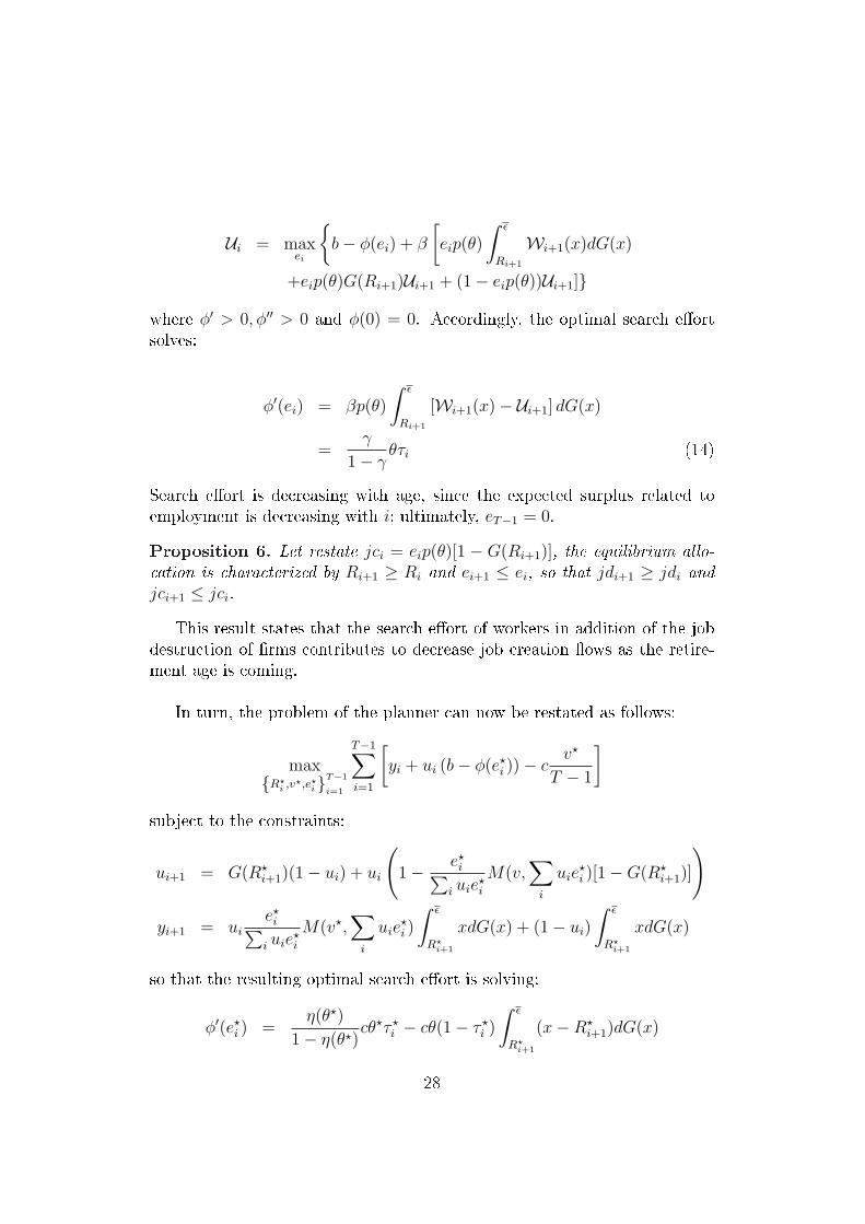
Figure 2: Age-dynamics of the employment rate: an illustration
20 30 40 50 6040
50
60
70
80
90
100Employment rate by age group
Age group
Em
ploy
men
t rat
e in
%
BelCanGerDenSpaFinFraUKItaJapSweUSmodel
Annual calibration: i = 1 refers to 16 years old workers with u1 = 1. G(ε) = ε, ∀ε ∈ [0, 1],p(θ) = Γθψ with an intermediate value T = 63, and β = .96, b = .43, ψ = γ = .6 fromconventional external informations. Γ = 1.15 and c = .78 consistent with 30-40 years oldaverage employment rate of 90%, and 1% ratio of recruiting costs to average output.
2.4.2 The age-dynamics of the employment rateThe age pro�le of hirings and �rings has been recursively determined fromterminal conditions. On the other hand, the age pro�le of unemployment ui
(or employment ni = 1 − ui) depends on the arbitrary initial condition u1.This explains why it is ambiguous:
ui ≷ G(Ri+1)
[1− p(θ)]G(Ri+1) + p(θ)⇒ ni+1 ≷ ni ∀i
Property 3. For u1 = 1, there exists a threshold age T so that ni ≥ni−1 ∀i ≤ T and ni ≤ ni−1 ∀i ≥ T .
13

Proof. See Appendix C.1.
In the case where all the new entrants are unemployed, high vacancyrates and low �ring rates at the beginning of the working life cycle make theemployment rate increasing with age until the age T . Until this threshold age,this increase in employment rate is simply the result of a queue phenomenon.From T on, the employment rate evolution by age mimics the age pro�le of�rings and hirings. The overall age-dynamics of employment is thus hump-shaped, as found in OECD data (see Figure 1). The �gure 2 put furtheremphasis on this point by providing an illustrative simulation of the modelfor a standard calibration. It must be emphasized that the model is ableto generate large variations of employment rates over the life cycle. Theemployment rate increases slowly and reaches its maximum around 40 yearsold as in most OECD countries. This illustrates the queue phenomenon inthe model which mainly depends on the hiring process. After these ages,the coming retirement age reverses the pro�le of the employment rate as theresult of the increase of the �rings at the end of the working life. One again,this pattern seems consistent with the data and reinsures us that this modelcould be also well-suited for quantitative analysis.
2.4.3 The Age Pro�le of WagesSince the seminal empirical work of Mincer [1962], it is well-known that thewage increases with age and declines at the end of the life cycle. This stylizedfact can be explained in our model simply by including general human capitalaccumulation so that: hi+1 = (1 + µ)hi where the productivity of the job isnow given by hiε which counteracts the negative impact of shorter horizonon wages, according to the value of the growth rate µ ≥ 0. Assuming thatbi ≡ bhi, it is straightforward to see that the shape of job creations and jobdestructions is not altered by this assumption, since in such a case we wouldhave:
Ri = b− β(1 + µ)[1− γp(θ)]
∫ ε
Ri+1
[1−G(x)]dx
so that Ri+1 ≥ Ri ∀i. However, it is obvious that the level of job creationsand job destructions depends on the growth rate µ.Property 4. The lowest wage paid to employed workers is strictly increasingwith age, that is wi+1(Ri+1) > wi(Ri), ∀i.Proof. See Appendix C.2.
The property 4 emphasizes that there exists a composition e�ect on wages:at the end of the life cycle, �rms hoard their workers less (the reservation
14

productivity increases with the age of the worker, Ri+1 ≥ Ri), so that onlythe more productive remain at work. This might lead the average wage toincrease with age even in the absence of human capital accumulation.
2.4.4 Distance from retirement instead of ageAn important dimension of the model is the retirement age. Only the dis-tance between the current age and the retirement age matters according to ahorizon e�ect. On the contrary, the biological age does not matter in itself.
Property 5. For two retirement ages, T and T + N , we have RT−1−i =RT+N−1−i, so that jcT−1−i = jcT+N−1−i, and jdT−1−i = jdT+N−1−i ∀i.Proof. Property 2 emphasizes that for all T we have the same terminal con-dition: for two retirement ages, T and T + N , RT−1 = RT+N−1 = b. Then,from backward induction, it comes that RT−1−i = RT+N−1−i ∀i.
Figure 3: Employment rates from age 30 to 64 for OECD Countries
1 2 3 4 5 6 7 8 9 10 110
10
20
30
40
50
60
70
80
90
100
empl
oym
ent r
ate
Jap
Swe US
UK Can Spa
Ger Ita Net Fra
Bel
Ranking of e�ective retirement age(from the highest to the lowest)
Source: OECD data for 1995 (authors' calculation). In each country, each barrefers to employment rates of the age groups : 30 - 49 (�rst bar on the left), 50 -
54, 55 - 59 and 60 - 64 (last bar on the right)
15
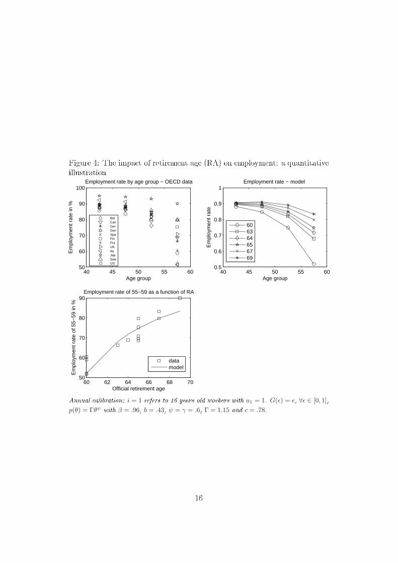
Figure 4: The impact of retirement age (RA) on employment: a quantitativeillustration
40 45 50 55 6050
60
70
80
90
100Employment rate by age group − OECD data
Age group
Em
ploy
men
t rat
e in
%
BelCanGerDenSpaFinFraUKItaJapSweUS
40 45 50 55 600.5
0.6
0.7
0.8
0.9
1Employment rate − model
Age group
Em
ploy
men
t rat
e
606364656769
60 62 64 66 68 7050
60
70
80
90Employment rate of 55−59 as a function of RA
Official retirement age
Em
ploy
men
t rat
e of
55−
59 in
%
datamodel
Annual calibration: i = 1 refers to 16 years old workers with u1 = 1. G(ε) = ε, ∀ε ∈ [0, 1],p(θ) = Γθψ with β = .96, b = .43, ψ = γ = .6, Γ = 1.15 and c = .78.
16

This may explain why countries experience a drop in their employmentrate before the normal retirement age. Figure 3 shows that the fall in theemployment rate of older worker is steeper when the retirement age getscloser, whatever the country considered. Two country groups emerged veryclearly in the mid-nineties: those with high employment rates for workersaged 55-59 (Canada, Great Britain, Japan, the United States and Sweden)and those which already experienced a huge decrease in employment rates atthese ages, around 25 points with respect to the 50-54 age group (Belgium,France, Italy and the Netherlands). As documented by Gruber and Wise[1999], the second group of countries is characterized by an e�ective retire-ment age of 60 (versus 65 in the �rst group). There is no reason to believethat these countries are more sensitive to the ongoing technological progress;they just display a lower retirement age.
Face to this huge decline in the employment rate just before the retirementrate, is our streamlined model able to generate quantitatively such outcomesfor a standard calibration? It is not say that the horizon e�ect is enoughto explain this decline alone. We aim to show that this e�ect has strongpredictive power, and is not only a theoretical curiosity. The numericalexperiment reproduced in Figure 4 put emphasis on this point. In panel A,OECD data show the decreasing shape of the employment rate by age for12 countries. These 12 countries are characterized by 6 o�cial retirementages (RA): 60, 63, 64, 65, 67 and 69. By simulating the model for these6 retirement ages, panel B gives an illustration of the property 5: startingfrom a similar level for the workers of age 45, the employment rates di�ersby a large amount 10 years later. It is less than 60% for country with aretirement age at 60, and more 85% for a retirement age at 69. It illustratesthe large elasticity of the employment rate to the retirement age in our model.It can be noticed that the employment rate for the 50-54 age group whenthe retirement age is 60 is equivalent to the employment rate of the 55-60age group in a country with a retirement age at 65. Finally, Panel C showsthat the magnitude of this horizon e�ect is in accordance with the observedheterogeneity of the employment rates in the 55-59 age group.
3 E�ciency and Labor Market Policy in a Life-Cycle Setting
The previous section showed that job separations (creations) occur more(less) at the end of the working life in our theoretical life-cycle setting. Thisresult seems consistent with facts as it has been documented by OECD [2006].
17
This feature is sometimes interpreted as a discrimination against older work-ers, whereas our analysis shows that there exists rational arguments whichpush �rms to di�erentiate their hiring and �ring policies between workerages. However, it remains to show that this behavior is not at odds withthe social optimality. Traditionally, the equilibrium unemployment frame-work is known as generating congestion e�ects which take the decentralizedequilibrium away from the e�cient allocation. However, when the elastic-ity relative to vacancies in the matching function is equal to the bargainingpower of �rms (Hosios condition), the social optimality can be reached. Doesthis result still hold when life-cycle features are considered? The existenceof a speci�c externality, namely an intergenerational externality, could leadto reconsider this result obtained in an in�nite horizon. In this case, speci�cpolicies, in particular designed by age, should be implemented to restore thesocial optimality.
First, we show that the Hosios condition breaks down in a life cycle set-ting. Secondly, we propose age-designed policies to deal with the intergener-ational externality in the search process.
3.1 Intergenerational Externality and the E�cient Al-location
We derive the optimal allocation by maximizing the steady-state output withrespect to labor market tightness θ? and reservation productivity for each age,R?
i . Accordingly, the comparison of the optimal solution with the equilibriumone will be done by considering the case β → 1.
The problem of the planner is stated as follows:
max{R?
i}T−1
i=1,θ?
T−1∑i=1
[yi + bui − cθ?
∑T−1i=1 ui
T − 1
]
subject to the unemployment dynamics and the output equation respectively:
ui+1 = G(R?i+1)(1− ui) + ui
(1− p(θ?)[1−G(R?
i+1)])
(11)
yi+1 = uip(θ?)
∫ ε
R?i+1
xdG(x) + (1− ui)
∫ ε
R?i+1
xdG(x) (12)
Proposition 2. Let η(θ?) = 1− θ?p′(θ?)p(θ?)
, the maximum value of steady-stateoutput is reached when θ? and {R?
i }T−1i=2 solve:
18

c
q(θ?)= [1− η(θ?)]
T−1∑i=1
ui
u
(∫ ε
R?i+1
[1−G(x)]dx
)
R?i = b− [1− p(θ?)]
∫ ε
R?i+1
[1−G(x)]dx
−[1− η(θ?)]p(θ?)T−1∑i=1
ui
u
(∫ ε
R?i+1
[1−G(x)]dx
)
Proof. See appendix C.3.
Property 6. The e�cient allocation is characterized by R?i+1 ≥ R?
i , so thatjd?
i+1 ≥ jd?i and jc?
i+1 ≤ jc?i .
Proof. Straightforward since 0 < [1 − p(θ?)] < 1 and by noticing that [1 −η(θ?)]p(θ?)
∑T−1i=1
ui
u
(∫ ε
R?i+1
[1−G(x)]dx)
is not age-dependent, that is onecan examine the age-dynamics of Ri by de�ning
b ≡ b− [1− η(θ?)]p(θ?)T−1∑i=1
ui
u
(∫ ε
R?i+1
[1−G(x)]
)dx.
This proposition emphasizes that higher (lower) job destruction (creation)rates for older workers is not only an equilibrium outcome but also an e�cientage-pattern of labor market �ows. Because of their shorter horizon, olderworkers must be more �red and less hired. However, this does not imply thatthe equilibrium level of job �ows is consistent with the e�cient allocation.
Proposition 3. The Hosios condition, η(θ?) = γ, no longer achieves e�-ciency in our life cycle setting.
Proof. Straightforward by comparing the expression of R?i in proposition 2
and Ri in property 2.
To see the rationale for this result, it is more convenient to restate thede�nition of the e�cient productivity threshold as follows:
R?i +
∫ ε
R?i+1
[1−G(x)]dx = b +η(θ?)
1− η(θ?)cθ?τ ?
i + cθ?(τ ?i − 1)
19
where τ ?i is de�ned as previously:
τ ?i ≡
∫ ε
R?i+1
[1−G(x)]dx
∑T−1i=1
(u?
i
u?
∫ ε
R?i+1
[1−G(x)]dx)
By comparison to the equilibrium condition (10), and contrary to Pis-sarides [2000], it is obvious that the Hosios condition γ = η(θ?) no longerachieves e�ciency in our framework because the equilibrium is no longersymmetric, that is τi 6= 1. The left-hand side of (13) represents the expectedpro�t from the marginal job occupied by a worker of age i. The right-handside corresponds to the social marginal value of an unemployed worker ofage i. It includes the leisure value b and the search value speci�c to age iunemployed workers ( η(θ?)
1−η(θ?)cθ?τ ?
i ), plus the value that this age i unemployedworkers provides through her impact on the average search value (cθ?(τ ?
i −1)).The Hosios condition γ = η(θ?) allows the private agents to internalize tradi-tional search externalities in the decentralized equilibrium. However, becausethe last term cθ?(τ ?
i −1) in the social value of unemployment does not appearin the equilibrium condition (10), the Hosios condition no longer achieves ef-�ciency. This last term re�ects that the social value of the search activityis not symmetrical: because a young (old) worker increases (decreases) theaverage search value in the economy, the social value of the young (old) un-employed worker is larger (smaller) than its market value. Hence, contraryto the �rms, the planner takes into account the impact of a particular unem-ployed worker of age i on the search process. Compared to Pissarides [2000],our life-cycle framework introduces another externality, namely an intergen-erational externality. The planner internalizes that �rings of older (younger)worker, by increasing unemployment of this age-type of workers, reduce (in-crease) the average value of vacancies. On the contrary, �rms neither takeinto account that �rings of older workers reduce the average value of a jobmatch nor that �ring of younger workers increase this average value.
Overall, this suggests that the e�cient rate of job destructions for older(younger) workers is lower (higher) than at equilibrium. The examination ofthe age-pattern of optimal labor policies will put emphasis on this result.
3.2 The Equilibrium with PoliciesThe design of age-dependent labor market policies may allow �rms to inter-nalize the intergenerational externality in their �ring policy. Traditionally,the optimality can be restored either by employment subsidies/taxes or by�ring and hiring subsidies/taxes. Following the same approach, we introduce
20
these policies, but potentially di�erentiated by age. In order to speci�callydeal with the intergenerational externality, we assume that the Hosios con-dition holds hereafter.
Let us denote ai an employment subsidy for the worker, Fi a �ring taxwhich refers to the implicit costs in mandated employment protection legisla-tion and in experience-rated unemployment insurance taxes, and Hi a hiringsubsidy. We consider a two-tier wage structure in line with Mortensen andPissarides [1999] and Pissarides [2000].
Proposition 4. A labor market equilibrium with wage bargaining and labormarket policies exists, it is characterized by:
c
q(θ)= β(1− γ)
∑i
[ui
u
(∫ ε
Ri+1+Fi+1−Hi+1
[x−Ri+1 + Hi+1 − Fi+1] dG(x)
)]
Ri = b− ai − Fi + βFi+1 − β
∫ ε
Ri+1
(x−Ri+1) dG(x)
+γβp(θ)
∫ ε
Ri+1+Fi+1−Hi+1
[x−Ri+1 + Hi+1 − Fi+1] dG(x)
ui+1 = ui [1− p(θ)(1−G(Ri+1))] + G(Ri+1)(1− ui)
with terminal condition RT−1 = b−aT−1−FT−1 and a given initial conditionu1.
Proof. See Appendix A.
3.3 The Optimal Age-Dynamics of Employment Subsi-dies
We �rst determine the employment subsidy policy suitable in the life cycleframework. We thus assume η(θ?) = γ and Fi = Hi = 0,∀i.Property 7. Let consider β → 1 and η(θ?) = γ, an optimal age-sequencefor employment subsidies, denoted {ai}T−1
i=1 solves:
ai = cθ? (1− τ ?i )
where θ?, R?i hence u?
i are de�ned by proposition 2.
Proof. Straightforward by comparing propositions 2 and 4 and recalling that∫ ε
R?i+1
[1−G(x)]dx =∫ ε
R?i+1
(x−Ri+1)dG(x).
21

Corollary 1. The optimal age-dynamics of employment subsidies is increas-ing with age, a?
i+1 > a?i ∀i ∈ [0, T − 1], and there exists a threshold age t
such that ai ≤ 0 ∀i ∈ [0, t] and ai ≥ 0 ∀i ∈ [t, T − 1].
Proof. Straightforward since from R?i+1 ≥ R?
i , we have τ ?i+1 ≤ τ ?
i and τ1 > 1,τT−1 < 1.
As the younger (older) workers exert a positive (negative) externality onhirings of older (younger) workers, there are not enough (much) destructionsof younger (older) worker jobs. This implies to subsidy more employmentof older workers, and even to tax the employment of younger workers (fori ≤ t).
3.4 Revisiting the Role of Firing taxesAlternatively to the employment tax/subsidy, it is traditional to also consider�ring taxes. This implies to also implement hiring subsidies in order to com-pensate for the e�ect of these �ring taxes on hirings. Indeed another way toreduce the unemployment of older worker is to protect their employment byintroducing age-increasing �ring taxes together with hiring subsidies. How-ever, this intuition will not be totally valid because of the particular stronge�ect of �ring taxes at the end of the working life. We �rst investigate thispoint and then turn to the optimal age-pro�le of hiring and �ring taxes.
3.4.1 On the age-di�erentiated e�ect of �ring taxesWe argue that, in a life cycle setting, there exists a non-trivial intertemporaltrade-o� related to the introduction of �ring taxes. To put emphasis on thisresult, we consider a constant tax, F , and compare its impact in our life cyclesetting versus in a MP economy (T →∞).
To that end, let �rst notice that, with T →∞, the productivity thresholdand the labor market tightness would jump on stationary values that wedenote R and θ respectively.
Property 8. If T →∞, the labor market equilibrium with �ring taxes F ischaracterized by {R, θ} solving:
22

c
q(θ)= β(1− γ)
∫ ε
R+F
(x−R− F )dG(x)
R = b− (1− β)F − βp(θ)
∫ ε
R
(x−R) dG(x)
+βγp(θ)]
∫ ε
R+F
(x−R− F ) dG(x)
Proof. Straightforward from Proposition 4 by considering Ri = Ri+1 = R.
Corollary 2. Let assume γ → 0, the labor market equilibrium is character-ized by:
0 ≥ dR
dF>
dR2
dF>
dRi
dF... >
dRT−1
dF∀i ∈ [2, T − 1]
Proof. Since, on the one hand, dRdF
= −(1− β) and on the other hand, dRi
dF=
−(1−β)+β [1−G(Ri+1]dRi+1
dFwith dRT−1
dF= −1, the proof is straightforward.
To get some intuitions on this result, let us consider the particular casewhere both β → 1 and γ → 0. It is straightforward to see that dR
dF= 0
whereas dRT−1
dF= −1 implies dRi
dF< 0 ∀i. At the end of the working cycle,
introducing a �ring tax increases the present �ring cost without any futureconsequences on the job value as the worker will be retired in the next period.On the other hand, in an in�nite horizon, the present �ring cost increases inthe same proportion as in our life-cycle model, but the job value decreases,as the �rm rationally expect the future cost of the �ring tax. In some sense,retirement allows �rms to escape from the �ring tax, leading them to morelabor hoarding for older workers. This suggests that evaluating employmentprotection in an in�nite-lived agents context underestimates the potentialpositive impact on employment. The proof of this result in the general spec-i�cation where γ > 0 is not trivial, since the larger impact of F on Ri in ourlife cycle setting accounts for a lower decrease of θ, hence of wages, than inan in�nite-horizon framework.
Nevertheless, for some parametric speci�cations, we are able to state asu�cient condition on the level of F whose implication is a decreasing age-dynamics of Ri.
23
Property 9. If F−∫ b
b−F[1−G(x)]dx ≥ ∫ ε
b[1−G(x)]dx, then RT−1 ≤ Ri+1 ≤
Ri ∀i ∈ [2, T − 1].
Proof. From the de�nition of Ri in proposition 4, by assuming Fi = F andai = Hi = 0, we have
Ri = b− (1− β)F − β
∫ ε
Ri+1
(x−Ri+1) dG(x)
+γβp(θ)
∫ ε
Ri+1+F
(x−Ri+1 − F ) dG(x)
Let de�ne Ψ(z) ≡ ∫ ε
z(x− z) dG(x)−γp(θ)
∫ ε
z+F(x− z − F ) dG(x) =
∫ ε
z[1−G(x)) dx−
γp(θ)∫ ε
z+F[1−G(x)] dx, it comes Ψ′(z) < 0, so that if RT−2 ≥ RT−1, then
Ri ≥ Ri+1 ∀i. Then,
RT−2 ≥ RT−1 = b− F ⇐⇒ F ≥∫ ε
b−F
[1−G(x)]dx− γp(θ)
∫ ε
b
[1−G(x)]dx
which implies that F ≥ ∫ ε
b−F[1−G(x)]dx is a su�cient condition for RT−2 ≥
RT−1, hence Ri ≥ Ri+1. Remaining of the proof is straightforward.
This proposition states that the employment protection can be sizeableenough at the end of the life cycle to imply that older workers face a lower riskof job destruction than younger ones. This property has strong implicationson the optimal age-dynamics of �ring taxes and hiring subsidies.
3.4.2 The optimal age-dynamics of �ring taxes and hiring subsi-dies
Let now consider ai = 0 ∀i. Firing taxes together with hiring subsidies arenow used to reach the �rst best allocation.
Property 10. Let consider β → 1 and η(θ?) = γ, an optimal age-sequencefor �ring taxes and hiring subsidies {F ?
i , H?i }T−1
i=1 solves:
F ?i+1 − F ?
i = cθ?(1− τ ?i )
H?i = F ?
i ∀i
where F ?T−1 = HT−1 = 0 and θ? and R?
i are de�ned by proposition 2.
24

Proof. Straightforward by comparing propositions 2 and 4 and recalling that∫ ε
R?i+1
[1−G(x)]dx =∫ ε
R?i+1
(x−Ri+1)dG(x).
Corollary 3. The optimal age-dynamics of �ring taxes and hiring subsidiesis hump-shaped, �rst increasing and then decreasing. Let η(θ?) = γ, F ?
i+1 >Fi ∀i < t and F ?
i+1 ≤ Fi ∀i ≥ t.
Proof. Straightforward since from R?i+1 ≥ R?
i , we have τ ?i+1 ≤ τ ?
i and τ1 > 1,τT−1 < 1.
This hump-shaped pro�le comes from two opposite forces:
• as previously stated, there are too much (not enough) destructions forolder (younger) workers, which would require, everything else beingequal, an increasing pro�le of �ring taxes and hiring subsidies.
• there is an additional force (with respect to the case of the employmentsubsidy) because the �ring tax speci�cally introduces an intertemporaltrade o�: the �rm can avoid the tax by waiting for the worker retire-ment. In words, at the end of the life cycle, a lower tax is enough toreduce �rings of older workers, because �rms have strong incentives towait for retirement of the worker. This suggests that although oldestworkers are responsible for large negative externalities on hirings ofyounger workers, it is optimal to implement a lower �ring tax at theend of the life cycle.13
4 RobustnessThis section examines robustness of our results regarding two assumptions:(i) non-age directed recruiting policies and (ii) constant search e�ort of un-employed workers.
Firstly, we show that, even though �rms could implement age-directedrecruitment policies, unemployed workers' search strategy among the set ofsub-markets would lead the equilibrium to be ex-ante non-directed.
Secondly, introducing endogenous unemployed search e�ort is found toreinforce our main results: at the equilibrium, search e�ort is decreasingwith age and the older worker search is less worthy to be encouraged as itexerts a negative congestion e�ect on the younger unemployed workers.
13Another way to understand this result would consist of considering an equilibriumdistortion which would be not age related, let say a constant unemployment bene�t denotedz. In such case, the optimal shape of �ring tax would be age decreasing, that is Fi =z + Fi+1 with FT−1 = z.
25

4.1 Age-directed SearchThe non age-directed search hypothesis appeared to play a key role in thepreceding results: it generates an intergenerational externality which was atthe heart of the market equilibrium sub-optimality. Obviously, if the modelenvironment allows to use T −1 matching technologies, one for each age, thisspeci�c externality would disappear.
Let consider age-directed recruitment policies, so that we de�ne the prob-ability of �lling a vacancy as q(θi) ≡ M(vi,ui)
vifor the �rm. In that context,
any �rm is free to open a job vacancy and engage in hiring directed to workerof age i. Let Vi be the expected value of a vacant job directed to a worker ofage i:
Vi = −c+β
[q(θi)
∫ ε
Rdi+1
Jdi+1(x)dG(x)
]+β
[q(θi)G(Rd
i+1) + (1− q(θi))]max
i{Vi}
As JdT (ε) = 0, no �rm search for workers of age T − 1, that is θT−1 = 0.
The zero-pro�t condition Vi = 0 ∀i ∈ (1, T − 2) allows us to determine thelabor market tightness for each age θi from the following equation:
c
q(θi)= β
∫ ε
Rdi+1
Jdi+1(x)dG(x) (13)
This equation implies that di�erences in expected values of jobs according tothe worker's ages have to be associated with consistent di�erences in expectedrecruitment costs. Lower expected values for older workers requires lowerexpected recruiting costs. However, this age-directed strategy will not bevalidated by unemployed workers' search among the set of sub-markets andwill not exist at the equilibrium.
Proposition 5. There is no stable equilibrium allocation with age-directedsearch.
Proof. Because there is no age-dependent ability requirement associated withthe vacancy position in our model14, an employed worker of age i 6= j or jgives rise to the same output ε into a job ex-ante age-directed toward a worker
14If in turn we would have considered that only workers of a given age can apply toage i-directed vacancies because of technological/organizational considerations, let sayjob production is hi,jε with hi,i = 1 and hi,j = 0 with j 6= i, then an age-directedsearch equilibrium would exist. Furthermore, since this equilibrium no longer featuresintergenerationnal search externalities, the Hosios condition would achieve e�ciency (proofavailable upon request).
26

of age j. The expected value of an unemployed worker of age i who searchesin an age j segment is as follows:
Udi,j = b + β
[p(θj)
(∫ ε
Rdi+1
Wdi+1,j(x)dG(x) + G(Rd
i+1)Udi+1,j
)+ (1− p(θj))Ud
i+1,j
]
= b + cθip(θj)
p(θi)+ βUd
i+1,j
where we apply the ex-post wage bargaining rule Wdi,j − Ud
i,j = γ1−γ
Ji(ε).It is then obvious that a worker of age i has incentives to search in
sub-market j instead of i, until he expects a higher probability of contact:Ud
i,j > Udi ⇐⇒ p(θj) > p(θi) ⇐⇒ θj > θi. Consequently, perfect mobility
of unemployed workers among sub-markets implies that θi = θj ∀i, j, and�nally Ud
i,j = Udi,i ∀i, j. The age-directed search strategy of �rms is then not
validated by the strategy of unemployed workers.
The condition (13), which relies on the assumption that only ui unem-ployed of workers of age i apply to i-type vacancy positions cannot hold inequilibrium. Instead, in each sub-market 1
T−1
∑T−1i=1 ui unemployed workers
apply to the vacant positions, with the same distribution of ages as in the non-directed search equilibrium. In turn, in each sub-market vj = v/[T − 1] ∀jwhere v stands for the non-directed equilibrium number of vacancies, withθ = v/(T−1)
(∑T−1
i=1 ui)/(T−1)= v
uand u are de�ned by proposition 1.
Even though age-directed search is technologically possible, the equilib-rium features ex-ante only non-directed recruiting policies.
4.2 The Role of Endogenous Unemployed Search E�ortWe propose to extend the benchmark case (with non age-directed search)to unemployment search. We analyze both the market equilibrium outcomeand its e�ciency. As workers come closer to retirement age, the return tosearch should decrease, reinforcing the decline in older worker employment.
Let ei be the endogenous search e�ort for a worker of age i, the totalnumber of hirings is now given by M(v,
∑i uiei). Then, from the perspective
of an unemployed worker the contact probability is M(v,∑
i uiei)∑i ui
ei
ewhere e is
the average search e�ort (by de�nition e ≡∑
i uiei∑i ui
). The probability forunemployed workers of age i to be employed at age i+1 is eip(θ)[1−G(Ri+1]where θ ≡ v/[
∑i uiei]. The endogenous search e�ort is derived from the
following intertemporal problem:
27
Ui = maxei
{b− φ(ei) + β
[eip(θ)
∫ ε
Ri+1
Wi+1(x)dG(x)
+eip(θ)G(Ri+1)Ui+1 + (1− eip(θ))Ui+1]}
where φ′ > 0, φ′′ > 0 and φ(0) = 0. Accordingly, the optimal search e�ortsolves:
φ′(ei) = βp(θ)
∫ ε
Ri+1
[Wi+1(x)− Ui+1] dG(x)
=γ
1− γθτi (14)
Search e�ort is decreasing with age, since the expected surplus related toemployment is decreasing with i; ultimately, eT−1 = 0.
Proposition 6. Let restate jci = eip(θ)[1 − G(Ri+1)], the equilibrium allo-cation is characterized by Ri+1 ≥ Ri and ei+1 ≤ ei, so that jdi+1 ≥ jdi andjci+1 ≤ jci.
This result states that the search e�ort of workers in addition of the jobdestruction of �rms contributes to decrease job creation �ows as the retire-ment age is coming.
In turn, the problem of the planner can now be restated as follows:
max{R?
i ,v?,e?i}T−1
i=1
T−1∑i=1
[yi + ui (b− φ(e?
i ))− cv?
T − 1
]
subject to the constraints:
ui+1 = G(R?i+1)(1− ui) + ui
(1− e?
i∑i uie?
i
M(v,∑
i
uie?i )[1−G(R?
i+1)]
)
yi+1 = uie?
i∑i uie?
i
M(v?,∑
i
uie?i )
∫ ε
R?i+1
xdG(x) + (1− ui)
∫ ε
R?i+1
xdG(x)
so that the resulting optimal search e�ort is solving:
φ′(e?i ) =
η(θ?)
1− η(θ?)cθ?τ ?
i − cθ(1− τ ?i )
∫ ε
R?i+1
(x−R?i+1)dG(x)
28

Let consider β → 1 and η(θ?) = γ. It is straightforward to see that even ifθ = θ?, ei di�ers from e?
i , and the optimal level of search e�ort for younger(older) workers have to be higher (lower) than at equilibrium. To understandthis result, let think about the optimal age pattern of a subsidy conditionalto the level of search e�ort, siei. The instantaneous utility of a unemployedworker is then b−φ(ei)+siei. Let also introduce for instance an employmentsubsidy ai as before, to achieve e�ciency, that is θ = θ?, Ri = R?
i and ei = e?i .
Property 11. Let consider β → 1 and η(θ?) = γ, an optimal age-sequencefor employment and search e�ort subsidies, denoted {a?
i , s?i }T−1
i=1 solves:
a?i = cθ?(1− τ ?
i )
s?i = −a?
i
Corollary 4. The optimal age-dynamics of employment and search e�ortsubsidies are characterized by a?
i+1 > a?i and s?
i+1 < s?i ∀i ∈ [0, T − 1],
and there exists a threshold age t such that ai ≤ 0, si ≥ 0 ∀i ∈ [0, t] andai ≥ 0, si ≤ 0 ∀i ∈ [t, T − 1].
This suggests that is not only optimal to subsidy employment of olderworkers but also to tax search e�ort of these workers. Both these resultsare consistent with the idea that unemployed older workers exert a negativeexternality on the other unemployed workers. This result gives some theoret-ical arguments to the existence of pre-retirement schemes in some Europeancountries.
5 ConclusionBecause the horizon of older workers is shorter, �rms and workers invest lessin job-search and labor-hoarding activities at the end of the life cycle: hiring(�ring) rate decreases (increases) with age. As younger workers start asunemployed, the age-dynamics of employment is hump-shaped. This resultshows that the normal retirement age is the key institution which governs theemployment rate of older workers. Countries with a low retirement age wouldalso su�er from a depressed employment rate for older workers relatively earlyin ages. This may explain why countries with a retirement age around 60 likeFrance, Belgium has also a lower employment rate for workers aged between55 and 59 than those with a retirement age of 65 like Sweden, the UnitedStates.
29
We show that this age-pro�le of job creations and job destructions is anequilibrium outcome that appears particularly robust in the life-cycle frame-work. However, age-policies are necessary to reach the optimal social outputwhen the labor market is not segmented by age. At equilibrium, there areindeed not enough (too much) job destructions for older (younger) work-ers. This feature comes from the existence of a negative e�ect exerted byunemployed older workers on the expected vacancy return which penalizesthe other unemployed workers. This is why it is optimal to subsidy the em-ployment of older workers. It does not however imply that increasing �ringtaxes during the life cycle are optimal as �ring costs are very e�cient for em-ployment protection when the retirement age is coming. Concerning laborsupply, we show that it could be optimal to discourage search e�ort of theolder workers. For a given retirement age, these results give some rationalesto age policies, such as pre-retirement, implemented in some European coun-tries.
This paper assumed that workers only di�er respectively to their distancefrom deterministic retirement. In that context, age-directed recruitment poli-cies cannot exist in equilibrium because there are any ability or organizationalage-requirement associated with jobs in the economy under study. As ourstudy gives strong importance to the non-segmented features both at thepositive and normative levels, a next issue could be to study the conditionsunder which age-segmented labor market could arise and their welfare impli-cations. However, as it was already emphasized by Kaufman and Spilerman[1982], whether or not there exists such rationales for age-segmented marketsis an empirical disputed issue.
Beyond its theoretical interest, we believe that the life-cycle unemploy-ment approach is able to deliver realistic empirical predictions. We havealready emphasized that some qualitative features such as the drop in theemployment rate at proximity of the retirement age are very well replicated.It remains to assess the quantitative performance of this approach. It cer-tainly implies to take into account other features of the life cycle. The �rstcandidate is human capital, both through initial training and experienceaccumulated during the working life. It could be interesting to study itsinterplay with labor market institutions in the line of Wasmer [2004]. Wethink that the life cycle unemployment framework provides a very promisingresearch agenda.
30

References[1] O. Blanchard and P. Portugal, What Hides behind an Unemployment
Rate: Comparing Portuguese and U. S. Labor Markets, American Eco-nomic Review, 91 (2001), 187-207
[2] J. Gruber and D. Wise, Social security around the world, NBER Con-ference Report (1999).
[3] J-O. Hairault, F. Langot, and T. Sopraseuth, The interaction betweenretirement and job search: a global approach to older workers employ-ment, IZA discussion paper, 1984 (2006).
[4] R. Hall, Employment �uctuations with equilibrium wage stickiness,American Economic Review, 95 (2005), 53-69.
[5] J. Heckman, Life cycle consumption and labor supply: An explanationof the relationship between income and consumption over the life cycle,American Economic Review, 64 (1974), 188-194.
[6] A.J. Hosios, On the e�ciency of matching and related models of searchand unemployment, Review of Economic Studies 57 (1990), 279-298.
[7] R. Hutchen, Do job opportunities decline with age, Industrial and LaborRelation Review, 42 (1988), 89-99.
[8] L. Ljungqvist and T. Sargent, The European Unemployment Experi-ence: Uncertainty and Heterogeneity, working paper (2005).
[9] L. Ljungqvist and T. Sargent, The European Unemployment Dilemma,Journal of Political Economy, 106 (1998), 514-550.
[10] T. E. MaCurdy, An empirical model of labor supply in a life-cycle set-ting, Journal of Political Economy,89 (1981), 1059-1085.
[11] J. Mincer, On-the-job training: Costs, Returns, and Some Implications,Journal of Political Economy, 70 (1962), 50-79.
[12] E. Moen, Competitive search equilibrium, Journal of Political Economy,105 (1997), 385-411.
[13] D.T. Mortensen and C. Pissarides, Job creation and job destruction inthe theory of unemployment, Review of Economic Studies, 61 (1994),397-415.
31

[14] D.T. Mortensen and C. Pissarides, New developments inmodels of search in the labor market, Handbook of LaborEconomics,North-Holland: Amsterdam (1999).
[15] OECD publishing, Live longer, work longer, Ageing and EmploymentPolicies (2006).
[16] W. Oi, Labor as a quasi-�xed factor of production, Journal of PoliticalEconomy, 70 (1962), 538-55.
[17] C. Pissarides, Equilibrium unemployment, MIT Press (2000).
[18] E. Prescott, Why do Americans work so much more than Europeans?,Quarterly Review of the Federal Reserve Bank of Minneapolis, July(2004), 2-13.
[19] R. Rogerson, Understanding Di�erences in Hours Worked, Review ofEconomic Dynamics, 9 (2006), 365-409.
[20] J. Seater, A uni�ed model of consumption, labor supply and job search,Journal of Economics Theory, 14 (1977), 349-372.
[21] R. Shimer, The cyclical behavior of equilibrium unemployment and va-cancies, Ameriacan Economic Review, 95 (2005), 25-49.
A The extended model with policyLet us denote Hi a lump sum paid to the employer when a new worker of agei is hired, Fi the �ring cost and ai the the employment subsidy for employedworkers. We follow MP by considering that the wage structure that arises asa Nash bargaining solution has two tiers. The �rst tier wage re�ects the factthat hiring subsidy is directly relevant to the decision to accept a match andthat the possibility of incurring �ring costs in the future a�ects the value theemployer places on the match. In turn, the second tier wage applies when�ring costs are directly relevant to a continuation decision.
Let the subscript i = 0 index the initial wage and the value of a job underthe terms of the two-tier contract, �rms' value functions solve:
32
V = −c + βq(θ)T−1∑i=1
[ui
u
(∫ ε
R0i+1
[J0
i+1(x) + Hi+1
]dG(x) + G(Ri+1)V
)]
+β(1− q(θ))V
J0i (ε) = ε− w0
i (ε) + β
∫ ε
Ri+1
Ji+1(x)dG(x) + βG(Ri+1) (V − Fi+1)
Ji(ε) = ε− wi(ε) + β
∫ ε
Ri+1
Ji+1(x)dG(x) + βG(Ri+1) (V − Fi+1)
The optimal productivity thresholds solve:
J0i (R0
i ) = −Hi
Ji(Ri) = −Fi
Adding the free entry condition, V = 0, it emerges that labor market tight-ness and productivity threshold are derived from the following two equations:
c
q(θ)=
T−1∑i=1
[ui
u
(∫ ε
R0i+1
[J0
i+1(x) + Hi+1
]dG(x)
)](15)
Ri = w(Ri)− Fi − β
[∫ ε
Ri+1
Ji+1(x)dG(x)−G(Ri+1)Fi+1
](16)
R0i = Ri + Fi −Hi (17)
Let us now examine the derivation of the two-tier wage structure. The lat-ter is characterized by the following two sharing rules (as a result of Nashbargaining):
W0i (ε)− Ui = γ
[J0
i (ε) + Hi +W0i (ε)− Ui
] ⇒ w0i (18)
Wi(ε)− Ui = γ [Ji(ε)− (V − Fi) +Wi(ε)− Ui] ⇒ wi(ε) (19)
so that the equations for the initial and subsequent wage bargaining are (seeappendix B.2 for details):
w0i = (1− γ)(b− ai = +γ
(ε + (1− γ)βp(θ)
∫ ε
R0i+1
(x−R0
i+1
)dG(x) + Hi − βFi+1
)
wi(ε) = (1− γ)(b− ai) + γ
(ε + (1− γ)βp(θ)
∫ ε
R0i+1
(x−R0
i+1
)dG(x) + Fi − βFi+1
)
33
which implies R0i = Ri + Fi −Hi.
Remaining of the proof is then straightforward by noticing that J ′i+1(ε) =1−γ and Ji(Ri) = −Fi implies that Ji(ε) = (1−γ)(ε−Ri)−Fi, and similarlyJ0
i (ε) = (1− γ) (ε−R0i )−Hi.
B Wage equations derivationsB.1 Wage equations (8) and (9)The sharing rule (7) can be written as:
−(1− γ)Ui = γ [Ji(ε) +Wi(ε)]−Wi(ε) (20)
From value functions (3),(5) and (6), it turns out to be that:
γ [Ji(ε) +Wi(ε)]−Wi(ε) = γε− wi(ε) + γβ
∫ ε
Ri+1
[Ji+1(x) +Wi+1(x)] dG(x)
−β
∫ ε
Ri+1
Wi+1(x)dG(x)
−(1− γ)βG(Ri+1)Ui+1 (21)
Similarly,
γβ
∫ ε
Ri+1
[Ji+1(x) +Wi+1(x)] dG(x) = γβ
∫ ε
Ri+1
[Ji+1(x) +Wi+1(x)− Ui+1] dG(x)
+γβ[1−G(Ri+1)]Ui+1
β
∫ ε
Ri+1
Wi+1(x)dG(x) = β
∫ ε
Ri+1
[Wi+1(x)− Ui+1] dG(x)
+β[1−G(Ri+1)]Ui+1
Since (7) holds for each age:
γβ
∫ ε
Ri+1
[Ji+1(x) +Wi+1(x)− Ui+1] dG(x) = β
∫ ε
Ri+1
[Wi+1(x)− Ui+1] dG(x)
so that (21) can be written as:
γ [Ji(ε) +Wi(ε)]−Wi(ε) = γε− wi(ε)− (1− γ)βUi+1 (22)
34
Incorporate this in (20) yields (8):
wi(ε) = γε + (1− γ) [Ui − βUi+1]
Then, let notice that the unemployed value (6), from the sharing rule (20)and the free entry (2), solves in equilibrium:
Ui = b + β
[p(θ)
∫ ε
Ri+1
(Wi+1(x)− Ui+1) dG(x) + Ui+1
]
= b + β
[p(θ)
γ
1− γ
∫ ε
Ri+1
Ji+1(x)dG(x) + Ui+1
]
= b +γ
1− γcθ
∫ ε
Ri+1Ji+1(x)dG(x)
∑T−1i=1
(ui
u
∫ ε
Ri+1Ji+1(x)dG(x)
) + βUi+1
= b +γ
1− γcθ
∫ ε
Ri+1[1−G(x)]dx
∑T−1i=1
(ui
u
∫ ε
Ri+1[1−G(x)]dx
) + βUi+1
where make use of p(θ)/q(θ) = θ and∫ ε
Ri+1Ji+1(x)dG(x) = (1− γ)
∫ ε
Ri+1[1−
G(x)]dx by integrating by parts. Substitute out for Ui − βUi+1 from thisexpression into wi(ε) one gets (9).
B.2 Wage Bargaining with Labor Market PolicyWe let de�ne:
W0i (ε) = w0
i (ε) + ai + β
[∫ ε
Ri+1
Wi+1(x)dG(x) + G(Ri+1)Ui+1
]
Wi(ε) = wi(ε) + ai + β
[∫ ε
Ri+1
Wi+1(x)dG(x) + G(Ri+1)Ui+1
]
The sharing rule (18) �rst can be written as:
−γHi − (1− γ)Ui = γ[J0
i (ε) +W0i (ε)
]−W0i (ε) (23)
Following the same derivation strategy as for the case without policy, we �ndthat:
γ[J0
i (ε) +W0i (ε)
]−W0i (ε) = γε− w0
i (ε)− (1− γ) (ai + βUi+1)− γβFi+1(24)
35

which implies by combining with (23):
w0i (ε) = γ (ε + Hi − βFi+1) + (1− γ) (Ui − βUi+1 − ai)
Then, from J ′0i (ε) = 1− γ and J0i (R0
i ) = −Hi, J0i (ε) = (1− γ) (ε−R0
i )−Hi
and it comes:
Ui = b + β
[p(θ)
∫ ε
R0i+1
(W0i+1(x)− Ui+1
)dG(x) + Ui+1
]
= b + β
[p(θ)
γ
1− γ
∫ ε
R0i+1
[J0
i+1(x) + Hi+1
]dG(x) + Ui+1
]
= b + γp(θ)
∫ ε
R0i+1
(x−R0
i+1
)dG(x) + βUi+1
so that we derive (20).
Similarly , from
−γFi − (1− γ)Ui = γ [Ji(ε) +Wi(ε)]−Wi(ε)
we obtain
wi(ε) = γ (ε + Fi − βFi+1) + (1− γ) (Ui − βUi+1 − ai)
and remaining of the proof to derive wi(ε) is straightforward.
C Proofs of propositions, properties and corol-laries
C.1 Proof of property 3Let us denote Ψ(Ri+1, θ) = G(Ri+1)
[1−p(θ)]G(Ri+1)+p(θ)≡ Ψi+1, so that in equilibrium
Ψi ≤ Ψi+1 < 1 from Ri+1 ≥ Ri. Accordingly, (1) implies that:
ni ≷ ni+1 ⇐⇒ ui+1 ≷ ui ⇐⇒ Ψi+1 ≷ ui
For u1 = 1, since Ψ1 < 1, it is straightforward to see that u2 < u1, hencen2 > n1. Then, from Ψi+1 ≥ Ψi > Ψ1 ∀i, there exists an age T which veri�esuT = ΨT+1, so that uT+1 ≥ uT ⇐⇒ nT+1 ≤ nT .
36

C.2 Proof of property 4Let combine wi(Ri) from (1) and substitute out
∫ ε
Ri+1[1 − G(x)]dx for Ri in
this expression yields:
wi(Ri) = γRi + (1− γ)b +γβ(1− γ)p(θ)
1− γp(θ)(b−Ri)
which implies
wi+1(Ri+1)− wi(Ri) = (Ri+1 −Ri) γ
(1− β
(1− γ)p(θ)
1− γp(θ)
)> 0
C.3 Proof of proposition 2Let us denote λi and µi the Lagrange multiplier associated with constraints(11) and (12), optimal decision rules with respect to Ri+1, θ and ui, yi arerespectively given by:
λi = µiRi+1
T−1∑i=1
c
(∑T−1i=1 ui
T − 1
)= p′(θ)
T−1∑i=1
ui
(µi
∫ ε
Ri+1
xdG(x)− λi[1−G(Ri+1)]
)
λi−1 = b−∑T−1
i=1 cθ
T − 1+ λi [1− p(θ)[1−G(Ri+1)]−G(Ri+1)]
+µi
[p(θ)
∫ ε
Ri+1
xdG(x)−∫ ε
Ri+1
xdG(x)
]
µi = 1
Substitute out for µi = 1, hence λi = Ri+1, remaining of the proof is straight-forward with the de�nition p′(θ) = [1− η(θ)]q(θ).
37