lidar signal processing techniques 9 may - diva portal470911/fulltext01.pdf · 1 introduction ......

Lidar Signal Processing Techniques

Clutter Suppression, Clustering and Tracking

THEODOR SJÖSTEDT

Master’s Degree ProjectStockholm, Sweden May 2011

XR–EE–SB 2011:010

LIDAR SIGNAL PROCESSING TECHNIQUES:

CLUTTER SUPPRESSION, CLUSTERING AND TRACKING

THEODOR SJÖSTEDT

EMBSEC AB

KTH SIGNAL PROCESSING

9 MAY 2011

Light detection and ranging (Lidar) is an object detection system, which uses the scat-tering of light, normally in the form of laser, to determine the direction, range, and oth-er properties of a distant target.

Due to the short wavelength of the laser beam, compared to traditional radio based ranging systems (radar), atmospheric phenomenon such as precipitation and fog pre-sent a major problem due to the water droplets reflectiveness at these wavelengths. Another problem encountered is that the output from the Lidar is presented as sets of two-dimensional data points, quantifying this information into discrete set of targets present a challenge. The third problem encountered in this field is that of data associa-tion, how to associate the target observations in space and time.

The data output from the Lidar was analyzed and filters where developed to counter these problems. The problem of clutter suppression was solved using heuristic methods with knowledge of the clutter distribution. The data quantization problem mandated a modified solution to an existing algorithm, while the data association (tracking) prob-lem was solved using an implementation of the Multiple Hypotheses Tracker (MHT) algorithm.

It was shown to be possible to achieve a substantial improvement to the Lidars perfor-mance by the use of smart filters. In conclusion, this thesis contributes with an interest-ing approach to the problems encountered in Lidar signal processing.

Light Detection and Ranging (Lidar) är ett objektdetektionssystem, som använder sig av spridningen eller reflektionen av ljus, vanligtvis i form av laser, för att bestämma riktningen, avstånd och andra egenskaper hos ett avlägset mål.

På grund av den korta våglängden hos laserstrålen, jämfört med traditionell radiobaserad avståndsmätning (radar), blir atmosfäriska fenomen såsom nederbörd och dimma ett stort problem på grund av vattendropparna reflektivitet vid dessa våglängder. Ett annat problem är att utdata från Lidaren normalt presenteras som en uppsättning av tvådimensionella datapunkter. Att kvantifiera denna information till en uppsättning mål är en utmaning. Det tredje problemet inom detta område är att dataassociering, hur man associerar observationer av mål i tid och rum.

Utdata från den analyserades och filter togs fram för att lösa dessa problem. Brusproblemet löstes med hjälp av heuristiska metoder och med kunskap om brusets distribution. Kvantiseringsproblemet löstes med hjälp av en modifierad implementering av en befintlig algoritm, medan data associationsproblemet (målspårning) löstes problemet med hjälp av en implementering av den så kallade MTH algoritmen.

Resultaten visade att det är möjligt att uppnå en betydande förbättring av Lidarens prestanda genom att använda smarta filter.

Sammanfattningsvis bidrar detta exjobb med en intressant lösning till problem som uppstår inom Lidarsignalbehandling.

First, I would like to thank the employees at Embsec AB in Täby for providing me with a challenging and stimulating work environment. Working on this thesis have been a very rewarding experience and has taught me many skills both within and out-side the field discussed in this thesis.

Working at Embsec has also given me a glimpse to the inside of a startup company with high ambitions and clear goals of expansion in an exciting field.

Thank you Erik Lindstein, Henrik Kjellman and Johan Strömbom.

I would like to thank Dr. Magnus Jansson at KTH Signal Processing for taking on the role as examiner of this thesis.

I would also like to give a big thank to my supervisor, PhD student Petter Wirfält for the guidance, proof reading and above all interesting discussions about this thesis.

Also, thanks to my father, Åke Sjöstedt for further proof reading this report.

Symbol Description � Wavelength [m] c Speed of light [m/s] X State vector Φ State transition matrix H Observation model matrix P Error Covariance matrix R Measurement Noise Covariance matrix Q Process Noise Covariance matrix K Kalman Gain �� Transpose of X

Abbreviation Description Laser Light amplification by stimulated emission of radiation Radar Radio direction and ranging Lidar Light direction and ranging TOF Time Of Flight SNR Signal-to-Noise Ratio NN Nearest Neighbor OFAC Online Floating Average based Clustering KF Kalman Filter LNN Local Nearest Neighbor GNN Global Nearest Neighbor PDA Probabilistic Data Association JPDA Joint Probabilistic Data Association MHT Multi-Hypotheses Tracking

1 INTRODUCTION ............................................................................................................. 1

1.1 BACKGROUND ........................................................................................................... 1 1.2 PROBLEM FORMULATION ......................................................................................... 2 1.3 PURPOSE ................................................................................................................... 4 1.4 EXPERIMENTAL SETUP .............................................................................................. 5 1.5 CHAPTER OUTLINING ................................................................................................ 6

2 THEORY OF RANGING ................................................................................................... 7

2.1 LASER BASED RANGING ............................................................................................. 8 2.1.1 RANGE ESTIMATE ................................................................................................. 8 2.1.2 ANGLE ESTIMATE .................................................................................................. 9

2.2 LIDAR VS. RADAR ..................................................................................................... 10

3 DATA CHARACTERISTICS ............................................................................................. 13

3.1 NOISE CHARACTERISTICS ........................................................................................ 13 3.2 CLUSTER CHARACTERISTICS .................................................................................... 15

4 CLUTTER SUPPRESSION ............................................................................................... 17

4.1 CLUTTER SUPPRESSION FILTER ................................................................................. 5 4.2 SNR ESTIMATE ......................................................................................................... 18 4.3 RESULTS ................................................................................................................... 18

5 CLUSTERING ................................................................................................................ 21

5.1 COMMON CLUSTERING METHODS ......................................................................... 22 5.1.1 K-MEANS CLUSTERING ....................................................................................... 22 5.1.2 MONTE CARLO EXTENDED K-MEANS ................................................................. 23 5.1.3 ONLINE FLOATING AVERAGE BASED CLUSTERING ............................................ 24

5.2 POLYGON FILTERING ............................................................................................... 26 5.3 IMPLEMENTATION .................................................................................................. 26 5.4 RESULTS ................................................................................................................... 28

6 TRACKING ................................................................................................................... 31

6.1 COMMON ESTIMATION TECHNIQUES .................................................................... 32 6.1.1 MOTION MODEL ................................................................................................. 32 6.1.2 KALMAN FILTERING ............................................................................................ 34

6.2 COMMON DATA ASSOCIATION TECHNIQUES ......................................................... 38

6.2.1 GATING ............................................................................................................... 39 6.2.2 NEAREST NEIGHBOR MATCHING ........................................................................ 41 6.2.3 PROBABILISTIC DATA ASSOCIATION ................................................................... 42 6.2.4 JOINT PROBABILISTIC DATA ASSOCIATION ........................................................ 43 6.2.5 MULTI-HYPOTHESIS TRACKING .......................................................................... 43

6.3 IMPLEMENTATION .................................................................................................. 47 6.4 RESULTS ................................................................................................................... 49

6.4.1 LNN AND MHT PERFORMANCE COMPARISON .................................................. 49 6.4.2 MONTE CARLO SIMULATIONS ............................................................................ 49 6.4.3 THE MHT TRACKING ALGORITHM WITHOUT TRACK PRUNING ......................... 54

7 DISCUSSION ................................................................................................................ 55

7.1 CONCLUSIONS ......................................................................................................... 55 7.2 FURTHER WORK ...................................................................................................... 56

8 REFERENCES ................................................................................................................ 59

FIGURE 1. AN EXAMPLE OF AN EMBSEC VFENCE S-500 ................................................. 2 FIGURE 2. REFLECTION OF EM RADIATION. .................................................................... 3 FIGURE 3. DATA QUANTIZATION PROBLEM. .................................................................. 3 FIGURE 4. DATA ASSOCIATION PROBLEM....................................................................... 4 FIGURE 5. COMMON RADAR AND LIDAR WAVELENGTHS. ............................................. 8 FIGURE 6. TIME OF FLIGHT LASER RANGER. ................................................................... 9 FIGURE 7. TWO COMMON LIDAR DESIGNS. ................................................................. 10 FIGURE 8. HEAVY SNOWFALL. ....................................................................................... 14 FIGURE 9. LIDAR SCAN. ................................................................................................. 14 FIGURE 10. DENSITY FUNCTION OF LIDAR DATA. ......................................................... 15 FIGURE 11. THE PRECIPITATION FILTER. ....................................................................... 19 FIGURE 12. THE BASIC IDEA BEHIND CLUSTERING. ...................................................... 22 FIGURE 13. ILLUSTRATION OF THE RAY CASTING ALGORITHM. ................................... 26 FIGURE 14. THE CLUSTERING TOOLBOX. ...................................................................... 27 FIGURE 15. FLOWCHART OF THE FINISHED CLUSTERING ALGORITHM ........................ 27 FIGURE 16. CLASS DIAGRAM OF THE OFAC. ................................................................. 28 FIGURE 17. POLYGON FILTERING AND CLUSTERING ALGORITHM. .............................. 29 FIGURE 18. MULTIPLE-MODEL APPROACH ESTIMATION. ............................................ 34 FIGURE 19. KALMAN FILTER FLOW CHART. .................................................................. 37 FIGURE 20. DIFFERENT GATING TECHNIQUES. ............................................................. 40 FIGURE 21. NEAREST NEIGHBOR MATCHING ............................................................... 41 FIGURE 22. NEAREST NEIGHBOR DATA ASSOCIATION PROBLEM. ............................... 42 FIGURE 23. MHT LOGIC OVERVIEW .............................................................................. 44 FIGURE 24. MHT DATA ASSOCIATION EXAMPLE. ......................................................... 44 FIGURE 25. MHT HYPOTHESIS TREE. ............................................................................. 45 FIGURE 26. COMBINATORIAL TREE MODEL FOR TRACK MERGING. ............................. 47 FIGURE 27. LNN ALGORITHM CLASS DIAGRAM. ........................................................... 48 FIGURE 28. MHT ALGORITHM CLASS DIAGRAM. .......................................................... 48 FIGURE 29. MONTE-CARLO SIMULATION TARGETS. ..................................................... 51 FIGURE 30. LNN SIMULATION RESULT. ......................................................................... 53 FIGURE 31. MHT SIMULATION RESULT. ........................................................................ 53 FIGURE 32. THE MHT ALGORITHM WITHOUT TRACK PRUNING. .................................. 54

FIGURE 33. THE EMBSEC VFENCE S-500. ...................................................... APPENDIX A FIGURE 34. THE MDL ILM T 500. ................................................................... APPENDIX B FIGURE 35. HISTOGRAM OF LIDAR DATA. .....................................................APPENDIX C FIGURE 36. 3D HISTOGRAM OF LIDAR DATA. ................................................APPENDIX C FIGURE 37. HISTOGRAM OF LIDAR DATA. .....................................................APPENDIX C

TABLE 1. COMPARISON OF DIFFERENT RANGING TECHNOLOGIES. ............................. 10 TABLE 2. KALMAN FILTER PARAMETERS. ...................................................................... 34 TABLE 3. MONTE-CARLO SIMULATION TARGET PARAMETERS. ................................... 50

Chapter 1 Introduction

1

In 2001, Embsec AB began development of a laser based Light direction and ranging system (Lidar) to be used both for perimeter control and industrial ap-plications. The Lidar is based on a laser distance meter which moves in the ver-tical axis to create an image of the environment. This type of Lidar can have many applications where long range and high accuracy is needed, such as pe-rimeter control of docks, airports and larger industrial complexes, as well as for instance finding faults with large industrial machinery.

To increase the functionality of the Lidar, this thesis was requested to develop a variety of filtering techniques to objectify the targets being tracked in a robust and efficient way.

The thesis was accepted to be published by the Signal Processing department at Royal Institute of Technology (KTH) in Stockholm, under the supervision of Magnus Jansson.

Due to trade secrets, parts of chapter 3 and 4 has been omitted from the public version of this report, and is instead presented in appendix C. This appendix can be requested from Embsec AB.

Lidar Signal Processing Techniques: Clutter Suppression, Clustering and Tracking

2

Figure 1. An example of an Embsec vFence S-500, mounted on a bridge to detect boats that are too high to safely pass under the bridge.

In my point of view, there are three fundamental problems to this application of Lidars. The first one is specific to laser based scanner technology while the last two are general problems encountered when collecting scanning data.

Atmospheric disturbances: Lasers use visible or infrared EM radiation as a carri-er of energy. The beam densities and coherency of the beam is very large. More-over the wavelengths are much smaller than can be achieved with radio systems, and range from around 10 μm to 250 nm. At such wavelengths, the waves are reflected very well from small objects. This type of reflection is called backscattering. Operating at wavelengths a factor 10,000 shorter than those used in traditional radio based radar systems; the minimal Radar Cross Section (RCS) becomes proportional to this factor (Bidigare, 2004). This is im-portant because it allows the Lidar to detect much smaller objects than conven-tional radar.


3

Figure 2. Reflection of EM radiation. Objects smaller than the wavelength of the laser pulse does not produce a strong reflection. In a), a short wave produces a strong reflection from a drop of water. In b), the longer wavelength is mostly trans-mitted, and hence does not produce a strong reflection.

Object quantization: The typical output of a scanning system is a set of angles and distances corresponding to observations made during measurement. The number of data points corresponding to a particular object may vary with dis-tance, signal quality and other factors (Amann, et al., 2001). We therefore en-counter a problem when trying to classify objects of varying size in the same scan.

Figure 3 shows us that we cannot determine whether the data collected corre-spond to one or several objects without making some assumptions of the ex-pected size of the object.

Figure 3. Data quantization problem. In a) we have a Lidar collecting data points in Cartesian coordinates. But since the laser scan can be thought of as a projection ℝ� → ℝ how can we tell if all data points correspond to one object as in b) or if they correspond to five separate objects as in c)?

λ

a) b)

λ

y

x

a)

b)

c)

Laser radar

?


4

Data association: Since a scanning laser system typically have a low frame rate, data association becomes a major problem when working on dynamical systems. E.g. how can you tell that two points at two different locations in space and time actually represent the same object? This problem increases with lower time reso-lution (scan rate). See figure 4.

Figure 4. Data association problem. Subfigure a) shows two persons, person A and person B, walking along the diagonals of the first quadrant in a Cartesian coordi-nate system with a Lidar scanning their movements at three time marks. Subfigure b) shows the output from the Lidar. At t=0 and at t=2 the scan points are easily dis-tinguishable from each other, however, this is not the case at t=1.

The purpose of this thesis is to investigate the intricacies of Lidar systems and to determine the feasibility for different signal processing techniques. It is aimed at implementing a set of solutions to the problems presented in section 1.2. It is also the aim of this thesis to increase the span of conditions under which the Li-dar can be used, as well as lowering the false alarm rate.

y

x

b)

y

x

a)

t=0

t=0

t=1

t=2

t=2

Person A

Person Bt=0

t=0

t=1

t=2

t=2Laser radar


5

The Embsec vFence S500 is a Lidar intended for object detection and classifica-tion. The maximum range is up to 500 meters. It uses a laser ranger mounted on a rotary axis. See Appendix A for a description of the vFence S500 and appen-dix B for the laser ranger used. The Lidar was mounted on a portable jig for eas-ier transport.

The implementation was made using the Python programming language with the NumPy and Matplotlib modules for linear algebra calculation and plotting re-spectively on a Debian Linux platform. The MATLAB™ IDE was also used for data analysis.


6

Chapter 2. The theory of laser based ranging will be briefly discussed in this chapter. The chapter starts with reviewing different general techniques for non-destructive ranging. Next, the Lidar will be discussed in further detail and the chapter is ended with an examination of the advantages and drawbacks of laser based ranging.

Chapter 3. To get a better view of the phenomenon encountered with this Lidar system, the data output from the Lidar was collected under various conditions and analyzed. Both the noise output from the Lidar during heavy snowfall as well as targets under low noise scenarios where analyzed and was found to hold certain characteristics.

Chapter 4. This chapter will further analyze the noise characteristics encoun-tered in section 3.1. A filter to combat this precipitation based noise as well as an estimate of the signal to noise ratio (SNR) will be developed and tested with positive results.

Chapter 5. We will in this chapter investigate common techniques for clustering data with similar characteristics together, as well as further developing a cluster-ing technique suited to be used with the scanning Lidar. Result show excellent result and this algorithm is as of today in use in commercial applications.

Chapter 6. Common techniques for target tracking will be covered in this chap-ter. An algorithm known as the multi hypothesis tracker (MHT) as well as the naïve local nearest neighbor (LNN) tracker are implemented and simulated.

Chapter 7. In this chapter, we will attempt to discuss the results obtained in this thesis and point out what went well and what was not implemented due to a lack of time. This will extend into a discussion on what could be accomplished if the work presented in this thesis where to be continued.

Chapter 2 Theory of Ranging

7

In this chapter, the theory of laser based ranging will be briefly discussed. The chapter starts with reviewing different general techniques for non-destructive ranging. Next, the Lidar will be discussed in further detail and the chapter is ended with an examination of the advantages and drawbacks of laser based rang-ing.

Non-destructive absolute distance measuring has emerged as an important con-tribution of modern science. By emitting an electromagnetic or mechanical sig-nal and then measuring the reflected or scattered return we can determine the distance to a target.

Mechanical transducers such as sonars are used only to measure distance through a compressional media such as water or air, but only at shorter distances for the latter.

Light detection and ranging (Lidar) is an object-detection system which uses the scattering of light, normally in the form of laser, to determine the direction, range, and other properties of a distant target. One of the most common ways of determining the distance to an object is the Time of Flight (TOF) method, in which a short laser pulse is emitted and the delay until the return is measured. (Cracknell, et al., 2007)

Lidar technology share many similarities to radar technology, both in the way the way the sensor data is collected, and the way the post-processing is conduct-ed. Radar literature is abundant and comprehensive; this is not the case with the Lidar.

In air and/or vacuum, most commercial distance measuring equipment operate in either the upper radio bands, 3 cm to 15 cm for radar or in the visible or near vis-ible light spectra, 400 nm – 2000 nm for Lidars, see figure 5.


8

Figure 5. Common radar and Lidar wavelengths. Note that this is not a linear scale.

A Lidar works by estimating two parameters, distance and angle. The most common ways of measuring distance using laser light is by triangulation, pulsed time-of-flight, phase shift measurement and frequency modulated continuous wave modulation (Cracknell, et al., 2007). Out of these, the second one is the most commonly used, and the one I have been using in my experiments.

The angle is commonly used estimated using a rotary encoder of some sort.

The time-of-flight (TOF) distance measurement technique is based on elemen-tary physics, but requires careful timing to be accurate. The TOF timing circuit triggers a laser pulse which is reflected and detected by the detector pre-amplifier. Since the speed of light (c) is known, distance can be calculated from the time passed from transmitting to receiving the pulse, see figure 6.


9

Figure 6. Time of Flight laser ranger. Note that the simpler laser rangers may share optics between transmitter and detector.

Radar and Lidar technology share many similarities, the primary difference be-ing that Lidars uses much shorter wavelengths of the electromagnetic spectrum, typically in the UV to IR range.

In theory it is possible to detect an object only if the size of the object is about the same or larger than the wavelength used by the sensor. Because of this, Li-dars are normally very sensitive to aerosols and particles, mist and precipitation being a major issue.

By connecting the laser ranger to a motor drive unit with a high resolution en-coder, or reflecting the laser beam with a rotating mirror, both a distance and angle can be estimated simultaneously, see figure 7.

The laser can be mounted directly, or via some sort of transmission, to the mo-tor. This mirror less system have the advantage of being very simple but accu-rate.

The laser can also be stationary, while a mirror is mounted on the motor to move the laser beam. The advantage of the mirrored system is that the inertia of the mirror is much lower than that of the laser, which allows for higher scanning speed. The drawbacks include alignment issues and refraction losses.

Detector & Pre-amplifier

Amplifier with automatic gain

control

Transmitter (laser unit)

Time measurment

circut

Start pulse

Stop pulse

Distance estimate

ObjectOptics


10

Figure 7. Two common Lidar designs. Subfigure a) shows a system where the laser ranger is mounted directly on the motor shaft. In subfigure b), the laser is stationary while a mirror is mounted on the motor instead.

Light based ranging have a few major advantages and drawbacks to radio based ranging:

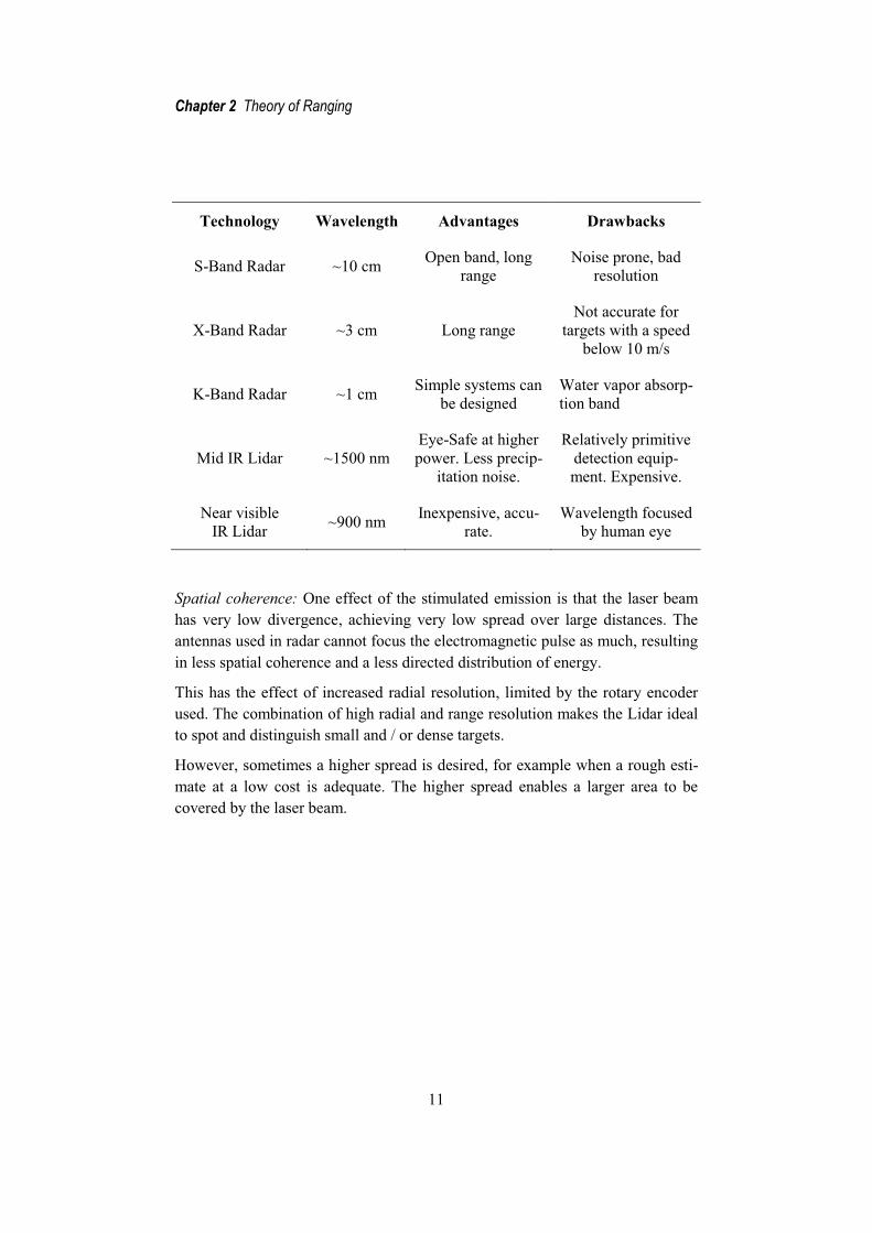
Resolution: Table 1 shows us that the wavelength of visible or near-visible light is a factor 30,000 smaller than that of the radio waves used in commercial X-band radars; this will allow for much higher spatial resolution. This is why a Li-dar with an added tilt axis can be used for 3D scanning of for example buildings, bridges and rock formations. This cannot be done with a radar system.

However, the higher spatial resolution is also one of the major drawbacks, since the shorter wavelengths allows for reflections from much smaller objects, such as water vapor, hence the laser have a hard time “seeing through” fog, smoke, heavy rain and snowfall.

Another drawback connected with the higher frequencies is that they are more quickly absorbed by the atmosphere, hence lowering the range.

Table 1. Comparison of different ranging technologies.

MotorMirror

Laser /

detector

Laser / detector

Motor

Encoder

Encoder

a) b)


11

Technology Wavelength Advantages Drawbacks

S-Band Radar ~10 cm Open band, long range

Noise prone, bad resolution

X-Band Radar ~3 cm Long range Not accurate for

targets with a speed below 10 m/s

K-Band Radar ~1 cm Simple systems can be designed

Water vapor absorp-tion band

Mid IR Lidar ~1500 nm Eye-Safe at higher power. Less precip-

itation noise.

Relatively primitive detection equip-ment. Expensive.

Near visible IR Lidar ~900 nm Inexpensive, accu-

rate. Wavelength focused

by human eye

Spatial coherence: One effect of the stimulated emission is that the laser beam has very low divergence, achieving very low spread over large distances. The antennas used in radar cannot focus the electromagnetic pulse as much, resulting in less spatial coherence and a less directed distribution of energy.

This has the effect of increased radial resolution, limited by the rotary encoder used. The combination of high radial and range resolution makes the Lidar ideal to spot and distinguish small and / or dense targets.

However, sometimes a higher spread is desired, for example when a rough esti-mate at a low cost is adequate. The higher spread enables a larger area to be covered by the laser beam.


12

Chapter 3 Data Characteristics

13

To get a better view of the phenomenon encountered with this Lidar system, the data output from the Lidar was collected under various conditions and analyzed. Both the noise output from the Lidar during heavy snowfall as well as targets under low noise scenarios where analyzed and was found to hold certain charac-teristics.

Due to trade secrets, parts of this chapter has been omitted from the public ver-sion of this report, and is instead presented in appendix C. This appendix can be requested from Embsec AB.

As discussed in section 3.1, precipitation can be a major source of noise in Lidar systems for outdoor use. Figure 8 - 36 shows measurements made during heavy snowfall. The scan rate was approximately 0.2 � and data was collected under ca two hours of varied snowfall.


14

Figure 8. Heavy snowfall. Photo from the view of the laser scanner. The location is the E18 freeway located in Täby, north of Stockholm.

Figure 9. Lidar scan. This is an accumulated scan during heavy snowfall.

Note that some content in this section is available in appendix C, due to trade secrets.

Chapter 3 Data Characteristics

15

Since we want to be able to use the Lidar in a varied selection of weather scenar-ios without severely limiting the performance, new types of filters have to be developed.

Figure 10. Density function of Lidar data. Subfigure a shows data points outputted from the Lidar and b shows a density estimate of these data points.

Looking at figure 10 we see that the points are grouped in clusters resembling a bivariate normal distribution, which is predicted by the Central Limit Theorem, which states that the mean of a sufficiently large number of independent random variables, each with finite mean and variance, will be approximately normally distributed (Rice, 1995).

We can use this information when developing filters to group (cluster) data points.


16

Chapter 4 Clutter Suppression

17

This chapter will further analyze the noise characteristics encountered in section 3.1 and appendix C. A filter to combat this precipitation based noise as well as an estimate of the signal to noise ratio (SNR) will be developed and tested with positive results.

Due to trade secrets, parts of this chapter has been omitted from the public ver-sion of this report, and is instead presented in appendix C. This appendix can be requested from Embsec AB.

In figure 9 and 35 - 36 in Appendix C, we see that heavy precipitation such as snowfall could be a major source of problems. We cannot completely get around this fact, but we can use our knowledge of the noise characteristics to gain a bet-ter estimate of the interesting data.

Radar clutter is commonly modeled as a Rayleigh, Log-Normal or Weibull dis-tribution (Schleher, 1976). In figure 37 in appendix C we can see a fit of our ac-cumulated data presented in figure 35 to these distributions.

Due to trade secrets, this section has been omitted from the public version of this report, and is instead presented in appendix C. This appendix can be requested from Embsec AB.


18

The Signal-to-noise Ratio (SNR) can be estimated by using the properties of the laser distance meter presented in appendix B. It was shown that during “bad” conditions, such as fog and heavy rain and snow, the probability of the meas-urement failing was considerably higher. This failed measurement is outputted as a distance way beyond the sensor range, and is hence easy to distinguish from successful measurements.

A heuristic approach to this SNR estimate is the following expression,

� ��, �� = 20 log �∑ ��∑ �� = 20 log � ∑ �∑ �� − 1�, (1)

where �, �� and �� are the total number of measurements, the number of suc-cessful measurements and the number of failed measurements in the measure-ment series respectively. This way of estimating SNR might be viewed as slight-ly ad-hoc, but since the laser ranger is largely a black box system, because of trade secrets; the details of the internal workings of the system are unknown.

The filter described in section 0 was applied to the data series collected during heavy snow-fall, which was presented in section 3.1. This test1 is illustrated in figure 11.

The algorithm was very successful in filtering out noise induced by falling snow. Only smaller targets sometime gave a false positive return (classified as noise) from the clutter filter due to the relatively few number of data points correspond-ing to this target.

1 The full test series in animation-form is available online at http://www.youtube.com/watch?v=AyVGA7-8z9I, as of 24 Jan 2011.

Chapter 4 Clutter Suppression

19

Figure 11. The precipitation filter. Four frames of the clutter suppression filter de-rived in section 0 with the data series from section 3.1. Note that the data was clus-tered before filtered, green crosses indicate that the measurement originated from a “true” source, red squares from clutter. The stationary target present in subfigure a), b) and c) is a lamp-post on the highway. The positive reading at (x,y) = (-7,48) in a) and (x,y) = (-4,36) are vehicles passing on the highway, the second one probably a bus or truck due to its size. In d), the snow is too heavy to observe any-thing other than noise.


20

Chapter 5 Clustering

21

We will in this chapter investigate common techniques for clustering data with similar characteristics together, as well as further developing a clustering tech-nique suited to be used with the scanning Lidar. Result show excellent result and this algorithm is as of today in use in commercial applications.

Clustering is the process of dividing data with similar properties into discrete groups. The aim is to take advantage of natural properties in the data such as the grouping tendency towards a multi variant normal distribution discussed in sec-tion 3.2. The greater the homogeneity of the data within a cluster, the greater is the chance of successful clustering. Figure 12 shows the basic idea behind clus-tering. Note that the clustering techniques presented in this chapter is applicable to other type of sensor systems that present its data in a similar data form, for example radar. It is not specific to the Lidar system.

The advantages of clustering data are many. These include:

Complexity reduction: You can reduce the number of parameters to describe the data. For example, a set of 1,000 points in the Cartesian coordinate system may only need ten clusters to describe its fundamental outlook.

Intuitiveness: The human eye have no problem spotting clusters in natural envi-ronments. For instance, we can easily distinguish a flock of birds from another even though the flock is made up of hundreds of individuals.


22

Figure 12. The basic idea behind clustering. a) shows the original 2D points. In b), two clusters where created, while in c) four clusters where created. Again, this shows the need for assumptions about the size of the objects being clustered.

This section will briefly cover a few common partitional clustering techniques. A partitional algorithm seeks to partition a given space into discrete clusters. The interested reader is referred to (Tan, et al., 2005) for a more comprehensive review of these techniques.

k-Means Clustering is a recursive, prototype based clustering technique. Proto-type based means that the algorithm starts with a rough estimation of the clusters positions. This algorithm seeks to partition n data points into k clusters. The number of clusters must be known in beforehand, which can be an advantage or a drawback, depending on the application. Another potential danger is that the recursive algorithm easily gets stuck in a local minima, due to the randomly se-lected initial clusters.

The algorithm works by randomly selecting k data points as initial means. The k clusters are then created by assigning each data point to its closest mean. The centroids of the newly formed clusters become the new means. This is repeated until convergence.

Formally, we seek to minimize the square error described below (2).

a) Original points. b) Two clusters. c) Four clusters


23

��min� � � �� − �!�"�#∈�%

&!'( (2)

Where the outer sum describes the loop through the k clusters, the inner sum the loop through the set (S) of data points (x) in the respective cluster. ) is the mean of each cluster. The centroid is the arithmetic mean of the cluster.

Monte Carlo extended k-Means is a variant of k-Means which seeks to lessen the algorithms tendency to get stuck in local minima.

The Monte Carlo algorithm works by running m test series with the k-Means algorithm, generating m different cluster sets. The cluster set with the lowest cost is then selected as the final cluster set.

The cost function

*+ = 1� � -(�!)4!'( (3)

estimates the mean variance of the cluster set. The theory being that a “good” cluster is more compact than a “bad” cluster and hence have lower variance.


24

The clustering techniques described in the previous section show a major draw-back; they all use batch type updates, which makes them computationally inef-fective for our application. The clusters can only be calculated after the sweep of the laser scanner is finished. k-Means clustering also have the added drawback of requiring the user to know the number of clusters to be formed in beforehand. We could develop an adaptive algorithm to try different numbers of clusters, but a better idea would be to develop a lean algorithm that dynamically creates new clusters when necessary while the scanner is scanning.

Basing our online algorithm on the k-Means algorithm we first have to adapt the way a point is assigned to a cluster. The simplest and most naïve approach of doing this is to use the Nearest Neighbor (NN) technique. If a data point is with-in a radius �"!4 to any cluster mean, the point will be assigned to the closest cluster. If not, a new cluster will be formed.

Proceeding from this, a new point 5! will be assigned to a cluster with index:

arg� 5!,� = 6argmin78�8& �)� − 5!� 9: ∀ )�: �)� − 5!� ≤ �"!4? + 1 ABℎD�E9FD (4)

That is, if a point lies within �"!4 of any of the ? cluster mean, the cluster index j of the new point with index i will be that of the closest cluster. If no cluster lies within �"!4 range, the point will be given the index ? + 1, hence creating a new cluster.

In the original k-Means algorithm, updates of the cluster means are done after the scan is finished and the means are extracted by calculating the centroid of the data points in the cluster. This is a very poor way of calculating the mean in an online algorithm. Instead, the updated position of the cluster means can be calcu-lated recursively as by the following derivation:

The arithmetic mean of 5̅ of � datapoints at time step ? is defined as


25

5̅(?) = 1� � 5!4! . (5)

With the corresponding mean at time step ? − 1

5̅(? − 1) = 1� − 1 � 5!4H(

! . (6)

By extracting the n:th term from the sum in (5) we get

5̅(?) = 1� � 5! +4H(!

1� 54. (7)

By expanding the first term in (7) with � − 1 and we get

5̅(?) = � − 1� 1� − 1 � 5! +4H(!

1� 54. (8)

We can now eliminate the computationally costly sum by the fact that (6) is em-bedded in (8). All this results in

5̅(?) = 1� ((� − 1)5̅(? − 1) + 54). (9)

We have now developed a complete, computationally effective online clustering algorithm. One major advantage of this algorithm is that it only needs one varia-ble for tuning, �"!4. This allows for simple and intuitive tuning, see clustering result in figure 17.

As a last point on this subject, we can chose also to delete small clusters under a certain threshold value to suppress some clutter, again depending on the applica-tion.


26

By clustering all data points that enter the scanner system, we will get a lot of clusters consisting of the background environment and other unwanted areas. A practical way of raw-filtering the data is to define a polygon, the Perimeter Pol-ygon, inside which, data is considered interesting.

One popular method of determining whether a point lies within a polygon or not is the Ray Casting algorithm. This algorithm works by measuring how many times an imagined line with its origin outside the bounding box of the polygon intersects the polygons edges. If the number of edges crossed along this line is odd, the point lies within the polygon. If even, the point lies outside the polygon. This observation may be proven mathematically by using the Jordan Curve The-orem (Haines, 1994). See figure 13.

Figure 13. Illustration of the Ray Casting algorithm. An imagined line with its origin outside the bounding box of the polygon is casted towards the point of inter-est.

The clustering algorithm was implemented in Python. It is a simple, yet power-ful algorithm with only three classes and around 100 rows of code. See figure 15 for a full flowchart of the algorithm, including the Polygon filter discussed in section 5.2 and figure 16 for a class diagram of this algorithm which illustrates the algorithms classes, methods and variables.

Crossed line

Non-crossed line

Casted line

x

y

Point

Origin


27

A Graphical User Interface (GUI) was developed for the purpose of testing the clustering algorithm with different datasets and different settings. This GUI was named “Clustering Toolbox”, and was implemented using the wxPython module in the Python programming language. The Clustering Toolbox also implemented the Polygon filtering algorithm, and allowed for free-form creation of filter pol-ygons, see figure 14.

Figure 14. The Clustering Toolbox. This GUI was developed to test different data-sets and settings. Here, a free-hand polygon has been created (light green) and points filtered out (dark green). See figure 17 for an example of the effect different �"!4 has on this data.

Figure 15. Flowchart of the finished clustering algorithm Note that this figure in-cludes the polygon filtering technique covered in section 5.2 .

Within Peremiter Polygon?

Closest cluster centroid within

rmin?

Start new cluster

Join point to the closeset

clusterno yes

Centroid for this cluster is

the new point.

Update centroid for this

cluster.

Scan finished?

yes

Clustersize below minimum?

no

yes

Discard point / cluster

no

yes

New data point?no yes

no


28

Figure 16. Class diagram of the OFAC. The Online Floating Average based Clus-tering algorithm with relations, methods and variables.

The clustering algorithm was evaluated on real data collected from an oblong room. It is the same raw data visible in figure 14. The data was evaluated using the Clustering Toolbox described in the previous section with an increase in the clustering parameter rIJK, spanning from 1 m to 8 m, see figure 17.

The clustering algorithm showed excellent results for this type of high-SNR type data. In situations with where the SNR is lower due to high noise presence, clut-ter will also be clustered, which is a problem. However, the clutter suppression filter derived in section 0 can be implemented to help this out.

+centroid : Point+label : int+points : list

Cluster+reset()+newCluster()+updateCentroid()+addPointToCluster()+closestCentroid()+addPoint()

+r_min : float+labels : list+clusters : list

Clusters+x : float+y : float

Point


29

Figure 17. Polygon filtering and clustering algorithm. Here applied to the data visible in figure 14 using the Clustering Toolbox. In a) to d) we have an increase in the clustering parameter �"!4 , spanning from 1 m to 8 m. The coordinates in the la-bels mark the clusters mean.


30

Chapter 6 Tracking

31

This chapter will cover common techniques for target tracking. An algorithm known as the multi hypothesis tracker (MHT) as well as the naïve local nearest neighbor (LNN) tracker are implemented and simulated.

In the context of this thesis, tracking is the process of estimating one or more objects true motion through time and space by the means of some observations. The goal is for the sensor to gather readings of the environment containing one or more potential targets of interest and to partition the sensor data into tracks that are produced by the same target. An intrinsic benefit of tracking is that quantities such as target velocity, acceleration and future predicted location, can be estimated. Note that the tracking techniques presented in this chapter is appli-cable to other type of sensor systems that present its data in a similar data form, for example radar. They are not specific to the Lidar system, in fact the tech-niques presented in the references literature of this chapter where first developed for radar systems.

There are fundamental differences to a single-target tracking system (STT) and multiple target tracking systems (MTT). A common way of implementing a STT system on a scanning radar is to attempt to align the sensor head with the target, thus allowing the tracking algorithm to take mechanical control of the movement of the radar.

For many application, tracking only one object is enough. But there is one mayor concern - even if we were only interested in tracking one target, the pres-ence of another target might render the STT techniques useless. That is, the STT techniques requires one unique, strong target.

For an example that highlights this issue, see figure 4 in section 1.2. In this illus-tration two persons are walking along the diagonals of the first quadrant of a Cartesian coordinate system. If you are only interested in tracking person A, why would you go through the extra effort of also tracking person B? This is necessary because both person A and B have the same expected return from the scanning Lidar. At time step t=1, it is not possible to tell them apart at all, hence loosing track of person A is a real possibility.


32

Unfortunately, the extension from STT to MTT often requires complex data as-sociation techniques for robust operations.

For an interesting presentation of real-world applications of tracking algorithms described in this chapter, see page 96-98 of (Bar-Shalom, et al., 2009).

A basic concept in estimation theory is the so called motion model. This is a model on how the tracked target is expected to behave. This motion model can then be used to predict the future state of the target. This prediction is at best a rough approximation, especially when trying to track e.g. humans or machines operated by humans, which can be very unpredictable.

By making the two basic assumptions that 1) The current state is only dependent on the previous state, i.e. only the immediate past matters and 2) the current measurement is conditionally independent from all other measurements, the es-timation problem takes the form of a discrete time Markov process.

One of the simplest motion models is one where we assume the target to have a constant velocity. This is a linear model where the updated position is assumed to have the same velocity as the estimated velocity in the previous time step. A white noise term E(?) is often also incorporated into this simple model, thus allowing the velocity to change by means of an induced acceleration term, all in a stochastic manner.

In this case if we have the state � = (5, L, 5,̇ L̇)�, where x and y is the position and 5̇ and L̇ is the velocity of a target. If the target state has a zero-mean white Gaussian noise N(?) with the known covariance O, this results in the state space equation:

�(? + 1) = Φ�(?) + N(?) (10)

With the state transition matrix,

Chapter 6 Tracking

33

Φ = P1 0 Q 00 1 0 Q0 0 1 00 0 0 1R, (11)

where T is the sampling time. We can easily extend this model into the so-called constant acceleration or coordinated turn model (from the constant acceleration an airplane experiences during a coordinated turn). In this case we will have the state vector � = (5, L, 5,̇ L,̇ 5̈, L̈)�, where x and y is the position, 5̇ and L̇ is the velocity and 5̈ and L̈ is the acceleration of a target. This allows us to predict the movement of a target even though it is currently turning.

The state transition matrix now looks like

Φ =⎣⎢⎢⎢⎢⎢⎡ 1 0 Q 0 Q 2W 00 1 0 Q 0 Q 2W0 0 1 0 Q 00 0 0 1 0 Q0 0 0 0 1 00 0 0 0 0 1 ⎦⎥⎥

⎥⎥⎥⎤. (12)

An estimator may use one or several motion model to drive its time update.

The Kalman filter is one of the most widely used estimators due to its relative simplicity and the fact that it’s an optimal estimator for many applications. The Kalman filter is described in some detail in section 6.1.2.

A Kalman filter with a single motion model may not always be sufficient to de-scribe the sometimes nonlinear dynamics of a maneuvering target. In the multi-ple-model approach, several models are used simultaneously, each with its own filter. The probability of each model being correct is then calculated.

The estimate with the highest probability will either be weighted the highest in a weighted average of the estimates or simply chosen as the only correct model at this instance (Bar-Shalom, et al., 1987). See figure 18 for a simplified flowchart of this filter.

A commonly used multiple model is the so called Interacting Multiple Models (IMM). This model is described in detail in (Hong, 1999)

A scenario where this could be useful is for example the human gaits, where walking and running represent two overlapping Gaussian distributions.


34

Figure 18. Multiple-model approach estimation. The filter bank holds n filters, for example the Kalman Filter.

The Kalman filter is a linear filter first proposed by Rudolf E. Kalman in his 1960 paper (Kalman, 1960) as an extension to earlier work by Norbert Wiener (Wiener, 1949).

The Kalman filter seeks to gain a better estimate of the true value by estimating the uncertainty of the predicted and observed values and weighting these to which ever have the lower uncertainty. The filter provides an efficient recursive solution of the least-squares method, i.e. it minimizes the square error.

The Kalman filter has two distinct phases, the Prediction phase and the Update phase. The prediction phase occurs every time period T, while the Update phase only occurs when a new observation is available. For easier understanding of the relations mentioned in this text, I would recommend the reader to refer to figure 19 for a flow chart of the filter functions and table 2 for a summary of the Kal-man parameters.

Table 2. Kalman filter parameters.

Measurment system

Environment

Filter n-1Filter 1 Filter n

Measurment system

Calculation of probability

Estimate

Chapter 6 Tracking

35

Symbol Name Description

5, 5[ State, state estimate. The state variable holds the current val-ues of the properties being estimated, e.g. position and velocity.

Φ Motion model or State transition matrix.

The motion model is described in detail in section 6.1.1.

� Observation An observation is a set of one or more measurements.

Observation model The observation model maps the true state space into the observed space.

\ Error covariance The covariance of the residual

� Measurement noise covar-iance

Estimate of known or unknown meas-urement noise, e.g. sensor noise.

O Process noise covariance Estimate of the “randomness” of the process, e.g. the fluctuation of velocity of a constant velocity model.

], E Measurement noise and Process noise respectively

Zero mean Gaussian white noise.

In the Prediction phase, the state 5 is estimated using only the motion model times the previous state estimate,

5[&|&H( = ^5&H(|&H( + E&, (13)

where the Gaussian, zero mean noise term E&~ (0, O) is included in this mod-el. The predicted (a priori) error covariance is also estimated with a sampling time T using the motion model and the estimate of the process noise term Q,

\&|&H( = Φ\&H(|&H(Φ� + O. (14)

When a new observation �& is present it is modeled as

�& = 5&|&H( + ]&, (15)

where ]& is also a Gaussian zero mean noise, ]_~ (0, �).


36

The Update stage tries to better the state estimated in the prediction state by the observed data. The residual and updated (a posterior) innovation covariance is calculated as

L̀& = �& − 5[&|&H( (16)

and

�& = \&|&H(� + � (17)

respectively. The a posterior state estimate and error covariance is calculated as a weighted average of the a posterior estimation and the a posterior innovation residual and covariance, using the “Kalman gain”, K, as a mixing factor.

5[&|& = 5[&|&H( + b&L̀& (18)

The Kalman gain is chosen to minimize the a posteriori covariance (19):

\&|& = (c − b&)\&|&H( (19)

One form the Kalman gain is:

b& = \&��&H( (20)

Looking at equations (19) and (20) we can see that as the measurement error covariance R approaches zero, the gain weights the a posterior residual more heavily.

limd→7 b& = H( (21)

Similarly, when the a priori error covariance (14) approaches zero, the gain weights the a posterior residual less heavily:

limef|fhj→7 b& = 0 (22)

Chapter 6 Tracking

37

The Kalman gain can be viewed as a measure how much you “trust” your meas-urements (sensor data) and dynamical model respectively. This is the main rea-son that the Kalman filter is optimal for linear models with Gaussian noise terms (Welch, et al., 2006), (Sorenson, 1970). Another practical advantage caused by this is that it can handle an extended absence of measured data, only relying on the motion model for updating.

Figure 19. Kalman filter flow chart. The filter has two distinct phases, the Predict and Update phase. The predict phased occurs every time period T, while the Update phase only occurs when a new observation is available. Note that “I” is the identity matrix.

PREDICT

UPDATE

Covariance estimate

Covariance estimate

Kalman gain

State estimate

Innovation residual Innovation covariance

1|11| ˆˆ �� kkkk xx QPP Tkkkk �� 1|11|

1|ˆ~�� kkkk xHzy RHHPS T

kkk �� 1|

11|

�� k

Tkkk SHPK

kkkkkk yKxx ~ˆˆ 1|| �� 1|| )( �� kkkkk PHKIP

State estimate


38

Data association is the process of determining which data points in an observa-tion originated from the same target. Figure 4 in section 1.2 highlights this prob-lem in a simplified figure.

The series of observations captured with the laser scanner can be seen as a linear transformation ℝ → ℝ�, time being the third dimension.

While estimation, covered in the previous section, becomes difficult in noisy environments, data association becomes very difficult.

There are three major techniques used to solve the data association problem, which are:

The Target-Oriented Approach uses information on the targets known in before-hand, such as the number of targets etc. These algorithms include the Nearest Neighborhood Matching and Probabilistic Data Association algorithms.

The Track-Oriented Approach treats each track individually and is therefore suited in noisy environments and when the number of tracks is not known in beforehand.

The Multiple Hypotheses Approach does not decide on one set of “best” tracks, but tries different combinations of data associations. Whichever set of tracks gets the best fit is presented to the user. This is generally considered the most complex data association technique, but also one of the most effective in noisy environments.

Chapter 6 Tracking

39

Gating is a technique for eliminating unlikely observation-to-track associations. Gating decreases the computational load and helps prevent incorrect associations when there are no true observations of the object, and the closest false observa-tion is far away from the predicted position. (Blackman, et al., 1999)

The most basic form of gating is the rectangular gate illustrated in figure 20 a). When the following criteria is fulfilled, the point lies within the gate:

kp5qLqs − p5"L"sk ≤ p�ts (23)

Where index m indicate a measurement point and p a predicted point. The di-mensions a and b are as shown in figure 20a.

Another very basic form of gating is the fixed radius gate illustrated in figure 20b. With this form of gate, all measurements that lie outside a pre-determined radios �"uv from the predicted position are excluded from further processing. This form of gating can easily be extended to an ellipsoidal gate, see figure 20c. The circular gating equation is given by

�5q − 5"� + �Lq − L"� ≤ �"uv , (24)

where index m indicate a measurement point and p a predicted point and the el-lipsoidal gating equation is given by

5"� + L"t ≤ 1 , (25)

where the dimensions a and b are as shown in figure 20c.

When working with a probabilistic based filter, such as the Kalman filter, we can use the innovation covariance estimate (17) as a measure of uncertainty of the estimate when gating new measurements.

One probabilistic based gating expression (Reid, 1979), is given by

L_w ��H(L_w ≤ x, (26)


40

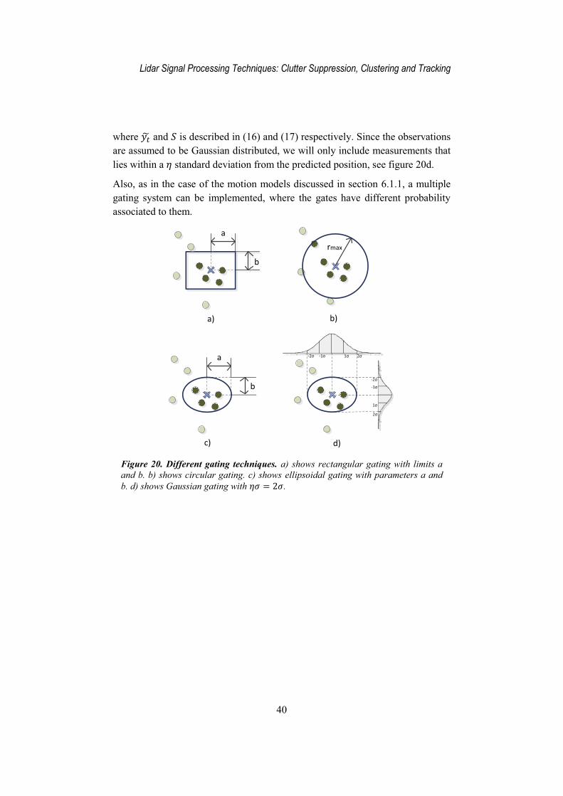
where L_w and � is described in (16) and (17) respectively. Since the observations are assumed to be Gaussian distributed, we will only include measurements that lies within a x standard deviation from the predicted position, see figure 20d.

Also, as in the case of the motion models discussed in section 6.1.1, a multiple gating system can be implemented, where the gates have different probability associated to them.

Figure 20. Different gating techniques. a) shows rectangular gating with limits a and b. b) shows circular gating. c) shows ellipsoidal gating with parameters a and b. d) shows Gaussian gating with xy = 2y.

a) b)

c) d)

a

b

a

b

rmax

-1σ -2σ 1σ 2σ

-1σ

-2σ

1σ

2σ

Chapter 6 Tracking

41

The Nearest Neighbor (NN) matching algorithm is probably the simplest and most naïve data association algorithm. The measured point that have the shortest distance to the predicted point is considered the correct measurement, see figure 21.

When there are several targets close to the predicted position or if there is a lot of clutter, the NN algorithm may fail. One measured point may very well be the closest point for several predicted positions. For simplicity, we will illustrate the data association problem with a simplified transformation ℝ → ℝ in figure 22.

To get around this, a greedy algorithm that only allow one measured point to be associated to each track. However, the way this selection should be conducted is not always obvious, as a metric for the “best” set of data associations has to be created.

There are two versions of the greedy NN data association, the Local Nearest Neighbor (LNN) algorithm, discussed above, in which every predicted point is associated to its closest measured point, as far as possible. The other variant is the Global Nearest Neighbor (GNN) algorithm, in which the total squared error between measurement and prediction is minimized.

Figure 21. Nearest Neighbor matching. The square and triangle represent meas-urements, the circle and pentagon the predicted and previous position respectively. The Nearest Neighbor algorithm choses the measurement that is closest to the pre-dicted position for the update of the estimated position.

Predicted position

Previous position

Measurement originating from the true position

Clutter


42

Figure 22. Nearest Neighbor data association problem. Diagram with range on the vertical axis and time on the horizontal axis. In a) and c), the two targets are easily distinguishable. In b), the target paths overlap, but only briefly. This can be a very tough scenario. In d), target 1 seems to have disappeared, as target 2 encounters a lot of noise. In e) it became evident that target 1 has been incorrectly classified as track B, and track A is considered lost.

The Probabilistic Data Association Filter (PDAF) is a STT type filter that at-tempts to overcome the shortcomings of the NN algorithm by assuming a dense (cluttered) environment. The PDAF algorithm was first published under this name by (Bar-Shalom, et al., 1975) and works by calculating the probabilities of each prediction observation pair that lies within the specific predictions gate.

This probabilistic or Bayesian information is used in the PDAF tracking algo-rithm, which accounts for the measurement origin uncertainty. Since the state and measurement equations are assumed to be linear, the resulting PDAF algo-rithm is based on the Kalman filter. If the state or measurement equations are nonlinear, then the PDAF can use the Extended Kalman filter which is a non-linear variant of the KF. (Bar-Shalom, et al., 2009), (Blackman, et al., 1999).

Range

Time b)a) c) d) e)

True position of target 1True position of target 2

Track ATrack B

Noise

Chapter 6 Tracking

43

The PDA does not perform that well in cluttered multi-target scenarios. To tack-le this, the Joint Probabilistic Data Association (JPDA) algorithm was devel-oped. The JPDA is identical to the PDA except that the association probabilities are now computed using all observations and all tracks.

Multiple Hypothesis Tracking (MHT) is a deferred decision logic in which al-ternative data association hypotheses are formed whenever there are conflicts in the association from observation to track, e.g. multiple observations associated with one track. Deferred decision logic means that the current data association is non-independent from previous data association, hence attempting to achieve an optimal data association over a longer time span.

Hypotheses are collections of compatible tracks. Tracks are defined to be in-compatible if they share one or more observations. In contrast with the JPDA method, the hypotheses are formed with the hope that subsequent observations will resolve the uncertainty.

The principal work for the MHT algorithm was presented in (Reid, 1979), but it has later been extended by (Kurien, 1990) and others.

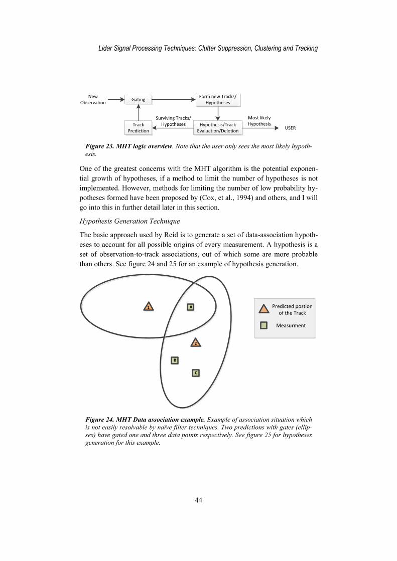
The algorithm proposed by Reid is a hypothesis oriented approach that main-tains the hypothesis structure from scan to scan and continually expands and cuts back, or prunes, the hypotheses as new data is received. Compatible tracks are defined to be tracks that do not share any common observations. Then, on the advent of new data, each hypothesis is expanded into a set of new hypothe-ses by considering all observation-to-track assignments for the track assignments for the tracks within the hypothesis (Blackman, et al., 1999). See figure 23 for a basic overview.


44

Figure 23. MHT logic overview. Note that the user only sees the most likely hypoth-esis.

One of the greatest concerns with the MHT algorithm is the potential exponen-tial growth of hypotheses, if a method to limit the number of hypotheses is not implemented. However, methods for limiting the number of low probability hy-potheses formed have been proposed by (Cox, et al., 1994) and others, and I will go into this in further detail later in this section.

Hypothesis Generation Technique

The basic approach used by Reid is to generate a set of data-association hypoth-eses to account for all possible origins of every measurement. A hypothesis is a set of observation-to-track associations, out of which some are more probable than others. See figure 24 and 25 for an example of hypothesis generation.

Figure 24. MHT Data association example. Example of association situation which is not easily resolvable by naïve filter techniques. Two predictions with gates (ellip-ses) have gated one and three data points respectively. See figure 25 for hypotheses generation for this example.

Gating

Track Prediction

Form new Tracks/Hypotheses

Hypothesis/Track Evaluation/Deletion

Surviving Tracks/Hypotheses

New Observation

USER

Most likely Hypothesis

1

2

A

B

C

Predicted postion of the Track

Measurment

Chapter 6 Tracking

45

Figure 25. MHT Hypothesis tree. This structure represents the hypotheses tree cre-ated for the example presented in figure 24. The first level (A) is created by meas-urement A, level B is created by measurement B, etc. There are four branches from the root node to level A. That is, measurement A either originates from noise (N), track 1, track 2 or an entirely new track 3. In the branch labeled “One hypothesis”, assuming that measurement A originated from track 1, measurement B can either originate from noise (N), track 2 or a entirely new track 4. The branch furthest to the left is the hypothesis that all measure originated from noise, while the branch furthest to the right is the hypothesis that all measurements originates from entirely new tracks. For this example, a total of 28 hypotheses where created.

Probability of each Hypothesis

The derivation for determining the probability of each hypothesis is a non-trivial task. I will here present the basic outlines of the probability calculations and re-sult, but leave it to the reader to explore the full derivation in (Reid, 1979), (Blackman, et al., 1999), (Bar-Shalom, et al., 1987) or (Cox, et al., 1994).

Let z(?) denote the observation collected and let Ω(?) = {Ω!(?), 9 = 1,2,3 … } the set of all hypotheses in time step k. The probability of hypothesis 9 given the collected observation is a Bayesian estimate,

\!(?) = \(Ω!(?)|z(?)). (27)

We may view Ω!(?) as the joint hypothesis formed from the prior hypothesis Ω!(? − 1) and the assosiation hypothesis for the current data set. After the deri-vation in equation 9 – 16 of (Reid, 1979), with the use of Bayes’ theorem, some extension and simplifying, we can rewrite (27) as

3

2 4

55 2N

N

52N N

1

2 4

55 2N

N

52N N

2

4

N 5

N

N 5

N

2 4

NN 2 5

N

N 2 5 5

Origin of measurment

C B A

One hypothesis


46

\!(?) = 1* \�� (1 − \�)��H�� ∙ ∙ �� (�" − 5̅, �)��

"'( � \�(? − 1) (28)

where 1/c is a combination of constants encountered during the derivation, \�� is the probability of detection for the �� previously known targets, \� is the probability of detection for new targets. �� is the number of (new) targets and �� is the number of previously known targets. �� is the density of false tar-gets and �� is the density of previously unknown targets. ( ) is the normal distribution pdf, described below, and �" is an observation from the sensor. H is the observation model and 5̅ is the state. � is the innovation covariance and \�(? − 1) is the prior hypothesis.

This equation looks daunting, but when split into its components it becomes more clear. \��(1 − \�)��H�� does in large perform the same role as the clut-ter suppression filter developed in section 0, and hence will not be further dis-cussed here. ∏ (�" − 5̅, �)��"'( is the product of outputs from the normal distribution with covariance S and the residual error as the expected value. Note that these parameters are estimated by the Kalman filter, in section 6.1.2 these parameters are available for review. The normal distribution pdf is given by

(5, �) = DH�7.�v��hjv��|�| .

(29)

Pruning and merging

Pruning is the process of excluding low-probability hypotheses, while attempt-ing to merge similar hypotheses. One way of pruning hypotheses is to select the n best hypotheses for continued processing, while another is to exclude all hy-potheses with a probability under a certain threshold.

Chapter 6 Tracking

47

Hypothesis merging can be accomplished by keeping track of the track initiation number, i.e. when you initiate a track, it is given a unique “root” number, which will remain with the track throughout its life span. Weak hypotheses will be pruned away, see figure 26. This technique can be incorporated into the hypoth-eses generation technique above by minimizing the number of improbable tracks, the number of improbable hypotheses can be minimized.

Figure 26. Combinatorial tree model for track merging. By keeping track of the track “root” number (r), the track number (t), and the observation number (o), a lot can be said about the tracks origin. Since track t3 and t4 share root track, they are likely to have very similar characteristics. Hence they can be merged and the least probable of the two be pruned away.

Two different tracking algorithms where implemented, the Local Nearest Neighbor (LNN) association filter and the Multi Hypothesis Tracking (MHT) filter.

The local NN using the fixed radius gating technique, with an estimator based only on the previous state, i.e. it is equivalent to the prediction stage of the Kal-man filter. This is a very naïve tracking algorithm, which performs well in envi-ronments without much clutter, close targets or unpredictable target dynamics. A class diagram of this algorithm which illustrates the algorithms classes, methods and variables is available in figure 27.

o0 o1 o2

r0 r1

t1

b1

t0

b0

t4

b4

t3

b3

t2

b2

Track initiation

Current track

Obser-vation


48

Figure 27. LNN algorithm class diagram. It is clear that this is a very simple algo-rithm with only two classes, four variables and one method.

The MHT filter demanded considerable more work to get into stable operation. It uses the linear Kalman filter as an estimator together with probabilistic gating to form the observations. A class diagram of the implemented MHT algorithm is available in figure 28.

Figure 28. MHT algorithm class diagram. The ”TrackHandeler” class is the main class, which creates ”Track” instances, which in turn has inherited the ”Kalman” class properties. The “Probability” class is used by the track handler to calculate the probability of each hypothesis.

+state : int+label : int+root : int

Track

+addObservation()+tracks : list

LNNInstance

+predict()+gate()+update()+updateStatus()

+status : int+label : int+missed : int+likelihood : float+prior : float+root : int+parent : int+label : int

Track

+getState()+predict()+residual()+update()

+state : Array+previousState : Array+T : float+Phi : Array+H : Array+P : Array+Q : Array+R : Array+y : Array+S : Array+K : Array

Kalman

+addObservation()+generateHypotheses()+generateTracks()+getUserTracks()+nextAvailableRoot()+numberOfTracks()+updateTrack()

+tracks : list+roots : list

TrackHandeler

+getCombos()+mostLikelyCombo()+probability()

+tracks : list

Probability

Inheritance Instance

Instance

Chapter 6 Tracking

49

This section will present the result of a series of trial runs conducted the two im-plemented tracking algorithms with simulated data. I will also present the big danger of running a MHT tracking algorithm without track pruning.

Several studies on the relative performance of LNN, GNN, PDA, JPDA and MHT tracking algorithms. See for example chapter 6.8 in (Blackman, et al., 1999), page 10-21 of (Chang, 2002) and (de Feo, et al., 1997).

In the following section I have attempted a similar comparison, but with a slight-ly different test setup.

The tracking algorithms where tested using Monte Carlo Simulations. A Monte Carlo simulation is conducted by averaging over a repeated number of simula-tions, in this case 100. A common way of conducting the Monte Carlo test, in-cluding the sources mentioned above, is to test two diagonal crossing tracks, like in figure 32.

However, for this simulation a slightly harder test was constructed. The test is made up of three constant velocity targets, initialized as described in table 3, moving in a 100 m x 100 m square. There are, besides the commonly used 90° encounter situation, also a 180° encounter. After initialization, we have the first close encounter, this one of 180°. The se-cond encounter 90° occurs shortly after this, here the two targets actually over-lap. See figure 29.


50

All targets have an additive Gaussian noise component, i.e., the measured posi-tion of the targets are 5[(?) = 5(?) + E and L[(?) = L(?) + E respectively, where w is zero mean Gaussian noise with variance = 1 m.

Table 3. Monte-Carlo simulation target parameters.

Target Number of data-points �� [�] �� [�] �̇� [�/�] �̇� [�/�]

A 20 0 60 5 0

B 20 60 0 0 5

C 20 65 60 0 -3

Chapter 6 Tracking

51

Figure 29. Monte-Carlo simulation targets. Three targets (A, B and C) are initial-ized in a). In b) we have the first close encounter, this one of 180°. The second en-counter (90°) occurs in c), here the two targets actually overlap. In d) all crossings have occurred. The arrow shows the target movement direction.

Two tracking algorithms where submitted to this simulation, the LNN and the MHT. The LNN algorithm used a circular type gating (see section 6.2.1) with �"uv = 10�. For this experiment, the MHT filter used KF parameters as de-scribed below. Note that these parameters could have been set to actually corre-spond to the values used by the simulation targets, but here a more general pa-rameter setup is presented. The MHT used probabilistic gating with x = 1. For a more comprehensive introduction to the KF parameters, see section 6.1.2.


52

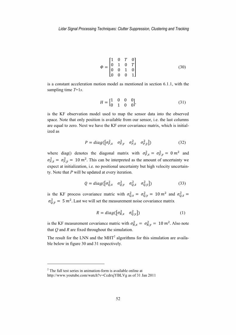
^ = P1 0 Q 00 1 0 Q0 0 1 00 0 0 1R (30)

is a constant acceleration motion model as mentioned in section 6.1.1, with the sampling time T=1s.

= p1 0 0 00 1 0 0s, (31)

is the KF observation model used to map the sensor data into the observed space. Note that only position is available from our sensor, i.e. the last columns are equal to zero. Next we have the KF error covariance matrix, which is initial-ized as

\ = �9��(�ye,v ye,� ye,v̇ ye,�̇ �) (32)

where diag() denotes the diagonal matrix with ye,v = ye,� = 0 � and ye,v̇ = ye,�̇ = 10 �. This can be interpreted as the amount of uncertainty we expect at initialization, i.e. no positional uncertainty but high velocity uncertain-ty. Note that P will be updated at every iteration.

O = �9��(�y ,v y ,� y ,v̇ y ,�̇ �) (33)

is the KF process covariance matric with y ,v = y ,� = 10 � and y ,v̇ = y ,�̇ = 5 �. Last we will set the measurement noise covariance matrix

� = �9��(�yd,v y ,� �) (1)

is the KF measurement covariance matric with yd,v = yd,� = 10 �. Also note that Q and R are fixed throughout the simulation.

The result for the LNN and the MHT2 algorithms for this simulation are availa-ble below in figure 30 and 31 respectively.

2 The full test series in animation-form is available online at http://www.youtube.com/watch?v=CcdrxjYBLVg as of 31 Jan 2011

Chapter 6 Tracking

53

Note the difference scale of the square residual error. This is due to the LNN:s incapability to handle multiple targets. It becomes obvious that the MHT outper-forms the LNN with great results.

Figure 30. LNN Simulation result. Estimated trajectories to the left, with estimated square residual error to the right. Note that only track A was tracked successfully.

Figure 31. MHT Simulation result. Estimated trajectories to the left, with estimated square residual error to the right. Note that no track was lost during this test, but the square errors increase right at initialization and whiles a close encounter.


54

As mentioned in section 6.2.5, the MHT track pruning function is absolutely critical for an effective operation. Figure 32 shows how large effect x had on an MHT system with probabilistic gating without track/hypothesis pruning.

Figure 32. The MHT algorithm without track pruning. With increased x, the probabilistic gating covered in section 6.2.1 allows for an exponential growth of the number of tracks.

Chapter 7 Discussion

55

This chapter will attempt to discuss the results obtained in this thesis and point out what went well and what was not implemented due to a lack of time. This will extend into a discussion on what could be accomplished if the work pre-sented in this thesis where to be continued.

In this thesis solutions to three different problems encountered when working on scanning sensor systems, specialized to be used in laser scanning systems, was presented.

The clutter suppression filter developed was based on knowledge of the noise distribution and density estimation of tentative targets. The filter showed good results with a limited computational load.

The clustering algorithm developed appears to work very well for the high SNR condition available at most conditions encountered by the Lidar system. The clustering toolbox provided a good insight to the type of data suitable for use with this filter, and allowed for parameter tuning to be fast and accurate.

The performance of the MHT algorithm was shown to be very good, especially for the crossing tracks problem, which is one of the greatest challenges for any tracking system. However, the timescale for implementing a robust tracking al-gorithm was vastly under estimated. While the time needed to implement a naïve algorithm such as the LNN can be done in one day, the MHT algorithm took several months.

One remark on this subject that should be mentioned is that the tracking algo-rithms where implemented but not integrated. This was due to a lack of time, since the existing system which the tracking was to be implemented on was con-structed for slightly different purposes.


56

This Master Thesis was conducted during a limited time, which means that many things more could have been investigated. Improvement could be made to both the hardware and software presented in this thesis.

An example of hardware that could be further investigated is the laser ranger. Laser ranger units operating at longer wavelengths (~1500nm) should be inves-tigated, since the longer wavelengths are less easily disturbed by atmospheric noise. Another advantage with these devices is that they allow for a higher out-put power while maintaining an eye safe classification.

The main disadvantages of ~1500nm lasers is the higher costs and the lower base of knowledge on this technology compared to visible and near visible laser systems.

The dynamic properties of the atmospheric noise should be further investigated. There is a lack of scientific material on this subject, in the context of light based ranging, which could lead to the development of new and effective filters.

The precipitation filter developed in this thesis should be investigated further during a more varied range of precipitation (rain, hail, sleet etc.). Since this filter was developed during the Swedish winter, only snow was available for testing.

It should be mentioned that access to scanner data collected during dense fog was available, but due to time constraints, this data was not further analyzed.

Another interesting approach to this problem would be to implement a multiple dynamic model approach, like the one suggested in section 6.1.1 for estimation. This multiple model approach would incorporate a filter bank with one filter trimmed for each atmospheric condition, merging filters that are similar in char-acter. This would allow not only having an optimal filter for each atmospheric condition, but this filter bank could also be used as a “weather classifier”.

The clustering algorithm developed in this thesis was shown to work for many types of data. However, since laser based ranging have a high SNR level under most (good) conditions, this algorithm was optimized for high SNR scenarios. For a sensor system more exposed to intrinsic or extrinsic noise, a distribution based clustering method, such as the Expectation Maximization algorithm should be investigated.

Chapter 7 Discussion

57

As discussed in chapter 7.1, the tracking algorithm was implemented but not integrated into the existing Lidar system. This should be completed in order to fully benefit from the Lidars advantages.

The topic of estimation and data association was the part which most time and effort was being spent. As of the Kalman estimator, a lot of effort can be spent trimming the covariance parameters, to achieve an optimal estimator.

As for data association, MHT has good performance, but is very complex. It would be interesting to further investigate relatively simple techniques that have low complexity but adequate performance.

There is no shortage on literature on tracking; for example, the reference section of chapter 6 (Data Association) in (Blackman, et al., 1999) holds 110 papers, books and studies on the subject!


58

Chapter 8 References

59

Amann, Markus-Christian, et al. 2001. Laser ranging: a critical review of usual techniques for distance measurement. Optical Engineering. 2001, Vol. 40.

Bar-Shalom, Yaakov and Fortmann, T. E. 1987. Tracking and Data Association. San Diego, CA, USA : Academic Press, 1987.

Bar-Shalom, Yaakov and Tse, E. 1975. Tracking in a Cluttered Environment with Probabilistic Data Association. Automatica. Sept, 1975, Vol. II.

Bar-Shalom, Yaakov, Daum, Fred and Huang, Jim. 2009. The Probabailistic Data Association Filter. IEEE Control Systems Magazine. December, 2009.

Bidigare, Pat. 2004. Minimum radar cross section bounds for passive radar responsive tags. Signals, Systems and Computers, 2004. Conference Record of the Thirty-Eighth Asilomar Conference on. 2004, Vol. II.

Blackman, Samuel and Popoli, Robert. 1999. Design and Analysis of Modern Tracking Systems. Boston, MA. : Artech House, 1999.

Chang, Kou-Chu. 2002. SYST680: Principles of C3I #4. Fairfax, Virginia : Department of Systems Engineering, George Mason University, 2002.

Cox, Ingemar J. and Hingorani, Sunita L. 1994. An Efficient Implementation and Evaluation of Reid's Multiple Hypothesis Tracking Algorithm for Visual Tracking. Princeton, NJ : NEC Research Institute, 1994.

Cracknell, Arthur P. and Hayes, Ladson. 2007. Introduction to Remote Sensing. New York, NY : The Guilford Press, 2007.

de Feo, M., et al. 1997. IMMJPDA versus MHT and Kalman filter with NN correlation: performance comparison. Radar, Sonar and Navigation, IEE Proceedings. 1997, Vol. 144, No. 2.

Embsec. vFence S-500 Product Description. [Online] http://embsec.com/index.php/en/products/vfence-s-500 (January 2011).

Haines, Eric. 1994. Graphical Gems IV. Boston, MA : Academic Press, 1994.


60

Hong, Lang. 1999. Multirate interacting multiple model filtering for target tracking using multirate models. IEEE Transactions on Automatic Control. 1999, Vol. 44, 7.

Kalman, Rudolf E. 1960. A New Approach to Linear Filtering and Prediction Problems1. Transactions of the ASME–Journal of Basic Engineering,. 82, 1960.

Kurien, T. 1990. Issues in the Design of Practical Multitarget Tracking Algorithms. Multitarget-Multisesnor Tracking: Advanced Applications, Artech House, MA. 1990.

MDL Laser Systems. MDL LaserAce ILM Product Description. [Online] http://www.mdl.co.uk/laser_modules/laserace-ilm/index.html (January 2011).

Reid, Donald B. 1979. An Algorithm for Tracking Multiple Targets. IEEE Transactions on Automatic Control. December, 1979, Vols. AC-24, 6.

Rice, John. 1995. Mathematical Statistics and Data Analysis (Second ed.). s.l. : Duxbury Press, 1995. ISBN 0-534-20934-3.

Schleher, D. C. 1976. Radar Detection in Weibull Clutter. IEEE Transactions on Aerospace and Electronic Systems. 1976, Vols. AES-12, November.

Sorenson, H. W. 1970. “Least-Squares estimation: from Gauss to Kalman”. IEEE Spectrum,. 1970, Vol. 7.

Tan, Pang-Ning, Michael, Steinbach and Vipin, Kumar. 2005. Introduction to Data Mining. Boston, MA : Addison Wesley, 2005.

Welch, Greg and Bishop, Gary. 2006. An Introduction to the Kalman Filter. Chapel Hill, NC : Department of Computer Science, University of North Carolina, 2006.

Wiener, Norbert. 1949. The Extrapolation, Interpolation and Smoothing of Stationary Time Series. New York, NY : John Wiley & Sons, 1949.

1

vFence S-500 is a Lidar intended for object detection and classification. With a high accuracy range of up to 500 meters it observes people, vehicles or other objects and analyzes its position, size and velocity. The laser distance meter works without reflectors and detects both static and moving objects (Embsec).

Figure 33. The Embsec vFence S-500. Photo courtesy of Embsec AB, Sweden.

Specifications:

Range (m) Up to 500

Field of View (degrees) 270

Distance Accuracy (cm) 10

Angular Resolution (degrees) 0.05

Power Consumption 30W @ 24V

Interface Ethernet

Weight 15 kg

Intended Use Outdoor


2

The ILM (Industrial Laser Module) OEM Laser Modules are compact class 1 eye safe, rugged, multipurpose laser distance meters for integration into OEM applications (MDL Laser Systems).

Figure 34. The MDL ILM T 500. Photo courtesy of MDL Laser Systems, UK.

Specifications:

Model ILM T 150 ILM T 500

Wavelength (nm) 905 905

Beam Divergence (mrad) 2.5 x 0.2 2.0 x 0.2

Reflector less Range (m) 0.5 – 150 2 – 500

Max range (m) 630 2000

Accuracy (cm) 30 30

Resolution (cm) 10 10

Rep Rate (Hz) 400 1000

Eye Safety Class 1 Class 1

lidar signal processing techniques 9 may - diva portal470911/fulltext01.pdf · 1 introduction ......

Documents