lidar-derived high quality ground control information and ... · lidar-derived high quality ground...
TRANSCRIPT

1
LiDAR-Derived High Quality Ground Control
Information and DEM for Image Orthorectification
XIAOYE LIU, ZHENYU ZHANG, JIM PETERSON AND SHOBHIT CHANDRA
Center for GIS, School of Geography and Environmental Science, Monash University,
Wellington Road, Clayton, VIC 3800, Melbourne, Australia
E-mail: {Xiaoye.Liu, Zhenyu.Zhang, Jim.Peterson, Shobhit.Chandra}@arts.monash.edu.au
Abstract
Orthophotos (or orthoimages if in digital form) have long been recognised as a
supplement or alternative to standard maps. The increasing applications of
orthoimages require efforts to ensure the accuracy of produced orthoimages. As
digital photogrammetry technology has reached a stage of relative maturity and
stability, the availability of high quality ground control points (GCPs) and digital
elevation models (DEMs) becomes the central issue for successfully implementing an
image orthorectification project. Concerns with the impacts of the quality of GCPs
and DEMs on the quality of orthoimages inspire researchers to look for more reliable
approaches to acquire high quality GCPs and DEMs for orthorectification. Light
Detection and Ranging (LiDAR), an emerging technology, offers capability of
capturing high density three dimensional points and generating high accuracy DEMs
in a fast and cost-effective way. Nowadays, highly developed computer technologies
enable rapid processing of huge volumes of LiDAR data. This leads to a great
potential to use LiDAR data to get high quality GCPs and DEMs to improve the
accuracy of orthoimages. This paper presents methods for utilizing LiDAR intensity
images to collect high accuracy ground coordinates of GCPs and for utilizing LiDAR
data to generate a high quality DEM for digital photogrammetry and orthorectification
processes. A comparative analysis is also presented to assess the performance of
proposed methods. The results demonstrated the feasibility of using LiDAR intensity
image-based GCPs and the LiDAR-derived DEM to produce high quality orthoimages.
Keywords: orthorectification, orthoimage, LiDAR, LiDAR intensity, DEM

2
1. Introduction
Advances in computer hardware and software as well as newly emerging technologies,
such as sophisticated remote sensing technology and Light Detection and Ranging
(LiDAR) systems, have promoted the significant development of traditional spatial
mapping procedures. One of the examples is the application of high quality digital
orthophotography as a major data source to maintain and update standard maps.
Orthophotos, also known as orthoimages if in digital form, are computer-generated
images of aerial photographs in which displacements caused by camera or sensor tilts
and terrain relief have been removed. As digital orthoimages contains more semantic
and visible information than traditional maps, they have great potential of extracting
more accurate spatial information for fast updating maps or Geographical Information
System (GIS) database.
Quality is essential when using orthoimages in various applications. Errors that affect
the quality of orthoimages come from each step of the orthorectification processing.
Li et al analysed the main factors that affect digital orthoimage accuracy, including
aerial photograph scanning, interior orientation, exterior orientation, and differential
rectification [32]. As digital photogrammetry technology has reached a stage of
relative maturity and stability, the availability of high quality ground control points
(GCPs) and digital elevation models (DEMs) becomes the central issue for
successfully implementing an image orthorectification project [4], [49]. Concerns
with the impacts of the quality of GCPs and DEMs on the quality of orthoimages
inspire researchers to look for more reliable approaches to acquire high quality GCPs
and DEMs for orthorectification.

3
Traditionally, the ground control points are obtained either from field survey
(including GPS (Global Positioning System) surveying) or by interpretation of
existing orthoimages or topographic maps. Although the former method may achieve
a higher accuracy for GCPs, it is really time consuming and labour intensive; the
drawback of the latter one is the accuracy limitation. Similarly, generating DEMs by
field survey or by interpretation of existing topographical maps is neither cost-
effective nor reliable. Therefore, specialists in photogrammetry are continuing to look
for appropriate approaches to obtaining high quality GCPs and DEMs for image
orthorectification processing.
LiDAR, an emerging technology, offers capability of capturing high density and high
accuracy three dimensional points in a fast and cost-effective way. One of the
appealing features in the LiDAR output is the direct availability of three dimensional
coordinates of points in the object space [25]. In addition, most LiDAR systems also
have the capability to capture the intensity of the backscattered laser pulse. Although
the backscattered LiDAR intensity values are a function of many variables, to some
extent, LiDAR intensity data represent the material characteristics of the targets hit by
the laser beam. Moreover, LiDAR intensity images have orthogonal geometry
characteristics and have high spatial resolution. Ground objects, especially those
commonly used for ground controls, such as the intersection of roads and intersection
of agricultural plots of land, can be identified from the LiDAR intensity image that
corresponds to an aerial image. Therefore, the LiDAR intensity images offer a good
alternative of GCPs collection for aerial triangulation calculation in digital
photogrammetry. In addition, LiDAR data facilitate the derivation of high accuracy
and high resolution DEMs. Our previous research work demonstrated that LiDAR

4
offers advantages over traditional methods for representing a terrain surface [33], [34].
The advantages refer to accuracy, resolution, and cost. Nowadays, highly developed
computer technologies enable rapid processing of huge volumes of LiDAR data,
which leads to a great potential to use LiDAR data to get high quality GCPs and
DEMs to improve the accuracy of orthoimages.
Rapid maturation of LiDAR technology, continuous falling of prices and increasing
accuracy of LiDAR data are causing an exponential availability of LiDAR datasets
[25]. However, it is impossible for LiDAR data to replace the traditional remotely
sensed imagery because LiDAR data cannot provide as much semantic information as
remotely sensed images can. A growing body of research has demonstrated the
complementary nature of LiDAR data and traditional remotely sensed data such as
aerial photography and mutilspectral or hyperspectral imagery in terms of their
geometrical and semantic information [12], [25], [26]. Habib et al presented an
approach for using linear features derived from LiDAR data into photogrammetric
model to align the photogrammetric model relative to the LiDAR reference frame [26].
Their research provided a good alternative for photogrammetric modelling, except for
point-based models. Nevertheless, little research has been done for directly using
LiDAR’s high quality geometric data (particularly, the valuable LiDAR intensity
images) for GCPs which are required for aerial triangulation calculation, and for using
LiDAR-derived high quality DEMs for orthorectification processing, especially with
the utilization of commonly-used point-based commercial digital photogrammetric
systems and with no need to develop additional algorithm .
5
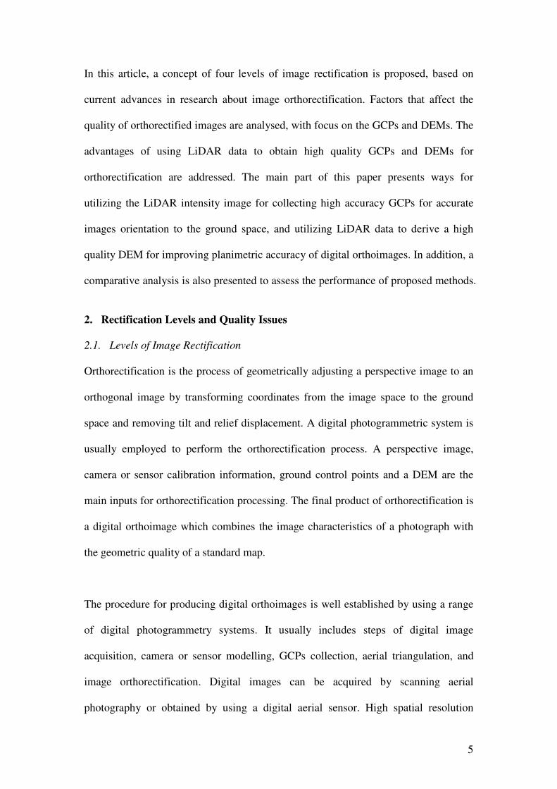
In this article, a concept of four levels of image rectification is proposed, based on
current advances in research about image orthorectification. Factors that affect the
quality of orthorectified images are analysed, with focus on the GCPs and DEMs. The
advantages of using LiDAR data to obtain high quality GCPs and DEMs for
orthorectification are addressed. The main part of this paper presents ways for
utilizing the LiDAR intensity image for collecting high accuracy GCPs for accurate
images orientation to the ground space, and utilizing LiDAR data to derive a high
quality DEM for improving planimetric accuracy of digital orthoimages. In addition, a
comparative analysis is also presented to assess the performance of proposed methods.
2. Rectification Levels and Quality Issues
2.1. Levels of Image Rectification
Orthorectification is the process of geometrically adjusting a perspective image to an
orthogonal image by transforming coordinates from the image space to the ground
space and removing tilt and relief displacement. A digital photogrammetric system is
usually employed to perform the orthorectification process. A perspective image,
camera or sensor calibration information, ground control points and a DEM are the
main inputs for orthorectification processing. The final product of orthorectification is
a digital orthoimage which combines the image characteristics of a photograph with
the geometric quality of a standard map.
The procedure for producing digital orthoimages is well established by using a range
of digital photogrammetry systems. It usually includes steps of digital image
acquisition, camera or sensor modelling, GCPs collection, aerial triangulation, and
image orthorectification. Digital images can be acquired by scanning aerial
photography or obtained by using a digital aerial sensor. High spatial resolution

6
satellite imagery is also an increasingly popular data source for producing
orthoimages. Camera/sensor modelling is referred to as interior orientation which
defines a camera/sensor’s interior geometry as it existed at the time of image capture.
Camera calibration information and the measurement of fiducial marks are the
primary input for the interior orientation which transforms the image from pixel
coordinate system to the image space coordinate system.
In order to define the position and direction orientation of the camera that captured an
image, GCPs are required to establish a mathematical relationship between images,
camera/sensor, and the ground by using the following collinearity condition equations:
)()()(
)()()(
033032031
0130120110
ZZmYYmXXm
ZZmYYmXXmfxx
−+−+−
−+−+−⋅−=
)()()(
)()()(
033032031
0230220210
ZZmYYmXXm
ZZmYYmXXmfyy
−+−+−
−+−+−⋅−=
where ,0X 0Y and 0Z define the position of the camera station with respect to the
ground space coordinate system (X, Y and Z); 0x and 0y are the position of the
principal point in the image coordinate system (x, y); f is the focal length of the
camera; and ,11m ,12m …, and 33m are the elements of the rotation matrix. The
rotation matrix is derived by applying a sequential rotation of ω about the x-axis, φ
about the y-axis, and κ about the z-axis [24]. Once collinearity equations are
formulated by using enough ground control and tie points, the least squares
adjustment method is used to implement the block triangulation calculation, the
results from which are then used as the primary input for the image orthorectification
process.

7
Depending on the input data for the process and the degree of removal of
displacement, image rectification usually can be classified as three levels [30],
orthorectification being the highest level of the rectification. If nominating raw digital
images as the products of level 1, the level 2 rectification processes raw central
perspective images with the inputs of orientation parameters and GCPs, but without
the information of relief. The resulting product of level 2 processes can be called a
‘vertical-image’, with tilt displacements being eliminated in the rectified image. The
level 3 process adds a further rectification for terrain relief by use of a DEM. On
completion of level 3 rectification, the effects of central perspective and
displacements due to tilt and terrain relief have been removed so that the resulting
image is an orthographic product with a consistent scale. The level 3 rectification is
usually referred to as the orthorectification. Recently, the awareness of the concept of
‘true orthoimage’ in which the displacements due to terrain and buildings or trees are
removed is increasingly acknowledged. In the collinearity equations, for a given set of
(X, Y, Z), a set of (x, y) should be uniquely resolved, which means that any pixel in
the orthoimage has one and only one corresponding pixel in the perspective image.
However, in urban or forested area, tall buildings and trees appear oblique and may
occlude other objects in the images. As a result, more than one set of (X, Y, Z) points
may be projected to the same point (x, y) in the image space. The geometric
implication of this many-to-one relationship is referred to as occlusion [45]. In the
process of true-orthorectification, a digital surface model (DSM) or a canopy surface
model (CSM) or a digital building model (DBM) is employed [8], [45], [56], [57], and
the algorithm of removal of occlusion is the core of this process. Here, we nominate
this kind of true orthoimage as the product of level 4. The workflow of four levels of
rectification with required input data is illustrated in Figure 1.

8
Scanned
Aerial Photography
Scanned
Aerial PhotographyCamera/Sensor
Calibration Information
Camera/Sensor Calibration Information
Interior OrientationInterior Orientation
Rectification withoutRelief Information
Rectification without
Relief Information DEMDEM
Aerial TriangulationAerial Triangulation
DSMDSMDifferentialRectification
Differential
RectificationDifferential
Rectification
Differential
Rectification
OrthoimageOrthoimage
Occlusion
Removal
Occlusion Removal
Level 1
Level 2
Level 3
Level 4
GCPs GCPs
True
Orthoimage
True
Orthoimage
Rectified ImageRectified Image
Figure 1. Orthorectification workflow for different levels of products.
The utility of the raw image in practice is limited due to its orthogonal geometric
nature and displacements. Objects extracted from level 2 images are more reliable
than those from raw images because of their perspective geometric characteristics. In
flatter area they have limited relief displacement effects. The most commonly used
orthoimages are those from level 3. These perspective images are theoretically free of
displacements caused by terrain relief, and have consistent scales. Therefore, features
from these images are represented at their correct locations. Distances and angles can
be directly measured on level 3 images. For the product of level 4, it has a particular
use with large scale of orthoimage in urban or forested areas where displacements
caused by buildings or trees could be significant. As the study area of this project is in
rural area, the emphasis at this stage is on the process for generating level 3
orthoimags.

9
2.2. Quality Issues of Image Rectification
Throughout the orthorectification process, a wide range of factors can affect the
quality of an orthorectified image [31]. The main scope for error generation exists in
the processes of image scanning, interior orientation, exterior orientation, and
differential rectification. Image scanning is the process of converting an analogue
aerial image to a digital image by using a photogrammetric-quality scanner. The
analogue aerial image can be in paper print or film transparency format. Image data
can be captured either in reflection modes from paper prints or in transmission mode
from film transparencies. Compared to paper prints, film transparencies are the
preferred source materials when converting aerial photographs to digital images. Not
only are they more dimensionally stable, but also they tend to have higher spatial
resolutions and a greater range of grey values [54]. However, paper prints are still the
major source materials used for converting to digital images. The accuracy of a
converted digital image is mainly dependent on the accuracy of the scanner and the
available resolution. For photogrammetric applications, a scanner should be able to
scan aerial images (23 x 23 cm) with a minimum optical resolution of 600 dpi, thus
providing sufficient radiometric resolution (8 bits with value from 0 - 255 for black
and white image or 24 bits - 8 bits for each channel of a colour image) and high
geometric accuracy (4 - 12.5 µm minimum pixel size) [10], [11]. The pixel size of
scanned aerial images is a function of image scale and scanning resolution selected,
and can be calculated by the formula:
pixel_size = resolutionscanning
scaleimage
_
_
For example, if scanning an aerial image with a scale of 1:25,.000 by using a scanning
resolution of 800 dpi (dots per inch), each pixel in the scanned image will represent

10
31.25 by 31.25 inches (0.794 by 0.794 m) on the ground. Since every subsequent
photogrammetric processing step is based on the scanned imagery, it is important to
use a high resolution scanner and select a suitable scanning resolution so that the
original image quality can be preserved [32].
The quality of the interior orientation parameters is contingent on the measurement of
the photo fiducial marks and the camera calibration information. Therefore, accurate
fiducial mark measurement and access to an accurate camera calibration report are
crucial if a high quality calculation of interior orientation parameters is to be attained.
As far as the quality of exterior orientation parameters and differential rectification is
concerned, the quality of GCPs and DEMs is extremely important for the calculation
of these two processes. The GCPs and DEMs are the focus of this paper in terms of
the analysis of orthoimage quality.
The role of GCPs is to establish an accurate mathematical relationship between the
images, the camera/sensor, and the ground so that the exterior orientation parameters
of each aerial photograph can be determined. Any inaccuracy of ground control
information affects the accuracy of exterior orientation parameters calculated by aerial
triangulation, and finally are propagated into the orthorectified images. The absolute
accuracy of orthoimages is largely dependent on the quality and the distribution of the
GCPs used to orient the image to the ground space [45].
For generation of digital orthoimages from perspective images, a DEM must be used
in performing the differential rectification. The role of the DEM is to eliminate the
effects of terrain relief displacement. DEM quality is very important to the

11
orthorectification process because both vertical and horizontal errors in the DEM will
be propagated to resulting digital orthoimages, appearing as planimetric (horizontal)
errors in the orthoimages. DEM quality becomes more significant to orthorectification
process as local relief increases.
3. LiDAR and Potential Advantages of Using LiDAR-Derived GCPs and DEMs
3.1. LiDAR Systems
LiDAR is an active remote sensing technology. It actively transmits pulses of light
toward an object of interest, and receives the light that is scattered and reflected by the
objects. The distance (range) between the LiDAR sensor and the object can be
calculated by multiplying the speed of light by the time it takes for the light to
transmit from and return to the sensor [50], [53]. The light used by LiDAR systems
varies with applications, depending on the targets to be detected (e.g., their light
scattering properties), and the range between the LiDAR sensor and the targets. It
could be in the ultraviolet, visible, and near infrared portions of the electromagnetic
spectrum [17]. For example, ultraviolet light can be used to detect water vapour in the
atmosphere, and near infrared light to detect topographic objects, or ozone, aerosol,
and pollutants in the atmosphere [2], [17], [37], [39].
For terrain mapping purpose, an airborne LiDAR system is typically composed of a
laser scanner unit, a differential Global Positioning System (dGPS) receiver, and an
Inertial Measurement Unit (IMU) [15], [27], [44], [51]. The GPS receiver is used to
record the aircraft trajectory at centimetre level and the IMU measures the attitude of
the aircraft (roll, pitch, and yaw or heading) [51]. The laser scanner unit consists of a
pulse generator of Nd:YAN laser with a wavelength in the range of 0.8 µm to 1.6 µm
(typically, with 1.064 µm) and a receiver to get the signal of scattered and reflected

12
pulses from targets [41], [52]. The laser pulses are typically 10 to 15 ns in duration
and have peak energy of several millijoules [2], [52]. Laser pulses are emitted at a rate
of 2 kHz to 25 kHz to the Earth surface [3]. The range or distance between the
scanner and the target (calculated as stated above) and the position and orientation
information obtained from the GPS and IMU to determine target location with high
accuracy in three dimensional spaces. The three dimensional points are captured as
latitude, longitude, and ellipsoidal height based on the WGS84 reference ellipsoid.
They can be transformed to a national or regional coordinate system. At the same time,
elevations are converted from ellipsoidal heights to ortho-metric heights based on a
national or regional height datum by using a local geoid model [51]. Currently,
LiDAR data are typically delivered as tiles in ASCII files containing x, y, z
coordinates, and (as clients demand) with LiDAR intensity values.
LiDAR systems are also capable of detecting multiple return signals for a single
transmitted pulse [19], [44], [52]. Most LiDAR systems typically record first and last
pulse, but some are able to record up to five returns for a single pulse [48]. Multiple
returns occur when a laser pulse strike a target that does not completely block the path
of the pulse and the remaining portion of the pulse continues on to a lower object.
This situation frequently occurs in forested areas where there are some gaps between
branches and foliage [44]. Recording multiple returns is quite useful in the description
of forest stand and structure. Furthermore, a canopy surface model (CSM) generated
by using first returns from the canopy top can be used to generate true orthoimages in
forested areas [45].

13
The raw LiDAR data are three dimensional point clouds. Laser returns are actually
recorded from no matter what target the laser beam happens to strike [15], including
everything on the ground such as buildings, telephone poles, and power lines. The
post-processing of LiDAR data involves the removal of undesirable points and the
separation of the bare-earth data from the whole dataset by using filter algorithms [55].
The desired target for DEM generation is the bare-earth. Once the bare-earth points
are determined, a high accuracy and high resolution DEM can be generated. The high
accuracy and high resolution DEM provides terrain data of high enough quality to
refine greatly the elimination of relief displacement during orthorectification.
In addition to the three dimensional coordinates, most LiDAR systems also have the
capability to capture the intensity of the backscattered laser pulse. The backscattered
laser signal is a function of many variables such as the transmitted laser power, laser
beamwidth, range, atmospheric transmission, and effective target cross section (the
effective area for collision of the laser beam and the target). The target cross section is
strongly dependent on the target reflectance at the laser wavelength, the target area,
and the target orientation with respect to the incoming laser beam [20], [28], [43], [48].
The optical signal received by the sensor is converted to an electrical signal by a
photodetector (typically an avalanche photodiode). The generated photocurrent or
voltage is then quantized to a digital number (usually expressed in percent value,
representing the ratio of strength of reflected light to that of emitted light [47]) which
is referred to as the LiDAR intensity value for the particular return [14], [20], [28].
The LiDAR intensity data then can be interpolated to a geo-referenced intensity image
with orthogonal geometry.

14
Recently, there have been a few attempts to use LiDAR intensities in glacier
monitoring, land cover classification, and forest type identification [9], [13], [36], [40],
[47]. However, it should be noted that the backscattered LiDAR intensity values are a
function of many other variables in additional to the material characteristics of the
targets hit by the laser beam. Furthermore, unlike aerial photography or multispectral
satellite imagery, LiDAR intensity data contain information about objects’ reflectance
at only a specific wavelength (e.g., 1.064 µm). All of these factors will adversely
influence the application of LiDAR intensity data (especially for the application of
intensity data for land cover classification) unless the LiDAR intensity data have been
radiometrically calibrated [20], [27], [29], [42], [43].
In this project, however, since the LiDAR data have high spatial resolution, many
ground objects, especially those commonly used for ground controls such as the
intersection of roads and intersection of agricultural plots of land can be easily
recognized from LiDAR intensity images. In addition, LiDAR intensity images have
orthogonal characteristics. Therefore, it should be possible to directly collect higher
accuracy ground coordinates of GCPs from intensity images for digital
photogrammetric process.
Airborne LiDAR is still a rapidly growing technology. An important development is
the integration of a high resolution digital camera or a digital video camera with a
LiDAR system [3], [5]. For each collected digital image, the position and orientation
of the camera can be obtained by using the GPS and IMU data. Exterior orientation
parameters for each frame of imagery are directly provided by these position and
orientation data. Therefore, no stereo overlapping images and/or ground control points
are needed. Orthorectification can be completely automatic by using the digital

15
images and a LiDAR-derived DEM [5]. It is expected that the LiDAR system can be
combined with multispectral or hyperspectral imaging systems, which will result in
highly versatile systems and extended LiDAR application potential [3].
3.2. Potential Advantages of Using LiDAR-Derived GCPs and DEMs
The availability of increasingly sophisticated and automated digital image processing
systems has facilitated the use of photogrammetric techniques in a wide range of
applications [13]. However, the quality of GCPs and DEMs has been a big concern in
the production of digital orthoimages. The availability of high accuracy GCPs and
DEMs becomes the key issue for successful implementation of an image
orthorectification project.
As stated in section 1, traditionally, GCPs can be collected from field survey (using
total station or GPS), topographic maps, and national or state spatial infrastructure
data. All these methods are either time consuming and labour intensive or lack of
enough accuracy. In practice, in order to increase the redundancy that is beneficial for
gross error detection, and to prepare independent GCPs check points, it is quite
common to use more GCPs than minium number of GCPs required for the block
triangulation. Moreover, to ensure the calculation quality, GCPs should be evenly
distributed over the image covered area. It is a very difficult task for collecting a large
number of high quality GCPs by using traditional methods to meet all the
aforementioned requirements for digital photogrammetric and orthorectification
process.
DEMs are commonly generated from such datasets as topographic maps, stereo aerial
photography, satellite imagery or field survey. The drawbacks of using these kinds of
16
ways for DEM generation are either their limitations of accuracy or their labour
intensity. Fortunately, LiDAR offers the capability of capturing high density points
and high accuracy digital elevation data in a fast and cost-effective way. It has great
potential to provide high quality of GCPs and DEMs for orthorectification process
requirements.
There are significant advantages of using LiDAR data to provide GCPs and DEMs for
orthorectification process. First, the increasing availability of LiDAR data makes it
possible to provide high accuracy three dimensional points with high density and even
distribution over large areas. Second, due to its high accuracy and high visual
interpretable nature of intensity image, high quality GCPs can be directly picked up
from this image. Third, with high resolution and high accuracy LiDAR-derived DEMs,
it is possible to remove relief displacement at complicated terrain conditions. Finally,
LiDAR enables rapid acquisition of three dimensional points and intensity over large
areas so that the labour expenditure and other costs can be reduced since time is
money. However, it should be noted that the LiDAR market is not stable because the
LiDAR technology is in a development stage [12]. The cost of LiDAR data
acquisition can vary, depending on size of project, point density, and project location.
It is evident that, using LiDAR to collect data and generate DEM is a cost effective
way, comparing with field survey (using total station or GPS), especially over a large
area. Therefore, it is no doubt an economical way for GCPs collection by using
LiDAR intensity data which is a by-product of a LiDAR terrain mapping project.
4. Study Area, Data and Method
4.1. Study Area

17
The study area is in the region of Corangamite Catchment Management Authority
(CCMA), which is located in the south western Victoria, Australia. The landscape in
the region can be depicted to north and south highlands and a large Victoria Volcanic
Plain (VVP) in the middle. LiDAR data for the total area of 6900 km², covering most
part of VVP in the CCMA, were collected over the period of 19 July 2003 to 10
August 2003. These areas have high priority for a range of research projects
pertaining to environment management issues addressed in the catchment
management strategy plan. The primary purpose of these LiDAR data is to accurately
represent terrain pattern in this area, and combining with aerial photography, satellite
imagery, and other spatial data, to implement a serious of environment related
projects.
4.2. Data
The estimate of accuracy of LiDAR data used for this project is documented as 0.5
metres for vertical accuracy and 1.5 metres for horizontal accuracy [1]. LiDAR data
were first classified into bare-earth and non-ground points using different algorithms
across the project area [1]. Manual checking and editing of the data were also
conducted to further improve the quality of the classification [1]. The bare-earth
LiDAR points were used to generate a grid DEM.
Interpolation methods available for constructing a DEM from sample elevation points
can be classified: deterministic methods such as inverse distance weighted (IDW)
(assumes that each input point has a local influence that diminishes with distance) and
spline-based methods that fit a minimum-curvature surface through the sample points;
and geostatistical methods such as Kriging that takes into account both the distance
and the degree of autocorrelation (the statistical relationship among the sample points).
18
New or modified interpolation methods are still being developed [7], [46]. To
evaluate the performance of some commonly-used interpolation methods, several
comparisons of these interpolators have been conducted for different practical
purposes [6], [16], [18], [35], [38], [58]. None of the interpolation methods is
universal for all kinds of data sources, terrain patterns, or purposes. However, if
sampling data density is high, the IDW method performs well, even for complex
terrain [6], [16], [18]. LiDAR data have high sampling density, and so the IDW
approach was selected as the interpolator for our LiDAR data processing. Using
ArcGIS software, a regular 5 by 5 meters grid DEM and a DSM were created by using
the elevation values of the bare-earth points and all the points separately. Meanwhile,
LiDAR intensity data were also interpolated into a raster image with the spatial
resolution of one metre by using all the LiDAR points.
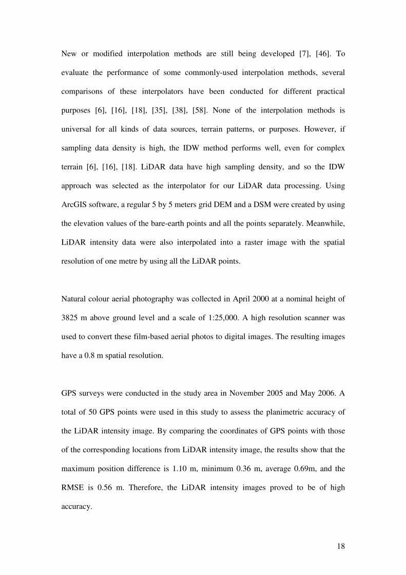
Natural colour aerial photography was collected in April 2000 at a nominal height of
3825 m above ground level and a scale of 1:25,000. A high resolution scanner was
used to convert these film-based aerial photos to digital images. The resulting images
have a 0.8 m spatial resolution.
GPS surveys were conducted in the study area in November 2005 and May 2006. A
total of 50 GPS points were used in this study to assess the planimetric accuracy of
the LiDAR intensity image. By comparing the coordinates of GPS points with those
of the corresponding locations from LiDAR intensity image, the results show that the
maximum position difference is 1.10 m, minimum 0.36 m, average 0.69m, and the
RMSE is 0.56 m. Therefore, the LiDAR intensity images proved to be of high
accuracy.

19
In order to assess the performance of proposed methodologies, especially to compare
with commonly used ground control data and DEMs for orthorectification, some of
the Vicmap datasets including Vicmap Elevation, Vicmap Transport, and Vicmap
Features datasets are also gathered. Vicmap is a set of spatially related data products
made up from individual datasets. They provide foundation to Victorian primary
mapping and geographic information systems. All these datasets are produced and
maintained by the Victorian Department of Sustainability and Environment, Australia.
Vicmap Elevation, a statewide 20 m resolution DEM which is structured in a regular
array of pixels representing Victoria’s terrain surface, is a commonly used elevation
data source in Victoria for various terrain-related applications and processes including
orthorectification. Vicmap DEM was produced by using elevation data mainly derived
from existing 1:25,000 contour maps and digital stereo capture. Estimated standard
deviations are 5m and 10m for vertical and horizontal accuracy respectively [21].
Vicmap Transport models transport infrastructure networks for Victoria. Primary
feature types in Vicmap Transport are road centrelines and railways. Vicmap Features
contains infrastructure features such as fence lines, utility lines and landmarks. From
the perspective of digital photogrammetric processing, road centrelines and fence
lines are the most interesting features for collecting GCPs. However, the accuracy of
these datasets should be noted when using them for the purpose of GCP collection.
The estimated standard deviation for these features is 8.2 m [22], [23]. It may be not
suitable for GCP collection for large scale aerial image orthorectification.
4.3. Method

20
Erdas Imagine 8.7 (a digital photogrammetric software package) is used to process
digital images from scanned aerial photographs. An example of these images used for
this study is shown in Figure 2. Features depicted include agricultural lands,
residential areas, roads, trees, and salt lakes. These raw digital perspective images are
the original input images to undergo block triangulation and orthorectification. The
subsequent steps are to enter the camera calibration data, measure the fiducial marks
on the images, and perform interior orientation parameters calculation for each image.
Figure 2. An example of scanned natural colour aerial photographs with highlighted
positions of GCPs measurements.
Following the interior orientation, it is ready to measure the positions of GCPs in the
images and provide their correspondent ground (or object space) coordinates for aerial
triangulation. The LiDAR intensity image has an orthogonal nature and is
georeferenced to the Geocentric Datum of Australia 94 (GDA94) and projected to the

21
MGA Zone 54 coordinate system so that it is much like a high accuracy large scale
topographic map. The LiDAR intensity image makes it much easier to identify
features such as road intersections and agricultural land plot boundaries, which are
commonly used as GCPs. Due to the high accuracy characteristics of LiDAR data, the
intensity image is well suited for providing ground control truth information for aerial
triangulation calculation. Therefore, the X and Y coordinates of GCPs in object space
can be directly collected from LiDAR intensity images; Z coordinates being obtained
from the LiDAR-derived DEM. An example of LiDAR intensity images used for this
study is shown in Figure 3, which covers the same area as the aerial image in Figure 2.
Highlighted marks represent the locations where the ground coordinates of GCPs
were picked up.
Figure 3. A LiDAR intensity image, which covers the same area as the scanned aerial
photograph in Figure 2.

22
Once the aerial triangulation process is complete, digital orthorectification can be
conducted. During this process, the raw digital imagery is resampled to the correct
ground position. The effects of terrain relief displacement are removed by utilizing a
LiDAR-derived high quality DEM.
With the aim of assessing the suitability of using GCPs derived from the LiDAR
intensity image for aerial triangulation and of using the LiDAR-derived DEM for
image orthorectification, the scanned aerial images same as above but using Vicmap
data for providing GCPs and DEM were input to the same digital photogrammetric
software for aerial triangulation and orthorectification. Here, the object space
coordinates of GCPs were obtained from Vicmap Transport and Vicmap Features.
The DEM was based on 20 m resolution Vicmap Elevation data. For the purpose of
comparison, the same object features were used for GCPs and the same number of
GCPs was picked up.
5. Results and discussion
Using the method described above, scanned natural colour aerial photographs were
orthorectified to the final orthoimages. GCPs and the DEM used for the
photogrammetric and orthorectification process were obtained from LiDAR data and
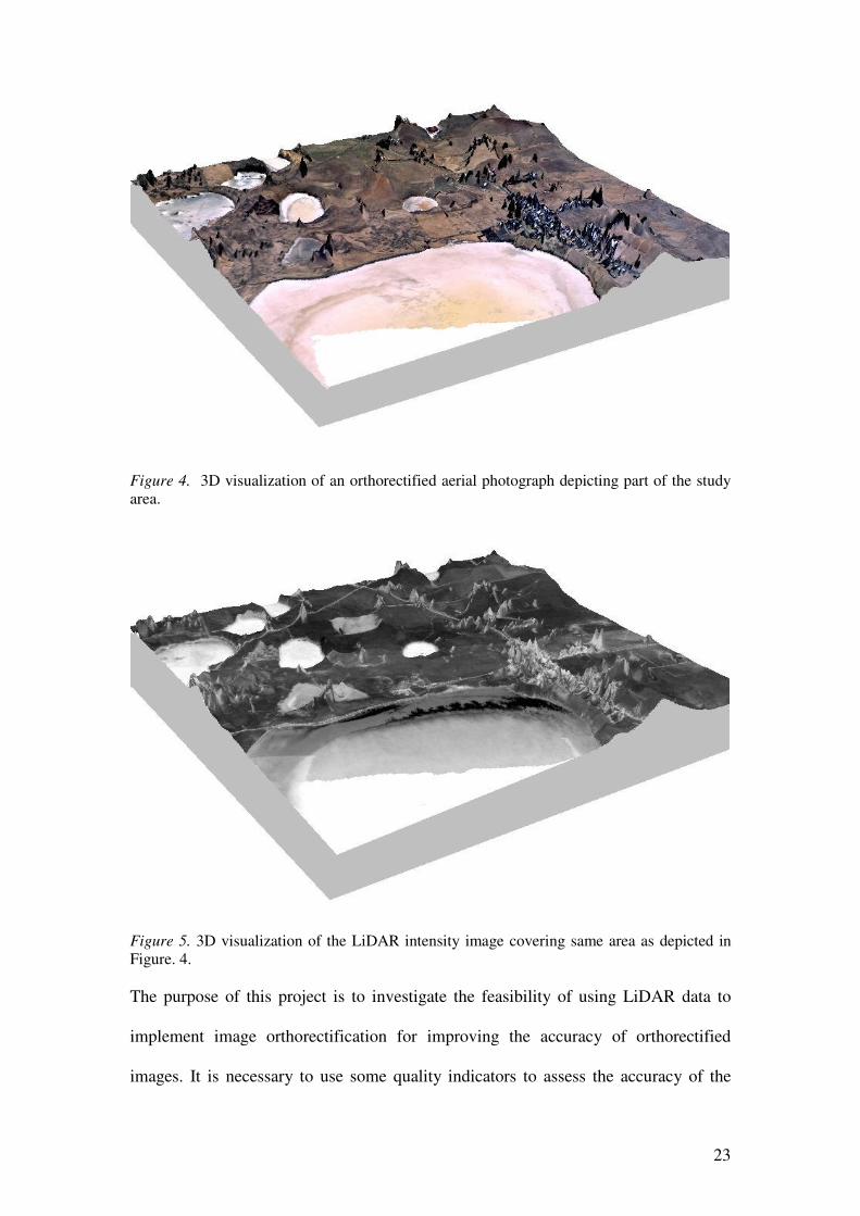
Vicmap data separately. An example of the orthorectified image by using LiDAR-
generated GCPs and DEM, draped on a LiDAR-derived digital surface model (DSM)
is shown in Figure. 4. The features on this orthoimage should be in their correct
positions. The reference LiDAR intensity image draped on terrain surface, covering
same area as in Figure 4 is shown in Figure 5.
23
Figure 4. 3D visualization of an orthorectified aerial photograph depicting part of the study
area.
Figure 5. 3D visualization of the LiDAR intensity image covering same area as depicted in
Figure. 4.
The purpose of this project is to investigate the feasibility of using LiDAR data to
implement image orthorectification for improving the accuracy of orthorectified
images. It is necessary to use some quality indicators to assess the accuracy of the

24
resulting orthoimages. For orthoimages, it is important to evaluate the planimetric
accuracy. The X and Y coordinates of check points in the orthoimage were measured,
and then compared with the corresponding coordinates from differential GPS surveys.
The planimetric position differences between orthoimages (orthorectified based on
LiDAR data on the one hand and Vicmap data on the other) and the GPS check points
are listed in Table 1. Based on these data, a statistic diagram was drawn in Figure. 6,
showing position differences of each check points for the image orthorectified using
LiDAR data, and for the image orthorectified using Vicmap data.
Table 1. Planimetric position accuracy.
Coordinates from
GPS Survey (I0)
(m)
Coordinates from
LiDAR-orthorectified
Image (I1) (m)
Coordinates from
Vicmap-orthorectified
Image (I2) (m)
Position
Difference
(m)
X Y X Y X Y |I1 - I0| |I2 - I0|
31761.84 67258.49 31762.11 67258.18 31759.93 67262.49 0.41 4.43
28414.79 69458.39 28415.61 69459.89 28408.02 69451.09 1.70 9.96
31037.51 68701.59 31037.87 68702.45 31036.01 68697.75 0.93 4.12
30929.38 68945.13 30929.68 68945.75 30929.75 68941.39 0.69 3.76
30811.17 69179.83 30811.37 69179.08 30809.47 69173.26 0.78 6.78
30946.31 69179.32 30946.86 69180.80 30944.89 69174.17 1.58 5.34
31079.91 69164.53 31079.79 69165.92 31078.41 69160.95 1.40 3.88
31058.73 68933.38 31058.82 68934.54 31057.69 68929.27 1.16 4.24
26961.03 67486.52 26961.47 67486.66 26957.27 67482.76 0.46 5.32
28207.44 68641.17 28207.27 68641.34 28200.98 68639.31 0.24 6.71
29092.21 71499.51 29091.44 71500.97 29080.72 71498.04 1.65 11.58
30845.77 69443.33 30846.16 69445.14 30852.78 69437.85 1.85 8.90
31114.13 70633.01 31114.04 70631.52 31110.87 70629.64 1.49 4.69
31029.86 70956.87 31030.13 70955.69 31027.14 70954.58 1.21 3.56
31152.02 68461.31 31152.28 68462.69 31151.08 68457.58 1.40 3.85
30147.19 72033.51 30147.43 72031.94 30136.48 72035.53 1.59 10.90
31026.37 68469.42 31026.81 68469.96 31025.49 68465.69 0.70 3.83
31211.47 69158.06 31212.29 69156.86 31209.59 69148.07 1.45 10.17
28396.05 70296.71 28396.59 70295.53 28389.80 70287.15 1.30 11.42
25757.33 67071.38 25756.67 67072.75 25756.05 67063.85 1.52 7.64
Table 1 and Figure 6 clearly indicate that the orthorectified image by using LiDAR-
derived GCPs and the LiDAR DEM has much higher planimetric position accuracy
than that by using Vicmap based data. The maximum position difference in the
LiDAR-orthorectified image is 1.85 m, while the difference is up to 11.58 m in

25
Vicmap-orthorectified image. By using the following formula, the root mean square
errors (RMSE) were calculated as 1.30 m for LiDAR-orthorectified orthoimage and
7.26 m for Vicmap-orthorectified orthoimage
Pσ =
1
2
−
∑∆
n
P
where, P∆ is the calculated position difference between the orthoimage and GPS
survey, and n is the total number of points.
0
2
4
6
8
10
12
Po
siti
on
Dif
fere
nce
(m
)
1 3 5 7 9 11 13 15 17 19
Point Number
Errors of LiDAR-Orthorectified Image
Errors of Vicmap-Orthorectified Image
Figure 6. Planimetric position accuracy
The planimetric position accuracy of an orthoimage is a function of the quality of the
input GCPs, DEM, and also some other factors. The accuracy of GCPs and the DEM
is reflected in the accuracy of the orthoimage. The experiment results demonstrated
that the competent use of LiDAR-based GCPs and LiDAR-derived DEM can ensure
high quality for orthorectification. Given the accuracy of LiDAR data used for this

26
project, a high accuracy of horizontal position for orthorectified images can certainly
be achieved. GCP coordinates acquired from LiDAR intensity image and the DEM
generated from LiDAR data are well suited for the orthorectification process of aerial
photography of medium and large scales.
LiDAR data do not only provide high accuracy GCPs and DEM for improving the
accuracy of an orthorectified image, they but also have great potential to reduce the
costs of orthorectification of aerial photography, especially for remote areas. With the
increasing availability and steadily decreasing cost of LiDAR data, it is becoming
common for remotely sensed overlaying datasets to include not only aerial
photography but LiDAR data also. It has attracted an increasing amount of interest to
explore these data’s complementary characteristics. The results lead to the potential
decrease of the costs of a specific traditional process, such as using LiDAR data to
support the orthorectification of aerial photography.
6. Conclusion
Different levels of image rectification and factors contributing to orthorectified
images were first addressed in this paper. Then it presented a way of using LiDAR-
derived GCPs and DEMs for image orthorectification. High accuracy LiDAR data
offer the capability of obtaining GCPs and DEMs at a higher level of accuracy
required for photogrammetric and orthorectification processes. The ground
coordinates of GCPs were obtained from LiDAR intensity map, while DEMs were
generated from high accuracy 3D LiDAR point clouds. The experiment results in this
paper demonstrated the practical feasibility of taking advantage of LiDAR based
GCPs and LiDAR-derived DEM in digital photogrammetry to produce high quality
orthorectified images. The orthoimage accuracy by using LiDAR data is superior to
27
that achieved by using lower accuracy data sources such as Vicmap. In addition to the
accuracy aspect, it is expected that using LiDAR data for orthorectification process
would be a cost effective way. This is especially true with the increasing availability
of LiDAR data and the expected drop in costs.
Acknowledgment
The authors would like to thank three anonymous reviewers for their valuable
comments and suggestions. We are also grateful to the Corangamite Catchment
Management Authority for providing LiDAR data and other datasets to support this
project.
References
1. AAMHatch. Corangamite CMA airborne laser survey data documentation,
AAMHatch Pty Ltd, Melbourne, Australia, 2003.
2. Y. B. Acharya, S. Sharma and H. Chandra. "Signal induced noise in PMT
detection of lidar signals", Measurement, Vol. 35(3):269-276, 2004.
3. F. Ackermann. "Airborne laser scanning - present status and future
expectations", ISPRS Journal of Photogrammetry and Remote Sensing, Vol.
54(4):64-67, 1999.
4. F. Ackermann and P. Krzystek. "Complete automation of digital aerial
triangulation", Photogrammetric Record, Vol. 15(89):645-656, 1997.
5. S. Ahlberg, U. Söderman, M. Elmqvist and A. Persson. "On modelling and
visualisation of high resolution virtual environments using lidar data", in
Proceedings of 12th International Conference on Geoinformatics, Gävle,
Sweden, 2004. pp.299-306.

28
6. T. A. Ali. "On the selection of an interpolation method for creating a terrain
model (TM) from LIDAR data", in Proceeding of the American Congress on
Surveying and Mapping (ACSM) Conference 2004, Nashville TN, U.S.A,
2004.
7. A. Almansa, F. Cao, Y. Gousseau and B. Rougé. "Interpolation of digital
elevation models using amle and related methods", IEEE Transactions on
Geoscience and Remote Sensing, Vol. 40(2):314-325, 2002.
8. F. Amhar, J. Jansa and C. Ries. "The generation of true orthophotos using a
3D building model in conjunction with a conventional DTM", International
Archives of the Photogrammetry, Remote Sensing and Spatial Information
Sciences, Vol. 32(Part 4):16-22, 1998.
9. N. S. Arnold, W. G. Rees, B. J. Devereux and G. S. Amable. "Evaluating the
potential of high-resolution airborne LiDAR data in glaciology", International
Journal of Remote Sensing, Vol. 27(6):1233-1251, 2006.
10. E. Baltsavias and R. Bill. "Scanners - a survey of current technology and
future needs ", International Archives of the Photogrammetry, Remote Sensing
and Spatial Information Sciences, Vol. 30(Part 1):130-143, 1994.
11. E. P. Baltsavias. "Photogrammetric scanners - survey, technological
developments and requirements", International Archives of the
Photogrammetry, Remote Sensing and Spatial Information Sciences, Vol.
32(Part 1):44-52, 1998.
12. E. P. Baltsavias. "A comparison between photogrammetry and laser scanning",
ISPRS Journal of Photogrammetry and Remote Sensing, Vol. 54(4):83-89,
1999.

29
13. E. P. Baltsavias, E. Favey, A. Bauder and H. Bosch. "Digital surface
modelling by airborne laser scanning and digital photogrammetry for glacier
monitoring", Photogrammetric Record, Vol. 17(98):243-273, 2001.
14. M. Barbarella, V. Lenzi and M. Zanni. "Integration of airborne laser data and
high resolution satellite images over landslides risk areas", International
Archives of the Photogrammetry, Remote Sensing and Spatial Information
Sciences, Vol. 35(B4):945-950, 2004.
15. C. P. Barber and A. M. Shortrudge. Light Detection and Ranging (LiDAR)-
derived elevation data for surface hydrology applications, Institute of Water
Resource, Michigan State University, USA, 2004.
16. T. Blaschke, D. Tiede and M. Heurich. "3D landscape metrics to modelling
forest structure and diversity based on laser scanning data", International
Archives of the Photogrammetry, Remote Sensing and Spatial Information
Sciences, Vol. 36(8/W2):129-132, 2004.
17. E. V. Browell, W. B. Grant and S. Ismail. "Airborne LiDAR system", in T.
Fujii and T. Fukuchi (Eds.), Laser Remote Sensing, Taylor & Francis: Boca
Raton, London, New York and Singapore, pp. 723-779, 2005.
18. V. Chaplot, F. Darboux, H. Bourennane, S. Leguédois, N. Silvera and K.
Phachomphon. "Accuracy of interpolation techniques for the derivation of
digital elevation models in relation to landform types and data density",
Geomorphology, Vol. 77(1-2):126-141, 2006.
19. A. P. Charaniya, R. Manduchi and S. K. Lodha. "Supervised parametric
classification of aerial LiDAR data ", in Proceedings of 2004 Conference on
Computer Vision and Pattern Recognition Workshop (CVPRW'04),
Washington D.C, USA, 2004.
30
20. F. Coren, D. Visintini, G. Prearo and P. Sterzai. "Integrating LiDAR intensity
measures and hyperspectral data for extracting of cultural heritage", in
Proceedings of Italy - Canada 2005 Workshop on 3D Digital Imaging and
Modeling: Applications of Heritage, Industry, Medicine and Land, Padova,
Italy, 2005.
21. DSE. Product Description - Vicmap Elevation, Department of Sustainability
and Environment, Victoria, Australia, 2002.
22. DSE. Product Description - Vicmap Features, Department of Sustainability
and Environment, Victoria, Australia, 2005.
23. DSE. Product Description - Vicmap Transport, Department of Sustainability
and Environment, Victoria, Australia, 2005.
24. Leica Geosystems. Leica photogrammetry suite orthoBASE & orthoBASE Pro
user's guide, Leica Geosystems GIS & Mapping, LLC, Atlanta, Georgia, USA,
2003.
25. A. Habib, M. Ghanma, M. Morgan and R. Al-Ruzouq. "Photogrammetric and
LiDAR data registration using linear features", Photogrammetric Engineering
and Remote Sensing, Vol. 71(6):699-707, 2005.
26. A. F. Habib, M. S. Ghanma, C. J. Kim and E. Mitishita. "Alternative
approaches for utilizing LiDAR as a source of control information for
photogrammetric models", International Archives of the Photogrammetry,
Remote Sensing and Spatial Information Sciences, Vol. 35(B1):193-198, 2004.
27. M. Hollaus, W. Wagner and K. Kraus. "Airborne laser scanning and
usefulness for hydrological models", Advances in Geosciences, Vol. 5(1):57-
63, 2005.
28. A. V. Jelalian. Laser Radar Systems, Artech House: Boston and London, 1992.

31
29. S. Kaasalainen, E. Ahokas, J. Hyyppä and J. Suomalainen. "Study of surface
brightness from backscattered laser intensity: calibration of laser data", IEEE
Geoscience and Remote Sensing Letters, Vol. 2(3):255-259, 2005.
30. M. Kasser and Y. Egels. Digital Photogrammetry, Taylor and Francis: London
and New York, 2002.
31. A. Krupnik. "Accuracy prediction for ortho-image generation",
Photogrammetric Record, Vol. 18(101):41-58, 2003.
32. D. Li, J. Gong, Y. Guan and C. Zhang. "Accuracy analysis of digital
orthophotos", International Archives of the Photogrammetry, Remote Sensing
and Spatial Information Sciences, Vol. 36(W20):241-244, 2002.
33. X. Liu, J. Peterson and Z. Zhang. "High-resolution DEM generated from
LiDAR data for water resource management", in Proceedings of International
Congress on Modelling and Simulation 'MODSIM05', Melbourne, Australia,
2005. pp.1402-1408.
34. X. Liu, J. Peterson, Z. Zhang and S. Chandra. "Improving soil salinity
prediction with high resolution DEM derived from LiDAR data", International
Archives of the Photogrammetry, Remote Sensing and Spatial Information
Sciences, Vol. 36(7/W20):41-43, 2005.
35. C. D. Lloyd and P. M. Atkinson. "Deriving ground surface digital elevation
models from LiDAR data with geostatistics", International Journal of
Geographical Information Science, Vol. 20(5):535-563, 2006.
36. J. L. Lovell, D. L. B. Jupp, D. S. Culvenor and N. C. Coops. "Using airborne
and ground-based ranging lidar to measure canopy structure in Australian
forests", Canadian Journal of Remote Sensing, Vol. 29(5):606-622, 2003.

32
37. A. Macke and M. Groβklaus. "Light scattering by nospherical raindrops:
implications for LiDAR remote sensing of rainrates ", Journal of Quantitative
Spectroscopy & Radiative Transfer, Vol. 60(3):355-363, 1998.
38. M. G. Mardikis, D. P. Kalivas and V. J. Kollias. "Comparison of interpolation
methods for the prediction of reference evapotranspiration - an application in
Greece", Water Resources Management, Vol. 19(3):251-278, 2005.
39. G. Méjean, J. Kasparian, E. Salmon, J. Yu, J. P. Wolf, R. Bourayou, R.
Sauerbrey, M. Rodriguez, L. Wöste, H. Lehmann, B. Stecklum, U. Laux, J.
Eislöffel, A. Scholz and A. P. Hatzes. "Towards a supercontinuum-based
infrared lidar", Applied Physics B: Lasers and Optics, Vol. 77(2-3):357-359,
2003.
40. T. Moffiet, K. Mengersen, C. Witte, R. King and R. Denham. "Airborne laser
scanning: exploratory data analysis indicates potential variables for
classification of individual trees or forest stands according to species", ISPRS
Journal of Photogrammetry and Remote Sensing, Vol. 59(5):289-309, 2005.
41. T. Mukai, A. M. Nakamura and T. Sakai. "Asteroidal surface studies by
laboratory light scattering and LIDAR on HAYABUSA", Advances in Space
Research, Vol. 37(1):138-141, 2006.
42. J. A. Parian and A. Gruen. "Integrated laser scanner and intensity image
calibration and accuracy assessment", International Archives of the
Photogrammetry, Remote Sensing and Spatial Information Sciences, Vol.
36(3/W19):18-23, 2005.
43. C. E. Parrish, G. H. Tuell, W. E. Carter and R. L. Shrestha. "Configuring an
airborne laser scanner for detecting airport obstructions", Photogrammetric
Engineering and Remote Sensing, Vol. 71(1):37-46, 2005.

33
44. S. E. Reutebuch, H. E. Andersen and R. J. McGaughey. "Light detection and
ranging (LIDAR): an emerging tool for multiple resource inventory", Journal
of Forestry, Vol. 103(6):286-292, 2005.
45. Y. Sheng, P. Gong and G. S. Biging. "Orthoimage production for forested
areas from large-scale aerial photographs", Photogrammetric Engineering and
Remote Sensing, Vol. 69(3):259-266, 2003.
46. W. Z. Shi and Y. Tian. "A hybrid interpolation method for the refinement of a
regular grid digital elevation model", International Journal of Geographical
Information Science, Vol. 20(1):53-67, 2006.
47. J. H. Song, S. H. Han, K. Yu and Y. I. Kim. "Assessing the possibility of land-
cover classification using lidar intensity data", International Archives of the
Photogrammetry, Remote Sensing and Spatial Information Sciences, Vol.
34(Part 3A):259-262, 2002.
48. W. Wagner, A. Ullrich, T. Melzer, C. Briese and K. Kraus. "From single-pulse
to full-waveform airborne laser scanners: potential and practical challenges",
International Archives of the Photogrammetry, Remote Sensing and Spatial
Information Sciences, Vol. 35(B3), 2004.
49. A. S. Walker. "Responses to users: the continuing evolution of commercial
digital photogrammetry", Photogrammetric Record, Vol. 16(93):469-483,
1999.
50. D. Watkins. LiDAR types and uses: with a case study in forestry, Department
of Geography, Pennsylvania State University, USA, 2005.
51. T. L. Webster and G. Dias. "An automated GIS procedure for comparing GPS
and proximal LiDAR elevations", Computers & Geosciences, Vol. 32(6):713-
726, 2006.

34
52. A. Wehr and U. Lohr. "Airborne laser scanning - an introduction and overview
", ISPRS Journal of Photogrammetry and Remote Sensing, Vol. 54(4):68-82,
1999.
53. C. Weitkamp. "LiDAR: Introduction", in T. Fujii and T. Fukuchi (Eds.), Laser
Remote Sensing, Taylor & Francis: Boca Raton, London, New York and
Singapore, pp. 1-36, 2005.
54. R. Welch and T. Jordan. "Using scanned aerial photographs", in S. Morain and
S. L. Baros (Eds.), Raster Imagery in Geographic Information Systems,
OnWord Press: Santa Fe, NM, USA, pp. 55-69, 1996.
55. K. Q. Zhang, S. C. Chen, D. Whitman, M. L. Shyu, J. H. Yan and C. C. Zhang.
"A progressive morphological filter for removing nonground measearements
from airborne LiDAR data", IEEE Transactions on Geoscience and Remote
Sensing, Vol. 41(4):872-882, 2003.
56. G. Zhou, W. Chen, J. A. kelmelis and D. Zhang. "A comprehensive study on
urban true orthorectification", IEEE Transactions on Geoscience and Remote
Sensing, Vol. 43(9):3138-2147, 2005.
57. G. Zhou, W. Schichler, A. Thorpe, P. Song, W. Chen and C. Song. "True
orthoimage generation in urban areas with very tall buildings", International
Journal of Remote Sensing, Vol. 25(22):5163-5180, 2004.
58. D. Zimmerman, C. Pavlik, A. Ruggles and M. P. Armstrong. "An
experimental comparison of ordinary and universal Kriging and inverse
distance weighting", Mathematical Geology, Vol. 31(4):375-389, 1999.