USDOTRegionVRegionalUniversityTransportationCenterFinalReport

IL IN

WI

MN

MI

OH

NEXTRANSProjectNo.123OSUY2.1

LIDARBasedVehicleClassification

By

BenjaminCoifman,PhDAssociateProfessor

TheOhioStateUniversityDepartmentofCivil,Environmental,andGeodeticEngineering

DepartmentofElectricalandComputerEngineeringHitchcockHall470

2070NeilAve,Columbus,OH43210E-mail:Coifman.1@OSU.edu

and

HoLeeTheKoreaTransportInstitute

DepartmentofRailwayResearch

DISCLAIMER

Funding for this research was provided by the NEXTRANS Center, Purdue University underGrantNo.DTRT12-G-UTC05of theU.S.DepartmentofTransportation,Officeof theAssistantSecretary for Research and Technology (OST-R), University Transportation Centers Program.Thecontentsofthisreportreflecttheviewsoftheauthors,whoareresponsibleforthefactsand the accuracyof the informationpresentedherein. This document is disseminatedunderthe sponsorship of the Department of Transportation, University Transportation CentersProgram,intheinterestofinformationexchange.TheU.S.Governmentassumesnoliabilityforthecontentsorusethereof.

INTRODUCTION

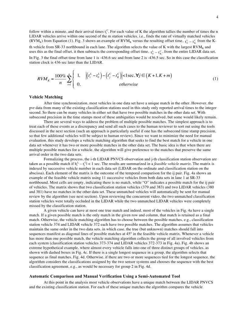
Vehicle classification data are used in many transportation applications, including: pavement design, environmental impact studies, traffic control, and traffic safety (FHWA, 2001). There are several classification methods, including: axle-based (e.g., pneumatic tube and piezoelectric detectors), vehicle length-based (e.g., dual loop and some wayside microwave detectors), as well as emerging machine vision based detection. Each sensor technology has its own strengths and weaknesses regarding costs, performance, and ease of use.

Operating agencies spend millions of dollars to deploy vehicle classification stations to collect classified count data, yet very few of these stations are ever subjected to a rigorous performance evaluation to ensure that they are reporting accurate data. As noted in the Traffic Monitoring Guide (FHWA, 2001), the quality of data collected depends on the operating agency to periodically calibrate, test, and validate the performance of classification sensors, but few operating agencies have an on-going performance monitoring system to ensure that well tuned classification stations do not drift out of tune. Both one time and periodic performance monitoring have been prohibitively labor intensive because the only option has been to manually validate the performance, e.g., classifying a sample by hand. When these studies are conducted, the manual classifications are usually of limited value both because the manual data are prone to human error, and among the few studies that have been published, most employ the conventional reporting periods used by the stations (typically 15 min periods or longer), which are too coarse, allowing over-counting errors to cancel under-counting errors.

In the present study we develop a classification performance monitoring system to allow operating agencies to rapidly assess the performance of existing classification stations on a per vehicle basis. We eliminate most of the labor demands and instead, deploy a portable non-intrusive vehicle classification system (PNVCS) to classify vehicles, concurrent with an existing classification station. For this study we use a side-fire LIDAR (light detection and ranging) based classifier from Lee and Coifman (2012a) for the PNVCS. Fig. 1 shows a flowchart of our performance evaluation system. The existing classification station normally follows the three boxes within the dashed region (top left of the figure) when it is not under evaluation. The PNVCS is shown immediately to the right of the dashed region. To prevent classification errors from canceling one another in aggregate, we record per-vehicle record (pvr) data in the field from both systems. After the field collection the classification results are evaluated on a per-vehicle basis. Algorithms for time synchronization and for matching observations of a given vehicle between the two classification systems are developed in this study. These algorithms automatically compare the vehicle classification between the existing classification station and the PNVCS for each vehicle. If the two systems agree, the given vehicle is automatically taken as a success by the classification station under the implicit assumptions: (i) That few vehicles will be misclassified the same way by the two independent classification systems. (ii) That the PNVCS has sufficient accuracy so that its data can be used as a benchmark for the existing classification station (in this case Lee and Coifman, 2012a, found that the LIDAR system classified vehicles with 99.5% accuracy on an evaluation set of 21,769 non-occluded vehicles).

The temporary deployment includes a video camera mounted close to the LIDAR sensors and pointed at their detection zone (right-most path in Fig. 1) to allow a human to assess any discrepancies. A human only looks at a given vehicle when the two systems disagree, and for this task we have developed tools to semi-automate the manual validation process, greatly increasing the efficiency and accuracy of the human user. The data sets in this study take only a few minutes for the user to validate an hour of pvr data from a multi-lane facility.

Although we use a LIDAR based system in this study, the tools at the heart of the methodology are transferable to many PNVCS from conventional pneumatic tubes to emerging PNVCS such as the TIRTL by Control Specialists, AxleLight by Quixote, the prototype ORADS (more recently NTMS) by Spectra Research (CEOS, 2012; Peek Traffic, 2010; Little et al., 2001; Spectra Research, 2011). These emerging PNVCS were specifically developed to replace pneumatic tubes and use light beams just above the pavement to implement axle-based classification. The TIRTL performed very well at measuring axle spacing on two lane highways, typically above 95% accuracy (Yu et al., 2010), though some studies found an error rate of 24% among the truck classes due to the default decision tree (Kotzenmacher et al., 2005; Minge, 2010; Minge et al., 2011). While the AxleLight had an error rate for the truck classes up to 34% in high volume across four lanes (Minge, 2010; Minge et al., 2011; Banks, 2008), which was attributed to the sensor mistaking closely-following two-axle vehicles for multi-axle trucks. Most of the errors in Minge (2010) and Minge et al. (2011) were corrected by post-processing the pvr data from AxleLight and TIRTL using a new decision tree. Meanwhile, other studies found the TIRTL performance degrades on four lane roads (French and French, 2006). Finally, commercial side-fire microwave radar systems do not currently appear to offer sufficient classification accuracy to be used for this application. Even allowing the

2

individual errors to cancel in aggregate data, the SmartSensor had an overall error rate for trucks of 46% (Kotzenmacher et al., 2005), 80% (Zwahlen et al, 2005), 50%-400% (French and French, 2006), 20%-50% (Yu et al., 2010) and the RTMS had an error rate for trucks of 25% (Kotzenmacher et al., 2005) and 40%-97% (French and French, 2006). While most of the previous studies used aggregate data, two studies used a small sample of pvr data, only a few hundred vehicles, and found the SmartSensor had an error rate for trucks of 13%-57% (Banks, 2008) and 42% (Minge, 2010). A few studies considered video systems, e.g., Yu et al. (2010) found the length based classification from an Autoscope to be unacceptable, while Schwach et al. (2009) had an error rate for trucks of 73%.

The primary objective of this study is to demonstrate the viability of our methodology to use a PNVCS to evaluate the performance of an existing vehicle classification station, regardless of the PNVCS technology used. A secondary objective of this study is to demonstrate that the LIDAR based PNVCS from Lee and Coifman (2012a) indeed offers the required accuracy. The remainder of this report is organized as follows. First the process of collecting the concurrent pvr vehicle classification data from the LIDAR and existing classification station is presented. Second, the performance evaluation methodology is developed. Third, the methodology is applied to several permanent and temporary vehicle classification stations to evaluate axle and length-based classification. The evaluation data sets include over 21,000 vehicles, less than 8% of which required manual intervention. Finally, the report closes with a discussion and conclusions.

METHODOLOGY OF USING A PNVCS TO EVALUATE CLASSIFICATION STATION PERFORMANCE

This section develops the semi-automated performance evaluation methodology for an existing classification station using LIDAR PNVCS classification, as shown in Fig. 1. This section begins by reviewing the key features of the LIDAR based PNVCS. Then, it discusses the four key steps for the performance evaluation: first the input classification data itself, second the time synchronization algorithm, third the vehicle matching algorithm to match observations of a given vehicle between the two classification systems, and fourth the semi-automated tool to allow a human to rapidly review any discrepancies between the two classification systems. The discrepancies include both conflicting classifications and vehicles seen by just one of the systems. In the absence of a discrepancy, a vehicle is automatically recorded as a successful classification, without human intervention.

A Brief Review of the LIDAR based PNVCS This pilot study uses a LIDAR based PNVCS mounted on a van, as shown in Fig. 2c This van mounted

approach offers a distinct advantage over the other emerging PNVCS since the system does not require any calibration in the field, in fact the van can be classifying vehicles as it pulls up to the site. The LIDAR based PNVCS consists of a pair of Sick LMS 291-S05 scanning laser rangefinders, acting as vertical planar scanners, mounted as high as possible (approximately 2.2 m above ground) on the drivers side of the van in order to observe multiple adjacent lanes of traffic while minimizing occlusions. These LIDAR sensors were mounted with a separation of 1.4 m. They scan 180° of a vertical plane returning the distance to the nearest object (if any) at 0.5° increments with a maximum range of 80 m, at an update rate of approximately 37 Hz. Nonetheless, given the relatively low mounting location of the LIDAR sensors used in this study, vehicles in further lanes are susceptible to occlusions from vehicles in closer lanes. Using the same data set as used in the present study, Lee and Coifman (2012a) found roughly 11% of the vehicles were partially occluded and another 3% were totally occluded. Partial occlusions degrade the LIDAR classification performance, but the LIDAR classifier can automatically detect when a partial occlusion occurs. These vehicles are counted to ensure both detectors saw a single vehicle pass, but for now the classifications are not used since a partial occlusion in the LIDAR should not be correlated with misclassifications by the existing station. If simply setting the partially occluded vehicles aside like this is unacceptable for a given application, then Lee and Coifman (2012a) presents a means to classify them to one or more classes. They reported that roughly 50% of the partially occluded vehicles were assigned to a single class and could be processed automatically by the vehicle matching algorithm. The rest could be treated as a discrepancy and subjected to human evaluation with the semi-automated tool, thus, slightly increasing the number of vehicles sent for human assessment. For longer-term deployments we envision a dedicated trailer that could be parked alongside the road, with a boom to achieve a higher vantage point to reduce occlusions.

Totally occluded vehicles will only be recorded in the classification station data, resulting in a discrepancy. This pilot study mounted the camera close to the LIDAR sensors, so for most cases in our data the occluded vehicles

3

cannot be manually verified. Like the partially occluded vehicles, any systematic errors present in the totally occluded vehicles should also be evident in the non-occluded vehicles, and so the simplest solution is to collect a slightly larger data set to accommodate the fact that some vehicles will be occluded. Unlike the partially occluded vehicles, however, the risk remains that an unobserved actuation arose from splashover rather than an actual vehicle. Fortunately, the presence of chronic splashover can be detected automatically from the classification station data using Lee and Coifman (2012b). Although the number of total occlusions was small in our study, many simple steps can be used to further reduce the number including:

• mounting the LIDAR on a boom for a higher vantage point, • deploying a second camera on the far side of the roadway to supplement the manual evaluation, or • splitting the data collection into two sets- (1) with the LIDAR PNVCS deployed on the near side of the

roadway and then (2) deployed on the far side of the roadway. Thereby ensuring that if the station exhibits chronic splashover problems, in at least half of the data it will be towards the LIDAR PNVCS and thus, will be unoccluded.

The Classification Data Fig. 2a shows a hypothetical example of the time-space plane as a vehicle passes by the two LIDAR

sensors and Fig. 2b shows the corresponding schematic at an instant, using the same distance scale. The vertical scanning LIDAR capture the profile of the passing vehicles and spatial offset between the paired sensors allows for speed measurements. We use Lee and Coifman (2012a) to classify vehicles from the LIDAR data. Briefly summarizing the process: first we segment a given vehicle's LIDAR returns from the background, group the returns together into a cluster, look for possible occlusions in further lanes, and then we measure several features of size and shape for each non-occluded vehicle cluster. The algorithm uses these features to classify the vehicle clusters into six vehicle classes: motorcycle (MC), passenger vehicle (PV), PV pulling a trailer (PVPT), single unit truck/bus (SUT), SUT pulling a trailer (SUTPT), and multiple unit truck (MUT). For this study PVPT are included with PV and SUTPT are included with MUT, following common axle-based classification conventions (Lee and Coifman, 2012b).

In the present study of existing classification stations we evaluate both axle-based classification and length-based classification. We evaluate two permanent vehicle classification stations (total of three directional stations) each equipped with dual loop detectors and a piezoelectric sensor in each lane and two temporary vehicle classification deployments (total of four directional stations) with pneumatic tubes. All of these existing classification stations provide the conventional 13 axle-based classes and this research consolidates them into four classes to facilitate comparison with the LIDAR PNVCS, i.e., axle class 1 is mapped to MC, axle class 2-3 are mapped to PV, axle class 4-7 are mapped to SUT, and axle class 8-13 are mapped to MUT. The permanent vehicle classification stations also provide length-based vehicle classification with three length-classes that are intended to map to PV, SUT and MUT, respectively. Finally, we also tested the system at a single loop detector station deployed for real time traffic monitoring using Coifman and Kim (2009) for length-based classification. All of the data sets were collected in the Columbus, Ohio, metropolitan area.

Time Synchronization The LIDAR PNVCS and the existing classification station clocks are independent, so before any

comparisons are made it is necessary to first find the offset between the two systems. The algorithm has to accommodate the fact that any given vehicle may be seen in just one data set or the other due to detection errors and LIDAR occlusions. Our group has previously addressed a more complicated variant of this same problem for vehicle reidentification (Coifman and Cassidy, 2002), in which not only may a given vehicle be seen in just one of the data sets, but also vehicles will arrive in a different order in the two data sets. The updated algorithm is presented below. While the earlier vehicle reidentification had to address the reordering problem, in the current time synchronization problem the two locations are concurrent in space, so in this revision we use the arrival order to greatly simplify the problem of coordinating the two data sets.

The algorithm currently uses arrivals in one lane, over one minute, though we envision that expanding to multiple lanes or longer duration would improve the precision in challenging conditions. We arbitrarily select one vehicle in the LIDAR data as the reference (0-th vehicle), examine all n vehicles that follow within a minute, and record their arrival times, ti

L. The only constraint is that there must be concurrent data from the classification station. We then step through the station's vehicles from the same lane, successively taking each one as the station's reference (K-th vehicle, with arrival time C

Kt ) to test the assumption that CK

L0 tt = by evaluating all m vehicles that

4

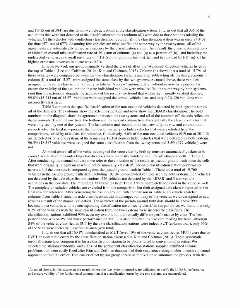
follow within a minute, and their arrival times tjC. For each value of K the algorithm tallies the number of times the n

LIDAR vehicles arrive within one second of the m station vehicles, i.e., finds the rate of virtually matched vehicles (RVMK) from Equation (1). Fig. 3 shows an example of RVMK versus the resulting offset time, C

KL0 tt - from the K-

th vehicle from SR-33 northbound in each lane. The algorithm selects the value of K with the largest RVMK and uses this as the final offset, it then subtracts the corresponding offset time, C

KL0 tt - , from the entire LIDAR data set.

In Fig. 3 the final offset time from lane 1 is -436.6 sec and from lane 2 is -436.5 sec. So in this case the classification station clock is 436 sec later than the LIDAR.

RVMK =100%n

1, tiL − t0

L( )− t jC − tK

C( ) <1sec,∀j ∈ K +1,K +m( )0, otherwise

$

%&

'&i=1

n

∑ (1)

Vehicle Matching After time synchronization, most vehicles in one data set have a unique match in the other. However, the

pvr data from many of the existing classification stations used in this study only reported arrival times to the integer second. So there can be many vehicles in either set that have two possible matches in the other data set. With subsecond precision in the time stamps most of these ambiguities would be resolved, but some would likely remain.

There are several ways to address the problem of multiple possible matches. The simplest approach is to treat each of these events as a discrepancy and send all such cases to the human reviewer to sort out using the tools discussed in the next section (such an approach is particularly useful if one has the subsecond time stamp precision, so that few additional vehicles will be subject to human review). Since we want to minimize the need for manual evaluation, this study develops a vehicle matching algorithm that seeks to find the best match for a vehicle in one data set whenever it has two or more possible matches in the other data set. The basic idea is that when there are multiple possible matches for a vehicle, the algorithm will give preference to the matches that preserve the same arrival order in the two data sets.

Formalizing the process, the i-th LIDAR PNVCS observation and j-th classification station observation are taken as a possible match if |ti

L – tjC| < 1 sec. The results are summarized in a feasible vehicle matrix. The matrix is

indexed by successive vehicle number in each data set (LIDAR on the ordinate and classification station on the abscissa). Each element of the matrix is the outcome of the temporal comparison for the ij pair. Fig. 4a shows an example of the feasible vehicle matrix using 11 successive vehicles from both data sets in lane 1 at SR-33 northbound. Most cells are empty, indicating there is no match, while “O” indicates a possible match for the ij pair of vehicles. The matrix shows that two classification station vehicles (379 and 383) and two LIDAR vehicles (380 and 381) have no matches in the other data set. These unmatched vehicles will automatically be sent for manual review by the algorithm (see next section). Upon reviewing the concurrent video, the two unmatched classification station vehicles were totally occluded in the LIDAR while the two unmatched LIDAR vehicles were completely missed by the classification station.

A given vehicle can have at most one true match and indeed, most of the vehicles in Fig. 4a have a single match. If a given possible match is the only match in the given row and column, that match is retained as a final match. Otherwise, the vehicle matching algorithm has to choose between the possible matches, e.g., classification station vehicle 374 and LIDAR vehicle 372 each have two possible matches. The algorithm assumes that vehicles maintain the same order in the two data sets, in which case, the true (but unknown) matches should fall into sequences manifest as diagonal lines of possible matches at 45° in the feasible vehicle matrix. Whenever a vehicle has more than one possible match, the vehicle matching algorithm collects the group of all involved vehicles from each system (classification station vehicles 373-374 and LIDAR vehicles 372-373 in Fig. 4a). Fig. 4b shows an extreme hypothetical example, where almost every vehicle falls into one of three distinct groups of vehicles, as shown with dashed boxes in Fig. 4c. If there is a single longest sequence in a group, the algorithm selects that sequence as final matches, Fig. 4d. Otherwise, if there are two or more sequences tied for the longest sequence, the algorithm considers the classifications assigned by the two sensor systems and chooses the sequence with the best classification agreement, e.g., as would be necessary for group 2 in Fig. 4d.

Automatic Comparison and Manual Verification Using a Semi-Automated Tool At this point in the analysis most vehicle observations have a unique match between the LIDAR PNVCS

and the existing classification station. For each of these unique matches the algorithm compares the vehicle

5

classification from the two independent systems and if the systems agree (e.g., both systems report PV for a given unique match) the vehicle is taken as a success by the classification station with no human intervention. The small number of vehicle observations that remain are then marked for manual evaluation. These marked vehicles consist of the vehicles that were seen in only one of the data sets (thus having no match in the other data set) and the unique matches where the two systems disagree (e.g., one reports PV and the other reports SUT).

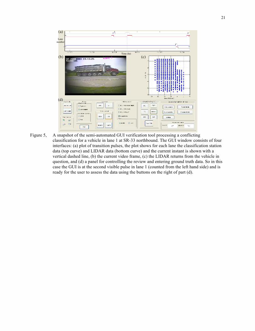
Inspired by VideoSync (Caltrans, 2007), a purpose built software ground truthing tool with a graphical user interface (GUI) was developed in MATLAB to efficiently review the vehicles marked for manual evaluation and increase the accuracy of the human user. After the time synchronization and vehicle matching steps above, the GUI loads the pvr classifications from the classification station and the LIDAR PNVCS. The user can choose which set(s) of vehicles they wish to review: (i) seen only in LIDAR, (ii) seen only at the classification station, (iii) conflicting classifications between the two sources, and/or (iv) consistent classification between the two sources. Normally the user would select the three error conditions, i.e., sets i-iii.1 Next, the user chooses one or more lanes to review, then the GUI steps through all of the vehicles in the given set(s) and lane(s). Fig. 5 shows an example of the GUI as a SUT passes. For each vehicle the GUI displays the raw LIDAR data and the raw classification station data for a few seconds before and after the given vehicle detection (Figs. 5c and 5a, respectively). The GUI shows the video frame at the instant of the vehicle passage (Fig. 5b), and allows the user to step forward or backward in the video to see the temporal evolution if necessary (Fig. 5d). The bottom right corner of the GUI shows the user what vehicle class was assigned by the station and the LIDAR. After assessing the concurrent sensor and video data, the user records the observed vehicle class or detection error for the current actuation using the buttons in the two right-most boxes of Fig. 5d. As soon as the user enters a selection, the GUI jumps to the next actuation in the selected set(s) and lane(s) until all of the vehicles have been reviewed in the given set(s) from the entire time period with video data. In this study the user typically spent 3-5 sec per vehicle reviewed (including seek time and loading time), but only about 8% of the actuations required review. The automated process does the bulk of the work, in this study it typically took the human only a few minutes to process the exceptions from all lanes over one hour of data.

RESULTS OF USING A PNVCS TO EVALUATE CLASSIFICATION STATION PERFORMANCE

Axle-Based Classification Stations As noted above, we collected concurrent LIDAR and axle classification station pvr data at two permanent

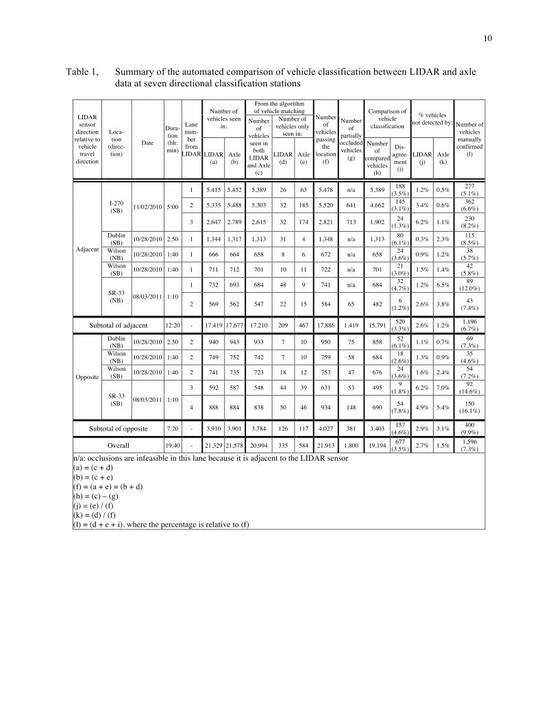
vehicle classification stations (I-270 and SR-33) and two temporary deployments (Wilson Rd and Dublin Rd). Table 1 enumerates the location, date, duration, and number of lanes in the first few columns. All locations yielded data for the direction of travel adjacent to the LIDAR equipped van (top rows in the table). Almost all of the locations provided sufficient view of the far lanes in the opposing direction to allow LIDAR classification, shown in the lower portion of the table. The one exception was I-270, where the median barrier and superelevation precluded a view of the opposing lanes. In any event, all lanes are numbered successively from the van, regardless of the direction of travel. We parked the van on both sides of Wilson Rd, hence both northbound and southbound nearside data for this location.

Columns (a) and (b) show the number of actuations reported by the LIDAR and classification data (including any non-vehicle actuations). Columns (c)-(e) show the number of matched and unmatched actuations after the vehicle matching algorithm. Column (f) sums columns (c), (d), and (e), yielding the number of actuations seen by one or both systems. Column (g) tallies the number of partially occluded vehicles detected in the LIDAR (as per Lee and Coifman, 2012a) and seen by the classification station. Since the partial occlusions do not reflect any error by the classification station, at present they are excluded from further analysis. Column (h) shows the number of actuations for which the algorithm compared the respective classifications from the two systems and from this set, (i) tallies the disagreement. The percentage of disagreement is below 8% for all lanes studied and below 4% for most of them. Columns (j) and (k) reiterate (d) and (e) as percentages of (f). Finally, column (l) tallies the number of vehicles subject to manual verification (sum of columns (d), (e) and (i), as a percent of (f)).

Table 2 summarizes the results from manual verification for the vehicles with a discrepancy in Table 1 (columns (d), (e) and (i)). Of the vehicles that were not detected by the LIDAR (column (e)), 60% (353 out of 584) are due to completely occluded vehicles, 39% (226 out of 584) are due to the LIDAR missing unoccluded vehicles,

1 Set iv is included for development, both for verifying the performance when the two systems agree, and for generating ground truth data even when the two systems agree.

6

and 1% (5 out of 584) are due to non-vehicle actuations at the classification station. It turns out that all 335 of the actuations that were not detected at the classification stations (column (d)) were due to those stations missing the vehicles. Of the vehicles with conflicting classification (column (i)), the classification station was in error 84% of the time (571 out of 677). Assuming few vehicles are misclassified the same way by the two systems, all of the agreements are automatically tallied as a success by the classification station. As a result, the classification stations exhibited an overall misclassification rate of 3% (sum of columns (p) and (q) as a percent of (h)), and including the undetected vehicles, an overall error rate of 4.1% (sum of columns (m), (n), (p), and (q) divided by [(f)-(m)]). The highest error rate observed in a lane was 10.3%.

In separate work our group manually verified the class of all of the "Adjacent" direction vehicles listed in the top of Table 1 (Lee and Coifman, 2012a; Kim and Coifman, 2013). Column (h) shows that a total of 15,791 of these vehicles were compared between the two classification systems and after subtracting off the disagreements in column (i), a total of 15,271 were assigned the same class by the two systems. As noted above, these vehicles assigned to the same class would normally be labeled "success" automatically, without review by a person. To ensure the validity of the assumption that no individual vehicles were misclassified the same way by both systems, (and thus, by extension, degrade the accuracy of the results) we found that within the manually verified data set, 99.8% (15,245 out of 15,271 vehicles) were assigned the correct vehicle class and only 0.2% (26 vehicles) were incorrectly classified.

Table 3 compares the specific classification of the non-occluded vehicles detected by both systems across all of the data sets. The columns show the axle classification and rows show the LIDAR classification. The bold numbers on the diagonal show the agreement between the two systems and all of the numbers off the axis reflect the disagreements. The third row from the bottom and the second column from the right tally the class of vehicles that were only seen by one of the systems. The last column and second to the last row tally the row and column total, respectively. The final row presents the number of partially occluded vehicles that were excluded from the comparisons, sorted by axle class for reference. Collectively, 4.6% of the non-occluded vehicles (919 out of 20,113) are detected by only one system, of the remaining 19,194 non-occluded vehicles that were detected by both systems, 96.5% (18,517 vehicles) were assigned the same classification from the two systems and 3.5% (677 vehicles) were not.

As noted above, all of the vehicles assigned the same class by both systems are automatically taken to be correct, while all of the conflicting classifications were manually validated (i.e., the off-diagonal cells in Table 3). After conducting the manual validation we refer to the collection of the results as pseudo ground truth since the cells that were originally in agreement would not be manually validated2. The axle classification station performance across all of the data sets is compared against the pseudo ground truth in Table 4. There are a total of 19,760 vehicles in the pseudo ground truth data, including 19,194 non-occluded vehicles seen by both systems, 335 vehicles not detected by the axle classification stations, 226 vehicles not detected by the LIDAR, and 5 non-vehicle actuations in the axle data. The remaining 353 vehicles from Table 3 were completely occluded in the video as well. The completely occluded vehicles are excluded from the comparison, but their assigned axle class is reported in the final row for reference. After generating the pseudo ground truth comparison in Table 4, no vehicle switched columns from Table 3 since the axle classifications did not change, but many of the vehicles were reassigned to new rows as a result of the manual validation. The accuracy of the pseudo ground truth data should be above 99% because most vehicles with the corresponding classification are correctly classified (as per above, we found that only 0.2% of the vehicles with the same classification from the two systems were incorrectly classified). The classification stations exhibited 95% accuracy overall, but dramatically different performance by class. The best performance was on PV and worst performance on MC. It is also important to take care reading the table, although 84% of the vehicles classified as SUT by the axle classification stations were indeed SUT (column total), only 66% of the SUT were correctly classified as such (row total).

It turns out that all 160 PV misclassified as MUT (over 10% of the vehicles classified as MUT) were due to PVPT or systematic errors by the classification station discussed in Kim and Coifman (2013). These systematic errors illustrate how common it is for a classification station to be poorly tuned in conventional practice. We selected the stations randomly, and 100% of the permanent classification stations sampled exhibited chronic problems that were easily fixed after Kim and Coifman documented their occurrence using a labor intensive, manual approach to find the errors. That earlier effort by our group served as motivation to automate the process, with the

2As noted above, in this case even the results where the two systems agreed were validated, to verify the LIDAR performance and ensure validity of the fundamental assumption: that classification errors by the two systems are uncorrelated.

7

result being the current study. Meanwhile, the large number of PV misclassified as SUT and vice versa is due to the fact that the range of feasible axle spacing overlaps between these two groups (Kim and Coifman, 2013).

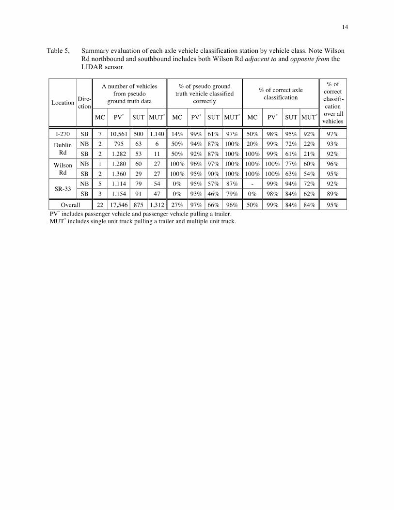
This pseudo ground truth analysis is repeated by individual station and Table 5 summarizes the performance. The first few columns report the number of vehicles seen in the pseudo ground truth for the given class, the next set of columns present the percentage of vehicles correctly classified in the given class, and the third set of columns present the percentage of axle classification by the given station that were correct in the given class. To help interpret these results, the final row of Table 5 summarizes Table 4. For example, the set of columns presenting the percentage of pseudo ground truth correctly classified in Table 5 reiterates the last column in Table 4. All stations report above 89% correct classification and most are above 92%. Table 4 shows the worst performance for motorcycles, with only 27% being correctly classified. As shown in Table 5, the temporary pneumatic tubes (Dublin Rd and Wilson Rd) were much better at detecting and classifying motorcycles than the permanent classification stations (I-270 and SR-33). Reviewing the data strictly from the two permanent classification stations, the pseudo ground truth include 15 motorcycles, of which only 1 (7%) was correctly classified by the classification stations. Meanwhile, 9 (60%) of the motorcycles were misclassified as longer vehicles and 5 (33%) passed completely undetected. Given the fact that these data come from only two classification stations and the number of motorcycles is small, further study is warranted.

Length-Based Classification Stations As noted in the introduction, we also used this methodology to evaluate the performance of length-based

classification. All of the permanent vehicle classification stations also provide length-based classification and we also tested the system at a single loop detector station on I-71 using Coifman and Kim (2009) for length-based classification. All vehicles below 28 ft are assigned to length class 1, all remaining vehicles below 47 ft are assigned to length class 2, and all vehicles above 47 ft are assigned length class 3; and these length classes are intended to roughly map to PV, SUT and MUT, respectively. So for our analysis we map LIDAR MC and PV to length class 1, LIDAR SUT to length class 2, and LIDAR MUT to length class 3. Tables 6 and 7 repeat the comparisons of the previous section, now applied to the length-based classification stations. The length-based performance and number of vehicle requiring manual validation are comparable to the axle-based classification performance.

DISCUSSION AND CONCLUSIONS

Vehicle classification data are critical to many transportation applications, but the quality of data collected depends on the operating agency to periodically calibrate, test, and validate the performance of classification sensors. All to often the performance evaluations necessary to ensure classification accuracy simply are not conducted because they are so labor intensive. When the studies are conducted, typically they are too coarse, allowing over-counting errors to cancel under-counting errors. Our group previously undertook a rigorous manual performance evaluation of several permanent classification stations selected at random and found that all of them exhibited chronic problems, e.g., at the time of evaluation, over 10% of the vehicles classified as multi-unit trucks from the existing stations were actually passenger vehicles. Most of these problems proved to be easy to fix once the error was detected. The results of this labor intensive effort showed the clear benefit of the performance evaluation; however, it is unrealistic to expect this level of labor to calibrate all stations, hence the motivation for the present work to automate most of the comparison process.

To address these challenges the present work develops a classification performance monitoring system to allow operating agencies to rapidly assess the health of their classification stations on a per vehicle basis. We eliminate most of the labor demands and instead, deploy a PNVCS to classify vehicles, concurrent with an existing classification station. To prevent classification errors from canceling one another in aggregate, we record per-vehicle record (pvr) data in the field from both systems. After the field collection the classification results are evaluated on a per-vehicle basis. This work requires several intermediate steps, developed herein, including synchronizing the independent clocks and matching observations of a given vehicle between the two classification systems. If the two systems agree for a given vehicle, it is automatically taken as a success by the classification station under the implicit assumptions: (i) That few vehicles will be misclassified the same way by the two independent systems. (ii) That the PNVCS has sufficient accuracy so that its data can be used as a benchmark for the existing classification station. For this application the PNVCS includes a time synchronized video camera to allow a human to assess the discrepancies. A human only looks at a given vehicle when the two systems disagree, and we developed tools to semi-automate the manual validation process, greatly increasing the efficiency and accuracy of the human user. The data sets in this study take only a few minutes for the user to validate an hour of pvr data. If personnel time were at a

8

premium one could even use a threshold to trigger manual review, e.g., if fewer than 5% of the vehicles were marked for manual review simply accept the existing classification station to be performing well enough. Still, the manual review should prove helpful in diagnosing the problems at those stations that fail this threshold test.

The primary objective of this study is to demonstrate the viability of our methodology to use a PNVCS to rapidly evaluate the performance of an existing vehicle classification station, regardless of the PNVCS technology used. This study uses a LIDAR based PNVCS but our basic approach is compatible with many other PNVCS, such as conventional pneumatic tubes or the newer TIRTL and AxleLight, provided the given PNVCS provides sufficient accuracy. Because of the LIDAR occlusions arising from the low mounting height, this analysis does not explicitly verify the classification station vehicle counts during the occlusions. However, if chronic errors are present that would degrade the occluded vehicle performance, they should still become evident via this work, e.g., if the classification station tends to miss motorcycles, we will not catch occluded motorcycles, but the error will still be evident over the many non-occluded motorcycles.

A secondary objective of this study is to demonstrate that our prototype LIDAR based PNVCS indeed offers the required accuracy for the performance evaluation. Conceptually the two systems should exhibit independent error patterns since the LIDAR approach relies on vehicle height while most conventional vehicle classification technologies rely on weight or magnetic length. Still, there may be some correlation between features (e.g., features that are functions of the vehicle length), and for those, the manual evaluation criteria could be broadened, e.g., "look at all vehicles that were within N ft of the length threshold." Such an extension proved unnecessary in the current work. A manual evaluation of 15,271 vehicles from which the LIDAR gave the same class as the existing classification station found that 99.8% were assigned the correct vehicle class. Furthermore, the LIDAR based PNVCS has previously demonstrated 99.5% classification accuracy (Lee and Coifman, 2012a).

The evaluation data sets come from several different classification stations and they include over 21,000 vehicles. We separately evaluated length-based classification stations and axle-based classification stations, each yielding similar results. The automated process does the bulk of the work. In each case about 8% of the vehicles required manual intervention. The user typically spent 3-5 sec per vehicle reviewed, translating into only a few minutes to process the exceptions from all lanes over one hour of data. The new method caught all of the errors that previously required a very labor intensive evaluation to find. This approach offers a cost effective solution to ensure that classification stations are providing accurate data. For permanent classification stations the additional labor is a fraction of the cost to deploy the station in the first place.

REFERENCES

Banks, J. (2008). Evaluation of Portable Automated Data Collection Technologies: Final Report. California PATH Research Report, UCB-ITSPRR-2008-15.

Caltrans (2007). VideoSync, http://www.dot.ca.gov/research/operations/videosync, accessed on December 2, 2011.

CEOS (2012). http://www.ceos.com.au/products/tirtl-content.htm, accessed November 15, 2012.

Coifman, B. and Cassidy, M. (2002). Vehicle Reidentification and Travel Time Measurement on Congested Freeways. Transportation Research: Part A, Vol 36, No 10, pp. 899-917.

Coifman, B. and Kim, S. (2009). Speed Estimation and Length Based Vehicle Classification from Freeway Single Loop Detectors. Transportation Research Part-C, Vol 17, No 4, pp 349-364.

Federal Highway Administration [FHWA] (2001). Traffic Monitoring Guide. USDOT, Office of Highway Policy Information, FHWA-PL-01-021.

French, J. and French, M. (2006). Traffic Data Collection Methodologies. Pennsylvania Department of Transportation, Contract 04-02 (C19).

Kim, S. and Coifman, B. (2013). Axle and Length Based Vehicle Classification Performance, Transportation Research Record: Journal of the Transportation Research Board, No. 2339, Transportation Research Board of the National Academies, Washington, DC, pp 1-12.

9

Kotzenmacher, J., Minge, E. and Hao, B. (2005). Evaluation of Portable Non-Intrusive Traffic Detection System. Minnesota Department of Transportation, MN-RC-2005-37.

Lee, H. and Coifman, B. (2012a). Side-Fire LIDAR Based Vehicle Classification. Transportation Research Record: 2308, Journal of the Transportation Research Board, Transportation Research Board of the National Academies, Washington, DC, pp 173-183.

Lee, H. and Coifman, B. (2012b). An Algorithm to Identify Chronic Splashover Errors at Freeway Loop Detectors, Transportation Research-Part C. Vol 24, pp 141-156.

Little, G., Johnson, M., and Zidek, P. (2001). Off-Road Axle Detection Sensor (ORADS) : Final Technical Report, Ohio Department of Transportation, FHWA/HWY-04/2001

Minge, E., (2010). Evaluation of Non-Intrusive Technologies for Traffic Detection. Minnesota Department of Transportation, Final Report #2010-36.

Minge, E., Petersen, S. and Kotzenmacher, J. (2011). Evaluation of Non-Intrusive Technologies for Traffic Detection - Phase 3. Transportation Research Record: Journal of the Transportation Research Board, No. 2256, Transportation Research Board of the National Academies, Washington, DC, pp. 95-103.

Peek Traffic, (2010), http://www.peektraffic.com/datasheets/axlelightdatasheet.pdf, accessed October 27, 2012.

Schwach, J., Morris, T., Michalopoulos, P. (2009). Rapidly Deployable Low-Cost Traffic Data and Video Collection Device, Center for Transportation Studies, University of Minnesota, CTS 09-21.

Spectra Research (2011). http://www.spectra-research.com/inner/electro.htm, accessed October 27, 2011.

Yu, X., Prevedouros, P., and Sulijoadikusumo, G. (2010). Evaluation of Autoscope, SmartSensor HD, and Infra-Red Traffic Logger for Vehicle Classification. Transportation Research Record: Journal of the Transportation Research Board, No. 2160, Transportation Research Board of the National Academies, Washington, DC, pp. 77-86.

Zwahlen, H. T., Russ, A., Oner, E., and Parthasarathy, M. (2005). Evaluation of Microwave Radar Trailers for Non-intrusive Traffic Measurements. Transportation Research Record: Journal of the Transportation Research Board, No. 1917, Transportation Research Board of the National Academies, Washington, DC, pp. 127-140.

10

Table 1, Summary of the automated comparison of vehicle classification between LIDAR and axle data at seven directional classification stations

LIDAR sensor

direction relative to

vehicle travel

direction

Loca- tion

(direc- tion)

Date

Dura- tion (hh: min)

Lane num- ber

from LIDAR

Number of vehicles seen

in;

From the algorithm of vehicle matching

Number of

vehicles passing

the location

(f)

Number of

partially occluded vehicles

(g)

Comparison of vehicle

classification

% vehicles not detected by; Number of

vehicles manually confirmed

(l)

Number of

vehicles seen in

both LIDAR

and Axle (c)

Number of vehicles only

seen in;

LIDAR (a)

Axle (b)

LIDAR (d)

Axle (e)

Number of

compared vehicles

(h)

Dis- agree- ment

(i)

LIDAR (j)

Axle (k)

Adjacent

I-270 (SB) 11/02/2010 5:00

1 5,415 5,452 5,389 26 63 5,478 n/a 5,389 188 (3.5%) 1.2% 0.5% 277

(5.1%)

2 5,335 5,488 5,303 32 185 5,520 641 4,662 145 (3.1%) 3.4% 0.6% 362

(6.6%)

3 2,647 2,789 2,615 32 174 2,821 713 1,902 24 (1.3%) 6.2% 1.1% 230

(8.2%) Dublin (SB) 10/28/2010 2:50 1 1,344 1,317 1,313 31 4 1,348 n/a 1,313 80

(6.1%) 0.3% 2.3% 115 (8.5%)

Wilson (NB) 10/28/2010 1:40 1 666 664 658 8 6 672 n/a 658 24

(3.6%) 0.9% 1.2% 38 (5.7%)

Wilson (SB) 10/28/2010 1:40 1 711 712 701 10 11 722 n/a 701 21

(3.0%) 1.5% 1.4% 42 (5.8%)

SR-33 (NB) 08/03/2011 1:10

1 732 693 684 48 9 741 n/a 684 32 (4.7%) 1.2% 6.5% 89

(12.0%)

2 569 562 547 22 15 584 65 482 6 (1.2%) 2.6% 3.8% 43

(7.4%)

Subtotal of adjacent 12:20 - 17,419 17,677 17,210 209 467 17,886 1,419 15,791 520 (3.3%) 2.6% 1.2% 1,196

(6.7%)

Opposite

Dublin (NB) 10/28/2010 2:50 2 940 943 933 7 10 950 75 858 52

(6.1%) 1.1% 0.7% 69 (7.3%)

Wilson (NB) 10/28/2010 1:40 2 749 752 742 7 10 759 58 684 18

(2.6%) 1.3% 0.9% 35 (4.6%)

Wilson (SB) 10/28/2010 1:40 2 741 735 723 18 12 753 47 676 24

(3.6%) 1.6% 2.4% 54 (7.2%)

SR-33 (SB) 08/03/2011 1:10

3 592 587 548 44 39 631 53 495 9 (1.8%) 6.2% 7.0% 92

(14.6%)

4 888 884 838 50 46 934 148 690 54 (7.8%) 4.9% 5.4% 150

(16.1%)

Subtotal of opposite 7:20 - 3,910 3,901 3,784 126 117 4,027 381 3,403 157 (4.6%) 2.9% 3.1% 400

(9.9%)

Overall 19:40 - 21,329 21,578 20,994 335 584 21,913 1,800 19,194 677 (3.5%) 2.7% 1.5% 1,596

(7.3%) n/a: occlusions are infeasible in this lane because it is adjacent to the LIDAR sensor (a) = (c + d) (b) = (c + e) (f) = (a + e) = (b + d) (h) = (c) – (g) (j) = (e) / (f) (k) = (d) / (f) (l) = (d + e + i), where the percentage is relative to (f)

11

Table 2, Manual verification of the vehicles with conflicting classifications or only seen by one system using the semi-automated tool

LIDAR sensor

direction relative to

vehicle travel

direction

Loca- tion

(direc- tion)

Lane num- ber

from LIDAR

Number of vehicles

not detected

by LIDAR (e)

Reason

Number of vehicles

not detected by Axle

(d)

Reason Number

of vehicles

in disagree-

ment (i)

Verification of disagreement

% axle miss-

classified (r)

% total axle error (s)

Totally occluded vehicle

LIDAR missed vehicle

Axle non-

vehicle actuation

(m)

Axle missed vehicle

(n)

LIDAR non-

vehicle actuation

LIDAR correct,

Axle incorrect

(p)

LIDAR incorrect,

Axle correct

LIDAR incorrect

Axle incorrect

(q)

Adjacent

I-270 (SB)

1 63 n/a 63 0 26 26 0 188 148 36 4 2.8% 3.2%

2 185 116 69 0 32 32 0 145 113 30 2 2.5% 2.6%

3 174 141 33 0 32 32 0 24 20 4 0 1.1% 1.7% Dublin (SB) 1 4 n/a 4 0 31 31 0 80 76 4 0 5.8% 7.9%

Wilson (NB) 1 6 n/a 6 0 8 8 0 24 22 2 0 3.3% 4.5%

Wilson (SB) 1 11 n/a 11 0 10 10 0 21 18 3 0 2.6% 3.9%

SR-33 (NB)

1 9 n/a 9 0 48 48 0 32 26 4 2 4.1% 10.3%

2 15 8 7 0 22 22 0 6 5 1 0 1.0% 4.5%

Subtotal of adjacent 467 265 202 0 209 209 0 520 428 84 8 2.8% 3.6%

Opposite

Dublin (NB) 2 10 5 1 4 7 7 0 52 48 3 1 5.7% 6.3%

Wilson (NB) 2 10 5 5 0 7 7 0 18 15 3 0 2.2% 2.9%

Wilson (SB) 2 12 10 2 0 18 18 0 24 22 2 0 3.3% 5.3%

SR-33 (SB)

3 39 27 12 0 44 44 0 9 6 3 0 1.2% 7.9%

4 46 41 4 1 50 50 0 54 42 11 1 6.2% 10.1%

Subtotal of opposite 117 88 24 5 126 126 0 157 133 22 2 4.0% 6.6%

Overall 584 353 226 5 335 335 0 677 561 106 10 3.0% 4.1% n/a: occlusions are infeasible in this lane because it is adjacent to the LIDAR sensor (r) = (p+q) / (h) (s) = (p+q+m+n)/(f-m) Note (f) and (h) are shown in Table 1.

12

Table 3, Comparison of LIDAR vehicle classification and axle vehicle classification across seven directional locations

Overall

Axle vehicle classification Number of LIDAR vehicles

not detected by axle sensor

Total number of

LIDAR vehicles

Motor- cycle

Passenger vehicle*

Single unit

truck

Multiple unit

truck*

LIDAR vehicle

classification

Motorcycle 6 12 1 0 12 31 Passenger vehicle* 2 16,751 127 159 283 17,322 Single unit truck 1 212 530 96 28 867

Multiple unit truck* 1 47 19 1,230 12 1,309 Number of axle vehicles

not detected by LIDAR sensor 3 555 10 16 - 584

Total number of axle vehicles above 13 17,577 687 1,501 335 20,113

Number of partially occluded vehicles excluded

in the comparison matrix 2 1,571 56 171 - 1,800

Passenger vehicle* includes passenger vehicle and passenger vehicle pulling a trailer. Multiple unit truck* includes single unit truck pulling a trailer and multiple unit truck.

13

Table 4, Comparison of pseudo ground truth data and axle vehicle classification across seven directional locations

Overall

Axle vehicle classification Number of LIDAR vehicles not detected by

axle sensor

Row total

%

correct Motor- cycle

Passenger vehicle*

Single unit

truck

Multiple unit

truck*

Pseudo ground

truth data

Motorcycle 6 2 6 3 5 22 27%

Passenger vehicle* 2 17,001 94 160 289 17,546 97%

Single unit truck 1 196 574 79 25 875 66%

Multiple unit truck* 1 30 9 1,256 16 1,312 96%

Non-vehicle actuation in axle data 2 3 0 0 - 5 -

Column total above 12 17,232 683 1,498 335 19,760 - % correct 50% 99% 84% 84% - - 95%

Totally occluded vehicle 1 345 4 3 - 353 - Passenger vehicle* includes passenger vehicle and passenger vehicle pulling a trailer. Multiple unit truck* includes single unit truck pulling a trailer and multiple unit truck.

14

Table 5, Summary evaluation of each axle vehicle classification station by vehicle class. Note Wilson Rd northbound and southbound includes both Wilson Rd adjacent to and opposite from the LIDAR sensor

Location Dire- ction

A number of vehicles from pseudo

ground truth data

% of pseudo ground truth vehicle classified

correctly

% of correct axle classification

% of correct

classifi- cation

over all vehicles MC PV* SUT MUT* MC PV* SUT MUT* MC PV* SUT MUT*

I-270 SB 7 10,561 500 1,140 14% 99% 61% 97% 50% 98% 95% 92% 97%

Dublin Rd

NB 2 795 63 6 50% 94% 87% 100% 20% 99% 72% 22% 93% SB 2 1,282 53 11 50% 92% 87% 100% 100% 99% 61% 21% 92%

Wilson Rd

NB 1 1,280 60 27 100% 96% 97% 100% 100% 100% 77% 60% 96% SB 2 1,360 29 27 100% 95% 90% 100% 100% 100% 63% 54% 95%

SR-33 NB 5 1,114 79 54 0% 95% 57% 87% - 99% 94% 72% 92% SB 3 1,154 91 47 0% 93% 46% 79% 0% 98% 84% 62% 89%

Overall 22 17,546 875 1,312 27% 97% 66% 96% 50% 99% 84% 84% 95% PV* includes passenger vehicle and passenger vehicle pulling a trailer. MUT* includes single unit truck pulling a trailer and multiple unit truck.

15

Table 6, Comparison of pseudo ground truth data and length-based vehicle classification across four directional locations

Overall Length class from

loop detector Number of

LIDAR vehicles not detected

by loop detector

Row total

% correct

Class 1 Class 2 Class 3

Pseudo ground truth data

Passenger vehicle* 15,623 256 66 271 16,216 96%

Single unit truck 125 590 8 26 749 79%

Multiple unit truck* 21 23 1,286 16 1,346 96%

Non-vehicle actuation in loop detector data 1 0 0 - 1 -

Column total above 15,770 869 1,360 313 18,312 -

% correct 99% 68% 95% - - 96%

Totally occluded vehicles 498 7 5 - 510 -

Passenger vehicle* includes passenger vehicle and passenger vehicle pulling a trailer. Multiple unit truck* includes single unit truck pulling a trailer and multiple unit truck.

16

Table 7, Summary evaluation of each length-based vehicle classification station by vehicle class

Location (traffic

condition)

Dire- ction

A number of vehicles from pseudo

ground truth data

% of pseudo ground truth vehicle

classified correctly

% of correct loop classification

% of correct

classification over all vehicles

Class 1 Class 2 Class 3 Class 1 Class 2 Class 3 Class 1 Class 2 Class 3

I-71 (free flow) SB 1,428 32 51 96% 50% 94% 99% 42% 84% 95%

I-71 (Congestion) SB 1,967 38 40 97% 61% 98% 99% 47% 95% 97%

I-270 (free flow) SB 10,546 509 1,153 97% 92% 97% 99% 70% 95% 97%

SR-33 (free flow)

NB 1,117 81 54 94% 69% 81% 98% 79% 96% 92%

SB 1,158 89 48 92% 31% 73% 95% 60% 92% 87%

17

Figure 1, Flowchart of the evaluation of an existing vehicle classification station using LIDAR PNVCS

vehicle classification.

Time synchronization

Vehicle matching (Search for corresponding

vehicles from two data sets)

Comparison of vehicleclassification from

non-occluded vehicles

Agreement of vehicle classification

Disagreement of vehicle classification

Manual verification of vehicles using

semi-automated tool

Vehicles seenin the both data sets(matched vehicle)

Vehicles only seenin one data set

(unmatched vehicle)

Count vehicles that were partially occluded in the

LIDAR, but do not compare

Automatically consideredas success

Traffic stream

Video recording(time synchronized

with LIDAR)

Final result

Classification stationpvr data

Classifier under evaluation

LIDAR pvrclassification data

LIDAR based vehicleclassification algorithm

18

Figure 2, A hypothetical example of a vehicle passing by the two side-fire LIDAR sensors: (a) in time-

space plane and (b) a top-down schematic of the scene at an instant. (c) A photograph of the LIDAR equipped van showing the sensors used in this study.

19

Figure 3, RVMK versus the resulting offset time as a function of K from SR-33 northbound, (a) Lane 1,

the peak shows the final offset time is -436.6 sec, and (b) Lane 2, the peak shows the final offset time is -436.5 second.

(a)

(b)

20

Figure 4, (a) A feasible vehicle matrix, summarizing the outcome from the difference of arrival times

between the LIDAR and classification station data in lane 1 at SR-33 northbound. (b-d) extreme hypothetical example: (b) hypothetical feasible vehicle matrix in which many rows and columns have multiple matches, (c) isolating the distinct groups of vehicles, the groups are numbered for reference, (d) selecting the longest sequence from the given group. Note that the two sequences in group 2 are equal length, so the algorithm would then compare the classification results from the two systems and select the sequence with the strongest similarity between the two systems.

“○” = possible match = a group associated with multiple matches

= rejected matches

3

X= pending matches

LID

AR

veh

icle

#

Classification station vehicle # Classification station vehicle #

LID

AR

veh

icle

#

1

2

LID

AR

veh

icle

#Classification station vehicle #

X

XX

X

1

23

(b) (c) (d)

(a)

21

Figure 5, A snapshot of the semi-automated GUI verification tool processing a conflicting

classification for a vehicle in lane 1 at SR-33 northbound. The GUI window consists of four interfaces: (a) plot of transition pulses, the plot shows for each lane the classification station data (top curve) and LIDAR data (bottom curve) and the current instant is shown with a vertical dashed line, (b) the current video frame, (c) the LIDAR returns from the vehicle in question, and (d) a panel for controlling the review and entering ground truth data. So in this case the GUI is at the second visible pulse in lane 1 (counted from the left hand side) and is ready for the user to assess the data using the buttons on the right of part (d).

(b) (c)

(d)

Lane number

Time (hr)

(a)

ContactsFormoreinformation:

BenjaminCoifman,PhDTheOhioStateUniversityDepartmentofCivil,Environmental,andGeodeticEngineeringHitchcockHall4702070NeilAve,Columbus,OH43210(614)292-4282Coifman.1@OSU.eduhttps://ceg.osu.edu/~coifman

NEXTRANSCenterPurdueUniversity-DiscoveryPark3000KentAve.WestLafayette,IN47906nextrans@purdue.edu(765)496-9724www.purdue.edu/dp/nextrans