li z., zhou m. deadlock resolution in automated manufacturing systems - a novel petri net approach
TRANSCRIPT

8/4/2019 Li Z., Zhou M. Deadlock Resolution in Automated Manufacturing Systems - A Novel Petri Net Approach
http://slidepdf.com/reader/full/li-z-zhou-m-deadlock-resolution-in-automated-manufacturing-systems-a-novel 1/249
Advances in Industrial Control

8/4/2019 Li Z., Zhou M. Deadlock Resolution in Automated Manufacturing Systems - A Novel Petri Net Approach
http://slidepdf.com/reader/full/li-z-zhou-m-deadlock-resolution-in-automated-manufacturing-systems-a-novel 2/249

8/4/2019 Li Z., Zhou M. Deadlock Resolution in Automated Manufacturing Systems - A Novel Petri Net Approach
http://slidepdf.com/reader/full/li-z-zhou-m-deadlock-resolution-in-automated-manufacturing-systems-a-novel 3/249
ZhiWu Li • MengChu Zhou
Deadlock Resolution
in Automated Manufacturing
SystemsA Novel Petri Net Approach
123

8/4/2019 Li Z., Zhou M. Deadlock Resolution in Automated Manufacturing Systems - A Novel Petri Net Approach
http://slidepdf.com/reader/full/li-z-zhou-m-deadlock-resolution-in-automated-manufacturing-systems-a-novel 4/249
ZhiWu Li, PhD
School of Electro-Mechanical
Engineering
Xidian University
2 South TaiBai Road710071 Xi’an
China
MengChu Zhou, PhD
Department of Electrical and Computer
Engineering
New Jersey Institute of Technology
323 MLK Blvd.Newark
NJ 07102-1982
USA
ISBN 978-1-84882-243-6 e-ISBN 978-1-84882-244-3
DOI 10.1007/978-1-84882-244-3
Advances in Industrial Control series ISSN 1430-9491
A catalogue record for this book is available from the British Library
Library of Congress Control Number: 2009921446
© 2009 Springer-Verlag London Limited
Apart from any fair dealing for the purposes of research or private study, or criticism or review, as
permitted under the Copyright, Designs and Patents Act 1988, this publication may only be
reproduced, stored or transmitted, in any form or by any means, with the prior permission in writing of the publishers, or in the case of reprographic reproduction in accordance with the terms of licences
issued by the Copyright Licensing Agency. Enquiries concerning reproduction outside those terms
should be sent to the publishers.
The use of registered names, trademarks, etc. in this publication does not imply, even in the absence of
a specific statement, that such names are exempt from the relevant laws and regulations and therefore
free for general use.
The publisher makes no representation, express or implied, with regard to the accuracy of the
information contained in this book and cannot accept any legal responsibility or liability for any errors
or omissions that may be made.
Cover design: eStudio Calamar S.L., Girona, Spain
Printed on acid-free paper
9 8 7 6 5 4 3 2 1
springer.com

8/4/2019 Li Z., Zhou M. Deadlock Resolution in Automated Manufacturing Systems - A Novel Petri Net Approach
http://slidepdf.com/reader/full/li-z-zhou-m-deadlock-resolution-in-automated-manufacturing-systems-a-novel 5/249
Advances in Industrial Control
Series Editors
Professor Michael J. Grimble, Professor of Industrial Systems and Director
Professor Michael A. Johnson, Professor (Emeritus) of Control Systems and Deputy Director
Industrial Control Centre
Department of Electronic and Electrical Engineering
University of Strathclyde
Graham Hills Building
50 George Street
Glasgow G1 1QE
United Kingdom
Series Advisory Board
Professor E.F. Camacho
Escuela Superior de Ingenieros
Universidad de Sevilla
Camino de los Descubrimientos s/n
41092 Sevilla
Spain
Professor S. EngellLehrstuhl für Anlagensteuerungstechnik
Fachbereich Chemietechnik
Universität Dortmund
44221 Dortmund
Germany
Professor G. Goodwin
Department of Electrical and Computer Engineering
The University of Newcastle
Callaghan
NSW 2308
Australia
Professor T.J. Harris
Department of Chemical Engineering
Queen’s University
Kingston, Ontario
K7L 3N6
Canada
Professor T.H. Lee
Department of Electrical and Computer Engineering
National University of Singapore
4 Engineering Drive 3
Singapore 117576

8/4/2019 Li Z., Zhou M. Deadlock Resolution in Automated Manufacturing Systems - A Novel Petri Net Approach
http://slidepdf.com/reader/full/li-z-zhou-m-deadlock-resolution-in-automated-manufacturing-systems-a-novel 6/249
Professor (Emeritus) O.P. Malik
Department of Electrical and Computer Engineering
University of Calgary
2500, University Drive, NW
Calgary, AlbertaT2N 1N4
Canada
Professor K.-F. Man
Electronic Engineering Department
City University of Hong Kong
Tat Chee Avenue
Kowloon
Hong Kong
Professor G. OlssonDepartment of Industrial Electrical Engineering and Automation
Lund Institute of Technology
Box 118
S-221 00 Lund
Sweden
Professor A. Ray
Department of Mechanical Engineering
Pennsylvania State University
0329 Reber BuildingUniversity Park
PA 16802
USA
Professor D.E. Seborg
Chemical Engineering
3335 Engineering II
University of California Santa Barbara
Santa Barbara
CA 93106
USA
Doctor K.K. Tan
Department of Electrical and Computer Engineering
National University of Singapore
4 Engineering Drive 3
Singapore 117576
Professor I. Yamamoto
Department of Mechanical Systems and Environmental Engineering
The University of Kitakyushu
Faculty of Environmental Engineering
1-1, Hibikino,Wakamatsu-ku, Kitakyushu, Fukuoka, 808-0135
Japan
8/4/2019 Li Z., Zhou M. Deadlock Resolution in Automated Manufacturing Systems - A Novel Petri Net Approach
http://slidepdf.com/reader/full/li-z-zhou-m-deadlock-resolution-in-automated-manufacturing-systems-a-novel 7/249
in memory of my mother,
YuQing Zhang
(ZWL)
for my family, Fang Chen, Albert and Benjamin
(MCZ)

8/4/2019 Li Z., Zhou M. Deadlock Resolution in Automated Manufacturing Systems - A Novel Petri Net Approach
http://slidepdf.com/reader/full/li-z-zhou-m-deadlock-resolution-in-automated-manufacturing-systems-a-novel 8/249
ix
Series Editors’ Foreword
The series Advances in Industrial Control aims to report and encourage
technology transfer in control engineering. The rapid development of control
technology has an impact on all areas of the control discipline. New theory, new
controllers, actuators, sensors, new industrial processes, computer methods, new
applications, new philosophies…, new challenges. Much of this developmentwork resides in industrial reports, feasibility study papers and the reports of
advanced collaborative projects. The series offers an opportunity for researchersto present an extended exposition of such new work in all aspects of industrial
control for wider and rapid dissemination.Much of the technological infrastructure of modern society is comprised of
large networked dynamical systems. These systems include transportation (road,
rail, air), energy networks (gas, electricity, oil), resource networks (water supply,
wastewater disposal) and information networks (the Internet, information systems
for transportation). Integrated with these are the primary industries that take raw
material inputs and produce refined outputs like steel, paper, petroleum products,
power and so on. The outputs of the primary industries supply secondary
industries that manufacture both complex and simple products ranging from
aircraft and automobiles, to computers, consumer white goods, food and
pharmaceutical products. These are all process and manufacturing areas wherecontrol engineering plays an essential role.
The control communities approach to the modelling, analysis and design
problems of industrial processes and networks has been threefold. Firstly,
methods for continuous-time systems have been developed progressively since the
1940s and are now very well established but even these methods are still evolving
especially in the nonlinear systems area. Secondly, there has been the rise of
methods for discrete-event dynamical systems; this has often used ideas first
devised by the computer science community. Finally, since about the 1980s, the
idea of a hybrid system approach has gained credence and this paradigm is stillunder development.
In the Advances in Industrial Control monograph series and the Advanced Textbooks in Control and Signal Processing series, we have sought to feature

8/4/2019 Li Z., Zhou M. Deadlock Resolution in Automated Manufacturing Systems - A Novel Petri Net Approach
http://slidepdf.com/reader/full/li-z-zhou-m-deadlock-resolution-in-automated-manufacturing-systems-a-novel 9/249
x Series Editors’ Foreword
titles that cover all aspects of this growth of the control field. For example, the
modelling and analysis of discrete-event processes involves the challenging issues
of resource allocation, logical decision-making, timed-event activity, and
constraint handling. Within the Advanced Textbooks in Control and Signal
Processing series, many of the latest developments in this field have beencaptured in Modeling and Control of Discrete-event Dynamical Systems by
Branislav Hrúz end MengChu Zhou (ISBN 978-1-84628-872-2, 2007). This book
is particularly relevant here because it contains an excellent introduction to the
modelling and analysis tools of Petri nets, which have been used by various
authors to solve some of the discrete, logical and continuous modelling, analysis
and design problems of advanced industrial processes.
One entry to the Advances in Industrial Control series has been Modelling and Analysis of Hybrid Supervisory Systems by Emilia Villani, Paulo E. Miyagi, and
Robert Valette (ISBN 978-1-84628-650-6, 2007). This reported a new technique
that built on the capabilities of Petri nets and captured the realistic behaviour of large and small complex mixed dynamical discrete and continuous industrial
systems. The method was demonstrated on three complex industrial examples, a
heating, ventilation, and air conditioning system, an aircraft landing system and a
cane-sugar production plant.
Continuing with the emphasis on solving real industrial control and
supervisory control problems, this entry to Advances in Industrial Control by
ZhiWu Li and MengChu Zhou tackles the deadlock problem using the formalism
of Petri nets. It is an exhaustive text for this area of research and proposes new
solutions for a long-standing problem. The reader who already has somefamiliarity with Petri nets and the associated analysis techniques will benefit
directly; however, the inclusion of an introductory chapter on Petri nets makesthis book self-contained. It can be usefully supplemented by reading the Petri net
chapters in the above-mentioned Hrúz and Zhou textbook. The penultimate
chapter of Deadlock Resolution in Automated Manufacturing Systems alsocompares a range of deadlock prevention policies and many readers interested in
automated manufacturing will find this a useful source of ideas and further reading. The Editors of the Advances in Industrial Control series welcome this
book as a valuable addition to the growing literature on these important, complex
and large-scale industrial problems.
Industrial Control Centre M.J. GrimbleGlasgow M.A. Johnson
Scotland, UK
2008

8/4/2019 Li Z., Zhou M. Deadlock Resolution in Automated Manufacturing Systems - A Novel Petri Net Approach
http://slidepdf.com/reader/full/li-z-zhou-m-deadlock-resolution-in-automated-manufacturing-systems-a-novel 10/249
Preface
The rapid evolution of computing, communication, control, and sensor technologies
has brought about the proliferation of new man-made dynamic systems, mostly tech-
nological and often highly complex. Examples around us are air traffic control sys-
tems; automated manufacturing systems; computer and communication networks;
embedded and networked systems; and software systems. The activity in these sys-
tems is governed by operational rules designed by humans and their dynamics is
often driven by asynchronous occurrences of discrete events. This class of dynamic
systems is therefore called discrete-event (dynamic) systems.
Based on finite-state automata and formal languages, the seminal work by Ra-
madge and Wonham in the early 1980s aims at providing a comprehensive and
structural treatment of the modeling and control of discrete-event systems (DESs).
The results in this area are gradually shaped and lead to supervisory control theory
(SCT). SCT considers a DES as a generator of a formal language. Its behavior can
be controlled by a supervisor that prevents event occurrences in order to satisfy a
given specification.
Due to its generality, SCT is a paradigm that bridges the two worlds of control
theory and computer science. In the latter, there exists a well-established Petri net
community. As a natural and alternative modeling formalism, Petri nets are widely
used for DES modeling and control. Their structural properties have been success-
fully exploited for the design of supervisors for supervisory control problems. Sig-
nificant progress in this direction was made over the last two decades. The results
obtained so far deal mainly with the safety of a plant, i.e., avoidance of dangerous
or forbidden conditions given in a control specification. Liveness in Petri nets is an
important behavioral property that leads to the safety of the supervised plant. It im-
plies the freedom of deadlock–a highly undesired situation that an automated system
must completely avoid. This property is equivalent to the non-blockingness in SCT.
SCT is independent of the specific representation. That is to say, it is independent
of a specific implementation technology.A variety of theoretical results and computational algorithms have been devel-
oped in the literature to assess the liveness of certain classes of Petri nets. Most of
these results are based on the fact that the liveness of a Petri net is closely related
xi

8/4/2019 Li Z., Zhou M. Deadlock Resolution in Automated Manufacturing Systems - A Novel Petri Net Approach
http://slidepdf.com/reader/full/li-z-zhou-m-deadlock-resolution-in-automated-manufacturing-systems-a-novel 11/249
xii Preface
to the satisfiability of certain predicates on siphons. As a set of place elements, a
siphon is a structural object in Petri nets. This relation between liveness and siphons
becomes strong and apparent when we investigate the practical DES including a va-
riety of resource allocation systems in a contemporary technological domain. Con-
sequently, the siphon-based characterization of liveness and liveness-enforcing su-pervision for DESs modeled with Petri nets is usually considered to be one of the
most interesting developments in the last decade from both theoretical and practical
points of view.
However, the power of siphon-based liveness-enforcing approaches is degraded
and deteriorated as the number of siphons grows quickly beyond practical limits and
in the worst case grows exponentially fast with respect to the Petri net size. They
suffer from the computational complexity problem since it is known that in general
the complete siphon enumeration in a Petri net is NP-complete. Furthermore, they
usually lead to a much more structurally complex liveness-enforcing Petri net super-
visor than the plant net model that is originally built. This book tries to show how
an elementary siphon-based methodology tackles these problems.
The book is intended for researchers, graduate students, and engineers who are
interested in the control problems arising from manufacturing, transportation, work-
flow systems, communication, computer networks, complex software, and chemical
industry. It is also appropriate for the students in automatic control, computer sci-
ence, and applied mathematics and can be used as a supplementary textbook in the
courses on Petri net theory and applications as well as the supervisory control of
DESs.
Nevertheless, we try to maintain as a goal the presentation of a detailed discus-
sion of the fundamental aspects of the related theory used throughout this book and
hope to give readers a sufficiently solid foundation for their own advanced work
and further study of the literature on this subject, it is highly desired that readers
are familiar with the basics of linear algebra, set theory, and (integer) linear pro-
gramming. In this sense, this book is self-contained. However, it is not intended
to be an introductory textbook on Petri net theory. Being already familiar with net
theory is hardly necessary to open this book but surely helpful if readers know its
preliminaries.
Following the introduction in Chap. 1, the basics of Petri nets are presented inChap. 2, which is used throughout this book. Explanatory examples are given to
illustrate the concepts so that readers can understand the book without the prior
knowledge of general Petri net theory. The concept of elementary and dependent
siphons in a net is proposed in Chap. 3. As a natural extension to the concept of ele-
mentary siphons, Chap. 4 presents a novel monitor implementation to enforce gen-
eralized mutual exclusion constraints (GMECs). Chap. 5 presents a number of dead-
lock prevention policies that are developed on the basis of elementary siphons. The
role of elementary siphons is fully shown in Chap. 6 by investigating the existence
of a maximally permissive (optimal) liveness-enforcing monitor-based Petri net su-pervisor for a flexible manufacturing system. A survey and comparison of a variety
of deadlock prevention policies in the literature are presented in Chap. 7. The com-
parison is conducted from the following points of view: computational complexity,

8/4/2019 Li Z., Zhou M. Deadlock Resolution in Automated Manufacturing Systems - A Novel Petri Net Approach
http://slidepdf.com/reader/full/li-z-zhou-m-deadlock-resolution-in-automated-manufacturing-systems-a-novel 12/249
Preface xiii
structural complexity, and behavior permissiveness. The last chapter concludes this
book by summarizing the results in the literature and presenting some interesting
and open problems as well as some guidelines to tackle them.
Attached to the end of every chapter is a reference bibliography, and a glossary
and a complete index in the final part, which should facilitate readers in using thisbook.
Readers of this book can learn the basics of Petri nets, siphon-based characteriza-
tion of liveness, the theory of elementary siphons, and deadlock resolution methods
and strategies for automated manufacturing systems. They can also learn a number
of deadlock prevention policies developed on the basis of elementary siphons. They
can finally master the concept of elementary siphons and related methods in design-
ing structurally simple liveness-enforcing monitor-based Petri net supervisors.
Xidian University, China ZhiWu LiNew Jersey Institute of Technology, USA MengChu Zhou
August 2008

8/4/2019 Li Z., Zhou M. Deadlock Resolution in Automated Manufacturing Systems - A Novel Petri Net Approach
http://slidepdf.com/reader/full/li-z-zhou-m-deadlock-resolution-in-automated-manufacturing-systems-a-novel 13/249
Acknowledgments
We are very grateful to Professor W. M. Wonham, Department of Electrical and
Computer Engineering, University of Toronto, Professor M. D. Jeng, Department
of Electrical Engineering, National Taiwan Ocean University, Professor X. L. Xie,
INRIA, France, Professor Y. S. Huang, Department of Aeronautical Engineering,
Chung Cheng Institute of Technology, National Defense University (Taiwan), Pro-
fessor M. Uzam, Nigde Universitesi, Professor N. Q. Wu, Department of Mecha-
tronics Engineering, Guangdong University of Technology, Professor Y. Chao, De-
partment of Management and Information Science, National Cheng Chi University,
L. Feng, KTH-Royal Institute of Technology, and F. Lewis, The University of Texas
at Arlington, for their valuable comments and suggestions to our research.
We would like to express our sincere gratitude and appreciation to Professor M.
Shpitalni for hosting the first author of this book as a visiting professor from Febru-
ary 2007 to February 2008 in the Laboratory for CAD & Life-cycle Engineering,
Department of Mechanical Engineering, Technion-Israel Institute of Technology.
The first author would like to wholeheartedly thank his wife, TongLing Feng,
and his son, BuZi Li, for their superhuman patience and sacrifice, and consistent en-
couragement. They have graciously endured many long nights and lonely weekends
while he was immersed in his research.
A tribute is due to the unceasing efforts of the numerous investigators in this
area, whose scientific contributions are directly responsible for the creation of this
book. Among them are K. Barkaoui, Y. Chao, J. Ezpeleta, M. P. Fanti, A. Giua,
Y. S. Huang, M. V. Iordache, M. D. Jeng, K. Lautenbach, F. Lewis, J. Park, S. A.
Reveliotis, E. Roszkowska, F. G. Tricas, M. Uzam, N. Q. Wu, X. L. Xie, and K. Y.
Xing.
Finally, the authors would like to thank the following students: A. R. Wang, H.
S. Hu, M. Zhao, N. Wei, M. M. Yan, D. Liu, C. F. Zhong, M. Qin, G. Y. Liu, and Y.
F. Hou. We appreciate their hard work in this area, particularly during the difficult
times that we had in past years.This work was in part supported by the National Nature Science Foundation of
China under Grant No. 60228004, 60474018, and 60773001, the Scientific Research
Foundation for the Returned Overseas Chinese Scholars, the Ministry of Education,
xv

8/4/2019 Li Z., Zhou M. Deadlock Resolution in Automated Manufacturing Systems - A Novel Petri Net Approach
http://slidepdf.com/reader/full/li-z-zhou-m-deadlock-resolution-in-automated-manufacturing-systems-a-novel 14/249
xvi Acknowledgments
P. R. China, under Grant No. 2004-527, the Laboratory Foundation for the Returned
Overseas Chinese Scholars, the Ministry of Education, P. R. China, under Grant
No. 030401, Chang Jiang Scholars Program, the Ministry of Education, P. R. China,
the National Research Foundation for the Doctoral Program of Higher Education,
the Ministry of Education, P. R. China, under Grant No. 20070701013, Technion-Xidian Academic Exchange Program, “863” High-tech Research and Development
Program of China, under Grant No. 2008AA04Z109, and the New Jersey Commis-
sion on Science and Technology.

8/4/2019 Li Z., Zhou M. Deadlock Resolution in Automated Manufacturing Systems - A Novel Petri Net Approach
http://slidepdf.com/reader/full/li-z-zhou-m-deadlock-resolution-in-automated-manufacturing-systems-a-novel 15/249
Contents
Abbreviations . . . . . . . . . . . . . . . . . . . . . . . . . . . . . . . . . . . . . . . . . . . . . . . . . . xxi
1 Introduction . . . . . . . . . . . . . . . . . . . . . . . . . . . . . . . . . . . . . . . . . . . . . . . . . . . 1
1.1 Background . . . . . . . . . . . . . . . . . . . . . . . . . . . . . . . . . . . . . . . . . . . . . . . 1
1.2 Literature Review . . . . . . . . . . . . . . . . . . . . . . . . . . . . . . . . . . . . . . . . . . 3
1.3 Outline of the Book . . . . . . . . . . . . . . . . . . . . . . . . . . . . . . . . . . . . . . . . . 9
1.4 Bibliographical Remarks . . . . . . . . . . . . . . . . . . . . . . . . . . . . . . . . . . . . 10
Problems . . . . . . . . . . . . . . . . . . . . . . . . . . . . . . . . . . . . . . . . . . . . . . . . . . . . . . 10
References . . . . . . . . . . . . . . . . . . . . . . . . . . . . . . . . . . . . . . . . . . . . . . . . . . . . . 10
2 Petri Nets . . . . . . . . . . . . . . . . . . . . . . . . . . . . . . . . . . . . . . . . . . . . . . . . . . . . . 17
2.1 Introduction . . . . . . . . . . . . . . . . . . . . . . . . . . . . . . . . . . . . . . . . . . . . . . . 17
2.2 Formal Definitions . . . . . . . . . . . . . . . . . . . . . . . . . . . . . . . . . . . . . . . . . 17
2.3 Structural Invariants . . . . . . . . . . . . . . . . . . . . . . . . . . . . . . . . . . . . . . . . 25
2.4 Siphons and Traps . . . . . . . . . . . . . . . . . . . . . . . . . . . . . . . . . . . . . . . . . . 27
2.5 Subclasses of Petri Nets . . . . . . . . . . . . . . . . . . . . . . . . . . . . . . . . . . . . . 33
2.6 Petri Nets and Automata . . . . . . . . . . . . . . . . . . . . . . . . . . . . . . . . . . . . . 34
2.7 Plants, Supervisors, and Controlled Systems . . . . . . . . . . . . . . . . . . . . 36
2.8 Bibliographical Remarks . . . . . . . . . . . . . . . . . . . . . . . . . . . . . . . . . . . . 37Problems . . . . . . . . . . . . . . . . . . . . . . . . . . . . . . . . . . . . . . . . . . . . . . . . . . . . . . 38
References . . . . . . . . . . . . . . . . . . . . . . . . . . . . . . . . . . . . . . . . . . . . . . . . . . . . . 40
3 Elementary Siphons of Petri Nets . . . . . . . . . . . . . . . . . . . . . . . . . . . . . . . . 45
3.1 Introduction . . . . . . . . . . . . . . . . . . . . . . . . . . . . . . . . . . . . . . . . . . . . . . . 45
3.2 Equivalent Siphons . . . . . . . . . . . . . . . . . . . . . . . . . . . . . . . . . . . . . . . . . 46
3.3 Elementary and Dependent Siphons . . . . . . . . . . . . . . . . . . . . . . . . . . . 49
3.4 Controllability of Dependent Siphons in Ordinary Petri Nets . . . . . . 50
3.5 Controllability of Dependent Siphons in Generalized Petri Nets . . . . 613.6 An Elementary Siphon Identification Algorithm . . . . . . . . . . . . . . . . . 68
3.7 Existence of Dependent Siphons . . . . . . . . . . . . . . . . . . . . . . . . . . . . . . 71
3.8 Bibliographical Remarks . . . . . . . . . . . . . . . . . . . . . . . . . . . . . . . . . . . . 73
xvii

8/4/2019 Li Z., Zhou M. Deadlock Resolution in Automated Manufacturing Systems - A Novel Petri Net Approach
http://slidepdf.com/reader/full/li-z-zhou-m-deadlock-resolution-in-automated-manufacturing-systems-a-novel 16/249
xviii Contents
Problems . . . . . . . . . . . . . . . . . . . . . . . . . . . . . . . . . . . . . . . . . . . . . . . . . . . . . . 73
References . . . . . . . . . . . . . . . . . . . . . . . . . . . . . . . . . . . . . . . . . . . . . . . . . . . . . 74
4 Monitor Implementation of GMECs . . . . . . . . . . . . . . . . . . . . . . . . . . . . . . 77
4.1 Introduction . . . . . . . . . . . . . . . . . . . . . . . . . . . . . . . . . . . . . . . . . . . . . . . 77
4.2 Generalized Mutual Exclusion Constraints . . . . . . . . . . . . . . . . . . . . . 78
4.3 Elementary and Dependent Constraints . . . . . . . . . . . . . . . . . . . . . . . . 79
4.4 Implicit Enforcement of Dependent Constraints . . . . . . . . . . . . . . . . . 82
4.5 Application to Deadlock Prevention . . . . . . . . . . . . . . . . . . . . . . . . . . . 90
4.6 Some Further Results About S4R Nets . . . . . . . . . . . . . . . . . . . . . . . . . 98
4.7 Identification of Elementary Constraints . . . . . . . . . . . . . . . . . . . . . . . 101
4.8 Bibliographical Remarks . . . . . . . . . . . . . . . . . . . . . . . . . . . . . . . . . . . . 102
Problems . . . . . . . . . . . . . . . . . . . . . . . . . . . . . . . . . . . . . . . . . . . . . . . . . . . . . . 102
References . . . . . . . . . . . . . . . . . . . . . . . . . . . . . . . . . . . . . . . . . . . . . . . . . . . . . 103
5 Deadlock Control Based on Elementary Siphons . . . . . . . . . . . . . . . . . . . 107
5.1 Introduction . . . . . . . . . . . . . . . . . . . . . . . . . . . . . . . . . . . . . . . . . . . . . . . 107
5.2 Some Application Subclasses of Petri Nets . . . . . . . . . . . . . . . . . . . . . 107
5.3 An MIP-Based Deadlock Detection Method . . . . . . . . . . . . . . . . . . . . 116
5.4 A Classical Deadlock Prevention Policy . . . . . . . . . . . . . . . . . . . . . . . . 119
5.5 An Elementary Siphon-Based Deadlock Prevention Policy . . . . . . . . 125
5.6 An MIP-Based Deadlock Prevention Policy . . . . . . . . . . . . . . . . . . . . . 132
5.7 Deadlock Prevention in S4R . . . . . . . . . . . . . . . . . . . . . . . . . . . . . . . . . . 134
5.8 Bibliographical Remarks . . . . . . . . . . . . . . . . . . . . . . . . . . . . . . . . . . . . 148Problems and Discussions . . . . . . . . . . . . . . . . . . . . . . . . . . . . . . . . . . . . . . . . 149
References . . . . . . . . . . . . . . . . . . . . . . . . . . . . . . . . . . . . . . . . . . . . . . . . . . . . . 154
6 Optimal Liveness-Enforcing Supervisors . . . . . . . . . . . . . . . . . . . . . . . . . . 159
6.1 Background . . . . . . . . . . . . . . . . . . . . . . . . . . . . . . . . . . . . . . . . . . . . . . . 159
6.2 Optimal Supervisor Design by the Theory of Regions . . . . . . . . . . . . 160
6.3 Existence of an Optimal Liveness-Enforcing Supervisor . . . . . . . . . . 166
6.4 Synthesis of Optimal Supervisors . . . . . . . . . . . . . . . . . . . . . . . . . . . . . 178
6.5 An Example . . . . . . . . . . . . . . . . . . . . . . . . . . . . . . . . . . . . . . . . . . . . . . . 1826.6 Bibliographical Remarks . . . . . . . . . . . . . . . . . . . . . . . . . . . . . . . . . . . . 185
185
References . . . . . . . . . . . . . . . . . . . . . . . . . . . . . . . . . . . . . . . . . . . . . . . . . . . . . 188
7 Comparison of Deadlock Prevention Policies . . . . . . . . . . . . . . . . . . . . . . 191
7.1 Introduction . . . . . . . . . . . . . . . . . . . . . . . . . . . . . . . . . . . . . . . . . . . . . . . 191
7.2 Applications of Deadlock Prevention Methods to a Case Study . . . . 192
7.2.1 Combination of Deadlock Prevention and Avoidance . . . . . . 192
7.2.2 Modification of Initial Markings of Monitors . . . . . . . . . . . . . 194
7.2.3 Deadlock Prevention via Proper Configuration of Initial
Markings . . . . . . . . . . . . . . . . . . . . . . . . . . . . . . . . . . . . . . . . . . . 195
7.2.4 A Selective Siphon Control Policy . . . . . . . . . . . . . . . . . . . . . . 197
7.2.5 Deadlock Prevention by Complete Siphon Enumeration . . . . 198
Problems . . . . . . . . . . . . . . . . . . . . . . . . . . . . . . . . . . . . . . . . . . . . . . . . . . . . . .

8/4/2019 Li Z., Zhou M. Deadlock Resolution in Automated Manufacturing Systems - A Novel Petri Net Approach
http://slidepdf.com/reader/full/li-z-zhou-m-deadlock-resolution-in-automated-manufacturing-systems-a-novel 17/249
Contents xix
7.2.6 Two-Stage Deadlock Control . . . . . . . . . . . . . . . . . . . . . . . . . . 199
7.2.7 Two-Stage Deadlock Control with Elementary Siphons . . . . 200
7.2.8 A Policy Based on Elementary Siphons . . . . . . . . . . . . . . . . . . 201
7.2.9 An Iterative Policy Based on Elementary Siphons . . . . . . . . . 202
7.2.10 A More Permissive Policy Based on Elementary Siphons . . . 2037.2.11 A Policy of Polynomial Complexity. . . . . . . . . . . . . . . . . . . . . 204
7.2.12 An Iterative Deadlock Prevention Policy . . . . . . . . . . . . . . . . . 206
7.2.13 An Optimal Deadlock Prevention Policy Based on Theory
of Regions . . . . . . . . . . . . . . . . . . . . . . . . . . . . . . . . . . . . . . . . . . 207
7.2.14 A Suboptimal Deadlock Prevention Policy . . . . . . . . . . . . . . . 208
7.2.15 An Optimal Policy Based on Complete Siphon Enumeration 210
7.3 Analysis of Deadlock Prevention Methods . . . . . . . . . . . . . . . . . . . . . . 211
7.3.1 Reachability-Graph-Based Policies . . . . . . . . . . . . . . . . . . . . . 212
7.3.2 Complete-Siphon-Enumeration-Based Policies . . . . . . . . . . . 213
7.3.3 Partial-Siphon-Enumeration-Based Policies . . . . . . . . . . . . . . 213
7.3.4 Exponential Complexity and NP-Hardness . . . . . . . . . . . . . . . 214
7.4 Bibliographical Remarks . . . . . . . . . . . . . . . . . . . . . . . . . . . . . . . . . . . . 215
Problems . . . . . . . . . . . . . . . . . . . . . . . . . . . . . . . . . . . . . . . . . . . . . . . . . . . . . . 215
References . . . . . . . . . . . . . . . . . . . . . . . . . . . . . . . . . . . . . . . . . . . . . . . . . . . . . 216
8 Conclusions and Future Research . . . . . . . . . . . . . . . . . . . . . . . . . . . . . . . . 223
Problems . . . . . . . . . . . . . . . . . . . . . . . . . . . . . . . . . . . . . . . . . . . . . . . . . . . . . . 225
References . . . . . . . . . . . . . . . . . . . . . . . . . . . . . . . . . . . . . . . . . . . . . . . . . . . . . 226
Symbols . . . . . . . . . . . . . . . . . . . . . . . . . . . . . . . . . . . . . . . . . . . . . . . . . . . . . . . . . . . 231
Index . . . . . . . . . . . . . . . . . . . . . . . . . . . . . . . . . . . . . . . . . . . . . . . . . . . . . . . . . . . . . 235

8/4/2019 Li Z., Zhou M. Deadlock Resolution in Automated Manufacturing Systems - A Novel Petri Net Approach
http://slidepdf.com/reader/full/li-z-zhou-m-deadlock-resolution-in-automated-manufacturing-systems-a-novel 18/249
Abbreviations
AMG Augmented marked graph
cs-property Controlled-siphon property
DES Discrete-event system
ERCN Extended resource control net
ES3PR Extended S3PR
FBM First-met bad marking
FMS Flexible manufacturing system
GMEC Generalized mutual exclusion constraint
LPP Linear programming problem
LS3PR Linear S3PR
MIP Mixed integer programming
P-invariant Place invariant
PNR Process nets with resources
PPN Production Petri net
PRT-circuit Perfect resource transition circuit
RCN Resource control net
SCT Supervisory control theory
S2LSPR Systems of simple linear sequential processes with resources
S2P Simple sequential processS3PGR2 System of simple sequential processes with general resource requirements
S2PR Simple sequential process with resources
S3PR System of simple sequential processes with resource
S4R System of sequential systems with shared resources
T-invariant Transition invariant
WS3PSR Weighted system of simple sequential processes with several resources
xxi

8/4/2019 Li Z., Zhou M. Deadlock Resolution in Automated Manufacturing Systems - A Novel Petri Net Approach
http://slidepdf.com/reader/full/li-z-zhou-m-deadlock-resolution-in-automated-manufacturing-systems-a-novel 19/249
Chapter 1
Introduction
Abstract This chapter first, from a historical viewpoint, shows why Petri nets are a
widely used mathematical tool to investigate supervisory control of discrete-event
systems, particularly for the deadlock analysis and control of automated manufactur-
ing systems. The advantages and disadvantages of three major deadlock resolution
strategies in the context of resource allocation systems, which are deadlock detec-
tion and recovery, deadlock avoidance, and deadlock prevention, are analyzed. A
number of subclasses of Petri nets that can model various automated manufacturing
systems are listed. Then, it reviews the existing deadlock prevention policies in the
literature for automated manufacturing systems. The policies are qualitatively eval-
uated and compared briefly from computational complexity, supervisor complexity,
and behavioral permissiveness. Finally, it outlines the book.
1.1 Background
A discrete-event system (DES) is a dynamical system that evolves according to
asynchronous occurrences of discrete events. The examples of DES in the real
world include a variety of man-made systems such as flexible manufacturing sys-tems, complex computer programs, computer networks, communication systems,
unmanned urban traffic systems, and workflow systems. A DES has a discrete set of
states that may take symbolic values rather than real numbers. State transitions in
these systems occur at asynchronous discrete instants of time in response to events,
which may also take symbolic values. Usually, the relationships between state tran-
sitions and events cannot be described by differential or difference equations.
DES is a growing area that utilizes many interesting mathematical models and
techniques. A DES is usually studied at two different levels: logical and perfor-
mance levels. The models of the former are used to describe qualitative propertiesand control the sequences of events in a DES. The timing of event occurrences is ig-
nored. At this level, typical problems are the avoidance of forbidden states or event
sequences for the purpose of deadlock avoidance or liveness enforcement. The per-
1

8/4/2019 Li Z., Zhou M. Deadlock Resolution in Automated Manufacturing Systems - A Novel Petri Net Approach
http://slidepdf.com/reader/full/li-z-zhou-m-deadlock-resolution-in-automated-manufacturing-systems-a-novel 20/249
2 1 Introduction
formance models deal with quantitative properties and aim to control the temporal
behavior of a DES. In this case, the typical problems include the satisfaction of tim-
ing constraints, scheduling, and, particularly, optimization of some key performance
criteria of a DES, for example, the production rate of a manufacturing system.
At the logical level, the most interesting and original approach to the control of a DES is supervisory control theory (SCT). The seminal theory by P. J. Ramadge
and W. M. Wonham [65–67] considers a DES as a generator of a formal language.
Its behavior can be controlled by a supervisor that prevents event occurrences in
order to satisfy a control specification. SCT aims at providing a comprehensive and
general framework that can deal with the control of DES represented by automata. It
is concerned with a qualitative treatment with a control flavor of the discrete world.
In DES literature, a system to be controlled is usually called a plant. If it is mod-
eled with a Petri net, the resultant Petri net is called a plant (Petri) net model. It is
likely that the behavior of a plant may violate some constraints that must be enforced
to the system. As a result, a plant often needs to be controlled by an external agent
such that it behaves as one desires. A supervisor is referred to the external agent of
a system to be controlled. Consequently, the plant model and its supervisor together
are called a controlled system or controlled net if both take the form of Petri nets.
The framework proposed by Ramadge and Wonham is highly flexible with re-
spect to the choice of models. The state space representation can be totally unstruc-
tured as in an automaton, or it can be structured as in a vector space, or it can be any
combination thereof. Due to the fact that the state space of a Petri net is structured as
a vector, Petri nets are widely used as a formalism in DES control theory. As stated
in [9], the popularity of Petri nets as a formalism for the modeling and control of
DES can be additionally attributed to the following reasons.
First, the well-established Petri net community that mainly consists of computer
scientists has developed a large family of Petri net models across many disciplines.
Different classes of Petri nets can represent different types of DES. Specifically,
place/transition nets can be used to represent the logical level of a DES. Determin-
istic timed event graphs, a subclass of Petri nets, are equivalent to (max,+)-linear
systems. More general timed deterministic and stochastic Petri nets can be used for
performance evaluation. High-level nets can offer a compact model for complex
systems. Hybrid nets can represent hybrid systems that involve both discrete andcontinuous processes. Generalized stochastic Petri nets can model general Marko-
vian processes, which play a key role in stochastic optimization in DES. It is shown
that the family of Petri nets developed in the literature can be used for simulation,
control, verification, performance analysis, scheduling, and optimization.
Second, Petri nets can be used in all stages starting from modeling to control
implementation. For example, Grafcet, a design paradigm of control programs for
programmable logical controllers, is usually considered as a variation of Petri nets.
Both plant and supervisor models can be represented with Petri nets. This feature
can greatly facilitate modeling, open-loop system analysis and synthesis, controlimplementation, and closed-loop system analysis and evaluation.

8/4/2019 Li Z., Zhou M. Deadlock Resolution in Automated Manufacturing Systems - A Novel Petri Net Approach
http://slidepdf.com/reader/full/li-z-zhou-m-deadlock-resolution-in-automated-manufacturing-systems-a-novel 21/249
1.2 Literature Review 3
Third, related computation can be made less extensive by fully utilizing the struc-
tural information of Petri nets. Also, Petri nets have a set of systematic mathematical
analysis tools employing linear matrix algebra.
Last but not least, the research results using Petri nets as a formalism to deal
with the modeling and control problems of DES over the past decades are veryfruitful. Although the decision power of a Petri net is not unlimited, a good variety
of DES control problems can be effectively and efficiently solved in a Petri net
formalism [59]. For example, Petri nets have proved to be very successful in dealing
with the forbidden-state problem, an important class of control specifications in
supervisory control of DES. The achievements made by Petri net researchers in
this area, however, in our own opinion, result partially from the supervisory control
theory initialized by Ramadge and Wonham. In fact, many ideas in Petri net domain
are borrowed from their theory, and most of research on Petri nets for DES has
strongly been influenced by their supervisory control paradigm.
The facts mentioned above indicate that Petri nets are increasingly becoming
an important and fully-fledged mathematical model to investigate the modeling and
control of DES. In a Petri net formalism, liveness is an important property of system
safety, which is equivalent to the non-blockingness in Ramadge and Wonham’s su-
pervisory control framework. Liveness implies the absence of global or local dead-
lock situations in a system.
A variety of theoretical results and computational algorithms have been devel-
oped in the literature to assess the liveness of certain classes of Petri nets. The live-
ness assessment can be performed by verifying the satisfiability of certain predicates
on siphons, a well-known structural object in Petri nets. One of the most interesting
past developments is the use of such structural objects to derive liveness-enforcing
(Petri net) supervisors for DES.
However, the power of the siphon-based liveness-enforcing approaches is de-
graded and deteriorated by the fact that siphons’ number in a Petri net grows quickly
beyond practical limits and often grows exponentially with respect to the net size.
They suffer from the computational complexity problem since it is known that in
general the complete siphon enumeration in a Petri net is NP-complete. Further-
more, they usually lead to a much more structurally complex liveness-enforcing
supervisor than the plant net model that is originally built. This book attempts toshow (1) how Petri nets can be used to deal with deadlock control problems and
(2) how the new concept of elementary siphons in a Petri net improves the existing
deadlock control policies.
1.2 Literature Review
Deadlocks have been extensively investigated in computer operating systems [2,13,27–30, 32, 40, 60, 63, 74]. In general, they are an undesirable situation in a resource
allocation system. Their occurrence implies the stoppage of the whole or partial sys-
tem operation. In a production system, for example, deadlocks and related blocking

8/4/2019 Li Z., Zhou M. Deadlock Resolution in Automated Manufacturing Systems - A Novel Petri Net Approach
http://slidepdf.com/reader/full/li-z-zhou-m-deadlock-resolution-in-automated-manufacturing-systems-a-novel 22/249
4 1 Introduction
phenomena often cause unnecessary costs such as long downtime and low utiliza-
tion of some critical and expensive resources, and may lead to catastrophic results in
highly automated systems, e.g., semiconductor manufacturing systems. Therefore,
it is necessary to develop an effective control policy to make sure that deadlocks
never occur in these systems. Over the last two decades, a great deal of research hasbeen focused on solving deadlock problems in DES, resulting in a wide variety of
approaches. This section is not intended to present a comprehensive overview of the
deadlock control approaches in the literature. We instead concentrate on the most
closely related approaches that are developed based on Petri nets.
The methods derived from a Petri net formalism for dealing with deadlocks either
preclude the possibility of deadlock occurrence by breaking some necessary condi-
tions for a deadlock to arise or detect and resolve a deadlock when it occurs. Gener-
ally, these deadlock resolution methods are classified into three strategies: deadlock
detection and recovery [49,85], deadlock avoidance [1,5,22,34,35,80,82–84], and
deadlock prevention [19, 23, 24, 47, 52, 87].
• A deadlock detection and recovery approach permits the occurrence of dead-
locks. When a deadlock occurs, it is detected and then the system is put back
to a deadlock-free state, by simply reallocating the resources. The efficiency of
this approach depends upon the response time of the implemented algorithms
for deadlock detection and recovery. In general, these algorithms require a large
amount of data and may become complex when several types of shared resources
are considered [1].
• In deadlock avoidance, at each system state an on-line control policy is usedto make a correct decision to proceed among the feasible evolutions. The main
purpose of this approach is to keep the system away from deadlock states. Ag-
gressive methods usually lead to higher resource utilization and throughput, but
do not totally eliminate all deadlocks for some cases. In such cases if a deadlock
arises, suitable recovery strategies are still required [49, 80, 85]. Conservative
methods eliminate all unsafe states and deadlocks, and often some good states,
thereby degrading the system performance. On the other hand, they are intended
to be easy to implement.
• Deadlock prevention is considered to be a well-defined problem in DES liter-ature. It is usually achieved by using an off-line computational mechanism to
control the request for resources to ensure that deadlocks never occur. The goal
of a deadlock prevention approach is to impose constraints on a system to prevent
it from reaching deadlock states. In this case, the computation is carried out off-
line in a static way and once the control policy is established, the system can no
longer reach undesirable deadlock states. A major advantage of deadlock preven-
tion algorithms is that they require no run-time cost since problems are solved in
system design and planning stages. The major criticism is that they tend to be too
conservative, thereby reducing the resource utilization and system productivity.
In the early work of Petri nets as a DES formalism, deadlock prevention is
achieved by configuring proper initial markings under which a plant Petri net model
is live. This idea can be originally traced back to the seminal works of Zhou

8/4/2019 Li Z., Zhou M. Deadlock Resolution in Automated Manufacturing Systems - A Novel Petri Net Approach
http://slidepdf.com/reader/full/li-z-zhou-m-deadlock-resolution-in-automated-manufacturing-systems-a-novel 23/249
1.2 Literature Review 5
and DiCesare in the 1990s [88–90]. In the last decade, a fair amount of work
in this direction has been done by Jeng, Xie, Chu, Peng, Chung, and Barkaoui
[6, 12, 41–46, 94]. The liveness of a Petri net model is tied to the absence of emp-
tiable siphons. An emptiable siphon is a set of places whose marking becomes null
during the net evolution and remains so in the subsequent markings. Most recentwork in this direction utilizes this fact to analyze and control deadlocks in a DES.
One of the distinguishing features of Ramadge and Wonham’s supervisory con-
trol framework is that there is a distinct boundary between a plant to be supervised
and its supervisor such that the control implementation can be independent of the
specific technology. Unfortunately, this boundary is not clearly shown in the work
that was done in the early days of Petri nets as a DES formalism. In a deadlock
resolution domain, the situation was changed after the seminal work of Ezpeleta et
al. [19] and Lautenbach et al. [51], where liveness is enforced by adding monitors,
also called control places, to prevent siphons from being emptied. This implies that
both a plant and its supervisor are unified in a Petri net formalism. In addition, the
significance of their work lies in the fact that a plant and its supervisor are suc-
cessfully separated so that control implementation technology for the latter can be
independently developed.
The success of separating a plant and its supervisor in a Petri net formalism
becomes a spur that attracts much attention. Xing et al. [87] develop a deadlock pre-
vention policy for a class of Petri nets, which is called Production Petri Nets, where
the plant net model consists of resource places and production sequences. A dead-
lock structure is defined, which consists of a set of transitions. The set of resources
used in the output places of the transition set is equal to the set of resources used
in the input places of the transition set. The system is led to a deadlock state if the
number of resources used by the deadlock structure equals the capacity of the re-
source. A control policy is accordingly developed by adding monitors, ensuring that
for each involved resource, the deadlock structure always demands less resources
than that the system has. Furthermore, the policy is minimally restrictive, i.e., it is
optimal or maximally permissive.
As gradually recognized, the work by Ezpeleta et al. [19] suffers from a number
of problems: application coverage, behavior permissiveness, computational com-
plexity, and structural complexity. First of all, the policy in [19] can deal with onlyS3PR, a class of Petri nets. It cannot model a manufacturing system with assem-
bly and disassembly operations since an S3PR is composed of state machines and
resources and a state machine cannot represent assembly and disassembly opera-
tions. Second, the policy, in a general case, cannot lead to a maximally permissive
supervisor. Third, the development of the policy depends on the complete siphon
enumeration of a plant model. Such enumeration is expensive or impossible if the
size of the plant is large since the number of siphons in a net grows exponentially
fast with respect to the net size [18, 50]. The structural complexity problem of the
supervisor results from the fact that for each strict minimal siphon in the plant netmodel, a monitor has to be added to prevent it from being emptied. The years fol-
lowing 1995 have seen a great deal of attention focused on these problems.

8/4/2019 Li Z., Zhou M. Deadlock Resolution in Automated Manufacturing Systems - A Novel Petri Net Approach
http://slidepdf.com/reader/full/li-z-zhou-m-deadlock-resolution-in-automated-manufacturing-systems-a-novel 24/249
6 1 Introduction
Many extensions to S3PR nets have subsequently been proposed, which can be
used to model more general automated flexible manufacturing systems (FMS).
• AMG (augmented marked graphs) [12]: An augmented marked graph is a Petri
net mainly composed of two sets of places: operation places and resource places.
The resultant net obtained by removing resource places and their related arcs is
a marked graph.
• LS3PR (linear system of simple sequential processes with resources) [20]: Strictly
speaking, an LS3PR is not an extended but a restrictive version of an S3PR. Their
difference is that a special constraint is imposed on the state machines in an
LS3PR. A state machine in it does not contain choices at internal states that are
not the idle states. Note that idle states represent job requests.
• ES3PR (extended S3PR) [37]: Defined by Huang et al., an ES3PR is an ordinary
Petri net resulting from adding a set of resource places to a set of process nets
that are state machines. An S3PMR [38], from its definition, is equivalent to anES3PR in [37].
• ES3PR (extended S3PR) [77]: Composed of a set of state machines plus a set of
resource places, this type of ES3PR nets is more general than that defined in [37]
since it may contain arcs from transitions to resource places with their weights
perhaps being greater than one.
• WS3PSR (weighted system of simple sequential processes with several re-
sources) [76]: It is composed of state machines and resources. The usage of
resources guarantees that they are neither destroyed nor created, i.e., conserva-
tiveness. In this sense, a WS3PSR is a generalized Petri net.• S4R (system of sequential systems with shared resources) [1]: An S4R is com-
posed of a set of state machines plus a set of resource places. Compared with
other classes of Petri nets that contain state machines, its usage of resources is
almost arbitrary and requires only conservativeness.
• S4PR [78]: An S4PR is equivalent to an S4R [1]. Both are developed indepen-
dently.
• S3PGR2 (system of simple sequential processes with general resource require-
ments) [62]: An S3PGR2 is also equivalent to an S4R.
• S∗PR [21]: This class of nets is a generalization of previously introduced classesthat are composed of state machines. It properly includes S4R.
• RCN (resource control nets)-merged nets [44]: An RCN-merged net includes
S3PR and some of augmented marked graphs.
• ERCN (extended resource control nets)-merged nets [86]: An ERCN-merged net
includes RCN-merged nets and some of augmented marked graphs.
• ERCN∗-merged nets [46]: An ERCN∗-merged net includes ERCN-merged nets
and some of augmented marked graphs.
• PNR (process nets with resources) [45]: A PNR is larger than the class of S 3PR,
augmented marked graphs, and some of ERCN-merged nets.• G-tasks [6]: A G-task is composed of acyclic state machines and a set of resource
places. The resources can be arbitrarily used as long as their conservativeness is
preserved.

8/4/2019 Li Z., Zhou M. Deadlock Resolution in Automated Manufacturing Systems - A Novel Petri Net Approach
http://slidepdf.com/reader/full/li-z-zhou-m-deadlock-resolution-in-automated-manufacturing-systems-a-novel 25/249
1.2 Literature Review 7
• G-systems [94]: A G-system is the most general one among all the mentioned
classes. It can properly contain each of the above classes. A G-system can model
assembly (synchronization) and disassembly (splitting) operations in an FMS.
These classes can model various resource allocation systems. Their deadlock
control policies are developed according to the relationship between liveness andsiphons.
As known, the limited behavior permissiveness is a flaw in the notable deadlock
prevention policy in [19]. Huang et al. claim that the deadlock prevention policy
developed in [36] for S3PR is in general more permissive than the one in [19]. This
statement is not formally proved. Actually, in the opinion of the authors of this book,
it may not be possible to develop a formal proof. The statistical investigation does
support such a claim [36].
Huang’s policy consists of two stages and performs the synthesis of a supervisor
in an iterative way. The first stage, called siphon control, adds monitors to the plantmodel such that all the siphons in the plant are controlled. The siphon control stage is
optimal or maximally permissive in the sense that no good states are removed due to
the addition of monitors. In fact, the control of a siphon in this stage is implemented
by enforcing a generalized mutual exclusion constraint (GMEC).
The second stage aims at making the newly generated siphons controlled, which
result from the addition of the monitors in the first stage. To accelerate the conver-
gence rate, the output arcs of the monitors added in the second stage point to only
the source transitions of the plant model.
Sometimes termed optimality, maximal permissiveness is also an important pa-rameter of a supervisor. In Ramadge and Wonham’s approach, the existence and
synthesis of an optimal non-blocking supervisor for a DES has been well addressed
in a finite automaton and formal language paradigm. The existence of a synthesis
approach for an optimal liveness-enforcing supervisor remains open until the work
in [3, 26, 79]. By using the theory of regions [3] that can derive pure Petri nets from
an automaton-based model, Uzam [79] develops an optimal liveness-enforcing su-
pervisor synthesis method on the condition that such a supervisor exists. However, it
is difficult to understand and use. Later, by using plain and popular linear algebraic
notions, Ghaffari et al. [26] explore the conditions on the existence of an optimalsupervisor that is maximally permissive, and develop a methodology to synthesize
it.
These “explicit” approaches that need to generate the reachability graph of a
Petri net require memory and time at least proportional to the number of reachable
markings. Thus they are applicable to fairly small systems only. That is to say, a
plant net model has to be small-sized. Also, its initial marking must be so small that
its reachability set is limited to the computer’s memory and processing capability.
As a result, the computational efficiency is the Achilles’ heel of methods of this
kind since the complete state enumeration is needed. This is not surprising since
the theory of regions is a method to derive Petri nets from an existing automaton
model. The work in [57] develops an optimal net supervisor design method that is
based on the theory of regions. Its efficiency is improved by reducing the number of
inequality systems that are used to separate events from some unsafe states.

8/4/2019 Li Z., Zhou M. Deadlock Resolution in Automated Manufacturing Systems - A Novel Petri Net Approach
http://slidepdf.com/reader/full/li-z-zhou-m-deadlock-resolution-in-automated-manufacturing-systems-a-novel 26/249
8 1 Introduction
Computational complexity has been a major problem when a deadlock preven-
tion policy is developed [2, 61]. For a class of Petri nets, S3PGR2, Park and Rev-
eliotis [62] propose a deadlock prevention policy that, originally developed under
a finite-state automaton paradigm, is polynomial. Additional deadlock avoidance
policies that are of polynomial-time complexity are presented in [21, 34]. They arenot optimal in general.
Due to the inherent characteristics of Petri nets, the development of a polynomial-
time algorithm to design a liveness-enforcing monitor-based supervisor is by no
means an easy task. An efficient way of improving the computational efficiency
of a siphon-based deadlock prevention policy is the introduction of the MIP-based
deadlock detection method pioneered by Chu and Xie [12]. It was first used by
Huang et al. in [36] to design a liveness-enforcing supervisor such that the complete
siphon enumeration is successfully avoided. In this sense, this deadlock prevention
policy enjoys high computational efficiency compared with the existing ones in the
literature at that time. The MIP-based deadlock detection method is then used in [54]
and [56].
A liveness-enforcing monitor-based supervisor derived from siphons reaches its
high structural complexity when the number of siphons is large. This problem, hav-
ing been recognized for a long time, has remained open for many years. By fully
utilizing the structural information in a Petri net, the work by Li and Zhou proposes
the concepts of elementary and dependent siphons in a Petri net [53, 55]. Siphons
in a Petri net can be divided into elementary and dependent ones. The latter can
be further distinguished by strongly and weakly dependent siphons with respect to
elementary ones. It is shown that the number of the elementary siphons in a net
is bounded by the smaller of place and transition counts. Moreover, a dependent
siphon can be controlled by properly supervising the number of tokens that can stay
at its elementary siphons.
The results concerning elementary siphons mentioned above can be naturally
applied to most of the siphon-based deadlock prevention policies in the literature.
For example, monitors can be added for elementary siphons only. The controllability
of a dependent siphon can be ensured by properly supervising the initial number of
tokens in the monitors that are added to its elementary siphons. That is to say, it
is possible that we do not need to explicitly add a monitor for a dependent siphonany more. This is fully shown in [53] by an FMS example. In theory, the size of
a supervisor that is computed by using elementary siphons is as a result less than
that of the plant. Note that the method in [53] does not lower the computational
complexity and improve the behavior permissiveness compared with the policy in
[19]. On the positive side, it does lower the structural complexity of the supervisor
notably.
It is worth noting that there is an established tool inside Petri net theory, which
can be used to remove redundant monitors from a liveness-enforcing supervisor.
It is called implicit places [14, 25, 68, 73]. Implicit places have the property thattheir addition to or removal from a net system does not change its behavior, i.e., an
implicit place represents redundancy. In fact, the concept of implicit places has been
proposed for many years before the existence of the structural complexity problem

8/4/2019 Li Z., Zhou M. Deadlock Resolution in Automated Manufacturing Systems - A Novel Petri Net Approach
http://slidepdf.com/reader/full/li-z-zhou-m-deadlock-resolution-in-automated-manufacturing-systems-a-novel 27/249
1.3 Outline of the Book 9
of a liveness-enforcing monitor-based supervisor. Unfortunately, no work in this
direction is found in the literature except for [58].
For a dozen of years, we have witnessed that the results are much enriched in the
area of liveness-enforcing supervisory control that is based on a Petri net formalism.
On the other hand, many interesting problems remain unsolved, particularly thefour above-mentioned hurdles, i.e., application scope, behavioral permissiveness,
computational efficiency, and supervisor’s structural complexity. This monograph
represents the important research results that can be used to overcome these hurdles.
1.3 Outline of the Book
This monograph is intended to present a Petri net approach to deadlock resolution
of automated manufacturing systems. It focuses on the role of elementary siphons
of Petri nets in the development of a supervisor subject to liveness and other control
requirements. It is outlined as follows.
Chapter 2 introduces the basics of Petri nets as well as the necessary notations
used throughout this book. It also includes a brief comparison between Petri nets
and automata.
Chapter 3 first defines the concepts of elementary and dependent siphons in Petri
nets. Then, important results on elementary siphons such as their number in a net and
the controllability of a dependent siphon are presented. The material in this chapter
facilitates understanding of the development of deadlock prevention policies that are
based on elementary siphons. Simple examples are given to illustrate these results.
Chapter 4 first presents a novel monitor implementation of a set of generalized
mutual exclusion constraints that are divided into elementary and dependent ones, as
motivated by the concept of elementary siphons. Conditions are then derived under
which a dependent constraint is implicitly enforced. The constraint enforcement
method is applied to a deadlock prevention policy developed in [62].
Chapter 5 introduces a well-established deadlock prevention policy via typical
examples in the literature, and then shows the application of elementary siphons
to the design of structurally simple liveness-enforcing monitor-based supervisors.The significance of elementary siphons is fully demonstrated. A few novel deadlock
control strategies are accordingly presented.
For a class of Petri nets, Chap. 6 explores the existence and synthesis method of
a liveness-enforcing monitor-based supervisor such that the controlled (net) system
is maximally permissive on the assumption that all transitions are controllable and
observable.
Chapter 7 presents and compares the existing deadlock prevention policies for
flexible manufacturing systems via a case study. The comparison is conducted from
the following points of view: computational complexity, structural complexity, andthe behavior permissiveness.

8/4/2019 Li Z., Zhou M. Deadlock Resolution in Automated Manufacturing Systems - A Novel Petri Net Approach
http://slidepdf.com/reader/full/li-z-zhou-m-deadlock-resolution-in-automated-manufacturing-systems-a-novel 28/249
10 1 Introduction
Chapter 8 concludes this book by presenting and discussing a number of open
and interesting problems in the field of DES control using a Petri net formalism and
their relations with other DES formalisms.
1.4 Bibliographical Remarks
Before 1990, the work that used Petri nets as a formalism to deal with deadlock
problems in DES was owing to E. Roszkowska [4, 70, 71]. However, Petri nets re-
ceived more and more attention from academia and industry only after the publica-
tion of the research in [5,80, 88].
There are several survey papers and books that investigate the supervisory control
problems of DES using Petri nets: [31, 39, 59, 69]. The paper [23] is a tutorial that
surveys the deadlock control approaches in the literature. The edited volume [93]
is the first comprehensive book that is dedicated to deadlock resolution methods in
various computer-integrated systems. Other significant books published in the area
of Petri nets and manufacturing automation include [8,15–17,64,81,90–92]. For the
general problems of DES, the reader is referred to [7, 10, 11, 33, 48, 72, 75].
Problems
1.1. Some supervisory control problems are investigated and well addressed in the
Ramadge–Wonham framework but this is not the case in a Petri net domain, e.g.,
the problems involving controllability and observability of events and decentral-
ized control. Analyze and discuss the reasons from the development history of DES
modeling and control theory. Reader can refer to [9].
References
1. Abdallah, I.B., ElMaraghy, H.A. (1998) Deadlock prevention and avoidance in FMS: A Petri
net based approach. International Journal of Advanced Manufacturing Technology, vol.14,
no.10, pp.704–715.2. Araki, T., Sugiyama, Y., Kasami, T., Okui, J. (1977) Complexity of the deadlock avoidance
problems. In Proc. 2nd IBM Symposium on the Mathematical Foundations of Computer Sci-
ence, pp.229–252.3. Badouel, E., Darondeau, P. (1998) Theory of regions. Lectures on Petri Nets I: Basic Models,
Lecture Notes in Computer Science, vol.1491, W. Reisig and G. Rozenberg (Eds.), pp.529–
586.
4. Banaszak, Z., Roszkowska, E. (1988) Deadlock avoidance in pipeline concurrent processes.Podstawy Sterowania (Foundations of Control), vol.18, no.1, pp.3–17.
5. Banaszak, Z., Krogh, B.H. (1990) Deadlock avoidance in flexible manufacturing systems
with concurrently competing process flows. IEEE Transactions on Robotics and Automation,
vol.6, no.6, pp.724–734.

8/4/2019 Li Z., Zhou M. Deadlock Resolution in Automated Manufacturing Systems - A Novel Petri Net Approach
http://slidepdf.com/reader/full/li-z-zhou-m-deadlock-resolution-in-automated-manufacturing-systems-a-novel 29/249
References 11
6. Barkaoui, K., Chaoui, A., Zouari, B. (1997) Supervisory control of discrete event systems
based on structure theory of Petri nets. In Proc. IEEE Int. Conf. on Systems, Man, and Cyber-
netics, pp.3750–3755.
7. Ben-Naoum, L., Boel, R., Bongaerts, L., De Schutter, B., Peng, Y., Valckenaers, P., Van-
dewalle, J., Wertz, V. (1995) Methodologies for discrete event dynamic systems: A survey.
Journal A, vol.36, no.4, pp.3–14.8. Bogdan, S., Lewis, F.L., Kovacic, Z., Mireles, J. (2006) Manufacturing Systems Control De-
sign. London: Springer.
9. Cao, X.R., Cohen, G., Giua, A., Wonham, W.M., Van Schuppen, J.H. (2002) Unity in di-
versity, diversity in unity: Retrospective and prospective views on control of discrete event
systems. Journal of Discrete Event Dynamic Systems: Theory and Applications, vol.12, no.3,
pp.253–264.
10. Cassandras, C.G., Lafortune, S. (1999) Introduction to Discrete Event Systems. Boston, MA:
Kluwer.
11. Cassandras, C.G., Lafortune, S. (2008) Introduction to Discrete Event Systems. Springer.
12. Chu, F., Xie, X.L. (1997) Deadlock analysis of Petri nets using siphons and mathematical
programming. IEEE Transactions on Robotics and Automation, vol.13, no.6, pp.793–804.13. Coffman, E.G., Elphick, M.J., Shoshani, A. (1971) System deadlocks. ACM Computing Sur-
veys, vol.3, no.2, pp.67–78.
14. Colom, J.M., Silva, M. (1989) Improving the linearly based characterization of P/T nets. In
Proc. 10th Int. Conf. on Applications and Theory of Petri Nets, G. Rozenberg (Ed.), Lecture
Notes in Computer Science, vol.483, pp.113–145.
15. David R., Alla, H. (1992) Petri Nets and Grafcet . Englewood Cliffs, NJ: Prentice-Hall.
16. Desrocher, A.A., AI-Jaar, R.Y. (1995) Applications of Petri Nets in Manufacturing Systems:
Modeling, Control, and Performance Analysis. Piscataway, NJ: IEEE Press.
17. DiCesare, F., Harhalakis, G., Porth, J.M., Vernadat, F.B. (1993) Practice of Petri Nets in
Manufacturing. Chapman and Hall.
18. Ezpeleta, J., Couvreur, J.M., Silva, M. (1993) A new technique for finding a generating familyof siphons, traps, and st-components: Application to colored Petri nets. In Advances in Petri
Nets, Lecture Notes in Computer Science, vol.674, G. Rozenberg (Ed.), pp.126–147.
19. Ezpeleta, J., Colom, J.M., Martinez, J. (1995) A Petri net based deadlock prevention policy
for flexible manufacturing systems. IEEE Transactions on Robotics and Automation, vol.11,
no.2, pp.173–184.
20. Ezpeleta, J., Garcıa-Valles, F., Colom, J.M. (1998) A class of well structured Petri nets for
flexible manufacturing systems. In Proc. 19th Int. Conf. on Applications and Theory of Petri
Nets, Lecture Notes in Computer Science, vol.1420, J. Desel and M. Silva (Eds.), pp.64–83.
21. Ezpeleta, J., Tricas, F., Garcıa-Valles, F., Colom, J.M. (2002) A banker’s solution for dead-
lock avoidance in FMS with flexible routing and multiresource States. IEEE Transactions on
Robotics and Automaton, vol.18. no.4, pp.621–625.22. Ezpeleta, J., Recalde, L. (2004) A deadlock avoidance approach for non-sequential resource
allocation systems. IEEE Transactions on Systems, Man, and Cybernetics, Part A, vol.34,
no.1, pp.93–101.
23. Fanti, M.P., Zhou, M.C. (2004) Deadlock control methods in automated manufacturing sys-
tems. IEEE Transactions on Systems, Man, and Cybernetics, Part A, vol.34, no.1, pp.5–22.
24. Fanti, M.P., Zhou, M.C. (2005) Deadlock control methods in automated manufacturing sys-
tems. In Deadlock Resolution in Computer-Integrated Systems, New York: Marcel Dekker,
pp.1–22.
25. Garcıa-Valles, F., Colom, J.M. (1999) Implicit places in net systems. In Proc. 8th Int. Work-
shop on Petri Nets and Performance Models, pp.104–113.
26. Ghaffari, A., Rezg, N., Xie, X.L. (2003) Design of a live and maximally permissive Petrinet controller using the theory of regions. IEEE Transactions on Robotics and Automation,
vol.19, no.1, pp.137–142.
27. Gligor, V., Shattuck, S. (1980) On deadlock detection in distributed systems. IEEE Transac-
tions on Software Engineering, vol.6, no.5, pp.435–440.

8/4/2019 Li Z., Zhou M. Deadlock Resolution in Automated Manufacturing Systems - A Novel Petri Net Approach
http://slidepdf.com/reader/full/li-z-zhou-m-deadlock-resolution-in-automated-manufacturing-systems-a-novel 30/249
12 1 Introduction
28. Gold, E.M. (1978) Deadlock predication: Easy and difficult cases. SIAM Journal of Comput-
ing, vol.7, no.3, pp.320–336.
29. Haberman, A. (1969) Prevention of system deadlocks. Communications of the ACM , vol.12,
no.7, pp.373–377.
30. Hack, M.H.T. (1972) Analysis of Production Schemata by Petri Nets. Master Thesis, Mas-
sachusetts Institute of Technology, Cambridge, Massachusetts, USA.31. Holloway, L.E., Krogh, B.H., Giua, A. (1997) A survey of Petri net methods for controlled
discrete event systems. Discrete Event Dynamic Systems: Theory and Applications, vol.7,
no.2, pp.151–190.
32. Holt, R. (1972) Some deadlock properties of computer systems. ACM Computing Surveys,
vol.4, no.3, pp.179–196.
33. Hruz, B., Zhou, M.C (2007) Modeling and Control of Discrete-Event Dynamic Systems: With
Petri Nets and Other Tools. London: Springer.
34. Hsieh, F.S., Chang, S.C. (1994) Dispatching-driven deadlock avoidance controller synthesis
for flexible manufacturing systems. IEEE Transactions on Robotics and Automation, vol.10,
no.2, pp.196–209.
35. Hsieh, F.S. (2004) Fault-tolerant deadlock avoidance algorithm for assembly processes. IEEE Transactions Systems, Man, and Cybernetics, Part A, vol.34, no.1, pp.65–79.
36. Huang, Y.S., Jeng, M.D., Xie, X.L., Chung, S.L. (2001) Deadlock prevention policy based on
Petri nets and siphons. International Journal of Production Research, vol.39, no.2, pp.283–
305.
37. Huang, Y.S., Jeng, M.D., Xie, X.L., Chung, S.L. (2001) A deadlock prevention policy for
flexible manufacturing systems using siphons. In Proc. IEEE Int. Conf. on Robotics and Au-
tomation, pp.541–546.
38. Huang, Y.S., Jeng, M.D., Xie, X.L., Chung, D.H. (2006) Siphon-based deadlock prevention
policy for flexible manufacturing systems. IEEE Transactions on Systems, Man, and Cyber-
netics, Part A, vol.36, no.6, pp.2152–2160.
39. Iordache, M.V. (2003) Methods for the Supervisory Control of Concurrent Systems Based onPetri Net Abstractions. Doctoral Dissertation, University of Notre Dame.
40. Isloor, S.S., Marsland, T.A. (1980) The deadlock problem: An overview. Computer , vol.13,
no.9, pp.58–77.
41. Jeng, M.D., DiCesare, F. (1993) A review of synthesis techniques for Petri nets with ap-
plications to automated manufacturing systems. IEEE Transactions on Systems, Man, and
Cybernetics, Part A, vol.23, no.1, pp.301–312.
42. Jeng, M.D., DiCesare, F. (1995) Synthesis using resource control nets for modeling shared-
resource systems. IEEE Transactions on Robotics and Automation, vol.11, no.3, pp.317–327.
43. Jeng, M.D. (1997) A Petri net synthesis theory for modeling flexible manufacturing systems.
IEEE Transactions on Systems, Man and Cybernetics, Part B, vol.27, no.2, pp.169–183.
44. Jeng, M.D., Xie, X.L. (1999) Analysis of modularly composed nets by siphons. IEEE Trans-actions on Systems, Man, and Cybernetics, Part A, vol.29, no.4, pp.399–406.
45. Jeng, M.D., Xie, X.L., Peng, M.Y. (2002) Process nets with resources for manufacturing
modeling and their analysis. IEEE Transactions on Robotics and Automation, vol.18, no.6,
pp.875–889.
46. Jeng, M.D., Xie, X.L., Chung, S.L. (2004) ERCN* merged nets for modeling degraded be-
havior and parallel processes in semiconductor manufacturing systems. IEEE Transactions
on Systems, Man, and Cybernetics, Part A, vol.34, no.1, pp.102–112.
47. Jeng, M.D., Xie, X.L. (2005) Deadlock detection and prevention of automated manufactur-
ing systems using Petri nets and siphons. In Deadlock Resolution in Computer-Integrated
Systems, M. C. Zhou and M. P. Fanti (Eds.), pp.233-281, New York: Marcel Dekker.
48. Kumar, R. Garg, V. (1995) Modeling and Control of Logical Discrete Event Systems. Boston,MA: Kluwer.
49. Kumaran, T.K., Chang, W., Cho, H., Wysk, R.A. (1994) A structured approach to deadlock
detection, avoidance and resolution in flexible manufacturing systems. International Journal
of Production Research, vol.32, no.10, pp.2361–2379.

8/4/2019 Li Z., Zhou M. Deadlock Resolution in Automated Manufacturing Systems - A Novel Petri Net Approach
http://slidepdf.com/reader/full/li-z-zhou-m-deadlock-resolution-in-automated-manufacturing-systems-a-novel 31/249
References 13
50. Lautenbach, K. (1987) Linear algebraic calculation of deadlocks and traps. In Concurrency
and Nets, K. Voss, H. J. Genrich and G. Rozenberg (Eds.), pp.315–336.
51. Lautenbach, K., Ridder, H. (1993) Liveness in bounded Petri nets which are covered by T-
invariants. In Proc. 13th Int. Conf. on Applications and Theory of Petri Nets, Lecture Notes in
Computer Science, vol.815, R. Valette (Ed.), pp.358–375.
52. Lautenbach, K., Ridder, H. (1996) The linear algebra of deadlock avoidance–a Petri netapproach. No.25-1996, Technical Report, Institute of Software Technology, University of
Koblenz-Landau, Koblenz, Germany.
53. Li, Z.W., Zhou, M.C. (2004) Elementary siphons of Petri nets and their application to dead-
lock prevention in flexible manufacturing systems. IEEE Transactions on Systems, Man, and
Cybernetics, Part A, vol.34, no.1, pp.38–51.
54. Li, Z.W., Zhou, M.C. (2006) Two-stage method for synthesizing liveness-enforcing super-
visors for flexible manufacturing systems using Petri nets. IEEE Transactions on Industrial
Informatics, vol.2, no.4, pp.313–325.
55. Li, Z.W., Zhou, M.C. (2006) Clarifications on the definitions of elementary siphons of Petri
nets. IEEE Transactions on Systems, Man, and Cybernetics, Part A, vol.36, no.6, pp.1227–
1229.56. Li, Z.W., Hu, H.S., Wang, A.R. (2007) Design of liveness-enforcing supervisors for flexible
manufacturing systems using Petri nets. IEEE Transactions on Systems, Man, and Cybernet-
ics, Part C , vol.37, no.4, pp.517–526.
57. Li, Z.W., Zhou, M.., Jeng, M.D. (2008) A maximally permissive deadlock prevention policy
for FMS based on Petri net siphon control and the theory of regions. IEEE Transactions on
Automation Science and Engineering, vol.5, no.1, pp.182–188.
58. Li, Z.W. (2009) On systematic methods to remove redundant monitors from liveness-
enforcing net supervisors. To appear in Computer and Industrial Engineering.
59. Moody, J.O., Antsaklis, P.J. (1998) Supervisory Control of Discrete Event Systems Using Petri
Nets. Boston, MA: Kluwer.
60. Newton, G. (1979) Deadlock prevention, detection, and resolution: An annotated bibliogra-phy. ACM SIGOPS Operating Systems Review, vol.13, no.2, pp.33–44.
61. Pablo, J., Colom, J.M. (2006) Resource allocation systems: Some complexity results on the
S4PR class. In Proc. IFIP International Federation for Information Processing, Lecture Notes
in Computer Science, vol.4229, E. Najm et al. (Eds.), pp.323–338.
62. Park, J., Reveliotis, S.A. (2001) Deadlock avoidance in sequential resource allocation systems
with multiple resource acquisitions and flexible routings. IEEE Transactions on Automatic
Control, vol.46, no.10, pp.1572–1583.
63. Peterson, J.L., Silberschatz, A. (1985) Operating System Concepts. Reading, MA: Addison-
Wesley.
64. Porth, J.M., Xie, X.L. (1996) Petri Nets, A Tool for Design and Management of Manufactur-
ing Systems. New York: John Wiley & Sons.65. Ramadge, P., Wonham, W.M. (1987) Supervisory control of a class of discrete event pro-
cesses. SIAM Journal on Control and Optimization, vol.25. no.1, pp.206–230.
66. Ramadge, P., Wonham, W.M. (1987) Modular feedback logic for discrete event systems.
SIAM Journal on Control and Optimization, vol.25, no.5, pp.1202–1218.
67. Ramadge, P., Wonham, W.M. (1989) The control of discrete event systems. Proceedings of
the IEEE , vol.77, no.1, pp.81–89.
68. Recalde, L., Teruel, E., Silva, M., (1997) Improving the decision power of rank theorems. In
Proc. IEEE Int. Conf. on Systems, Man, and Cybernetics, pp.3768–3773.
69. Reveliotis, S.A. (2005) Real-time Management of Resource Allocation Systems: A Discrete
Event Systems Approach. New York: Springer.
70. Roszkowska, E., Wojcik, R. (1993) Problems of process flow feasibility in FAS. In CIM inProcess and Manufacturing Industries, Oxford: Pergamon Press, pp.115–120.
71. Roszkowska, E., Jentink, J. (1993) Minimal restrictive deadlock avoidance in FMSs. In Proc.
European Control Conf., J. W. Nieuwenhuis, C. Pragman, and H. L. Trentelman, (Eds.), vol.2,
pp. 530–534.
8/4/2019 Li Z., Zhou M. Deadlock Resolution in Automated Manufacturing Systems - A Novel Petri Net Approach
http://slidepdf.com/reader/full/li-z-zhou-m-deadlock-resolution-in-automated-manufacturing-systems-a-novel 32/249
14 1 Introduction
72. Silva, M., Teruel, E. (1996) A systems theory perspective of discrete event dynamic sys-
tems: The Petri net paradigm. In Symposium on Discrete Events and Manufacturing Systems,
IMACS Multiconference, P. Borne, J. C. Gentina, E. Craye, and S. El Khattabi, (Eds.), Lille,
France, pp.1–12.
73. Silva, M., Teruel, E., Colom, J.M. (1998) Linear algebraic and linear programming techniques
for the analysis of place/transition net systems. In Lectures on Petri Nets I: Basic Models, Lectures Notes in Computer Science, vol.1491, W. Reisig and G. Rozenberg (Eds.), pp.309–
373.
74. Singhal, M. (1989) Deadlock detection in distributed systems. IEEE Computer , vol.22, no.11,
pp.37–48.
75. Thistle, J.G. (1996) Supervisory control of discrete event systems. Mathematical and Com-
puter and Modeling, vol.23, no.11–12, pp.25–53.
76. Tricas, F., Martinez, J. (1995) An extension of the liveness theory for concurrent sequential
processes competing for shared resources. In Proc. IEEE Int. Conf. on Systems, Man, and
Cybernetics, pp.3035–3040.
77. Tricas, F., Garcıa-Valles, F., Colom, J.M., Ezpeleta, J. (1998) A structural approach to the
problem of deadlock prevention in processes with shared resources. In Proc. 4th Workshopon Discrete Event Systems, pp.273–278.
78. Tricas, F., Garcıa-Valles, F., Colom, J.M., Ezpeleta, J. (2000) An iterative method for dead-
lock prevention in FMS. In Proc. 5th Workshop on Discrete Event Systems, R. Boel and
G.Stremersch (Eds.), pp.139–148.
79. Uzam, M. (2002) An optimal deadlock prevention policy for flexible manufacturing systems
using Petri net models with resources and the theory of regions. International Journal of
Advanced Manufacturing Technology, vol.19, no.3, pp.192–208.
80. Viswanadham, N., Narahari, Y., Johnson, T. (1990) Deadlock prevention and deadlock
avoidance in flexible manufacturing systems using Petri net models. IEEE Transactions on
Robotics and Automation, vol.6, no.6, pp.713–723.
81. Viswanadham, N., Narahari, Y. (1992) Performance Modelling of Automated ManufacturingSystems. Englewood Cliffs, NJ: Prentice Hall.
82. Wu, N. Q. (1999) Necessary and sufficient conditions for deadlock-free operation in flexible
manufacturing systems using a colored Petri net model. IEEE Transactions on Systems, Man,
and Cybernetics, Part C , vol.29, no.2, pp.192–204.
83. Wu, N.Q., Zhou, M.C. (2001) Avoiding deadlock and reducing starvation and blocking in
automated manufacturing systems. IEEE Transactions on Robotics and Automation, vol.17,
no.5, pp.658–669.
84. Wu, N.Q., Zhou, M.C. (2005) Modeling and deadlock avoidance of automated manufacturing
systems with multiple automated guided vehicles. IEEE Transactions on Systems, Man, and
Cybernetics, Part B, vol.35, no.6, pp.1193–1202.
85. Wysk, R.A., Yang, N.S., Joshi, S. (1994) Resolution of deadlocks in flexible manufacturingsystems: avoidance and recovery approaches. Journal of Manufacturing Systems, vol.13, no.2,
pp.128–138.
86. Xie, X.L., Jeng, M.D. (1999) ERCN-merged nets and their analysis using siphons. IEEE
Transactions on Robotics and Automation, vol.15, no.4, pp.692–703.
87. Xing, K.Y., Hu, B.S., Chen, H.X. (1996) Deadlock avoidance policy for Petri-net modelling
of flexible manufacturing systems with shared resources. IEEE Transactions on Automatic
Control, vol.41, no.2, pp.289–295.
88. Zhou, M.C., DiCesare, F. (1991) Parallel and sequential exclusions for Petri net modeling for
manufacturing systems. IEEE Transactions on Robotics and Automation, vol.7, no.4, pp.515–
527.
89. Zhou, M.C., DiCesare, F. (1992) A hybrid methodology for synthesis of Petri nets for manu-facturing systems. IEEE Transactions on Robotics and Automation, vol.8, no.3, pp.350–361.
90. Zhou, M.C., DiCesare, F. (1993) Petri Net Synthesis for Discrete Event Control of Manufac-
turing Systems. Boston, MA: Kluwer.
91. Zhou, M.C. (Ed.) (1995) Petri Nets in Flexible and Agile Automation. Norwell, MA: Kluwer.

8/4/2019 Li Z., Zhou M. Deadlock Resolution in Automated Manufacturing Systems - A Novel Petri Net Approach
http://slidepdf.com/reader/full/li-z-zhou-m-deadlock-resolution-in-automated-manufacturing-systems-a-novel 33/249
References 15
92. Zhou, M.C., Venkatesh, K. (1998) Modelling, Simulation and Control of Flexible Manufac-
turing Systems: A Petri Net Approach. Singapore: World Scientific.
93. Zhou, M.C., Fanti, M.P. (Eds.) (2005) Deadlock Resolution in Computer-Integrated Systems.
New York: MarcelDekker.
94. Zouari, B., Barkaoui, K. (2003) Parameterized supervisor synthesis for a modular class of
discrete event systems. In Proc. IEEE Int. Conf. on Systems, Man, and Cybernetics, pp.1874–1879.

8/4/2019 Li Z., Zhou M. Deadlock Resolution in Automated Manufacturing Systems - A Novel Petri Net Approach
http://slidepdf.com/reader/full/li-z-zhou-m-deadlock-resolution-in-automated-manufacturing-systems-a-novel 34/249
Chapter 2
Petri Nets
Abstract This chapter presents a mathematical treatment of Petri nets, including
their formal definitions, structural and behavioral properties such as invariants,
siphons, traps, reachability graphs, and state equations that are necessary to under-
stand the subjects presented in this book. A number of important subclasses of Petri
nets are introduced such as state machines and marked graphs. They are essential
for the development of manufacturing-oriented Petri net models and the deadlock
control strategies. The basics of automata are also covered in this chapter to facil-
itate the reader to understand well the deadlock prevention policy based on theory
of regions. The concepts of a plant model, supervisor, and controlled system are
defined.
2.1 Introduction
Though Petri nets and automata lack the full modeling and decision power of Tur-
ing machines, they still rank the top popular modeling tools for DES. As for Petri
nets, this is partially attributed to their capability to provide the simple, direct, faith-
ful, and convenient graphical representation of DES. Moreover, the well-establishedset of mathematical approaches employing linear matrix algebra makes them par-
ticularly useful for the modeling, analysis, and control of DES [44]. This chapter
presents a mathematical treatment of Petri net theory. It is fundamental for under-
standing of the ideas presented in the following chapters.
2.2 Formal Definitions
A Petri net is a directed bipartite graph. It consists of two components: a net struc-
ture and an initial marking. A net (structure) contains two sorts of nodes: places and
transitions. There are directed arcs from places to transitions and directed arcs from
17

8/4/2019 Li Z., Zhou M. Deadlock Resolution in Automated Manufacturing Systems - A Novel Petri Net Approach
http://slidepdf.com/reader/full/li-z-zhou-m-deadlock-resolution-in-automated-manufacturing-systems-a-novel 35/249
18 2 Petri Nets
transitions to places in a net. Places are graphically represented by circles and transi-
tions by boxes or bars. A place can hold tokens denoted by black dots, or a positive
integer representing their number. The distribution of tokens over the places of a
net is called a marking that corresponds to a state of the modeled system. The ini-
tial token distribution is hence called the initial marking. Let N denote the set of non-negative integers and N+ the set of positive integers.
Definition 2.1. A generalized Petri net (structure) is a 4-tuple N = (P, T , F , W )where P and T are finite, non-empty, and disjoint sets. P is the set of places and
T is the set of transitions with P ∪ T = / 0 and P ∩ T = / 0. F ⊆ (P × T ) ∪ (T × P)is called a flow relation of the net, represented by arcs with arrows from places to
transitions or from transitions to places. W : (P × T ) ∪ (T × P) → N is a mapping
that assigns a weight to an arc: W ( x, y) > 0 iff ( x, y) ∈ F , and W ( x, y) = 0 otherwise,
where x, y
∈P
∪T .
Definition 2.2. A marking M of a Petri net N is a mapping from P to N. M ( p)denotes the number of tokens in place p. A place p is marked by a marking M iff
M ( p) > 0. A subset S ⊆ P is marked by M iff at least one place in S is marked by M .
The sum of tokens of all places in S is denoted by M (S), i.e., M (S) = ∑ p∈S M ( p). S
is said to be empty at M iff M (S) = 0. ( N , M 0) is called a net system or marked net
and M 0 is called an initial marking of N .
We usually describe markings and vectors using a multiset (bag) or formal sum
notation for economy of space. As a result, ∑ p
∈P M ( p) p is used to denote vector M .
For instance, a marking that puts four tokens in place p2 and two tokens in place p4
only in a net with P = p1– p6 is denoted by 4 p2 + 2 p4 instead of (0,4,0,2,0,0)T .
In general, ( N , M 0) is directly called a net where there is no confusion. N =(P,T ,F ,W ) is called an ordinary net, denoted by N = (P,T ,F ), if ∀ f ∈ F ,W ( f ) =1. Note that ordinary and generalized Petri nets have the same modeling power.
The only difference is that the latter may have improved modeling efficiency and
convenience for some systems. For convenience, (P,T ,F ,W , M 0) is sometimes used
to denote a marked net. It is also called a net system.
Example 2.1. Figure 2.1a shows a simple Petri net with P = p1– p5, T = t 1–t 3,F = ( p1,t 1), (t 3, p1), ( p2,t 2), (t 1, p2), ( p3,t 3), (t 2, p3), ( p4,t 2), (t 3, p4), ( p5,t 1),
( p5,t 2),(t 3, p5), W ( p1,t 1) =W (t 3, p1) =W ( p2,t 2) =W (t 1, p2) =W ( p3,t 3) =W (t 2,
p3) = W ( p4,t 2) = W (t 3, p4) = W ( p5,t 1) = 1, W ( p5,t 2) = 2, and W (t 3, p5) = 3.
Places are graphically represented by circles and transitions are represented by
boxes. It is clear that the net is not ordinary because of the multiplicity of arcs
( p5,t 2) and (t 3, p5).
Each of places p1 and p5 has three tokens, denoted by three black dots or num-
ber 3 inside. Place p4 holds two tokens and there is no token in p2 and p3. This
token distribution leads to the initial marking of the net with M 0 = 3 p1 + 2 p4 + 3 p5.
The net’s alternative graphical representation is given in Fig 2.1b, where multiple
arcs are replaced with an arc with its weight and multiple tokens in a place can be
replaced by a corresponding number for the sake of simplicity. For example, the
number of tokens in place p1 is denoted by number 3.

8/4/2019 Li Z., Zhou M. Deadlock Resolution in Automated Manufacturing Systems - A Novel Petri Net Approach
http://slidepdf.com/reader/full/li-z-zhou-m-deadlock-resolution-in-automated-manufacturing-systems-a-novel 36/249
2.2 Formal Definitions 19
p 1
p 5
p 3p 4
p 2
t 1
t 3
t 2
( a )
p 1
p 5
p 3p 4
p 2
t 1
t 3
t 22
3
( b )
3
Fig. 2.1 A Petri net ( N , M 0) with M 0 = 3 p1 + 2 p4 + 3 p5 represented by (a) multiplicity of arcs and
(b) weight of arcs
Definition 2.3. Let x ∈ P ∪ T be a node of net N = (P,T ,F ,W ). The preset of
x is defined as • x = y ∈ P∪ T |( y, x) ∈ F . While the postset of x is defined as
x• = y ∈ P ∪ T |( x, y) ∈ F . This notation can be extended to a set of nodes as fol-
lows: given X ⊆ P ∪ T , • X = ∪ x∈ X • x, and X • = ∪ x∈ X x
•. Given place p, we denote
maxW ( p,t ) | t ∈ p• by max p• .
For t ∈ T , p ∈•t is called an input place of t and p ∈ t • is called an output place
of t . For p ∈ P, t ∈• p is called an input transition of p and t ∈ p• is called an output
transition of p.
Example 2.2. In Fig. 2.1a, we have •t 1 = p1, p5, •t 2 = p2, p4, p5, t •2 = p3,
t •3 = p1, p4, p5, • p3 = t 2, p•3 = t 3, • p5 = t 3, and p•
5 = t 1,t 2. Let S = p3, p5. Then, •S = • p3 ∪ • p5 = t 2,t 3 and S• = p•
3 ∪ p•5 = t 1,t 2,t 3. It is easy to
see that max p•5
= 2 and
∀ p
∈P
\ p5
, max p• = 1.
Definition 2.4. A transition t ∈ T is enabled at a marking M iff ∀ p ∈•t , M ( p) ≥W ( p,t ). This fact is denoted by M [t . Firing it yields a new marking M ′ such that
∀ p ∈ P, M ′( p) = M ( p) −W ( p,t ) +W (t , p), as denoted by M [t M ′. M ′ is called an
immediately reachable marking from M . Marking M ′′ is said to be reachable from M
if there exists a sequence of transitions σ = t 0t 1 · · · t n and markings M 1, M 2, · · ·, and
M n such that M [t 0 M 1[t 1 M 2 · · · M n[t n M ′′ holds. The set of markings reachable from
M in N is called the reachability set of Petri net ( N , M ) and denoted by R( N , M ).
Example 2.3. In Fig. 2.2a, t 1
is enabled at initial marking M 0
= 3 p1
+ 2 p4
+ 3 p5since •t 1 = p1, p5, M 0( p1) = 3 >W ( p1,t 1) = 1, and M 0( p5) = 3 >W ( p5,t 1) = 1.
Firing t 1 leads to M 1 with M 1( p1) = M 0( p1)−W ( p1,t 1) +W (t 1, p1) = 2, M 1( p2) = M 0( p2)−W ( p2,t 1) +W (t 1, p2) = 1, M 1( p3) = M 0( p3)−W ( p3,t 1) +W (t 1, p3) = 0,

8/4/2019 Li Z., Zhou M. Deadlock Resolution in Automated Manufacturing Systems - A Novel Petri Net Approach
http://slidepdf.com/reader/full/li-z-zhou-m-deadlock-resolution-in-automated-manufacturing-systems-a-novel 37/249
20 2 Petri Nets
p 1
p 5
p 3
p 4
p 2
t 1
t 3
t 2
2
3
t 1 f i r e sp 1
p 5
p 3
p 4
p 2
t 1
t 3
t 2
2
3
t 3 f i r e s t 1 f i r e st 2 f i r e s
p 1
p 5
p 3
p 4
p 2
t 1
t 3
t 2
2
3
p 1p 5
p 3
p 4
p 2
t 1
t 3
t 2
2
3
( a )
( d )( c )
( b )
t 1 f i r e s
p 1p 5
p 3
p 4
p 2
t 1
t 3
t 2
2
3
( e )
Fig. 2.2 The evolution of a Petri net: (a) ( N , M 0), (b) ( N , M 1), (c) ( N , M 2), (d) ( N , M 3), and (e)
( N , M 4)
M 1( p4) = M 0( p4)−W ( p4,t 1) +W (t 1, p4) = 2, and M 1( p5) = M 0( p5)−W ( p5,t 1) +W (t 1, p5) = 2, as shown in Fig 2.2b.
In marking M 1, both t 1 and t 2 are enabled. Firing t 2 at M 1 leads to M 2 as shown
in Fig. 2.2c. Firing t 1 at M 1 leads to M 3 as shown in Fig. 2.2d. Only t 1 is enabledat M 3. Figure 2.2e is the net after t 1 fires at M 3 and corresponds to M 4. At M 2,
only t 3 is enabled. Firing it leads back to M 0. As a result, the reachability set of the
net in Fig. 2.2a is R( N , M 0) = M 0, M 1, M 2, M 3, M 4, where M 0 = 3 p1 + 2 p4 + 3 p5,

8/4/2019 Li Z., Zhou M. Deadlock Resolution in Automated Manufacturing Systems - A Novel Petri Net Approach
http://slidepdf.com/reader/full/li-z-zhou-m-deadlock-resolution-in-automated-manufacturing-systems-a-novel 38/249
2.2 Formal Definitions 21
M 1 = 2 p1 + p2 + 2 p4 + 2 p5, M 2 = 2 p1 + p3 + p4, M 3 = p1 + 2 p2 + 2 p4 + p5, and
M 4 = 3 p2 + 2 p4. Note that at M 4, no transition is enabled.
Definition 2.5. A Petri net ( N , M 0) is safe if ∀ M ∈ R( N , M 0), ∀ p ∈ P, M ( p) ≤ 1 is
true. It is bounded if
∃k
∈N+,
∀ M
∈ R( N , M 0),
∀ p
∈P, M ( p)
≤k . It is said to be
unbounded if it is not bounded. A net N is structurally bounded if it is bounded for
any initial marking.
Note that a net is bounded iff its reachability set has a finite number of elements.
The reachability set of a net ( N , M 0) can be expressed by a reachability graph. A
reachability graph is a directed graph whose nodes are markings in R( N , M 0) and
arcs are labeled by the transitions of N . An arc from M 1 to M 2 is labeled by t iff
M 1[t M 2.
Example 2.4. Figure 2.3 shows the reachability graph of the Petri net depicted inFig. 2.2a. The net is bounded and its reachability graph is finite.
M 0= 3 p1+ 2 p4+ 3 p5
t 1M 1= 2 p1+ p2+ 2 p4+ 2 p5
t 2 t 1
M 2= 2 p1+ p3+ p4
M 3= p1+ 2 p2+ 2 p4+ p5
t 1
M 4= 3 p2+ 2 p4
t 3
Fig. 2.3 The reachability graph of net ( N , M 0) shown in Fig 2.2a
Definition 2.6. A net N = (P,T ,F ,W ) is pure (self-loop free) iff ∀ x, y ∈ P ∪ T ,
W ( x, y) > 0 implies W ( y, x) = 0.
Definition 2.7. A pure net N = (P,T ,F ,W ) can be represented by its incidence ma-
trix [ N ], where [ N ] is a |P|× |T | integer matrix with [ N ]( p,t ) = W (t , p) −W ( p,t ).
For a place p (transition t ), its incidence vector, a row (column) in [ N ], is denoted
by [ N ]( p, ·) ([ N ](·,t )).
According to the definition, it is easy to see the physical meanings of an ele-
ment in an incidence matrix of a Petri net N . Specifically, [ N ]( p,t ) indicates that
p receives (loses) |[ N ]( p,t )| tokens if [ N ]( p,t ) > 0 ([ N ]( p,t ) < 0) after t fires. The
number of tokens in p does not change if [ N ]( p,t ) = 0 after t fires. Vector [ N ]( p,·)
shows the token variation in p with respect to the firing of each transition once
in the net N . Let S ⊆ P be a subset of places in net N . [ N ](S, ·) is used to denote
∑ p∈S[ N ]( p, ·).

8/4/2019 Li Z., Zhou M. Deadlock Resolution in Automated Manufacturing Systems - A Novel Petri Net Approach
http://slidepdf.com/reader/full/li-z-zhou-m-deadlock-resolution-in-automated-manufacturing-systems-a-novel 39/249

8/4/2019 Li Z., Zhou M. Deadlock Resolution in Automated Manufacturing Systems - A Novel Petri Net Approach
http://slidepdf.com/reader/full/li-z-zhou-m-deadlock-resolution-in-automated-manufacturing-systems-a-novel 40/249
2.2 Formal Definitions 23
Definition 2.9. Petri net ( N , M 0) is quasi-live iff ∀t ∈ T , there exists M ∈ R( N , M 0)such that M [t holds.
A live Petri net guarantees deadlock-freedom no matter what firing sequence is
chosen but the converse is not true. However, this property is costly to verify.
Example 2.7. The net shown in Fig. 2.4a is deadlock-free since transitions t 1 and t 2are live, while the net in Fig 2.4b is live since all transitions are live. The net in Fig.
2.2e is dead since no transition is enabled under the current marking M 4.
( a )
t 1
p 3
p 1
t 2
p 2
t 3
2
( b )
t 2
t 3
t 1
p 3
p 2
p 1
p 4
Fig. 2.4 Two Petri nets: (a) is deadlock-free and (b) is live
Definition 2.10. Let N = (P,T ,F ,W ) be a net and σ be a finite sequence of tran-
sitions. The Parikh vector of σ is −→σ : T → N which maps t in T to the num-
ber of occurrences of t in σ . Define −→t 1 = (1,0, . . . ,0)T , −→t 2 = (0,1,0, . . . ,0)T , and−→t k = (0,0, . . . ,0,1)T assuming k = |T |. Example 2.8. Let σ 1 = t 1t 3t 2t 4t 5t 2 and σ 2 = t 1 be two sequences of transitions of
some net N with |T | = 6. Their Parikh vectors are −→σ 1 = (1, 2, 1, 1, 1, 0)T and −→σ 2 =(1, 0, 0, 0, 0, 0)T , respectively. Clearly, we have −→σ 2 = −→t 1 = (1, 0, 0, 0, 0, 0)T . For
the transition sequence σ = t 1t 1t 1 in the net shown in Fig. 2.1a, −→σ = (3, 0, 0)T .
It is trivial that for each transition t , we have [ N ](·,t ) = [ N ]−→t . Note that M [t M ′leads to M ′ = M + [ N ](·,t ). Consequently, if M [t M ′, we have M ′ = M + [ N ]−→t . For
an arbitrary finite transition sequence σ such that M [σ M ′, we have
M ′ = M + [ N ]−→σ . (2.1)
Equation 2.1 is called the state equation of a Petri net ( N , M ), which presents
an algebraic description of the marking change in a Petri net. In other words, it
is a compact way to express the interrelation between markings and numbers of
transition occurrences in a transition sequence. Such a linear algebraic expression is

8/4/2019 Li Z., Zhou M. Deadlock Resolution in Automated Manufacturing Systems - A Novel Petri Net Approach
http://slidepdf.com/reader/full/li-z-zhou-m-deadlock-resolution-in-automated-manufacturing-systems-a-novel 41/249
24 2 Petri Nets
very helpful because it allows one to apply the concepts and results of linear algebra
to the domain of Petri nets.
Any reachable marking fulfils the state equation but the converse is not true. In
this sense, the state equation provides a necessary condition for a marking M to be
reachable from an initial marking M 0. That is to say, if marking M is reachable from M 0, the state equation M = M 0 + [ N ]−→σ must have a vector solution for σ with its
components in N. Conversely, if the marking equation is not soluble, marking M is
not reachable from M 0.
Example 2.9. In Fig. 2.1a, σ = t 1t 1t 1 is a firable transition sequence with −→σ = (3, 0,
0)T . From Fig. 2.2d, we have M 0[σ M 4, which can be verified by (2.1) as follows:
M 0 + [ N ]−→σ =
⎛⎜⎜⎜⎜⎝
3
0
02
3
⎞⎟⎟⎟⎟⎠+
⎛⎜⎜⎜⎜⎝
−1 0 1
1
−1 0
0 1 −10 −1 1
−1 −2 3
⎞⎟⎟⎟⎟⎠⎛⎝ 3
00
⎞⎠=
⎛⎜⎜⎜⎜⎝
3
0
02
3
⎞⎟⎟⎟⎟⎠+
⎛⎜⎜⎜⎜⎝
−3
3
00
−3
⎞⎟⎟⎟⎟⎠=
⎛⎜⎜⎜⎜⎝
0
3
02
0
⎞⎟⎟⎟⎟⎠= M 4.
Let σ = t 1t 2t 3. It is a firable transition sequence with −→σ =(1, 1, 1)T . From Fig.
2.2, we have M 0[σ M 0 that can be verified by (2.1) as follows.
M 0 + [ N ]−→σ =
⎛
⎜⎜⎜⎜⎝
3
0
02
3
⎞
⎟⎟⎟⎟⎠+
⎛
⎜⎜⎜⎜⎝
−1 0 1
1 −1 0
0 1 −10 −1 1
−1 −2 3
⎞
⎟⎟⎟⎟⎠⎛⎝1
11⎞⎠
=
⎛
⎜⎜⎜⎜⎝
3
0
02
3
⎞
⎟⎟⎟⎟⎠+
⎛
⎜⎜⎜⎜⎝
0
0
00
0
⎞
⎟⎟⎟⎟⎠=
⎛
⎜⎜⎜⎜⎝
3
0
02
3
⎞
⎟⎟⎟⎟⎠= M 0.
Definition 2.11. Let ( N , M 0) be a net system. Its linearized reachability set by using
the state equation over the real numbers is defined as RS( N , M 0) = M | M = M 0 +[ N ]Y , M ≥ 0,Y ≥ 0.
We have R( N , M 0) ⊆ RS( N , M 0) since the state equation does not check whether
there is a sequence of intermediate markings such that some transition sequence σ is
actually firable. The markings in RS( N , M 0)\ R( N , M 0) are called spurious markings(with respect to the state equation).
Although the reachability set derived from the state equation may contain spuri-
ous markings, in some cases its linear description facilitates the analysis of a Petri
net.
For example, the verification of predicate min M (S)| M ∈ R( N , M 0) ≥ k 1 is dif-
ficult due to a potentially huge number of reachable markings in R( N , M 0), where S
is a subset of places and k 1 is a non-negative integer. However, the minimal number
of tokens holding by S in RS( N , M 0) can be found by solving the following linear
programming problem (LPP): MIN M (S)s.t.
M = M 0 + [ N ]Y

8/4/2019 Li Z., Zhou M. Deadlock Resolution in Automated Manufacturing Systems - A Novel Petri Net Approach
http://slidepdf.com/reader/full/li-z-zhou-m-deadlock-resolution-in-automated-manufacturing-systems-a-novel 42/249
2.3 Structural Invariants 25
M ≥ 0
Y ≥ 0
It is known that an LPP can be solved in polynomial time. Let k 2 be a feasible
solution of the above LPP. Obviously, we have k 2 ≤ min M (S)| M ∈ R( N , M 0). If k 1 ≤ k 2, one gets k 1 ≤ k 2 ≤ min M (S)| M ∈ R( N , M 0), leading to the truth of this
predicate. Certainly, if k 1 > k 2, one cannot give a definite answer to the truth of this
predicate.
Example 2.10. S = p1, p3, p4 is a set of places in the net shown in Fig 2.5, where
M 0 = p3. A question is whether S can be always marked. By solving an LPP, we
have min M (S)| M = M 0 + [ N ]Y , M ≥ 0, Y ≥ 0 = 1. This leads to the fact that S
can never be emptied, i.e., under any reachable marking, there is at least one place
that is marked.
t 3
t 2
t 1
t 4p 5
p 4 p 3
p 2
p 1
Fig. 2.5 A Petri net ( N , M 0)
2.3 Structural Invariants
One important feature of Petri nets is that their structural properties can be obtained
by linear algebraic techniques [13, 18, 42]. These properties that depend on only thetopological structure of a Petri net and are independent of the initial marking are
called invariants. Invariants are an important means for analyzing the behavior of a
Petri net from a structural viewpoint.
Definition 2.12. A P-vector is a column vector I : P → Z indexed by P and a T -
vector is a column vector J : T → Z indexed by T , where Z is the set of integers.
We denote column vectors where every entry equals 0(1) by 0(1). I T and [ N ]T
are the transposed versions of vector I and matrix [ N ], respectively. A P(T )-vector
is non-negative if no element in it is negative.
Definition 2.13. P-vector I is called a P-invariant (place invariant) iff I = 0 and
I T [ N ] = 0T . T -vector J is called a T -invariant (transition invariant) iff J = 0 and
[ N ] J = 0.

8/4/2019 Li Z., Zhou M. Deadlock Resolution in Automated Manufacturing Systems - A Novel Petri Net Approach
http://slidepdf.com/reader/full/li-z-zhou-m-deadlock-resolution-in-automated-manufacturing-systems-a-novel 43/249
26 2 Petri Nets
Definition 2.14. P-invariant I is a P-semiflow if every element of I is non-negative.
|| I || = p| I ( p) = 0 is called the support of I . || I ||+ = p| I ( p) > 0 denotes the
positive support of P-invariant I and || I ||− = p| I ( p) < 0 denotes the negative
support of I . I is called a minimal P-invariant if || I || is not a superset of the support
of any other one and its components are mutually prime.Definition 2.15. T -invariant J is a T -semiflow if every element of J is non-negative.
|| J || = t | J (t ) = 0 is called the support of J . || J ||+ = t | J (t ) > 0 denotes the
positive support of T -invariant J and || J ||− = t | J (t ) < 0 denotes the negative
support of J . J is called a minimal T -invariant if || J || is not a superset of the support
of any other one and its components are mutually prime.
Note that a set of numbers is mutually prime if their common divisor is one. For
example, 4, 7, and 16 are mutually prime. But 4, 6, and 16 are not since 2 is their
common divisor. A P-invariant corresponds to a set of places whose weighted token
count is a constant for any reachable marking. It follows immediately from the state
equation.
Theorem 2.1. Let ( N , M 0) be a net with P-invariant I and M be a reachable marking
from M 0. Then
I T M = I T M 0.
A fundamental property of a T -invariant follows immediately from the state
equation.
Theorem 2.2. Let ( N , M 0) be a net with a transition sequence σ such that M 0[σ M.
M = M 0 iff −→σ is a T-invariant of N.
Note that for a specific marked net, the existence of a T -invariant does not imply
that there exists a transition sequence whose Parikh vector is the T -vector such that it
is firable and its firing leads the net from the initial marking back to it. Furthermore,
it is easy to see that any linear combination of P(T )-invariants of a net is still a
P(T )-invariant of the net.
Property 2.1. If I is a P-semiflow of a net, •|| I || = || I ||•.
Example 2.11. In the net shown in Fig. 2.1a, there are three minimal P-invariants: I 1 = p1 + p2 + p3, I 2 = p3 + p4, and I 3 = p2 + 3 p3 + p5, since ∀i ∈ 1,2,3,
I T i [ N ]=0T . ∀ M ∈ R( N , M 0), I T
1 M = I T 1 M 0 = M 0( p1) + M 0( p2) + M 0( p3) = 3. This
indicates that the token count in places p1, p2, and p3 keeps three under any reach-
able marking, which can be verified from the reachability graph, which is identical
with the one shown in Fig 2.3.
The net has a unique T -invariant J = t 1 + t 2 + t 3 and the transition sequence
σ = t 1t 2t 3 is firable. As a result, M 0[t 1 M 1[t 2 M 2[t 3 M 0.
Since I 1 and I 2 are P-invariants, I = I 1 − I 2 = p1 + p2 − p4 is a P-invariant as well.
Note that I is not a P-semiflow due to its negative component. Moreover, one can
get || I 1|| = p1, p2, p3, || I ||+ = p1, p2, and || I ||− = p4. It is easy to see that•|| I 1|| =• p1 ∪• p2 ∪• p3 = t 3∪t 1∪t 2 = t 1,t 2,t 3 and || I 1||• = p1
• ∪ p2• ∪
p3• = t 1∪t 2∪t 3 = t 1,t 2, t 3. || I 1||• =• || I 1|| will not be surprising since I 1
is a P-semiflow.

8/4/2019 Li Z., Zhou M. Deadlock Resolution in Automated Manufacturing Systems - A Novel Petri Net Approach
http://slidepdf.com/reader/full/li-z-zhou-m-deadlock-resolution-in-automated-manufacturing-systems-a-novel 44/249
2.4 Siphons and Traps 27
A Petri net is strongly connected if ∀ x, y ∈ P∪ T , there is a sequence of nodes x,
a, b, . . ., c, y such that ( x,a), (a,b), . . ., (c, y) ∈ F , where a,b, . . . ,c ⊆ P ∪ T . A
string x1 . . . xn is called a path of N iff ∀i ∈Nn−1, xi+1 ∈ x•i , where ∀ x ∈ x1, · · ·, xn,
x ∈ P ∪ T . An elementary path from x1 to xn is a path whose nodes are all different
(except, perhaps, x1 and xn). A path x1 · · · xn is called a circuit iff it is an elementarypath and x1 = xn.
The liveness of a Petri net is close to its connectedness. A result is given in [17]:
Each connected net with a live and bounded marking is strongly connected. A result
that establishes a bridge between strong connectedness and invariants is given as
follows owing to [18]:
Theorem 2.3. Each connected net with a positive place invariant and positive tran-
sition invariant is strongly connected.
2.4 Siphons and Traps
P-invariants that can be derived from the state equation of a Petri net are marking
invariants. The token count in their corresponding places stays constant, i.e., the in-
variant law associated with a P-invariant holds for any reachable marking. In a Petri
net, siphons and traps are also structural objects that involve marking invariants.
However, the invariant laws associated with them do not hold under any reachable
marking, but once they become true they remain true for any subsequently reachablemarkings. A siphon remains empty once it loses all tokens. A trap remains marked
once it has any token in it. Siphons and traps have been extensively investigated and
used for the structural analysis of a Petri net. They also play an important role in the
liveness analysis of a net, particularly in ordinary ones.
Definition 2.16. A non-empty set S ⊆ P is a siphon iff •S ⊆S•. S ⊆ P is a trap iff
S•⊆•S. A siphon (trap) is minimal iff there is no siphon (trap) contained in it as a
proper subset. A minimal siphon S is said to be strict if •S S•.
Property 2.2. Let S1 and S2 are two siphons (traps). Then, S1 ∪ S2 is a siphon (trap).
Example 2.12. In the net shown in Fig. 2.1a, S1 = p1, p2, p3, S2 = p4, p3, S3 = p2, p3, p5, and S4 = p3, p5 are siphons, among which S1, S2, and S4 are minimal
since the removal of any place from each of these sets leads to the fact that the
resultant set is not a siphon any more. Note that •S1 = S•1, •S2 = S•
2, and •S3 = S•3.
S1, S2, and S3 are also traps. By •S4 = t 2,t 3 and S•4 = t 1,t 2,t 3, we have •S4 ⊂ S4
•.
S4 = p3, p5 is therefore a strict minimal siphon.
Corollary 2.1. If I is a P-semiflow, then || I || is both a siphon and trap.
Note that the converse of Corollary 2.1 is not true since a P-invariant depends on
not only the topological structure of a net but also the weights attached to the arcs.
However, a siphon or trap depends on the topological structure only. For example,

8/4/2019 Li Z., Zhou M. Deadlock Resolution in Automated Manufacturing Systems - A Novel Petri Net Approach
http://slidepdf.com/reader/full/li-z-zhou-m-deadlock-resolution-in-automated-manufacturing-systems-a-novel 45/249
28 2 Petri Nets
S = p1, p2 in Fig. 2.6 is both a siphon and trap. However, it is not the support of
a P-semiflow. In this sense, the converse of Corollary 2.1 is true in the domain of
ordinary nets.
p 2t 1p 1 t 22
Fig. 2.6 A siphon and trap in a net without P-semiflow
If a siphon contains the support of a P-semiflow and the support is initially
marked, then it can never be emptied. In addition, traps and siphons have the fol-
lowing marking invariant laws.
Property 2.3. Let M ∈ R( N , M 0) be a marking of net ( N , M 0) and S a trap. If M (S) >0, then ∀ M ′ ∈ R( N , M ), M ′(S) > 0.
This property implies that once a trap is marked under a marking, it is always
marked under the subsequent markings that are reachable from the current one.
Property 2.4. Let M ∈ R( N , M 0) be a marking of net ( N , M 0) and S a siphon. If
M (S) = 0, then ∀ M ′ ∈ R( N , M ), M ′(S) = 0.
Property 2.4 indicates that once a siphon loses all its tokens, it remains unmarkedunder any subsequent markings that are reachable from the current marking. An
empty siphon S causes that no transition in S• is enabled. Due to the definition
of siphons, all transitions connected to S can never be enabled once it is emptied.
The transitions are therefore dead, leading to the fact that the net containing these
transitions is not live.
As a result, deadlock-freedom and liveness of a Petri net are closely related to its
siphons, which is shown by the following known results [16].
Theorem 2.4. Let ( N , M 0) be an ordinary net and Π the set of its siphons. The net is deadlock-free if ∀S ∈Π , ∀ M ∈ R( N , M 0) , M (S) > 0.
This theorem states that an ordinary Petri net is deadlock-free if no (minimal)
siphon eventually becomes empty.
Theorem 2.5. Let ( N , M ) be an ordinary net that is in a deadlock state. Then, p ∈P| M ( p) = 0 is a siphon.
This result means that if an ordinary net is dead, i.e., no transition is enabled,
then the unmarked places form a siphon.
Example 2.13. The net shown in Fig. 2.7a is a famous example as first discussed by
Zhou et al. [61, 62] and later by Chu and Xie [12] and many other researchers [6].
It has four minimal siphons S1 = p1, p2, p3, p4, S2 = p3, p5, S3 = p2, p4, p6,

8/4/2019 Li Z., Zhou M. Deadlock Resolution in Automated Manufacturing Systems - A Novel Petri Net Approach
http://slidepdf.com/reader/full/li-z-zhou-m-deadlock-resolution-in-automated-manufacturing-systems-a-novel 46/249
2.4 Siphons and Traps 29
and S4 = p4, p5, p6. S1, S2 and S3 are also traps that are initially marked. Note that
S4 is a strict minimal siphon since •S4 = t 2,t 3,t 4 and S4• = t 1,t 2,t 3,t 4, leading
to the truth of •S4 S4•.
In Fig. 2.7a, σ = t 1t 2t 1 is a firable transition sequence whose firing leads to a
new marking as shown in Fig. 2.7b. The net in Fig. 2.7b is dead since no transitionis enabled in the current marking. The unmarked places p1, p4, p5, and p6 form a
siphon S = p1, p4, p5, p6 that is not minimal since it contains S4. The emptiness
of S disables every transition in S• such that no transition in this net is enabled. As
a result, the net is dead.
Based on Theorem 2.5, we can achieve the following results.
p 1
t 2
t 3
t 1
p 3
p 2
p 5
t 4
p 4
p 6 p 1
t 2
t 3
t 1
p 3
p 2
p 5
t 4
p 4
p 6 p 1
t 2
t 3
t 1
p 3
p 2
p 5
t 4
p 4
p 6
p 7
( a ) ( c )( b )
Fig. 2.7 (a) A Petri net [61], (b) a dead marking, and (c) a controlled siphon
Corollary 2.2. A deadlocked ordinary Petri net contains at least one empty siphon.
Corollary 2.3. Let N = (P,T ,F ,W ) be a deadlocked net under marking M. Then, it has at least one siphon S such that ∀ p ∈ S, ∃t ∈ p• such that W ( p,t ) > M ( p).
Definition 2.17. A siphon S is said to be controlled in a net system ( N , M 0) iff ∀ M ∈ R( N , M 0), M (S) > 0.
Clearly, any siphon that contains a marked trap is controlled since it can never be
emptied. In an ordinary Petri net, a siphon that is controlled does not imply a dead-
lock. This is not the case in a generalized Petri net. For example, there are two min-
imal siphons in the generalized Petri net shown in Fig 2.4a. They are S1 =
p1, p3
and S2 = p2. Both of them can never be unmarked. However, the insufficient num-
ber of tokens in S2 disables t 3. In fact, t 3 is a dead transition in the net. Hence, the net
is not live even though each siphon is always marked. Chapter 3 shows that a siphon
in a generalized Petri net does not lead to dead transitions if it is max-controlled [4].

8/4/2019 Li Z., Zhou M. Deadlock Resolution in Automated Manufacturing Systems - A Novel Petri Net Approach
http://slidepdf.com/reader/full/li-z-zhou-m-deadlock-resolution-in-automated-manufacturing-systems-a-novel 47/249
30 2 Petri Nets
For a siphon that can be emptied in a net, some external control mechanism can
be exerted on the net such that it becomes controlled. In Fig. 2.7a, S4 is a strict
minimal siphon whose emptiness leads to the deadlock of the net. To prevent S4
from being unmarked, a place p7 is added with • p7 = t 3 and p•7 = t 1, as shown
in Fig. 2.7c. The initial marking of p7 is one. Such an additional place is called amonitor or control place in terms of its role. In Fig. 2.7c, the addition of p7 leads
to an extra minimal siphon S5 = p2, p3, p7 that is a marked trap. As a result, no
siphon can be emptied in the net and it is deadlock-free (actually, live). This example
motivates one to explore the mechanism to make a siphon controlled by adding a
monitor.
When we talk about siphon control, we are usually concerned with minimal
siphons since the controllability of a minimal siphon implies that of those containing
it.
A natural problem is to decide whether a set of places S in a Petri net is a minimal
siphon. It is shown in [2] that the decision can be done in polynomial time with
complexity O(m2 + mn2), where m = |S•| and n = |S|.Definition 2.18. Let N = (P,T ,F ,W ) be a Petri net with P X ⊆ P and T X ⊆ T . N X =(P X ,T X ,F X ,W X ) is called a subnet generated by P X ∪ T X if F X = F ∩ [(P X × T X ) ∪(T X ×P X )] and ∀ f ∈ F X , W X ( f ) = W ( f ).
Property 2.5. Let S be a minimal siphon in a net N . The subnet generated by S ∪ •S
is strongly connected.
The following definition is from [12, 32].
Definition 2.19. Siphon S in an ordinary net system ( N , M 0) is invariant-controlled
by P-invariant I under M 0 iff I T M 0 > 0 and ∀ p ∈ P\S, I ( p) ≤ 0, or equivalently,
I T M 0 > 0 and || I ||+ ⊆ S.
If S is controlled by P-invariant I under M 0, S cannot be emptied, i.e., ∀ M ∈ R( N , M 0), S is marked under M .
Example 2.14. In Fig. 2.7c, one can verify that I 1 = p3 + p5, I 2 = p2 + p4 + p6, and
I 3 = p2 + p3 + p7 are P-invariants. As a result, I = I 1 + I 2 − I 3 = p4 + p5 + p6 − p7
is a P-invariant as well. It is easy to see that siphon S4 = p4, p5, p6 is controlled
by P-invariant I since || I ||+ = p4, p5, p6 = S4 and I T M 0 = M 0( p4) + M 0( p5) + M 0( p6) − M 0( p7) = 2 − 1 = 1 > 0. The controllability of S4 = p4, p5, p6 implies
that of siphon S = p1, p4, p5, p6 that is not minimal. Note that •S4 = t 2,t 3,t 4.
The subset generated by S4 ∪•S4 is shown in Fig. 2.8. It is clearly strongly connected
since S4 = p4, p5, p6 is a minimal siphon.
In essence, the controllability of siphon S by adding a monitor is ensured by
the fact that the number of tokens leaving S is limited by a marking invariant law
imposed on the Petri net, which is implemented by a P-invariant whose support
contains the monitor.
In order to test whether a siphon S is controlled by a P-invariant I , it is sufficient
to solve the following system of linear homogeneous inequalities and equations:
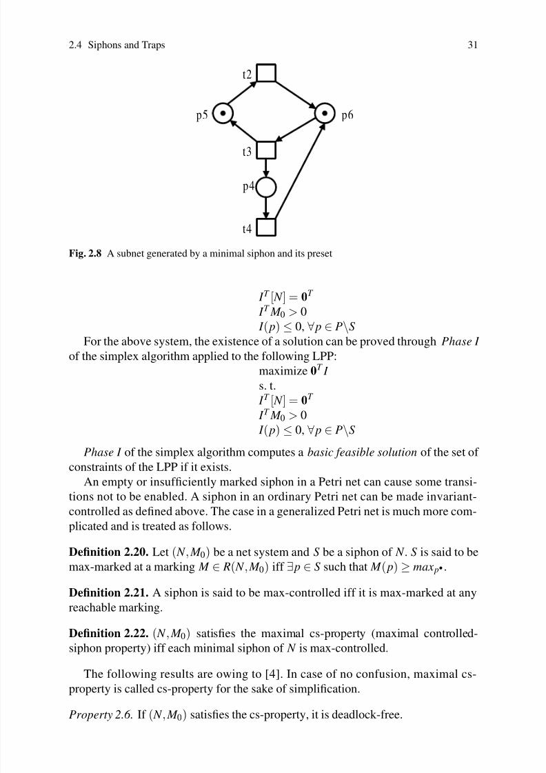
8/4/2019 Li Z., Zhou M. Deadlock Resolution in Automated Manufacturing Systems - A Novel Petri Net Approach
http://slidepdf.com/reader/full/li-z-zhou-m-deadlock-resolution-in-automated-manufacturing-systems-a-novel 48/249
2.4 Siphons and Traps 31
t 2
t 3
p 5
t 4
p 4
p 6
Fig. 2.8 A subnet generated by a minimal siphon and its preset
I T [ N ] = 0T
I T M 0 > 0
I ( p) ≤ 0, ∀ p ∈ P\S
For the above system, the existence of a solution can be proved through Phase I
of the simplex algorithm applied to the following LPP:
maximize 0T I
s. t.
I
T
[ N ] =0T
I T M 0 > 0
I ( p) ≤ 0, ∀ p ∈ P\S
Phase I of the simplex algorithm computes a basic feasible solution of the set of
constraints of the LPP if it exists.
An empty or insufficiently marked siphon in a Petri net can cause some transi-
tions not to be enabled. A siphon in an ordinary Petri net can be made invariant-
controlled as defined above. The case in a generalized Petri net is much more com-
plicated and is treated as follows.
Definition 2.20. Let ( N , M 0) be a net system and S be a siphon of N . S is said to be
max-marked at a marking M ∈ R( N , M 0) iff ∃ p ∈ S such that M ( p) ≥ max p• .
Definition 2.21. A siphon is said to be max-controlled iff it is max-marked at any
reachable marking.
Definition 2.22. ( N , M 0) satisfies the maximal cs-property (maximal controlled-
siphon property) iff each minimal siphon of N is max-controlled.
The following results are owing to [4]. In case of no confusion, maximal cs-property is called cs-property for the sake of simplification.
Property 2.6. If ( N , M 0) satisfies the cs-property, it is deadlock-free.

8/4/2019 Li Z., Zhou M. Deadlock Resolution in Automated Manufacturing Systems - A Novel Petri Net Approach
http://slidepdf.com/reader/full/li-z-zhou-m-deadlock-resolution-in-automated-manufacturing-systems-a-novel 49/249
32 2 Petri Nets
Property 2.7. If ( N , M 0) is live, it satisfies the cs-property.
A siphon satisfying the max-controlled property can be always marked suffi-
ciently to allow firing a transition once at least. In order to check and use the cs-
property, Barkaoui et al. [4] propose the conditions to determine whether a given
siphon is max-controlled.
Proposition 2.1. Let ( N , M 0) be a Petri net and S be a siphon of N. If there ex-
ists a P-invariant I such that ∀ p ∈ (|| I ||− ∩ S) , max p• = 1 , || I ||+ ⊆ S and I T M 0 >
∑ p∈S I ( p)(max p• − 1) , then S is max-controlled.
Example 2.15. Figure 2.9a shows a generalized net and I 1 = p2 + p6 and I 2 = p2 + 3 p3 + p5 are its two P-invariants. Trivially, I = I 2 − I 1 = 3 p3 + p5 − p6 is also
a P-invariant. Let S = p3, p5 be a set of places. Since •S ⊂ S•, S is a strict mini-
mal siphon. Next we show that it is max-controlled by P-invariant I . It is clear that
|| I ||− ∩S = / 0 and || I ||+ = S. We then check the truth of I T M 0 >∑ p∈S I ( p)(max p• −1). I T M 0 = M 0( p5) + 3 M 0( p3) − M 0( p6) = 3 − 1 = 2. ∑ p∈S I ( p)(max p• − 1) = I ( p3)(max p•
3− 1) + I ( p5)(max p•
5− 1). Considering max p•
3= 1 and max p•
5= 2, we
have ∑ p∈S I ( p)(max p• − 1) = 1. Therefore, I T M 0 > ∑ p∈S I ( p)(max p• − 1) and S is
max-controlled. Figure 2.9b shows the reachability graph of the net in Fig. 2.9a.
p 1
p 5
p 3
p 4
p 2
t 1
t 3
t 22
3
p 6
( a )
M 0= 3 p1+ 2 p4+ 3 p5+ p 6
t 1
M 1= 2 p1+ p2+ 2 p4+ 2 p5
t 2
M 2= 2 p1+ p3+ p4+ p6
t 3
( b )
Fig. 2.9 A max-controlled siphon in a net ( N , M 0) (a) Petri net model and (b) reachability graph
By comparing the net in Fig. 2.9a with Fig 2.1a as well as their reachability
graphs as shown in Fig. 2.9b and Fig. 2.3, respectively, one concludes that the addi-
tion of p6 removes two markings M 3 and M 4 in Fig. 2.3: one is a deadlock marking
and the other is a marking that inevitably leads the system to deadlock.
Remark 2.1. The number of siphons (minimal siphons) grows fast with respect to the
size of a Petri net and in the worst case grows exponentially with a net size. However,
many deadlock control approaches depend on the complete or partial enumeration
of siphons in a plant net model [23, 33, 34, 40, 50–52, 58, 59]. It is well known that
the complete siphon enumeration is time-consuming. Extensive studies have been

8/4/2019 Li Z., Zhou M. Deadlock Resolution in Automated Manufacturing Systems - A Novel Petri Net Approach
http://slidepdf.com/reader/full/li-z-zhou-m-deadlock-resolution-in-automated-manufacturing-systems-a-novel 50/249
2.5 Subclasses of Petri Nets 33
conducted on the siphon computation, leading to a variety of methods [1,14,22,31,
35, 53, 54]. A recent work [15] by Cordone et al. claims that their proposed siphon
computation method can find more than 2×10⁷ siphons in less than one hour.
2.5 Subclasses of Petri Nets
There are a number of interesting subclasses of ordinary Petri nets. The reasons that
they are interesting are twofold. First, they play an important role in the develop-
ment of certain application of Petri nets [11, 12]. Second, some relevant analysis
problems in these classes can be solved in polynomial time [3,21,36]. For example,
the problem of deciding whether a free-choice Petri net is live and bounded can be
solved in O(nm) [21], where n and m are the number of places and transitions of the
net, respectively. In turn, many analysis problems of live and bounded free-choice
nets are also shown to have polynomial time complexity [16].
Definition 2.23. A Petri net N = (P,T ,F ) is called a state machine iff ∀ t ∈ T , |•t | =|t •| = 1.
In a state machine, each transition has exactly one input place and exactly one
output place. Each transition allows tokens to flow from one place to another. Mul-
tiple transitions may allow tokens to flow from their respective places to the same
place. In addition, a single token in a place p enables all transitions in p•. Firing anyof them disables the others. This is called a conflict. Note that all finite automata
can be described as the state machines of Petri nets.
Theorem 2.6. A state machine ( N , M 0) is live iff N is strongly connected and M 0marks at least one place.
Definition 2.24. A Petri net N = (P,T ,F ) is said to be a marked graph iff ∀ p ∈ P,
|• p| = | p•| = 1.
In a marked graph, each place has exactly one input transition and exactly one
output transition. A transition may have multiple input places and output places. In
this sense, a marked graph allows concurrent and synchronization structure. A state
machine admits no synchronization and a marked graph allows no conflict.
Theorem 2.7. A marked graph ( N , M 0) is live iff M 0 places at least one token on
each circuit in N.
Definition 2.25. A Petri net is a free-choice net iff ∀ p1, p2 ∈ P, p•1 ∩ p•
2 = / 0 ⇒ | p•1| =
| p•2| = 1.
In a free-choice net, every arc from a place is either a unique outgoing arc or
a unique incoming arc to a transition. A free-choice net allows both conflict and
synchronization, i.e., state machines and marked graphs fall under the class of free-
choice nets.

8/4/2019 Li Z., Zhou M. Deadlock Resolution in Automated Manufacturing Systems - A Novel Petri Net Approach
http://slidepdf.com/reader/full/li-z-zhou-m-deadlock-resolution-in-automated-manufacturing-systems-a-novel 51/249
34 2 Petri Nets
Theorem 2.8. A free-choice net ( N , M 0) is live iff every siphon in it contains a
marked trap.
Definition 2.26. A Petri net is an extended free-choice net iff ∀ p1, p2 ∈ P, p•1 ∩ p•
2 = / 0
⇒p•
1
= p•2
.
Definition 2.27. A Petri net is an asymmetric choice net iff ∀ p1, p2 ∈ P, p•1 ∩ p•
2 = / 0 ⇒ p•
1 ⊆ p•2 or p•
2 ⊆ p•1.
Theorem 2.9. An asymmetric choice net ( N , M 0) is live if (but not only if) every
siphon in N contains a marked trap.
Example 2.16. Figure 2.10 shows some subclasses of Petri nets.
( a )
( f )( c )
( e )
( d )
( b )
Fig. 2.10 Subclasses of Petri nets: (a) a state machine but not marked graph, (b) a marked graph
but not state machine, (c) a free-choice net, (d) an extended free-choice net, (e) an asymmetric net,
and (f) a Petri net
2.6 Petri Nets and Automata
Since the reachability graph of a Petri net is an automaton, this section presents
some basics of finite-state automata [26], which are helpful to understand what is
presented in this book.

8/4/2019 Li Z., Zhou M. Deadlock Resolution in Automated Manufacturing Systems - A Novel Petri Net Approach
http://slidepdf.com/reader/full/li-z-zhou-m-deadlock-resolution-in-automated-manufacturing-systems-a-novel 52/249
2.6 Petri Nets and Automata 35
Definition 2.28. A (deterministic) finite-state automaton is a 5-tuple G = (Q, Σ , δ ,q0, Qm), where Q is a finite set of states, Σ is a finite alphabet of symbols that we
refer to as event labels, δ : Q×Σ the (partial) transition function, q0 the initial state,
and Qm ⊆ Q the set of marker states.
δ is a partial function since δ (q,α ) may not be defined for all (q,α ) ∈ Q ×Σ .When δ (q,α ) is defined, it implies that ∃ q′ ∈ Q and α ∈ Σ , the occurrence of event
α transits the automaton from states q to q′.
q2
b
q1q0 a , b
a a
b
Fig. 2.11 An automaton
The operation of a finite-state automaton is always illustrated in a state diagram.
Graphically, the initial state is marked with an input arrow and the marker states
are denoted by double circles. For instance, Figure 2.11 shows an automaton G,
where Q = q0,q1,q2, Σ = a,b, the initial state is q0, Qm = q1, δ (q0,b) = q0,
δ (q0,a) = q1, δ (q1,b) = q1, δ (q1,a) = q2, δ (q2,a) = q1, and δ (q2,b) = q1.
The behavior of a system modeled by an automaton can be characterized by the
language that the automaton speaks, i.e., a set of sequences of symbols of events
from Σ , which are physically possible. For example, σ = abab is a possible se-
quence of events in the automaton in Fig. 2.11. The set of all finite sequences over
Σ is denoted by Σ ∗, which includes the empty string whose length is zero and which
is denoted by ε .
Definition 2.29. A labeled Petri net is a net with a labeling function l : T →2Σ
∪ε
, where Σ is the set of events and ε is a null event. A net is said to be
free-labeled if each transition t ∈ T is labeled by a single event a ∈ Σ and differenttransitions bear different labels.
The reachability graph of a free-labeled Petri net corresponds to a deterministic
automaton. A finite automaton can easily be converted into a labeled Petri net by
inserting a transition that is labeled by the symbol between two connected states.
The states in the automaton are differently numbered by places. Figure 2.12 is the
equivalent labeled Petri net of the automaton depicted in Fig. 2.11.
For supervisory control of DES in a Petri net formalism, we are more concerned
with a free-labeled Petri net representation. Unfortunately, it is shown that not allfinite automata admit a free-labeled Petri net representation. It remains unanswered
what finite automata do have a free-labeled Petri net realization. Figure 2.13 shows
two finite automata that have no such realizations.
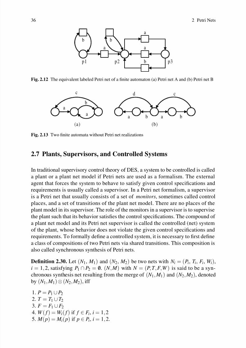
8/4/2019 Li Z., Zhou M. Deadlock Resolution in Automated Manufacturing Systems - A Novel Petri Net Approach
http://slidepdf.com/reader/full/li-z-zhou-m-deadlock-resolution-in-automated-manufacturing-systems-a-novel 53/249
36 2 Petri Nets
b
b p 3
b
p 2p 1
aa
a
Fig. 2.12 The equivalent labeled Petri net of a finite automaton (a) Petri net A and (b) Petri net B
c
ba
ab a
( a )
a
cd
b
( b )
Fig. 2.13 Two finite automata without Petri net realizations
2.7 Plants, Supervisors, and Controlled Systems
In traditional supervisory control theory of DES, a system to be controlled is called
a plant or a plant net model if Petri nets are used as a formalism. The external
agent that forces the system to behave to satisfy given control specifications andrequirements is usually called a supervisor. In a Petri net formalism, a supervisor
is a Petri net that usually consists of a set of monitors, sometimes called control
places, and a set of transitions of the plant net model. There are no places of the
plant model in its supervisor. The role of the monitors in a supervisor is to supervise
the plant such that its behavior satisfies the control specifications. The compound of
a plant net model and its Petri net supervisor is called the controlled (net) system
of the plant, whose behavior does not violate the given control specifications and
requirements. To formally define a controlled system, it is necessary to first define
a class of compositions of two Petri nets via shared transitions. This composition isalso called synchronous synthesis of Petri nets.
Definition 2.30. Let ( N 1, M 1) and ( N 2, M 2) be two nets with N i = (Pi, T i, F i, W i),
i = 1,2, satisfying P1 ∩ P2 = / 0. ( N , M ) with N = (P,T ,F ,W ) is said to be a syn-
chronous synthesis net resulting from the merge of ( N 1, M 1) and ( N 2, M 2), denoted
by ( N 1, M 1)⊗ ( N 2, M 2), iff
1. P = P1 ∪ P2
2. T = T 1
∪T 2
3. F = F 1 ∪ F 24. W ( f ) = W i( f ) if f ∈ F i, i = 1,2
5. M ( p) = M i( p) if p ∈ Pi, i = 1,2.

8/4/2019 Li Z., Zhou M. Deadlock Resolution in Automated Manufacturing Systems - A Novel Petri Net Approach
http://slidepdf.com/reader/full/li-z-zhou-m-deadlock-resolution-in-automated-manufacturing-systems-a-novel 54/249
2.8 Bibliographical Remarks 37
Definition 2.31. Let ( N 1, M 1), ( N 2, M 2), . . ., and ( N k , M k ) be k nets satisfying Pi ∩P j = / 0, ∀i, j ∈ Nk , i = j. The synchronous synthesis of the k Petri nets ( N 1, M 1),
( N 2, M 2), . . ., and ( N k , M k ) is defined as ( N , M ) = ( N k , M k ) ⊗ (⊗k −1i=1 ( N i, M i)).
In a Petri net formalism, a supervisor is a Petri net that usually consists of a set
of monitors and a set of transitions, which is a subset of the set of transitions in the
plant net model. The controlled system is the synchronous synthesis of a plant net
model and its supervisor via shared transitions.
Definition 2.32. Let ( N p, M p) with N p = (P,T ,F ,W ) be a plant model and ( N sup,
M sup) with N sup = (PV ,T V ,F V ,W V ) its supervisor, where P ∩ PV = / 0 and T V ⊆ T .
The controlled system of the plant model is ( N p, M p) ⊗ ( N sup, M sup).
Example 2.17. The Petri net shown in Fig. 2.14a is a plant model. The control spec-
ification is that the number of tokens in place p2 is not greater than one at anyreachable marking. The net depicted in Fig. 2.14b is a supervisor that can imple-
ment this control specification, where p3 is a monitor, PV = p3, and T V = t 1,t 2.
Figure 2.14c shows the controlled system that can be obtained by synchronous syn-
thesis of the nets in Fig. 2.14a, b. It is easy to verify that the number of tokens in p2
can never be greater than one.
p 3
t 1
t 2
( b )
p 1 p 2
t 1
t 2
( a )
p 1 p 3p 2
t 1
t 2
( c )
Fig. 2.14 (a) a plant net model, (b) the supervisor, and (c) the controlled system
2.8 Bibliographical Remarks
All the material covered in this chapter can be found in standard books [16, 39,
43] and survey papers [37, 38]. A good paper on siphons is [2], which presents an
effective characterization of minimal siphons and traps from the viewpoint of graph
theory. The algorithms calculating siphons and traps can be found in [5,9,10,14,15,22, 29, 31, 48, 54, 57, 60]. For a general introduction to the subclasses of Petri nets,
we refer readers to [37]. Good surveys of Petri nets from a system theory view can
be found in [24, 46].

8/4/2019 Li Z., Zhou M. Deadlock Resolution in Automated Manufacturing Systems - A Novel Petri Net Approach
http://slidepdf.com/reader/full/li-z-zhou-m-deadlock-resolution-in-automated-manufacturing-systems-a-novel 55/249
38 2 Petri Nets
For a more extensive discussion of the original framework of DES supervisory
control based on formal languages and automata, we refer readers to the tutorial
surveys, papers and books [7,8,25,27,30,41,49].
Problems
2.1. It is known that the siphons are closely related to the deadlock or the existence
of dead transitions in a Petri net. Suppose that ( N , M 0) is a net without siphons. Is it
live? Results can be found in [55].
2.2. INA [47] is a widely used tool that supports the behavioral and structural anal-
ysis of Petri nets. Let us define the size of a net ( N , M 0) as
||N
||=
|P
|+
|T
|+
∑ p∈P M 0( p). By using INA, compute the reachability graphs for a number of Petrinets with different sizes 5, 10, 20, . . ., and 100, and observe the relationship between
the CPU-time and the size of a Petri net.
2.3. Figure 2.15 shows the reduced version of the reachability graph of the net in
Fig. 2.1a. It is clear that M 4 is a deadlock marking and M 3 is a marking that definitely
leads the system to a deadlock state. These are “bad” states , which the system is
not allowed to enter. M 1 is called a dangerous marking since, at this marking, the
system may enter M 3 if supervisory control is not properly imposed.
Therefore, M 0, M 1, and M 2 form the good behavior of the system. An intuitiveidea is to design an online supervisor that supervises the system such that if the
system reaches M 1, it disables t 1 and directs the system to M 2.
Combining with the results for Problem 2.2, discuss the disadvantages of this
intuitive control idea. Try to implement this idea by some programming language
and check the size of the problem that can be processed by your computer.
M 0
M 4
M 3M 2
M 1
t 1
t 1
t 1
t 3
t 2
Fig. 2.15 A reachability graph

8/4/2019 Li Z., Zhou M. Deadlock Resolution in Automated Manufacturing Systems - A Novel Petri Net Approach
http://slidepdf.com/reader/full/li-z-zhou-m-deadlock-resolution-in-automated-manufacturing-systems-a-novel 56/249
2.8 Bibliographical Remarks 39
2.4. Prove Corollary 2.3.
2.5. Find and compare the strict minimal siphons in Fig 2.16a, b. Change the ini-
tial markings of places p1 and p4 and verify the liveness of the two nets by INA.
This verification may find an interesting problem about deadlocks and siphons in a
generalized Petri net.
p 1
p 3
p 2
t 3
t 2
p 5
p 6
t 6
t 4
t 51 5
t 1
1 5
p 4p 8
p 7
6
42
4
4
4
4
2
( a )
p 1
p 3
p 2
t 3
t 2
p 5
p 6
t 6
t 4
t 51 5
t 1
1 5
p 4p 8
p 7
6
4
( b )
Fig. 2.16 Two Petri nets (a) a generalized one and (b) an ordinary one
2.6. The reachability graph of a Petri net ( N , M 0) can be constructed using the fol-
lowing algorithm that terminates in a finite number of steps if its reachability set is
finite. Starting with M 0, all the enabled transitions can be fired. These firings can
lead to new markings that may enable other transitions. Taking each of the new
markings as a new root, we can recursively generate all the reachable markings. The
following reachability graph generation algorithm can be found in [37, 39].
Algorithm 2.1 Reachability graph
1: The root node is M 0. This node has initially no label.
2: while There are nodes with no label do3: Consider a node M with no label.
4: (a) For each transition t enabled at M :
5: Let M ′ = M + [ N ](·, t ).
6: if There does not exist a node M ′ in the graph then
7: Add it.
8: Add an arc t from M to M ′.9: end if
10: (b) Label the node M “old”.
11: end while12: Remove all labels from nodes.
Implement the algorithm in a programming language and find the reachability
graphs for all the Petri nets in Chap. 2 and those used in Problem 2.2. Check the

8/4/2019 Li Z., Zhou M. Deadlock Resolution in Automated Manufacturing Systems - A Novel Petri Net Approach
http://slidepdf.com/reader/full/li-z-zhou-m-deadlock-resolution-in-automated-manufacturing-systems-a-novel 57/249
40 2 Petri Nets
maximal size of a reachability graph that your computer can process in reasonable
time. Compare the CPU-times needed by your program and INA.
Let M , M ′ ∈ R( N , M 0) be two reachable markings of a Petri net ( N , M 0) with
N = (P,T ,F ,W ). M is said to cover M ′ if M ≥ M ′, i.e., ∀ p ∈ P, M ( p) ≥ M ′( p).
For an unbounded Petri net, its reachability graph can grow indefinitely. To re-duce and keep the size of the graph finite, a special symbol ω is usually introduced,
which represents a number of tokens that can be made arbitrarily large. For any
finite integer a, ω is subject to the following four rules:
a ≤ ω ,ω ≤ ω ,ω + a = ω ,ω −a = ω .By using the above notations, a special graph called a coverability graph can be
constructed using the algorithm stated in [19]. If there is no symbolω in a graph, it is
also a reachability graph. A coverability graph is finite and contains every reachable
marking from an initial marking M 0, which is either explicitly represented by a node,
or is covered by a node through the use of ω . For details, the reader can be referred
to [19] and [37].
Additional work related to the check of liveness of unbounded Petri nets can be
found in [20, 28, 45, 56]. The liveness analysis problem of generalized unbounded
Petri nets remains open.
References
1. Abdallah, I.B., ElMaraghy, H.A., ElMekkawy, T. (1997) A logic programming approach for
finding minimal siphons in S3PR nets applied to manufacturing systems. In Proc. IEEE Int.
Conf. on Systems, Man, and Cybernetics, pp.1710–1715.2. Barkaoui, K., Lemaire, B. (1989) An effective characterization of minimal deadlocks and
traps in Petri nets based on graph theory. In Proc. 10th Int. Conf. on Applications and Theory
of Petri Nets, pp.1–21.3. Barkaoui, K., Minoux, M. (1992) A polynomial time graph algorithm to decide liveness of
some basic classes of Petri nets. In Proc. 13th Int. Conf. on Applications and Theory of Petri Nets, Lecture Notes in Computer Science, vol.616, pp.62–75.4. Barkaoui, K., Pradat-Peyre, J.F. (1996) On liveness and controlled siphons in Petri nets. In
Proc. 17th Int. Conf. on Applications and Theory of Petri Nets Lecture Notes in Computer
Science, vol.1091, pp.57–72.5. Boer, E.R., Murata, T. (1994) Generating basis siphons and traps of Petri nets using the sign
incidence matrix. IEEE Transactions on Circuits and Systems I–Fundamental Theory and
Applications, vol.41, no.4, pp.266–271.6. Bogdan, S., Lewis, F.L., Kovacic, Z., Mireles, J. (2006) Manufacturing Systems Control De-
sign. London: Springer.7. Cassandras, C.G., Lafortune, S. (1999) Introduction to Discrete Event Systems. Boston, MA:
Kluwer.8. Cassandras, C.G., Lafortune, S. (2008) Introduction to Discrete Event Systems. Springer.9. Chao, D.Y. (2006) Computation of elementary siphons in Petri nets for deadlock control.
Computer Journal, vol.49, no.4, pp.470–479.10. Chao, D.Y. (2006) Searching strict minimal siphons for SNC-based resource allocation sys-
tems, Journal of Information Science and Engineering, vol.23, no.3, pp.853–867.

8/4/2019 Li Z., Zhou M. Deadlock Resolution in Automated Manufacturing Systems - A Novel Petri Net Approach
http://slidepdf.com/reader/full/li-z-zhou-m-deadlock-resolution-in-automated-manufacturing-systems-a-novel 58/249
References 41
11. Cheung, K.S. (2004) New characterization for live and reversible augmented Petri nets. In-
formation Processing Letters, vol.92, no.5, pp.239–243.
12. Chu, F., Xie, X.L. (1997) Deadlock analysis of Petri nets using siphons and mathematical
programming. IEEE Transactions on Robotics and Automation, vol.13, no.6, pp.793–804.
13. Colom, J.M., Campos, J., Silva, M. (1990) On liveness analysis through linear algebraic tech-
niques. In Proc. of Annual General Meeting of ESPRIT Basic Research Action 3148 Design Methods Based on Nets DEMON .
14. Cordone, R., Ferrarini, L., Piroddi, L. (2003) Some results on the computation of minimal
siphons in Petri nets. In Proc. 42nd IEEE Conf. on Decision and Control, pp.3754–3759.
15. Cordone, R., Ferrarini, L., Piroddi, L. (2005) Enumeration algorithms for minimal siphons in
Petri nets based on place constraints. IEEE Transactions on Systems, Man and Cybernetics,
Part A, vol.35, no.6, pp.844–854.
16. Desel, J., Esparza, J. (1995) Free Choice Petri Nets. London: Cambridge University Press.
17. Desel, J., Reisig, W. (1998) Place/transition Petri nets. In Lectures on Petri Nets I: Basic
Models, Lecture Notes in Computer Science, vol.1491, W. Reisig and G. Rozenberg (Eds.),
pp.122–174.
18. Desel, J. (1998) Basic linear algebraic techniques for place/transition nets. In Lectures onPetri Nets I: Basic Models, Lecture Notes in Computer Science, vol.1491, W. Reisig and G.
Rozenberg (Eds.), pp.257–308.
19. Desrocher, A.A., AI-Jaar, R.Y. (1995) Applications of Petri Nets in Manufacturing Systems:
Modeling, Control, and Performance Analysis, Piscataway, NJ: IEEE Press.
20. Ding, Z.J., Jiang, C.J., Zhou, M.C. (2008) Deadlock checking for one-place unbounded Petri
nets based on modified reachability trees. IEEE Transactions on Systems, Man, and Cyber-
netics, Part B, vol.38, no.3, pp.881–882.
21. Esparza, J., Silva, M. (1992) A polynomial-time algorithm to decide liveness of bounded free
choice nets. Theoretical Computer Sciences, vol.102, no.1, pp.185–205.
22. Ezpeleta, J., Couvreur, J.M., Silva, M. (1993) A new technique for finding a generating family
of siphons, traps, and st-components: Application to colored Petri nets. In Advances in Petri
Nets, Lecture Notes in Computer Science, vol.674, G. Rozenberg (Ed.), pp.126–147.
23. Ezpeleta, J, Colom, J.M., Martinez, J. (1995) A Petri net based deadlock prevention policy
for flexible manufacturing systems. IEEE Transactions on Robotics and Automation, vol.11,
no.2, pp.173–184.
24. Giua, A., Seatzu, C. (2007) A systems theory view of Petri nets. In Advances in Control
Theory and Applications, Lecture Notes in Control and Information Science, vol.353, C.
Bonivento et al. (Eds.), pp.99–127.
25. Holloway, L.E., Krogh, B.H., Giua, A. (1997) A survey of Petri net methods for controlled
discrete event systems. Discrete Event Dynamic Systems: Theory and Applications, vol.7,
no.2, pp.151–190.
26. Hopcroft, J.E., Motwani, R., Ullman, J.D. (2000) Introduction to Automata Theory, Lan-
guages, and Computation, 2nd ed., New York: Addison-Wesley.
27. Hruz, B., Zhou, M.C (2007) Modeling and Control of Discrete-Event Dynamic Systems: With
Petri Nets and Other Tools. London: Springer.
28. Jeng, M.D, Peng, M.Y. (1999) Augmented reachability trees for 1-place-unbounded general-
ized Petri nets. IEEE Transactions on Systems, Man, and Cybernetics, Part A, vol.29, no.2,
pp.173–183.
29. Jeng, M.D., Peng, M.Y., Huang, Y.S. (1999) An algorithm for calculating minimal siphons
and traps in Petri nets. International Journal of Intelligent Control and Systems, vol.3, no.3,
pp.263–275.
30. Kumar, R. Garg, V. (1995) Modeling and Control of Logical Discrete Event Systems. Boston,
MA: Kluwer.
31. Lautenbach, K. (1987) Linear algebraic calculation of deadlocks and traps. In Concurrencyand Nets, K. Voss, H. J. Genrich and G. Rozenberg (Eds.), pp.315–336.
32. Lautenbach, K., Ridder, H. (1993) Liveness in bounded Petri nets which are covered by T-
invariants. In Proc. 13th Int. Conf. on Applications and Theory of Petri Nets, Lecture Notes in
Computer Science, vol.815, R. Valette (Ed.), pp.358–375.

8/4/2019 Li Z., Zhou M. Deadlock Resolution in Automated Manufacturing Systems - A Novel Petri Net Approach
http://slidepdf.com/reader/full/li-z-zhou-m-deadlock-resolution-in-automated-manufacturing-systems-a-novel 59/249
42 2 Petri Nets
33. Li, Z.W., Zhou, M.C. (2004) Elementary siphons of Petri nets and their application to dead-
lock prevention in flexible manufacturing systems. IEEE Transactions on Systems, Man, and
Cybernetics, Part A, vol.34, no.1, pp.38–51.
34. Li, Z.W., Wei, N. (2007) Deadlock control of flexible manufacturing systems via invariant-
controlled elementary siphons of Petri nets. International Journal of Advanced Manufactur-
ing Technology, vol.33, no.1–2, pp.24–35.35. Li, Z.W., Zhou, M.C. (2008) On siphon computation for deadlock control in a class of Petri
nets. IEEE Transactions on Systems, Man, and Cybernetics, A., vol.38, no.3, pp.667–679.
36. Minoux, M., Barkaoui, K. (1990) Deadlocks and traps in Petri nets as horn-satisfiability solu-
tions and some related polynomially solvable problems. Discrete Mathematics, vol.29, no.2–
3, pp.195–210.
37. Murata, T. (1989) Petri nets: Properties, analysis, and applications. Proceedings of the IEEE ,
vol.77, no.4, pp.541–580.
38. Peterson, J.L. (1977) Petri nets. Computing Surveys, vol.9, no.3, pp.223–252.
39. Peterson, J.L. (1981) Petri Net Theory and the Modeling of Systems. Englewood Cliffs, NJ:
Prentice-Hall.
40. Piroddi, L., Cordone, R., Fumagalli, I. (2008) Selective siphon control for deadlock preven-tion in Petri nets, IEEE Transactions on Systems, Man, and Cybernetics, Part A, vol. 38, no.
6, pp.1337–1348.
41. Ramadge, P., Wonham, W.M. (1989) The control of discrete event systems. Proceedings of
the IEEE , vol.77, no.1, pp.81–89.
42. Recalde, L., Teruel, E., Silva, M., (1998) On linear algebraic techniques for liveness analysis
of P/T systems. Journal of Circuits, Systems, and Computers, vol.8, no.1, pp.223–265.
43. Reisig, W. (1985) Petri Nets: An Introduction. New York: Springer.
44. Reutenauer, C. (1990) The Mathematics of Petri Nets. Translated by I. Varig, Englewood
Cliffs, NJ: Prentice-Hall.
45. Ru, Y., Wu, W.M., Hadjicostis, C.N. (2006) Comments on “A modified reachability tree ap-
proach to analysis of unbounded Petri nets”. IEEE Transactions on Systems, Man, and Cy-bernetics, Part B, vol.36, no.5, p.1210.
46. Silva, M., Teruel, E. (1996) A systems theory perspective of discrete event dynamic systems:
The Petri net paradigm. In P. Borne, J. C. Gentina, E. Craye, and S. El Khattabi, (Eds.),
Symposium on Discrete Events and Manufacturing Systems, IMACS Multiconference, Lille,
France, pp.1–12.
47. Starke, P. H. (2003) INA: Integrated Net Analyzer . http://www2.informatik.hu-berlin.de/ ∼star
ke/ina.html.
48. Tanimoto, S., Yamauchi, M., Watanabe, T. (1996) Finding minimal siphons in general Petri
nets. IEICE Transactions on Fundamentals, vol.E79-A, no.11, pp.1817–1824.
49. Thistle, J.G. (1996) Supervisory control of discrete event systems. Mathematical and Com-
puter and Modeling, vol.23, no.11–12, pp.25–53.50. Tricas, F., Garacıa-Valles, F., Colom, J.M., Ezpeleta, J. (1998) A partial approach to the prob-
lem of deadlocks in processes with resources. Research Report, GISI-RR-97-05, Departa-
mento de Informatica e Ingenierıa de Sistemas, Universidad de Zaragoza, Spain.
51. Tricas, F., Garcıa-Valles, F., Colom, J.M., Ezpeleta, J. (1998) A structural approach to the
problem of deadlock prevention in processes with shared resources. In Proc. 4th Workshop
on Discrete Event Systems, pp.273–278.
52. Tricas, F., Ezpeleta, J. (1999) A Petri net solution to the problem of deadlocks in systems of
processes with resources. In Proc. IEEE Int. Conf. on Emerging Technologies and Factory
Automation, pp.1047–1056.
53. Tricas, F., Ezpeleta, J. (2003) Some results on siphon computation for deadlock prevention in
resource allocation systems modeled with Petri nets. In Proc. IEEE Int. Conf. on EmergingTechnologies and Factory Automation, pp.322–329.
54. Tricas, F., Ezpeleta, J. (2006) Computing minimal siphons in Petri net models of resource
allocation systems: A parallel solution. IEEE Transactions on Systems, Man, and Cybernetics,
Part A, vol.36, no.3, pp.532–539.

8/4/2019 Li Z., Zhou M. Deadlock Resolution in Automated Manufacturing Systems - A Novel Petri Net Approach
http://slidepdf.com/reader/full/li-z-zhou-m-deadlock-resolution-in-automated-manufacturing-systems-a-novel 60/249
References 43
55. Tsuji, K., Murata, T. (1993) On reachability conditions for unrestricted Petri nets. In Proc.
IEEE Int. Symp. on Circuits and Systems, pp.2713–2716.
56. Wang, F.Y., Gao, Y.Q., Zhou, M.C. (2004) A modified reachability tree approach to analy-
sis of unbounded Petri nets. IEEE Transactions on Systems, Man, and Cybernetics, Part B,
vol.34, no.1, pp.303–308.
57. Watanabe, T., Yamauchi, M., Tanimoto, S. (1998) Extracting siphons containing specified setof places in Petri nets. In Proc. IEEE Int. Conf. on Systems, Man, and Cybernetics, pp.142–
147.
58. Xing, K.Y., Hu, B.S., Chen, H.X. (1996) Deadlock avoidance policy for Petri-net modelling
of flexible manufacturing systems with shared resources. IEEE Transactions on Automatic
Control, vol.41, no.2, pp.289–295.
59. Xing, K.Y., Hu, B.S. (2005) Optimal liveness Petri net controllers with minimal structures for
automated manufacturing systems. In Proc. IEEE Int. Conf. on Systems, Man and Cybernet-
ics, pp.282–287.
60. Yamauchi, M., Watanabe, T. (1999) Algorithms for extracting minimal siphons containing
specified places in a general Petri net. IEICE Transactions on Fundamentals, vol.E82-A,
no.11, pp.2566–2575.61. Zhou, M.C., DiCesare, F. (1991) Parallel and sequential exclusions for Petri net modeling for
manufacturing systems. IEEE Transactions on Robotics and Automation, vol.7, no.4, pp.515–
527.
62. Zhou, M.C., DiCesare, F. (1993) Petri Net Synthesis for Discrete Event Control of Manufac-
turing Systems. Boston, MA: Kluwer.

8/4/2019 Li Z., Zhou M. Deadlock Resolution in Automated Manufacturing Systems - A Novel Petri Net Approach
http://slidepdf.com/reader/full/li-z-zhou-m-deadlock-resolution-in-automated-manufacturing-systems-a-novel 61/249
Chapter 3
Elementary Siphons of Petri Nets
Abstract This chapter first presents the concepts of poor, rich, and equivalent
siphons and the related invariant-control theory. It then discusses elementary and
dependent siphons in a Petri net, which play a key role in the development of struc-
turally simple liveness-enforcing (Petri net) supervisors. Dependent siphons are fur-
ther divided into strongly and weakly dependent ones. Next, a more general result
on the control of a siphon is given. Later, it is shown that the controllability of a de-
pendent siphon can be ensured by supervising its elementary siphons via properly
setting their control depth variables. For well-initially-marked Petri nets that cover
most of the manufacturing-oriented Petri net models in the literature, it is shown that
strongly and weakly dependent siphons have identical controllability conditions. Fi-
nally, an elementary siphon identification algorithm for a deadlock control purpose
is presented.
3.1 Introduction
This chapter presents the concept of elementary and dependent siphons in a Petri
net as well as their controllability. Elementary siphons are a special class of struc-tural objects. Their development is motivated by the observation that the change of
the number of tokens in a siphon linearly depends on the token variation of a set of
other siphons. It is shown that a dependent siphon can be implicitly controlled by
properly supervising the number of tokens staying in its elementary siphons. Ele-
mentary siphons play an important role in the development of deadlock prevention
approaches that lead to structurally simple liveness-enforcing monitor-based super-
visors.
45

8/4/2019 Li Z., Zhou M. Deadlock Resolution in Automated Manufacturing Systems - A Novel Petri Net Approach
http://slidepdf.com/reader/full/li-z-zhou-m-deadlock-resolution-in-automated-manufacturing-systems-a-novel 62/249
46 3 Elementary Siphons of Petri Nets
3.2 Equivalent Siphons
In this section, we present the concept of equivalent siphons.
Definition 3.1. Let S ⊆ P be a subset of places of Petri net N = (P,T ,F ,W ). P-vector λ S is called the characteristic P-vector of S iff ∀ p ∈ S, λ S( p) = 1; otherwise
λ S( p) = 0.
Definition 3.2. ηS = [ N ]T λ S is called the characteristic T -vector of S, where [ N ]T is
the transpose of incidence matrix [ N ].
By the above definitions, ηT S = ∑ p∈S[ N ]( p, ·) is trivially true. The physical im-
plication of the T -vector of a subset of places is clear: ηS(t ) > 0 means that ηS(t )tokens are put into S after t fires; ηS(t ) = 0 indicates that the number of tokens in S
does not change after t fires; and ηS(t ) < 0 implies that |ηS(t )| tokens are removedfrom S after t fires.
p 1
p 3
t 4
t 3
p 4
p 2
p 6
p 5p 7
t 2
t 1
Fig. 3.1 A Petri net ( N , M 0)
Example 3.1. Let S1 = p1− p4, S2 = p2, p4, p6, S3 = p4− p6, and S4 = p4,
p6, p7 be subsets of places of the Petri net shown in Fig. 3.1. We have λ S1=
p1 + p2 + p3 + p4 (i.e., the space-saving version of vector (1 1 1 1 0 0 0)T ), λ S2=
p2 + p4 + p6, λ S3= p4 + p5 + p6, and λ S4
= p4 + p6 + p7. We have ηS1= 0T and
ηS2= 0T . This is not surprising since both λ S1
and λ S2are P-semiflows. Firing a
transition does not change their token count. In addition, it is easy to verify that
ηS3 = ηS4 = −t 1 + t 3. Firing t 1 removes a token from S3 and S4, respectively, while
firing t 3 adds a token to S3 and S4, respectively.
More specifically, take S3 = p4, p5, p6 as an example. Firing t 1 removes a token
from p6 and does not change the number of tokens in p4 and p5. Therefore, S3 loses
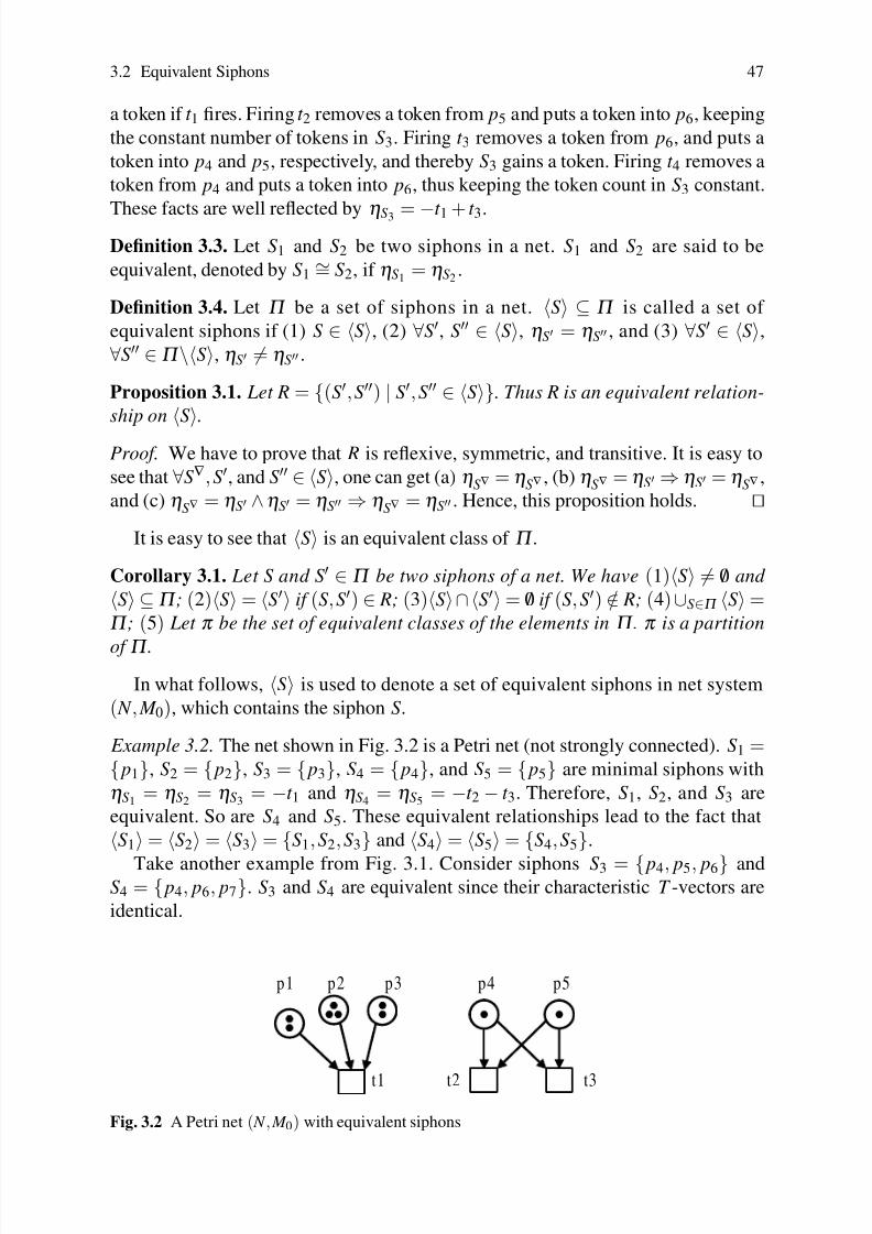
8/4/2019 Li Z., Zhou M. Deadlock Resolution in Automated Manufacturing Systems - A Novel Petri Net Approach
http://slidepdf.com/reader/full/li-z-zhou-m-deadlock-resolution-in-automated-manufacturing-systems-a-novel 63/249
3.2 Equivalent Siphons 47
a token if t 1 fires. Firing t 2 removes a token from p5 and puts a token into p6, keeping
the constant number of tokens in S3. Firing t 3 removes a token from p6, and puts a
token into p4 and p5, respectively, and thereby S3 gains a token. Firing t 4 removes a
token from p4 and puts a token into p6, thus keeping the token count in S3 constant.
These facts are well reflected by ηS3 = −t 1 + t 3.Definition 3.3. Let S1 and S2 be two siphons in a net. S1 and S2 are said to be
equivalent, denoted by S1∼= S2, if ηS1
= ηS2.
Definition 3.4. Let Π be a set of siphons in a net. S ⊆ Π is called a set of
equivalent siphons if (1) S ∈ S, (2) ∀S′, S′′ ∈ S, ηS′ = ηS′′ , and (3) ∀S′ ∈ S,
∀S′′ ∈Π \S, ηS′ = ηS′′ .
Proposition 3.1. Let R = (S′,S′′) | S′,S′′ ∈ S. Thus R is an equivalent relation-
ship on
S
.
Proof. We have to prove that R is reflexive, symmetric, and transitive. It is easy to
see that ∀S∇,S′, and S′′ ∈ S, one can get (a) ηS∇ = ηS∇ , (b) ηS∇ =ηS′ ⇒ηS′ = ηS∇ ,
and (c) ηS∇ = ηS′ ∧ηS′ = ηS′′ ⇒ ηS∇ = ηS′′ . Hence, this proposition holds. ⊓⊔It is easy to see that S is an equivalent class of Π .
Corollary 3.1. Let S and S′ ∈ Π be two siphons of a net. We have (1)S = / 0 and
S ⊆Π ; (2)S = S′ if (S,S′) ∈ R; (3)S∩S′ = / 0 if (S,S′) /∈ R; (4)∪S∈Π S =Π ; (5) Let π be the set of equivalent classes of the elements in Π . π is a partition
of Π .
In what follows, S is used to denote a set of equivalent siphons in net system
( N , M 0), which contains the siphon S.
Example 3.2. The net shown in Fig. 3.2 is a Petri net (not strongly connected). S1 = p1, S2 = p2, S3 = p3, S4 = p4, and S5 = p5 are minimal siphons with
ηS1= ηS2
= ηS3= −t 1 and ηS4
= ηS5= −t 2 − t 3. Therefore, S1, S2, and S3 are
equivalent. So are S4 and S5. These equivalent relationships lead to the fact that
S1 = S2 = S3 = S1,S2,S3 and S4 = S5 = S4,S5.
Take another example from Fig. 3.1. Consider siphons S3 = p4, p5, p6 andS4 = p4, p6, p7. S3 and S4 are equivalent since their characteristic T -vectors are
identical.
p 2
t 1
p 1
t 3t 2
p 5p 4p 3
Fig. 3.2 A Petri net ( N , M 0) with equivalent siphons

8/4/2019 Li Z., Zhou M. Deadlock Resolution in Automated Manufacturing Systems - A Novel Petri Net Approach
http://slidepdf.com/reader/full/li-z-zhou-m-deadlock-resolution-in-automated-manufacturing-systems-a-novel 64/249
48 3 Elementary Siphons of Petri Nets
Definition 3.5. Let S be a set of equivalent siphons in a Petri net ( N , M 0). Siphon
S′ ∈ S is said to be token-poor in S if ∄S′′ ∈ S such that M 0(S′′)< M 0(S′) holds.
It is called token-rich otherwise.
A token-poor siphon holds the smallest number of tokens at initial marking M 0
among a set of equivalent siphons. Clearly, among these equivalent siphons, alltoken-poor siphons have the same token count at M 0.
Theorem 3.1. M 0(S′) = M 0(S′′) if siphons S′ and S′′ are token-poor in S.
If siphons S1 and S2 are both token-rich in S, M 0(S1) = M 0(S2) is not necessar-
ily true. Recalling that a siphon is said to be controlled if it is always marked at any
reachable marking, we immediately have the following result.
Theorem 3.2. A token-rich siphon is controlled.
Proof. If S is token-rich, there must exist a siphon S′ ∈ S such that ηS′ = ηS and M 0(S) > M 0(S′) are true. Hence, firing any transition removes the same number of
tokens from S and S′. Let M ∈ R( N , M 0) be any reachable marking. We have two
subcases: M (S′) > 0 and M (S′) = 0.
If M (S′) > 0, then M (S) > M (S′) > 0. Thus S is marked.
If M (S′) = 0, then M (S) = M 0(S)− M 0(S′) > 0. It is easy to see, in this case, that
at any reachable marking M , no output transitions of S′ can be enabled and fire to
remove tokens from S and S′. Thus S remains to be marked. ⊓⊔Theorem 3.3. Let S′ and S′′ be two token-poor siphons in
S
. S′ is controlled iff S′′
is controlled.
Proof. Assume that S′ and S′′ are token-poor siphons in ( N , M 0), where N =(P,T ,F ,W ). Therefore, they have the identical characteristic T -vector and the same
number of initial tokens. ∀t ∈ T , the number of tokens removed from S′ equals that
from S′′ if t fires. The controllability of S′ means that the least number of tokens in
S′ is greater than 0. Hence, the least number of tokens staying in S′′ is also greater
than 0. S′′ is therefore controlled.
Similarly, we can prove that S′ is controlled if S′′ is so. ⊓⊔Theorem 3.4. If a token-poor siphon in S is controlled, all siphons in S arecontrolled.
Theorem 3.4 indicates that the controllability of a token-poor siphon in S is
sufficient for that of all others in S.
Example 3.3. In Fig. 3.2, S1 = p1 and S3 = p3 are token-poor and S2 = p2is token-rich since M 0(S1) = M 0(S3) = 2, and M 0(S2) = 3. S2 is controlled due to
Theorem 3.2 since it remains marked even if S1 and S3 are emptied. Also, ∀ M ∈ R( N , M 0), if M (S1) > 0, then M (S3) > 0 and M (S2) > 0 hold.
The concept of equivalent siphons is essential to the identification of the set of
elementary siphons in a net system for deadlock control purposes. The motivation
to propose the concept of elementary siphons is to control dependent siphons by
explicitly controlling their elementary siphons only.

8/4/2019 Li Z., Zhou M. Deadlock Resolution in Automated Manufacturing Systems - A Novel Petri Net Approach
http://slidepdf.com/reader/full/li-z-zhou-m-deadlock-resolution-in-automated-manufacturing-systems-a-novel 65/249
3.3 Elementary and Dependent Siphons 49
3.3 Elementary and Dependent Siphons
Theorems 3.3 and 3.4 show the controllability relations among equivalent siphons.
The concept of elementary and dependent siphons [20, 21] reveals the relations
among siphons belonging to different sets of equivalent siphons.
Definition 3.6. Let N = (P,T ,F ,W ) be a net with |P| = m, |T | = n and Π = S1,S2,
. . ., Sk be a set of siphons of N (m,n,k ∈N+). Let λ Si(ηSi
) be the characteristic
P(T )-vector of siphon Si, i ∈Nk . [λ ]k ×m = [λ S1|λ S2
| · · · |λ Sk ]T and [η]k ×n = [λ ]k ×m ×
[ N ]m×n = [ηS1|ηS2
| · · · |ηSk ]T are called the characteristic P- and T -vector matrices
of the siphons in N , respectively.
Definition 3.7. Let ηSα , ηSβ , . . ., and ηSγ (α ,β , . . . ,γ ⊆ Nk ) be a linearly inde-
pendent maximal set of matrix [η]. Then Π E =
Sα , Sβ , . . ., Sγ
is called a set of
elementary siphons in N .
Definition 3.8. S /∈ Π E is called a strongly dependent siphon if ηS = ∑Si∈Π E aiηSi
,
where ai ≥ 0.
Definition 3.9. S /∈Π E is called a weakly dependent siphon if ∃ A, B ⊂Π E , such that
A = / 0, B = / 0, A ∩ B = / 0, and ηS=∑Si∈ A aiηSi−∑Si∈ B aiηSi
, where ai > 0.
LetΓ +(S) =∑Si∈ A aiηSiandΓ −(S) =∑Si∈ B aiηSi
for a weakly dependent siphon
S. We have ηS = Γ +(S)−Γ −(S). If S is strongly dependent, we define Γ −(S) = 0.
Definition 3.10. Dependent siphons S1 and S2 are said to be quasi-equivalent iff
Γ +(S1) = Γ +(S2).
Lemma 3.1. The number of elements in any set of elementary siphons in net N
equals the rank of [η ].
Let Π E denote a set of the elementary siphons in a Petri net. Since the rank of [η]is at most the smaller of |P| and |T |, Lemma 3.1 leads to the following important
conclusion.
Theorem 3.5. |Π E | ≤ min|P|, |T |.
This result indicates that the number of elementary siphons in a Petri net is
bounded by the smaller of place count and transition count.
Let S be a (strongly or weakly) dependent siphon. In sequel, if ηS can be linearly
represented by elementary siphons’ characteristic T -vectors ηS1, ηS2
, . . ., and ηSn
with non-zero coefficients, we say that S1, S2, . . ., and Sn are the elementary siphons
of S. Let Π be the set of siphons in which we are interested given a net, and Π D be
the set of dependent ones within the scope of Π . Obviously, we have Π =Π E ∪Π D.
Example 3.4. The Petri net shown in Fig. 3.3(a) has 10 minimal siphons: S1 = p5,
p9, p12, p13, S2 = p4, p6, p13, p14, S3 = p6, p9, p12− p14, S4 = p2, p15,
S5 = p7, p11, S6 = p1− p3, p5− p7, S7 = p4, p8- p10, S8 = p3, p9, p12,

8/4/2019 Li Z., Zhou M. Deadlock Resolution in Automated Manufacturing Systems - A Novel Petri Net Approach
http://slidepdf.com/reader/full/li-z-zhou-m-deadlock-resolution-in-automated-manufacturing-systems-a-novel 66/249
50 3 Elementary Siphons of Petri Nets
S9 = p4, p5, p13, and S10 = p6, p8, p14. Each S4−S10 is both a siphon and trap.
Such a siphon cannot be emptied once it is initially marked. Now we consider the
strict minimal siphons S1, S2, and S3. We have
λ S1= p5 + p9 + p12 + p13,
λ S2 = p4 + p6 + p13 + p14,λ S3= p6 + p9 + p12 + p13 + p14,
ηS1= −t 2 + t 3 − t 9 + t 10,
ηS2= −t 3 + t 4 − t 8 + t 9,
ηS3= −t 2 + t 4 − t 8 + t 10.
Accordingly, [λ ] and [η] are shown as follows:
[λ ] =
⎛
⎝0 0 0 0 1 0 0 0 1 0 0 1 1 0 0
0 0 0 1 0 1 0 0 0 0 0 0 1 1 0
0 0 0 0 0 1 0 0 1 0 0 1 1 1 0
⎞
⎠,
[η ] =
⎛⎝ 0 −1 1 0 0 0 0 0 −1 1 0
0 0 −1 1 0 0 0 −1 1 0 0
0 −1 0 1 0 0 0 −1 0 1 0
⎞⎠ .
It is easy to verify that ηS3=ηS1
+ηS2and the rank of [η] is two, i.e., rank ([η]) =
|Π E | = 2. This means that there are two elementary siphons. If S1 and S2 are selected
as elementary siphons, S3 is a strongly dependent one. If S1 and S3 are selected
as elementary ones, S2 becomes weakly dependent. If S2 and S3 are selected aselementary ones, S1 is weakly dependent.
3.4 Controllability of Dependent Siphons in Ordinary Petri Nets
This section mainly focuses on the development of conditions under which a de-
pendent siphon can be always marked if their elementary ones are controlled. The
results presented are useful in the design of liveness-enforcing net supervisors for
resource allocation systems.
Invariant-based siphon control is a well-established technique in the literature.
The concept of general-invariant-controlled siphons is an extension to the known
results in [9,15,19,32].
Let ( N , M 0) be a net system. S is a siphon and I is a P-invariant of N , where
S ∩ || I ||+ = / 0 and S ∩ || I ||− = / 0. Let S ∩ || I ||+ = A, || I ||+\S = B, and || I ||− = C .
Clearly, we have || I || = || I ||+ ∪|| I ||− = A ∪ B ∪C .
Definition 3.11. S is called general-invariant-controlled if
I T M 0 − max∑ p∈ B
I ( p) M ( p)+ min∑ p∈C
| I ( p)| M ( p) > 0,

8/4/2019 Li Z., Zhou M. Deadlock Resolution in Automated Manufacturing Systems - A Novel Petri Net Approach
http://slidepdf.com/reader/full/li-z-zhou-m-deadlock-resolution-in-automated-manufacturing-systems-a-novel 67/249
3.4 Controllability of Dependent Siphons in Ordinary Petri Nets 51
p 1
p 5
p 3
t 4
t 3
p 6
t 5
p 7
p 4
p 9
t 1 1
t 9
t 1 0
p 8
p 2
t 6
5
p 1 1
t 1
t 2
3
p 1 0
p 1 5
p 1 4
p 1 3
p 1 2
t 8
t 7
p 1
p 5
p 3
t 4
t 3
p 6
t 5
p 7
p 4
p 9
t 1 1
t 9
t 1 0
p 8
p 2
t 6
5
p 1 1
t 1
t 2
3
p 1 0
p 1 5
p 1 4
p 1 3
p 1 2
t 8
t 7
t 6t 1
t 9t 8
V S 2
t 8
t 1
V S 1t 6
t 1 0t 3
( b )
( a )
Fig. 3.3 (a) A Petri net ( N 1, M 1) and (b) its augmented net ( N 2, M 2)

8/4/2019 Li Z., Zhou M. Deadlock Resolution in Automated Manufacturing Systems - A Novel Petri Net Approach
http://slidepdf.com/reader/full/li-z-zhou-m-deadlock-resolution-in-automated-manufacturing-systems-a-novel 68/249
52 3 Elementary Siphons of Petri Nets
where M ∈ R( N , M 0).
Theorem 3.6. If siphon S is general-invariant-controlled, it is controlled.
Proof. Clearly, we have
|| I
||= A
∪ B
∪C .
∀ M
∈ R( N , M 0), I T M = I T M 0. As a result,
we have
∑ p∈ A
I ( p) M ( p) +∑ p∈ B
I ( p) M ( p) + ∑ p∈C
I ( p) M ( p) = I T M 0.
∑ p∈ A
I ( p) M ( p) = I T M 0 −∑ p∈ B
I ( p) M ( p) − ∑ p∈C
I ( p) M ( p)
= I T M 0 −∑ p∈ B
I ( p) M ( p) + ∑ p∈C
| I ( p)| M ( p)
≥ I T M 0 − max∑ p∈ B
I ( p) M ( p) + min∑ p∈C
| I ( p)| M ( p) > 0.
It is easy to see that
∑ p∈ A
I ( p) M ( p) > 0⇒
M (S) > 0.
As a result, we have M (S) > 0 if
I T M 0 − max∑ p∈ B
I ( p) M ( p)+ min∑ p∈C
| I ( p)| M ( p) > 0.
⊓⊔If a siphon is general-invariant-controlled by a P-invariant, it cannot be emptied,
i.e.,
∀ M
∈ R( N , M 0), it is marked under M . A general-invariant-controlled siphon in
an ordinary net system does not imply a potential deadlock.Due to a possibly large number of reachable markings in a net system ( N , M 0),
in general, it is difficult to solve max∑ p∈ B I ( p) M ( p) and min∑ p∈C | I ( p)| M ( p)since their solution requires the complete marking enumeration of ( N , M 0). Define
m B = max∑ p∈ B
I ( p) M ( p)| M = M 0 + [ N ]Y , M ≥ 0,Y ≥ 0
and
mC = min∑ p∈C
| I ( p)| M ( p)| M = M 0 + [ N ]Y , M ≥ 0,Y ≥ 0,

8/4/2019 Li Z., Zhou M. Deadlock Resolution in Automated Manufacturing Systems - A Novel Petri Net Approach
http://slidepdf.com/reader/full/li-z-zhou-m-deadlock-resolution-in-automated-manufacturing-systems-a-novel 69/249
3.4 Controllability of Dependent Siphons in Ordinary Petri Nets 53
where [ N ] is the incidence matrix and M and Y are vectors of real numbers. From
the basic theory of Petri nets, any reachable marking fulfils the state equation but
the converse is not true. Hence, we have
m B ≥ max∑ p∈ B I ( p) M ( p)| M ∈ R( N , M 0),and
mC ≤ min∑ p∈C
| I ( p)| M ( p)| M ∈ R( N , M 0).
Corollary 3.2. S is controlled if
I T M 0−
m B + mC > 0.
Proof. It is known that
m B ≥ max∑ p∈ B
I ( p) M ( p)
and
mC ≤ min∑ p
∈C
| I ( p)| M ( p).
Hence, I T M 0 − m B + mC > 0 implies the truth of
I T M 0 − max∑ p∈ B
I ( p) M ( p)+ min∑ p∈C
| I ( p)| M ( p) > 0.
⊓⊔The problem to find m B and mC is an LPP and can be solved in polynomial
time [26, 30]. As shown in [9], imposing integrity constraints to M and Y as it is
usually done in the literature significantly increases the computational complexity.If B = || I ||+ \ S = / 0, then || I ||+ ⊆ S. This immediately leads to the following
result.
Corollary 3.3. If || I ||+ \ S = / 0 , S is controlled if either
I T M 0 + min∑ p∈C
| I ( p)| M ( p) > 0
or
I T M 0 + mC > 0.

8/4/2019 Li Z., Zhou M. Deadlock Resolution in Automated Manufacturing Systems - A Novel Petri Net Approach
http://slidepdf.com/reader/full/li-z-zhou-m-deadlock-resolution-in-automated-manufacturing-systems-a-novel 70/249
54 3 Elementary Siphons of Petri Nets
Corollary 3.4. If || I ||+ \ S = / 0 , S is controlled if I T M 0 > 0.
Proof. Since min∑ p∈C | I ( p)| M ( p) ≥ 0, I T M 0 > 0 leads to the truth of
I T M 0 +
min∑ p∈C |
I ( p
)| M
( p
) >0.
By Corollary 3.3, S is controlled. ⊓⊔The concept of general-invariant-controlled siphons is useful to develop control-
lability conditions for dependent siphons since it is more general than invariant-
controlled siphons defined in Definition 2.19.
Let
M min(S) = min M (S)| M ∈ R( N , M 0) (3.1)and
M max(S) = max M (S)| M ∈ R( N , M 0). (3.2)
The linear dependency of the T -vector of a dependent siphon on those T -
vectors of its elementary siphons reveals the relationship between its and their token
changes. That is to say, the number of tokens in a dependent siphon can be controlled
by supervising the token flow in its elementary siphons.
Without loss of generality, we assume that in a Petri net ( N , M 0
), a strongly de-
pendent S satisfies ηS = ∑ni=1 aiηSi
, ai > 0, i ∈ Nn, and a weakly dependent siphon
S satisfies ηS = ∑ni=1 aiηSi
−∑m j=n+1 a jηS j
, ai > 0, i ∈ Nm. Concerning the control-
lability of a dependent siphon, we have the following results.
Theorem 3.7. A weakly dependent siphon S is controlled if
M 0(S) >n
∑i=1
ai( M 0(Si) − M min(Si))−m
∑ j=n+1
a j( M 0(S j) − M max(S j)). (3.3)
Proof. Since
ηS =n
∑i=1
aiηSi−
m
∑ j=n+1
a jηS j,
we have
λ T S [ N ] =
n
∑i=1aiλ
T Si [ N ]−
m
∑ j=n+1a jλ
T S j [ N ],
i.e.,

8/4/2019 Li Z., Zhou M. Deadlock Resolution in Automated Manufacturing Systems - A Novel Petri Net Approach
http://slidepdf.com/reader/full/li-z-zhou-m-deadlock-resolution-in-automated-manufacturing-systems-a-novel 71/249
3.4 Controllability of Dependent Siphons in Ordinary Petri Nets 55
(λ S −n
∑i=1
aiλ Si+
m
∑ j=n+1
a jλ S j)T [ N ] = 0T .
Let I = λ S −∑ni=1 aiλ Si
+∑m j=n+1 a jλ S j
. There are hence two subcases: (a) I is a
P-invariant and (b) I = 0.First we consider that
I = λ S −n
∑i=1
aiλ Si+
m
∑ j=n+1
a jλ S j
is a P-invariant of N . ∀ M ∈ R( N , M 0), we have I T M = I T M 0. Therefore, the follow-
ing equation holds by noting M (S′) = λ T S′ M , ∀S′ ∈Π , M ∈ R( N , M 0).
M (S) − n∑i=1
ai M (Si) + m∑
j=n+1
a j M (S j) = M 0(S) − n∑i=1
ai M 0(Si) + m∑
j=n+1
a j M 0(S j).
(3.4)
From (3.4), we have:
M (S) = M 0(S) −n
∑i=1
ai M 0(Si) +n
∑i=1
ai M (Si) +m
∑ j=n+1
a j M 0(S j) −m
∑ j=n+1
a j M (S j).
(3.5)
Obviously, S is controlled, i.e., M (S) > 0 if
M 0(S) >n
∑i=1
ai M 0(Si) −n
∑i=1
ai M (Si) −m
∑ j=n+1
a j M 0(S j) +m
∑ j=n+1
a j M (S j). (3.6)
Noticing ∀ M ∈ R( N , M 0), M min(S) ≤ M (S) and M max(S) ≥ M (S), (3.6) is true if
the following inequality holds.
M 0(S) >n
∑i=1
ai( M 0(Si) − M min(Si))− m
∑ j=n+1
a j( M 0(S j) − M max(S j)). (3.7)
As a result, S is controlled if
M 0(S) >n
∑i=1
ai( M 0(Si) − M min(Si))−m
∑ j=n+1
a j( M 0(S j) − M max(S j)).
Second, we consider the case of I = 0.
∀ M
∈ R( N , M 0), the following equation is
true.
M (S) −n
∑i=1
ai M (Si) +m
∑ j=n+1
a j M (S j) = 0.

8/4/2019 Li Z., Zhou M. Deadlock Resolution in Automated Manufacturing Systems - A Novel Petri Net Approach
http://slidepdf.com/reader/full/li-z-zhou-m-deadlock-resolution-in-automated-manufacturing-systems-a-novel 72/249
56 3 Elementary Siphons of Petri Nets
Thus, one concludes that M (S) > 0 if
n
∑i=1
ai M (Si) −m
∑ j=n+1
a j M (S j) > 0.
Since
M 0(S) −n
∑i=1
ai M 0(Si) +m
∑ j=n+1
a j M 0(S j) = 0,
M (S) > 0 if
M 0(S) −n
∑i=1
ai M 0(Si) +m
∑ j=n+1
a j M 0(S j) +n
∑i=1
ai M (Si) −m
∑ j=n+1
a j M (S j) > 0.
i.e.,
M 0(S) >n
∑i=1
ai( M 0(Si) − M min(Si))−m
∑ j=n+1
a j( M 0(S j) − M max(S j)).
Subcases (a) and (b) lead to the truth of the theorem.
⊓⊔
Corollary 3.5. A strongly dependent siphon S is controlled if
M 0(S) >n
∑i=1
ai( M 0(Si) − M min(Si)).
Definition 3.12. ( N , M 0) is said to be well-initially-marked iff ∀S ∈ Π , M max(S) = M 0(S).
This definition indicates that a siphon in a well-initially-marked Petri net has themaximal number of tokens at the initial marking. For example, the net in Fig. 3.3(a)
is well-initially-marked.
Corollary 3.6. Let ( N , M 0) be a well-initially-marked net system. A (strongly or
weakly) dependent siphon S is controlled if
M 0(S) >n
∑i=1
ai( M 0(Si) − M min(Si)).
Proof. It follows immediately due to Corollary 3.5 if S is a strongly dependent
siphon.
Let S be a weakly dependent siphon. From Theorem 3.7, it is controlled if

8/4/2019 Li Z., Zhou M. Deadlock Resolution in Automated Manufacturing Systems - A Novel Petri Net Approach
http://slidepdf.com/reader/full/li-z-zhou-m-deadlock-resolution-in-automated-manufacturing-systems-a-novel 73/249
3.4 Controllability of Dependent Siphons in Ordinary Petri Nets 57
M 0(S) >n
∑i=1
ai( M 0(Si) − M min(Si))−m
∑ j=n+1
a j( M 0(S j) − M max(S j)).
Since ∀S ∈Π , M max(S) = M 0(S), we have
m
∑ j=n+1
a j( M 0(S j) − M max(S j)) = 0.
This leads to the truth of the corollary.
⊓⊔The condition (∀S ∈ Π , M max(S) = M 0(S)) in a well-initially-marked net is rea-
sonable and meaningful in practice. As far as the authors know, this is true for
application-oriented Petri net subclasses in the literature, which can model flexiblemanufacturing systems, e.g., PPN [2], augmented marked graphs [9], S3PR [11],
L-S3PR [12], S4R [1], S4PR [28], ES3PR [14], WS3PSR [27], S∗PR [13], PNR
[17], RCN-merged nets [16], ERCN-merged nets [31], ERCN∗-merged nets [18],
S2LSPR [24], S3PGR2 [25], G-task [4], and G-system [33]. However, the verifica-
tion of the well-initially-markedness seems a formidable job given an arbitrary Petri
net.
By Theorem 3.7, in order to verify the controllability of a dependent siphon,
we need to compute M min(S) and M max(S), S ∈ Π E . M min(S) and M max(S) can be
obtained by solving problems (3.1) and (3.2), respectively. Due to a large number of
reachable markings, M min(S) and M max(S) are difficult to find. For this, we consider
M min(S) and M max(S) defined as follows by relaxing M and Y to any non-negative
real numbers.
Let
M min(S) = min M (S)| M = M 0 + [ N ]Y , M ≥ 0,Y ≥ 0
and
M max
(S) = max M (S)| M = M 0 + [ N ]Y , M ≥ 0,Y ≥ 0.Obviously, we have
M min(S) ≤ M min(S)
and
M max(S) ≥ M max(S).
Corollary 3.7. A weakly dependent siphon S is controlled if
M 0(S) >n
∑i=1
ai( M 0(Si) − M min(Si))−m
∑ j=n+1
a j( M 0(S j) − M max(S j)).
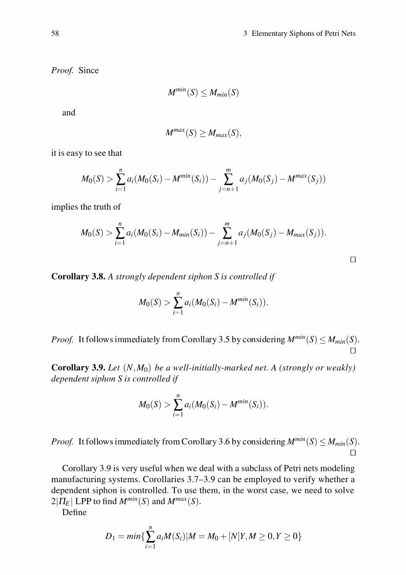
8/4/2019 Li Z., Zhou M. Deadlock Resolution in Automated Manufacturing Systems - A Novel Petri Net Approach
http://slidepdf.com/reader/full/li-z-zhou-m-deadlock-resolution-in-automated-manufacturing-systems-a-novel 74/249
58 3 Elementary Siphons of Petri Nets
Proof. Since
M min(S)
≤ M min(S)
and
M max(S) ≥ M max(S),
it is easy to see that
M 0(S) >n
∑i=1
ai( M 0(Si) − M min(Si))−m
∑ j=n+1
a j( M 0(S j) − M max(S j))
implies the truth of
M 0(S) >n
∑i=1
ai( M 0(Si) − M min(Si))−m
∑ j=n+1
a j( M 0(S j) − M max(S j)).
⊓⊔Corollary 3.8. A strongly dependent siphon S is controlled if
M 0(S) >
n
∑i=1ai( M 0(Si) − M
min
(Si)).
Proof. It follows immediately from Corollary 3.5 by considering M min(S) ≤ M min(S).
⊓⊔Corollary 3.9. Let ( N , M 0) be a well-initially-marked net. A (strongly or weakly)
dependent siphon S is controlled if
M 0(S) >
n
∑i=1
ai( M 0(Si) − M min(Si)).
Proof. It follows immediately from Corollary 3.6 by considering M min(S) ≤ M min(S).
⊓⊔Corollary 3.9 is very useful when we deal with a subclass of Petri nets modeling
manufacturing systems. Corollaries 3.7–3.9 can be employed to verify whether a
dependent siphon is controlled. To use them, in the worst case, we need to solve
2|Π E | LPP to find M min
(S) and M max
(S).Define
D1 = minn
∑i=1
ai M (Si)| M = M 0 + [ N ]Y , M ≥ 0,Y ≥ 0

8/4/2019 Li Z., Zhou M. Deadlock Resolution in Automated Manufacturing Systems - A Novel Petri Net Approach
http://slidepdf.com/reader/full/li-z-zhou-m-deadlock-resolution-in-automated-manufacturing-systems-a-novel 75/249
3.4 Controllability of Dependent Siphons in Ordinary Petri Nets 59
and
D2 = maxm
∑ j=n+1
a j M (S j)| M = M 0 + [ N ]Y , M ≥ 0,Y ≥ 0.
Next we present weaker conditions under which a dependent siphon can be con-
trolled.
Corollary 3.10. A weakly dependent siphon S is controlled if
M 0(S) >n
∑i=1
ai M 0(Si) − D1 −m
∑ j=n+1
a j M 0(S j) + D2.
Proof. From (3.6), S is controlled if
M 0(S) >n
∑i=1
ai M 0(Si) −n
∑i=1
ai M (Si) −m
∑ j=n+1
a j M 0(S j) +m
∑ j=n+1
a j M (S j).
Note that
D1 = minn
∑i=1
ai M (Si)| M = M 0 + [ N ]Y , M ≥ 0,Y ≥ 0 ≤n
∑i=1
ai M (Si)
and
D2 = maxm
∑ j=n+1
a j M (S j)| M = M 0 + [ N ]Y , M ≥ 0,Y ≥ 0 ≥m
∑ j=n+1
a j M (S j).
As a result, the truth of
M 0(S) >n
∑i=1
ai M 0(Si) − D1 −m
∑ j=n+1
a j M 0(S j) + D2
implies that of
M 0(S) >n
∑i=1
ai M 0(Si) −n
∑i=1
ai M (Si) −m
∑ j=n+1
a j M 0(S j) +m
∑ j=n+1
a j M (S j).
⊓⊔Corollary 3.11. Let S be a strongly dependent siphon in a net system ( N , M 0). S is
controlled if
M 0(S) >n
∑i=1
ai M 0(Si) − D1.

8/4/2019 Li Z., Zhou M. Deadlock Resolution in Automated Manufacturing Systems - A Novel Petri Net Approach
http://slidepdf.com/reader/full/li-z-zhou-m-deadlock-resolution-in-automated-manufacturing-systems-a-novel 76/249
60 3 Elementary Siphons of Petri Nets
Corollary 3.12. Let S be a (weakly or strongly) dependent siphon in a well-initially-
marked net ( N , M 0). S is controlled if
M 0(S) >n
∑i=1
ai M 0(Si)
− D1.
The controllability condition stated in Corollary 3.10 is weaker than that in
Corollary 3.7. However, its usage requires the computation of D1 and D2 for all de-
pendent siphons, which is time-consuming since the number of dependent siphons
is exponential with respect to the size of a net. For practical purposes, we can first
use Corollary 3.7 to verify the controllability of a dependent siphon. If it is not
controlled due to Corollary 3.7, Corollary 3.10 can be then employed. Our experi-
mental studies show that most controlled dependent siphons satisfy the condition in
Corollary 3.7.
Example 3.5. It is easy to verify that in net ( N 2, M 2) as shown in Fig. 3.3(b), I 1 = p5 − p7 − p8 + p9 + p12 + p13 −V S1
and I 2 = − p3 + p4 + p6 − p7 + p13 + p14 −V S2are
P-invariants of N 2. Clearly, S1 = p5, p9, p12, p13 is invariant-controlled by I 1 since
p| I 1( p) > 0 = S1 and I T 1 M 2 = M 2(S1)− M 2( p7)− M 2( p8)− M 2(V S1
) = 2−1 > 0,
where M 2 is an initial marking. Likewise, S2 is controlled by P-invariant I 2. Now we
check the controllability of S3, a strongly dependent siphon with respect to S1 and
S2 with ηS3= ηS1
+ηS2.
By solving LPP, we have M min(S1) = M min(S2) = 1. Note that M 2(S1) = 2,
M 2(S2) = 2, M 2(S3) = 3, and ∑2i=1( M 2(Si) − M
min
(Si)) = 2. Due to Corollary 3.9,S3 is controlled.
Remark 3.1. Compared with Fig. 3.3(a), places V S1and V S2
in Fig. 3.3(b) are used to
constrain the firing of transitions associated with siphons S1 and S2 respectively such
that M min(S1) = M min(S2) = 1, leading to the satisfaction of inequality M 2(S3) >
∑2i=1( M 2(Si) − M min(Si)).
When designing a liveness-enforcing supervisor for a plant, emptiable minimal
siphons in the plant model can be divided into elementary and dependent ones. Then
we can make the elementary siphons properly controlled by using an active siphon
control method, e.g., adding extra places like V S1and V S2
in Fig. 3.3(b). Therefore,
the dependent siphons can be implicitly controlled. In other words, if a plant Petri
net model contains emptiable siphons, it is possible for us to control only those
elementary ones. Since the number of elementary siphons is much smaller than
that of dependent siphons in most of large Petri nets, the concept of elementary
siphons can provide an effective way to prevent a large number of siphons from
being emptied by controlling only a small number of them.

8/4/2019 Li Z., Zhou M. Deadlock Resolution in Automated Manufacturing Systems - A Novel Petri Net Approach
http://slidepdf.com/reader/full/li-z-zhou-m-deadlock-resolution-in-automated-manufacturing-systems-a-novel 77/249

8/4/2019 Li Z., Zhou M. Deadlock Resolution in Automated Manufacturing Systems - A Novel Petri Net Approach
http://slidepdf.com/reader/full/li-z-zhou-m-deadlock-resolution-in-automated-manufacturing-systems-a-novel 78/249
62 3 Elementary Siphons of Petri Nets
p 3
p 1 1
p 1 2p 1
p 7
p 1 0
p 8
p 9
p 6
p 5
p 4
p 2
p 1 4
p 1 3
p 1 5
t 1
t 9
t 1 2
t 1 1
t 1 0
t 6
t 7
t 8
t 5
t 4
t 3
t 2
p 1 6
p 1 7
2
2
2
1 0 1 0
Fig. 3.4 A generalized Petri net ( N , M 0)
Theorem 3.8. A strongly dependent siphon S is max-controlled if
M 0(S) >
n
∑i=1 ai M 0(Si) −n
∑i=1 ai M min(Si) +ω (S).
Proof. Due to
ηS =n
∑i=1
aiηSi,
we have
λ T S [ N ] =
n
∑i=1
aiλ T Si
[ N ].
As a result,
(λ S −n
∑i=1
aiλ Si)T [ N ] = 0T .
Let
I = λ S −n
∑i=1
aiλ Si.

8/4/2019 Li Z., Zhou M. Deadlock Resolution in Automated Manufacturing Systems - A Novel Petri Net Approach
http://slidepdf.com/reader/full/li-z-zhou-m-deadlock-resolution-in-automated-manufacturing-systems-a-novel 79/249
3.5 Controllability of Dependent Siphons in Generalized Petri Nets 63
I = 0 or I is a P-invariant of N . According to the proof of Theorem 3.7, this
theorem is true in the case of I = 0. Next we consider that I is a P-invariant of N .
∀ M ∈ R( N , M 0), I T M = I T M 0. Therefore, we have
M 0(S) −n
∑i=1ai M 0(Si) = M (S) −
n
∑i=1ai M (Si),
M (S) = M 0(S) −n
∑i=1
ai M 0(Si) +n
∑i=1
ai M (Si),
and
M (S)≥
M 0(S)−
n
∑i=1
ai M 0(Si) +n
∑i=1
ai M min(Si).
Note that
M 0(S) >n
∑i=1
ai M 0(Si) −n
∑i=1
ai M min(Si) +ω (S).
It implies the truth of
M 0(S) −n
∑i=1 ai M 0(Si) +
n
∑i=1 ai M min(Si) > ω (S).
Hence, M (S) > ω (S). By Lemma 3.2, S is max-marked under M . Therefore,
∀ M ∈ R( N , M 0), S is max-marked under M . In other words, S is max-controlled if
M 0(S) >n
∑i=1
ai M 0(Si) −n
∑i=1
ai M min(Si) +ω (S).
⊓⊔ Example 3.7. There are three strict minimal siphons in Fig. 3.4. It is easy to verify
that S3 is a strongly dependent siphon with ηS3= ηS1
+ηS2.
In Fig. 3.5, we have M min(S1) = M min(S2) = 2. Considering that M 1(S1) = 5,
M 1(S2) = 4, M 1(S3) = 7, and ω (S3) = 1, M 1(S3) > ∑2i=1( M 1(Si) − M min(Si)) +
ω (S3) holds. As a result, S3 is max-controlled in Fig. 3.5 due to the existence of
monitors V S1and V S2
.
For the controllability of a weakly dependent siphon in a net system ( N , M 0), we
have the following results.
Theorem 3.9. A weakly dependent siphon S is max-controlled if
M 0(S) >n
∑i=1
ai( M 0(Si) − M min(Si))−m
∑ j=n+1
a j( M 0(S j) − M max(S j)) +ω (S).

8/4/2019 Li Z., Zhou M. Deadlock Resolution in Automated Manufacturing Systems - A Novel Petri Net Approach
http://slidepdf.com/reader/full/li-z-zhou-m-deadlock-resolution-in-automated-manufacturing-systems-a-novel 80/249
64 3 Elementary Siphons of Petri Nets
VS 2
t 1
t 9
t 1 1
t 6
t 2
2
2
2
VS 1
t 1t 9
t 1 0
t 7
t 3
p 3
p 1 1
p 1 2p 1
p 7
p 1 0
p 8
p 9
p 6
p 5
p 4
p 2
p 1 4
p 1 3
p 1 5
t 1
t 9
t 1 2
t 1 1
t 1 0
t 6
t 7
t 8
t 5
t 4
t 3
t 2
p 1 6
p 1 7
2
2
2
1 0 1 0
Fig. 3.5 A max-controlled siphon in a generalized Petri net ( N 1, M 1)
Proof. Since
ηS =n
∑i=1
aiηSi−
m
∑ j=n+1
a jηS j,
we have
λ T S [ N ] =
n
∑i=1
aiλ T Si
[ N ]−m
∑ j=n+1
a jλ T S j
[ N ],
and
(λ S −n
∑i=1
aiλ Si+
m
∑ j=n+1
a jλ S j)T [ N ] = 0T .
Let
I = λ S −n
∑i=1
aiλ Si+
m
∑ j=n+1
a jλ S j.
We have that I = 0 or I is a P-invariant of N . According to the proof of Theorem3.7, this theorem is true in the case of I = 0. Next we consider that I is a P-invariant
of N .

8/4/2019 Li Z., Zhou M. Deadlock Resolution in Automated Manufacturing Systems - A Novel Petri Net Approach
http://slidepdf.com/reader/full/li-z-zhou-m-deadlock-resolution-in-automated-manufacturing-systems-a-novel 81/249
3.5 Controllability of Dependent Siphons in Generalized Petri Nets 65
∀ M ∈ R( N , M 0), I T M = I T M 0. We have
M (S) −n
∑i=1
ai M (Si) +m
∑ j=n+1
a j M (S j)
= M 0(S) −n
∑i=1
ai M 0(Si) +m
∑ j=n+1
a j M 0(S j). (3.8)
From (3.8), we have
M (S) = M 0(S) −n
∑i=1
ai( M 0(Si) − M (Si)) +m
∑ j=n+1
a j( M 0(S j) − M (S j)). (3.9)
Clearly, the following inequality is true.
M (S) ≥ M 0(S)−n
∑i=1
ai( M 0(Si)− M min(Si)) +m
∑ j=n+1
a j( M 0(S j)− M max(S j)). (3.10)
From
M 0(S) >n
∑i=1
ai( M 0(Si) − M min(Si))−m
∑ j=n+1
a j( M 0(S j) − M max(S j)) +ω (S),
we have
M 0(S)−n
∑i=1
ai( M 0(Si)− M min(Si)) +m
∑ j=n+1
a j( M 0(S j)− M max(S j)) >ω (S). (3.11)
From (3.10) and (3.11), we have M (S) > ω (S) implying that S is max-marked
under M . Since M is any marking in R( N , M 0), S is max-controlled.
⊓⊔Corollary 3.13. A dependent siphon S in a well-initially-marked net ( N , M 0) is max-
controlled if
M 0(S) >n
∑i=1
ai( M 0(Si) − M min(Si)) +ω (S).
Proof. It is trivial if S is strongly dependent. Let S be weakly dependent in ( N , M 0).
Due to Theorem 3.9, S is max-controlled if
M 0(S) >n
∑i=1
ai( M 0(Si) − M min(Si))−m
∑ j=n+1
a j( M 0(S j) − M max(S j)) +ω (S).

8/4/2019 Li Z., Zhou M. Deadlock Resolution in Automated Manufacturing Systems - A Novel Petri Net Approach
http://slidepdf.com/reader/full/li-z-zhou-m-deadlock-resolution-in-automated-manufacturing-systems-a-novel 82/249
66 3 Elementary Siphons of Petri Nets
By Definition 3.12, ∀S ∈Π , M max(S) = M 0(S). As a result,
m
∑ j=n+1
a j( M 0(S j) − M max(S j)) = 0.
The controllability condition of a weakly dependent siphon coincides with that
of a strongly dependent one. ⊓⊔Corollary 3.14. A strongly dependent siphon S is max-controlled if
M 0(S) >n
∑i=1
ai M 0(Si) −n
∑i=1
ai M min(Si) +ω (S).
Proof. Since M min(S) ≤ M min(S),
M 0(S) >n
∑i=1
ai M 0(Si)−n
∑i=1
ai M min(Si) +ω (S)
⇒ M 0(S) >n
∑i=1
ai M 0(Si) −n
∑i=1
ai M min(Si) +ω (S).
⊓⊔Corollary 3.15. A weakly dependent siphon S is max-controlled if
M 0(S) >n
∑i=1
ai( M 0(Si) − M min(Si))−m
∑ j=n+1
a j( M 0(S j) − M max(S j)) +ω (S).
Corollary 3.16. A dependent siphon S in a well-initially-marked net system is max-
controlled if
M 0(S) >n
∑i=1
ai( M 0(Si)− M min(Si)) +ω (S).
From the above discussion, in order to verify the controllability of dependent
siphons, ∀i ∈N|Π E |, we need to compute M min(Si) and M max(Si) for Si. In the worst
case, we have to solve 2|Π E | LPP, where |Π E | is bounded by the structural size of a
net.
Recalling that
D1 = minn
∑i=1
ai M (Si)| M = M 0 + [ N ]Y , M ≥ 0,Y ≥ 0

8/4/2019 Li Z., Zhou M. Deadlock Resolution in Automated Manufacturing Systems - A Novel Petri Net Approach
http://slidepdf.com/reader/full/li-z-zhou-m-deadlock-resolution-in-automated-manufacturing-systems-a-novel 83/249
3.5 Controllability of Dependent Siphons in Generalized Petri Nets 67
and
D2 = maxm
∑ j=n+1
a j M (S j)| M = M 0 + [ N ]Y , M ≥ 0,Y ≥ 0,
we present a weaker condition under which a dependent siphon can be max-
controlled.
Corollary 3.17. A weakly dependent siphon S is max-controlled if
M 0(S) >n
∑i=1
ai M 0(Si) − D1 −m
∑ j=n+1
a j M 0(S j) + D2 +ω (S).
Proof.
M 0(S) >n
∑i=1
ai M 0(Si) − D1 −m
∑ j=n+1
a j M 0(S j) + D2 +ω (S)
implies the truth of
M 0(S) −n
∑i=1
ai M 0(Si) + D1 +m
∑ j=n+1
a j M 0(S j) − D2 > ω (S). (3.12)
∀ M ∈ R( N , M 0), (3.4) leads to the truth of
M (S) = M 0(S) −n
∑i=1
ai M 0(Si) +n
∑i=1
ai M (Si) +m
∑ j=n+1
a j M 0(S j) −m
∑ j=n+1
a j M (S j).
(3.13)
By the definitions of D1 and D2, ∀ M ∈ R( N , M 0), we have
D1
≤
n
∑i=1
ai M (Si)
and
D2 ≥m
∑ j=n+1
a j M (S j).
As a result,
M (S)
≥ M 0(S)
−
n
∑i=1
ai M 0(Si) + D1 +m
∑ j=n+1
a j M 0(S j)
− D2.
Considering (3.12), we have ∀ M ∈ R( N , M 0), M (S) > ω (S). S is hence max-
controlled. ⊓⊔

8/4/2019 Li Z., Zhou M. Deadlock Resolution in Automated Manufacturing Systems - A Novel Petri Net Approach
http://slidepdf.com/reader/full/li-z-zhou-m-deadlock-resolution-in-automated-manufacturing-systems-a-novel 84/249
68 3 Elementary Siphons of Petri Nets
Corollary 3.18. A strongly dependent siphon S is max-controlled if
M 0(S) >n
∑i=1
ai M 0(Si) − D1 +ω (S).
Corollary 3.19. A dependent siphon S in a well-initially-marked net ( N , M 0) is max-
controlled if
M 0(S) >n
∑i=1
ai M 0(Si) − D1 +ω (S).
A max-controlled siphon may satisfy Corollaries 3.17–3.19 but does not satisfy
Theorem 3.9 and its related corollaries. However, the computation of D1 ( D2) for
all dependent siphons is expensive since in the worst case their number remains to
be exponential with respect to the size of a net.
Corollary 3.20. ω (S) = 0 if S is a minimal siphon in an ordinary net.
Proof. We claim that ∀ p ∈ S, max p• = 1. To prove this, we need to show that ∀ p ∈ S,
p• = / 0. By contradiction, we suppose that ∃ p ∈ S, p• = / 0. Then ∀t ∈ • p, ∃ p′ ∈ S,
t ∈ ( p′)• since S is a siphon. As a result, we have •(S\ p) ⊆ •S ⊆ S• = (S\ p)•.
S\ p is a siphon as well, which contradicts the minimality of S. In other words,∀ p ∈ S, max p• = 1 is true. Hence, we have ω (S) = 0. ⊓⊔The controllability results of dependent siphons in an ordinary Petri net are given
by Theorem 3.7 and the corollaries induced from it. They can also be derived from
those in generalized nets by ω (S) = 0 if the considered siphon S is minimal.
3.6 An Elementary Siphon Identification Algorithm
According to the definition of elementary siphons, their set is generally not unique
in a given net structure unless its [η] is a row full-rank matrix. Our investigation
reveals that, in order to prevent deadlocks from occurring, it is crucial to choose a
proper set of elementary siphons in a net system. For deadlock control purposes,
an algorithm is presented in this section to determine elementary siphons within
the scope of a given set of siphons Π that is not necessarily the set of all minimal
siphons of a net. They are chosen such that the resulting dependent siphons can
be easily marked sufficiently. When choosing elementary siphons, we should try
to minimize the right sides of the controllability conditions such as those statedin Theorems 3.7 and 3.9, and their related corollaries. As a result, the number of
tokens in an elementary siphon at an initial marking should be as small as possible.
We present an algorithm below to identify such a set of elementary siphons.

8/4/2019 Li Z., Zhou M. Deadlock Resolution in Automated Manufacturing Systems - A Novel Petri Net Approach
http://slidepdf.com/reader/full/li-z-zhou-m-deadlock-resolution-in-automated-manufacturing-systems-a-novel 85/249
3.6 An Elementary Siphon Identification Algorithm 69
Let Π be a set of interesting minimal siphons in a Petri net ( N , M 0). Suppose that
Π has n sets of equivalent siphons Sα 1 -Sα n . ∀i ∈ Nn, a token-poor siphon Si is
selected from Sα i . Clearly, |Π E | ≤ n and Π E can be found from these n token-poor
siphons. Without loss of generality, let Π = S1,S2, . . . ,Sn. Note that the control-
lability of a token-poor siphon implies that of its equivalent siphons. Algorithm 3.1 Identification of elementary siphons for deadlock control
Input: Π = S1,S2, . . . ,SnOutput: Π E , a set of elementary siphons
1: Find [η ] from Π 2: Compute rank ([η]), m := rank ([η ])3: Compute the initial number in tokens of siphons in Π and get a marking se-
quence M 0(S1), M 0(S2), . . ., and M 0(Sn)4: By the merge sort algorithm, sort the marking sequence to be M 0(Sk 1 ), M 0(Sk 2 ),
. . ., and M 0(Sk n ) in an ascending order, where k 1,k 2, . . . ,k n = Nn
5: for j = 1 to n do
6: χ j := ηSk j
7: end for
8: Π E := Sk 19: A := [ χ 1]T
10: i := 2
11: while (m = 1) do
12: for i = 2 to n do
13: A E := [ AT | χ i]T
14: Π E := Π E ∪S|ηS = χ i15: while (rank ( A E ) = m) do
16: if rank ( A E ) − rank ( A) = 0 then
17: Π E := Π E \S|ηS = χ i18: i := i + 1
19: else
20: A := A E
21: i := i + 1
22: end if 23: end while
24: i := n + 1
25: end for
26: end while
27: Output Π E
We explain this algorithm as follows. If there is only one minimal siphon in Π ,it is certainly elementary and this algorithm can terminate at once. Suppose that
at some step, rank ( A E ) < m since rank ( A E ) > m is impossible and rank ( A E ) = m
leads to the termination of this algorithm. We need to check the ranks of A E and A. If rank ( A E ) = rank ( A), then the siphon corresponding to χ i is dependent on the
siphons in Π E resulting from the last step, i.e., it cannot be put into Π E and be-
come elementary. If rank ( A E ) = rank ( A), it indicates rank ( A E ) > rank ( A) since

8/4/2019 Li Z., Zhou M. Deadlock Resolution in Automated Manufacturing Systems - A Novel Petri Net Approach
http://slidepdf.com/reader/full/li-z-zhou-m-deadlock-resolution-in-automated-manufacturing-systems-a-novel 86/249
70 3 Elementary Siphons of Petri Nets
rank ( A E ) < rank ( A) is impossible by matrix A’s construction in the algorithm. This
implies that the siphon corresponding to χ i is elementary. This process is repeated
until rank ( A E ) = m. In this case, we assign i to be n + 1 so that the algorithm termi-
nates at once.
Example 3.8. In Fig. 3.3(a), there are three strict minimal siphons S1, S2, and S3
with M 1(S1) = M 1(S2) = 2 and M 1(S3) = 3. It is easy to find that m, the number
of elementary siphons, is two. Then, we have an ascending order sequence M 1(S1),
M 1(S2), and M 1(S3). S1 is first put into Π E . Next we process S2. Clearly, ηS2is
linearly independent of the characteristic T -vector of the siphon in Π E (ηS2= ηS1
).
As a result, S2 is put into Π E . Now we have Π E = S1,S2. Since |Π E | = m = 2,
the algorithm terminates and outputs Π E = S1,S2. It is certain that ηS3is linearly
dependent on the characteristic T -vectors of the siphons in Π E . Siphon S3 is in fact
a strongly dependent siphon with ηS3= ηS1
+ηS2.
Next we discuss its complexity. The complexity of the merge sort algorithm for
a sequence with n elements is O(n lg n). In addition, we have to compute the ranks
of matrices A and A E . However, as variable i indicates, the number of times of
computing rank ( A) and rank ( A E ) is bounded by n. The number of rows (columns)
of A or A E is bounded by |P| (|T |). It is known that the complexity of computing the
rank of a k ×m matrix is O(km2) based on the singular value decomposition method.
Thus, the complexity of the algorithm is O(2n|P||T |2 + n lg n), which is independent
of initial markings for a given net structure.
The development of this algorithm is motivated by the observation that differ-ent sets of elementary siphons usually lead to liveness-enforcing supervisors with
different permissive behavior if elementary siphons are explicitly controlled only by
some particular deadlock prevention policies in the literature. The algorithm outputs
such a set of elementary siphons that the resultant supervisors have more permissive
behavior.
To informally illustrate this, we take the controllability of a strongly dependent
siphon as an example. Let S be a strongly dependent siphon with ηS = ∑ni=1 aiηSi
in an ordinary Petri net ( N , M 0). It is shown that S is controlled if M 0(S) >
∑
n
i=1 ai( M 0(Si) − M min(Si)). Note that a larger M min(Si) results in more restrictivebehavior. As a result, to easily guarantee the inequality for the controllability of
siphon S, we want, for all i ∈ Nn, M 0(Si) to be as small as possible. Otherwise, we
have to enlarge M min(Si).
For the net in Fig. 3.3(a), its initial marking is M 1 = 5 p1 + 3 p10 + p11 + p12 + p13 + p14 + p15. By the proposed elementary siphon identification algorithm, we
have Π E = S1,S2. Using the siphon control approach proposed in [11] to control
elementary siphons only, we can have a liveness-enforcing supervisor that allows the
controlled system to have 28 permissive reachable states, as shown in Fig. 3.3(b). If
S1 and S3 (S2 and S3) are selected to be elementary siphons, the controlled system
has 28 (28) reachable states as well.
However, for the same net structure (depicted in Fig. 3.3(a)) with initial mark-
ing M 1 = 6 p1 + 4 p10 + p11 + p12 + 2 p13 + p14 + p15, the algorithm outputs Π E =S1,S2 as the set of elementary siphons, which leads to a controlled system that has

8/4/2019 Li Z., Zhou M. Deadlock Resolution in Automated Manufacturing Systems - A Novel Petri Net Approach
http://slidepdf.com/reader/full/li-z-zhou-m-deadlock-resolution-in-automated-manufacturing-systems-a-novel 87/249
3.7 Existence of Dependent Siphons 71
110 reachable states. If S1 and S3 (S2 and S3) are selected to be elementary siphons,
controlled system has 96 (96) reachable states only.
3.7 Existence of Dependent Siphons
This section focuses on the existence of dependent siphons within Π of a Petri net
from the algebraic point of view. Note that Π is not necessarily the set of all minimal
siphons of a Petri net N .
Theorem 3.10. There is no dependent siphon in Π if [η ] derived from Π is a row
full-rank matrix.
Proof. This is trivial since all siphons are elementary ones in this case. ⊓⊔The next result presents a necessary condition for the existence of a set of ele-
mentary siphons such that all other siphons are strongly dependent in Π .Without loss of generality, suppose that Π = S1, S2, . . ., Sn and [η] = [η1|η2| · · ·
|ηn]T , where ∀i, j ∈ Nn, ηi = η j. Let m = rank ([η]), K = ηi|ηi cannot be linearly
represented by the other vectors in [η ] with non-negative coefficients only, k =|K |, and r be the rank of the matrix consisting of all vectors in K .
Theorem 3.11. If there is a set of elementary siphons such that all other siphons in
Π are strongly dependent on them, then k = m = r.
Proof. Suppose that [η ] has the following form, where ηα , ηβ , . . ., and ηγ corre-
spond to the set of elementary siphons Sα ,Sβ , . . . ,Sγ .
[η ] =
⎛⎜⎜⎜⎜⎜⎜⎜⎜⎜⎜⎜⎜⎝
ηT α
ηT β ...
ηT γ
ηT u
ηT v...
ηT w
⎞⎟⎟⎟⎟⎟⎟⎟⎟⎟⎟⎟⎟⎠.
All other siphons corresponding to ηu, ηv, . . ., and ηw are strongly depen-
dent ones. Clearly, we have α ,β , . . . ,γ ∩ u,v, . . . ,w = / 0 and α ,β , . . . ,γ ∪u,v, . . . ,w = Nn.
By the definition of strongly dependent siphons,
∀i
∈ u,v, . . . ,w
, we have
ηi =∑ j∈α ,β ,...,γ a jη j, where a j ≥ 0. This implies two facts: (1) rank ([η ]) depends
on ηα , ηβ , . . ., and ηγ only; and (2) ∀η ∈ ηα ,ηβ , . . . ,ηγ , η cannot be linearly
represented by ηu, ηv, . . ., and ηw with non-negative coefficients only (note that in
[η ] = [η1|η2| · · · |ηn]T , ∀i = j,ηi = η j).

8/4/2019 Li Z., Zhou M. Deadlock Resolution in Automated Manufacturing Systems - A Novel Petri Net Approach
http://slidepdf.com/reader/full/li-z-zhou-m-deadlock-resolution-in-automated-manufacturing-systems-a-novel 88/249
72 3 Elementary Siphons of Petri Nets
Since Sα ,Sβ , . . . ,Sγ is a set of elementary siphons, ηα , ηβ , . . ., and ηγ are
linearly independent. That is to say, ∀η ∈ ηα ,ηβ , . . . ,ηγ , η cannot be linearly
represented by the vectors in ηα ,ηβ , . . . ,ηγ \η, not to speak of using non-
negative coefficients. In conclusion, each of ηα , ηβ , . . ., and ηγ cannot be lin-
early represented by other vectors in [η] with non-negative coefficients. This impliesK = ηα ,ηβ , . . . ,ηγ and |α ,β , . . . ,γ | = k . Since ηα , ηβ , . . ., and ηγ are linearly
independent, we have k = r .
As known, ∀i ∈ Nn\α , β , . . ., γ , ηi can be linearly represented by ηα , ηβ , . . .,and ηγ with non-negative coefficients. Therefore, m equals the rank of the matrix
consisting of ηα , ηβ , . . ., and ηγ . Note that ηα , ηβ , . . . and ηγ are linearly indepen-
dent. We have m = |α ,β , . . . ,γ | = k . Considering k = r , we have k = m = r .
⊓⊔ Example 3.9. For the net in Fig. 3.3(a), we have ηS3
= ηS1+ηS2
implying that there
is no weakly dependent siphon if S1 and S2 are chosen to be elementary siphons.ηS1
cannot be linearly represented by the two others with non-negative coefficients
only. Neither can ηS2. Therefore, k = 2. Since ηS1
= ηS2and rank ([η]) = 2, we have
k = m = r = 2.
Corollary 3.21. If k = m, there is no such a set of elementary siphons that all other
siphons are strongly dependent.
Consider a case where there are four siphons S1 − S4 in a net with ηS1+
ηS2=ηS3
+ηS4. Clearly, we have k = 4 since
∀i
∈ 1,2,3,4
, ηSi
cannot be repre-
sented by others with non-negative coefficients. However, m = 3 since ηS1 , ηS2 , ηS3 ,
and ηS4are linearly dependent. That is to say, there must exist a weakly dependent
siphon whatever siphons are chosen to be elementary ones.
A natural question is to ask whether ηi can be linearly represented by η1, η2,
. . ., ηi−1, ηi+1, . . ., and ηn with non-negative coefficients. This can be answered by
solving the following LPP, where X is an (n − 1)-dimensional vector:
maximize 0T X (3.14)
s.t.[η i] X = ηT i
X ≥0
where [η i] = [η1|η2| · · · |ηi−1|ηi+1| · · · |ηn]. Note that if n vectors η1, η2, . . ., and ηn
are linearly dependent, solution X = 0 is impossible. As a result, problem (3.14)
has either a feasible solution or none. The reason to maximize 0T X in the above
problem is just to find the feasible solution when it exists.
Based on the above results, an intuitively sufficient condition under which there
exists a set of elementary siphons such that all others are strongly dependent can be
derived.
Suppose that [η ] = [η1|η2| · · · |ηn]T is known. Find K = η |η cannot be linearly
represented by other vectors in [η] with non-negative coefficients by using LPP
(3.14). Let K ′ = η1,η2, . . . ,ηn\K . As stated previously, k = |K |, m = rank ([η]),
and r be the rank of the matrix consisting of all vectors in K . Check whether every

8/4/2019 Li Z., Zhou M. Deadlock Resolution in Automated Manufacturing Systems - A Novel Petri Net Approach
http://slidepdf.com/reader/full/li-z-zhou-m-deadlock-resolution-in-automated-manufacturing-systems-a-novel 89/249
3.8 Bibliographical Remarks 73
vector in K ′ can be linearly represented by vectors in K with non-negative coeffi-
cients. If this is true and k = m = r , we can conclude that the siphons corresponding
to the vectors in K form the set of elementary siphons such that all other ones are
strongly dependent. Certainly, if |K | = m and the vectors in K are linearly indepen-
dent, by Definition 3.7, S|ηS ∈ K is a set of elementary siphons. Hence, we havethe following result.
Corollary 3.22. If k = m = r and every vector in K ′ = η1,η2, . . . ,ηn \ K can be
linearly represented by those in K with non-negative coefficients, then S|ηS ∈ K is the set of elementary siphons such that all other siphons are strongly dependent.
3.8 Bibliographical Remarks
The material of this chapter consists mainly of results of elementary and depen-
dent siphons in ordinary and generalized Petri nets. Most of them can be found
in [20–23]. The concept of elementary and dependent siphons is due to [21]. For a
class of Petri nets called LS3PR (linear system of simple sequential processes with
resources), an algorithm with polynomial complexity is developed in [29] to find the
number of elementary siphons without the complete siphon enumeration. By using
the concepts of handles and bridges [10], Chao proposes some novel methods to
compute a set of elementary siphons for S3PR [5,8] and BS3PR [7].
Problems
3.1. It is shown in the literature that the max-controllability of siphons in a general-
ized Petri net is too conservative [6]. Discuss the possibility to relax the conditions
in the cs-property. This relaxation can be significant even in some subclasses of Petri
nets.
3.2. Suppose that in a Petri net there exists a set of elementary siphons such that
all others are strongly dependent. Develop an algorithm that identifies such a set
of elementary siphons. Trivially, there are at most n!/(m!(n − m)!) different sets of
elementary siphons, where n = |Π | and m = |Π E |. They can be checked one by one.
Discuss the existence of other efficient algorithms to find such a set of elementary
siphons.
3.3. Develop an algorithm to find a set of elementary siphons that minimize the
number of resultant weakly dependent siphons in a Petri net. Then, discuss its time
complexity provided that all siphons are known.

8/4/2019 Li Z., Zhou M. Deadlock Resolution in Automated Manufacturing Systems - A Novel Petri Net Approach
http://slidepdf.com/reader/full/li-z-zhou-m-deadlock-resolution-in-automated-manufacturing-systems-a-novel 90/249
74 3 Elementary Siphons of Petri Nets
References
1. Abdallah, I.B., ElMaraghy, H.A. (1998) Deadlock prevention and avoidance in FMS: A Petri
net based approach. International Journal of Advanced Manufacturing Technology, vol.14,
no.10, pp.704–715.
2. Banaszak, Z., Krogh, B.H. (1990) Deadlock avoidance in flexible manufacturing systems
with concurrently competing process flows. IEEE Transactions on Robotics and Automation,
vol.6, no.6, pp.724–734.
3. Barkaoui, K., Pradat-Peyre, J.F. (1996) On liveness and controlled siphons in Petri nets. In
Proc. 17th Int. Conf. on Applications and Theory of Petri Nets Lecture Notes in Computer
Science, vol.1091, pp.57–72.
4. Barkaoui, K., Chaoui, A., Zouari, B. (1997) Supervisory control of discrete event systems
based on structure theory of Petri nets. In Proc. IEEE Int. Conf. on Systems, Man, and Cyber-
netics, pp.3750–3755.
5. Chao, D.Y. (2006) Computation of elementary siphons for deadlock control. The Computer
Journal, vol.49, no.4, pp.470–479.
6. Chao, D.Y. (2007) Max′-controlled siphons for liveness of S3PGR2. IET Control Theory and
Applications, vol.1, no.4, pp.933–936.
7. Chao, D.Y. (2007) A graphic-algebraic computation of elementary siphons of BS3PR. Journal
of Information Science and Engineering, vol.23 no.6, pp.1817–1831.
8. Chao, D.Y. (2007) Incremental approach to computation of elementary siphons for arbitrary
S3PR. IET Control Theory and Applications, vol.2, no.2, pp.168–179.
9. Chu, F., Xie, X.L. (1997) Deadlock analysis of Petri nets using siphons and mathematical
programming. IEEE Transactions on Robotics and Automation, vol.13, no.6, pp.793–804.
10. Esparza, J., Silva, M. (1990) Circuits, handles, bridges, and nets. In Advances in Petri Nets
1990, Lecture Notes in Computer Science, vol.483, G. Rozenberg (Ed.), pp.210–242.
11. Ezpeleta, J, Colom, J.M., Martinez, J. (1995) A Petri net based deadlock prevention policy
for flexible manufacturing systems. IEEE Transactions on Robotics and Automation, vol.11,
no.2, pp.173–184.
12. Ezpeleta, J., Garcıa-Valles, F., Colom, J.M. (1998) A class of well structured Petri nets for
flexible manufacturing systems. In Proc. 19th Int. Conf. on Applications and Theory of Petri
Nets, Lecture Notes in Computer Science, vol.1420, J. Desel and M. Silva (Eds.), pp.64–83.
13. Ezpeleta, J., Tricas, F., Garcıa-Valles, F., Colom, J.M. (2002) A banker’s solution for dead-
lock avoidance in FMS with flexible routing and multiresource states. IEEE Transactions on
Robotics and Automaton, vol.18. no.4, pp.621–625.
14. Huang, Y.S., Jeng, M.D., Xie, X.L., Chung, S.L. (2001) A deadlock prevention policy for
flexible manufacturing systems using siphons. In Proc. IEEE Int. Conf. on Robotics and Au-
tomation, pp.541–546.
15. Iordache, M.V., Moody, J.O., Antsaklis, P.J. (2002) Synthesis of deadlock prevention supervi-sors using Petri nets. IEEE Transactions on Robotics and Automation, vol.18, no.1, pp.59–68.
16. Jeng, M.D., Xie, X.L. (1999) Analysis of modularly composed nets by siphons. IEEE Trans-
actions on Systems, Man, and Cybernetics, Part A, vol.29, no.4, pp.399–406.
17. Jeng, M.D., Xie, X.L., Peng, M.Y. (2002) Process nets with resources for manufacturing
modeling and their analysis. IEEE Transactions on Robotics and Automation, vol.18, no.6,
pp.875–889.
18. Jeng, M.D., Xie, X.L., Chung, S.L. (2004) ERCN* merged nets for modeling degraded be-
havior and parallel processes in semiconductor manufacturing systems. IEEE Transactions
on Systems, Man, and Cybernetics, Part A, vol.34, no.1, pp.102–112.
19. Lautenbach, K., Ridder, H. (1996) The linear algebra of deadlock avoidance–a Petri net
approach. No.25-1996, Technical Report, Institute of Software Technology, University of Koblenz-Landau, Koblenz, Germany.
20. Li, Z.W., Zhou, M.C. (2004) Elementary siphons of Petri nets and their application to dead-
lock prevention in flexible manufacturing systems. IEEE Transactions on Systems, Man, and
Cybernetics, Part A, vol.34, no.1, pp.38–51.
8/4/2019 Li Z., Zhou M. Deadlock Resolution in Automated Manufacturing Systems - A Novel Petri Net Approach
http://slidepdf.com/reader/full/li-z-zhou-m-deadlock-resolution-in-automated-manufacturing-systems-a-novel 91/249
References 75
21. Li, Z.W., Zhou, M.C. (2006) Clarifications on the definitions of elementary siphons of Petri
nets. IEEE Transactions on Systems, Man, and Cybernetics, Part A, vol.36, no.6, pp.1227–
1229.
22. Li, Z.W., Zhao, M. (2008) On controllability of dependent siphons for deadlock prevention in
generalized Petri nets. IEEE Transactions on Systems, Man, and Cybernetics, Part A, vol.38,
no.2, pp.369–384.23. Li, Z.W., Zhou, M.C. (2008) Control of elementary and dependent siphons of Petri nets and
their application. IEEE Transactions on Systems, Man, and Cybernetics, Part A, vol.38, no.1,
pp.133–148.
24. Park, J., Reveliotis, S.A. (2000) Algebraic synthesis of efficient deadlock avoidance policies
for sequential resource allocation systems. IEEE Transactions on Robotics and Automation,
vol.16, no.2, pp.190–195.
25. Park, J., Reveliotis, S.A. (2001) Deadlock avoidance in sequential resource allocation systems
with multiple resource acquisitions and flexible routings. IEEE Transactions on Automatic
Control, vol.46, no.10, pp.1572–1583.
26. Schrijver, A. (1998) Theory of Linear and Integer Programming. New York: John Wiley &
Sons.27. Tricas, F., Martinez, J. (1995) An extension of the liveness theory for concurrent sequential
processes competing for shared resources. In Proc. IEEE Int. Conf. on Systems, Man, and
Cybernetics, pp.3035–3040.
28. Tricas, F., Garcıa-Valles, F., Colom, J.M., Ezpeleta, J. (2000) An iterative method for dead-
lock prevention in FMSs. In Proc. 5th Workshop on Discrete Event Systems, R. Boel and G.
Stremersch (Eds.), pp.139–148.
29. Wang, A.R., Li, Z.W., Jia, J.Y., Zhou, M.C. (2009) An effective algorithm to find elemen-
tary siphons in a class of Petri nets. To appear in IEEE Transactions on Systems, Man, and
Cybernetics, Part A.
30. Winston, W.L., Venkataramanan, M. (2002) Introduction to Mathematical Programming. Bel-
mont CA: Duxbury Resource Center.31. Xie, X.L., Jeng, M.D. (1999) ERCN-merged nets and their analysis using siphons. IEEE
Transactions on Robotics and Automation, vol.15, no.4, pp.692–703.
32. Yamalidou, E., Moody, J.O., Antsaklis, P.J. (1996) Feedback control of Petri nets based on
place invariants. Automatica, vol.32, no.1, pp.15–28.
33. Zouari, B., Barkaoui, K. (2003) Parameterized supervisor synthesis for a modular class of
discrete event systems. In Proc. IEEE Int. Conf. on Systems, Man, and Cybernetics, pp.1874–
1879.

8/4/2019 Li Z., Zhou M. Deadlock Resolution in Automated Manufacturing Systems - A Novel Petri Net Approach
http://slidepdf.com/reader/full/li-z-zhou-m-deadlock-resolution-in-automated-manufacturing-systems-a-novel 92/249
Chapter 4
Monitor Implementation of GMECs
Abstract This chapter first presents a method to handle a class of important supervi-
sory control specifications in discrete-event systems, generalized mutual exclusion
constraints, which is considered to be a natural extension to elementary siphons.
A set of generalized mutual exclusion constraints is divided into elementary and
dependent ones. The latter can be implicitly enforced by explicitly enforcing their
elementary constraints via properly setting the control depth variables of the former.
It is shown that this method usually leads to a structurally simple Petri net supervisor
given a set of constraints. Then, it is applied to the design of a liveness-enforcing
(Petri net) supervisor for a generalized Petri net that can model a large class of
automated manufacturing systems. Finally, an elementary constraint identification
algorithm is discussed.
4.1 Introduction
This chapter considers the problem of forbidden-state specifications that can be rep-
resented by generalized mutual exclusion constraints (GMECs). A GMEC is de-
fined as a condition that limits a weighted sum of tokens contained in a subsetof places [9, 10, 30, 37] and includes both sequential and parallel mutual exclu-
sions [46,47]. Many constraints that deal with exclusions between states and events
can be transformed into GMECs [27].
As one of the most common types of control specifications, GMECs have been
used in the optimal control of chemical processes [44], coordination of AGVs [30],
specifications of manufacturing constraints [37], batch processing [42], and supervi-
sory control of railway networks [11]. They are also important for the representation
of deadlock prevention and liveness specifications [14, 18, 40, 41].
The enforcement of a GMEC is usually done by adding to a plant model a con-troller that takes the form of a single place called a monitor with arcs going to and
coming from the plant transitions [1–5, 9, 30, 37, 38, 45]. The monitor synthesis is
shown to be maximally permissive and very efficient from the computational point
77

8/4/2019 Li Z., Zhou M. Deadlock Resolution in Automated Manufacturing Systems - A Novel Petri Net Approach
http://slidepdf.com/reader/full/li-z-zhou-m-deadlock-resolution-in-automated-manufacturing-systems-a-novel 93/249
78 4 Monitor Implementation of GMECs
of view if all transitions in a plant model are assumed to be controllable, i.e., each
transition can be prevented from firing by an external control agent. In the case that a
conjunction of GMECs has to be imposed, a monitor for each GMEC is needed [9].
If a GMEC is imposed to a plant in presence of uncontrollable transitions [3], the
GMEC has to be transformed into another constraint. The monitor derived from thenew constraint may still yield a maximally permissive supervisor. Under some con-
ditions, the maximally permissive control law is a disjunction of GMECs [31–33].
The control specification stated as a disjunction of GMECs is considered by Basile
et al. in [3]. The more complicated and hybrid control specifications consisting of
GMECs and Parikh vectors are considered in [27, 37, 38] when there exist uncon-
trollable and unobservable transitions in a plant.
The complexity of enforcing a GMEC to a plant with uncontrollable transitions
is enhanced. To enforce it to such a plant, we may need to prevent it from reach-
ing a superset of the forbidden markings. The superset contains all those markings
from which a forbidden state may be reached by firing a sequence of uncontrollable
transitions.
Although GMECs have been extensively investigated in the literature, insuffi-
cient attention has been focused on a systematic approach that can minimize the
number of additional monitors for a given set of GMECs. It is usually taken for
granted that the number of monitors is propositional to the number of GMECs that
are to be enforced. Motivated by the concept of elementary siphons [34, 35], the
constraints in a set of GMECs are divided into elementary and dependent ones. This
chapter explores the conditions under which a dependent constraint can be implic-
itly imposed by properly imposing its elementary constraints to the plant. This can
often lead to a structurally simple Petri net supervisor. It is also useful in simplify-
ing the structure of the liveness-enforcing (Petri net) supervisors resulting from an
efficient deadlock prevention policy in which liveness requirements are represented
as a set of GMECs [40].
The seminal work in this area is by Giua et al. [9, 10], where the concepts of
redundancy, equivalence, and simplification of GMECs are proposed, which can be
decided by solving LPPs. What is presented in this chapter aims to generalize and
extend the related results in the literature. Specifically, conditions are developed
under which a dependent constraint is implicitly enforced.
4.2 Generalized Mutual Exclusion Constraints
The following results are mainly from [9] and [37].
Definition 4.1. Let ( N , M 0) be a net system with place set P. A GMEC in N is
defined as a set of legal markingsM
(l,b) = M ∈ N|P
||lT
M ≤ b, where l is anon-negative P-vector and b ∈ N is called the constraint constant.
The markings in N|P| that are not in M (l,b) are called forbidden markings with
respect to constraint (l,b). In a GMEC (l,b) with l = a1 p1 + a2 p2 + · · ·+ an pn, it is

8/4/2019 Li Z., Zhou M. Deadlock Resolution in Automated Manufacturing Systems - A Novel Petri Net Approach
http://slidepdf.com/reader/full/li-z-zhou-m-deadlock-resolution-in-automated-manufacturing-systems-a-novel 94/249
4.3 Elementary and Dependent Constraints 79
denoted by (l,b) ≡ a1 M ( p1) + a2 M ( p2) + · · · + an M ( pn) ≤ b, where ∀i ∈ Nn, ai is
a positive integer.
Example 4.1. (l,b) is a GMEC in Petri net ( N , M 0) with l = (2 0 3 1 0)T and b = 4.
The GMEC can be denoted by 2 M ( p1) + 3 M ( p3) + M ( p4)
≤4.
Definition 4.2. A set of GMECs ( L, B) with L = [l1|l2| · · · |lm] and B = (b1,b2, . . . ,bm)defines a set of legal markings M ( L, B) = M ∈ N|P|| LT M ≤ B = ∩m
i=1M (li,bi).
Definition 4.3. A GMEC (l,b) is redundant with respect to a set of marking M ⊆N|P| if M ⊆M (l,b). It is redundant with respect to a net ( N , M 0) if R( N , M 0) ⊆M (l,b). A set of GMEC is redundant with respect to ( N , M 0) if each constraint is
redundant with respect to it.
Proposition 4.1. A GMEC (l,b) is redundant with respect to ( N , M 0) if the following
LPP has an optimal solution x∗ < b + 1: x = max lT M
s.t.
M = M 0 + [ N ]Y
M ,Y ≥ 0.
Definition 4.4. Two sets of GMECs ( L1, B1) and ( L2, B2) are equivalent with respect
to ( N , M 0) if R( N , M 0) ∩M ( L1, B1) = R( N , M 0) ∩M ( L2, B2).
The equivalence of two sets of GMECs can be verified by the same approach em-
ployed to check redundancy. It hence follows that ( L1, B1) and ( L2, B2) are equiv-alent with respect to ( N , M 0) if ( L1, B1) is redundant with respect to R( N , M 0) ∩M ( L2, B2) and ( L2, B2) is redundant with respect to R( N , M 0)∩M ( L1, B1).
Example 4.2. Consider the Petri net ( N , M 0) and its reachability graph as shown
in Fig. 4.1a and Fig. 4.1b, respectively. Let (l1,b1) and (l2,b2) be two GMECs
with (l1,b1) ≡ M ( p2) ≤ 2 and (l2,b2) ≡ M ( p2) + M ( p3) ≤ 2 andM = p1 + 2 p4 +2 p5, p2 + p4 + 2 p5, p3 + 2 p4 + p5 be a set of markings. It can be verified that both
(l1,b1) and (l2,b2) are redundant with respect to M . Furthermore, they are also
redundant with respect to the net ( N , M 0) in Fig. 4.1(a).
4.3 Elementary and Dependent Constraints
In this section, elementary and dependent constraints in a set of GMECs are defined
according to their linear dependency of the characteristic T -vectors.
Definition 4.5. li is called the characteristic P-vector of constraint (li,bi) in LT
M ≤ B.
Definition 4.6. ηi = [ N ]T li is called the characteristic T -vector of (li,bi) in LT M ≤ B.

8/4/2019 Li Z., Zhou M. Deadlock Resolution in Automated Manufacturing Systems - A Novel Petri Net Approach
http://slidepdf.com/reader/full/li-z-zhou-m-deadlock-resolution-in-automated-manufacturing-systems-a-novel 95/249
80 4 Monitor Implementation of GMECs
p 4
p 1
p 3
p 2
p 5
t 1
t 3
t 2
( a )
M 0= p1+ 2 p4+ 2 p5
M 1= p2+ p4+ 2 p5
M 2= p3+ 2 p4+ p5
t 3
t 2
t 1
( b )
Fig. 4.1 (a) A Petri net ( N , M 0) and (b) its reachability graph R( N , M 0)
Example 4.3. (l1,b1) ≡ M ( p1)+ M ( p7) ≤ 6, (l2,b2) ≡ M ( p2)+ M ( p6) ≤ 6, (l3,b3) ≡ M ( p3)+ M ( p5)+ M ( p6) ≤ 7, (l4,b4) ≡ M ( p2)+ M ( p4)+ M ( p7) ≤ 10, and (l5,b5) ≡ M ( p3) + M ( p5) + M ( p6) + M ( p7) ≤ 14 are a set of GMECs that are enforced to the
plant shown in Fig. 4.2. We have η1 = −t 1 + t 4, η2 = t 2 − t 3, η3 = t 1 − t 2 + t 4,
η4 = −2t 1 + t 2 − 3t 3 + t 4, and η5 = −t 3 + 2t 4.
p 1
p 5
p 4
t 3
t 2
t 1
t 4
p 6 p 7
p 3
p 2
Fig. 4.2 A Petri net
Definition 4.7. Let ( L, B) be a set of GMECs with n constraints. [η] = [η1|η2| · · · |ηn]T
is called the characteristic T -vector matrix of the set of GMECs.

8/4/2019 Li Z., Zhou M. Deadlock Resolution in Automated Manufacturing Systems - A Novel Petri Net Approach
http://slidepdf.com/reader/full/li-z-zhou-m-deadlock-resolution-in-automated-manufacturing-systems-a-novel 96/249
4.3 Elementary and Dependent Constraints 81
Example 4.4. For the set of GMECs enforced to the plant shown in Fig. 4.2 in Ex-
ample 4.3, its characteristic T -vector matrix is
[η] =⎛⎜⎜⎜⎜⎝
−1 0 0 1
0 1−
1 0
1 −1 0 1
−2 1 −3 1
0 0 −1 2
⎞⎟⎟⎟⎟⎠ .
Definition 4.8. Let ηα , ηβ , . . ., and ηγ (α ,β , . . . ,γ ⊆ Nn) be a linearly indepen-
dent maximal set of matrix [η]. Then L E = (lα ,bα ),(lβ ,bβ ), . . . ,(lγ ,bγ ) is called
a set of elementary constraints in ( L, B).
Definition 4.9. (l,b) ∈ L E is called a strongly dependent constraint if η =∑(li,bi)∈ L E
aiηi, where ai ≥ 0.
Definition 4.10. (l,b) ∈ L E is called a weakly dependent constraint if there ex-
ist non-empty sets L1, L2 ⊂ L E such that L1 ∩ L2 = / 0 and η = ∑(li,bi)∈ L1 aiηi −∑(l j,b j )∈ L2 a jη j, where ai,a j > 0.
If (l,b) is a strongly dependent constraint with respect to l1 − ln, i.e., η =
∑ni=1 aiηi, (l1,b1) − (ln,bn) are called the elementary constraints of (l,b). Simi-
larly, (l′,b′) ∈ L1 ∪ L2 is called an elementary constraint of (l,b) if (l,b) is weakly
dependent.
Let ( L, B) be a set of GMECs that are enforced to a Petri net ( N , M 0) with N =(P,T ,F ,W ). Concerning the number of elementary constraints in ( L, B), we have the
following important results.
Theorem 4.1. | L E | is equal to rank ([η ]) , where rank ([η ]) is the rank of [η].
Proof. It follows immediately from the definition of elementary constraints. ⊓⊔Theorem 4.2. | L E | ≤ min|P|, |T |.
Proof. Since [η ] = LT [ N ], we have rank ([η]) ≤ minrank ( L),rank ([ N ]). It impliesthat rank ([η ]) ≤ rank ([ N ]). Hence | L E | ≤ min|P|, |T | is true. ⊓⊔
This result indicates that the number of elementary constraints in a set of GMECs
that are enforced to a Petri net is bounded by the smaller of its place and transition
counts.
Example 4.5. In Example 4.3, the five GMECs enforced to the Petri net shown in
Fig. 4.2 lead to η5 = η1 +η2 +η3. It is easy to verify rank ([η ]) = 4, indicating that
there are four elementary and one dependent constraints. If L E = (l1,b1), (l2,b2),(l3,b3), (l4,b4) is selected as elementary constraints, (l5,b5) is strongly dependent.
If L E = (l1,b1),(l2,b2), (l4,b4), (l5,b5) is selected, (l3,b3) is weakly dependent.
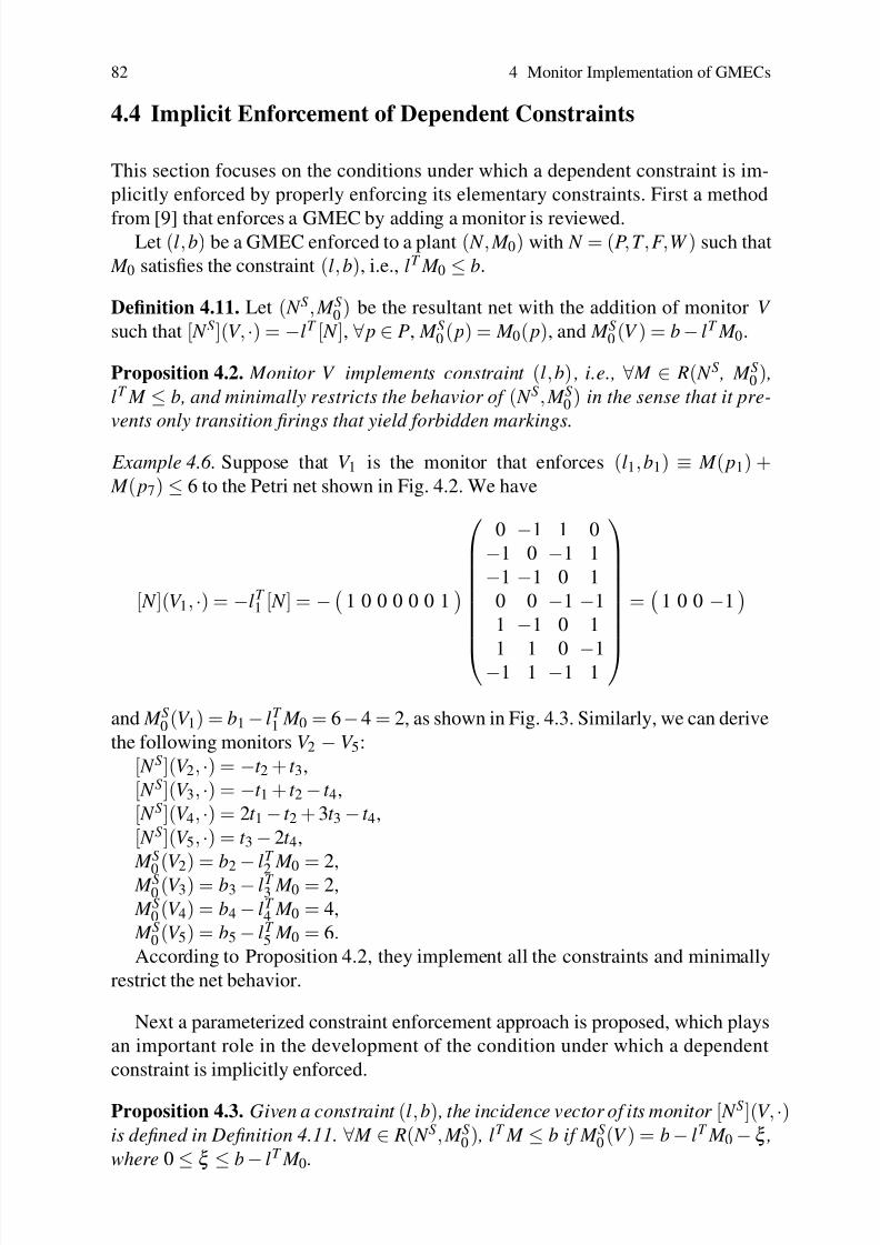
8/4/2019 Li Z., Zhou M. Deadlock Resolution in Automated Manufacturing Systems - A Novel Petri Net Approach
http://slidepdf.com/reader/full/li-z-zhou-m-deadlock-resolution-in-automated-manufacturing-systems-a-novel 97/249
82 4 Monitor Implementation of GMECs
4.4 Implicit Enforcement of Dependent Constraints
This section focuses on the conditions under which a dependent constraint is im-
plicitly enforced by properly enforcing its elementary constraints. First a method
from [9] that enforces a GMEC by adding a monitor is reviewed.Let (l,b) be a GMEC enforced to a plant ( N , M 0) with N = (P,T ,F ,W ) such that
M 0 satisfies the constraint (l,b), i.e., lT M 0 ≤ b.
Definition 4.11. Let ( N S, M S0 ) be the resultant net with the addition of monitor V
such that [ N S](V , ·) = −lT [ N ], ∀ p ∈ P, M S0 ( p) = M 0( p), and M S0 (V ) = b − lT M 0.
Proposition 4.2. Monitor V implements constraint (l,b) , i.e., ∀ M ∈ R( N S , M S0 ) ,lT M ≤ b, and minimally restricts the behavior of ( N S, M S0 ) in the sense that it pre-
vents only transition firings that yield forbidden markings.
Example 4.6. Suppose that V 1 is the monitor that enforces (l1,b1) ≡ M ( p1) + M ( p7) ≤ 6 to the Petri net shown in Fig. 4.2. We have
[ N ](V 1, ·) = −lT 1 [ N ] = − 1 0 0 0 0 0 1
⎛⎜⎜⎜⎜⎜⎜⎜⎜⎝
0 −1 1 0
−1 0 −1 1
−1 −1 0 1
0 0 −1 −1
1 −1 0 1
1 1 0 −1−1 1 −1 1
⎞⎟⎟⎟⎟⎟⎟⎟⎟⎠
=
1 0 0 −1
and M S0 (V 1) = b1 − lT 1 M 0 = 6−4 = 2, as shown in Fig. 4.3. Similarly, we can derive
the following monitors V 2 − V 5:
[ N S](V 2, ·) = −t 2 + t 3,
[ N S](V 3, ·) = −t 1 + t 2 − t 4,
[ N S](V 4, ·) = 2t 1 − t 2 + 3t 3 − t 4,
[ N S](V 5, ·) = t 3 − 2t 4,
M S
0(V 2) = b2
−lT
2M 0 = 2,
M S0 (V 3) = b3 − lT 3 M 0 = 2,
M S0 (V 4) = b4 − lT 4 M 0 = 4,
M S0 (V 5) = b5 − lT 5 M 0 = 6.
According to Proposition 4.2, they implement all the constraints and minimally
restrict the net behavior.
Next a parameterized constraint enforcement approach is proposed, which plays
an important role in the development of the condition under which a dependent
constraint is implicitly enforced.
Proposition 4.3. Given a constraint (l,b) , the incidence vector of its monitor [ N S](V , ·)is defined in Definition 4.11. ∀ M ∈ R( N S, M S0 ) , lT M ≤ b if M S0 (V ) = b − lT M 0 −ξ ,
where 0 ≤ ξ ≤ b − lT M 0.

8/4/2019 Li Z., Zhou M. Deadlock Resolution in Automated Manufacturing Systems - A Novel Petri Net Approach
http://slidepdf.com/reader/full/li-z-zhou-m-deadlock-resolution-in-automated-manufacturing-systems-a-novel 98/249
4.4 Implicit Enforcement of Dependent Constraints 83
p 1
p 5
p 4
t 3
t 2
t 1
t 4
p 6 p 7
p 3
p 2
V 1
t 1 t 4
t 3
t 2
V 2
V 3t 1
t 2 t 4
V 4
V 5
t 2t 3
t 1
t 4
t 3 t 4
6
4
2
3
2
Fig. 4.3 A controlled system ( N S, M S0 )
Proof. Since 0
≤ξ
≤b
−lT M 0,
∀ M
∈ R( N , M 0), lT M
≤b
−ξ
≤b. That is to say,
any reachable marking in ( N S, M S0 ) satisfies the constraint (l,b). ⊓⊔Similarly to the control depth variable of a siphon in [34], ξ is called the control
depth variable of a constraint (l,b). For (l1,b1) ≡ M ( p1) + M ( p7) ≤ 6 in Fig. 4.2,
ξ1 = 1 means that M S0 (V 1) = 1.
Let (l,b) be a GMEC to ( N , M 0). We define
M lmax = maxlT M | M ∈ R( N , M 0) (4.1)
and
M lmin = minlT M | M ∈ R( N , M 0). (4.2)
Example 4.7. The Petri net shown in Fig. 4.2 has 11 reachable states. For (l1,b1),
(l2,b2), and (l3,b3), it is easy to find that M l1max = 5, M
l1min = 3, M
l2max = 5, M
l2min = 3,
M l3max = 8, and M
l3min = 4.
Theorem 4.3. Let (l,b) be a strongly dependent constraint with η = ∑ni=1 aiηi and
l
= ∑
ni=1 aili. (l,b) is redundant with respect to ( N , M 0) if
lT M 0 −n
∑i=1
ailT i M 0 +
n
∑i=1
ai M limax ≤ b.

8/4/2019 Li Z., Zhou M. Deadlock Resolution in Automated Manufacturing Systems - A Novel Petri Net Approach
http://slidepdf.com/reader/full/li-z-zhou-m-deadlock-resolution-in-automated-manufacturing-systems-a-novel 99/249
84 4 Monitor Implementation of GMECs
Proof. Since
η =n
∑i=1
aiηi,
we have
lT [ N ] =n
∑i=1
ailT i [ N ].
It is easy to see that
(l −n
∑i=1
aili)T [ N ] = 0T .
Since l = ∑ni=1 aili, we conclude that
l −n
∑i=1
aili
is a P-invariant of N .
This implies that ∀ M ∈ R( N , M 0),
(l −n
∑i=1 aili)
T
M = (l −n
∑i=1 aili)
T
M 0. (4.3)
From (4.3), we have
lT M = lT M 0 −n
∑i=1
ailT i M 0 +
n
∑i=1
ailT i M (4.4)
and
lT M
≤lT M 0
−
n
∑i=1
ailT i M 0 +
n
∑i=1
ai M limax.
Clearly, lT M ≤ b is true if
lT M 0 −n
∑i=1
ailT i M 0 +
n
∑i=1
ai M limax ≤ b. (4.5)
⊓⊔ Example 4.8. As stated previously, (l5,b5) ≡ M ( p3) + M ( p5) + M ( p6) + M ( p7) ≤14 in Fig. 4.2 is a strongly dependent constraint with respect to (l1,b1), (l2,b2), and
(l3,b3) with η5 = η1 +η2 +η3. We have
lT 5 M 0 = M 0( p3) + M 0( p5) + M 0( p6) + M 0( p7) = 8,
lT 1 M 0 = M 0( p1) + M 0( p7) = 4,
lT 2 M 0 = M 0( p2) + M 0( p6) = 4,

8/4/2019 Li Z., Zhou M. Deadlock Resolution in Automated Manufacturing Systems - A Novel Petri Net Approach
http://slidepdf.com/reader/full/li-z-zhou-m-deadlock-resolution-in-automated-manufacturing-systems-a-novel 100/249
4.4 Implicit Enforcement of Dependent Constraints 85
lT 3 M 0 = M 0( p3) + M 0( p5) + M 0( p6) = 5,
M l1max = 5,
M l2max = 5,
M l3max = 8.
Considering b5 = 14, we have lT 5 M 0 −∑
3i=1 ail
T i M 0 +∑
3i=1 ai M
li
max < b5. As aresult, (l5,b5) ≡ M ( p3) + M ( p5) + M ( p6) + M ( p7) ≤ 14 is redundant with respect
to the Petri net in Fig. 4.2.
Theorem 4.4. Let (l,b) be a strongly dependent constraint with η = ∑ni=1 aiηi and
l = ∑ni=1 aili in a Petri net ( N , M 0). (l,b) is redundant with respect to ( N , M 0) if
n
∑i=1
aibi ≤ b.
Proof. ∀ M ∈ R( N , M 0), we have lT M = ∑ni=1 ail
T i M ≤ ∑
ni=1 aibi ≤ b. This result is
true. ⊓⊔ Example 4.9. Suppose that there is a set of GMECs (l1,b1) ≡ M ( p2) ≤ 2, (l2,b2) ≡ M ( p3) ≤ 1, and (l3,b3) ≡ 2 M ( p2) + M ( p3) ≤ 10 for the Petri net shown in Fig.
4.4(a). Their corresponding monitors are shown in Fig. 4.4(b). The fact l3 = 2l1 + l2
can be verified. Clearly, we have 2b1 + b2 < b3 and thus conclude that (l3,b3) is
redundant.
p 1
p 2
t 2
t 1
p 3
t 3
5
( b )
1 0
2
V 1
V 3
V 2
p 1
p 2
t 2
t 1
p 3
t 3
5
( a )
Fig. 4.4 (a) a plant ( N , M 0) and (b) the controlled system ( N S, M S0 )
Theorem 4.5. Let (l,b) be a weakly dependent GMEC withη =∑ni=1 aiηi −∑m
j=1 a jη j
and l
= ∑
n
i=1
aili
−∑
m
j=1
a jl j in a plant ( N , M 0). It is redundant with respect to
( N , M 0) if
lT M 0 −n
∑i=1
ailT i M 0 +
m
∑ j=1
a jlT j M 0 +
n
∑i=1
ai M limax −
m
∑ j=1
a j M l j
min ≤ b.

8/4/2019 Li Z., Zhou M. Deadlock Resolution in Automated Manufacturing Systems - A Novel Petri Net Approach
http://slidepdf.com/reader/full/li-z-zhou-m-deadlock-resolution-in-automated-manufacturing-systems-a-novel 101/249
86 4 Monitor Implementation of GMECs
Proof. Since
η =n
∑i=1
aiηi −m
∑ j=1
a jη j (4.6)
we have
(l −n
∑i=1
aili +m
∑ j=1
a jl j)T [ N ] = 0T , (4.7)
indicating that
l −n
∑i=1
aili +m
∑ j=1
a jl j
is a P-invariant of N .
As a result, ∀ M ∈ R( N , M 0),
lT M 0 −n
∑i=1
ailT i M 0 +
m
∑ j=1
a jlT j M 0 = lT M −
n
∑i=1
ailT i M +
m
∑ j=1
a jlT j M ,
i.e.,
l
T
M = l
T
M 0 −n
∑i=1 ail
T
i M 0 +
m
∑ j=1 a jl
T
j M 0 +
n
∑i=1 ail
T
i M −m
∑ j=1 a jl
T
j M .
It is easy to see that
lT M ≤ lT M 0 −n
∑i=1
ailT i M 0 +
m
∑ j=1
a jlT j M 0 +
n
∑i=1
ai M limax −
m
∑ j=1
a j M l j
min.
Hence, lT M ≤ b can be obtained from
lT M 0 −n
∑i=1
ailT i M 0 +
m
∑ j=1
a jlT j M 0 +
n
∑i=1
ai M limax −
m
∑ j=1
a j M l jmin ≤ b.
⊓⊔
Theorem 4.6. Let (l,b) be a weakly dependent GMEC with η = ∑ni=1 aiηi− ∑
m j=1
a jη j and l = ∑ni=1 aili −∑m
j=1 a jl j. It is redundant with respect to ( N , M 0) if
n
∑i=1
aibi
−
m
∑ j=1
a jb j
≤b.

8/4/2019 Li Z., Zhou M. Deadlock Resolution in Automated Manufacturing Systems - A Novel Petri Net Approach
http://slidepdf.com/reader/full/li-z-zhou-m-deadlock-resolution-in-automated-manufacturing-systems-a-novel 102/249
4.4 Implicit Enforcement of Dependent Constraints 87
Proof. Similar to the proof of Theorem 4.4. ⊓⊔Note that in [9], the redundancy of a GMEC such as (l3,b3) ≡ 2 M ( p2)+ M ( p3) ≤
10 in Example 4.9 can be verified by solving an LPP, as stated in Proposition 4.1.
It is clear that the computational complexity of Theorem 4.3 to decide the redun-
dancy of a dependent constraint is worse than Proposition 4.1 since the complete
state enumeration is needed in Theorem 4.3. However, it is shown next that the re-
dundancy of all dependent GMECs can be determined by solving 2 | L E | LPPs only,
where | L E | ≤ min|P|, |T |.
Let (l,b) be a GMEC in a Petri net ( N , M 0). We define
M l MAX = maxlT M | M = M 0 + [ N ]Y , M ≥ 0,Y ≥ 0 (4.8)
and
M l MIN = minlT M | M = M 0 + [ N ]Y , M ≥ 0,Y ≥ 0. (4.9)
Clearly, we have
M l MAX ≥ M lmax (4.10)
and
M l MIN ≤ M lmin (4.11)
It is trivial that (4.8) and (4.9) can be found in polynomial time by solving LPPs.In Fig. 4.2, it is easy to find that M
l1 MAX = 5, M
l2 MAX = 5, M
l3 MAX = 8, M
l1 MIN = 3,
M l2
MIN = 3, and M l3
MIN = 4.
Corollary 4.1. Let (l,b) be a strongly dependent constraint with η = ∑ni=1 aiηi and
l = ∑ni=1 aili in ( N , M 0). (l,b) is redundant with respect to ( N , M 0) if
lT M 0 −n
∑i=1
ailT i M 0 +
n
∑i=1
ai M li
MAX ≤ b.
Proof. It follows immediately from Theorem 4.3 and (4.10). ⊓⊔Corollary 4.2. Let (l,b) be a weakly dependent GMEC in Petri net ( N , M 0) with
η =∑ni=1 aiηi −∑m
j=1 a jη j and l =∑ni=1 aili −∑m
j=1 a jl j. It is redundant with respect
to ( N , M 0) if
lT M 0 −n
∑i=1
ailT i M 0 +
m
∑ j=1
a jlT j M 0 +
n
∑i=1
ai M li
MAX −m
∑ j=1
a j M l j
MIN ≤ b.
Corollaries 4.1 and 4.2 indicate that the redundancy of (weakly and strongly)
dependent constraints can be decided provided that M li
MAX and M li
MIN are known,

8/4/2019 Li Z., Zhou M. Deadlock Resolution in Automated Manufacturing Systems - A Novel Petri Net Approach
http://slidepdf.com/reader/full/li-z-zhou-m-deadlock-resolution-in-automated-manufacturing-systems-a-novel 103/249
88 4 Monitor Implementation of GMECs
where i ∈ N| L E |. That is to say, due to the two corollaries, the redundancy of de-
pendent constraints can be decided by solving 2| L E | LPPs no matter how many
dependent constraints in a set of GMECs. However, as stated in Proposition 4.1, the
verification of the redundancy of each GMEC needs to solve an LPP.
A parameterized approach is next presented for a dependent constraint (l,b) withη = ∑ni=1 aiηi that can be implicitly enforced to a plant ( N , M 0) by properly setting
the control depth variables of its elementary constraints. The implicit enforcement
of (l,b) implies that it is redundant with respect to the augmented net with additional
monitors ( N S, M S0 ).
Theorem 4.7. Let (l,b) be a strongly dependent constraint of Petri net ( N , M 0) with
η = ∑ni=1 aiηi and l = ∑
ni=1 aili. ∀i ∈ Nn , (li,bi) is enforced by adding a monitor
V i with its control depth variable ξi , as stated in Proposition 4.3. Then, (l,b) is
implicitly enforced to ( N , M 0) if
n
∑i=1
aiξi ≥ (lT M 0 − b) +n
∑i=1
ai(bi − lT i M 0).
Proof. According to Theorem 4.3, (l,b) is implicitly enforced if
lT M 0 −n
∑i=1
ailT i M 0 +
n
∑i=1
ai M limax ≤ b.
By Proposition 4.3, ∀i ∈ Nn, if a monitor V i is added such that (li,bi) is enforcedwith M S0 (V i) = bi − lT
i M 0 −ξi, we have M limax = bi −ξi. As a result, (l,b) is implicitly
enforced if
lT M 0 −n
∑i=1
ailT i M 0 +
n
∑i=1
ai(bi −ξi) ≤ b,
i.e.,
n
∑i=1 aiξi ≥ (l
T
M 0 − b) +
n
∑i=1 ai(bi − l
T
i M 0).
⊓⊔ Example 4.10. Suppose that (l5,b5) ≡ M ( p3) + M ( p5) + M ( p6) + M ( p7) ≤ 9 is a
GMEC in Fig. 4.2. As is known, η5 = η1 +η2 +η3. It is not redundant with respect
to its elementary constraints (l1,b1), (l2,b2), and (l3,b3). However, it can be made
redundant if setting the control depth variables by ∑3i=1 ξi ≥ (lT
5 M 0 − b5) + (b1 −lT
1 M 0)+(b2 − lT 2 M 0)+(b3 − lT
3 M 0), where b5 = 9, lT 5 M 0 = 8, b1 = 6, b2 = 6, b3 = 7,
lT
1M
0= 4, lT
2M
0= 4, and lT
3M
0= 5. That is to say, (l
5,b
5)≡
M ( p3
) + M ( p5
) + M ( p6) + M ( p7) ≤ 9 is redundant if ∑
3i=1 ξi ≥ (8−9) + (6−4) + (6−4) + (7−5) =
5. Specifically, let ξ1 = ξ2 = 2 and ξ3 = 1. (l5,b5) ≡ M ( p3) + M ( p5) + M ( p6) + M ( p7) ≤ 9 is redundant if (l1,b1), (l2,b2), and (l3,b3) are enforced by monitors V 1,

8/4/2019 Li Z., Zhou M. Deadlock Resolution in Automated Manufacturing Systems - A Novel Petri Net Approach
http://slidepdf.com/reader/full/li-z-zhou-m-deadlock-resolution-in-automated-manufacturing-systems-a-novel 104/249
4.4 Implicit Enforcement of Dependent Constraints 89
V 2, and V 3 with M S0 (V 1) = b1 −ξ1 − lT 1 M 0 = 0, M S0 (V 2) = b2 −ξ2 − lT
2 M 0 = 0, and
M S0 (V 3) = b3 −ξ3 − lT 3 M 0 = 1.
Theorem 4.8. Let (l,b) be a strongly dependent constraint of Petri net ( N , M 0) with
η = ∑ni=1 aiηi and l = ∑
ni=1 aili , where ηi = [ N ]T li.
∀i
∈Nn , (li,bi) is enforced by
adding a monitor V i with its control depth variable ξi , as stated in Proposition 4.3.
(l,b) is implicitly enforced if
n
∑i=1
ai(bi −ξi) ≤ b.
Proof. It follows from Theorem 4.4 and Proposition 4.3. ⊓⊔Theorem 4.9. Let (l,b) be a weakly dependent constraint in a Petri net ( N , M 0) with
η=∑
n
i=1a
iη
i −∑
m
j=1a
jη
jand l
=∑
n
i=1a
il
i −∑
m
j=1a
jl j
.∀
i∈Nn
,(
li,
bi)
is enforced
by adding a monitor V i with control depth variable ξi according to Proposition 4.3.
(l,b) is implicitly enforced to ( N , M 0) if
n
∑i=1
aiξi ≥ (lT M 0 − b) +n
∑i=1
ai(bi − lT i M 0) +
m
∑ j=1
a jlT j M 0.
Proof. Due to Theorem 4.5, (l,b) is implicitly enforced if
lT M 0 −n
∑i=1
ailT i M 0 +
m
∑ j=1
a jlT j M 0 +
n
∑i=1
ai M limax −
m
∑ j=1
a j M l j
min ≤ b. (4.12)
From Proposition 4.3, we have M limax = bi −ξi and M
l j
min ≥ 0. As a result,
lT M 0 −n
∑i=1
ailT i M 0 +
m
∑ j=1
a jlT j M 0 +
n
∑i=1
ai(bi −ξi) ≤ b (4.13)
implies the truth of (4.12).
From (4.13), we haven
∑i=1
aiξi ≥ (lT M 0 − b) +n
∑i=1
ai(bi − lT i M 0) +
m
∑ j=1
a jlT j M 0.
⊓⊔Theorem 4.10. Let (l,b) be a weakly dependent constraint to a Petri net ( N , M 0)with η = ∑
ni=1 aiηi −∑m
j=1 a jη j and l = ∑ni=1 aili −∑m
j=1 a jl j . ∀i ∈ Nn , (li,bi) is
enforced by adding a monitor V i with control depth variable ξi according to Propo-
sition 4.3. It is implicitly enforced to ( N , M 0) if
n
∑i=1
ai(bi −ξi) −m
∑ j=1
a jb j ≤ b.

8/4/2019 Li Z., Zhou M. Deadlock Resolution in Automated Manufacturing Systems - A Novel Petri Net Approach
http://slidepdf.com/reader/full/li-z-zhou-m-deadlock-resolution-in-automated-manufacturing-systems-a-novel 105/249
90 4 Monitor Implementation of GMECs
4.5 Application to Deadlock Prevention
This section presents the application of the methods presented in this chapter to a
deadlock prevention policy developed by Park and Reveliotis in [40]. It is shown
that these methods may reduce the structural complexity of the liveness-enforcingsupervisor for a class of Petri nets, S3PGR2. It stands for system of simple sequential
processes with general resource requirements. As stated in Chap. 1, an S3PGR2 is
equivalent to an S4R. For simplicity, we use S4R to denote the class of Petri nets in
the rest of this book.
Definition 4.12. A well-marked S4R net is a marked Petri net N = (P,T ,F ,W ) with
initial marking M 0 such that:
1. P = P A
∪P0
∪P R, where P A =
∪n j=1P A j
is called the set of operation places such
that P Ai∩ P A j
= / 0, ∀i = j, P0 = ∪ni=1 p0
i is called the set of idle places with
P0 ∩ P A = / 0, and P R = r 1,r 2, · · · ,r m is called the set of resource places such
that (P0 ∪ P A)∩ P R = / 0.
2. T = ∪n j=1T j, and ∀i = j, T i ∩ T j = / 0.
3. W = W A ∪W R, where W A : ((P A ∪ P0) × T ) ∪ (T × (P A ∪ P0)) → 0,1 such that
∀ j = i, ((P A j∪ p0
j)×T i)∪(T i ×(P A j∪ p0
j)) → 0, and W R : (P R ×T )∪(T ×P R) → N.
4. ∀ j ∈Nn, the subnet N j derived from P A j∪ p0
j∪T j is a strongly connected state
machine such that every circuit contains p0
j .5. ∀r ∈ P R, there exists a unique P-semiflow I r such that || I r ||∩P R = r , || I r ||∩P0 =
/ 0, || I r || ∩ P A = / 0, and I r (r ) = 1. Furthermore, P A = (∪r ∈P R|| I r ||) \ P R.
6. N is pure and strongly connected.
7. ∀ p ∈ P A, M 0( p) = 0; ∀r ∈ P R, M 0(r ) ≥ max p∈|| I r || I r ( p); and ∀ p0 j ∈ P0, M 0( p0
j ) ≥1.
From its definition, an S4R is equivalent to an S4PR. The following result about
the rank of the incidence matrix of an S4R is from [43].
Theorem 4.11. Let N = (P A ∪ P0 ∪ P R,T ,F ,W ) be an S4 R. Then, rank ([ N ]) = |P A|.For an S4R, Park and Reveliotis [40] develop a deadlock prevention policy that is
of polynomial complexity. The liveness requirements in an S4R are represented by
a set of GMECs that can be implemented by a set of monitors. The policy considers
a system that is formally defined by a set of resources R = r i|i ∈ Nm and a set
of jobs J = J j| j ∈ Nn. Each resource type r i has a capacity C i ∈ N+. Each job
type J j is defined by a set of operations p jk |k ∈ Nλ j ,λ j ∈ N+, which is partially
ordered through a set of precedence constraints. Each job operation p jk is associated
with a conjunctive resource allocation requirement, formally expressed by an m-dimensional vector a p jk
, with a p jk [i], i ∈Nm, indicating how many units of resource
r i are required to support the operation execution. Such a system can be modeled by
a class of Petri nets, namely S4R, that is more general than S3PR [8]. Let ( N , M 0)

8/4/2019 Li Z., Zhou M. Deadlock Resolution in Automated Manufacturing Systems - A Novel Petri Net Approach
http://slidepdf.com/reader/full/li-z-zhou-m-deadlock-resolution-in-automated-manufacturing-systems-a-novel 106/249
4.5 Application to Deadlock Prevention 91
denote an S4R, where N = (P0 ∪ P A ∪ P R,T ,F ,W ) and P0 (P A; P R) is the set of idle
(operation; resource) places.
Let P0 = p10, p11, P A = p1, p2, p3, p4, p5, p6, and P R = r 1, r 2, r 3. The
Petri net shown in Fig. 4.5 is an S4R that is the model of an FMS that can produce
two job types J 1 and J 2 with J 1 = p1, p2, p3 and J 2 = p4, p5, p6. There arethree resources r 1, r 2, and r 3 in the system. Furthermore, we have C 1 = 3, C 2 = 2,
and C 3 = 1. An operation place that has no subsequent processing stage is called a
terminal operation. For example, p3 and p6 are terminal operation places.
p 1
p 3
p 6
p 4
p 5p 2
r1
p 1 1
p 1 0
r3
r2
t 1t 8
t 7
t 6
t 5t 4
t 3
t 2 3
2
2
2
Fig. 4.5 An S4R ( N , M 0)
Note that each resource place r corresponds to a minimal P-semiflow I r . As a
result, we have three minimal P-semiflows that are associated with resources. They
are
I r 1 = r 1 + p1 + 3 p2 + p6,
I r 2 = r 2 + p2 + 2 p5 + 2 p6, I r 3 = r 3 + p3 + p4.
A minimal P-semiflow I r associated with the resource place r shows the opera-
tion places whose execution requires resource r and how many units of resource r
are needed to support the operation execution. Hence, the conjunctive resource re-
quirements of operations can be easily obtained as follows: a p1= (1,0,0)T , a p2
=(3,1,0)T , a p3
= (0,0,1)T , a p4= (0,0,1)T , a p5
= (0,2,0)T , and a p6= (1,2,0)T .
Let oi ≡ O(r i), O : R → Nm be any partial order imposed on the resource set R.
Given p ∈ P A, let ρmax p = maxoi|a p[i] > 0, i ∈Nm and ρmin
p = minoi|a p[i] > 0, i ∈
Nm. Also, let L
p = q|q
∈ ( p
•)• ∩P
A ∧ρmax
q =min
v∈( p•)•∩P Aρ
max
v . By convention,
L p = / 0 if ( p•)• ∩ P0 = / 0. Then:
1. The neighborhood set N p of p ∈ P A is defined by N p = p∪q|q ∈ ∪v∈ L p N v ∧ρmin
p ≤ ρmaxq .

8/4/2019 Li Z., Zhou M. Deadlock Resolution in Automated Manufacturing Systems - A Novel Petri Net Approach
http://slidepdf.com/reader/full/li-z-zhou-m-deadlock-resolution-in-automated-manufacturing-systems-a-novel 107/249
92 4 Monitor Implementation of GMECs
2. The adjusted resource allocation requirement a p for p ∈ P A under partial order
O() (resource ordering) is given by a p[i] = maxaq[i]|q ∈ N p if oi ≥ ρmin p ; oth-
erwise a p[i] = 0, ∀i ∈ Nm.
3. The policy-imposed constraint on the system operation is expressed by the re-
quirement that no resource is over-allocated with respect to the adjusted opera-tion requirements specified by a p[i].
Consider the net shown in Fig. 4.5 under the resource order o1 = 2, o2 = 3, and
o3 = 1. Note that different resource orderings may lead to different sets of GMECs
[39]. The neighborhood sets associated with the operation places p ∈ P A can be
computed starting from the terminal operation places in the partially ordered sets
that correspond to the job types in the system, and proceeding backward. For job
type J1, we have
• ρmax
p3 = 1, ρmin
p3 = 1, L p3 = / 0 by ( p•3)• ∩ P0
= / 0, and N p3 = p3;• ρmax p2
= 3, ρmin p2
= 2, L p2= p3, N p2
= p2;
• ρmax p1
= 2, ρmin p1
= 2, L p1= p2, and N p1
= p1, p2.
For job type J2, we have
• ρmax p6
= 3, ρmin p6
= 2, L p6= / 0 by ( p•
6)• ∩ P0 = / 0, and N p6= p6;
• ρmax p5
= 3, ρmin p5
= 3, L p5= p6, and N p5
= p5, p6;
• ρmax p4
= 1, ρmin p4
= 1, L p4= p5, and N p4
= p4, p5, p6.
The adjusted resource allocation requirements can be found as follows:
a p1=
⎛⎝ 3
1
0
⎞⎠, a p2
=
⎛⎝ 3
1
0
⎞⎠, a p3
=
⎛⎝ 0
0
1
⎞⎠, a p4
=
⎛⎝1
2
1
⎞⎠, a p5
=
⎛⎝ 0
2
0
⎞⎠, a p6
=
⎛⎝ 1
2
0
⎞⎠.
By imposing on the operation places a set of linear inequality constraints that are
implemented by monitors, the supervised system has no deadlock states, implying
that liveness is ensured. The set of inequality constraints takes the form of
ˆ A p · M P ≤ f p (4.14)
where the column vector in ˆ A p corresponding to an operation place p is a p, vector
M P is the restriction of marking M to operation places, and f p is the capacity vector
of resources, i.e., f p(i) = C i, i ∈ N| R|.For the net shown in Fig. 4.5, we have
⎛⎝ 3 3 0 1 0 1
1 1 0 2 2 20 0 1 1 0 0
⎞⎠ ·
⎛
⎜⎜⎜⎜⎜⎜⎝
M ( p1) M ( p2)
M ( p3) M ( p4) M ( p5) M ( p6)
⎞
⎟⎟⎟⎟⎟⎟⎠≤⎛⎝ 3
21
⎞⎠ .

8/4/2019 Li Z., Zhou M. Deadlock Resolution in Automated Manufacturing Systems - A Novel Petri Net Approach
http://slidepdf.com/reader/full/li-z-zhou-m-deadlock-resolution-in-automated-manufacturing-systems-a-novel 108/249
4.5 Application to Deadlock Prevention 93
By extending ˆ A p and M P, the liveness control requirements stated in (4.14) can
be described as
ˆ A · M ≤ f p (4.15)
where ˆ A is derived from ˆ A p by adding zero column vectors that correspond to idleand resource places and M is any marking in R( N , M 0). It is easy to see that (4.15)
is a typical set of GMECs ( ˆ A, f p).
For the net in Fig. 4.5, its liveness requirement represented by ˆ A · M ≤ f p takes
the following specific form, where we assume that the places are ordered in the
incidence matrix according to the sequence p1, p2, p3, p4, p5, p6, p10, p11, r 1, r 2,
r 3. Figure 4.6 shows the controlled system of the S4R in Fig. 4.5.
⎛⎝ 3 3 0 1 0 1 0 0 0 0 0
1 1 0 2 2 2 0 0 0 0 0
0 0 1 1 0 0 0 0 0 0 0
⎞⎠ ·
⎛⎜⎜⎜⎜⎜⎜⎜⎜⎜⎜⎜⎜⎜⎜⎜⎜⎝
M ( p1)
M ( p2) M ( p3) M ( p4) M ( p5) M ( p6)
M ( p10) M ( p11) M (r 1) M (r 2)
M (r 3)
⎞⎟⎟⎟⎟⎟⎟⎟⎟⎟⎟⎟⎟⎟⎟⎟⎟⎠
≤⎛⎝ 3
2
1
⎞⎠ .
If we can distinguish redundant constraints imposed on the plant, a structurally
simple liveness-enforcing supervisor may be found. To demonstrate this, a flexi-
ble manufacturing example is investigated. Its liveness-enforcing supervisor is first
computed by the deadlock prevention policy in [40]. Then, we show how a simpler
supervisor is synthesized.
Example 4.11. Figure 4.7 is the Petri net model of an FMS. It consists of nine re-
source places R1−R9, two idle places p1 and p6, and seven operation places p2− p5
and p7− p9. The Petri net is an S
4
R that contains two processes with operation setsP1 = p2, p3, p4, p5 and P2 = p7, p8, p9. The resource capacity vector is f p = (1
1 1 3 4 1 3 3 2)T . The conjunctive resource requirements of operations are
a p2=
⎛⎜⎜⎜⎜⎜⎜⎜⎜⎜⎜⎜⎜⎝
1
0
0
0
1
0
0
0
0
⎞⎟⎟⎟⎟⎟⎟⎟⎟⎟⎟⎟⎟⎠
, a p3=
⎛⎜⎜⎜⎜⎜⎜⎜⎜⎜⎜⎜⎜⎝
0
1
0
0
1
0
1
0
0
⎞⎟⎟⎟⎟⎟⎟⎟⎟⎟⎟⎟⎟⎠
, a p4=
⎛⎜⎜⎜⎜⎜⎜⎜⎜⎜⎜⎜⎜⎝
0
0
0
1
0
1
1
0
0
⎞⎟⎟⎟⎟⎟⎟⎟⎟⎟⎟⎟⎟⎠
, a p5=
⎛⎜⎜⎜⎜⎜⎜⎜⎜⎜⎜⎜⎜⎝
0
0
1
0
0
0
1
0
0
⎞⎟⎟⎟⎟⎟⎟⎟⎟⎟⎟⎟⎟⎠
,

8/4/2019 Li Z., Zhou M. Deadlock Resolution in Automated Manufacturing Systems - A Novel Petri Net Approach
http://slidepdf.com/reader/full/li-z-zhou-m-deadlock-resolution-in-automated-manufacturing-systems-a-novel 109/249
94 4 Monitor Implementation of GMECs
p 1
p 3
p 6
p 4
p 5p 2
r1
p 1 1
p 1 0
r3
r2
t 1 t 8
t 7
t 6
t 5t 4
t 3
t 2 3
2
2
2
V 1t 1
t 3
t 8
t 7
t 6
t 53
3
V 2t 1 t 8
t 5t 3
2
2
t 3
t 4 t 5
t 6V 3
Fig. 4.6 The controlled system of the S4R in Fig. 4.5
a p7
=
⎛⎜⎜⎜⎜⎜⎜⎜⎜⎜⎜⎜⎜⎝
0
0
1
1
0
0
0
0
1
⎞⎟⎟⎟⎟⎟⎟⎟⎟⎟⎟⎟⎟⎠
, a p8
=
⎛⎜⎜⎜⎜⎜⎜⎜⎜⎜⎜⎜⎜⎝
0
1
0
0
0
0
0
1
1
⎞⎟⎟⎟⎟⎟⎟⎟⎟⎟⎟⎟⎟⎠
, a p9
=
⎛⎜⎜⎜⎜⎜⎜⎜⎜⎜⎜⎜⎜⎝
1
0
0
0
0
0
0
1
0
⎞⎟⎟⎟⎟⎟⎟⎟⎟⎟⎟⎟⎟⎠
.
Under the resource order o1 = 1, o2 = 1, o3 = 1, o4 = 3, o5 = 4, o6 = 1, o7 = 3,
o8 = 3, and o9 = 3, we have
a p2=
⎛⎜⎜⎜⎜⎜⎜⎜⎜⎜⎜⎜⎜⎝
1
11
1
1
1
1
0
0
⎞⎟⎟⎟⎟⎟⎟⎟⎟⎟⎟⎟⎟⎠
, a p3=
⎛⎜⎜⎜⎜⎜⎜⎜⎜⎜⎜⎜⎜⎝
0
11
1
1
1
1
0
0
⎞⎟⎟⎟⎟⎟⎟⎟⎟⎟⎟⎟⎟⎠
, a p4=
⎛⎜⎜⎜⎜⎜⎜⎜⎜⎜⎜⎜⎜⎝
0
00
1
0
1
1
0
0
⎞⎟⎟⎟⎟⎟⎟⎟⎟⎟⎟⎟⎟⎠
, a p5=
⎛⎜⎜⎜⎜⎜⎜⎜⎜⎜⎜⎜⎜⎝
0
01
0
0
0
1
0
0
⎞⎟⎟⎟⎟⎟⎟⎟⎟⎟⎟⎟⎟⎠
,

8/4/2019 Li Z., Zhou M. Deadlock Resolution in Automated Manufacturing Systems - A Novel Petri Net Approach
http://slidepdf.com/reader/full/li-z-zhou-m-deadlock-resolution-in-automated-manufacturing-systems-a-novel 110/249
4.5 Application to Deadlock Prevention 95
a p7 =
⎛⎜⎜⎜⎜⎜⎜⎜⎜⎜⎜⎜⎜⎝
1
1
1
1
0
0
0
1
1
⎞⎟⎟⎟⎟⎟⎟⎟⎟⎟⎟⎟⎟⎠,
a p8 =
⎛⎜⎜⎜⎜⎜⎜⎜⎜⎜⎜⎜⎜⎝
1
1
0
0
0
0
0
1
1
⎞⎟⎟⎟⎟⎟⎟⎟⎟⎟⎟⎟⎟⎠,
a p9 =
⎛⎜⎜⎜⎜⎜⎜⎜⎜⎜⎜⎜⎜⎝
1
0
0
0
0
0
0
1
0
⎞⎟⎟⎟⎟⎟⎟⎟⎟⎟⎟⎟⎟⎠.
t 1
t 2
t 3
t 4
t 5
t 6
p 1
p 2
p 3
p 4p 5
R 5
R 6
t 1 0
t 9
p 9
p 8
t 8
p 7
t 7
p 6
R 8
R 9
R 1
R 2
R 3
R 4
R 7
45
4
Fig. 4.7 The Petri net model ( N , M 0) of an FMS
From ˆ A p = [a p2 |a p3 |a p4 |a p5 |a p7 |a p8 |a p9 ], the liveness control specifications arerepresented by a set of GMECs, i.e., ˆ A · M ≤ f p, or,
⎛⎜⎜⎜⎜⎜⎜⎜⎜⎜⎜⎜⎜⎝
0 1 0 0 0 0 1 1 1 0 0 0 0 0 0 0 0 0
0 1 1 0 0 0 1 1 0 0 0 0 0 0 0 0 0 0
0 1 1 0 1 0 1 0 0 0 0 0 0 0 0 0 0 0
0 1 1 1 0 0 1 0 0 0 0 0 0 0 0 0 0 0
0 1 1 0 0 0 0 0 0 0 0 0 0 0 0 0 0 0
0 1 1 1 0 0 0 0 0 0 0 0 0 0 0 0 0 0
0 1 1 1 1 0 0 0 0 0 0 0 0 0 0 0 0 00 0 0 0 0 0 1 1 1 0 0 0 0 0 0 0 0 0
0 0 0 0 0 0 1 1 0 0 0 0 0 0 0 0 0 0
⎞⎟⎟⎟⎟⎟⎟⎟⎟⎟⎟⎟⎟⎠
· M ≤
⎛⎜⎜⎜⎜⎜⎜⎜⎜⎜⎜⎜⎜⎝
1
1
1
3
4
1
33
2
⎞⎟⎟⎟⎟⎟⎟⎟⎟⎟⎟⎟⎟⎠
.

8/4/2019 Li Z., Zhou M. Deadlock Resolution in Automated Manufacturing Systems - A Novel Petri Net Approach
http://slidepdf.com/reader/full/li-z-zhou-m-deadlock-resolution-in-automated-manufacturing-systems-a-novel 111/249
96 4 Monitor Implementation of GMECs
The monitors that implement the above set of GMECs are shown in Table 4.1.
For each resource, a monitor is added, i.e., there are a total of nine monitors due to
the deadlock prevention policy in [40] for the Petri net model.
Table 4.1 Monitors added using the policy in [40]
V S M S0 (·) Preset Postset V S M S0 (·) Preset Postset
V 1 1 t 2,t 10 t 1, t 7 V 2 1 t 3, t 5, t 9 t 1, t 7V 3 1 t 3,t 6,t 8 t 1, t 7 V 4 3 t 4, t 5, t 8 t 1, t 7V 5 4 t 3,t 5 t 1 V 6 1 t 4, t 5 t 1V 7 3 t 4,t 6 t 1 V 8 3 t 10 t 7V 9 2 t 9 t 7
Notice that there are seven operation places. According to Theorem 4.11, the
rank of the incidence matrix of the Petri net model is seven. As a result, there are at
most seven elementary constraints in the set of GMECs. To facilitate the discussion,
the set of GMECs is rewritten as follows:
(l1,b1) ≡ M ( p2) + M ( p7) + M ( p8) + M ( p9) ≤ 1,
(l2,b2) ≡ M ( p2) + M ( p3) + M ( p7) + M ( p8) ≤ 1,
(l3,b3) ≡ M ( p2) + M ( p3) + M ( p5) + M ( p7) ≤ 1,
(l4,b4) ≡ M ( p2) + M ( p3) + M ( p4) + M ( p7) ≤ 3,
(l5,b5) ≡ M ( p2) + M ( p3) ≤ 4,
(l6,b6)
≡ M ( p2) + M ( p3) + M ( p4)
≤1,
(l7,b7) ≡ M ( p2) + M ( p3) + M ( p4) + M ( p5) ≤ 3,(l8,b8) ≡ M ( p7) + M ( p8) + M ( p9) ≤ 3,
(l9,b9) ≡ M ( p7) + M ( p8) ≤ 2.
Accordingly, we have
[η ] =
⎛⎜⎜⎜⎜⎜⎜⎜⎜⎜⎜⎜⎜⎝
1 −1 0 0 0 0 1 0 0 −1
1 0 −1 0 −1 0 1 0 −1 0
1 0 −1 0 0 −1 1 −1 0 0
1 0 0 −1 −1 0 1 −1 0 0
1 0 −1 0 −1 0 0 0 0 01 0 0 −1 −1 0 0 0 0 0
1 0 0 −1 0 −1 0 0 0 0
0 0 0 0 0 0 1 0 0 −1
0 0 0 0 0 0 1 0 −1 0
⎞⎟⎟⎟⎟⎟⎟⎟⎟⎟⎟⎟⎟⎠.
The rank of [η] is seven, implying that there are seven elementary and two de-
pendent constraints. Let L E = (l1,b1), (l2,b2), (l3,b3), (l4,b4), (l6,b6), (l8,b8),
(l9,b9). We have η5 = η2 −η9, and η7 = −η2 +η3 −η4 + 2η6 +η9. Next we
check the redundancy of the dependent constraints.
By solving LPP, we have
M l1
MAX = 3,
M l2
MAX = 3,
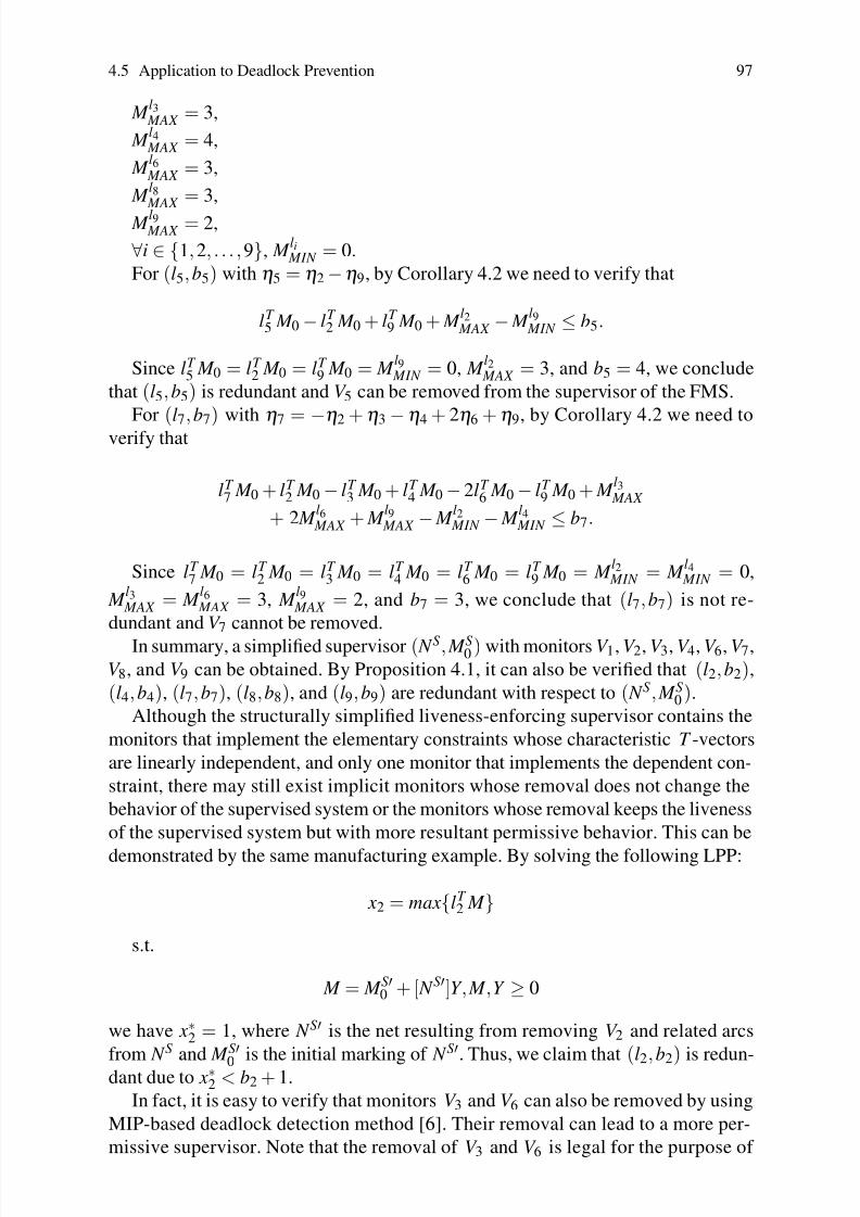
8/4/2019 Li Z., Zhou M. Deadlock Resolution in Automated Manufacturing Systems - A Novel Petri Net Approach
http://slidepdf.com/reader/full/li-z-zhou-m-deadlock-resolution-in-automated-manufacturing-systems-a-novel 112/249
4.5 Application to Deadlock Prevention 97
M l3
MAX = 3,
M l4
MAX = 4,
M l6
MAX = 3,
M l8
MAX = 3,
M l9 MAX = 2,
∀i ∈ 1,2, . . . ,9, M li
MIN = 0.
For (l5,b5) with η5 = η2 −η9, by Corollary 4.2 we need to verify that
lT 5 M 0 − lT
2 M 0 + lT 9 M 0 + M
l2 MAX − M
l9 MIN ≤ b5.
Since lT 5 M 0 = lT
2 M 0 = lT 9 M 0 = M
l9 MIN = 0, M
l2 MAX = 3, and b5 = 4, we conclude
that (l5,b5) is redundant and V 5 can be removed from the supervisor of the FMS.
For (l7,b7) with η7 =−η2 +η3
−η4 + 2η
6+η9, by Corollary 4.2 we need to
verify that
lT 7 M 0 + lT
2 M 0 − lT 3 M 0 + lT
4 M 0 − 2lT 6 M 0 − lT
9 M 0 + M l3
MAX
+ 2 M l6
MAX + M l9
MAX − M l2
MIN − M l4
MIN ≤ b7.
Since lT 7 M 0 = lT
2 M 0 = lT 3 M 0 = lT
4 M 0 = lT 6 M 0 = lT
9 M 0 = M l2
MIN = M l4
MIN = 0,
M l3
MAX = M l6
MAX = 3, M l9
MAX = 2, and b7 = 3, we conclude that (l7,b7) is not re-
dundant and V 7 cannot be removed.
In summary, a simplified supervisor ( N S, M S0 ) with monitors V 1, V 2, V 3, V 4, V 6, V 7,V 8, and V 9 can be obtained. By Proposition 4.1, it can also be verified that (l2,b2),
(l4,b4), (l7,b7), (l8,b8), and (l9,b9) are redundant with respect to ( N S, M S0 ).
Although the structurally simplified liveness-enforcing supervisor contains the
monitors that implement the elementary constraints whose characteristic T -vectors
are linearly independent, and only one monitor that implements the dependent con-
straint, there may still exist implicit monitors whose removal does not change the
behavior of the supervised system or the monitors whose removal keeps the liveness
of the supervised system but with more resultant permissive behavior. This can be
demonstrated by the same manufacturing example. By solving the following LPP:
x2 = maxlT 2 M
s.t.
M = M S′0 + [ N S′]Y , M ,Y ≥ 0
we have x∗2 = 1, where N S′ is the net resulting from removing V 2 and related arcs
from N S and M S′0
is the initial marking of N S′. Thus, we claim that (l2,b2) is redun-
dant due to x∗2 < b2 + 1.
In fact, it is easy to verify that monitors V 3 and V 6 can also be removed by using
MIP-based deadlock detection method [6]. Their removal can lead to a more per-
missive supervisor. Note that the removal of V 3 and V 6 is legal for the purpose of

8/4/2019 Li Z., Zhou M. Deadlock Resolution in Automated Manufacturing Systems - A Novel Petri Net Approach
http://slidepdf.com/reader/full/li-z-zhou-m-deadlock-resolution-in-automated-manufacturing-systems-a-novel 113/249
98 4 Monitor Implementation of GMECs
deadlock controls, i.e., the resultant system remains live. However, the removal of
monitors by the MIP-based method may violate the GMECs represented by (4.15).
Specifically, the supervisor with monitors V 1, V 3, and V 6 has 11 reachable states
and the one only with V 1 has 24 reachable states.
4.6 Some Further Results About S4R Nets
S4R represents an important subclass of Petri nets that can model a large class of
FMSs. In this section, the redundancy decision conditions of a dependent constraint
in an S4R stated by Corollaries 4.1 and 4.2 and their related results can be simplified
by the fact that its operation places are unmarked at the initial marking. In what
follows, ( N , M 0
) is used to represent an S4R where there is no confusion.
Corollary 4.3. Let (l,b) be a strongly dependent constraint with η = ∑ni=1 aiηi and
l = ∑ni=1 aili in ( N , M 0). (l,b) is redundant if
n
∑i=1
ai M li
MAX ≤ b.
Proof. By Corollary 4.1, this follows from the fact that (∪ni=1||li||)∪(||l||) ⊆ P A and
∀ p
∈P A, M 0( p) = 0.
⊓⊔Corollary 4.4. Let (l,b) be a weakly dependent constraint in ( N , M 0) with η =
∑ni=1 aiηi −∑m
j=1 a jη j and l = ∑ni=1 aili −∑m
j=1 a jl j . It is redundant if
n
∑i=1
ai M li
MAX ≤ b.
Proof. From Corollary 4.2, it is redundant if
lT
M 0 −n
∑i=1ail
T
i M 0 +
m
∑ j=1a jl
T
j M 0 +
n
∑i=1ai M
li
MAX −m
∑ j=1a j M
l j
MIN ≤ b.
According to the definition of an S4R, ∀ p ∈ P A, M 0( p) = 0. We have lT M 0 =
∑ni=1 ailT
i M 0 = ∑m j=1 a jlT
j M 0 = ∑m j=1 a j M
l j
MIN = 0. Hence, this result is true. ⊓⊔
This result indicates that in an S4R the redundancy of a weakly dependent
constraint has nothing to do with ∑m j=1 a jη j. Consequently, if (l,b) is (weakly or
strongly) dependent, its redundancy depends on (l1,b1), (l2,b2), . . ., and (ln,bn)only. Furthermore, we have the following results.
Corollary 4.5. Let (l,b) be a strongly dependent constraint in ( N , M 0) with η =
∑ni=1 aiηi and l = ∑
ni=1 aili. (l,b) is redundant if

8/4/2019 Li Z., Zhou M. Deadlock Resolution in Automated Manufacturing Systems - A Novel Petri Net Approach
http://slidepdf.com/reader/full/li-z-zhou-m-deadlock-resolution-in-automated-manufacturing-systems-a-novel 114/249
4.6 Some Further Results About S4R Nets 99
n
∑i=1
ai M limax ≤ b.
Proof. It is true by Theorem 4.3 since∀
p
∈ ||l
|| ∪(∪
n
i=1||li
||), M 0( p) = 0.
⊓⊔Corollary 4.6. Let (l,b) be a weakly dependent constraint in ( N , M 0) with η =
∑ni=1 aiηi −∑m
j=1 a jη j and l = ∑ni=1 aili −∑m
j=1 a jη j. (l,b) is redundant if
n
∑i=1
ai M limax ≤ b.
Corollary 4.7. Let (l,b) be a strongly dependent constraint in ( N , M 0) with η =
∑
n
i=1 aiηi and l = ∑
n
i=1 aili. ∀i ∈ Nn , monitor V i is added to enforce (li,bi). (l,b) isimplicitly enforced if
n
∑i=1
aibi ≤ b.
Proof. After V i is added, (li,bi) is hence enforced. The resultant net with these mon-
itors V 1 − V n is denoted by ( N S, M S0 ). This indicates the truth of bi ≥ M limax, where
M limax = max
lT
i
M | M
∈ R( N S, M S
0)
. ∑n
i=1aibi
≤b implies ∑
n
i=1ai M
limax
≤b.
⊓⊔Corollary 4.8. Let (l,b) be a weakly dependent constraint in ( N , M 0) with η =
∑ni=1 aiηi −∑m
j=1 a jη j and l = ∑ni=1 aili −∑m
j=1 a jl j. ∀i ∈ Nn , monitor V i is added
such that (li,bi) is enforced. (l,b) is implicitly enforced if
n
∑i=1
aibi ≤ b.
Proof. It follows immediately from Corollary 4.6.⊓⊔
Example 4.12. For the FMS example in Fig. 4.7, (l5,b5) is weakly dependent with
η5 =η2 −η9. Suppose that V 2 is added to enforce (l2,b2). Then, (l5,b5) is implicitly
enforced since b2 < b5. Furthermore, (l7,b7) is weakly dependent with η7 = −η2 +η3 −η4 + 2η6 +η9. Suppose that V 3, V 6 and V 9 are added to enforce (l3,b3), (l6,b6)and (l9,b9), respectively. However, (l7,b7) is not implicitly enforced since b3 +2b6 + b9 > b7.
In summary, for a set of GMECs to be enforced to ( N , M 0) for deadlock control
purpose by the policy in [40], the redundancy of a dependent constraint can be sim-
ply determined by the truth of an inequality. From the computational point of view,
the methodology proposed in this section is much more efficient. Next a parameter-
ized and more general result concerning the redundancy of a dependent constraint
is shown.

8/4/2019 Li Z., Zhou M. Deadlock Resolution in Automated Manufacturing Systems - A Novel Petri Net Approach
http://slidepdf.com/reader/full/li-z-zhou-m-deadlock-resolution-in-automated-manufacturing-systems-a-novel 115/249
100 4 Monitor Implementation of GMECs
Theorem 4.12. Let (l,b) be a weakly or strongly dependent constraint in ( N , M 0).
It is redundant if
n
∑i=1
aiξi
≥
n
∑i=1
aibi
−b.
Proof. It follows from Corollaries 4.5, 4.6–4.8. ⊓⊔This result indicates that a dependent constraint can be made redundant by prop-
erly setting the control depth variables of elementary constraints even if ∑ni=1 aibi ≤
b is not true.
Let ( L, B) be a set of GMECs in ( N , M 0), (li,bi), i ∈ Nn, be elementary con-
straints, and (l j,b j), j ∈ n + 1,n + 2, . . . ,m, be dependent constraints. The control
depth variables of the elementary constraints can be decided by solving the follow-
ing LPP once monitors V 1 − V n are explicitly added:
minn
∑i=1
ξi
s.t.
n
∑i=1
aiξi ≥n
∑i=1
aibi −b j,ai ≥ 0, j = n + 1,n + 2, . . . ,m.
0 ≤ ξi ≤ bi.
The existence of an optimal solution indicates that a set of GMECs can be en-
forced by using a set of monitors that are explicitly added for elementary constraints
whose number is bounded by the smaller of place and transition counts.
Example 4.13. For the FMS example in Fig. 4.7, the control depth variables of the
elementary constraints can be decided by solving the following LPP:
min x = ξ1 +ξ2 +ξ3 +ξ4 +ξ6 +ξ8 +ξ9
s.t.
ξ2 ≥ b2 − b5 = −3,
ξ3 + 2ξ6 +ξ9 ≥ b3 + 2b6 + b9 − b7 = 2,
0 ≤ ξ1 ≤ b1, 0 ≤ ξ2 ≤ b2, 0 ≤ ξ3 ≤ b3, 0 ≤ ξ4 ≤ b4,
0 ≤ ξ6 ≤ b6, 0 ≤ ξ8 ≤ b8, 0 ≤ ξ9 ≤ b9,
b1 = 1, b2 = 1, b3 = 1, b4 = 3, b5 = 4, b6 = 1, b7 = 3, b8 = 3, and b9 = 2.
This problem has an optimal solution x∗ = 1, implying that the control depth
variable ξ1 = ξ2 = ξ3 = ξ4 = ξ8 = ξ9 = 0, and ξ6 = 1. That is to say, all dependent
constraints are redundant if monitors are added for the elementary constraints withtheir control depth variables being zero except ξ6.

8/4/2019 Li Z., Zhou M. Deadlock Resolution in Automated Manufacturing Systems - A Novel Petri Net Approach
http://slidepdf.com/reader/full/li-z-zhou-m-deadlock-resolution-in-automated-manufacturing-systems-a-novel 116/249
4.7 Identification of Elementary Constraints 101
4.7 Identification of Elementary Constraints
The results in Sect. 4.6 indicate that the redundancy conditions of a dependent con-
straint (l,b) are easily satisfied when b is large and bi (i
∈Nn) is small, where (l1,b1)
− (ln,bn) are the elementary constraints of (l,b). This section develops an algorithmto identify a set of elementary constraints such that the redundancy condition of a
dependent constraint is easily satisfied without increasing the control depth vari-
ables of its elementary constraints. Let ( N , M 0) be a Petri net with N = (P,T ,F ,W ).
Without loss of generality, we assume that any two vectors in [η] are not identical.
Algorithm 4.1 Identification of elementary constraints
Input: ( L, B) = (li,bi)|i ∈ NnOutput: L E , a set of elementary constraints
1: Find [η ] from ( L, B)2: m := rank ([η ])3: By the merge sort algorithm, sort the sequence b1, b2, · · ·, and bn to be bk 1 , bk 2 ,
. . ., and bk n in an ascending order, where k 1,k 2, . . . ,k n = Nn
4: for j = 1 to n do
5: χ j := ηk j
6: end for
7: L E := (lk 1 ,bk 1 )8: A := [ χ 1]T
9: i := 2
10: while (m = 1) do
11: for i = 2 to n do
12: A E := [ AT | χ i]T
13: L E := L E ∪(l,b)|η = χ i14: while (rank ( A E ) = m) do
15: if rank ( A E ) − rank ( A) = 0 then
16: L E := L E \(l,b)|η = χ i17: i := i + 1
18: else
19: A := A E
20: i := i + 1
21: end if
22: end while
23: i := n + 1
24: end for
25: end while
26: Output L E
This algorithm is similar to the one that identifies a set of elementary siphons in
Sect. 3.6 of Chap. 3. The complexity of this algorithm is O(2n|P||T |2 + n lg n).
Example 4.14. For the set of GMECs in the FMS example in Sect. 4.6, this algo-
rithm outputs L E = (l1,b1),(l2,b2),(l3,b3),(l4,b4),(l6,b6),(l8,b8),(l9,b9).

8/4/2019 Li Z., Zhou M. Deadlock Resolution in Automated Manufacturing Systems - A Novel Petri Net Approach
http://slidepdf.com/reader/full/li-z-zhou-m-deadlock-resolution-in-automated-manufacturing-systems-a-novel 117/249
102 4 Monitor Implementation of GMECs
4.8 Bibliographical Remarks
As an important class of control specifications in the supervisory control of DES,
linear inequality constraints are first studied in [32]. They are also extensively in-
vestigated in a Petri net formalism. The work along this direction can be foundin [3,4,9,12,13,30,36,38]. Recent tutorials and survey papers are presented by Ior-
dache and Antsaklis [25, 27]. A good reference is the book by Moody and Antsak-
lis [37]. The work in [7] develops a systematic method to minimize the set of mon-
itors for forbidden-state problems in safe Petri nets.
Problems
4.1. Let (l1,b1) ≡ M ( p2) + M ( p6) ≤ 4, (l2,b2) ≡ M ( p3) + M ( p5) ≤ 4, (l3,b3) ≡ M ( p2) + M ( p3) + M ( p5) + M ( p6) ≤ 6, (l4,b4) ≡ 3 M ( p3) + 2 M ( p4) ≤ 8, (l5,b5) ≡ M ( p2) + M ( p4) + M ( p6) ≤ 5, (l6,b6) ≡ 3 M ( p2) + 4 M ( p5) ≤ 12, and (l7,b7) ≡ M ( p2) + M ( p5) + M ( p6) + M ( p7) ≤ 10 be a set of GMECs to the Petri net shown
in Fig. 4.8.
1. Find a set of elementary constraints by the algorithm in Sect. 4.7;
2. Try to find a set of control depth variables of the elementary constraints under
which dependent constraints are implicitly enforced;
3. Discuss the condition under which the dependent constraints cannot be implicitlyenforced by adding monitors for elementary constraints only.
p 1
t 2
t 3
t 1
p 3
p 2
t 4
p 4
p 1 0
8
t 7
t 6
t 8
p 8
p 7
p 6
t 5
p 5
p 1 1
p 9
8
Fig. 4.8 A Petri net ( N , M 0)

8/4/2019 Li Z., Zhou M. Deadlock Resolution in Automated Manufacturing Systems - A Novel Petri Net Approach
http://slidepdf.com/reader/full/li-z-zhou-m-deadlock-resolution-in-automated-manufacturing-systems-a-novel 118/249
References 103
4.2. Extend the results in this chapter to a Petri net with uncontrollable and unob-
servable transitions. The reader is referred to the work by Giua, Moody, and Ior-
dache [9, 29, 36–38].
4.3. Discuss the possibility of applying the results in this chapter to other classes
of control specifications such as constraints involving firing vectors and time, anddisjunction of inequality constraints. These control specifications are extensively
investigated by Iordache et al. [14–28].
References
1. Basile, F., Chiacchio, P., Giua, A. (1998) Supervisory control of Petri nets based on subopti-
mal monitor places. In Proc. IEE Int. Workshop on Discrete Event Systems, pp.85–87.2. Basile, F., Chiacchio, P. (2001) Optimal Petri net monitor design. In Synthesis and Contorl of
Discrete Event Systems,B. Cailaud, X. Xie, Ph. Darondeau, and L. Lavagno (Eds.), Boston,
MA: Kluwer, pp.141–154.
3. Basile, F., Carbone, C., Chiacchio, P. (2003) Petri net controllers to enforce disjunction of
GMECs. In Proc. IEEE Int. Conf. on Robotics and Automation, pp.1440–1445.4. Basile, F., Chiacchio, P., Giua, A. (2006) Suboptimal supervisory control of Petri nets in
presence of uncontrollable transitions via monitor places. Automatica, vol.42, no.6, pp.995–
1004.
5. Basile, F., Chiacchio, P., Giua, A. (2007) An optimization approach to Petri net monitor de-
sign. IEEE Transactions on Automatic Control, vol.52, no.2, pp.306–311.
6. Chu, F., Xie, X.L. (1997) Deadlock analysis of Petri nets using siphons and mathematicalprogramming. IEEE Transactions on Robotics and Automation, vol.13, no.6, pp.793–804.7. Dideban, A., Alla, H. (2007) Determination of minimal sets of control places for safe Petri
nets. In Proc. American Control Conference, New York City, USA, pp.4975–4980.
8. Ezpeleta, J, Colom, J.M., Martinez, J. (1995) A Petri net based deadlock prevention policy
for flexible manufacturing systems. IEEE Transactions on Robotics and Automation, vol.11,
no.2, pp.173–184.9. Giua, A., DiCesare, F., Silva, M. (1992) Generalized mutual exclusion constraints on nets
with uncontrollable transitions. In Proc. IEEE Int. Conf. on Systems, Man, and Cybernetics,
pp.974–979.10. Giua, A., DiCesare, F., Silva, M. (1993) Petri net supervisors for generalized mutual exclusion
constraints. In Proc. 12th IFAC World Congress, pp.267–270.11. Giua, A. Seatzu, C. (2001) Supervisory control of railway networks with Petri nets. In Proc.
40th IEEE Int. Conf. on Decision and Control, pp.5004–5009.
12. Holloway, L.E., Krogh, B.H. (1990) Synthesis of feedback control logic for a class of con-
trolled Petri nets. IEEE Transactions on Automatic Control, vol.35, no.5, pp.514–523.
13. Holloway, L.E., Krogh, B.H. (1992) On closed-loop liveness of discrete-event systems un-
der maximally permissive control. IEEE Transactions on Automatic Control, vol.37, no.5,
pp.692–697.
14. Iordache, M.V., Moody, J.O., Antsaklis, P.J. (2000) Method for the synthesis of deadlock pre-
vention controllers in systems modeled by Petri nets. In Proc. American Control Conference,
pp.3167–3171.
15. Iordache, M.V., Antsaklis, P.J. (2001) T-liveness enforcement in Petri nets based on structural
net properties. In Proc. IEEE Conf. on Decision and Control, pp.4984–4989.16. Iordache, M.V., Moody, J.O., Antsaklis, P.J. (2001) A method for the synthesis of liveness
enforcing supervisors in Petri nets. In Proc. American Control Conference, pp.4943–4948.
17. Iordache, M.V., Antsaklis, P.J. (2002) Synthesis of supervisors enforcing general linear vector
constraints in Petri nets. In Proc. American Control Conference, pp.154–159.

8/4/2019 Li Z., Zhou M. Deadlock Resolution in Automated Manufacturing Systems - A Novel Petri Net Approach
http://slidepdf.com/reader/full/li-z-zhou-m-deadlock-resolution-in-automated-manufacturing-systems-a-novel 119/249
104 4 Monitor Implementation of GMECs
18. Iordache, M.V., Moody, J.O., Antsaklis, P.J. (2002) Synthesis of deadlock prevention supervi-
sors using Petri nets. IEEE Transactions on Robotics and Automation, vol.18, no.1, pp.59–68.
19. Iordache, M.V., Antsaklis, P.J. (2003) Design of T-Liveness enforcing supervisors in Petri
nets. IEEE Transactions on Automatic Control, vol.48, no.11, pp.1962–1974.
20. Iordache, M.V., Antsaklis, P.J. (2003) Synthesis of supervisors enforcing general linear con-
straints in Petri nets. IEEE Transactions on Automatic Control, vol.48, no.11, pp.2036–2039.21. Iordache, M.V., Antsaklis, P.J. (2003) Decentralized control of Petri nets with constraint trans-
formations. In Proc. American Control Conference, pp.314–319.
22. Iordache, M.V., Antsaklis, P.J. (2003) Admissible decentralized control of Petri nets. In Pro.
American Control Conference, pp.332–337.
23. Iordache, M.V. (2003) Methods for the Supervisory Control of Concurrent Systems Based on
Petri Net Abstractions. Doctoral Dissertation, University of Notre Dame.
24. Iordache, M.V., Antsaklis, P.J. (2004) Resilience to failures and reconfigurations in the super-
vision based on place invariants. In Proc. American Control Conference, pp.4477–4482.
25. Iordache, M.V., Antsaklis, P.J. (2004) Supervision based on place invariants: A survey. Tech-
nical Report of the ISIS Group, ISIS-2004-003, University of Notre Dame.
26. Iordache, M.V., Antsaklis, P.J. (2005) A structural approach to the enforcement of languageand disjunctive constraints. In Proc. American Control Conference, pp.3920–3925.
27. Iordache, M.V., Antsaklis, P.J. (2006) Supervision based on place invariants: A survey. Dis-
crete Event Dynamic Systems: Theory and Applications, vol.16, no.4, pp.451–492.
28. Iordache, M.V., Antsaklis, P.J. (2006) Decentralized supervision of Petri nets. IEEE Transac-
tions on Automatic Control, vol.51, no.2, pp.376–381.
29. Iordache, M.V., Antsaklis, P.J. (2006) Supervisory Control of Concurrent Systems: A Petri
Net Structural Approach. Berlin: Springer.
30. Krogh, B.H., Holloway, L.E. (1991) Synthesis of feedback control logic for discrete manu-
facturing systems. Automatica, vol.27, no.4, pp.641–645.
31. Li, Y., Wonham, W.M. (1993) Control of vector discrete-event systems. I. The base model.
IEEE Transactions on Automatic Control, vol.38, no.8, pp.1214–1227.
32. Li, Y., Wonham, W.M. (1994) Control of vector discrete-event systems. II. Controller synthe-
sis. IEEE Transactions on Automatic Control, vol.39, no.3, pp.512–531.
33. Li, Y., Wonham, W.M. (1995) Concurrent vector discrete-event systems. IEEE Transactions
on Automatic Control, vol.40. no.4, pp.628–638.
34. Li, Z.W., Zhou, M.C. (2004) Elementary siphons of Petri nets and their application to dead-
lock prevention in flexible manufacturing systems. IEEE Transactions on Systems, Man, and
Cybernetics, Part A, vol.34, no.1, pp.38–51.
35. Li, Z.W., Zhou, M.C. (2006) Clarifications on the definitions of elementary siphons of Petri
nets. IEEE Transactions on Systems, Man, and Cybernetics, Part A, vol.36, no.6, pp.1227–
1229.
36. Moody, J.O., Lemmon, M.D., Antsaklis, P.J. (1996) Supervisory control of Petri nets with un-
controllable and unobservable transitions. In Proc. 35th IEEE Conf. on Control and Decision,
pp.4433–4438.
37. Moody, J.O., Antsaklis, P.J. (1998) Supervisory Control of Discrete Event Systems Using Petri
Nets. Boston, MA: Kluwer.
38. Moody, J.O., Antsaklis, P.J. (2000) Petri net supervisors for DES with uncontrollable and
unobservable transitions. IEEE Transactions on Automatic Control, vol.45, no.3, pp.462–476.
39. Park, J. (2000) Structural analysis and control of resource allocation systems using Petri nets.
PhD thesis, Georgia Institute of Technology, Atlanta, GA.
40. Park, J., Reveliotis, S.A. (2001) Deadlock avoidance in sequential resource allocation systems
with multiple resource acquisitions and flexible routings. IEEE Transactions on Automatic
Control, vol.46, no.10, pp.1572–1583.
41. Reveliotis, S.A. (2007) Implicit siphon control and its role in the liveness-enforcing super-vision of sequential resource allocation systems. IEEE Transactions on Systems, Man, and
Cybernetics, Part A, vol.37, no.3, pp.319–328.
42. Tittus, M., Egardt, B. (1999) Hierarchical supervisory control for batch processes. IEEE
Transactions on Control System Technology, vol.7, no.5, pp.542–554.

8/4/2019 Li Z., Zhou M. Deadlock Resolution in Automated Manufacturing Systems - A Novel Petri Net Approach
http://slidepdf.com/reader/full/li-z-zhou-m-deadlock-resolution-in-automated-manufacturing-systems-a-novel 120/249
References 105
43. Tricas, F. (2003) Deadlock Analysis, Prevention and Avoidance in Sequential Resource Allo-
cation Systems, Ph.D Dissertation, University of Zaragoza, Spain.
44. Yamalidou, E., Kantor, J. (1991) Modeling an optimal control of discrete-event chemical
processes using Petri nets. Computers and Chemical Engineering, vol.15, no.7, pp.503–519.
45. Yamalidou, E., Moody, J.O., Antsaklis, P.J. (1996) Feedback control of Petri nets based on
place invariants. Automatica, vol.32, no.1, pp.15–28.46. Zhou, M.C., DiCesare, F. (1991) Parallel and sequential exclusions for Petri net modeling for
manufacturing systems. IEEE Transactions on Robotics and Automation, vol.7, no.4, pp.515–
527.
47. Zhou, M.C., DiCesare, F. (1993) Petri Net Synthesis for Discrete Event Control of Manufac-
turing Systems. Boston, MA: Kluwer.

8/4/2019 Li Z., Zhou M. Deadlock Resolution in Automated Manufacturing Systems - A Novel Petri Net Approach
http://slidepdf.com/reader/full/li-z-zhou-m-deadlock-resolution-in-automated-manufacturing-systems-a-novel 121/249
Chapter 5
Deadlock Control Based on Elementary Siphons
Abstract This chapter first reviews a classical deadlock prevention policy for au-
tomated manufacturing systems, which is usually considered to be the first that uti-
lizes structural theory of Petri nets to design a liveness-enforcing (Petri net) super-
visor. To reduce the computational complexity to design deadlock-free supervisors,
a mixed-integer-programming based deadlock detection method is presented. Then,
a number of deadlock prevention policies are introduced by using the controllabil-
ity results of elementary and dependent siphons, which are applicable to ordinary
and generalized Petri net models. This chapter shows that the deadlock prevention
policies based on elementary siphons can reduce the computational and structural
complexity and improve the behavioral permissiveness of the liveness-enforcing
monitor-based supervisors. Importantly, some interesting or open problems in this
area are listed at the end of this chapter.
5.1 Introduction
This chapter presents a number of deadlock prevention policies. They are based on
the concepts of strict minimal and elementary siphons. They can be applied to thedeadlock resolution in resource allocation systems that are modeled with ordinary
and generalized Petri nets. First, we review the seminal work [16] in this area. It
develops a deadlock control policy that prevents strict minimal siphons from being
unmarked by adding monitors for them. Then, a number of deadlock prevention
approaches by using elementary siphons are presented.
5.2 Some Application Subclasses of Petri Nets
This section defines a number of subclasses of Petri nets, which can model real-life
automated flexible manufacturing systems, a typical and important class of resource
107

8/4/2019 Li Z., Zhou M. Deadlock Resolution in Automated Manufacturing Systems - A Novel Petri Net Approach
http://slidepdf.com/reader/full/li-z-zhou-m-deadlock-resolution-in-automated-manufacturing-systems-a-novel 122/249
108 5 Deadlock Control Based on Elementary Siphons
allocation systems in the contemporary technical domain. The policies presented
in this chapter can be applied to them. First a class of Petri nets called S3PR is
defined [16]. It stands for system of simple sequential processes with resources.
Definition 5.1. Let ( N 1, M 1) and ( N 2, M 2) be two Petri nets with N 1 = (P1,T 1,F 1,W 1)and N 2 = (P2,T 2,F 2,W 2), where P1 ∩ P2 = PC = / 0 and T 1 ∩ T 2 = / 0. ( N , M ) with
N = (P,T ,F ,W ) is said to be the resultant net of composing ( N 1, M 1) and ( N 2, M 2)via the set of shared places PC iff (1) P = P1 ∪ P2, T = T 1 ∪ T 2, F = F 1 ∪ F 2, and
W ( x, y) = W i( x, y) if ( x, y) ∈ F i, i = 1,2; and (2) ∀ p ∈ P1 \ PC , M ( p) = M 1( p),
∀ p ∈ P2 \ PC , M ( p) = M 2( p), and ∀ p ∈ PC , M ( p) = max M 1( p), M 2( p).
The two nets N 1 and N 2 satisfying P1 ∩ P2 = PC = / 0 and T 1 ∩T 2 = / 0 in Definition
5.1 are said to be composable via shared places. Their composition is denoted by
N 1
N 2.
Example 5.1. Two nets ( N 1, M 1) and ( N 2, M 2) are shown in Fig. 5.1a and Fig. 5.1b,
respectively, where P1 = p1− p4, p9− p11, T 1 = t 1−t 4, P2 = p5− p11, and
T 2 = t 5−t 8. Since P1 ∩ P2 = p9, p10, p11 and T 1 ∩T 2 = / 0, ( N 1, M 1) and ( N 2, M 2)are composable. As shown in Fig. 5.1(c), the net resulting from the composition
of ( N 1, M 1) and ( N 2, M 2) is denoted by ( N , M ) where P = P1 ∪ P2 = p1− p11,
T = T 1 ∪ T 2 = t 1−t 8, M ( p1) = M 1( p1) = 10, M ( p2) = M 1( p2) = 0, M ( p3) = M 1( p3) = 0, M ( p4) = M 1( p4) = 0, M ( p5) = M 2( p5) = 10, M ( p6) = M 2( p6) = 0,
M ( p7) = M 2( p7) = 0, M ( p8) = M 2( p8) = 0, M ( p9) = max M 1( p9), M 2( p9) = 2,
M ( p10
) = max M
1( p
10), M
2( p
10)
= 2, and M ( p11
) = max M
1( p
11), M
2( p
11)
=3.
Definition 5.2. A simple sequential process (S2P) is a Petri net N = (P A ∪ p0,T ,F )where (1) P A = / 0 is called the set of operation places; (2) p0 ∈ P A is called the idle
process place; (3) N is a strongly connected state machine; and 4) every circuit of N
contains place p0.
Definition 5.3. A simple sequential process with resources (S2PR) is a Petri net
N = (
p0
∪P
A ∪P
R,T ,
F )
such that:
1. The subnet generated by X = P A ∪ p0∪ T is an S2P.
2. P R = / 0 and (P A ∪ p0) ∩ P R = / 0.
3. ∀ p ∈ P A, ∀t ∈• p, ∀t ′ ∈ p•, ∃r p ∈ P R, •t ∩ P R = t ′• ∩ P R = r p.
4. The following statements are verified: (a) ∀r ∈ P R, ••r ∩ P A = r •• ∩ P A = / 0 and
(b) ∀r ∈ P R, •r ∩ r • = / 0.
5. ••( p0) ∩ P R = ( p0)•• ∩ P R = / 0.
Note that •r represents place r ’s input transitions. ••r =∪
t ∈•
r •t is the set of all
input places of all input transitions of place r . Similarly, r •• = ∪t ∈r •t • represents
the set of all output places of all output transitions of place r . For example, in Fig.
5.1(c), • p9 = t 2,t 8 and •• p9 =•t 2 ∪ •t 8 = p2, p10, p8. p•9 = t 1,t 7 and p••
9 =t •1 ∪ t 7
• = p2, p10, p8. Clearly, •• p9 = p••9 .

8/4/2019 Li Z., Zhou M. Deadlock Resolution in Automated Manufacturing Systems - A Novel Petri Net Approach
http://slidepdf.com/reader/full/li-z-zhou-m-deadlock-resolution-in-automated-manufacturing-systems-a-novel 123/249
5.2 Some Application Subclasses of Petri Nets 109
( b )
p 9p 2
p 4
p 3
p 1 1
p 1 0
t 1
t 2
t 3
t 4
p 1
( a )
p 5
p 9 p 8
p 6
p 7
p 1 1
p 1 0
t 5
t 8
t 7
t 6
1 0 1 0
p 9
p 2
p 4
p 3
p 1 1
p 1 0
t 1
t 2
t 3
t 4
p 1
( c )
p 5
p 8
p 6
p 7
t 5
t 8
t 7
t 6
1 0 1 0
Fig. 5.1 (a) A Petri net ( N 1, M 1), (b) a Petri net ( N 2, M 2), and (c) the composed net ( N , M )
Definition 5.4. Let N = (P A ∪ p0∪ P R,T ,F ) be an S2PR. An initial marking M 0is called an acceptable initial marking for N iff (1) M 0( p0) ≥ 1, (2) M 0( p) = 0,
∀ p ∈ P A, and (3) M 0(r ) ≥ 1, ∀r ∈ P R. An S2PR with such a marking is said to be
acceptably marked.
Example 5.2. The net shown in Fig. 5.2(a) is an S2P, where p0 is the idle process
place and P A = p1− p6 is the set of operation places. It is easy to verify that the
net is a strongly connected state machine.

8/4/2019 Li Z., Zhou M. Deadlock Resolution in Automated Manufacturing Systems - A Novel Petri Net Approach
http://slidepdf.com/reader/full/li-z-zhou-m-deadlock-resolution-in-automated-manufacturing-systems-a-novel 124/249
110 5 Deadlock Control Based on Elementary Siphons
The net ( N 2, M 2) depicted in Fig. 5.2(b) is an S2PR extending from the S2P in Fig.
5.2(a), where P R = p7− p12 is the set of resource places. It meets the conditions
in Definitions 5.3 and 5.4. Hence, ( N 2, M 2) is an S2PR with an acceptable initial
marking.
p 3
p 1
p0
p 6
p 5
p 4
p 2
t 1
t 6
t 7
t 8
t 5
t 4
t 3
t 2
( a )
p 3
p 1
p0
p 6
p 5
p 4
p 2
t 1
t 6
t 7
t 8
t 5
t 4
t 3
t 2
p 8
p 1 0
p 9
p 1 1
p 1 2
p 7
( b )
1 0 1 0
Fig. 5.2 (a) An S2P ( N 1, M 1) with a state machine structure, (b) an S2PR ( N 2, M 2) with an accept-
able initial marking
Definition 5.5. A system of S2PR, called S3PR for short, is defined recursively as
follows:
1. An S2PR is an S3PR.
2. Let N i = (P Ai∪ p0
i ∪P Ri,T i,F i), i ∈ 1,2, be two S3PR such that (P A1
∪ p01)∩
(P A2∪ p0
2) = / 0, P R1∩ P R2
= PC = / 0, and T 1 ∩ T 2 = / 0. Then, the net N = (P A ∪P0 ∪ P R,T ,F ) resulting from the composition of N 1 and N 2 via PC defined as
follows: (1) P A = P A1∪ P A2
, (2) P0 = p01∪ p0
2, (3) P R = P R1∪ P R2
, (4) T =T 1 ∪ T 2, and (5) F = F 1 ∪ F 2 is also an S3PR.
In the sequel, an S3PR N composed of n S2PR N 1- N n, denoted by N = ni=1 N i,
is defined as follows: N = N 1 if n = 1; N = (
n−1i=1 N i)
N n if n > 1. N i is used to
denote the S2P from which the S2PR N i is formed. Transitions in (P0)• are calledsource transitions that represent the entry of raw materials when a manufacturing
system is modeled with an S3PR.

8/4/2019 Li Z., Zhou M. Deadlock Resolution in Automated Manufacturing Systems - A Novel Petri Net Approach
http://slidepdf.com/reader/full/li-z-zhou-m-deadlock-resolution-in-automated-manufacturing-systems-a-novel 125/249
5.2 Some Application Subclasses of Petri Nets 111
Definition 5.6. Let N be an S3PR. ( N , M 0) is called an acceptably marked S3PR iff
one of the following statements is true:
1. ( N , M 0) is an acceptably marked S2PR.
2. N = N 1
N 2, where ( N i, M 0i
) is an acceptably marked S3PR and
a. ∀i ∈ 1,2, ∀ p ∈ P Ai∪ p0
i , M 0( p) = M 0i( p).
b. ∀i ∈ 1,2, ∀r ∈ P Ri\PC , M 0(r ) = M 0i
(r ).
c. ∀r ∈ PC , M 0(r ) = max M 01(r ), M 02
(r ).
Example 5.3. The net ( N 1, M 1) shown in Fig. 5.1(a) is an S3PR if p1 is an idle pro-
cess place, p2− p4 are operation places, and p9− p11 are resource places. Likewise,
( N 2, M 2) shown in Fig. 5.1(b) is an S3PR if p5 is an idle process place, p6− p8 are
operation places, and p9− p11 are resource places. Since they have common resource
places, they are composable. Their composition leads to an S3
PR ( N , M ), as shownin Fig. 5.1(c). Since one can verify that it meets the conditions in Definition 5.6, the
net in Fig. 5.1(c) is an acceptably marked S3PR.
In what follows, when we talk about an S3PR, it is assumed to be acceptably
marked unless otherwise stated. For example, the net shown in Fig. 5.3 is an S3PR
if P0 = p1, p10, P R = p11− p15, and others are operation places. Specifically, we
have P A1= p2, p3, p5 − p7 and P A2
= p4, p8, p9. It is easy to verify that ( N , M 0)is acceptably marked.
p 1
p 5
p 3
t 4
t 3
p 6
t 5
p 7
p 4
p 9
t 1 1
t 9
t 1 0
p 8
p 2
t 6
5
p 1 1
t 1
t 2
3
p 1 0
p 1 5
p 1 4
p 1 3
p 1 2
t 8
t 7
Fig. 5.3 An S3PR net ( N , M 0)
Let S be a strict minimal siphon in an S3PR N = (P A ∪ P0 ∪ P R, T , F ). Ezpeleta
et al. [16] show that S does not contain idle places but consists of operation and

8/4/2019 Li Z., Zhou M. Deadlock Resolution in Automated Manufacturing Systems - A Novel Petri Net Approach
http://slidepdf.com/reader/full/li-z-zhou-m-deadlock-resolution-in-automated-manufacturing-systems-a-novel 126/249
112 5 Deadlock Control Based on Elementary Siphons
resource places only. As a result, S can be represented by S A ∪S R, where S R = S∩P R
and S A = S\S R, i.e., S A = S ∩ P A.
Definition 5.7. For r ∈ P R, H (r ) = ••r ∩P A, the operation places that use r , is called
the set of holders of r . Let [S] = (∪r ∈S
R H (r ))\
S. [S] is called the complementary set
of siphon S.
Suppose that S = r 1,r 2, p2, p3 is a strict minimal siphon in an S3PR, where r 1and r 2 are resource places, and p2 and p3 are operation places. If H (r 1) = p1, p2and H (r 2) = p3, p4, then we have complementary set [S] = ( p1, p2∪ p3, p4)\S = p1, p4.
The concept of the complementary set of a siphon plays an important role in the
development of the deadlock prevention policy in [16]. Intuitively, the complemen-
tary set of a siphon is a set of operation places that use the resources in it but are
excluded from it. That is to say, the operation places in the complementary set com-pete for the limited resources with those in the siphon. When the tokens initially
staying in the resource places of a siphon are completely held or “stolen” by the
places in its complementary set, the siphon is emptied. As is known, if a siphon
has no token, it remains free of tokens in the subsequent reachable markings. The
transitions in its postset are completely disabled, leading to deadlocks.
It is shown in [16] that a strict minimal siphon S in an S3PR can be emptied and
|S ∩ S R| > 1 is true. That is to say, a strict minimal siphon in an S3PR contains at
least two resource places.
Property 5.1. Let N = ni=1 N i = (P0 ∪ P A ∪ P R,T ,F ) be an S3PR consisting of n
simple sequential processes and S be a siphon in N .
1. Any p ∈ P Aiis associated with a minimal P-semiflow I p with support || I p|| =
P Ai∪ p0
i .
2. Any resource r ∈ P R is associated with a minimal P-semiflow I r such that || I r || =r ∪ H (r ).
3. ∀ p ∈ [S], ∃r ∈ S R, p ∈ H (r ) and ∀r ′ ∈ P R\r , p /∈ H (r ′).
4. [S]
∪S is the support of a P-semiflow of N .
5. [S] = ∪ni=1[S]i, where [S]i = [S] ∩ P Ai .
Example 5.4. Consider the S3PR in Fig. 5.3, where p01 = p1, P A1
= p2, p3, p5, p6,
p7, p02 = p10, and P A2
= p4, p8, p9. Clearly, S1 = p5, p9, p12, p13 is a strict min-
imal siphon. It does not contain idle places. Let S1 = S A1 ∪S R
1 . We have S A1 = p5, p9
and S R1 = p12, p13. Let σ = t 1t 2t 8t 9 and M 0[σ M 1. Siphon S1 is emptied under
marking M 1 = 4 p1 + p3 + p4 + 2 p10 + p11 + p14 + p15. Place p12 is a resource place
with H ( p12) = p3, p9. Place p13 is a resource place with H ( p13) = p4, p5. Com-
plementary set [S1] = H ( p12)
∪ H ( p13)
\S1=
p3, p9, p5, p4
\S1=
p3, p4
. Specifi-
cally, [S1] = [S1]1 ∪ [S1]2, where [S1]1 = p3 and [S1]2 = p4. The minimal P-
invariants associated with idle place p1 and resource place p12 are I p1= p1 + p2 +
p3 + p5 + p6 + p7 and I p12= p3 + p9 + p12, respectively.

8/4/2019 Li Z., Zhou M. Deadlock Resolution in Automated Manufacturing Systems - A Novel Petri Net Approach
http://slidepdf.com/reader/full/li-z-zhou-m-deadlock-resolution-in-automated-manufacturing-systems-a-novel 127/249
5.2 Some Application Subclasses of Petri Nets 113
Note that ∀ p ∈ P A ∪ P0 (∀r ∈ P R), || I p|| (|| I r ||) is a minimal siphon and trap that
is initially marked. Let Π be the set of strict minimal siphons in an S3PR. The
following result is from [16], indicating that an S3PR is live iff there is no siphon
that can be emptied.
Theorem 5.1. An S3PR ( N , M 0) is live iff ∀ M ∈ R( N , M 0) , ∀S ∈Π , M (S) > 0.
Next a more general class of Petri nets than S3PR nets is introduced. It is first
proposed in [25] and called ES3PR. It stands for extended S3PR.
Definition 5.8. An ES3PR is an ordinary connected self-loop-free Petri net N =n
i=1 N i = (P,T ,F ) where:
1. N i = (P Ai∪ p0
i ∪ P Ri,T i,F i), i ∈ Nn.
2. P = P A
∪P0
∪P R is a partition such that (1) P A =
∪ni=1P Ai
is called the set of
operation places, where ∀i, j ∈ Nn, i = j, P Ai = / 0 and P Ai ∩ P A j = / 0; (2) P0 =∪n
i=1 p0i is called the set of idle places; (3) P R = r 1,r 2, . . . ,r m|m ∈ N+ is
called the set of resource places.
3. T = ∪ni=1T i is called the set of transitions, where ∀i, j ∈ Nn, i = j, T i = / 0 and
T i ∩ T j = / 0.
4. ∀i ∈ Nn, the subnet N i generated by P Ai∪ p0
i ∪ T i is a strongly connected state
machine such that every circuit of the state machine contains idle place p0i .
5. ∀r ∈ P R, there exists a unique minimal P-semiflow I r ∈ N|P| such that r =
|| I r
|| ∩P R, P0
∩ || I r
||= / 0, P A
∩ || I r
|| = / 0, and
∀ p
∈ || I r
||, I r ( p) = 1.
6. P A = ∪r ∈P R (|| I r ||\r ).
Definition 5.9. An initial marking M 0 is acceptable for an ES3PR N = (P A ∪ P0 ∪P R,T ,F ) iff (1) ∀i ∈ Nn, M 0( p0
i ) > 0; (2) ∀ p ∈ P A, M 0( p) = 0; and (3) ∀r ∈ P R,
M 0(r ) > 0.
From their definitions, the difference between S3PR and ES3PR is that the usage
of the resources in the latter is more flexible than that in the former. Specifically,
each operation place in an S3PR needs one resource only. However, an operation
place in an ES3PR may need two or more resources.
Theorem 5.2. Let ( N , M 0) be an ES3PR. It is live iff no siphon can become empty.
The net shown in Fig. 5.4 is an ES3PR in which p2– p9 are operation places that
are initially unmarked, p1 and p10 are idle places, and the others are resource places.
It is not an S3PR. It is live since no siphon can be emptied during its evolution.
As a generalization of S3PR and ES3PR in [25] and [50], respectively, the defi-
nition of the class of systems of sequential systems with shared resources (S4R) is
given in [1, 3]. It allows multiple arcs between a resource place and transition. The
represented net models fall into the generalized Petri net class. However, an S4R
cannot model a manufacturing system with assembly and disassembly operations
since it is composed of a set of state machines where no synchronization structure
is allowed.

8/4/2019 Li Z., Zhou M. Deadlock Resolution in Automated Manufacturing Systems - A Novel Petri Net Approach
http://slidepdf.com/reader/full/li-z-zhou-m-deadlock-resolution-in-automated-manufacturing-systems-a-novel 128/249
114 5 Deadlock Control Based on Elementary Siphons
p 1
p 5
p 3
t 4
t 3
p 6
t 5
p 7
p 4
p 9
t 1 1
t 9
t 1 0
p 8
p 2
t 6
5
p 1 1
t 1
t 2
3
p 1 0
p 1 5
p 1 4
p 1 3
p 1 2
t 8
t 7
t 6t 1
t 9t 8
V S 2
t 8
t 1
VS 1t 6
t 1 0t 3
Fig. 5.4 An ES3PR ( N , M 0)
Definition 5.10. An S4R is a generalized connected self-loop-free Petri net N =
ni=1 N i = (P,T ,F ,W ) where:
1. N i = (P Ai∪ p0
i ∪ P Ri,T i,F i,W i), i ∈Nn.
2. P = P A ∪ P0 ∪ P R is a partition such that (1) P A = ∪ni=1P Ai
is called the set of
operation places, where ∀i, j ∈ Nn, i = j, P Ai= / 0 and P Ai
∩ P A j= / 0; (2) P0 =
∪ni=1 p0
i is called the set of idle places; (3) P R = ∪ni=1P Ri
= r 1,r 2, · · · ,r m|m ∈N+ is called the set of resource places.
3. T = ∪ni=1T i is called the set of transitions, where ∀i, j ∈ Nn, i = j, T i = / 0 and
T i ∩ T j = / 0.
4. ∀i ∈ Nn, the subnet N i generated by P Ai ∪ p0i ∪ T i is a strongly connected state
machine such that every circuit of the state machine contains idle place p0i .
5. ∀r ∈ P R, there exists a unique minimal P-semiflow I r ∈ N|P| such that r =|| I r || ∩ P R, P0 ∩ || I r || = / 0, P A ∩ || I r || = / 0, and I r (r ) = 1.
6. P A = ∪r ∈P R(|| I r ||\r ).
Definition 5.11. An initial marking M 0 is acceptable for an S4R N = (P A ∪ P0 ∪P R,T ,F ,W ) iff (1) ∀i ∈ Nn, M 0( p0
i ) > 0; (2) ∀ p ∈ P A, M 0( p) = 0; and (3) ∀r ∈ P R,
M 0(r )
≥max
I r ( p)
| p
∈P A
.
Example 5.5. The net shown in Fig. 4.5 is an S4R, where I r 1 = r 1 + p1 + 3 p2 + p6 is
the minimal P-semiflow associated with resource r 1. An acceptable initial marking
M 0 needs to satisfy M 0(r 1) ≥ 3.

8/4/2019 Li Z., Zhou M. Deadlock Resolution in Automated Manufacturing Systems - A Novel Petri Net Approach
http://slidepdf.com/reader/full/li-z-zhou-m-deadlock-resolution-in-automated-manufacturing-systems-a-novel 129/249
5.2 Some Application Subclasses of Petri Nets 115
The class of Petri nets defined above is alternatively named to be S4PR [51] by
different researchers. The following result from [1] concerns the liveness of an S4R.
Theorem 5.3. [1] Let ( N , M 0) be a marked S4 R net. It is live iff it satisfies the
max-cs property 1.
Theorem 5.4. [1, 51] Let S be a strict minimal siphon in an S4 R N = (P A ∪ P0 ∪P R,T ,F ,W ). Then S = S R ∪ S A satisfies S ∩ P R = S R = / 0 and S ∩ P A = S A = / 0.
Before the presentation of the complementary set of a siphon in a generalized
Petri net, a brief theory of multisets is given in order to recognize well the role
of the complementary sets of siphons in the development of deadlock prevention
policies for generalized Petri nets that are used to model automated manufacturing
systems. A multiset is a generalization of the concept of a set.
Definition 5.12. A multiset Ω , over a non-empty set A, is a mapping Ω : A → N+,which we represent as a formal sum ∑a∈ AΩ (a).a.
In multiset Ω , non-negative integer Ω (a) is the coefficient of element a ∈ A,
indicating the number of occurrences of a in Ω . It is said that a ∈ A belongs to
Ω , denoted by a ∈ Ω , if Ω (a) > 0. It does not belong to Ω , denoted by a ∈ Ω ,if Ω (a) = 0. Let Ω MS denote the set of all multisets over A and Ω 1 and Ω 2 be two
multisets in Ω MS . The basic operations on multisets are union, intersection, addition,
and difference, which are defined as follows.
Definition 5.13. Ω 1 ∪Ω 2 := ∑a∈ A maxΩ 1(a),Ω 2(a).a.
Definition 5.14. Ω 1 ∩Ω 2 := ∑a∈ A minΩ 1(a),Ω 2(a).a.
Definition 5.15. Ω 1 +Ω 2 := ∑a∈ A(Ω 1(a) +Ω 2(a)).a.
Definition 5.16. Ω 1 −Ω 2 := ∑a∈ A(Ω 1(a) − (Ω 1 ∩Ω 2)(a)).a.
A multiset without any element is denoted by / 0 as an empty set. A multiset
becomes a set if the multiplicity of every element is one.
Example 5.6. Ω 1 = a+ b, Ω 2 = 2a+b+c, and Ω 3 = 3a+2c are three multisets over
A = a,b,c. We have Ω 1 ∪Ω 2 = 2a + b + c, Ω 1 ∪Ω 3 = 3a + b + 2c, Ω 1 ∩Ω 3 = a,
Ω 2 ∩Ω 3 = 2a + c, Ω 1 +Ω 2 = 3a + 2b + c, Ω 1 −Ω 2 = / 0, Ω 3 −Ω 1 = 2a + 2c, and
Ω 3 −Ω 2 = a + c.
Definition 5.17. Let r be a resource place and S be a strict minimal siphon in an
S4R. The holder of resource r is defined as the difference of two multisets I r and r :
H (r ) = I r − r . As a multiset, T h(S) = ∑r ∈S R H (r ) −∑r ∈S R, p∈S A I r ( p). p is called the
complementary set of siphon S.
1 This result is unfortunately not correct since the max-cs property is found to be a sufficient but
not necessary condition for the liveness of an S4R. For details, the reader can be referred to [8],
where the controllability condition of siphons in a generalized Petri net is relaxed by introducing
the concept of max’-controlled siphons.

8/4/2019 Li Z., Zhou M. Deadlock Resolution in Automated Manufacturing Systems - A Novel Petri Net Approach
http://slidepdf.com/reader/full/li-z-zhou-m-deadlock-resolution-in-automated-manufacturing-systems-a-novel 130/249
116 5 Deadlock Control Based on Elementary Siphons
Definition 5.18. ||T h(S)|| = p| p ∈ ∪r ∈S R H (r ), p /∈ S is called the support of com-
plementary set T h(S) of siphon S.
It is easy to see that ||T h(S)|| ⊆ P A is true. Let ||T h(S)||i = ||T h(S)|| ∩ P Ai; we
have
||T h(S)
||=
∪ni=1
||T h(S)
||i. Let∑ p
∈||T h(S)
||hS( p) p denote T h(S). Clearly, hS( p)
indicates that siphon S loses hS( p) tokens if the number of tokens in p increases byone. hS( p) is called the risk coefficient of place p.
Example 5.7. The net shown in Fig. 5.5 is an S4R if p01 = p7, p0
2 = p11, P A1= p1–
p6, P A2= p8– p10, P R1
= p12– p15, and P R2= p12– p14. It has three strict
minimal siphons:
S1 = p3, p6, p9, p13, p14,
S2 = p2, p5, p10, p12, p13,
S3 = p3, p6, p10, p12, p13, p14.
We have
I p12= 2 p1 + p10 + p12,
I p13= p2 + p5 + p9 + p13,
I p14= p3 + p6 + p8 + p14,
I p15= p4 + p15,
H ( p12) = 2 p1 + p10,
H ( p13) = p2 + p5 + p9,
H ( p14) = p3 + p6 + p8.
Furthermore, the complementary sets and their supports of siphons S1–S3 are:
T h(S1) = ( H ( p13) + H ( p14))
−( p3 + p6 + p9) = p2 + p5 + p8,
T h(S2) = ( H ( p12) + H ( p13)) − ( p2 + p5 + p10) = 2 p1 + p9,
T h(S3) = ∑14i=12 H ( pi) − ( p3 + p6 + p10) = 2 p1 + p2 + p5 + p8 + p9,
||T h(S1)|| = p2, p5, p8,
||T h(S2)|| = p1, p9,
||T h(S3)|| = p1, p2, p5, p8, p9.
For T h(S2), we have the risk coefficients of p1 and p9 are hS2( p1) = 2 and
hS2( p9) = 1, respectively. It is easy to see that two tokens are removed from S2
(in fact from p12) if the number of tokens in p1 increases by one.
Note that where there is no confusion, we often use [S] to denote the set of placesin T h(S) as well as T h(S) for convenience and clarity.
5.3 An MIP-Based Deadlock Detection Method
Let ( N , M ) be an ordinary net with N = (P,T ,F ) and S be the maximal empty siphon
at M , i.e., ∀ p /∈ S, M ( p)> 0. As shown in [9], finding S in N is the solution of
a mixed-integer-programming (MIP) problem.
∀ p /
∈S, let v p = 1 and
∀t /∈
S•, let
zt = 1.
It is easy to see that any p with v p = 1 and any t with zt = 1 are removed from
the net. Since S is a siphon, we have that ∀t ∈ p•, v p = 0 implies zt = 0 and ∀ p ∈ t •,
zt = 1 implies the truth of v p = 1. This leads to
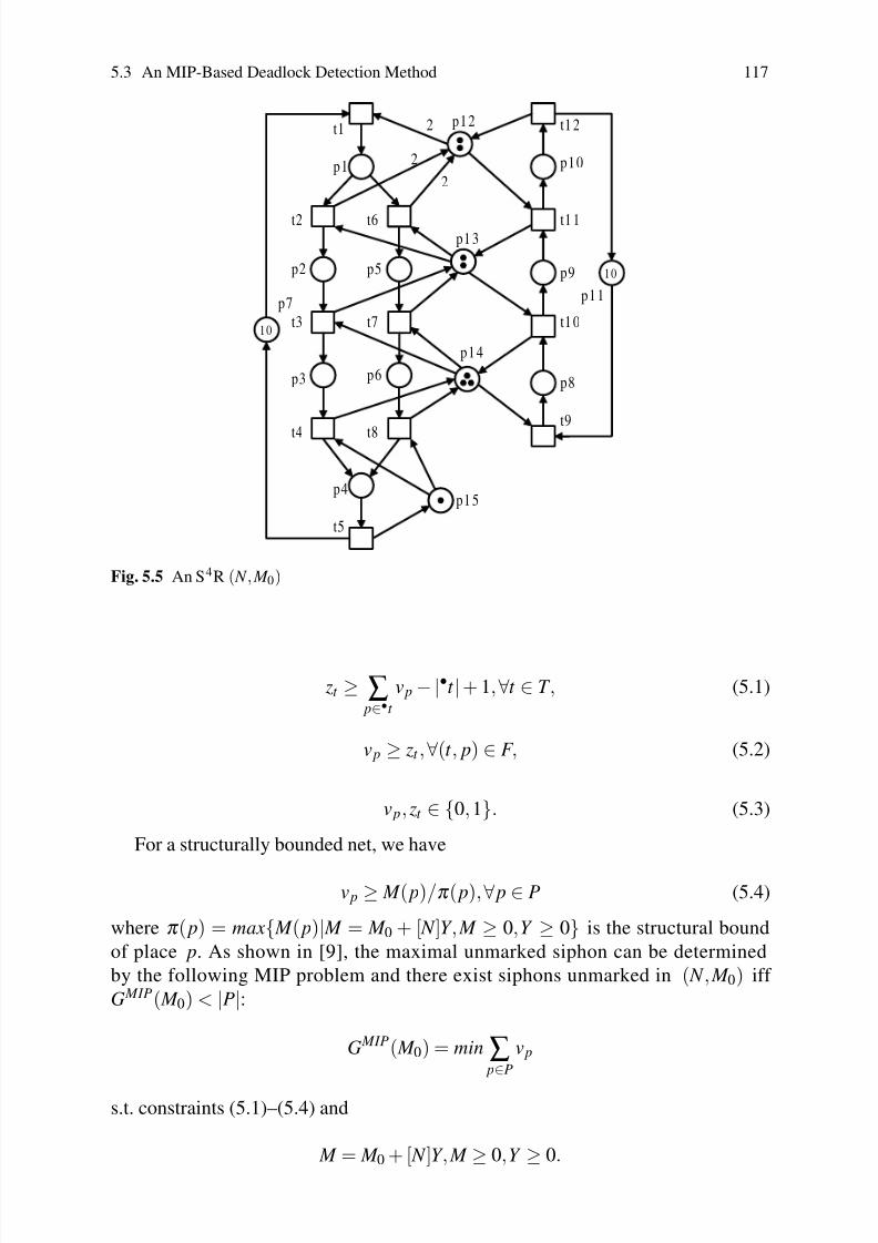
8/4/2019 Li Z., Zhou M. Deadlock Resolution in Automated Manufacturing Systems - A Novel Petri Net Approach
http://slidepdf.com/reader/full/li-z-zhou-m-deadlock-resolution-in-automated-manufacturing-systems-a-novel 131/249
5.3 An MIP-Based Deadlock Detection Method 117
p 1
t 1
t 2
t 3
t 4
t 5
t 6
t 7
t 8
p 2
p 3
p 4
p 5
p 6
p 7
t 1 2
t 1 1
t 1 0
p 1 0
p 9
t 9
p 8
p 1 1
p 1 5
p 1 22
2
2
p 1 3
p 1 4
1 0
1 0
Fig. 5.5 An S4R ( N , M 0)
zt ≥ ∑ p∈•t
v p −|•t |+ 1,∀t ∈ T , (5.1)
v p ≥ zt ,∀(t , p) ∈ F , (5.2)
v p, zt ∈ 0,1. (5.3)
For a structurally bounded net, we have
v p ≥ M ( p)/π ( p),∀ p ∈ P (5.4)
where π ( p) = max M ( p)| M = M 0 + [ N ]Y , M ≥ 0,Y ≥ 0 is the structural bound
of place p. As shown in [9], the maximal unmarked siphon can be determined
by the following MIP problem and there exist siphons unmarked in ( N , M 0) iff
G MIP( M 0) < |P|:
G MIP( M 0) = min∑ p∈P
v p
s.t. constraints (5.1)–(5.4) and
M = M 0 + [ N ]Y , M ≥ 0,Y ≥ 0.

8/4/2019 Li Z., Zhou M. Deadlock Resolution in Automated Manufacturing Systems - A Novel Petri Net Approach
http://slidepdf.com/reader/full/li-z-zhou-m-deadlock-resolution-in-automated-manufacturing-systems-a-novel 132/249
118 5 Deadlock Control Based on Elementary Siphons
Although an MIP problem is NP-hard, case studies in [9] show that its computa-
tional efficiency is relatively insensitive to the initial marking.
Theorem 5.5. Let ( N , M 0) be a Petri net with N = (P,T ,F ). There is no emptiable
siphon if G MIP( M 0) =|P
|.
Example 5.8. For the net in Fig. 2.7(a), its deadlock can be detected by solving the
following MIP problem:
MIN VP 1+ VP2+ VP 3+ VP 4+ VP5+ VP 6
SUBJECT TO
ZT 1-VP 1- VP 6≥-1 // ZTi denotes zt i
ZT 2-VP 2- VP 5≥-1 // VPi denotes v pi
ZT 3-VP 3- VP 6≥-1
ZT 4-VP 4
≥0
VP 1- ZT 4≥0VP 6- ZT 4≥0
VP 2- ZT 1≥0
VP 3- ZT 2≥0
VP 6- ZT 2≥0
VP 5- ZT 3≥0
VP 4- ZT 3≥0
2VP1-MP1≥0 // MPi denotes M ( pi)VP 2- MP2≥0
VP 3- MP3≥0VP 4- MP4≥0
VP 5- MP5≥0
VP 6- MP6≥0
MP 1+ Y1- Y4=2 // Yi denotes yi
MP 2- Y1+Y2=0
MP 3- Y2+Y3=0
MP 4- Y3+Y4=0
MP 5+ Y2- Y3=1
MP6+
Y1+
Y3-
Y2-
Y4= 1EN D
INT VP1
INT VP2
INT VP3
INT VP4
INT VP5
INT VP6
INT ZT1
INT ZT2
INT ZT3
INT ZT4
Note that the above source code follows the syntax of Lindo [38], where “int x”
indicates variable x ∈ 0,1. Lindo gives a feasible solution Z=2 with VP 2= VP 3= 1

8/4/2019 Li Z., Zhou M. Deadlock Resolution in Automated Manufacturing Systems - A Novel Petri Net Approach
http://slidepdf.com/reader/full/li-z-zhou-m-deadlock-resolution-in-automated-manufacturing-systems-a-novel 133/249

8/4/2019 Li Z., Zhou M. Deadlock Resolution in Automated Manufacturing Systems - A Novel Petri Net Approach
http://slidepdf.com/reader/full/li-z-zhou-m-deadlock-resolution-in-automated-manufacturing-systems-a-novel 134/249
120 5 Deadlock Control Based on Elementary Siphons
1. ∆+ : T → 2Π is a mapping defined as follows: If t ∈ T i, then ∆+(t ) = S ∈Π |t < N i
[S]i. If S ∈ ∆+(t ) then the set [S]i is reachable from t , i.e., there exists
a path in N i leading from t to an operation place p ∈ P Aithat is not included in S
but uses a resource of S, where [S] = ∪ni=1[S]i, P A = ∪n
i=1P Ai, and [S]i = [S]∩ P Ai
.
2. ∆− : T → 2Π
is a mapping defined as follows: If t ∈ T i, then ∆−(t ) = S ∈Π |[S]i < N i
t .
3. ∀i ∈ Nn, ∀S ∈Π , P iS = [S]i ∪ p ∈ P Ai
| p < N i[S]i, and PS = ∪n
i=1PiS.
Example 5.10. Take the net shown in Fig. 5.3 as an example. There are three
strict minimal siphons S1 = p5, p9, p12, p13, S2 = p4, p6, p13, p14, and S3 = p6, p9, p12, p13, p14. Their complementary sets are [S1] = p3, p4, [S2] = p5, p8,
and [S3] = p3, p4, p5, p8, respectively. We have downstream siphons ∆+(t 1) =∆+(t 2) = ∆+(t 8) =
S1,S2,S3
, ∆+(t 3) =
S2,S3
, and ∆+(t 4) = ∆+(t 10) = / 0.
Similarly, upstream siphons include ∆−(t 1) = ∆−(t 2) = ∆−(t 6) = ∆−(t 7) = / 0,∆−(t 3) = S1, and ∆−(t 4) = ∆−(t 5) = S1,S2,S3.
We have adjoint sets PS1= P1
S1∪P2
S1= ( p3 ∪ p7) ∪ ( p4 ∪ p8) =
p3, p4, p7, p8, PS2= P1
S2∪P2
S2= ( p5∪ p7, p3) ∪ p8 = p7, p3, p5, p8,
and PS3=P1
S3∪P2
S3= ( p3, p5∪ p7) ∪ p4, p8 = p7, p3, p5, p4, p8.
Definition 5.20. Let ( N , M 0) be an S3PR with N = ni=1 N i = (P A ∪ P0 ∪ P R,T ,F ).
The net ( N V , M 0V ) = (P A ∪ P0 ∪ P R ∪ PV ,T ,F ∪ F V , M 0V ) is the controlled system of
( N , M 0) iff:
1. PV = V S|S ∈ Π is a set of monitors such that there exists a bijective mapping
between Π and PV .
2. F V = F 1V ∪ F 2V ∪ F 3V , where
F 1V = (V S, t )|S ∈ ∆+(t ),t ∈ P0•,
F 2V = (t ,V S)|t ∈ [S]•,S /∈ ∆+(t ),
F 3V = ∪ni=1(t ,V S)|t ∈ T i \ P0•
,S /∈ ∆−(t ),• t ∩ P Ai⊆P i
S,t ≮ [S]i.
3. M 0V is defined as follows: (1) ∀ p ∈ P A ∪ P0 ∪ P R, M 0V ( p) = M 0( p) and (2) ∀V S ∈PV , M 0V (V S) = M 0(S) −1.
Theorem 5.6. ( N V , M 0V ) is live [16].
Example 5.11. For the net shown in Fig. 5.3, three monitors are needed to prevent
three strict minimal siphons from being emptied. We first take S1 = p5, p9, p12, p13as an example. Since P0 = p1, p10, we have P0•
= t 1,t 8. As a result, (V S1,t 1),
(V S1,t 8) ⊆ F 1V .
Due to [S1] = p3, p4, [S1]• = t 3,t 10. Note that S1 /∈ ∆+(t 3) and S1 /∈ ∆+(t 10).
We have (t 3,V S1),(t 10,V S1
) ⊆ F 2V .
Next let us find the arcs related to V S1 in F 3
V . LetT α = (T 1 \ P0•
) ∪ (T 2 \ P0•),
T β = t |S1 /∈ ∆−(t ),t ∈ T ,
T γ = t |•t ∩ P A1⊆P1
S ∪t |•t ∩ P A2⊆P2
S ,

8/4/2019 Li Z., Zhou M. Deadlock Resolution in Automated Manufacturing Systems - A Novel Petri Net Approach
http://slidepdf.com/reader/full/li-z-zhou-m-deadlock-resolution-in-automated-manufacturing-systems-a-novel 135/249
5.4 A Classical Deadlock Prevention Policy 121
T δ = t |t ≮ [S1]1∪t |t ≮ [S1]2.
We have
T α = t 2 − t 7,t 9 − t 11,
T β = t 1,t 2, t 6 − t 9,
T γ = t 2, t 3,t 6, t 9,t 10,T δ = t 3 − t 7,t 10, t 11.
It is easy to see that T α ∩ T β ∩ T γ ∩ T δ = t 6. Consequently, (t 6,V S1) ∈ F 3V .
For siphons S2 and S3, monitors V S2and V S3
can be added with (V S2,t 1), (V S2
,t 8),
(V S3,t 1), (V S3
,t 8) ⊆ F 1V , (t 4,V S2), (t 9,V S2
), (t 4,V S3), (t 10,V S3
) ⊆ F 2V , and (t 6,V S2),
(t 6,V S3) ⊆ F 3V . The controlled system for ( N , M 0) is shown in Fig. 5.6.
p 1
p 5
p 3
t 4
t 3
p 6
t 5
p 7
p 4
p 9
t 1 1
t 9
t 1 0
p 8
p 2
t 6
5
p 1 1
t 1
t 2
3p 1 0
p 1 5
p 1 4
p 1 3
p 1 2
t 8
t 7
t 6t 1
t 9t 8
VS 2
t 8
t 1
V S 1t 6
t 1 0t 3 t 1 0
t 8
t 1
V S 3t 6
t 4
Fig. 5.6 The controlled system of ( N , M 0)
According to Theorem 5.6, the net in Fig. 5.6 is live. ⊓⊔ Remark 5.1. For a strict minimal siphon S, this policy ensures that the maximal
number of tokens held by PS is not more than M 0(S). Since [S] ⊆PS, S cannot
be emptied if a monitor V S is added for it. For example, S1 = p5, p9, p12, p13 is
a strict minimal siphon with M 0(S1) = 2. Its monitor guarantees that the maximal
number of tokens held in PS1is M 0(S1) − 1 = 1.
Next we present an FMS example to illustrate the deadlock prevention policy.This FMS is extensively investigated in the literature [6, 7, 16, 24, 30–33, 52, 54].
Particularly, in a recent survey paper [36], this FMS is exploited as a benchmark
example to compare a variety of deadlock prevention policies in the literature.
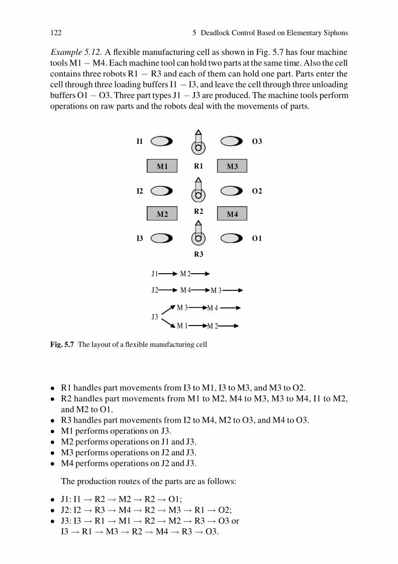
8/4/2019 Li Z., Zhou M. Deadlock Resolution in Automated Manufacturing Systems - A Novel Petri Net Approach
http://slidepdf.com/reader/full/li-z-zhou-m-deadlock-resolution-in-automated-manufacturing-systems-a-novel 136/249
122 5 Deadlock Control Based on Elementary Siphons
Example 5.12. A flexible manufacturing cell as shown in Fig. 5.7 has four machine
tools M1 − M4. Each machine tool can hold two parts at the same time. Also the cell
contains three robots R1 − R3 and each of them can hold one part. Parts enter the
cell through three loading buffers I1 − I3, and leave the cell through three unloading
buffers O1 − O3. Three part types J1 − J3 are produced. The machine tools performoperations on raw parts and the robots deal with the movements of parts.
M 1
M 2
M 3
M 4
R 1
R 2
R 3
I 1
I 2
I 3
O 3
O 2
O 1
J 1 M 2
J 2 M 4 M 3
J 3
M 3 M 4
M 1 M 2
Fig. 5.7 The layout of a flexible manufacturing cell
•R1 handles part movements from I3 to M1, I3 to M3, and M3 to O2.
• R2 handles part movements from M1 to M2, M4 to M3, M3 to M4, I1 to M2,and M2 to O1.
• R3 handles part movements from I2 to M4, M2 to O3, and M4 to O3.
• M1 performs operations on J3.
• M2 performs operations on J1 and J3.
• M3 performs operations on J2 and J3.
• M4 performs operations on J2 and J3.
The production routes of the parts are as follows:
• J1: I1 → R2 → M2 → R2 → O1;
• J2: I2 → R3 → M4 → R2 → M3 → R1 → O2;
• J3: I3 → R1 → M1 → R2 → M2 → R3 → O3 or
I3 → R1 → M3 → R2 → M4 → R3 → O3.

8/4/2019 Li Z., Zhou M. Deadlock Resolution in Automated Manufacturing Systems - A Novel Petri Net Approach
http://slidepdf.com/reader/full/li-z-zhou-m-deadlock-resolution-in-automated-manufacturing-systems-a-novel 137/249
5.4 A Classical Deadlock Prevention Policy 123
The flexible manufacturing cell contains global and local deadlocks if it is not
properly supervised. Suppose that the system is in the scenario that M4 is fully
occupied by machining two J3-type raw parts and R3 picks up a J2-type raw part
and tries to upload M4. The processes to produce J2 and J3 remain indefinitely
blocked since no further operations on them can be performed. That is to say, thesystem is in a local deadlock state.
While, if the system is in such a state that M4 is fully occupied by machining
two J3-type raw parts, R3 has picked up a J2-type raw part from I2 and is trying to
upload M4, M2 is fully occupied by machining two J1-type raw parts, and R2 has
downloaded a J3-type part from M1 and is trying to upload M2, it will enter a global
deadlock state. In this case, the whole system will be completely blocked.
The system can be modeled with Petri nets. Its model ( N , M 0) is shown in Fig.
5.8. The physical meaning of each place is explained in Table 5.1. Let T 1 = t 11 −t
14, T
2=
t
15 −t
20, and T
3=
t
1 −t
10. This model belongs to S3PR where p
1,
p5, and p14 are idle process places, p20 − p26 are resource places, and the others are
operation places. The occurrence of system deadlocks corresponds to the existence
of unmarked siphons in the model. They can be successfully prevented by properly
supervising the siphons in their net model.
There are 18 strict minimal siphons in the Petri net model of the flexible man-
ufacturing cell. These siphons, their complementary sets, and their corresponding
monitors are shown in Tables 5.2 − 5.4, respectively.
Next S1 = p10, p18, p22, p26, S3 = p2, p4, p8, p13, p17, p21, p26, and S5 =
p2, p4, p8, p10, p17, p21, p22, p26
are taken as examples to show the way of adding
monitors to prevent them from being unmarked.
According to the definition of the complementary set of a siphon, we have
[S1] = ( H ( p22) ∪ H ( p26)) \ S1 = ( p10, p19∪ p13, p18) \ S1 = p13, p19, [S3] =( p2, p4, p8, p12, p17 ∪ p13, p18) \ S3 = p12, p18, and [S5] =( p2, p4, p8, p12,
p17∪ p10, p19∪ p13, p18)\S5 = p12, p13, p18, p19.
Since P0 = p1, p5, p14, we have P0•= t 1,t 11,t 15. S1,S3,S5 ⊆ ∆+(t 1),
S1,S3,S5 ⊆ ∆+(t 15), and ∀S ∈ S1,S3,S5, S /∈ ∆+(t 11). This leads to (V S1,t 1),
(V S1,t 15), (V S3
,t 1), (V S3,t 15),(V S5
,t 1),(V S5,t 15) ⊆ F 1V .
From [S1] =
p13, p19
, [S1]• =
t 10, t 16
. It is clear that S1 /
∈∆+(t 10) and
S1 /∈∆+(t 16). Therefore, (t 10,V S1 ),(t 16,V S1 ) ⊆ F 2V . From [S3] = p12, p18, [S3]• =t 9,t 17. It is clear that S3 /∈∆+(t 9) and S3 /∈∆+(t 17). Therefore, (t 9,V S3
), (t 17,V S3)
⊆ F 2V .
The case of S5 is slightly different from S1 and S3. From [S5] = p12, p13, p18,
p19, we have [S5]• = t 9,t 10,t 16,t 17. However, S5 ∈ ∆+(t 9), S5 ∈ ∆+(t 16), S5 /∈∆+(t 10), and S5 /∈ ∆+(t 17). As a result, (t 10,V S5
),(t 17,V S5) ⊆ F 2V .
In order to determine the set of additional arcs in F 3V for V S1, V S3
, and V S5, we first
find PS1, PS3
, and PS5.
PS1=P1
S1
∪P2
S1
∪P3
S1, where P i
S1= [S1]i
∪ p
∈P Ai
| p < N i
[S1]i
, i = 1,2,3.
It is easy to see that [S1]1 = / 0, [S1]2 = p19, [S1]3 = p13, p ∈ P A1 | p < N 1 [S1]1 = / 0, p ∈ P A2
| p < N 2[S1]2 = / 0, and p ∈ P A3
| p < N 3[S1]3 = p6, p11, p12. Hence
PS1= p13, p19, p6, p11, p12.
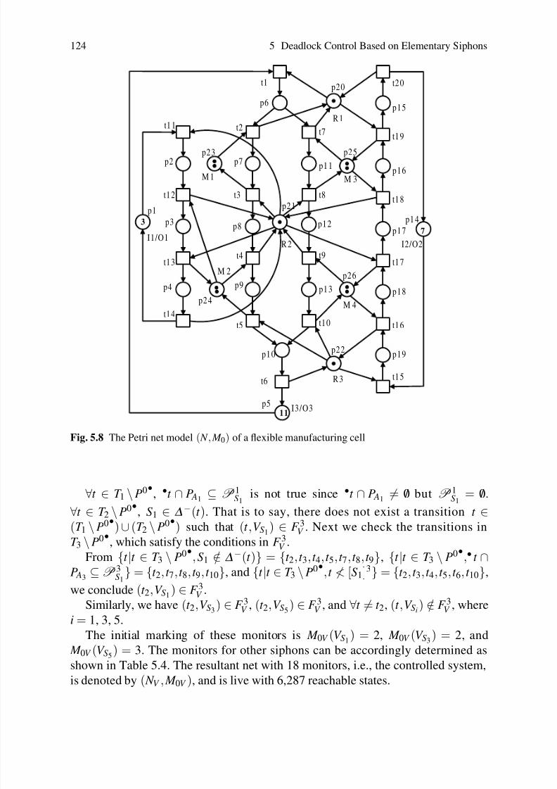
8/4/2019 Li Z., Zhou M. Deadlock Resolution in Automated Manufacturing Systems - A Novel Petri Net Approach
http://slidepdf.com/reader/full/li-z-zhou-m-deadlock-resolution-in-automated-manufacturing-systems-a-novel 138/249
124 5 Deadlock Control Based on Elementary Siphons
p 6
t 1
t 2
t 3
t 4
t 7
t 8
t 9
p 7
p 8
p 1 1
p 1 2
t 5 t 1 0
p 9 p 1 3
t 6
p 5
t 1 1
t 1 2
t 1 3
p 2
p 3
p 4
t 1 4
t 2 0
t 1 9
t 1 8
p 1 5
p 1 6
p 1 7
t 1 7
t 1 6
p 1 8
p 1 9
t 1 5
p 1 4
I 2 / O 2
p 2 0
R 1
p 1
I 1 / O 1
p 1 0
p 2 1
R 2
p 2 2
R 3
p 2 3
M 1
p 2 4
M 2
p 2 5
M 3
p 2 6
M 4
I 3 / O 3
3
1 1
7
Fig. 5.8 The Petri net model ( N , M 0) of a flexible manufacturing cell
∀t ∈ T 1 \ P0•, •t ∩ P A1
⊆ P1S1
is not true since •t ∩ P A1= / 0 but P1
S1= / 0.
∀t ∈ T 2 \ P0•, S1 ∈ ∆−(t ). That is to say, there does not exist a transition t ∈
(T 1 \ P0•) ∪ (T 2 \ P0•
) such that (t ,V S1) ∈ F 3V . Next we check the transitions in
T 3
\P0•
, which satisfy the conditions in F 3V .
From t |t ∈ T 3 \ P0•,S1 /∈ ∆−(t ) = t 2,t 3,t 4,t 5,t 7,t 8,t 9, t |t ∈ T 3 \ P0•,• t ∩P A3
⊆P3S1
= t 2, t 7,t 8, t 9,t 10, and t |t ∈ T 3 \ P0•,t ≮ [S1]3 = t 2, t 3,t 4, t 5,t 6, t 10,
we conclude (t 2,V S1) ∈ F 3V .
Similarly, we have (t 2,V S3) ∈ F 3V , (t 2,V S5
) ∈ F 3V , and ∀t = t 2, (t ,V Si) /∈ F 3V , where
i = 1, 3, 5.
The initial marking of these monitors is M 0V (V S1) = 2, M 0V (V S3
) = 2, and
M 0V (V S5) = 3. The monitors for other siphons can be accordingly determined as
shown in Table 5.4. The resultant net with 18 monitors, i.e., the controlled system,
is denoted by ( N V , M 0V ), and is live with 6,287 reachable states.

8/4/2019 Li Z., Zhou M. Deadlock Resolution in Automated Manufacturing Systems - A Novel Petri Net Approach
http://slidepdf.com/reader/full/li-z-zhou-m-deadlock-resolution-in-automated-manufacturing-systems-a-novel 139/249
5.5 An Elementary Siphon-Based Deadlock Prevention Policy 125
Table 5.1 Meanings of the places in the net model shown in Fig. 5.8
p1: Raw materials in I1 available
p2: R2 uploads M2
p3: M2 machining
p4: R2 downloads M2 and puts finished parts in O1
p5: Raw materials in I3 available p6: R1 uploads M1 or M3
p7: M1 machining
p8: R2 downloads M1 and uploads M2
p9: M2 machining
p10: R3 downloads M2 or M4 and put finished parts in O3
p11: M3 machining
p12: R2 downloads M3 and uploads M4
p13: M4 machining
p14: Raw materials in I2 available
p15: R1 downloads M3 and puts finished parts in O2
p16: M3 machining p17: R2 downloads M4 and uploads M3
p18: M4 machining
p19: R3 uploads M4
p20: R1 available
p21: R2 available
p22: R3 available
p23: M1 available
p24: M2 available
p25: M3 available
p26: M4 available
Table 5.2 Strict minimal siphons in the model ( N , M 0), where * means the corresponding siphons
are dependent ones
S Places S Places
S1 p10, p18, p22, p26 S2 p4, p9, p12, p17, p21, p24
S3 p2, p4, p8, p13, p17, p21, p26 S4 p2, p4, p8, p12, p16, p21, p25
S∗5 p2, p4, p8, p10, p17, p21, p22, p26 S∗
6 p4, p9, p12, p16, p21, p24, p25
S∗7 p4, p9, p13, p17, p21, p24, p26 S∗
8 p2, p4, p8, p13, p16, p21, p25, p26
S9 p4, p10, p17, p21, p22, p24, p26 S∗10 p4, p9, p13, p16, p21, p24, p25, p26
S∗11 p2, p4, p8, p10, p16, p21, p22, p25, p26 S12 p2, p4, p8, p12, p15, p20, p21, p23, p25
S∗13 p4, p10, p16, p21, p22, p24, p25, p26 S∗
14 p4, p9, p12, p15, p20, p21, p23, p24, p25
S∗15 p2, p4, p8, p13, p15, p20, p21, p23, p25, p26 S∗
16 p4, p9, p13, p15, p20, p21, p23− p26
S∗17 p2, p4, p8, p10, p15, p20− p23, p25, p26 S∗
18 p4, p10, p15, p20− p26
5.5 An Elementary Siphon-Based Deadlock Prevention Policy
The policy proposed in [16] indicates that the number of additional monitors equals
that of strict minimal siphons in an S3PR. That is to say, the size of the resultant
liveness-enforcing supervisor is in theory exponential with respect to the plant netsize since the number of strict minimal siphons grows in a general case exponen-
tially with respect to the net size. It implies that the supervisor is much more struc-
turally complex than the plant model originally built.

8/4/2019 Li Z., Zhou M. Deadlock Resolution in Automated Manufacturing Systems - A Novel Petri Net Approach
http://slidepdf.com/reader/full/li-z-zhou-m-deadlock-resolution-in-automated-manufacturing-systems-a-novel 140/249
126 5 Deadlock Control Based on Elementary Siphons
Table 5.3 The complementary sets of the strict minimal siphons
[S] Places [S] Places
[S1] p13, p19 [S2] p2, p3, p8
[S3] p12, p18 [S4] p11, p17
[S5] p12, p13, p18, p19 [S6] p2, p3, p8, p11, p17
[S7] p2, p3, p8, p12, p18 [S8] p11, p12, p17, p18
[S9] p2, p3, p8, p9, p12, p13, p18, p19 [S10] p2, p3, p8, p11, p12, p17, p18
[S11] p11, p12, p13, p17, p18, p19 [S12] p6, p7, p11, p16, p17
[S13] p2, p3, p8, p9, p11, p12, p13, p17− p19 [S14] p2, p3, p6, p7, p8, p11, p16, p17
[S15] p6, p7, p11, p12, p16, p17, p18 [S16] p2, p3, p6, p7, p8, p11, p12, p16, p17, p18
[S17] p6, p7, p11, p12, p13, p16− p19 [S18] p2, p3, p6, p7, p8, p9, p11− p13, p16− p19
Table 5.4 Monitors for the model ( N , M 0)
Monitor M 0V (·) Preset Postset Monitor M 0V (·) Preset Postset
V S1
2 t 2, t 10,t 16 t 1,t 15 V S2
2 t 4,t 7,t 13 t 1, t 11
V S32 t 2, t 9, t 17 t 1,t 15 V S4
2 t 2,t 8,t 18 t 1, t 15
V S53 t 2, t 10,t 17 t 1,t 15 V S6
4 t 4,t 8,t 13,t 18 t 1, t 11, t 15
V S74 t 4, t 9, t 13,t 17 t 1,t 11, t 15 V S8
4 t 2,t 9,t 18 t 1, t 15
V S95 t 5, t 10,t 13,t 17 t 1,t 11, t 15 V S10
6 t 4,t 9,t 13,t 18 t 1, t 11, t 15
V S115 t 2, t 10,t 18 t 1,t 15 V S12
5 t 3,t 8,t 19 t 1, t 15
V S137 t 5, t 10,t 13,t 18 t 1,t 11, t 15 V S14
7 t 4,t 8,t 13,t 19 t 1, t 11, t 15
V S157 t 3, t 9, t 19 t 1,t 15 V S16
9 t 4,t 9,t 13,t 19 t 1, t 11, t 15
V S178 t 3, t 10,t 19 t 1,t 15 V S18
10 t 5,t 10,t 13, t 19 t 1, t 11, t 15
Motivated by the need to reduce the structural complexity of the liveness-
enforcing supervisor resulting from the policy in [16], the concept of elementary
siphons is developed in [30]. This section presents an improved deadlock preven-
tion policy for an S3PR, which is based on the concept of elementary siphons. First
strict minimal siphons are divided into elementary and dependent ones. Monitors
are added for the elementary siphons only and the controllability of a dependent
siphon is ensured by properly supervising its elementary siphons. If a dependent
siphon cannot be implicitly controlled by using the monitors for elementary siphons
only, a monitor is added for it.
In the deadlock prevention policy in [16], the addition of monitor V S puts itscorresponding siphon S under control. In what follows, ( N V , M 0V ) is used to denote
a controlled system for a plant S3PR ( N , M 0).
Lemma 5.1. Let S and V S be a siphon and its corresponding monitor, respectively.
Then ∀ M ∈ R( N V , M 0V ) , the following invariant relation holds:
M (V S) +n
∑i=1
M (P iS) = M 0V (V S).
Consider ∪ni=1P
iS =PS and ∀i = j,P i
S ∩P jS = / 0, the token invariant relation in
Lemma 5.1 can be rewritten as M (V S) + M (PS) = M 0V (V S). It is the token invariant

8/4/2019 Li Z., Zhou M. Deadlock Resolution in Automated Manufacturing Systems - A Novel Petri Net Approach
http://slidepdf.com/reader/full/li-z-zhou-m-deadlock-resolution-in-automated-manufacturing-systems-a-novel 141/249
5.5 An Elementary Siphon-Based Deadlock Prevention Policy 127
relation that ensures the controllability of a strict minimal siphon such that it can
never be emptied under any reachable marking in ( N V , M 0V ).
Example 5.13. In Example 5.12, V S1is the monitor for S1 = p10, p18, p22, p26 with
M 0V (V S1) = 2 and PS1
=
p13, p19, p6, p11, p12
. Lemma 5.1 indicates that
∀ M
∈ R( N V , M 0V ), M (V S) + M ( p13) + M ( p19) + M ( p6) + M ( p11) + M ( p12) = 2. Hence,
the maximal number of tokens staying at [S1] = p13, p19 is not greater than 2, i.e.,
∀ M ∈ R( N V , M 0V ), M ( p13) + M ( p19) ≤ 2.
Recall the meanings of the complementary set of a siphon in an S3PR, which
contains operation places only. The places in a complementary set compete for re-
sources with the operation places in a siphon. When the complementary set holds
all the tokens initially marked in a siphon, the siphon is emptied and remains so for-
ever, leading to occurrences of dead transitions. On the contrary, if at any reachable
marking the maximal number of tokens held by the places in the complementary set
is not greater than the number of tokens initially marked in it, the siphon can neverbe emptied.
For siphon S1 = p10, p18, p22, p26 with M 0V (S1) = M 0(S1) = 3 and [S1] = p13, p19, we conclude that S1 can never be emptied due to the addition of mon-
itor V S1that keeps M ( p13) + M ( p19) ≤ 2, ∀ M ∈ R( N V , M 0V ). It is easy to see that
min M (S1)| M ∈ R( N V , M 0V ) = M 0(S1) − M 0V (V S1) = 1.
Proposition 5.1. Let V S be a monitor for siphon S in ( N V , M 0V ). Then V S +∑ p∈PSp
is a P-semiflow of N V .
Proof. Let I denote P-vector V S +∑ p∈PSp. We need to show I T [ N V ] = 0T . I T [ N V ] =
[ N V ](V S, ·) +∑ p∈PS[ N V ]( p, ·) = [ N V ](V S, ·) + [ N V ](PS, ·) = [ N V ](V S, ·) +∑n
i=1[ N V ]
(P iS, ·), where n is the number of subnets by which the plant S3PR ( N , M 0) is com-
posed.
Since P iS is a subset of places in state machine N i, ∀t ∈ T i, [ N ](P i
S,t ) =[ N V ](P
iS, t ) is −1, 0, or 1. Note that ∀i, j ∈ Nn(i = j), T i ∩ T j = / 0. We have ∀t ∈ T ,
[ N V ](PS,t ) is −1, 0, or 1.
By the way of adding monitors in Definition 5.20, ∀t ∈ T , [ N V ](PS,t ) = 1 im-
plies [ N V ](V S,t ) =−
1 and [ N V ](PS,t ) =−
1 implies [ N V ](V S,t ) = 1. Therefore,
∀t ∈ T , [ N V ](V S,t ) + [ N V ](PS,t ) = 0, indicating that I T [ N V ] = 0T . We conclude
that V S +∑ p∈PSp is a P-semiflow of N V . ⊓⊔
Next, for a siphon S, a parameter ξS, called the control depth variable of the
siphon, is introduced in order to establish a method to ensure the controllability of
a dependent siphon by properly supervising its elementary ones.
Proposition 5.2. Let V S be a monitor computed by Definition 5.20 for a siphon
S in an S3PR ( N , M 0). S is controlled if M 0V (V S) = M 0(S) − ξS where 1 ≤ ξS ≤ M 0(S) − 1.
Proof. By Lemma 5.1, ∀ M ∈ R( N V , M 0V ), M (V S) + M (PS) = M 0V (V S), where
PS = ∪ni=1P
iS.

8/4/2019 Li Z., Zhou M. Deadlock Resolution in Automated Manufacturing Systems - A Novel Petri Net Approach
http://slidepdf.com/reader/full/li-z-zhou-m-deadlock-resolution-in-automated-manufacturing-systems-a-novel 142/249
128 5 Deadlock Control Based on Elementary Siphons
M (PS) = M 0(S) −ξS − M (V S).
Since M (V S) ≥ 0, M (PS) ≤ M 0(S) −ξS is true. By [S] ⊆PS, we have
M ([S]) ≤ M 0(S) −ξS. (5.5)
According to the definition of the complementary set of a siphon, [S] ∪ S is the
support of a P-semiflow of N . It is also a P-semiflow of N V . Consequently, ∀ M ∈ R( N V , M 0V ), M ([S]) + M (S) = M 0(S) = M 0V (S), leading to the truth of
M (S) = M 0(S) − M ([S]). (5.6)
Consider (5.5) and (5.6); M (S) ≥ M 0(S) − ( M 0(S)−ξS), i.e.,
M (S) ≥ ξS ≥ 1.
This implies that at any reachable marking in R( N V , M 0V ), S can never be un-
marked. ⊓⊔Increasing ξS intends to tighten the control of siphon S, which may degrade the
control performance from the behavior permissiveness point of view. Specifically,
a large ξS implies that some good (safe) states are possibly removed from the con-
trolled system.
Corollary 5.1. Let S be a siphon in an S3PR and V S be its monitor defined in Propo-sition 5.2. In ( N V , M 0V ) , M min(S) = ξS.
The relation between the controllability of elementary siphons and that of depen-
dent ones can be established by means of the results in Chap. 3. To demonstrate this,
let us first consider the Petri net in Fig. 5.3. There are three strict minimal siphons:
S1 = p5, p9, p12, p13, S2 = p4, p6, p13, p14, and S3 = p6, p9, p12, p13, p14. It
is verified that the rank of its characteristic T -vector matrix of these siphons equals
two, indicating that there are two elementary siphons. The third one is dependent
withηS3 = ηS1 +ηS2
if S1
and S2
are selected to be elementary ones. In other words,
Π E = S1,S2 implies Π D = S3.
Suppose that V S1and V S2
are added for S1 and S2 with control depth variables ξS1
and ξS2, respectively. Let ( N V , M 0V ) denote the resultant net with V S1
and V S2. We
then check the controllability of S3 in ( N V , M 0V ). According to Corollary 3.5, S3 is
controlled if
M 0V (S3) > M 0V (S1) + M 0V (S2) − M min(S1)− M min(S2).
i.e.,
M 0V (S3) > M 0V (S1) + M 0V (S2) −ξS1−ξS2
.
It is easy to see that M 0V (S1) = M 0(S1) = 2, M 0V (S2) = M 0(S2) = 2, and
M 0V (S3) = M 0(S3) = 3. The controllability condition is true if ξS1= ξS2
= 1. This
Hence, we have
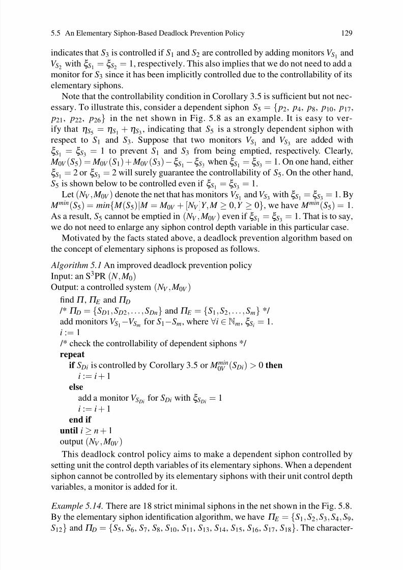
8/4/2019 Li Z., Zhou M. Deadlock Resolution in Automated Manufacturing Systems - A Novel Petri Net Approach
http://slidepdf.com/reader/full/li-z-zhou-m-deadlock-resolution-in-automated-manufacturing-systems-a-novel 143/249
5.5 An Elementary Siphon-Based Deadlock Prevention Policy 129
indicates that S3 is controlled if S1 and S2 are controlled by adding monitors V S1and
V S2with ξS1
= ξS2= 1, respectively. This also implies that we do not need to add a
monitor for S3 since it has been implicitly controlled due to the controllability of its
elementary siphons.
Note that the controllability condition in Corollary 3.5 is sufficient but not nec-essary. To illustrate this, consider a dependent siphon S5 = p2, p4, p8, p10, p17,
p21, p22, p26 in the net shown in Fig. 5.8 as an example. It is easy to ver-
ify that ηS5= ηS1
+ ηS3, indicating that S5 is a strongly dependent siphon with
respect to S1 and S3. Suppose that two monitors V S1and V S3
are added with
ξS1= ξS3
= 1 to prevent S1 and S3 from being emptied, respectively. Clearly,
M 0V (S5) = M 0V (S1) + M 0V (S3)−ξS1−ξS3
when ξS1= ξS3
= 1. On one hand, either
ξS1= 2 or ξS3
= 2 will surely guarantee the controllability of S5. On the other hand,
S5 is shown below to be controlled even if ξS1= ξS3
= 1.
Let ( N V , M 0
V ) denote the net that has monitors V S1
and V S3
with ξS1
= ξS3
= 1. By
M min(S5) = min M (S5)| M = M 0V + [ N V ]Y , M ≥ 0,Y ≥ 0, we have M min(S5) = 1.
As a result, S5 cannot be emptied in ( N V , M 0V ) even if ξS1= ξS3
= 1. That is to say,
we do not need to enlarge any siphon control depth variable in this particular case.
Motivated by the facts stated above, a deadlock prevention algorithm based on
the concept of elementary siphons is proposed as follows.
Algorithm 5.1 An improved deadlock prevention policy
Input: an S3PR ( N , M 0)Output: a controlled system ( N V , M 0V )
find Π , Π E and Π D /* Π D = S D1,S D2, . . . ,S Dn and Π E = S1,S2, . . . ,Sm */
add monitors V S1−V Sm for S1−Sm, where ∀i ∈ Nm, ξSi
= 1.
i := 1
/* check the controllability of dependent siphons */
repeat
if S Di is controlled by Corollary 3.5 or M min0V (S Di) > 0 then
i := i + 1
else
add a monitor V S Di for S Di with ξS Di = 1i := i + 1
end if
until i ≥ n + 1
output ( N V , M 0V )
This deadlock control policy aims to make a dependent siphon controlled by
setting unit the control depth variables of its elementary siphons. When a dependent
siphon cannot be controlled by its elementary siphons with their unit control depth
variables, a monitor is added for it.
Example 5.14. There are 18 strict minimal siphons in the net shown in the Fig. 5.8.
By the elementary siphon identification algorithm, we have Π E = S1,S2,S3,S4,S9,
S12 and Π D = S5, S6, S7, S8, S10, S11, S13, S14, S15, S16, S17, S18. The character-

8/4/2019 Li Z., Zhou M. Deadlock Resolution in Automated Manufacturing Systems - A Novel Petri Net Approach
http://slidepdf.com/reader/full/li-z-zhou-m-deadlock-resolution-in-automated-manufacturing-systems-a-novel 144/249
130 5 Deadlock Control Based on Elementary Siphons
istic T -vector relation between elementary and dependent siphons is shown in Table
5.5.
Table 5.5 The characteristic T -vector relation between dependent and elementary siphons
S∗ η relationship S∗ η relationship
S5 ηS5= ηS1
+ηS3S6 ηS6
= ηS2+ηS4
S7 ηS7= ηS2
+ηS3S8 ηS8
= ηS3+ηS4
S10 ηS10= ηS2
+ηS3+ηS4
S11 ηS11= ηS1
+ηS3+ηS4
S13 ηS13= ηS4
+ηS9S14 ηS14
= ηS2+ηS12
S15 ηS15= ηS3
+ηS12S16 ηS16
= ηS2+ηS3
+ηS12
S17 ηS17= ηS1
+ηS3+ηS12
S18 ηS18= ηS9
+ηS12
The controllability of siphon S6 depends on whether M 0(S6)> M 0(S2)+ M 0(S4)
−ξS2 −ξS4 is true. Since M 0(S6) = 5, M 0(S2) = 3, and M 0(S4) = 3, S6 is controlled if monitors V S2
and V S4are added when ξS2
= ξS4= 1.
The controllability of S16 depends on the truth of M 0(S16) > M 0(S2) + M 0(S3) + M 0(S12)−ξS2
−ξS3−ξS12
. By M 0(S16) = 10, M 0(S2) = 3, M 0(S3) = 3, and M 0(S12) =6, this inequality holds when ξS2
= ξS3= ξS12
= 1.
By Algorithm 5.1, it is easy to see that all dependent siphons are controlled by
adding six monitors for the elementary siphons only with each siphon control depth
variable being unit. That is to say, the addition of six monitors leads to a liveness-
enforcing supervisor for the Petri net model of the FMS. Furthermore, the supervisor
results in the same permissive behavior with the one due to the deadlock preventionpolicy in [16].
The number of monitors resulting from Algorithm 5.1 may be greater than that
of elementary siphons. When the inequality concerning the controllability of a de-
pendent siphon is not true, or it is not controlled by solving the corresponding LPP,
a monitor needs to be added for it. As a result, the number of monitors resulting
from Algorithm 5.1 is in theory exponential with respect to the net size.
A natural and fascinating problem is to find a liveness-enforcing supervisor with
monitors that are added for elementary siphons only. The control of a dependentsiphon is ensured by properly setting the control depth variables of its elementary
siphons. If this is achieved, the size of the resulting controlled system is limited to
2n, where n is the size of the plant Petri net model.
Theorem 5.7. Let ( N , M 0) be an S3PR and ( N V , M 0V ) be the net resulting from
adding monitors for m elementary siphons only by Definition 5.20. ( N V , M 0V ) is
a controlled system with m monitors if the following LPP has a feasible solution:
minm
∑i=1
ξSi
s.t.

8/4/2019 Li Z., Zhou M. Deadlock Resolution in Automated Manufacturing Systems - A Novel Petri Net Approach
http://slidepdf.com/reader/full/li-z-zhou-m-deadlock-resolution-in-automated-manufacturing-systems-a-novel 145/249
5.5 An Elementary Siphon-Based Deadlock Prevention Policy 131
M 0(S D j) >m
∑i=1
ai( M 0(Si) −ξSi), j = 1,2, . . . ,n,
1 ≤ ξSi ≤ M 0(Si) −1, i = 1,2, . . . ,m,
where Π D = S D j| j = 1,2, . . . ,n and Π E = Si|i = 1,2, . . . ,m.
Proof. If the LPP has a feasible solution, it means that all dependent siphons are
controlled by properly setting the control depth variables of the elementary siphons.
Furthermore, the elementary siphons can be controlled by the monitors. As a result,
( N V , M 0V ) is a controlled system with liveness. ⊓⊔ Example 5.15. For the Petri net shown in Fig. 5.8, monitors V S1
−V S4, V S9
, and V S12
are added. By solving the following LPP:
z = min4
∑i=1
ξSi+ξS9
+ξS12
s.t.
M 0(S5) > M 0(S1) + M 0(S3) −ξS1−ξS3
,
M 0(S6) > M 0(S2) + M 0(S4) −ξS2−ξS4
,
M 0(S7) > M 0(S2) + M 0(S3) −ξS2−ξS3
,
M 0
(S8
) > M 0
(S3
) + M 0
(S4
)−ξ
S3 −ξ
S4
,
M 0(S10) > M 0(S2) + M 0(S3) + M 0(S4) −ξS2−ξS3
−ξS4,
M 0(S11) > M 0(S1) + M 0(S3) + M 0(S4) −ξS1−ξS3
−ξS4,
M 0(S13) > M 0(S4) + M 0(S9) −ξS4−ξS9
,
M 0(S14) > M 0(S2) + M 0(S12) −ξS2−ξS12
,
M 0(S15) > M 0(S3) + M 0(S12) −ξS3−ξS12
,
M 0(S16) > M 0(S2) + M 0(S3) + M 0(S12)−ξS2−ξS3
−ξS12,
M 0(S17) > M 0(S1) + M 0(S3) + M 0(S12)−ξS1−ξS3
−ξS12,
M 0(S18) > M 0(S9) + M 0(S12) −ξS9−ξS12
,
1
≤ξS1
≤ M 0(S1)
−1,
1 ≤ ξS2 ≤ M 0(S2) − 1,
1 ≤ ξS3≤ M 0(S3) − 1,
1 ≤ ξS4≤ M 0(S4) − 1,
1 ≤ ξS9≤ M 0(S9) − 1,
1 ≤ ξS12≤ M 0(S12) −1.
an optimal solution z∗ = 7 with ξS1= 2, ξS2
= 1, ξS3= 1, ξS4
= 1, ξS9= 1, and ξS12
=1 is found. This leads to M 0V (V S1
) = 1, M 0V (V S2) = 2, M 0V (V S3
) = 2, M 0V (V S4) = 2,
M 0V (V S9) = 5, and M 0V (V S12
) = 5. However, the obtained supervisor may be more
restrictive than the one in Example 5.12 due to a larger control depth variable of S1.
Specially, the number of reachable states of the controlled system in Example 5.12
is 6,287 and that in this example leads to 3,506 reachable states only.

8/4/2019 Li Z., Zhou M. Deadlock Resolution in Automated Manufacturing Systems - A Novel Petri Net Approach
http://slidepdf.com/reader/full/li-z-zhou-m-deadlock-resolution-in-automated-manufacturing-systems-a-novel 146/249
132 5 Deadlock Control Based on Elementary Siphons
5.6 An MIP-Based Deadlock Prevention Policy
The deadlock prevention policies in [16] and in Sect. 5.5 depend on the complete
siphon enumeration of a plant Petri net model. Its computation is expensive since
the number of siphons grows fast with respect to the net size. For example, INA[49], a popular Petri net analysis tool, is used to find all minimal siphons in a net
with 72 places and 64 transitions, the computation in a personal computer aborts
due to memory overflow after several days [33]. This section introduces a deadlock
prevention policy that combines the concept of elementary siphons and MIP-based
deadlock detection method. More importantly, the complete siphon enumeration
is avoided, leading to better computational efficiency. The following results play
an important role in the establishment of the efficient deadlock prevention policy
in [33].
Proposition 5.3. Let ( N V , M 0V ) be the net resulting from adding monitors for siphons
to an S3PR ( N , M 0) by the approach in [16]. Then ( N V , M 0V ) is an ES3PR.
Corollary 5.2. An ES3PR ( N V , M 0V ) is live iff no siphon in it can become empty.
Corollary 5.3. An ES3PR ( N V , M 0V ) is live iff G MIP( M 0V ) = |P A ∪ P0 ∪ P R ∪ PV | ,where PV is the set of monitors.
The idea underlying the deadlock prevention policy presented in this section pro-
ceeds in an iterative way that can be stated as follows. First, the MIP-based dead-
lock detection method is applied to a plant S3
PR net model ( N , M 0). If no unmarkedsiphon can be derived, it indicates that ( N , M 0) itself is live since no siphon can be-
come empty. If not, an unmarked maximal siphon S∗ is hence obtained. By using
the minimal siphon extraction approach in [34], a minimal siphon S1 from S∗ is then
derived. Let Π = S1.
The MIP-based method is applied to ( N , M 0) with a constraint M ([S1]) ≤ M 0(S1)−1, ∀ M ∈ R( N , M 0). If no unmarked maximal siphon can be found, S1 is the only
siphon that can be emptied in ( N , M 0). It is then controlled by adding monitor V S1
according to Definition 5.20 and the resultant net ( N V , M 0V ) is live. Otherwise, we
derive a strict minimal siphon S2 and Π is updated by putting S2 into it. Accordingly,a constraint M ([S2]) ≤ M 0(S2) −1 is generated for the next iteration.
Suppose that at some step, a minimal siphon Si is found. We have Π = S1,
S2, . . ., Si and constraint M ([Si]) ≤ M 0(Si) − 1. The MIP-based deadlock detec-
tion method is applied again to ( N , M 0) with constraints M ([S1]) ≤ M 0(S1) − 1,
M ([S2]) ≤ M 0(S2) −1, . . ., and M ([Si]) ≤ M 0(Si) −1. This process proceeds until no
unmarked siphon can be found and a set of minimal siphons Π is finally obtained.
With the set of siphons Π , Algorithm 5.1 can be used to compute the monitors of
the supervisor for ( N , M 0). Note that in general, Π computed in this way is not nec-
essarily the set of all strict minimal siphons in ( N , M 0). Even if Π happens to be the
set of all strict minimal siphons in ( N , M 0), it can be computed efficiently through
the MIP-based deadlock detection and minimal siphon extraction method, particu-
larly, when a large net model is dealt with. We summarize the deadlock detection
and siphon extraction algorithm as follows.

8/4/2019 Li Z., Zhou M. Deadlock Resolution in Automated Manufacturing Systems - A Novel Petri Net Approach
http://slidepdf.com/reader/full/li-z-zhou-m-deadlock-resolution-in-automated-manufacturing-systems-a-novel 147/249
5.6 An MIP-Based Deadlock Prevention Policy 133
Algorithm 5.2 Strict minimal siphon extraction
Input: an S3PR ( N , M 0) with N = (P A ∪ P0 ∪ P R,T ,F )Output: Π
Π := / 0
repeatif G MIP( M 0) < |P A| + |P0| + |P R| then
find a maximal unmarked siphon S∗derive a minimal siphon S from S∗generate constraint M (S) ≤ M 0(S) − 1 for further iteration
Π := Π ∪Send if
until G MIP( M 0) = |P A| + |P0| + |P R|output Π
Theorem 5.8. Algorithm 5.2 can always terminate. When it terminates, the control
of siphons in Π by Definition 5.20 leads to a liveness-enforcing supervisor and the
controlled system ( N V , M 0V ) is live.
Proof. If there is no emptiable siphon in ( N , M 0), the algorithm outputs Π = / 0 in
the first iteration. Suppose that there are k strict minimal siphons in ( N , M 0) and at
some step, a siphon Si is derived. The constraint M ([Si]) ≤ M 0(Si) − 1 ensures that
in the next iteration Si cannot be derived again, that is, a new siphon may be found
in the next iteration. The algorithm terminates after at most k iterations.
Suppose that Π = S1,S2, . . . ,Sm (m ≤ k ) when the algorithm terminates. Thetermination also implies that there is no siphon that can be emptied in ( N , M 0) under
the constraints M ([S1]) ≤ M 0(S1) − 1, M ([S2]) ≤ M 0(S2)− 1, . . ., and M ([Sm]) ≤ M 0(Sm) − 1. ∀S ∈ Π , a monitor V S is added by Definition 5.20, which imple-
ments the constraint M ([S]) ≤ M 0(S) − 1. By Theorem 5.6, the controlled system
( N V , M 0V ) with m monitors is live. ⊓⊔ Example 5.16. Consider the net shown in Fig. 5.3. The MIP-based deadlock detec-
tion method is applied to it. A maximal emptiable siphon S∗ = p5, p6, p9, p12, p13, p
14can be distinguished, from which a minimal siphon S
1 = p
5, p
9, p
12, p
13with
M 0(S1) = 2 is derived. We have Π = S1.
A constraint M ([S1]) ≤ M 0(S1) −1 is considered in the next iteration. We can get
a maximal emptiable siphon S∗ = p4, p6, p9, p12, p13, p14, from which a minimal
siphon S2 = p4, p6, p13, p14 is derived.
The MIP-based deadlock detection method is applied to ( N , M 0) under the con-
straints M ([S1]) ≤ M 0(S1) − 1 and M ([S2]) ≤ M 0(S2) −1. It is shown G MIP( M 0) =15, indicating that if S1 and S2 are controlled, there is no emptiable siphon in
( N , M 0). Hence, we have Π = S1,S2.
By Algorithm 5.1, two monitors V S1and V S2
are added to ( N , M 0) to make S1 and
S2 controlled, respectively. The resultant net as shown in Fig. 5.4 is the controlled
system that is live.

8/4/2019 Li Z., Zhou M. Deadlock Resolution in Automated Manufacturing Systems - A Novel Petri Net Approach
http://slidepdf.com/reader/full/li-z-zhou-m-deadlock-resolution-in-automated-manufacturing-systems-a-novel 148/249
134 5 Deadlock Control Based on Elementary Siphons
5.7 Deadlock Prevention in S4R
This section introduces a deadlock prevention policy for a class of generalized Petri
nets, S4R. It stands for a system of sequential systems with shared resources, as
defined in Definition 5.10. First an important result concerning the number of theelementary siphons in an S4R is given.
Theorem 5.9. Let N = ni=1 N i = (P0 ∪ P A ∪ P R,T ,F ,W ) be an S4 R and N ES the
number of its elementary siphons. Then, N ES ≤ |P A|.Proof. It is known N ES ≤ rank ([ N ]). As a result, if one can prove rank ([ N ]) = |P A|,the conclusion is certainly true.
Let N i = (P Ai∪ p0
i ∪ P Ri,T i,F i,W i) and N ′i denote the resultant net after all re-
source places in P Riare removed from N i. Since
∀i
∈Nn, N ′i is a strongly con-
nected state machine, we have rank ([ N ′i ]) = |P Ai |. In incidence matrix [ N i], therow that models a resource r in net N i is linear combinations of the rows of
the idle place and the operation places that do not use resource r . We trivially
have rank ([ N i]) = rank ([ N ′i ]) = |P Ai|. Noticing that ∀i = j, P Ai
∩ P A j= / 0, we have
rank ([ N ]) = ∑ni=1 rank ([ N i]) = ∑
ni=1 |P Ai
| = |P A| and conclude N ES ≤ |P A|. ⊓⊔To establish a deadlock prevention policy for S4R, the following notations are
also useful. Note that Π is used to denote a set of strict minimal siphons in an
S4R. For convenience, [S] is used to denote the set of places in the complementary
set T h(S) of siphon S in an S4
R, as stated at the end of Sect. 5.2. As a multiset,T h(S) can be represented by ∑ p∈[S] hS( p) p. For example, S is a siphon in some net
with T h(S) = 3 p1 + 2 p4 + p6. We have [S] = p1, p4, p6, hS( p1) = 3, hS( p4) = 2,
hS( p6) = 1, and ∀ p ∈ p1, p4, p6, hS( p) = 0.
• ∆+ : T → 2Π is a mapping defined as follows: ∀t ∈ T i, ∆+(t ) = S ∈ Π |t < N i
[S]i. If S ∈ ∆+(t ) then the set [S]i is reachable from t , i.e., there exists a path in
N i leading from t to an operation place p ∈ P Aithat is not included in S but uses
a resource of S.
•∆− : T
→2Π is a mapping defined as follows:
∀t
∈T i, ∆
−(t ) =
S
∈Π
|[S]i < N i
t .• ∀i ∈ Nn, ∀S ∈Π , P i
S = [S]i ∪ p ∈ P Ai| p < N i
[S]i, and PS = ∪ni=1P
iS.
Example 5.17. There are three strict minimal siphons in the net shown in Fig.
5.5. They are S1 = p3, p6, p9, p13, p14, S2 = p2, p5, p10, p12, p13, and S3 = p3, p6, p10, p12− p14 with [S1] = p2, p5, p8, [S2] = p1, p9, and [S3] = p1,
p2, p5, p8, p9. The S4R is composed of two subnets. Let P A1= p1− p6 and
P A2= p8− p10.
P1S1
= p2, p5 ∪ p1 = p1, p2, p5 and P2S1
= [S1]2 = p8. As a result,
we have PS1 = p1, p2, p5, p8. Similarly, PS2 = p1, p8, p9 and PS3 = [S3] = p1, p2, p5, p8, p9.
Let S be a siphon in an S4R that is composed of n state machines. A non-negative
P-vector k S for S is constructed. Without loss of generality, it is assumed that ∀i ∈

8/4/2019 Li Z., Zhou M. Deadlock Resolution in Automated Manufacturing Systems - A Novel Petri Net Approach
http://slidepdf.com/reader/full/li-z-zhou-m-deadlock-resolution-in-automated-manufacturing-systems-a-novel 149/249
5.7 Deadlock Prevention in S4R 135
Nl , [S]i = / 0, ∀ j ∈ Nn\Nl , [S] j = / 0, where Nl ⊆ Nn. Define BiS = p| p ∈ [S]i,∄ p′ ∈
[S]i, p < N i p′. For siphon S3 = p3, p6, p10, p12− p14 in Fig. 5.5, we have B1
S3=
p2, p5 and B2S3
= p9. For siphon S5 = p2, p4, p8, p10, p17, p21, p22, p26 in the
Petri net shown in Fig. 5.8, [S5] =
p12, p13, p18, p19
. As a result, BS5
= B1S5
∪ B2
S5
∪ B3S5 = p13, p18, where B1S5 = / 0, B2S5 = p18, and B3
S5 = p13.
Definition 5.21. A P-vector k S for a siphon S in an S4R is constructed as follows:
∀ p /∈PS, k S( p) := 0
∀ p ∈ [S], k S( p) := hS( p)i := 1
repeat
∀ p ∈ BiS, α p := maxhS( p),hS( p′)| p′ < N i
p, p′ ∈ [S]i
∀ p x
∈ p
| p
∈ Bi
S
∪ p′
| p′ < N i
p, p′
∈[S]i
, k S( p x) := α p
∀ p y ∈ p′′| p′′ < N i p, p ∈ Bi
S, p′′ ∈PS \ [S]i, k S( p y) := α p
∀ p z ∈ ∩ pw∈ BiS p| p ∈PS \ [S]i, p < N i
pw, k S( p z) := maxk S( p)| p ∈ BiS
i := i + 1
until i ≥ l + 1
To further illustrate the computation of k S for siphon S in an S4R, we take the net
shown in Fig. 5.9 (without place V S) as an example, where P A j= p1, p2, . . . , p9, . . .
and P A j+1= p11, p12, p13, p14, . . .. Suppose that S is a siphon with T h(S) = 3 p5 +
2 p8 + p9 + 4 p13. Clearly, we have [S] =
p5, p8, p9, p13
, hS( p5) = 3, hS( p8) = 2,
hS( p9) = 1, hS( p13) = 4, and ∀ p ∈ [S], hS( p) = 0.
It is easy to verify that PS = P jS ∪P j+1
S = p1− p5, p7− p9 ∪ p11− p13.
Note that [S] j = p5, p8, p9 and [S] j+1 = p13. We have B jS = p5, p9 and B
j+1S =
p13.
For p5 ∈ B jS, we have
α p5:= 3,
k S( p5) := 3,
k S( p1) := 3, k S( p2) := 3, k S( p3) := 3, and k S( p4) := 3.
For p9 ∈ B
j
S, we haveα p8
:= 2,
k S( p8) := 2, k S( p9) := 2.
k S( p1) := 2, k S( p2) := 2, and k S( p7) := 2.
For p13 ∈ B j+1S , we have α p13
:= 4,
k S( p13) := 4,
k S( p11) := 4 and k S( p12) := 4.
By p| p ∈P jS \ [S] j, p < N j
p5∩ p| p ∈P jS \ [S] j, p < N j
p9 = p1, p2 and
max
k S( p5), k S( p9)
= hS( p5) = 3, we have
k S( p1) := 3 and k S( p2) := 3.In summary, we have k S( p1) = k S( p2) = k S( p3) = k S( p4) = k S( p5) = 3, k S( p7) =
k S( p8) = k S( p9) = 2, and k S( p11) = k S( p12) = k S( p13) = 4. ∀ p /∈PS, k S( p) = 0.

8/4/2019 Li Z., Zhou M. Deadlock Resolution in Automated Manufacturing Systems - A Novel Petri Net Approach
http://slidepdf.com/reader/full/li-z-zhou-m-deadlock-resolution-in-automated-manufacturing-systems-a-novel 150/249
136 5 Deadlock Control Based on Elementary Siphons
p0 j + 1
p 1 1
43
p 1 3
p 1
p 3
p 5
p 7
p 9
p0 j
p 1 4
p 1 2
p 8p 4
p 2
4
32
V S
Fig. 5.9 S is a siphon with T h(S) = 3 p5 + 2 p8 + p9 + 4 p13
Example 5.18. There are three strict minimal siphons S1 = p3, p6, p9, p13, p14,
S2 = p2, p5, p10, p12, p13, and S3 = p3, p6, p10, p12, p13, p14 in the net shown
in Fig. 5.5 with PS1= p1, p2, p5, p8, PS2
= p1, p8, p9 and PS3= p1, p2,
p5, p8, p9
.
For S1, ∀ p /∈PS1 , k S1 ( p) = 0. k S1 ( p1) = k S1 ( p2) = k S1 ( p5) = k S1 ( p8) = 1.For S2, T h(S2) = p9 +2 p1. ∀ p /∈PS2
, k S2( p) = 0. We have k S2
( p8) = k S2( p9) = 1
and k S2( p1) = 2.
For S3, T h(S3) = 2 p1 + p2 + p5 + p8 + p9. ∀ p /∈ PS3, k S3
( p) = 0. k S3( p8) =
k S3( p9) = 1, and k S3
( p1) = k S3( p2) = k S3
( p5) = 2.
Next a parameterized siphon control approach is presented by adding a monitor
such that a siphon is max-controlled [1, 3–5, 35, 58].
Proposition 5.4. Let S be a strict minimal siphon in an S4 R net ( N , M 0) , where
N = (P0 ∪ P A ∪ P R,T ,F ,W ). A monitor V S is added to ( N , M 0) by the enforcement
that gS = k S +V S is a P-invariant of the resultant net system ( N V , M 0V ) , where N V =(P0 ∪ P A ∪ P R ∪V S,T ,F ∪ F V ,W ∪W V ); ∀ p ∈ P0 ∪ P A ∪ P R , M 0V ( p) = M 0( p). Let

8/4/2019 Li Z., Zhou M. Deadlock Resolution in Automated Manufacturing Systems - A Novel Petri Net Approach
http://slidepdf.com/reader/full/li-z-zhou-m-deadlock-resolution-in-automated-manufacturing-systems-a-novel 151/249
5.7 Deadlock Prevention in S4R 137
f S = ∑r ∈S R I r − gS and M 0V (V S) = M 0(S) −ξS (ξS ∈ N+). Then S is max-controlled
if ξS >∑ p∈S f S( p)(max p• − 1) and M 0V (V S) ≥ maxV S• .
Proof. Considering gS = k S + V S and f S = ∑r ∈S R I r − gS, we have f S = ∑r ∈S R I r −k S
−V S. Since ∑
r ∈S
R I r and gS are P-invariants of N V , f S is hence a P-invariant of
N V . Note that PS ⊆ P A. Hence, we have ∀ p ∈PS, M 0V ( p) = M 0( p) = 0.
∑ p∈P0∪P A∪P R∪V S f S( p) M 0V ( p)
= ∑ p∈S f S( p) M 0V ( p) −∑ p∈PSk S( p) M 0V ( p) − M 0V (V S)
≥ M 0V (S) −∑ p∈PSk S( p) M 0V ( p) − M 0V (V S)
= M 0V (S) − ( M 0V (S) −ξS)= ξS.
Considering ξS >∑ p∈S f S( p)(max p• −1), we conclude that
∑ p∈P0∪P A∪P R∪V S f S( p) M 0V ( p) > ∑ p∈S f S( p)(max p• − 1).
From the definition of f S, it is true that||
f S||− ∩
S = / 0. Then we have||
f S||
+ = S.
S is hence max-controlled due to Proposition 2.1. ⊓⊔Similarly, ξS is called the control depth variable of siphon S. Clearly, we have
∑ p∈S f S( p)(max p• − 1) < ξS < M 0(S). Consider the siphon S with T h(S) = 3 p5 +2 p8 + p9 +4 p13 in Fig. 5.9, we have k S = 3 p1 +3 p2 +3 p3 +3 p4 +3 p5 +2 p7 +2 p8 +2 p9 + 4 p11 + 4 p12 + 4 p13. Let V S be the monitor such that k S +V S is a P-invariant of
the resultant net. According to Proposition 5.4, V S is shown in Fig. 5.9.
It is worthy of noting that in Proposition 5.4 M 0V (V S) ≥ maxV S• is not necessary
for the controllability of siphon S. However, its truth ensures that the transitions in S•
can fire at least once. This is demonstrated by the S4R net shown in Fig. 5.10(a). Thesiphon S = p3, p5, p6 can lead the net to a deadlock state if it is not supervised.
By Proposition 5.4, we have gS = p2 +V S, ∑r ∈S R I r = p2 + 2 p3 + 2 p5 + p6, f S =2 p3 + 2 p5 + p6 −V S. Note that ∑ p∈S f S( p)(max p• − 1) = 1 since max p•
6= 2. As a
result, ξS > 1, leading to ξS ≥ 2. This means M 0V (V S) = 0 when ξS = 2, as shown in
Fig. 5.10(b). However, the addition of monitor V S introduces an empty siphon and
trap p2,V S, leading to the disablement of transition t 1 and the loss of liveness of
the controlled system as shown in Fig. 5.10(b). That is to say, Proposition 5.4 fails
to compute a correct monitor to control the siphon in this net.
This example shows that the siphon control approach via adding monitors asstated in [58] does not always lead to live transitions of an S 4R, a subclass of G-
systems that are investigated in [58]. However, Fig. 5.10(c) depicts a live controlled
system for the net in Fig. 5.10(a), which can be found by intuition and observa-
tion. In this sense, the siphon control approach stated in [58] cannot be applied to
arbitrary S4R nets and G-systems.
Example 5.19. Let us consider siphon S1 = p3, p6, p9, p13, p14 in the net shown in
Fig. 5.5. By Definition 5.21, we have k S1= p1 + p2 + p5 + p8. As a result, gS1
=k
S1+V
S1= p
1+ p
2+ p
5+ p
8+V
S1. Noticing that
∑r ∈S R
1
I r = I p13+ I p14
= p2 + p5 + p9 + p13 + p3 + p6 + p8 + p14,

8/4/2019 Li Z., Zhou M. Deadlock Resolution in Automated Manufacturing Systems - A Novel Petri Net Approach
http://slidepdf.com/reader/full/li-z-zhou-m-deadlock-resolution-in-automated-manufacturing-systems-a-novel 152/249
138 5 Deadlock Control Based on Elementary Siphons
p 1
p 2
t 2
t 1
p 3
t 3
t 5
p 5 p 4
p 6
t 42 2
2 p 1
p 2
t 2
t 1
p 3
t 3
t 5
p 5 p 4
p 6
t 42 2
2
( a ) ( b )
V S
p 1
p 2
t 2
t 1
p 3
t 3
t 5
p 5 p 4
p 6
t 42 2
2
( c )
VS
Fig. 5.10 Max-controlled siphon and its controllability
we have
f S1= p3 + p6 + p9 + p13 + p14 − p1 −V S1
.
According to Proposition 5.4, f S1 is a P-invariant of N V . Let ξS1 = 2. Clearly, wehave
ξS1> ∑
p∈S1
f S1( p)(max p• − 1) = 0.
S1 is hence max-controlled by adding monitor V S1with M 0V (V S1
) = 3. The result-
ing net is shown in Fig. 5.11. Similarly, S2 and S3 are max-controlled by monitors
V S2and V S3
, respectively, with ξS2= 2, ξS3
= 2, M 0V (V S2) = 2, and M 0V (V S3
) = 5.
This means that Proposition 5.4 can compute monitors for the example.
In an S4R, the controllability of a dependent siphon can also be ensured by prop-
erly supervising its elementary siphons. To achieve this, Corollary 3.16 is useful.

8/4/2019 Li Z., Zhou M. Deadlock Resolution in Automated Manufacturing Systems - A Novel Petri Net Approach
http://slidepdf.com/reader/full/li-z-zhou-m-deadlock-resolution-in-automated-manufacturing-systems-a-novel 153/249
5.7 Deadlock Prevention in S4R 139
t 1
t 2
t 3
t 4
t 5
t 6
t 7
t 8
p 1
p 2
p 3
p 4
p 5
p 6
p 7
t 1 2
t 1 1
t 1 0
p 1 0
p 9
t 9
p 8
p 1 2
p 1 3
p 1 4
p 1 5
2
2
2
t 1
t 3t 7
t 1 0
t 9
V S 1
1 0
1 0
p 1 1
t 6
t 1 1t 1
t 2
t 9
V S 2
2
2
2
t 1 1t 1
t 3
t 7 t 9
V S 35
2
22
Fig. 5.11 Three siphons are max-controlled by monitors
Theorem 5.10. Let ( N , M 0) be an S4 R and S be a strongly dependent siphon with
ηS =∑ni=1 aiηSi
, where S1 − Sn are the elementary siphons of S. S is max-controlled
if:
1. ( N , M 0) is extended by adding n monitors V S1− V Sn such that S1 − Sn are max-
controlled, respectively, due to Proposition 5.4;
2. ∑ni=1 aiξSi
>∑ni=1 ai M 0(Si)+∑ p
∈S(max p•
−1)
− M 0(S) , where
∀i
∈Nn ,∑ p
∈Si
f Si( p)
(max p• −1) < ξSi < M 0(Si);3. M min(Si) ≥ ξSi
, ∀i ∈ Nn.
Proof. By Corollary 3.16, S is max-controlled if
M 0(S) >n
∑i=1
ai( M 0(Si)− M min(Si)) +ω (S),
where ω (S) = ∑ p
∈S(max p•
−1).
Considering that ∀i ∈Nn, M min(Si) ≥ ξSiif monitor V Si
is added to make Si max-
controlled, S is max-controlled if ∑ni=1 aiξSi
> ∑ni=1 ai M 0(Si) +∑ p∈S(max p• − 1) −
M 0(S). ⊓⊔

8/4/2019 Li Z., Zhou M. Deadlock Resolution in Automated Manufacturing Systems - A Novel Petri Net Approach
http://slidepdf.com/reader/full/li-z-zhou-m-deadlock-resolution-in-automated-manufacturing-systems-a-novel 154/249
140 5 Deadlock Control Based on Elementary Siphons
Theorem 5.11. Let ( N , M 0) be an S4 R and S be a weakly dependent siphon with
ηS =∑ni=1 aiηSi
−∑n+m j=n+1 a jηS j
, where S1−Sn+m are the elementary siphons of S. S
is max-controlled if:
1. ( N , M 0) is extended by adding n monitors V S1
−V Sn
such that S1
−Sn are max-
controlled, respectively, due to Proposition 5.4;
2. ∑ni=1 aiξSi
>∑ni=1 ai M 0(Si)+∑ p∈S(max p• −1)− M 0(S) , where∑ p∈Si
f Si( p) (max p•
−1) < ξSi< M 0(Si);
3. M min(Si) ≥ ξSi , ∀i ∈ Nn.
Proof. Since an S4R is well-initially-marked, the controllability of a weakly depen-
dent siphon depends on ∑ni=1 aiηSi
only. That is, its controllability depends on S1-Sn
only. Therefore, this result is true. ⊓⊔
Example 5.20. In the net shown in Fig. 5.5, S3 is a strongly dependent siphon withηS3= ηS1
+ηS2. According to Lemma 3.2, we have ω (S1) = 0, ω (S2) = 1, and
ω (S3) = 1.
Suppose that two monitors V S1and V S2
are added to make S1 and S2 max-
controlled, respectively. In order to ensure the controllability of S3, by Theorem
5.10, we should have ξS1+ξS2
> M 0(S1) + M 0(S2)− M 0(S3) +∑ p∈S3(max p• −1) =
5 + 4 − 7 + (max p•12
− 1) = 2 + 1 =3, i.e., ξS1+ ξS2
> 3. Considering constraints
0 < ξS1< M 0(S1) = 5 and 1 < ξS2
< M 0(S2) = 4, let ξS1= ξS2
= 2. This leads to
the fact that S3 satisfies the max cs-property. Accordingly, we have M 0V (V S1) = 3
and M 0V (V S2
) = 2, as shown in Fig. 5.11.
Next a deadlock prevention policy is presented for an S4R. Its output depends on
the applicability of Proposition 5.4.
Algorithm 5.3 Deadlock prevention for S4R
Input: An S4R ( N , M 0)Output: a controlled system ( N V , M 0V ) with liveness or “undecided”
Π E := Si|Si is an elementary siphon of N Π D := S D j|S D j is a dependent siphon of N i := 1
flag := 0repeat
add V Sito ( N , M 0) to make Si max-controlled by Proposition 5.4 with M 0V (V Si
) = M 0(Si) −ξSi
, where ξSi= ∑ p∈Si
f Si( p)(max p• − 1) + 1
if M 0V (V Si) < maxV •Si
then
flag := 1
end if
until i ≥ |Π E |+ 1
j := 1
repeatif S D j is max-controlled with respect to its elementary siphons then
j := j + 1
else

8/4/2019 Li Z., Zhou M. Deadlock Resolution in Automated Manufacturing Systems - A Novel Petri Net Approach
http://slidepdf.com/reader/full/li-z-zhou-m-deadlock-resolution-in-automated-manufacturing-systems-a-novel 155/249
5.7 Deadlock Prevention in S4R 141
add monitor V D j for S D j
if M 0V (V D j) < maxV • D jthen
flag := 1
end if
j := j + 1end if
until j ≥ |Π D| + 1
if flag=1 then
Output “Undecided”
else
Output ( N V , M 0V )end if
This algorithm first adds monitors for the elementary siphons. The addition of
monitor V D j for a dependent siphon S D j depends on its controllability under thecontrol depth variables of its elementary siphons. Obviously, it cannot always lead
to a controlled system with liveness since the siphon control method that is based
on the max-cs property does not work for arbitrary S4R nets. That is to say, this
algorithm can generate a controlled system with liveness for some particular S4R
nets.
Theorem 5.12. Algorithm 5.3 always terminates and its termination gives a liveness-
enforcing supervisor and a controlled system ( N V , M 0V ) if for any monitor V,
M 0V (V )≥
maxV •
.
Its proof is left as an exercise for the reader.
The existence of a liveness-enforcing supervisor with monitors added for the
elementary siphons can be decided by solving the following LPP:
min|Π E |∑i=1
ξSi (5.7)
s.t.
n
∑i=1
aiξSi>
n
∑i=1
ai M 0(Si) +ω (S)− M 0(S),∀S ∈Π D,
∑ p∈Si
f Si( p)(max p• − 1) < ξSi
≤ M 0(Si)− 1,∀i ∈ N|Π E |,
M 0V (V Si) ≥ maxV •Si
, M 0V (V Si) = M 0(Si) −ξSi
,∀i ∈N|Π E |.
If LPP (5.7) has a feasible solution and ∀i ∈ N|Π E |, M min(Si) ≥ ξSi, it implies
that there exists a liveness-enforcing supervisor with monitors that are added for the
elementary siphons only.
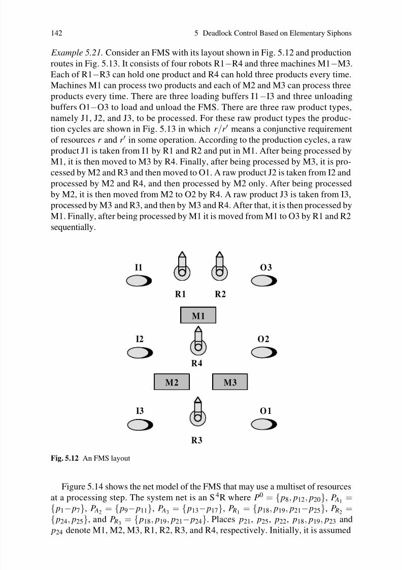
8/4/2019 Li Z., Zhou M. Deadlock Resolution in Automated Manufacturing Systems - A Novel Petri Net Approach
http://slidepdf.com/reader/full/li-z-zhou-m-deadlock-resolution-in-automated-manufacturing-systems-a-novel 156/249
142 5 Deadlock Control Based on Elementary Siphons
Example 5.21. Consider an FMS with its layout shown in Fig. 5.12 and production
routes in Fig. 5.13. It consists of four robots R1−R4 and three machines M1−M3.
Each of R1−R3 can hold one product and R4 can hold three products every time.
Machines M1 can process two products and each of M2 and M3 can process three
products every time. There are three loading buffers I1−I3 and three unloadingbuffers O1−O3 to load and unload the FMS. There are three raw product types,
namely J1, J2, and J3, to be processed. For these raw product types the produc-
tion cycles are shown in Fig. 5.13 in which r /r ′ means a conjunctive requirement
of resources r and r ′ in some operation. According to the production cycles, a raw
product J1 is taken from I1 by R1 and R2 and put in M1. After being processed by
M1, it is then moved to M3 by R4. Finally, after being processed by M3, it is pro-
cessed by M2 and R3 and then moved to O1. A raw product J2 is taken from I2 and
processed by M2 and R4, and then processed by M2 only. After being processed
by M2, it is then moved from M2 to O2 by R4. A raw product J3 is taken from I3,
processed by M3 and R3, and then by M3 and R4. After that, it is then processed by
M1. Finally, after being processed by M1 it is moved from M1 to O3 by R1 and R2
sequentially.
M 1
M 2
R 1
I 1 O 3
R 2
I 2
R 4
O 2
M 3
R 3
I 3 O 1
Fig. 5.12 An FMS layout
Figure 5.14 shows the net model of the FMS that may use a multiset of resources
at a processing step. The system net is an S4
R where P0
= p8, p12, p20, P A1 = p1− p7, P A2= p9− p11, P A3
= p13− p17, P R1= p18, p19, p21− p25, P R2
= p24, p25, and P R3
= p18, p19, p21− p24. Places p21, p25, p22, p18, p19, p23 and
p24 denote M1, M2, M3, R1, R2, R3, and R4, respectively. Initially, it is assumed
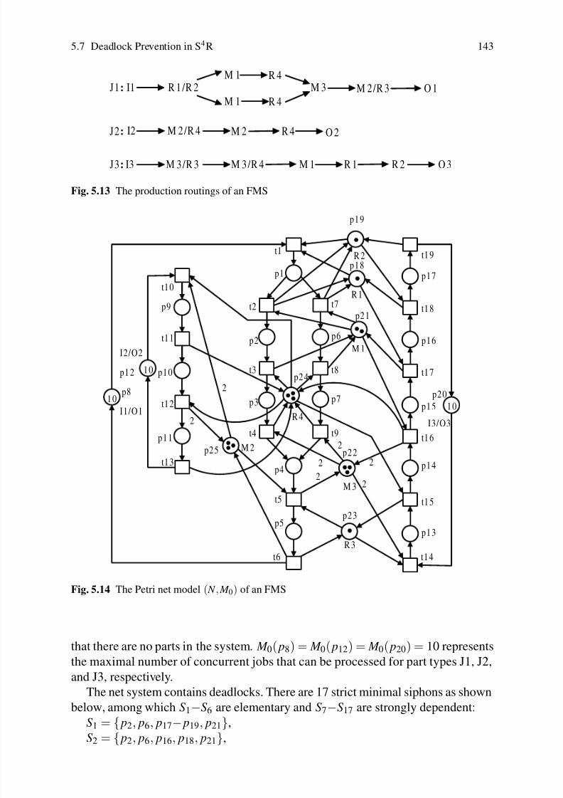
8/4/2019 Li Z., Zhou M. Deadlock Resolution in Automated Manufacturing Systems - A Novel Petri Net Approach
http://slidepdf.com/reader/full/li-z-zhou-m-deadlock-resolution-in-automated-manufacturing-systems-a-novel 157/249
5.7 Deadlock Prevention in S4R 143
I1M 1 R 4
M 1 R 4
J 1: R 1 / R 2 M 3 M 2 / R 3 O 1
J 2: I 2 M 2 / R 4 M 2 R 4 O 2
J 3: I 3 M 3 / R 3 M 3 / R 4 M 1 R 1 R 2 O 3
Fig. 5.13 The production routings of an FMS
t 1
t 2
t 3
t 4
t 5
t 6
t 7
t 8
t 9
t 1 0
t 1 1
t 1 2
t 1 3
t 1 4
t 1 5
t 1 6
t 1 7
t 1 8
t 1 9
p 1
p 2
p 3
p 4
p 5
p 6
p 7p 8
I 1 / O 1
p 9
p 1 0
p 1 1
p 1 2
I 2 / O 2
p 1 3
p 1 4
p 1 5
p 1 6
p 1 7
p 2 0
I 3 / O 3
p 1 8
R 1
p 1 9
R 2
p 2 1
M 1
p 2 2
M 3
2
2
2
2
2
p 2 3
R 3
p 2 4
R 4
2
2
p 2 5 M 2
1 0
1 01 0
Fig. 5.14 The Petri net model ( N , M 0) of an FMS
that there are no parts in the system. M 0( p8) = M 0( p12) = M 0( p20) = 10 represents
the maximal number of concurrent jobs that can be processed for part types J1, J2,
and J3, respectively.
The net system contains deadlocks. There are 17 strict minimal siphons as shown
below, among which S1−S6 are elementary and S7−S17 are strongly dependent:
S1 = p2, p6, p17− p19, p21,
S2 = p2, p6, p16, p18, p21,

8/4/2019 Li Z., Zhou M. Deadlock Resolution in Automated Manufacturing Systems - A Novel Petri Net Approach
http://slidepdf.com/reader/full/li-z-zhou-m-deadlock-resolution-in-automated-manufacturing-systems-a-novel 158/249
144 5 Deadlock Control Based on Elementary Siphons
S3 = p5, p9, p11, p14, p22, p24, p25,
S4 = p5, p9, p11, p14, p22− p24,
S5 = p4, p9, p11, p14, p22, p24,
S6 = p3, p7, p9, p11, p15, p21, p24,
S7 = p5, p9, p11, p17− p19, p21, p22, p24, p25,S8 = p5, p9, p11, p16, p18, p21, p22, p24, p25,
S9 = p5, p9, p11, p15, p21, p22, p24, p25,
S10 = p5, p9, p11, p17− p19, p21− p24,
S11 = p5, p9, p11, p16, p18, p21− p24,
S12 = p5, p9, p11, p15, p21− p24,
S13 = p4, p9, p11, p17− p19, p21, p22, p24,
S14 = p4, p9, p11, p16, p18, p21, p22, p24,
S15 = p4, p9, p11, p15, p21, p22, p24,
S16
=
p3, p
7, p
9, p
11, p
17− p
19, p
21, p
24,
S17 = p3, p7, p9, p11, p16, p18, p21, p24.
This system contains seven resources, leading to seven minimal P-semiflows:
I p18= p1 + p16 + p18,
I p19= p1 + p17 + p19,
I p21= p2 + p6 + p15 + p21,
I p22= 2 p4 + 2 p13 + 2 p14 + p22,
I p23= p5 + p13 + p23,
I p24= p3 + p7 + p9 + p11 + p14 + p24,
I p25= p5 + 2 p9 + 2 p10 + p25.
Note that M 0( p18) = 1, M 0( p19) = 1, M 0( p21) = 2, M 0( p22) = 3, M 0( p23) = 1,
M 0( p24) = 3, and M 0( p25) = 3. The number of tokens in each siphon under the
initial marking can be easily computed.
Six monitors V S1−V S6
are respectively added for S1 − S6. We take the control of
S3 = p5, p9, p11, p14, p22, p24, p25 as an example.
We have T h(S3) = p3 + 2 p4 + p7 + 2 p10 + 2 p13 and PS3= P1
S3∪P2
S3∪P3
S3,
where P1S3
= p1, p2, p3, p4, p6, p7, P2S3
= p9, p10, and P3S3
= p13. Accord-
ingly, we have k S3( p1) = k S3
( p2) = k S3( p3) = k S3
( p6) = k S3( p7) = k S3
( p4) = 2,
k S3
( p9) = k S3
( p10) = 2, and k S3
( p13) = 2.
∀ p
∈P R
∪P0
∪ p5, p11, p14, p15, p16, p17
,
k S3( p) = 0. As a result, gS3
= k S3+V S3
= 2 p1 +2 p2 +2 p3 +2 p4 +2 p6 +2 p7 +2 p9 +2 p10 + 2 p13 +V S3
.
By
∑r ∈S R3
I r = I p22+ I p24
+ I p25= (2 p4 + 2 p13 + 2 p14 + p22) + ( p9 + p11 + p3 + p7 +
p14 + p24) + (2 p9 + 2 p10 + p5 + p25),
we have
f S3=∑r ∈S R
3 I r −gS3
= p5 + p9 + p11 + 3 p14 + p22 + p24 + p25 −V S3−2 p1 −2 p2 −
p3 − 2 p6 − p7.
Clearly,||
f S3 ||− ∩
S3 =
/ 0 and||
f S3 ||
+
=S
3are true. Considering
M 0(S3) = M 0( p22) + M 0( p24) + M 0( p25) = 9
and
ω (S3) = ∑ p∈S f S3(max p• − 1) = (max p•
22− 1) + (max p•
25−1) = 2,

8/4/2019 Li Z., Zhou M. Deadlock Resolution in Automated Manufacturing Systems - A Novel Petri Net Approach
http://slidepdf.com/reader/full/li-z-zhou-m-deadlock-resolution-in-automated-manufacturing-systems-a-novel 159/249
5.7 Deadlock Prevention in S4R 145
we have 2 < ξS3< 9. In an analogous way, monitors V S1
, V S2, V S4
, V S5, and V S6
can
be accordingly added to the plant net model. The controlled system is denoted by
( N V , M 0V ) as shown in Fig. 5.15. The details concerning the control of elementary
siphons are given as follows:
(1) S1:∑r ∈S R
1 I r = 2 p1 + p2 + p6 + p15 + p16 + p17 + p18 + p19 + p21;
T h(S1) = 2 p1 + p15 + p16;
k S1= 2 p1 + p13 + p14 + p15 + p16;
gS1= 2 p1 + p13 + p14 + p15 + p16 +V S1
;
f S1= p2 + p6 + p17 + p18 + p19 + p21 −V S1
− p13 − p14;
M 0V (V S1) = 4 −ξS1
;
0 < ξS1≤ 3.
(2) S2:
∑r ∈S R2 I r = p1 + p2 + p6 + p15 + p16 + p18 + p21;T h(S2) = p1 + p15;
k S2= p1 + p13 + p14 + p15;
gS2= p1 + p13 + p14 + p15 +V S2
;
f S2= p2 + p6 + p16 + p18 + p21 −V S2
− p13 − p14;
M 0V (V S2) = 3 −ξS2
;
0 < ξS2≤ 2.
(3) S3:
∑r ∈S R3
I r = p3 +2 p4 + p5 + p7 +3 p9 +2 p10 + p11 +2 p13 +3 p14 + p22 + p24 + p25;
T h(S3) = p3 + 2 p4 + p7 + 2 p10 + 2 p13;k S3
= 2 p1 + 2 p2 + 2 p3 + 2 p4 + 2 p6 + 2 p7 + 2 p9 + 2 p10 + 2 p13;
gS3= 2 p1 + 2 p2 + 2 p3 + 2 p4 + 2 p6 + 2 p7 + 2 p9 + 2 p10 + 2 p13 +V S3
;
f S3= p5 + p9 + p11 + 3 p14 + p22 + p24 + p25 −V S3
−2 p1 −2 p2 − p3 −2 p6 − p7;
M 0V (V S3) = 9 −ξS3
;
2 < ξS3≤ 8.
(4) S4:
∑r ∈S R4
I r = p3 + 2 p4 + p5 + p7 + p9 + p11 + 3 p13 + 3 p14 + p22 + p23 + p24;
T h(S4) = p3 + 2 p4 + p7 + 3 p13;
k S4 = 2 p1 + 2 p2 + 2 p3 + 2 p4 + 2 p6 + 2 p7 + 3 p13;gS4
= 2 p1 + 2 p2 + 2 p3 + 2 p4 + 2 p6 + 2 p7 + 3 p13 +V S4;
f S4= p5 + p9 + p11 + 3 p14 + p22 + p23 + p24 −V S4
−2 p1 −2 p2 − p3 −2 p6 − p7;
M 0V (V S4) = 7 −ξS4
;
1 < ξS4≤ 6.
(5) S5:
∑r ∈S R5
I r = p3 + 2 p4 + p7 + p9 + p11 + 2 p13 + 3 p14 + p22 + p24;
T h(S5) = p3 + p7 + 2 p13;
k S5= p1 + p2 + p3 + p6 + p7 + 2 p13;
gS5 = p1 + p2 + p3 + p6 + p7 + 2 p13 +V S5 ; f S5
= 2 p4 + p9 + p11 + 3 p14 + p22 + p24 −V S5− p1 − p2 − p6;
M 0V (V S5) = 6 −ξS5
;
1 < ξS5≤ 5.

8/4/2019 Li Z., Zhou M. Deadlock Resolution in Automated Manufacturing Systems - A Novel Petri Net Approach
http://slidepdf.com/reader/full/li-z-zhou-m-deadlock-resolution-in-automated-manufacturing-systems-a-novel 160/249
146 5 Deadlock Control Based on Elementary Siphons
(6) S6:
∑r ∈S R6
I r = p2 + p3 + p6 + p7 + p9 + p11 + p14 + p15 + p21 + p24;
T h(S6) = p2 + p6 + p14;
k S6= p1 + p2 + p6 + p13 + p14;
gS6 = p1 + p2 + p6 + p13 + p14 +V S6 ; f S6
= p3 + p7 + p9 + p11 + p15 + p21 + p24 −V S6− p1 − p13;
M 0V (V S6) = 5 −ξS6
;
0 < ξS6≤ 4.
Table 5.6 shows the controllability of all dependent siphons by Theorem 5.10.
Algorithm 5.3 adds six monitors for the elementary siphons with ξS1= 1, ξS2
= 1,
ξS3= 3, ξS4
= 2, ξS5= 2, and ξS6
= 4, which can ensure the controllability of all
dependent siphons. Accordingly, we have M 0V (V S1) = 3, M 0V (V S2
) = 2, M 0V (V S3)
= 6, M 0V (V S4) = 5, M 0V (V S5
) = 4 and M 0V (V S6) = 1, as shown in Fig. 5.15.
Table 5.6 Controllability of dependent siphons
Siphon T -vector relationship Controllability
S7 ηS7= ηS1
+ηS3+ηS6
ξS1+ξS3
+ξS6> 7
S8 ηS8= ηS2
+ηS3+ηS6
ξS2+ξS3
+ξS6> 7
S9 ηS9= ηS3
+ηS6ξS3
+ξS6> 5
S10 ηS10= ηS1
+ηS4+ηS6
ξS1+ξS4
+ξS6> 6
S11 ηS11= ηS2
+ηS4+ηS6
ξS2+ξS4
+ξS6> 6
S12 ηS12= ηS4
+ηS6ξS4
+ξS6> 4
S13 ηS13
= ηS1
+ηS5
+ηS6
ξS1
+ξS5
+ξS6
> 6
S14 ηS14= ηS2
+ηS5+ηS6
ξS2+ξS5
+ξS6> 6
S15 ηS15= ηS5
+ηS6ξS5
+ξS6> 4
S16 ηS16= ηS1
+ηS6ξS1
+ξS6> 2
S17 ηS17= ηS2
+ηS6ξS2
+ξS6> 2
Alternatively, a set of control depth variables of the elementary siphons can be
found by solving the following LPP:
z = min6
∑i=1ξSi
s.t.
ξS1+ξS3
+ξS6> 7,
ξS2+ξS3
+ξS6> 7,
ξS3+ξS6
> 5,
ξS1+ξS4
+ξS6> 6,
ξS2+ξS4
+ξS6> 6,
ξS4+ξS6
> 4,
ξS1 +ξS5 +ξS6 > 6,ξS2
+ξS5+ξS6
> 6,
ξS5+ξS6
> 4,
ξS1+ξS6
> 2,

8/4/2019 Li Z., Zhou M. Deadlock Resolution in Automated Manufacturing Systems - A Novel Petri Net Approach
http://slidepdf.com/reader/full/li-z-zhou-m-deadlock-resolution-in-automated-manufacturing-systems-a-novel 161/249
5.7 Deadlock Prevention in S4R 147
t 1
t 2
t 3
t 4
t 5
t 6
t 7
t 8
t 9
t 1 0
t 1 1
t 1 2
t 1 3
t 1 4
t 1 5
t 1 6
t 1 7
t 1 8
t 1 9
p 1
p 2
p 3
p 4
p 5
p 6
p 7p 8
I 1 / O 1
p 9
p 1 0
p 1 1
p 1 2
I 2 / O 2
p 1 3
p 1 4
p 1 5
p 1 6
p 1 7
p 2 0
I 3 / O 3
p 1 8
R 1
p 1 9
R 2
p 2 1
M 1
p 2 2
M 3
2
2
2
2
2
p 2 3
R 3
p 2 4
R 4
2
2
p 2 5M 2
t 2
t 1 82
t 1 4
t 1 4
1 0
1 0
1 0
t 7
t 1 t 1 7
VS 2
t 2 t 1 4
t 1 t 1 5VS 5
t 9 t 1 4
t 4
2
2
4 t 1 t 1 6
VS 6
t 8 t 1 4
t 3
t 7
t 1
t 1 4
VS 122
3
t 5
t 1
t 1 5VS 42
23
3
5
t 1
t 1 0
t 1 2 t 5
t 1 52
22
2
2
2
VS 3
6
Fig. 5.15 The controlled system ( N V , M 0V )
ξS2+ξS6
> 2,
0 < ξS1≤ M 0(S1) − 1,
0 < ξS2≤ M 0(S2) − 1,
2 < ξS3≤ M 0(S3) − 1,
1 < ξS4≤ M 0(S4) − 1,
1 < ξS5≤ M 0(S5) − 1,
0 < ξS6≤ M 0(S6) − 1,
M 0(S1) −ξS1 ≥ maxV •S1 , M 0(S2) −ξS2
≥ maxV •S2,
M 0(S3) −ξS3≥ maxV •S3
,

8/4/2019 Li Z., Zhou M. Deadlock Resolution in Automated Manufacturing Systems - A Novel Petri Net Approach
http://slidepdf.com/reader/full/li-z-zhou-m-deadlock-resolution-in-automated-manufacturing-systems-a-novel 162/249
148 5 Deadlock Control Based on Elementary Siphons
M 0(S4) −ξS4≥ maxV •S4
,
M 0(S5) −ξS5≥ maxV •S5
,
M 0(S6) −ξS6≥ maxV •S6
,
maxV •S1
= 2,
maxV •S2= 1,
maxV •S3= 2,
maxV •S4= 3,
maxV •S5= 2,
maxV •S6= 1,
M 0(S1) = 4,
M 0(S2) = 3,
M 0(S3) = 9,
M 0(S4) = 7,
M 0(S5) = 6,
M 0(S6) = 5.
Solving the above LPP gives an optimal solution z∗ = 13 with ξS1= 1, ξS2
= 1,
ξS3= 3, ξS4
= 2, ξS5= 2, and ξS6
= 4. Also, it is easy to verify that ∀i ∈1,2, . . . ,6,
M min(Si) ≥ ξSi. This leads to M 0V (V S1
) = 3, M 0V (V S2) = 2, M 0V (V S3
) = 6, M 0V (V S4)
= 5, M 0V (V S5) = 4 and M 0V (V S6
) = 1. As a result, a live controlled system with six
monitors can be obtained by solving LPP.
Remark 5.2. It is found by Chao [8] that max-cs property is rather conservative.That is to say, a siphon that is not max-controlled does not necessarily lead to dead
transitions. A new concept called max’-controlled siphons is accordingly developed.
However, the way of adding a monitor such that a siphon is max’-controlled is not
presented. In this sense, making a siphon max’-controlled via the addition of a mon-
itor remains open. ⊓⊔
5.8 Bibliographical Remarks
Deadlock is a major issue that must be addressed in contemporary resource allo-
cation systems. Deadlocks and related blocking phenomena not only degrade the
productivity of a system but also lead to catastrophic results in some highly au-
tomated systems, e.g., semiconductor manufacturing systems [17]. Their efficient
handling becomes a necessary condition for a system to gain high throughput and
safety. This is the reason why this problem is extensively investigated in the litera-
ture, particularly within the area of flexible manufacturing systems [14, 21, 56, 57].
Deadlock is first addressed by computer scientists [10, 22, 23, 26, 48]. Some im-
portant results about deadlocks in Petri nets are obtained by Commoner in 1972 [13].
Handling deadlock prevention in manufacturing dates back to 1990 due to the sem-
inal work by Roszkowska and Viswanadham et al. [2, 43–46, 55]. The last two
decades have seen much effort for deadlock control in flexible manufacturing [15].

8/4/2019 Li Z., Zhou M. Deadlock Resolution in Automated Manufacturing Systems - A Novel Petri Net Approach
http://slidepdf.com/reader/full/li-z-zhou-m-deadlock-resolution-in-automated-manufacturing-systems-a-novel 163/249
5.8 Bibliographical Remarks 149
The work of Fanti and Zhou [17] surveys a variety of deadlock control ap-
proaches that are based on graph theory, automata, and Petri nets in the literature.
A survey and comparison of Petri net-based deadlock prevention policies for FMS
can be found in [36]. Also readers are referred to the books [28] and [42].
Problems and Discussions
5.1. For an S3PR, the existence of a liveness-enforcing supervisor with monitors
that are added for elementary siphons only depends on the presence of a feasible
solution to the following LPP:
min
m
∑i=1ξSi (5.8)
s.t.
M 0(S D j) >m
∑i=1
( M 0(Si) −ξSi), j = 1,2, . . . ,n,
1 ≤ ξSi≤ M 0(Si) −1, i = 1,2, . . . ,m,
where Π D = S D j| j = 1,2, . . . ,n and Π E = Si|i = 1,2, . . . ,m are the sets of de-
pendent and elementary siphons, respectively.
Can it be proved that LPP (5.8) definitely has a feasible solution for an S3PR
with acceptable initial markings?
5.2. Design a liveness-enforcing supervisor for the net shown in Fig. 5.8 by the
deadlock prevention policy presented in Sect. 5.6.
5.3. The net ( N , M 0) shown in Fig. 5.16 is the model of an FMS consisting of four
machine tools and two robots. Two types of parts can be produced in this system. It
is an S3PR where p1 and p8 are idle process places, p14− p19 are resource places,
and the others are operation places.
1. Find all the strict minimal siphons.
2. By the elementary siphon identification algorithm, compute the set of elementary
siphons. Check whether there exists a liveness-enforcing supervisor by explicitly
controlling its elementary siphons only.
3. According to the definition of the elementary siphons in a Petri net, they are not
unique. Suppose that a net has n siphons and rank ([η]) = m. We can at most findn!/(m!(n − m)!) different sets of elementary siphons. By using this example,
compare the permissive behavior of the supervisors resulting from controlling
different sets of elementary siphons.

8/4/2019 Li Z., Zhou M. Deadlock Resolution in Automated Manufacturing Systems - A Novel Petri Net Approach
http://slidepdf.com/reader/full/li-z-zhou-m-deadlock-resolution-in-automated-manufacturing-systems-a-novel 164/249
150 5 Deadlock Control Based on Elementary Siphons
t 1
t 2 t 3
t 4t 5
t 6
t 7
t 8t 9
t 1 0
t 1 1
t 1 2
t 1 3
t 1 4
p 1
p 2
p 3
p 4
p 5
p 6
p 7
p 8
p 9
p 1 0
p 1 1
p 1 2
p 1 3
p 1 4
M 1
p 1 5
M 2
p 1 6
M 3
p 1 7
M 4
p 1 8
R 1
p 1 9
R 2
6
6
Fig. 5.16 An S3PR net ( N , M 0)
5.4. The development of a deadlock prevention policy without the complete siphon
enumeration of a plant Petri net model can be first traced to the work by Huang et
al. [24] in which an algorithm that extracts a strict minimal siphon from an unmarked
maximal siphon is proposed. However, the algorithm is problematic. The corrections
are given in [34].
The deadlock prevention policy in [24] consists of two phases: siphon control
and control-induced siphon control. However, in each control phrase, the concept of
elementary siphons is not considered. Design a novel deadlock control policy based
on the policy in [24] by considering the existence of elementary siphons in each
phrase. Take the nets shown in Figs. 5.8 and 5.16 as examples.
5.5. One of the most important contributions in the development of deadlock control
strategies is due to Park and Reveliotis. In [40], a deadlock prevention policy is
proposed for S4R, which is of polynomial complexity. By this deadlock prevention
policy, design a liveness-enforcing supervisor for the net shown in Fig. 5.5.
5.6. Iterative siphon control for deadlock prevention is a good but old idea. A ba-
sic iterative siphon control approach [27, 39] for plant net model ( N , M 0) can be
generalized as follows:
i := 0
Π (0) = / 0
N (0) := N
M (0) := M 0

8/4/2019 Li Z., Zhou M. Deadlock Resolution in Automated Manufacturing Systems - A Novel Petri Net Approach
http://slidepdf.com/reader/full/li-z-zhou-m-deadlock-resolution-in-automated-manufacturing-systems-a-novel 165/249
5.8 Bibliographical Remarks 151
i := i + 1
Find the set Π (i) of minimal siphons of N (i−1) not belonging to ∪i−1k =0Π
(k )
repeat
Implement on ( N (i−1), M (i−1)) the set of GMECs [20] λ T S M ≥ 1,∀S ∈ Π (i)
and denote the resultant net by ( N (i)
, M (i)
)i := i + 1
Find the set Π (i) of minimal siphons of N (i−1) not belonging to ∪i−1k =0Π
(k )
until Π (i) = / 0
output ( N (i), M (i))
Using the iterative siphon control scheme mentioned above, design a liveness-
enforcing supervisor for the net shown in Fig. 5.8. It is worth noting that this algo-
rithm is effective if at each iteration step, the net that is handled is ordinary. In the
process of iterations, a generalized net may be produced. We refer the reader to the
work in [27,29], and [41] to complete the iteration for this example. Decide whetheran optimal liveness-enforcing supervisor can be found.
5.7. Implicit places [11, 12, 18, 19, 47] are a class of elements in a Petri net whose
removal does not change the behavior of the Petri net. For example, the deadlock
prevention policy proposed in [16] computes 18 monitors for the Petri net model
shown in Fig. 5.8. By considering the elementary siphons, however, the addition of
six monitors for the elementary siphons can lead to a live controlled system. Both
nets with the different number of monitors have the same behavior. Identify the
implicit places from the net that has 18 monitors and compare with the one that
has six monitors. The readers are suggested to pay attention to the computational
complexity of identifying implicit places and controllability decision of dependent
siphons [37].
5.8. The redundancy problem of the monitors that are added for siphon control is
also noticed by Iordache, Moody, and Antsaklis. Use the redundant monitor identifi-
cation method proposed in [27] to decide whether the monitors in the live controlled
system resulting from the deadlock prevention policy in [16] can be removed.
5.9. A redundant monitor identification method is proposed in [53] by using thecomplete state enumeration. Discuss its pros and cons.
5.10. Compare the computational burden by using INA [49] and the MIP-based
deadlock detection method [9] to find all the strict minimal siphons in differently
sized S3PR nets. Supposedly, the superiority of the MIP-based deadlock detection
method is more and more evident as a net size grows.
5.11. By Definitions 5.19 and 5.20, the deadlock prevention policy developed in [16]
guarantees that, at any reachable marking, the token count in the adjoint set of a
siphon does not exceed the initial number of tokens marked in the siphon. To beformal, the policy ensures that ∀S ∈Π , ∀ M ∈ R( N , M 0), M (PS) ≤ M 0(S) − 1. That
is to say, deadlocks in an S3PR can be prevented by enforcing the following set of
GMECs by monitors: ( L, B) = (li,bi)|li = ∑ p∈PSi p,bi = M 0(Si) −1.

8/4/2019 Li Z., Zhou M. Deadlock Resolution in Automated Manufacturing Systems - A Novel Petri Net Approach
http://slidepdf.com/reader/full/li-z-zhou-m-deadlock-resolution-in-automated-manufacturing-systems-a-novel 166/249
152 5 Deadlock Control Based on Elementary Siphons
By using the results presented in Chap. 4, a set of monitors that are added for
elementary constraints only may enforce all GMECs in the set.
The Petri net ( N , M 0) in Fig. 5.3 is an S3PR if P0 = p1, p10, P R = p11, p12, p13, p14, p15, and others are operation places. There are three strict minimal siphons
S1 = p5, p9, p12, p13, S2 = p4, p6, p13, p14, and S3 = p6, p9, p12, p13, p14.The adjoint sets of the three siphons are PS1= p3, p4, p7, p8, PS2
= p3, p5,
p7, p8, and PS3= p3, p4, p5, p7, p8.
1. List the set of GMECs for this Petri net to implement the deadlock prevention
policy in [16].
2. Find a monitor solution in which only elementary constraints are explicitly con-
trolled.
3. Compare the two supervisors found by this GMEC-based method and the policy
in [16].
4. Check whether there exist implicit places in the supervisor that is computed bythe GMEC-based method.
5. By the MIP-based deadlock detection method, check whether there exist redun-
dant monitors whose removal keeps the liveness of the resultant net systems.
p 5
p 1 4
p 1 3
p 1 5
p 8
p 7
p 6
p 1 1
p 1 2
t 1 2
p 1
p 1 0
p 9
p 4p 3
p 2
p 1 6
t 1 1
t 1 0
t 9
t 8
t 6
t 7
t 5
t 4
t 3
t 2
t 1
Fig. 5.17 An S3PR net ( N , M 0)
5.12. Redo (1)−(5) of Problem 5.11 for the Petri net model of the FMS in Example
5.12.

8/4/2019 Li Z., Zhou M. Deadlock Resolution in Automated Manufacturing Systems - A Novel Petri Net Approach
http://slidepdf.com/reader/full/li-z-zhou-m-deadlock-resolution-in-automated-manufacturing-systems-a-novel 167/249
5.8 Bibliographical Remarks 153
5.13. Let S1 = p5, p9, p10, p11, p12, p13, S2 = p3, p4, p9, p10, p11, p12, S3 = p2, p3, p9, p10, p11, and S4 = p5, p7, p12, p13. Construct an S3PR N such that
Π = S1,S2,S3,S4 is the set of strict minimal siphons of N . Verify whether the net
shown in Fig. 5.18 is such an S3PR.
5.14. Let S1 = p5, p9, p10, p11, p12, p13, p16, S2 = p5, p8, p11, p12, p13, p16, S3 = p2, p9, p10, p11, and S4 = p5, p7, p12, p13. Construct an S3PR N such that Π =S1,S2,S3,S4 is the set of strict minimal siphons of N . Verify whether the net shown
in Fig. 5.17 is such an S3PR.
5.15. Let S1 = p1, p2,r 1,r 2 and S2 = p3, p4,r 2,r 3,r 4. Find an S3PR N = (P0 ∪P A ∪ P R,T ,F ) such that Π E = S1,S2, where p1− p4 ⊆ P A and r 1−r 4 ⊆ P R.
5.16. Let Π E = Si|i ∈ Nn. Develop an algorithm that can construct an S3PR N =
(P0
∪ P A ∪ P R,T ,F ) such that Π E is a set of elementary siphons of N .
p 5
p 1 4
p 1 3
p 1 5
p 8
p 7
p 6
p 1 1
p 1 2
p 1
p 1 0
p 9
p 4p 3
p 2
t 1 2
t 1 1
t 1 0
t 9
t 8
t 6
t 7
t 5
t 4
t 3
t 2
t 1
Fig. 5.18 An S3PR net ( N , M 0)
5.17. Properly set parameters w1−w12, x, y, and z for the net in Fig. 5.19 such that
its liveness is independent from the non-zero initial markings d 1 and d 2 of places p4
and p5, respectively.
5.18. Prove Theorem 5.12. Hint: We refer the reader to the proof of Theorem VI.I
in [16].

8/4/2019 Li Z., Zhou M. Deadlock Resolution in Automated Manufacturing Systems - A Novel Petri Net Approach
http://slidepdf.com/reader/full/li-z-zhou-m-deadlock-resolution-in-automated-manufacturing-systems-a-novel 168/249
154 5 Deadlock Control Based on Elementary Siphons
p 4
p 5
p 7
p 6
p 1 0
p 1 1
t 5
t 6
t 7
p 1
p 9p 8
p 3
p 2
t 8
t 4
t 3
t 2
t 1
z
x
y
w 1 0
w 1 1w 9
w 8
w 7
w 6
w 5
w 3
w 4w 2
w 1
w 1 2
d1 d2
Fig. 5.19 An S4R net ( N , M 0)
References
1. Abdallah, I.B., ElMaraghy, H.A. (1998) Deadlock prevention and avoidance in FMS: A Petri
net based approach. International Journal of Advanced Manufacturing Technology, vol.14,
no.10, pp.704–715.
2. Banaszak, Z., Roszkowska, E. (1988) Deadlock avoidance in pipeline concurrent processes.
Podstawy Sterowania (Foundations of Control), vol.18, no.1, pp.3–17.
3. Barkaoui, K., Abdallah, I.B. (1996) Analysis of a resource allocation problem in FMS using
structure theory of Petri nets. In Proc. 1st Int. Workshop on Manufacturing and Petri Nets,
pp.62–76.
4. Barkaoui, K., Pradat-Peyre, J.F. (1996) On liveness and controlled siphons in Petri nets. In
Proc. 17th Int. Conf. on Applications and Theory of Petri Nets Lecture Notes in Computer
Science, vol.1091, pp.57–72.
5. Barkaoui, K., Chaoui, A., Zouari, B. (1997) Supervisory control of discrete event systems
based on structure theory of Petri nets. In Proc. IEEE Int. Conf. on Systems, Man, and Cyber-
netics, pp.3750–3755.
6. Chao, D.Y. (2006) An incremental approach to extracting minimal bad siphons, International
Journal of Information Science and Engineering, vol.23, no.1, pp.203–214.
7. Chao, D.Y. (2006) Computation of elementary siphons for deadlock control. The Computer
Journal, vol.49, no.4, pp.470–479.
8. Chao, D.Y. (2007) Max′-controlled siphons for liveness of S3PGR2. IET Control Theory and
Applications, vol.1, no.4, pp.933–936.
9. Chu, F., Xie, X.L. (1997) Deadlock analysis of Petri nets using siphons and mathematical
programming. IEEE Transactions on Robotics and Automation, vol.13, no.6, pp.793–804.
10. Coffman, E.G., Elphick, M.J., Shoshani, A. (1971) Systems deadlocks. ACM Computing Sur-
veys, vol.3, no.2, pp.67–78.
11. Colom, J.M., Silva, M. (1989) Improving the linearly based characterization of P/T nets. In
Proc. 10th Int. Conf. on Applications and Theory of Petri Nets, G. Rozenberg (Ed.), Lecture Notes in Computer Science, vol.483, pp.113–145.
12. Colom, J.M., Campos, J., Silva, M. (1990) On liveness analysis through linear algebraic tech-
niques. In Proc. of Annual General Meeting of ESPRIT Basic Research Action 3148 Design
Methods Based on Nets DEMON .

8/4/2019 Li Z., Zhou M. Deadlock Resolution in Automated Manufacturing Systems - A Novel Petri Net Approach
http://slidepdf.com/reader/full/li-z-zhou-m-deadlock-resolution-in-automated-manufacturing-systems-a-novel 169/249
References 155
13. Commoner, F. (1972) Deadlocks in Petri nets. Report CA-7206-2311, Massachusetts Com-
puter Associates, Wakefield, Massachusetts.
14. D’souza, K.A., Khator, S.K. (1994) A survey of Petri nets in automated manufacturing sys-
tems control. Computers in Industry Engineering, vol.24, no.1, pp.5–16.
15. D’souza, K.A., Khator, S.K. (1997) System reconfiguration to avoid deadlocks in automated
manufacturing systems. Computers in Industry Engineering, vol.32, no.2, pp.455–465.16. Ezpeleta, J., Colom, J.M., Martinez, J. (1995) A Petri net based deadlock prevention policy
for flexible manufacturing systems. IEEE Transactions on Robotics and Automation, vol.11,
no.2, pp.173–184.
17. Fanti, M.P., Zhou, M.C. (2004) Deadlock control methods in automated manufacturing sys-
tems. IEEE Transactions on Systems, Man, and Cybernetics, Part A, vol.34, no.1, pp.5–22.
18. Garcıa-Valles, F., Colom, J.M. (1999) Implicit places in net systems. In Proc. 8th Int. Work-
shop on Petri Nets and Performance Models, pp.104–113.
19. Garcıa-Valles, F., Colom, J.M. (2002) Checking redundancy in supervisory control. A com-
plexity result. In Proc. 15th IFAC World Congress on Automatic Control.
20. Giua, A., DiCesare, F., Silva, M. (1992) Generalized mutual exclusion constraints on nets
with uncontrollable transitions. In Proc. IEEE Int. Conf. on Systems, Man, and Cybernetics,pp.974–979.
21. Giua, A., Seatzu, C. (2007) A systems theory view of Petri nets. In Advances in Control
Theory and Applications, Lecture Notes in Control and Information Science, vol.353, C.
Bonivento et al. (Eds.), pp.99–127.
22. Gold, E.M. (1978) Deadlock predication: Easy and difficult cases. SIAM Journal of Comput-
ing, vol.7, no.3, pp.320–336.
23. Haberman, A. (1969) Prevention of system deadlocks. Communications of the ACM , vol.12,
no.7, pp.373–377.
24. Huang, Y.S., Jeng, M.D., Xie, X.L., Chung, S. L. (2001) Deadlock prevention policy based on
Petri nets and siphons. International Journal of Production Research, vol.39, no.2, pp.283–
305.
25. Huang, Y.S., Jeng, M.D., Xie, X.L., Chung, S.L. (2001) A deadlock prevention policy for
flexible manufacturing systems using siphons. In Proc. IEEE Int. Conf. on Robotics and Au-
tomation, pp.541–546.
26. Isloor, S.S., Marsland, T.A. (1980) The deadlock problem: An overview. Computer , vol.13,
no.9, pp.58–77.
27. Iordache, M.V., Moody, J.O., Antsaklis, P.J. (2002) Synthesis of deadlock prevention supervi-
sors using Petri nets. IEEE Transactions on Robotics and Automation, vol.18, no.1, pp.59–68.
28. Iordache, M.V., Antsaklis, P.J. (2006) Supervisory Control of Concurrent Systems: A Petri
Net Structural Approach. Berlin: Springer.
29. Lautenbach, K., Ridder, H. (1996) The linear algebra of deadlock avoidance−a Petri net
approach. No.25-1996, Technical Report, Institute of Software Technology, University of
Koblenz-Landau, Koblenz, Germany.30. Li, Z.W., Zhou, M.C. (2004) Elementary siphons of Petri nets and their application to dead-
lock prevention in flexible manufacturing systems. IEEE Transactions on Systems, Man, and
Cybernetics, Part A, vol.34, no.1, pp.38–51.
31. Li, Z.W., Uzam, M., Zhou, M.C. (2004) Comments on “Deadlock prevention policy based
on Petri nets and siphons”. International Journal of Production Research, vol.42, no.24,
pp.5253–5254.
32. Li, Z.W., Zhou, M.C. (2006) Two-stage method for synthesizing liveness-enforcing super-
visors for flexible manufacturing systems using Petri nets. IEEE Transactions on Industrial
Informatics, vol.2, no.4, pp.313–325.
33. Li, Z.W., Hu, H.S., Wang, A.R. (2007) Design of liveness-enforcing supervisors for flexible
manufacturing systems using Petri nets. IEEE Transactions on Systems, Man, and Cybernet-ics, Part C , vol.37, no.4, pp.517–526.
34. Li, Z.W., Liu, D. (2007) A correct minimal siphons extraction algorithm from a maximal
unmarked siphon of a Petri net. International Journal of Production Research, vol.45, no.9,
pp.2163–2167.

8/4/2019 Li Z., Zhou M. Deadlock Resolution in Automated Manufacturing Systems - A Novel Petri Net Approach
http://slidepdf.com/reader/full/li-z-zhou-m-deadlock-resolution-in-automated-manufacturing-systems-a-novel 170/249
156 5 Deadlock Control Based on Elementary Siphons
35. Li, Z.W., Zhao, M. (2008) On controllability of dependent siphons for deadlock prevention in
generalized Petri nets. IEEE Transactions on Systems, Man, and Cybernetics, Part A, vol.38,
no.2, pp.369–384.
36. Li, Z.W., Zhou, M.C. (2008) A survey and comparison of Petri net-based deadlock preven-
tion policies for flexible manufacturing systems. IEEE Transactions on Systems, Man, and
Cybernetics, Part C , vol.38, no.2, pp.172–188.37. Li, Z.W. (2009) On systematic methods to remove redundant monitors from liveness-
enforcing net supervisors. To appear in Computer and Industrial Engineering.
38. Lindo, Premier Optimization Modeling Tools, http://www.lindo.com/.
39. Moody, J.O., Antsaklis, P.J. (1998) Supervisory Control of Discrete Event Systems Using Petri
Nets. Boston, MA: Kluwer.
40. Park, J., Reveliotis, S.A. (2001) Deadlock avoidance in sequential resource allocation systems
with multiple resource acquisitions and flexible routings. IEEE Transactions on Automatic
Control, vol.46, no.10, pp.1572–1583.
41. Piroddi, L., Cordone, R., Fumagalli, I. (2008) Selective siphon control for deadlock preven-
tion in Petri nets. IEEE Transactions on Systems, Man, and Cybernetics, Part A. vol. 38, no.
6, pp.1337–1348.42. Reveliotis, S.A. (2005) Real-time Management of Resource Allocation Systems: A Discrete
Event Systems Approach. New York: Springer.
43. Roszkowska, E. (1990) Deadlock avoidance in concurrent compound pipeline processes,
Archives of Theoretical and Engineering Informatics, vol.2, no.3–4, pp. 227–242.
44. Roszkowska, E. (1991) Application of Petri nets to the modelling and efficiency evaluation
of FMS, Ph.D. thesis (in Polish), Report 4/91, Institute of Engineering Cybernetics, Wroclaw
University of Technology, Poland.
45. Roszkowska, E., Wojcik, R. (1993) Problems of process flow feasibility in FAS. In CIM in
Process and Manufacturing Industries, Oxford: Pergamon Press, pp.115–120.
46. Roszkowska, E., Jentink, J. (1993) Minimal restrictive deadlock avoidance in FMSs. In Proc.
European Control Conf., J. W. Nieuwenhuis, C. Pragman, and H. L. Trentelman, Eds., vol.2,
pp. 530–534.
47. Silva, M., Teruel, E., Colom, J.M. (1998) Linear algebraic and linear programming techniques
for the analysis of place/transition net systems. In Lectures on Petri Nets I: Basic Models,
Lectures Notes in Computer Science, vol.1491, W. Reisig and G. Rozenberg (Eds.), pp.309–
373.
48. Singhal, M. (1989) Deadlock detection in distributed systems. IEEE Computer , vol.22, no.11,
pp.37–48.
49. Starke, P.H. (2003) INA: Integrated Net Analyzer . http://www2.informatik.hu-berlin.de/ ∼starke/ina.html.
50. Tricas, F., Garcıa-Valles, F., Colom, J.M., Ezpeleta, J. (1998) A structural approach to the
problem of deadlock prevention in processes with shared resources. In Proc. 4th Workshop
on Discrete Event Systems, pp.273–278.
51. Tricas, F., Garcıa-Valles, F., Colom, J.M., Ezpeleta, J. (2000) An iterative method for dead-
lock prevention in FMSs. In Proc. 5th Workshop on Discrete Event Systems, R. Boel and
G.Stremersch (Eds.), pp.139–148.
52. Uzam, M., Zhou, M.C. (2006) An improved iterative synthesis method for liveness enforcing
supervisors of flexible manufacturing systems. International Journal of Production Research,
vol.44, no.10, pp.1987–2030.
53. Uzam, M., Li, Z.W., Zhou, M.C. (2007) Identification and elimination of redundant control
places in Petri net based liveness enforcing supervisors of FMS. International Journal of
Advanced Manufacturing Technology, vol.35, no.1–2, pp.150–168.
54. Uzam, M., Zhou, M.C. (2007) An iterative synthesis approach to Petri net based deadlock
prevention policy for flexible manufacturing systems. IEEE Transactions on Systems, Man,and Cybernetics, Part A, vol.37, no.3, pp.362–371.
55. Viswanadham, N., Narahari, Y., Johnson, T. (1990) Deadlock prevention and deadlock
avoidance in flexible manufacturing systems using Petri net models. IEEE Transactions on
Robotics and Automation, vol.6, no.6, pp.713–723.

8/4/2019 Li Z., Zhou M. Deadlock Resolution in Automated Manufacturing Systems - A Novel Petri Net Approach
http://slidepdf.com/reader/full/li-z-zhou-m-deadlock-resolution-in-automated-manufacturing-systems-a-novel 171/249
References 157
56. Wu, N.Q. (1999) Necessary and sufficient conditions for deadlock-free operation in flexible
manufacturing systems using a colored Petri net model. IEEE Transactions on Systems, Man,
and Cybernetics, Part C , vol.29, no.2, pp.192–204.
57. Wu, N.Q., Zhou, M.C. (2001) Avoiding deadlock and reducing starvation and blocking in
automated manufacturing systems. IEEE Transactions on Robotics and Automation, vol.17,
no.5, pp.658–669.58. Zouari, B., Barkaoui, K. (2003) Parameterized supervisor synthesis for a modular class of
discrete event systems. In Proc. IEEE Int. Conf. on Systems, Man, and Cybernetics, pp.1874–
1879.

8/4/2019 Li Z., Zhou M. Deadlock Resolution in Automated Manufacturing Systems - A Novel Petri Net Approach
http://slidepdf.com/reader/full/li-z-zhou-m-deadlock-resolution-in-automated-manufacturing-systems-a-novel 172/249
Chapter 6
Optimal Liveness-Enforcing Supervisors
Abstract This chapter considers the design of optimal, i.e., maximally permissive,
liveness-enforcing (Petri net) supervisors for automated manufacturing systems. It
first reviews a deadlock prevention policy that is based on theory of regions, which is
optimal. Then, based on the elementary siphon theory, sufficient conditions are pre-
sented under which there exists an optimal liveness-enforcing supervisor for a class
of Petri nets, S3PR (system of simple sequential processes with resources). A syn-
thesis method of such a supervisor is given if it exists. This chapter also shows that
an optimal liveness-enforcing supervisor can be computed in polynomial time if all
the siphons in an S3PR are elementary. Moreover, there exists an optimal liveness-
enforcing supervisor if the capacity of every resource is greater than one.
6.1 Background
The quality of a deadlock prevention policy can be shown by evaluating its resultant
controlled net system from a number of aspects. Usually, in addition to its structural
complexity, behavior permissiveness is one of the most important criteria in evalu-
ating the performance of a liveness-enforcing (Petri net) supervisor. In supervisorycontrol theory [22], the existence and synthesis approach of an optimal, i.e., max-
imally permissive, supervisor for a discrete-event system is well addressed in the
framework of formal languages and finite-state automata. When the control speci-
fication languages are controllable, the resultant automaton serves as a maximally
permissive supervisor by properly trimming the automaton that represents the be-
havior of a plant. Its computational complexity depends on the complete state enu-
meration. Results on the existence and synthesis of a liveness-enforcing marking-
based supervisor are reported by Sreenivas in [24–26]. It is shown that the existence
of a liveness-enforcing marking-based supervisor is undecidable for an arbitraryPetri net. In case of bounded Petri nets, it is decidable. However, the decision pro-
cedure requires the KM-tree of a Petri net, which is basically the reachability graph
of the net.
159

8/4/2019 Li Z., Zhou M. Deadlock Resolution in Automated Manufacturing Systems - A Novel Petri Net Approach
http://slidepdf.com/reader/full/li-z-zhou-m-deadlock-resolution-in-automated-manufacturing-systems-a-novel 173/249
160 6 Optimal Liveness-Enforcing Supervisors
The theory of regions [2, 9] can be used to synthesize pure Petri nets from
automaton-based models and is an important method for supervisory control of
discrete-event systems. By using the theory of regions, Uzam [28] develops an
optimal liveness-enforcing supervisor synthesis method for FMS. Later, in terms
of plain and popular linear algebra notions, Ghaffari et al. [11] explore the suffi-cient and necessary conditions on the existence of a liveness-enforcing supervisor
that is optimal, and develop a methodology to synthesize such a supervisor. The
most attractive advantage of these approaches is that such an optimal supervisor can
be always obtained if it exists. This chapter explores the existence of an optimal
liveness-enforcing supervisor, M ∗ for short, for S3PR nets in terms of elementary
siphons through pure structural analysis.
6.2 Optimal Supervisor Design by the Theory of Regions
Deadlock prevention or liveness enforcement is a special class of forbidden state
problems that are typical in supervisory control of discrete-event systems. In a Petri
net formalism, M F is usually used to denote the set of markings for which control
specifications do not hold in a Petri net ( N , M 0). Set M F is also called the set of
forbidden markings. The markings in it are hence unsafe [14]. To find a Petri net
supervisor for the given control specifications, the objective is to determine a set of
monitors that, once added to a given plant net model, prevent the whole system from
reaching these states. For example, the GMECs in Chap. 4 are also a typical class
of forbidden state problems.
Definition 6.1. The set M L of legal or admissible markings is the maximal set of
reachable markings such that (1) M L ∩M F = / 0, and (2) it is possible to reach initial
marking M 0 from any legal marking without leaving M L.
By Definition 6.1 we haveM L = R( N , M 0)\M F . Let Rc be the reachability graph
containing all legal markings for the given control specification in a plant Petri net
model ( N , M 0). It is clear that every element inM
L can be found in Rc and everynode in Rc is an element in M L. At any marking in M L, the system cannot be led
outsideM L. A marking inM L is called dangerous if an unsafe marking (in M F ) can
be possibly reached due to improper firing of an enabled transition. To solve the con-
trol problem, one has to identify the set of state/event separation instances (or mark-
ing/transition separation instances in net terminology) from an admissible marking
to a non-admissible one. The additional monitors are used to prevent these transi-
tions from occurring in order to keep the state space of the controlled system in the
set of legal markings. Formally, the set of marking/transition separation instances
that the supervisor has to disable isΩ =
( M ,t )| M [t
M ′
∧ M
∈M L
∧ M ′ /
∈M L
, where
M is a dangerous marking and M ′ is bad. LetM D be the set of dangerous markings.
Clearly, we have M D = M | M ∈M L ∧∃t ∈ T , ∋ M [t M ′∧ M ′∈M F .
An optimal supervisor is the one that ensures the reachability of all markings in
M L and forbids all marking/transition separation instances in Ω . An algorithm is

8/4/2019 Li Z., Zhou M. Deadlock Resolution in Automated Manufacturing Systems - A Novel Petri Net Approach
http://slidepdf.com/reader/full/li-z-zhou-m-deadlock-resolution-in-automated-manufacturing-systems-a-novel 174/249
6.2 Optimal Supervisor Design by the Theory of Regions 161
proposed in [11], which is of polynomial complexity with respect to the number of
states in the reachability graph of a plant net model. It can give legal behavior Rc,
M L, Ω , M D, and the set of transitions leading outside Rc.
Next we illustrate the above concepts. Let us consider an FMS with two machine
tools M1 and M2, each of which can process only one part at a time, and one robotR that can hold one part at a time. Parts enter the FMS through input/output buffers
I1/O1 and I2/O2. The system can repeatedly produce two part-types J1 and J2. The
production sequences are J1: M1→R→M2 and J2: M2→R→M1.
p 2
p 4
p 8
p 6
p 7p 3
p 9
p 5p 1
p 1 1
p 1 0
t 1 t 8
t 7
t 6
t 5t 4
t 3
t 2
I 2 / O 2I 1 / O 1
Fig. 6.1 The Petri net model ( N , M 0) of an FMS
Figure 6.1 shows the Petri net model, denoted by ( N , M 0), of the system, where
tokens in p1 and p5 indicate the maximal number of parts of J1 and J2, which can
be concurrently processed in the system, p2, p3, p4, p6, p7, and p8 represent the op-
erations on J1 and J2, and p9− p11 denote the availability of M1, R, and M2, respec-
tively. Its reachability graph is shown in Fig. 6.2 given M 0 = 3 p1 + 3 p5 + p9 + p10 + p11.
In the reachability graph of a Petri net, markings are generally categorized into
four classes in the sense of deadlock control: deadlock, bad, dangerous, and good
markings. A deadlock one means a dead system state by which no successive mark-
ing is followed. A bad one is the one that has subsequent markings, from which the
initial marking cannot be reached. A dangerous one can reach a good, bad or dead-
lock one depending on supervisory control. It is a node of the maximal strongly
connected component containing the initial marking and its son nodes are either
bad or deadlock ones. Good markings are the ones except deadlock, bad, and dan-gerous ones. Good and dangerous markings are included in the maximal strongly
connected component containing the initial marking and bad and deadlock ones are
not included in the component.

8/4/2019 Li Z., Zhou M. Deadlock Resolution in Automated Manufacturing Systems - A Novel Petri Net Approach
http://slidepdf.com/reader/full/li-z-zhou-m-deadlock-resolution-in-automated-manufacturing-systems-a-novel 175/249
162 6 Optimal Liveness-Enforcing Supervisors
In Fig. 6.2, M 13 and M 14 are deadlock and M 4, M 8, and M 9 are bad, while M 1, M 2,
M 3, M 5, M 6, and M 11 are dangerous. All the other markings are hence good. The set
of good and dangerous markings in R( N 0, M 0), denoted by M L, should constitute
the maximum legal behavior if a supervisory controller is optimally designed.
M 0
M 1 M 2M 3 M 5M 4
M 6 M 7
M 8 M 9
M 1 0 M 1 1
M 1 2M 1 3 M 1 4
M 1 5
M 1 6 M 1 7
M 1 8 M 1 9
t 1
t 2
t 4 t 5
t 6
t 7
t 8
t 4
t 4
t 4
t 1
t 1
t 3
t 3
t 5
t 5
t 5
t 5
t 5
t 1
t 7
t 2
t 1
t 8
t 8
t 8t 6
t 5
t 1
t 1t 2 t 6
t 1 t 5
g o o d m a r k i n g
d a n g e r o u s m a r k i n g
b a d m a r k i n g
d e a d l o c k m a r k i n g
Fig. 6.2 The reachability graph of the Petri net ( N , M 0)
As stated previously, a marking/transition separation instance has the form of
( M ,t ), where M is a dangerous marking, and t is a transition whose firing results
in marking M [t , which is a bad or deadlock marking. In Fig. 6.2, we have Ω =
( M
1,t
5),
( M
2,t
1),
( M
3,t
5),
( M
5,t
1),
( M
6,t
5),
( M
11,t
1).
The theory of regions is proposed for the synthesis of pure nets from given finite
transition systems [2], which can be adopted to synthesize the liveness-enforcing
supervisor for a plant net model [11].
Given a plant model ( N , M 0) of a system with n transitions to control and its Rc,
the theory of regions designs a monitor pm and then adds it to the original Petri net
for each marking/transition separation instance ( M ,t ) such that t is disabled at M .
Let ( N α , M α 0 ) be the resultant net with monitors. We need to compute M α 0 ( pm) and
[ N α ]( pm,T ).
Note that it shall be ensured that the addition of pm does not exclude the markings
in Rc, which implies that pm has to satisfy the following reachability condition (6.1)
and circuit equation (6.2):
M ( pm) = M α 0 ( pm) + [ N α ]( pm, ·)−→Γ M ≥ 0,∀ M ∈M L (6.1)

8/4/2019 Li Z., Zhou M. Deadlock Resolution in Automated Manufacturing Systems - A Novel Petri Net Approach
http://slidepdf.com/reader/full/li-z-zhou-m-deadlock-resolution-in-automated-manufacturing-systems-a-novel 176/249
6.2 Optimal Supervisor Design by the Theory of Regions 163
where Γ M is any non-oriented path in Rc from M 0 to M , and−→Γ M is the counting vec-
tor of the path Γ M , which denotes the algebraic sum of all occurrences of transitions
in Γ M .
Consider any non-oriented circuit γ in Rc. Applying the state equation to the
nodes in γ and summing them up give the following circuit equation:
∑t ∈T
[ N α ]( pm, t ) ·−→γ [t ] = 0,∀γ ∈ C (6.2)
where −→γ [t ] denotes the algebraic sum of all occurrences of t in γ and C is the set of
non-oriented circuits in Rc. −→γ is called the counting vector of γ . Note that different
circuits in Rc may have the same circuit equation when their counting vectors are
identical.
Furthermore, the addition of pm necessarily forbids the firing of t for mark-
ing/transition separation instance ( M ,t ). That is to say, M ( pm) + [ N
α
]( pm,t ) ≤ −1.Thanks to M ( pm) = M α 0 ( pm)+[ N α ]( pm, ·)−→Γ M , for every separation instance ( M ,t ),
we have the marking/transition separation equation
M α 0 ( pm) + [ N α ]( pm, ·)−→Γ M + [ N α ]( pm,t ) ≤ −1. (6.3)
We now use Figs. 6.1 and 6.2 to illustrate the above procedure.
Example 6.1. In Fig. 6.2, we have Ω = ( M 1,t 5), ( M 2,t 1), ( M 3,t 5), ( M 5,t 1), ( M 6,t 5),
( M 11,t 1). First consider ( M 1, t 5). We need to find a monitor pm1 to achieve this
marking/transition separation. Note that M α
0 ( pm1) ≥ 0 is trivial and for simplic-ity, let x = M α 0 ( pm1) and xi = [ N α ]( pm1, t i), where i ∈ 1,2, . . . ,8. M L has a to-
tal of 15 markings, i.e., M L = M 0− M 3, M 5− M 7, M 10− M 12, M 15− M 19. Also,
different circuits in Fig. 6.2 may have the same circuit equations. For example,
M 0t 1 M 1t 2 M 3t 3 M 7t 4 M 0 and M 12t 2 M 16t 1 M 18t 4 M 6t 3 M 12 are two circuits. It is easy to
verify that they have the same circuit equations.
For ( M 1,t 5), we have the following reachability condition equations (6.4)−(6.18),
two circuit equations (6.19) and (6.20), and marking/transition separation equation
(6.21).
x ≥ 0, (6.4)
x + x1 ≥ 0, (6.5)
x + x1 + x2 ≥ 0, (6.6)
x + x1 + x2 + x1 ≥ 0, (6.7)
x + x1 + x2 + x3 ≥ 0, (6.8)
x + x1 + x2 + x3 + x1 ≥ 0, (6.9)
x + x1 + x2 + x3 + x1 + x2 ≥ 0, (6.10) x + x1 + x2 + x3 + x1 + x2 + x1 ≥ 0, (6.11)
x + x5 ≥ 0, (6.12)
x + x5 + x6 ≥ 0, (6.13)

8/4/2019 Li Z., Zhou M. Deadlock Resolution in Automated Manufacturing Systems - A Novel Petri Net Approach
http://slidepdf.com/reader/full/li-z-zhou-m-deadlock-resolution-in-automated-manufacturing-systems-a-novel 177/249
164 6 Optimal Liveness-Enforcing Supervisors
x + x5 + x6 + x5 ≥ 0, (6.14)
x + x5 + x6 + x7 ≥ 0, (6.15)
x + x5 + x6 + x7 + x5 ≥ 0, (6.16)
x + x5 + x6 + x7 + x5 + x6
≥0, (6.17)
x + x5 + x6 + x7 + x5 + x6 + x5 ≥ 0, (6.18)
x1 + x2 + x3 + x4 = 0, (6.19)
x5 + x6 + x7 + x8 = 0, (6.20)
x + x1 + x5 ≤ −1. (6.21)
Solving inequalities (6.4)−(6.21), we get x = 1, x1 = −1, x2 = 1, x5 = −1, x6 = 1,
and x3 = x4 = x7 = x8 = 0. Hence monitor pm1 is accordingly added, as shown in
Fig. 6.3, to the original Petri net.
p 2
p 4
p 8
p 6
p 7p 3
p 9
p 5p 1
p 1 1
p 1 0
t 1
t 7
t 6
t 5t 4
t 3
t 2
I 2 / O 2I 1 / O 1
pm 1
pm 3
pm 2
t 8
Fig. 6.3 A controlled system ( N α , M α 0 )
Now we deal with marking/transition separation instance ( M 2, t 1). It is obvious
to see that the reachability and circuit equations for all marking/transition separation
instances are the same, i.e., (6.4)−(6.20), in this example. When we deal with a new
marking/transition separation instance, what we shall do is just to replace (6.21)
with the corresponding separation equation. The separation equation for ( M 2,t 1)
happens to be (6.21) as well. Hence we can say that pm1 has implemented ( M 2,t 1)as well. Similarly, we can find monitor pm2 that implements ( M 3,t 5) and ( M 6,t 5)and monitor pm3 that implements ( M 5,t 1) and ( M 11, t 1). Consequently, the resultant
controlled system with three monitors is live, as shown in Fig. 6.3.

8/4/2019 Li Z., Zhou M. Deadlock Resolution in Automated Manufacturing Systems - A Novel Petri Net Approach
http://slidepdf.com/reader/full/li-z-zhou-m-deadlock-resolution-in-automated-manufacturing-systems-a-novel 178/249
6.2 Optimal Supervisor Design by the Theory of Regions 165
Note that although the number of monitors to add is theoretically at most equal
to, practically much smaller than, the number of marking/transition separation in-
stances in the reachability graph of a Petri net, the number of the sets of inequalities
that we have to solve is actually equal to that of marking/transition separation in-
stances. This is so since we do not know whether a monitor can implement twoor more marking/transition separation instances until all the sets of inequalities are
already solved.
For example, there are 20 reachable markings in Fig. 6.2, where two of them
are deadlock markings and six are dangerous markings. Hence there are six mark-
ing/transition separation instances. We know that three monitors actually implement
all these six marking/transition separation instances only after we have solved all the
six sets of inequalities. This is one of the major disadvantages of the method.
The next result from [11] indicates the existence of an optimal liveness-enforcing
supervisor. A controlled system is said to be optimal if it results from the syn-
chronous synthesis of a plant net model and an optimal supervisor. For example,
the controlled net system shown in Fig. 6.3 is optimal since the supervisor with
three monitors is optimal.
Theorem 6.1. There exists an optimal liveness-enforcing supervisor for a plant
Petri net model ( N , M 0) iff there exist a set of monitors that implement all mark-
ing/transition separation instances of ( N , M 0).
Corollary 6.1. R( N α , M α 0 ) = M | M is a marking in Rc = M L if ( N α , M α 0 ) is an
optimal controlled system for ( N , M 0).
Remark 6.1. The synthesis methods of optimal liveness-enforcing supervisors in
[11] and [28] need the complete state enumeration of a plant net model, whose
computation is expensive or impossible when we deal with either a large-sized net
model, or a small-sized one with a large initial marking. The work of Ghaffari et
al. [11] shows that, in general, the existence of an optimal liveness-enforcing su-
pervisor M ∗ can be determined by first generating the reachability graph, and then
solving an LPP for each marking/transition separation instance. Unfortunately, the
number of LPPs that need to be solved is in theory exponential with respect to the
size of the plant net and the initial marking. Worst of all, the number of constraints
in such an LPP is in theory exponential with respect to the net size and the initial
marking. Although an LPP can be solved in polynomial time, the complexity of
the supervisor synthesis approach based on the theory of regions makes it actually
impractical.
The next section presents the existence conditions and synthesis method of an op-
timal liveness-enforcing supervisor for a class of Petri nets, S3PR, by pure structural
analysis.

8/4/2019 Li Z., Zhou M. Deadlock Resolution in Automated Manufacturing Systems - A Novel Petri Net Approach
http://slidepdf.com/reader/full/li-z-zhou-m-deadlock-resolution-in-automated-manufacturing-systems-a-novel 179/249
166 6 Optimal Liveness-Enforcing Supervisors
6.3 Existence of an Optimal Liveness-Enforcing Supervisor
In what follows, N = (P0 ∪ P A ∪ P R,T ,F ) is used to denote an S3PR where there is
no confusion. We suppose that N is composed of n subnets N i’s, which is denoted
by N = ni=1 N i. Accordingly, we have P A = ∪ni=1P Ai .
Proposition 6.1. Let S be a strict minimal siphon in N. If p ∈ S A , then r p ∈ S, where
r p denotes the resource place that is required by the operation represented by p.
Proof. We prove it by contradiction. Let pk ∈ S ∩ P Aisuch that r pk
/∈ S. Then ∃t k ∈ T i,
t k ∈• pk . Since pk ∈ S and S is a siphon, we have t k ∈•S. Therefore, t k must be in S•.
Note that r pk /∈ S and each operation place needs only one resource in N . We have
∃ pk −1 ∈ P Ai∩ S, t k ∈ p•
k −1. Thus, we have two cases (a) r pk −1/∈ S and (b) r pk −1
∈ S.
(a) r pk −1 /∈ S.In this case, there exists t k −1 ∈ T i such that t k −1∈• pk −1. Since pk −1 ∈ S and S is
a siphon, we have t k −1 ∈•S. Therefore, t k −1 must be in S•. Note that r pk −1/∈ S
and each operation place needs only one resource in N . We have ∃ pk −2 ∈ P Ai∩S,
t k −1 ∈ p•k −2, leading to two subcases depending on whether or not r pk −2
∈ S is
true. Without loss of generality, in this case, we assume that r pk −2, r pk −3
, · · · do
not belong to siphon S. The case that S contains resource places r pk −2, r pk −3
, · · ·is considered in (b).
The same reasoning is applied to r pk −2, r pk −3
, · · ·, and r p1. Finally, we have p1 ∈
S ∩ P Ai , r p1 ∈ S, t 1∈• p1, and t 1 ∈ ( p0i )•. Since t 1 must be in S• and r p1 is not in S,
we conclude that p0i ∈ S is true. This contradicts the fact that ∀S (a strict minimal
siphon) ∈Π , ∀ p ∈ P0, p /∈ S, where Π is the set of strict minimal siphons in N .
(b) r pk −1∈ S.
In this case, ∃t k +1 ∈ T i, ∃ pk +1 ∈ P Aisuch that t k +1 ∈ p•
k ∩ • pk +1. Without loss
of generality we assume that t k +1 is not a sink transition of the S3PR. We hence
have two subcases. (b.1) t k +1 /∈•S and (b.2) t k +1 ∈•S.
(b.1) t k +1 /∈•S: t k +1 /∈•
S implies that •(S \ pk ) ⊆ •S ⊆ S• \t k +1 = (S \ pk )•,
leading to the fact that S is not minimal.
(b.2) t k +1 ∈•S: It is easy to see that ∃r pk +1∈ P R such that t k +1 ∈ r pk +1
•. Depending
on r pk +1, we hence have two subcases (b.2.1) r pk +1
/∈ S and (b.2.2) r pk +1∈ S.
(b.2.1) r pk +1/∈ S and t k +1 ∈•S imply pk +1 ∈ S. The same reasoning about pk
can be applied to pk +1, similar to Case (a). Here we assume that re-
source places r pk +2, r pk +3
, . . . do not belong to S. Finally, we have S =
P Ai∪ p0
i ∪r pk −1. This contradicts the minimality of S.
(b.2.2) r pk +1∈ S and t k +1 ∈•S lead to pk +1 ∈ S. As a result, in this case, we have
the following facts: pk −1 ∈ S, r pk −1∈ S, pk +1 ∈ S, r pk +1
∈ S, and pk ∈ S.
We are led to infer •(S
\ pk
) =• S
⊆S• = (S
\ pk
)•. This implies that
S \ pk is a siphon, which contradicts the minimality of S.
It is easy to see that r p must be a shared resource place. If r p is unshared, then
p,r p is a siphon included in S, which contradicts its minimality. ⊓⊔

8/4/2019 Li Z., Zhou M. Deadlock Resolution in Automated Manufacturing Systems - A Novel Petri Net Approach
http://slidepdf.com/reader/full/li-z-zhou-m-deadlock-resolution-in-automated-manufacturing-systems-a-novel 180/249
6.3 Existence of an Optimal Liveness-Enforcing Supervisor 167
Property 6.1. [3,7] Let S be a minimal siphon in a Petri net. The subnet GS derived
from S ∪ •S is strongly connected.
Corollary 6.2. Let S be a strict minimal siphon in N. ∃t ∈•S, |t • ∩ S| = 2 with t • ∩S =
r , p
, where r
∈P R , p /
∈ H (r ) , and p
∈P A.
Proof. A strict minimal siphon in an S3PR contains at least two resource places and
a number of operation places. Without loss of generality, we assume S = r ,r p, . . ., p, . . .. By Proposition 6.1, ∀ p ∈ S ∩ P A, ∃r p ∈ P R, r p ∈ S and p ∈ H (r p). From
Property 6.1, the subnet derived from S∪•S is strongly connected. That is to say, for
any two nodes x1 and x2 in GS, there exists a directed path from x1 to x2. Let t be
an input transition of p. Clearly, t ∈ r p• is true, as shown in Fig. 6.4. There exists a
resource place r such that t ∈•r since otherwise r and r p are not strongly connected.
Hence, we have t • ∩ S = r , p. Since p ∈ H (r p), we conclude p ∈ H (r ). ⊓⊔
p
t
rp
r
Fig. 6.4 A subnet of GS derived from S∪•S
Corollary 6.2 indicates that r , p ⊆ S. From Proposition 6.1, there exists a re-
source r ′ ∈ S such that p ∈ H (r ′) is true. As a result, any strict minimal siphon in an
S3
PR contains at least two resource places. The following result is from [15].
Theorem 6.2. Let S be a strongly dependent siphon in an S3PR N with ηS =
∑ni=1 aiηSi
. Then ∀i ∈ Nn , ai = 1.
A multiset is useful in the synthesis of an optimal liveness-enforcing supervisor
for an S3PR. In this chapter, the complementary set of a siphon in an S3PR is treated
as a multiset. We have the following results.
Corollary 6.3. Let S0 be a strongly dependent siphon with ηS0= ηS1
+ηS2in N.
Then (1) S
R
0 = S
R
1 ∪ S
R
2 and (2) [S0] = [S1] + [S2].
Proof. (1) can be easily proved by contradiction. We next prove (2). ∀i ∈ 0,1,2,
λ Si∪[Si] is a P-semiflow. As a result, we have (λ S0∪[S0] −λ S1∪[S1] −λ S2∪[S2])T [ N ] =
0T . That is to say, (λ S0− λ S1
− λ S2)T [ N ] + (λ [S0] − λ [S1] − λ [S2])
T [ N ] = 0T . Since

8/4/2019 Li Z., Zhou M. Deadlock Resolution in Automated Manufacturing Systems - A Novel Petri Net Approach
http://slidepdf.com/reader/full/li-z-zhou-m-deadlock-resolution-in-automated-manufacturing-systems-a-novel 181/249
168 6 Optimal Liveness-Enforcing Supervisors
ηS0=ηS1
+ηS2, we have (λ [S0] −λ [S1] −λ [S2])
T [ N ] = 0T . Let ρ = λ [S0] −λ [S1] −λ [S2].
Since ||ρ|| ⊆ P A is a subset of operation places and the support of any P-invariant of
N contains either a resource place or an idle place, ρ is not a P-invariant of N . We
hence have λ [S0] −λ [S1] −λ [S2] = 0, which implies the truth of this corollary. ⊓⊔Proposition 6.2. Let S0 , S1 , S2 ∈ Π be strict minimal siphons in N. If ηS0
= ηS1+
ηS2 , then S R
1,2 = / 0 , S R1 \S R
2 = / 0 , and S R2 \S R
1 = / 0 , where S R1,2 = S R
1 ∩ S R2 .
Proof. Let S be a strict minimal siphon, T inS = t ∈ S•||t • ∩ S| > |•t ∩ S|, T out
S =t ∈ S•||t • ∩ S| < |•t ∩ S|, and T
equS = t ∈ S•||t • ∩ S| = |•t ∩ S|. Clearly, we have
S• = T inS ∪ T out
S ∪ T equ
S .
By contradiction, we suppose that S R1 ∩S R
2 = / 0. By Proposition 6.1, p ∈ S implies
r p ∈ S, where S is a strict minimal siphon. Hence, we have S A1 ∩S A
2 = / 0, i.e., S1 ∩S2 = / 0. By Corollary 6.2, we have T in
S1
∩T in
S2= / 0, T out
S1
∩T out
S2= / 0, and T
equS1
∩T
equS2
= / 0.
Therefore, ηS0 = ηS1 +ηS2 means the truth of S0 = S1 ∪S2, which contradicts theminimality of siphon S0. This leads to S R
1,2 = S R1 ∩ S R
2 = / 0.
Next we prove S R1 \ S R
2 = / 0 and S R2 \ S R
1 = / 0. By contradiction, suppose that S R1 ⊆
S R2 . By S R
0 = S R1 ∪S R
2 , we have S R0 = S R
2 , leading to S0 = S2 and furthermoreηS0=ηS2
.
Since S1 is a strict minimal siphon, ηS1=0. As a result, ηS0
= ηS2contradicts the
known result. Therefore, S R1 ⊆ S R
2 is not true, i.e., S R1 \S R
2 = / 0. Similarly, S R2 \S R
1 = / 0
can be shown. ⊓⊔Corollary 6.4. Let S0 be a strongly dependent siphon withηS0
=∑ni=1ηSi
in N. Then
[S0] = [S1] + [S2] + · · · + [Sn].
Proof. Similar to the proof of Corollary 6.3. ⊓⊔ Example 6.2. The Petri net shown in Fig. 6.5(a) has three strict minimal siphons:
S1 = p5, p9, p12, p13, S2 = p4, p6, p13, p14, and S3 = p6, p9, p12, p13,
p14. We have λ S1= p5 + p9 + p12 + p13, λ S2
= p4 + p6 + p13 + p14, λ S3= p6 +
p9 + p12 + p13 + p14, ηS1= −t 2 + t 3 − t 9 + t 10, ηS2
= −t 3 + t 4 − t 8 + t 9, and ηS3=
−t 2 + t 4 − t 8 + t 10. It is easy to verify that ηS3= ηS1
+ ηS2, and N ES = 2, which
means that there are two elementary siphons. Note that
|S R
1
|=
|S R
2
|= 2 and
|S R
3
|= 3.
Accordingly, S1 and S2 are elementary siphons and S3 is a strongly dependent one.In addition, [S1] = p3, p4, [S2] = p5, p8, and [S3] = p3, p4, p5, p8. If they are
treated to be multisets, we have [S3] = [S1] + [S2]. ⊓⊔
Corollary 6.5. Let S0 be a weakly dependent siphon in a Petri net with ηS0=
∑ni=1ηSi
−∑m j=n+1ηS j
. Then [S0]+([Sn+1] + [Sn+2] + · · ·+ [Sm]) = [S1] + [S2] + · · ·+[Sn].
As a typical class of control specifications in supervisory control of discrete-
event systems, generalized mutual exclusion constraints (GMECs) play an importantrole in the synthesis of an optimal liveness-enforcing supervisor for an S3PR. Their
definitions [12] are recalled.

8/4/2019 Li Z., Zhou M. Deadlock Resolution in Automated Manufacturing Systems - A Novel Petri Net Approach
http://slidepdf.com/reader/full/li-z-zhou-m-deadlock-resolution-in-automated-manufacturing-systems-a-novel 182/249
6.3 Existence of an Optimal Liveness-Enforcing Supervisor 169
p 1
p 5
p 3
t 4
t 3
p 6
t 5
p 7
p 4
p 9
t 1 1
t 9
t 1 0
p 8
p 2
t 6
p 1 1t 1
t 2
p 1 0
p 1 5
p 1 4
p 1 3
p 1 2
t 8
t 7
t 9t 8
V S 2
t 9
V S 1
t 1 0t 3
p 1
p 5
p 3
t 4
t 3
p 6
t 5
p 7
p 4
p 9
t 1 1
t 9
t 1 0
p 8
p 2
t 6
p 1 1
t 1
t 2
p 1 0
p 1 5
p 1 4
p 1 3
p 1 2
t 8
t 7
( a )
( b )
t 2t 1 0
t 8
t 2 V S 3
t 4
t 3
6
4
6
4
Fig. 6.5 (a) An S3PR ( N , M 0) and (b) its controlled system ( N α , M α 0 )
Definition 6.2. A single GMEC (l,b) in a net system, with place set P, defines a set
of legal markings M (l,b) = M ∈ N|P||lT M ≤ b, where l : P → N is a P-vector
and b ∈ N+ is a constant.

8/4/2019 Li Z., Zhou M. Deadlock Resolution in Automated Manufacturing Systems - A Novel Petri Net Approach
http://slidepdf.com/reader/full/li-z-zhou-m-deadlock-resolution-in-automated-manufacturing-systems-a-novel 183/249
170 6 Optimal Liveness-Enforcing Supervisors
Proposition 6.3. Let S ∈ Π be a strict minimal siphon in an S3PR ( N , M 0) with
its complementary set [S]. A monitor V S is added such that ∑ p∈[S] p + V S be a P-
semiflow of the resultant net ( N α , M α 0 ) , where ∀ p ∈ P A ∪ P0 ∪ P R , M α 0 ( p) = M 0( p) ,and M α 0 (V S) = M 0(S) −ξS (ξS ∈N+). S is controlled if 1 ≤ ξS ≤ M 0(S) −1.
Proof. Since ∑ p∈S p +∑ p∈[S] p is a P-semiflow of N , it is a P-semiflow of N α as
well. ∀ M ∈ R( N α , M α 0 ), we have
M (S) + M ([S]) = M α 0 (S) = M 0(S R) = M 0(S). (6.22)
Monitor V S is added such that ∑ p∈[S] p + V S is a P-semiflow of N α . This means
that ∀ M ∈ R( N α , M α 0 ),
M (V S) + M ([S]) = M α 0 (V S) = M 0(S) −ξS. (6.23)
Equation 6.23 implies
max M ([S])| M ∈ R( N α , M α 0 ) = M 0(S) −ξS. (6.24)
Consider (6.22) and (6.24), as well as 1 ≤ ξS ≤ M 0(S) − 1; We have, ∀ M ∈ R( N α , M α 0 ), M (S) ≥ M 0(S) − ( M 0(S) −ξS) = ξS ≥ 1. S is hence controlled. ⊓⊔
The control of siphon S in Proposition 6.3 is equivalent to the enforcement of a
GMEC (l,b) to ( N , M 0), where l = ∑ p∈[S] p and b = M 0(S) −ξS. This implies that
the maximal number of tokens in [S] is not greater than M 0(S)−ξS, i.e., the minimal
number of tokens in S is ξS. Since ξS ≥ 1, S can never be emptied.
For example, S1 = p5, p9, p12, p13 is a strict minimal siphon in the net shown
in Fig. 6.5(a), with its complementary set [S1] = p3, p4. To prevent S1 from being
emptied, monitor V S1can be added by Proposition 6.3 with 1 ≤ ξS1
≤ 2. As shown
in Fig. 6.5(b), V S1is computed with ξS1
= 1, where V S1+ p3 + p4 is a P-semiflow.
Corollary 6.6. In Proposition 6.3, [ N α ](V S, ·) = ηT S .
Proof. The addition of V S leads to an incidence vector [ N α ](V S, ·) in [ N α ]. Let LV S
denote [ N α
](V S, ·). We hence have
[ N α ] =
[ N ]
LV S
.
Let I 1 = ∑ p∈S p +∑ p∈[S] p, I 2 = V S +∑ p∈[S] p, and I 3 = I 1 − I 2. Clearly, I 3 =
∑ p∈S p −V S = λ S −V S is a P-invariant of N α . From I T 3 [ N α ] = 0T , one has λ T
S [ N ] − LV S = 0T , which implies the truth of this corollary. ⊓⊔
In Fig. 6.5(b), [ N α ](V S1,
·) =
−t 2 + t 3
−t 9 + t 10 = ηS1
.
Corollary 6.7. ( N α , M α 0 ) is an ES3PR.

8/4/2019 Li Z., Zhou M. Deadlock Resolution in Automated Manufacturing Systems - A Novel Petri Net Approach
http://slidepdf.com/reader/full/li-z-zhou-m-deadlock-resolution-in-automated-manufacturing-systems-a-novel 184/249
6.3 Existence of an Optimal Liveness-Enforcing Supervisor 171
Proof. Suppose that there are n monitors V S1, V S2
, · · ·, and V Sn in ( N α , M α 0 ). The
resulting net from deleting all monitors and their related arcs from ( N α , M α 0 ) is
( N , M 0). ∀i ∈ Nn, V Siis added such that V Si
+ [Si] is a P-semiflow I V Siof N α . Note
that each element in I V Siis either one or zero and [Si] is a subset of operation places.
In this sense, V Si behaves as a resource place in ( N α
, M α 0 ). By the definition of
ES3PR, this corollary is true. ⊓⊔Corollary 6.8. In Proposition 6.3, ξS = 1 implies that monitor V S is a GMEC im-
plementation of (λ [S], M 0(S) − 1).
Proof. Note that ∑ p∈S p +∑ p∈[S] p is a P-semiflow of ( N , M 0). In order to keep
S always marked at any reachable marking, the number of tokens contained in
its complementary set [S] at any reachable marking should be less than M 0(S),
i.e.,
∀ M
∈R( N , M 0), M ([S]) < M 0(S). As a GMEC [12], (λ [S], M 0(S)
−1) can be
implemented by an additional monitor V S with M α 0 (V S) = ( M 0(S) − 1) − λ T [S] M 0.
Considering that ∀ p ∈ [S], p ∈ P A, we have M 0([S]) = λ T [S] M 0 = 0, leading to
M α 0 (V S) = M 0(S) −1. ⊓⊔Corollary 6.9. The addition of V S for S with ξS = 1 minimally restricts the behavior
of ( N α , M α 0 ).
Proof. It immediately follows from Proposition 2 in [12]. ⊓⊔
Corollary 6.9 indicates that the addition of V S prevents only the transition firingsthat the yield forbidden markings that do not satisfy the GMEC (λ [S], M 0(S) − 1).
Theorem 6.3. Let S be a strongly dependent siphon in an S3PR ( N , M 0) with ηS =ηS1
+ηS2. Monitors V S1
and V S2are added by Proposition 6.3, which leads to an
augmented net system ( N α , M α 0 ). Then Sc = (V S1,V S2
∪ [S1]∪ [S2])\P1,2 is a strict
minimal siphon in N α , where P1,2 = p ∈ [S1]∪ [S2]|∀t ∈ p•, |•t ∩ (V S1 ∪ [S1] ∪
V S2∪ [S2])| = 2.
Proof. It is known that
∀i
∈1,2
, Di =
V Si
∪[Si] is a minimal siphon and trap that
is initially marked in ( N α , M α 0 ). Therefore, D1 ∪ D2 = V S1 ,V S2∪ [S1]∪ [S2] is alsoa siphon but clearly not minimal. We claim that ( D1 ∪ D2) \ P1,2 is a strict minimal
siphon. By P1,2 ⊆ [S1]∪ [S2], Sc contains V S1and V S2
. Furthermore, the strictness of
Sc is ensured by removing P1,2 from D1 ∪ D2. We need to show that Sc is a minimal
siphon.
Note that ηS = −η[S], ηS1= −η[S1], and ηS2
= −η[S2]. ηS = ηS1+ηS2
implies
η[S] = η[S1] +η[S2].
Let T 1α = t |η[S](t ) > 0, T 2α = t |η[S](t ) = 0, and T 3α = t |η[S](t ) < 0. Let
T Aα =
t
∈T 2α
|η[S1](t )
= 0,η[S2](t )
= 0
and T Bα =
t
∈T 2α
|η[S1](t ) = 0,η[S2](t ) = 0
.
According to the definition of an S3PR and Proposition 6.3, we have T Aα = t |t ∈T , |•t ∩ ( D1 ∪ D2)| = 2. As a result, the removal of P1,2 from D1 ∪ D2 does not
change the postset of D1 ∪ D2, i.e., ( D1 ∪ D2)• = (( D1 ∪ D2)\P1,2)• = S•c . Consider-
ing that •Sc ⊆•( D1 ∪ D2) = ( D1 ∪ D2)• = S•c , we conclude that Sc is a siphon. Next

8/4/2019 Li Z., Zhou M. Deadlock Resolution in Automated Manufacturing Systems - A Novel Petri Net Approach
http://slidepdf.com/reader/full/li-z-zhou-m-deadlock-resolution-in-automated-manufacturing-systems-a-novel 185/249
172 6 Optimal Liveness-Enforcing Supervisors
its minimality is shown by the fact that the removal of any place p makes Sc \ p a
non-siphon. Two subcases are considered: (a) p is an operation place and (b) p is a
monitor.
(a) Without loss of generality, suppose that p ∈ [S1]. ∀t ∈ p•, |•t ∩ Sc| = 1. Ob-
viously, t ∈ S•c but the removal of p falsifies t ∈ •Sc. Therefore, the removal of anyoperation place p leads to the fact that Sc \ p is not a siphon any more.
(b) Without loss of generality, suppose that p = V S1. It is proved with the aid
of Fig. 6.6 showing a general case in which p1 ∈ Sc and V S1∈ Sc. It is easy to see
that p2 /∈ Sc since otherwise we have |•t 1 ∩ Sc| = 2. Clearly, we have t 1 ∈ •Sc since
t 1 ∈ • p1 and p1 ∈ Sc. However, the removal of V S1falsifies t 1 ∈ S•
c .
From the two subcases, Sc is minimal. In summary, Sc is a strict minimal siphon
that contains V S1and V S2
. ⊓⊔
p 2
t 1
p 1V
S 1
Fig. 6.6 The case of removing a monitor from Sc
A siphon that contains monitors is called a control-induced siphon. For example,
there are three strict minimal siphons S1, S2, and S3 with ηS3= ηS1
+ηS2in Fig.
6.5(a). The addition of V S1 and V S2 leads to a strict minimal siphon p4, p5, V S1 ,V S2 in the net depicted in Fig. 6.5(b).
Theorem 6.4. Let S be a strongly dependent siphon in an S3PR ( N , M 0) with ηS =ηS1
+ηS2. Monitors V S , V S1
, and V S2are added by Proposition 6.3. The augmented
net system is denoted by ( N α , M α 0 ). Sc cannot be emptied if M 0(S R1,2) > ξS1
+ξS2−
ξS , where Sc is the strict minimal siphon containing V S1andV S2
as stated in Theorem
6.3.
Proof. Note that V S +∑ p∈[S] p, V S1+∑ p∈[S1] p, and V S2
+∑ p∈[S2] p are P-invariants
of N α . By [S] = [S1] + [S2] and S R = S R1 ∪ S R2 , Sc cannot be emptied if M α 0 (V S) < M α 0 (V S1
) + M α 0 (V S2).
∀i ∈ 1,2, M α 0 (V Si) = M 0(Si)−ξSi
= M 0(S Ri \S R
1,2) + M 0(S R1,2) −ξSi
. We have

8/4/2019 Li Z., Zhou M. Deadlock Resolution in Automated Manufacturing Systems - A Novel Petri Net Approach
http://slidepdf.com/reader/full/li-z-zhou-m-deadlock-resolution-in-automated-manufacturing-systems-a-novel 186/249
6.3 Existence of an Optimal Liveness-Enforcing Supervisor 173
M α 0 (V S1) = M 0(S R
1 \S R1,2) + M 0(S R
1,2) −ξS1, (6.25)
M α 0 (V S2) = M 0(S R
2 \S R1,2) + M 0(S R
1,2) −ξS2. (6.26)
(6.25)+(6.26) ⇒ M α 0 (V S1 )+ M
α 0 (V S2 ) = M 0(S
R
1 \S R
1,2)+ M 0(S R
2 \S R
1,2)+2 M 0(S R
1,2)−ξS1− ξS2
⇒ M α 0 (V S1) + M α 0 (V S2
) = [ M 0(S R1 \S R
1,2) + M 0(S R2 \S R
1,2) + M 0(S R1,2)] +
M 0(S R1,2) −ξS1
−ξS2.
Since M α 0 (V S) + ξS = M 0(S) = M 0(S R1 \S R
1,2) + M 0(S R2 \S R
1,2) + M 0(S R1,2), one can
have
M α 0 (V S1) + M α 0 (V S2
) = M α 0 (V S) + M 0(S R1,2) +ξS −ξS1
−ξS2.
M 0(S R1,2) > ξS1
+ξS2−ξS implies the truth of M α 0 (V S) < M α 0 (V S1
) + M α 0 (V S2). ⊓⊔
Example 6.3. There are three strict minimal siphons S1, S2, and S3 in the net
shown in Fig. 6.5(a), where S R1,2 = p13 and M 0(S
R1,2) = M 0( p13) = 2. Accord-
ingly, three monitors V S1, V S2
, and V S3are added as shown in Fig. 6.5(b), where
ξS1= ξS2
= ξS3=1. M 0(S R
1,2) = M 0( p13) = 2 > ξS1+ ξS2
− ξS3means that siphon
Sc = p4, p5,V S1,V S2
cannot be emptied in ( N α , M α 0 ).
Corollary 6.10. In ( N α , M α 0 ), any siphon that contains V S1and V S2
is controlled if
M 0(S R1,2) > ξS1
+ξS2−ξS.
Proof. M 0(S R1,2)> ξS1
+ξS2−ξS implies the truth of M α 0 (V S)< M α 0 (V S1
)+ M α 0 (V S2).
Note that V S +∑ p
∈[S] p, V S1
+∑ p
∈[S1] p, and V S2
+∑ p
∈[S2] p are P-invariants of
N α and [S] = [S1] + [S2]. Thus, M α 0 (V S) < M α 0 (V S1 ) + M α 0 (V S2 ) implies that any
reachable marking in ( N α , M α 0 ) cannot unmark both V S1and V S2
. That is to say,
∀ M ∈ R( N α , M α 0 ), M (V S1,V S2
) > 0. As a result, any siphon containing V S1and
V S2cannot be unmarked. ⊓⊔
A siphon is said to be optimally controlled if the addition of its monitor does not
exclude any legal behavior of the plant model. In an S3PR ( N , M 0), if the control
of a siphon S by adding a monitor V S is considered to be a GMEC problem (∀ M ∈ R( N , M 0), M ([S]) ≤ M 0(S) −1), it is optimally controlled when ξS = 1.
It is trivial that Theorems 6.3, 6.4 and Corollary 6.10 are true even if S1 and S2are not elementary siphons.
Corollary 6.11. (1) S, S1 , and S2 are optimally controlled if ξS = ξS1= ξS2
= 1. (2)
Sc is optimally controlled if (i) M 0(S R1,2) > 1 and (ii) ξS = ξS1
= ξS2= 1.
Proof. (1) If ξS = ξS1= ξS2
= 1, the control of S, S1, and S2 is a GMEC problem.
(2) According to Theorem 6.4 and Corollary 6.9, ξS = ξS1= ξS2
= 1 leads to the
optimal controllability of Sc. ⊓⊔
Definition 6.3. T -vector η = ηS1 +ηS2 in an S3
PR ( N , M 0) is said to be optimallycontrolled if:
1. S1 and S2 are optimally controlled;
2. Any control-induced siphon containing V S1and V S2
is optimally controlled;

8/4/2019 Li Z., Zhou M. Deadlock Resolution in Automated Manufacturing Systems - A Novel Petri Net Approach
http://slidepdf.com/reader/full/li-z-zhou-m-deadlock-resolution-in-automated-manufacturing-systems-a-novel 187/249
174 6 Optimal Liveness-Enforcing Supervisors
3. If there exists a siphon S ∈ Π such that ηS = ηS1+ ηS2
, then S is optimally
controlled.
Example 6.4. In Fig. 6.5(a), we have M 0(S R1,2) = 2 > 1. As a result, all the siphons
in the net in Fig. 6.5(b) are optimally controlled, i.e., ηS3 = ηS1 +ηS2 is optimallycontrolled.
Let η [n] = ∑ni=1ηSi
, where ∀i ∈ Nn, Si ∈Π E .
Definition 6.4. The optimal controllability of η [n] is recursively defined as follows:
1. η [2] is optimally controlled if T -vectorηS1+ηS2
is optimally controlled, as stated
in Definition 6.3.
2. η [i+1] = η [i] +ηSi+1is optimally controlled if
a. η [i] is optimally controlled;
b. Si+1 is optimally controlled;
c. If ∃S ∈ Π such that ηS = η [i+1], S is optimally controlled and any siphon
containing V S and V Si+1is optimally controlled.
Next we discuss the optimal controllability of the T -vector of a weakly dependent
siphon S with ηS = ∑ni=1ηSi
−∑m j=n+1ηS j
. Since an S3PR is well-initially-marked,
the controllability of S is independent fromΓ −(S) =∑m j=n+1ηS j
. Let η =∑ni=1ηSi
=
ηS +∑m j=n+1ηS j
.
Definition 6.5. ηS = ∑ni=1ηSi
− ∑m j=n+1ηS j
is optimally controlled if both η =
∑ni=1ηSi
and η = ηS +∑m j=n+1ηS j
are optimally controlled.
The optimal controllability of ηS = ∑ni=1ηSi
−∑m j=n+1ηS j
implies that S, S1 −Sm, and the ones containing two or more monitors in V S,V S1
− V Sm are optimally
controlled.
Corollary 6.12. Let ( N , M 0) be an S3PR.
∀i
∈N
|Π
| , a monitor V Si
is added for Si
∈Π by Proposition 6.3 and the resultant net is denoted by ( N α , M α 0 ). If Π E = Π , any
minimal siphon containing V Siis controlled in ( N α , M α 0 ).
Proof. First, all strict minimal siphons in ( N , M 0) are controlled due to the addi-
tion of monitors. ∀i ∈ N|Π |, V Si+∑ p∈[Si] p is a minimal P-semiflow, implying that
V Si∪ [Si] is a minimal siphon and trap that is marked at M α 0 . We claim that no
strict minimal siphon in N α contains two or more monitors. This is proved by con-
tradiction.
First, suppose that in N α there is a strict minimal siphon Sα =
V S1
,V S2
∪S Aα ,
where S Aα ⊆ P A is a subset of operation places in N . Furthermore, we have S Aα ⊆[S1]∪ [S2] since otherwise Sα is not a siphon.
∀i ∈1,2, let Di = V Si∪ [Si], P1,2 = p ∈ [S1]∪ [S2]|∀t ∈ p•, |•t ∩( D1 ∪ D2)| =
2, and E = S Aα ∪ P1,2. Clearly, E = [S1]∪ [S2] or, equivalently, E = [S1] + [S2].

8/4/2019 Li Z., Zhou M. Deadlock Resolution in Automated Manufacturing Systems - A Novel Petri Net Approach
http://slidepdf.com/reader/full/li-z-zhou-m-deadlock-resolution-in-automated-manufacturing-systems-a-novel 188/249
6.3 Existence of an Optimal Liveness-Enforcing Supervisor 175
Let S = ∪ p∈ E || I r p || \ E , where r p ∈ P R is a resource place with p ∈ H (r p) and I r p
is a minimal P-semiflow associated with resource place r p in N . If S is a minimal
siphon in N , then E is its complementary set, i.e., [S] = E .
Similar to the proof of Theorem 6.3, it can be shown that S is a strict minimal
siphon in N with [S] = [S1] + [S2]. This leads to η[S] = η[S1] +η[S2]. Since ∀S′ ∈ Π in N , ηS′ = −η[S′], we have ηS = ηS1+ηS2
, implying that S is a strongly dependent
siphon with respect to strict minimal siphons S1 and S2. This contradicts Π E = Π in
N .
In summary, we conclude that if Π E =Π in N , N α does not have a strict minimal
siphon containing two monitors. The cases involving more monitors can be similarly
proved. ⊓⊔Theorem 6.5. Let ( N , M 0) be an S3PR. ∀S ∈ Π , a monitor V S is added by Proposi-
tion 6.3 with ξS = 1 , and the resultant net is denoted by ( N m, M m0 ). ( N m, M m0 ) is an
optimal controlled system for ( N , M 0) if Π E = Π .
Proof. By Corollary 6.12, Π E = Π in ( N , M 0) leads to the fact that the addition of
monitors used to control siphons in ( N , M 0) cannot lead to new emptiable siphons
in ( N m, M m0 ). Proposition 2 in [12] indicates that monitor V S minimally restricts the
behavior of ( N m, M m0 ), in the sense that it disables only transitions whose firings
yield forbidden marking M such that λ T [S] M > M 0(S) − 1 holds. As a result, if Π E =
Π in ( N , M 0), its siphons are therefore optimally controlled, which leads to the truth
of this corollary. ⊓⊔ Example 6.5. The net shown in Fig. 6.7 is an S3PR in which p1 and p6 are idleplaces, p11 − p15 are resource places, and the others are operation places. The net
has two strict minimal siphons S1 = p5, p12, p14 and S2 = p7, p13, p15 that are
independent, i.e., both are elementary siphons. Hence, there exists an optimal con-
trolled system resulting from adding two monitors V S1and V S2
for S1 and S2, respec-
tively, as shown in Fig. 6.8.
Theorem 6.6. An M ∗ of an S3PR can be computed in polynomial time if Π E = Π .
Proof. As shown in [18], a resource circuit in an S
3
PR can derive a place set thatis either a strict minimal siphon or a minimal siphon that is also an initially marked
trap. Let N = (P0 ∪ P A ∪ P R,T ,F ) denote an S3PR with Π E = Π . According to the
properties of an S3PR, each idle or resource place is associated with a minimal
siphon that is also an initially marked trap. We conclude that the number of minimal
siphons in N is |P0| + |P R| + |Π |, not greater than |P0| + |P R| + min|P0| + |P A| +|P R|, |T |.
Consider the directed graph G N = (V , E ) derived from N : (1) V = P R, and (2) let
r ,r ′ ∈ P R; there is an edge in E from r to r ′ iff r • ∩ •r ′ = / 0. By the definition of a
resource circuit [18], finding a resource circuit in net N is equivalent to finding a
cycle in G N [21], and this can be done in O(|P R|+ |P• R ∩ •P R|) time [8].
Let m = |P0|+ |P R|+ min|P0|+ |P A|+ |P R|, |T | and n = |P R|+ |P• R ∩•P R|. In the
worst case Π can be found in O(mn) time that is polynomial with respect to the size
of N .

8/4/2019 Li Z., Zhou M. Deadlock Resolution in Automated Manufacturing Systems - A Novel Petri Net Approach
http://slidepdf.com/reader/full/li-z-zhou-m-deadlock-resolution-in-automated-manufacturing-systems-a-novel 189/249
176 6 Optimal Liveness-Enforcing Supervisors
p 2
p 4 p 8
p 6
p 7
p 3 p 9
p 5
p 1
p 1 1
p 1 0
t 1 t 1 0
t 9
t 8
t 7t 4
t 3
t 2
p 1 2
t 5
p 1 5p 1 4 p 1 3
t 6
Fig. 6.7 An S3PR ( N , M 0) without dependent siphons
p 2
p 4 p 8
p 6
p 7
p 3 p 9
p 5
p 1
p 1 1p 1 0
t 1 t 1 0
t 9
t 8
t 7t 4
t 3
t 2
p 1 2
t 5 t 6
p 1 5p 1 4
p 1 3
VS 2V S 1
Fig. 6.8 An optimal controlled system for ( N , M 0)

8/4/2019 Li Z., Zhou M. Deadlock Resolution in Automated Manufacturing Systems - A Novel Petri Net Approach
http://slidepdf.com/reader/full/li-z-zhou-m-deadlock-resolution-in-automated-manufacturing-systems-a-novel 190/249
6.3 Existence of an Optimal Liveness-Enforcing Supervisor 177
For each siphon S, V S can be computed by M α 0 (V S) = M 0(S)−1 and [ N α ](V S, ·) =ηT
S . Thus, the complexity of finding anM ∗ is O(m2n). ⊓⊔Theorems 6.5 and 6.6 present the existence and computational complexity of M ∗
when there are no dependent siphons in an S3PR.
Theorem 6.7. Let ( N , M 0) be an S3PR. For each strict minimal siphon S, a mon-
itor V S is added to ( N , M 0) and the resultant net system is denoted by ( N m, M m0 ).
( N m, M m0 ) is an optimal controlled system for ( N , M 0) if each siphon in ( N m, M m0 ) is
optimally controlled.
Proof. This result follows due to the optimal controllability of the siphons in
( N m, M m0 ). ⊓⊔Definition 6.6. Let S be a strongly (weakly) dependent siphon with ηS = ∑
ni=1ηSi
(ηS = ∑ni=1ηSi −ηm
j=n+1ηS j ) in N. ∀i ∈ Nn (∀i ∈ Nm), ηSi is called a component of
ηS.
Definition 6.7. An elementary siphon is said to be essential if its T-vector is not a
component of the T-vector of any dependent siphon.
Corollary 6.13. Let N = (P A ∪ P0 ∪ P R,T ,F ) be an S3PR with initial marking M 0and Π e E the set of essential siphons. There exists an M P if ∀S ∈ Π \Π e E , ∀r ∈ S,
M 0(r ) ≥ 2.
Proof. Any siphon in Π e E can be optimally controlled. ∀S1,S2 ∈Π \Π e E , S R1 ∩S R
2 = / 0implies the truth of M 0(S R
1,2) ≥ 2. As a result, Proposition 6.3 ensures the optimal
controllability of siphons in the resulting net, and thus M ∗ exists. ⊓⊔ Example 6.6. As stated previously, all siphons in the net shown in Fig. 6.5(b) are
optimally controlled, which leads to the fact that it is an optimal controlled system
for the net model in Fig. 6.5(a). Specifically, the plant net model in Fig. 6.5(a) has
188 reachable states, 168 of which are permissive states from the deadlock control
point of view. That is to say, anM ∗ should lead to 168 reachable states in an optimal
controlled system. It is easy to verify by using INA [27] that the net in Fig. 6.5(b)does so.
To illustrate the deadlock control of an S3PR with weakly dependent siphons, we
consider the net shown in Fig. 6.9. It has four emptiable minimal siphons S1 = p4,
p12 − p15, S2 = p4, p11, p14, p15, S3 = p5, p11, p14 − p16, and S4 = p5, p12
− p16. It is easy to find thatηS4+ηS2
= ηS1+ηS3
. We have ηS4= ηS1
+ηS3−ηS2
,
implying that S4 is weakly dependent if S1, S2, and S3 are selected as elementary
siphons.
The controllability of S4 does not depend on that of S2. First we add monitors
V S1 , V S3 , and V S4 , respectively. Note that S R1 ∩ S R
3 = S R1,3 = p14, p15 and hence
M 0(S R1,3) = 2. The addition of V S1
, V S3, and V S4
guarantees the optimal controllability
of S1, S3, and V S4, respectively, with ξS1
= ξS3= ξS4
= 1. Then, we add a monitor
V S2for S2 with ξS2
= 1.

8/4/2019 Li Z., Zhou M. Deadlock Resolution in Automated Manufacturing Systems - A Novel Petri Net Approach
http://slidepdf.com/reader/full/li-z-zhou-m-deadlock-resolution-in-automated-manufacturing-systems-a-novel 191/249
178 6 Optimal Liveness-Enforcing Supervisors
p 1
p 1 4 p 1 3p 1 6
t 1
p 1 5
p 6
p 1 2p 1 1p 1 0p 9p 8p 7
p 5 p 4 p 3 p 2
t 1 2t 1 1t 1 0t 9t 8t 7t 6
t 5 t 4 t 3 t 2
4
4
Fig. 6.9 An S3PR ( N , M 0) with a weakly dependent siphon
Table 6.1 The monitors added for the plant net in Fig. 6.9
Monitor M m0 (·) Preset Postset
V S12 t 3, t 11 t 1, t 7
V S21 t 3, t 10 t 2, t 7
V S32 t 4, t 10 t 2, t 6
V S43 t 4, t 11 t 1, t 6
Considering M 0(S R2,4) = M 0(S R
1,3) = M 0( p14) + M 0( p15) = 2 > 1, we conclude
that T -vectors η = ηS1+ηS3
and η = ηS2+ηS4
are optimally controlled. These
monitors are shown in Table 6.1. By Theorem 6.7, the addition of the monitors leads
to an M ∗ for the plant model in Fig. 6.9. It can be verified that the plant model has
99 reachable states and its M ∗ leads to 77 ones.
6.4 Synthesis of Optimal Supervisors
This section develops an algorithm to synthesize an optimal liveness-enforcing su-
pervisorM ∗ and the controlled system ( N m, M m0 ) for an S3PR ( N , M 0) when such a
supervisor exists. With the aid of the MIP-based deadlock detection method [7], this
synthesis algorithm enjoys high computational efficiency. It generates an optimal
controlled system with liveness represented by ( N m, M m0 ) or reports “Undecided”.
The latter means that the algorithm cannot sufficiently decide whether there exists
an M ∗ for a plant model ( N , M 0).
Algorithm 6.1 Synthesis of an M ∗Input: an S3PR plant model ( N , M 0)Output: ( N m, M m0 ) or “Undecided”

8/4/2019 Li Z., Zhou M. Deadlock Resolution in Automated Manufacturing Systems - A Novel Petri Net Approach
http://slidepdf.com/reader/full/li-z-zhou-m-deadlock-resolution-in-automated-manufacturing-systems-a-novel 192/249
6.4 Synthesis of Optimal Supervisors 179
N 1 := N
M 1 := M 0 L := |P A| + |P0| + |P R|Π E := / 0
Π D := / 0Π := / 0
PV := / 0
flag a := 1
flag b := 1
while (G MIP( M 1) < L and flag b = 1) do
find a maximal unmarked siphon Smax
Π Smax := S|S is a minimal siphon derived from Smax and ∀ p ∈ S, p ∈ PV find a siphon S from Π Smax\Π such that ∀S′ ∈Π Smax , |S′
R| ≥ |S R|Π := Π
∪Sif S is elementary with respect to Π E then
Π E := Π E ∪Sadd monitor V S for S by Proposition 6.3 with ξS = 1
PV := PV ∪V S L := L + 1
the augmented net is denoted by ( N m, M m0 ) N 1 := N m
M 1 := M m0else
Π D := Π D ∪Sadd monitor V S for S by Proposition 6.3 with ξS = 1
if ηS is optimally controlled then
PV := PV ∪V S L := L + 1
the augmented net is denoted by ( N m, M m0 ) N 1 := N m
M 1 := M m0else
flag a := 0flag b := 0
end if
end if
end while
if (flag a = 1) then
N m := N 1 M m0 := M 1output ( N m, M m0 )
elseoutput “Undecided”
end if

8/4/2019 Li Z., Zhou M. Deadlock Resolution in Automated Manufacturing Systems - A Novel Petri Net Approach
http://slidepdf.com/reader/full/li-z-zhou-m-deadlock-resolution-in-automated-manufacturing-systems-a-novel 193/249
180 6 Optimal Liveness-Enforcing Supervisors
This algorithm can synthesize an M ∗ for a plant S3PR model ( N , M 0) if some
conditions are satisfied. Note that if there is no emptiable siphon in the plant, ( N , M 0)itself can be considered to be optimally controlled already. An intuitive but naive
algorithm to synthesize such a supervisor is first to compute the set of strict minimal
siphons Π in ( N , M 0). Then, a monitor V S is added for each siphon S in Π with ξS =1. For each dependent siphon, if its T -vector is optimally controlled, the intuitive
algorithm can output an M ∗. Note that the number of additional monitors exactly
equals that of strict minimal siphons in ( N , M 0), i.e., |PV | = |Π |, which is in theory
exponential with respect to the size of N .
The naive algorithm suffers from two problems: computational complexity and
structure complexity. For example, as shown in [16], it takes more than 6 hours to
compute all 169 strict minimal siphons in an S3PR with 68 places and 54 transitions
by using INA [27]. However, it takes 178 CPU seconds only for the MIP-based
deadlock detection method to find 24 strict minimal siphons among the 169, where
Lindo [19] is used to solve the MIP problems. The high efficiency of the MIP-based
method is also fully shown in [7] by case studies.
The structural complexity of a supervisor is usually measured by the number of
monitors. The intuitive algorithm adds exactly |Π | monitors. However, the potential
redundancy of some monitors motivates us to develop a method to systematically
remove them.
Algorithm 6.2 Structural reduction of M ∗Input: ( N m, M m0 ), an optimal controlled system
Output ( N Rm
, M Rm0 ), a structurally reduced controlled system
suppose that PV = V Si|i ∈ Nn is the set of monitors
L := |P A| + |P0| + |P R|+ |PV | N 1 := N m
M 1 := M m0i := 1
while (i ≤ n) do
remove V Siand its related arcs from ( N 1, M 1)
denote the resultant net as G = ( N 2, M 2)
if G MIP
( M 2) = L − 1 then L := L −1
N 1 := N 2 M 1 := M 2i := i + 1
PV := PV \V Si
else
i := i + 1
end if
end while N Rm := N 1 M Rm
0 := M 1output ( N Rm, M RM
0 )

8/4/2019 Li Z., Zhou M. Deadlock Resolution in Automated Manufacturing Systems - A Novel Petri Net Approach
http://slidepdf.com/reader/full/li-z-zhou-m-deadlock-resolution-in-automated-manufacturing-systems-a-novel 194/249
6.4 Synthesis of Optimal Supervisors 181
Algorithm 6.2 can sufficiently distinguish monitors whose removal does not
change the liveness property of the optimal controlled system computed by Algo-
rithm 6.1. It depends on the order in which monitors are taken into consideration.
Furthermore it requires that all monitors are generated first. Note that a redundancy
test algorithm for monitors is also proposed in [30], which needs the complete stateenumeration.
To illustrate the supervisor synthesis and reduction algorithms, the net in Fig.
6.5(a) is taken as an example.
Example 6.7. Applying the MIP-based deadlock detection method to the net shown
in Fig. 6.5(a), we can first obtain a maximal unmarked siphon Smax = p5, p6, p9, p12
− p14 from which a strict minimal siphon S1 = p5, p9, p12, p13 with M 0(S1) = 3
is derived. It is easy to see that [S1] = p3, p4. By Proposition 6.3, a monitor V S1is
added such that V S1+ p3 + p4 is a P-invariant of the resultant net that is denoted by
( N α , M α 0 ) with ξS1 = 1 and M α 0 (V S1 ) = 2, as shown in Fig. 6.5(b).The MIP-based deadlock detection method is applied to ( N α , M α 0 ) and we can
obtain a maximal unmarked siphon Smax = p4, p6, p9, p12 − p14, V S1. From Smax,
we can derive a minimal siphon S2 = p4, p6, p13, p14 with [S2] = p5, p8. Since
ηS1and ηS2
are linearly independent, we add monitor V S2. The resultant net system,
as shown in Fig. 6.5(b), is denoted by ( N α , M α 0 ), where M α 0 (V S2) = 2.
The same method is applied to ( N α , M α 0 ). A maximal unmarked siphon Smax = p4, p6, p9, p12 − p14, V S1
, V S2 is detected, from which a strict minimal siphon S3 =
p6, p9, p12
−p14
is found. The fact ηS3
= ηS1+ηS2
indicates that S3 is a strongly
dependent siphon. A monitor V S3 is added with ξS3 = 1. The resultant net is denotedby ( N α , M α 0 ). Clearly, we have M α 0 (V S3
) = 3. Since M 0(S R1,2) = M 0( p13) = 2 > 1,
ηS3= ηS1
+ηS2is optimally controlled. When the MIP-based deadlock detection
method is applied to G = ( N α , M α 0 ) that has three monitors, we have G MIP( M α 0 ) =18, implying that no unmarked siphon can be derived. As a result, the net shown in
Fig. 6.5(b) is an optimal controlled system for the plant model in Fig. 6.5(a).
For this example, Algorithm 6.2 indicates that the removal of any monitor de-
teriorates the liveness of the controlled system. Hence, we have the monitor set
PV = V S1,V S2
,V S3. By Π = S1,S2,S3, we conclude |PV | = |Π |.
Remark 6.2. A hybrid policy that combines deadlock prevention and avoidance is
developed in [1, 4], and [6], respectively. It consists of two stages. First, a monitor
V S is added by Proposition 6.3 for each strict minimal siphon S with ξS = 1 on
condition that all strict minimal siphons in a plant net model ( N , M 0) are known.
Then, the exertion of an online deadlock avoidance policy depends on whether the
net ( N α , M α 0 ) resulting from the first stage contains deadlocks, which is verified via
computing the existence of emptiable siphons in ( N α , M α 0 ).
A two-stage deadlock prevention policy is developed in [13]. The first stage adds
monitors to plant model ( N , M 0) such that no siphons in it can be unmarked, leading
to an augmented net ( N α , M α 0 ). The second stage, control-induced siphon control,
becomes necessary via adding monitors if ( N α , M α 0 ) contains deadlocks, which is
verified by solving an MIP problem.

8/4/2019 Li Z., Zhou M. Deadlock Resolution in Automated Manufacturing Systems - A Novel Petri Net Approach
http://slidepdf.com/reader/full/li-z-zhou-m-deadlock-resolution-in-automated-manufacturing-systems-a-novel 195/249
182 6 Optimal Liveness-Enforcing Supervisors
The deadlock control strategy presented in [5] is also of two stages. The first is
identical to those proposed in [1,4], and [6], leading to an augmented net ( N α , M α 0 ).
The second stage aims to eliminate deadlocks in ( N α , M α 0 ) by properly modifying
the initial markings of the monitors added in the first stage. Likewise, the second
stage is put into execution provided that ( N
α
, M
α
0 ) contains deadlocks, which isverified by finding the emptiable siphons in it.
The two-stage policies mentioned above suffer from the siphon computation
problem in the augmented net ( N α , M α 0 ) resulting from the first stage. As is known,
the number of siphons in a net is exponential with respect to its size. Since each
strict minimal siphon needs a monitor to add to prevent it from being emptied or
insufficiently marked, in theory, the size of (number of the monitors in) ( N α , M α 0 )is exponential with respect to the size of ( N , M 0). Therefore, siphon computation in
( N α , M α 0 ) is time-consuming or impossible by the above methods in the case of a
large-sized plant model.
However, the results in this chapter indicate that once Π E = Π in an S3PR plant
model is true, the first stage of these two-stage policies can result in an M ∗, leading
to the fact that the second stage is no longer needed.
6.5 An Example
This section presents an example that is a modified version of the FMS investigated
in [10].
Example 6.8. The Petri net ( N , M 0) shown in Fig. 6.10 is an S3PR where P0 = p1∪ p5∪ p14 = p1, p5, p14, P A = P A1
∪ P A3∪ P A2
= p2 − p4∪ p6 − p13 ∪ p15 − p19, P R = p20 − p26, and M 0 = 10 p1 + 15 p5 + 15 p14 + p20 +2 p21 + p22 + 2 p23 + 2 p24 + 2 p25 + 2 p26.
The MIP-based deadlock detection method is applied to ( N , M 0). A maxi-
mal unmarked siphon Smax = p4, p8 − p12, p15, p17, p18, p20 − p26 can be
found. Using the minimal siphon extraction algorithm [17], a minimal siphon S1 =
p10, p18, p22, p26 can be derived from Smax. By Definition 5.7, [S1] = p13, p19.Due to Proposition 6.3, a monitor V S1is added such that V S1
+ p13 + p19 is a
P-invariant of the resultant net that is denoted by ( N 1, M 1) with ξS1= 1, where
M 1(V S1) = M 0(S1) − 1 = 3 − 1 = 2. We hence have Π E = S1, Π D = / 0, and
Π = S1.
The MIP-based deadlock detection method is applied to ( N 1, M 1). We can find a
maximal unmarked siphon Smax = p4, p8 − p10, p12, p15 − p17, p20 − p26, V S1.
A minimal siphon S2 = p4, p9, p12, p17, p21, p24 can be derived. Since [S2] = p2, p3, p8, monitor V S2
is accordingly added and the resultant net is denoted by
( N 1, M 1). As a result, one gets M 1(V S2
) = M 0(S2)−ξS
2
= M 0(S2)−
1 = 3. Noticing
that ηS1and ηS2
are linearly independent, we have Π E = S1,S2, Π D = / 0, and
Π = S1,S2.
Similarly, we can derive strict minimal siphons S3 = p2, p4, p8, p13, p17, p21,
p26 and S4= p2, p4, p8, p12, p16, p21, p25. Note that ηS1, ηS2
, ηS3, and ηS4
are lin-

8/4/2019 Li Z., Zhou M. Deadlock Resolution in Automated Manufacturing Systems - A Novel Petri Net Approach
http://slidepdf.com/reader/full/li-z-zhou-m-deadlock-resolution-in-automated-manufacturing-systems-a-novel 196/249
6.5 An Example 183
p 6
t 1
t 2
t 3
t 4
t 7
t 8
t 9
p 7
p 8
p 1 1
p 1 2
t 5t 1 0
p 9 p 1 3
t 6
p 5
t 1 1
t 1 2
t 1 3
p 2
p 3
p 4
t 1 4
t 2 0
t 1 9
t 1 8
p 1 5
p 1 6
p 1 7
t 1 7
t 1 6
p 1 8
p 1 9
t 1 5
p 1 4
I 2 / O 2
p 2 0
R 1
p 1
I 1 / O 1
p 1 0
p 2 1
R 2
p 2 2
R 3
p 2 3
M 1
p 2 4
M 2
p 2 5
M 3
p 2 6
M 4
I 3 / O 31 5
1 01 5
Fig. 6.10 An S3PR ( N , M 0)
early independent. We have Π E = S1,S2,S3,S4, Π D = / 0, and Π = S1,S2,S3,S4.
Monitors V S3and V S4
are added with ξS3= ξS4
= 1 and the resultant net system is
denoted by ( N 1, M 1).
The next strict minimal siphon that can be derived is S5 = p2, p4, p8, p10, p17,
p21, p22, p26. It is easy to verify that ηS5= ηS1
+ηS3and S5 is a strongly dependent
siphon with respect to S1 and S3. Noticing M 0(S R1,3) = M 0( p26) = 2 > 1, a monitor
V S5 is added with ξS5 = 1. Therefore, ηS5 = ηS1 +ηS3 is optimally controlled.The other strict minimal siphons derived and controlled are shown in Table 6.2
where dependent siphons are marked by stars. Linear relationships among the T -
vectors of the dependent and elementary siphons are shown in Table 6.3.
To further illustrate the proposed optimal supervisor synthesis approach, we take
dependent siphon S16 as an example, where ηS16= ηS2
+ηS3+ηS12
. Let Sα = S7
and Sβ = S12. Note that ηS7= ηS2
+ηS3and M 0(S R
2,3) = M 0( p21) = 2 > 1. Thus,
ηS7= ηS2
+ηS3is optimally controlled when V S7
, V S2, and V S3
are added with ξS7=
ξS2= ξS3
= 1.
Now we deal with ηS16
= ηSα
+ ηSβ
. It is easy to verify that M 0(S R
α ,β ) =
M 0( p21) = 2 > 1, indicating that ηS16= ηSα +ηSβ
is optimally controlled if moni-
tor V S12is added with ξS12
= 1. The optimal controllability of the T -vectors of other

8/4/2019 Li Z., Zhou M. Deadlock Resolution in Automated Manufacturing Systems - A Novel Petri Net Approach
http://slidepdf.com/reader/full/li-z-zhou-m-deadlock-resolution-in-automated-manufacturing-systems-a-novel 197/249
184 6 Optimal Liveness-Enforcing Supervisors
Table 6.2 Strict minimal siphons found in the plant net model ( N , M 0)
S Places S Places
S1 p10, p18, p22, p26 S2 p4, p9, p12, p17, p21, p24
S3 p2, p4, p8, p13, p17, p21, p26 S4 p2, p4, p8, p12, p16, p21, p25
S∗5 p2, p4, p8, p10, p17, p21, p22, p26 S∗
6 p4, p9, p12, p16, p21, p24, p25
S∗7 p4, p9, p13, p17, p21, p24, p26 S∗
8 p2, p4, p8, p13, p16, p21, p25, p26
S9 p4, p10, p17, p21, p22, p24, p26 S∗10 p4, p9, p13, p16, p21, p24− p26
S∗11 p2, p4, p8, p10, p16, p21, p22, p25, p26 S12 p2, p4, p8, p12, p15, p20, p21, p23, p25
S∗13 p4, p10, p16, p21, p22, p24, p25, p26 S∗
14 p4, p9, p12, p15, p20, p21, p23− p25
S∗15 p2, p4, p8, p13, p15, p20, p21, p23, p25, p26 S∗
16 p4, p9, p13, p15, p20, p21, p23− p26
S∗17 p2, p4, p8, p10, p15, p20− p23, p25, p26 S∗
18 p4, p10, p15, p20 − p26
Table 6.3 T -vectors of the derived dependent and elementary siphons
S∗ η relationship S∗ η relationship
S5 ηS5
= ηS1
+ηS3
S6 ηS6
= ηS2
+ηS4
S7 ηS7= ηS2
+ηS3S8 ηS8
= ηS3+ηS4
S10 ηS10= ηS2
+ηS3+ηS4
S11 ηS11= ηS1
+ηS3+ηS4
S13 ηS13= ηS9
+ηS4S14 ηS14
= ηS2+ηS12
S15 ηS15= ηS3
+ηS12S16 ηS16
= ηS2+ηS3
+ηS12
S17 ηS17= ηS1
+ηS3+ηS12
S18 ηS18= ηS9
+ηS12
dependent siphons can be accordingly verified, implying that there exists an M ∗ for
the net shown in Fig. 6.10. The monitors are shown in Table 6.4.
Table 6.4 Monitors leading to an M ∗ for the net in Fig. 6.10 where V S10and V S16
are redundant
and can be removed via Algorithm 6.2
V S M α 0 (·) Preset Postset V S M α 0 (·) Preset Postset
V S12 t 10,t 16 t 9, t 15 V S2
3 t 4, t 13 t 3, t 11
V S33 t 9,t 17 t 8, t 16 V S4
3 t 8, t 18 t 7, t 17
V S54 t 10,t 17 t 8, t 15 V S6
5 t 4, t 8, t 13, t 18 t 3, t 7, t 11,t 17
V S75 t 4,t 9,t 13,t 17 t 3, t 8, t 11, t 16 V S8
5 t 9, t 18 t 7, t 16
V S96 t 5,t 10,t 13,t 17 t 3, t 8, t 11, t 15 V S10
7 t 4, t 9, t 13, t 18 t 3, t 7, t 11,t 16
V S116 t 10,t 18 t 7, t 15 V S12
6 t 3, t 8, t 19 t 1, t 17
V S138 t 5,t 10,t 13,t 18 t 3, t 7, t 11, t 15 V S14
8 t 4, t 8, t 13, t 19 t 1, t 11,t 17
V S158 t 3,t 9,t 19 t 1, t 16 V S16
10 t 4, t 9, t 13, t 19 t 1, t 11,t 16
V S179 t 3,t 10,t 19 t 1, t 15 V S18
11 t 5, t 10, t 13, t 19 t 1, t 11,t 15
By Algorithm 6.2, V S10and V S16
can be removed sequentially. As a result, for
the net shown in Fig. 6.10, an M ∗ exists and consists of 16 monitors. Specifically,
INA [27] indicates that the plant model in Fig. 6.10 has 108,105 reachable states, in
which 11,696 are bad and deadlock states and 96,409 are good and dangerous states.
Addition of the 16 or 18 monitors shown in Table 6.4 leads to an optimal controlledsystem with the 96,409 reachable states.
It is easy to find that there exists an M ∗ for the S3PR net structure in Fig. 6.10 if
M 0( p21) ≥ 2 and M 0( p26) ≥ 2.
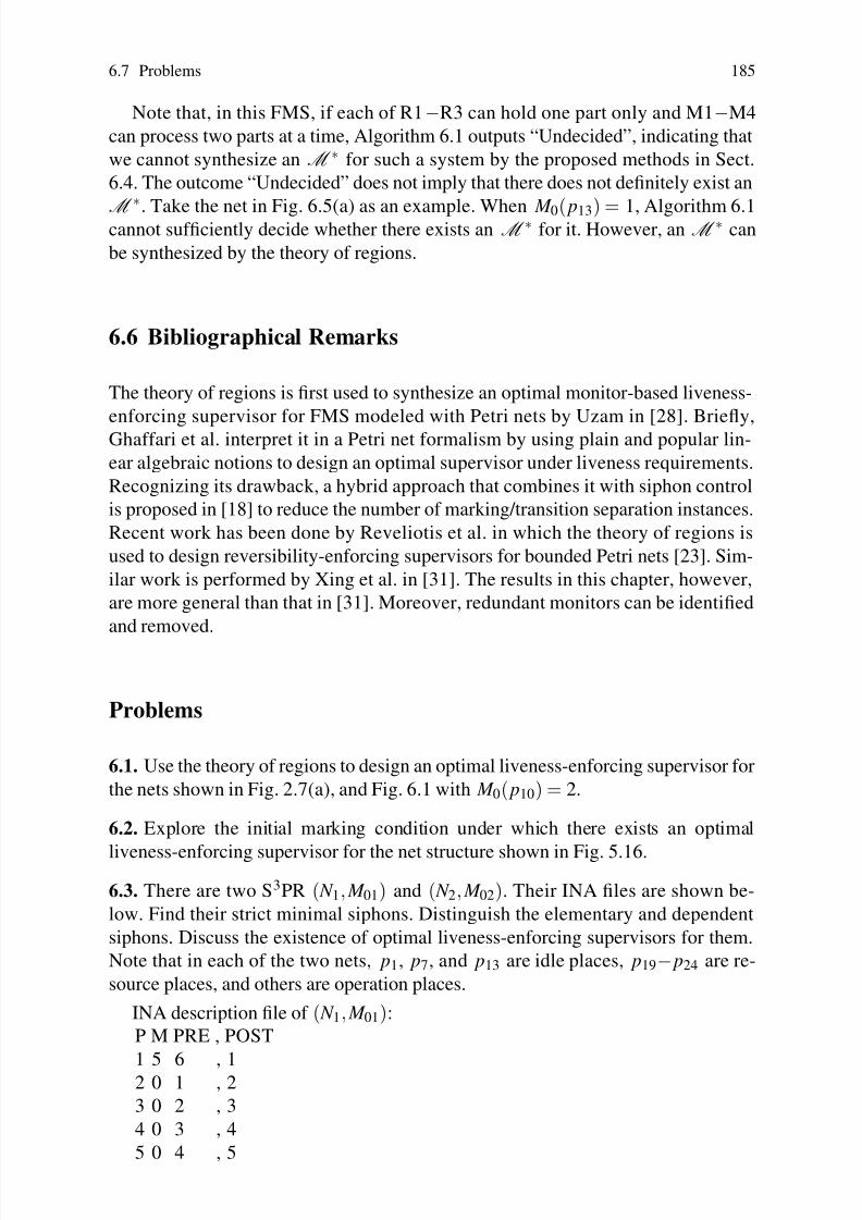
8/4/2019 Li Z., Zhou M. Deadlock Resolution in Automated Manufacturing Systems - A Novel Petri Net Approach
http://slidepdf.com/reader/full/li-z-zhou-m-deadlock-resolution-in-automated-manufacturing-systems-a-novel 198/249
6.7 Problems 185
Note that, in this FMS, if each of R1−R3 can hold one part only and M1−M4
can process two parts at a time, Algorithm 6.1 outputs “Undecided”, indicating that
we cannot synthesize an M ∗ for such a system by the proposed methods in Sect.
6.4. The outcome “Undecided” does not imply that there does not definitely exist an
M ∗. Take the net in Fig. 6.5(a) as an example. When M 0( p13) = 1, Algorithm 6.1cannot sufficiently decide whether there exists an M ∗ for it. However, an M ∗ can
be synthesized by the theory of regions.
6.6 Bibliographical Remarks
The theory of regions is first used to synthesize an optimal monitor-based liveness-
enforcing supervisor for FMS modeled with Petri nets by Uzam in [28]. Briefly,
Ghaffari et al. interpret it in a Petri net formalism by using plain and popular lin-
ear algebraic notions to design an optimal supervisor under liveness requirements.
Recognizing its drawback, a hybrid approach that combines it with siphon control
is proposed in [18] to reduce the number of marking/transition separation instances.
Recent work has been done by Reveliotis et al. in which the theory of regions is
used to design reversibility-enforcing supervisors for bounded Petri nets [23]. Sim-
ilar work is performed by Xing et al. in [31]. The results in this chapter, however,
are more general than that in [31]. Moreover, redundant monitors can be identified
and removed.
Problems
6.1. Use the theory of regions to design an optimal liveness-enforcing supervisor for
the nets shown in Fig. 2.7(a), and Fig. 6.1 with M 0( p10) = 2.
6.2. Explore the initial marking condition under which there exists an optimal
liveness-enforcing supervisor for the net structure shown in Fig. 5.16.
6.3. There are two S3PR ( N 1, M 01) and ( N 2, M 02). Their INA files are shown be-
low. Find their strict minimal siphons. Distinguish the elementary and dependent
siphons. Discuss the existence of optimal liveness-enforcing supervisors for them.
Note that in each of the two nets, p1, p7, and p13 are idle places, p19− p24 are re-
source places, and others are operation places.
INA description file of ( N 1, M 01):
P M PRE , POST
1 5 6 , 1
2 0 1 , 2
3 0 2 , 3
4 0 3 , 4
5 0 4 , 5
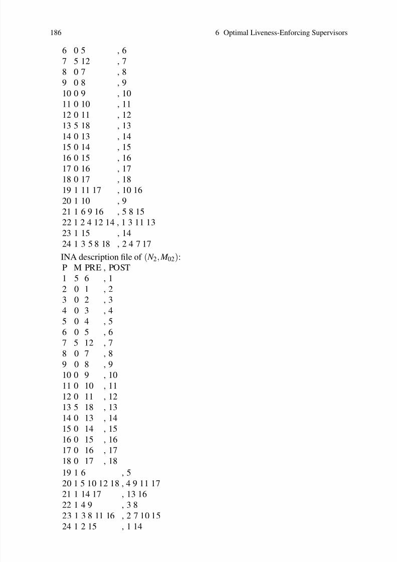
8/4/2019 Li Z., Zhou M. Deadlock Resolution in Automated Manufacturing Systems - A Novel Petri Net Approach
http://slidepdf.com/reader/full/li-z-zhou-m-deadlock-resolution-in-automated-manufacturing-systems-a-novel 199/249
186 6 Optimal Liveness-Enforcing Supervisors
6 0 5 , 6
7 5 12 , 7
8 0 7 , 8
9 0 8 , 9
10 0 9 , 10
11 0 10 , 11
12 0 11 , 12
13 5 18 , 13
14 0 13 , 14
15 0 14 , 15
16 0 15 , 16
17 0 16 , 17
18 0 17 , 18
19 1 11 17 , 10 16
20 1 10 , 9
21 1 6 9 16 , 5 8 15
22 1 2 4 12 14 , 1 3 11 13
23 1 15 , 14
24 1 3 5 8 18 , 2 4 7 17
INA description file of ( N 2, M 02):
P M PRE , POST
1 5 6 , 1
2 0 1 , 2
3 0 2 , 3
4 0 3 , 4
5 0 4 , 5
6 0 5 , 6
7 5 12 , 7
8 0 7 , 8
9 0 8 , 9
10 0 9 , 10
11 0 10 , 11
12 0 11 , 1213 5 18 , 13
14 0 13 , 14
15 0 14 , 15
16 0 15 , 16
17 0 16 , 17
18 0 17 , 18
19 1 6 , 5
20 1 5 10 12 18 , 4 9 11 17
21 1 14 17 , 13 1622 1 4 9 , 3 8
23 1 3 8 11 16 , 2 7 10 15
24 1 2 15 , 1 14
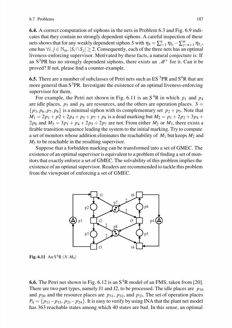
8/4/2019 Li Z., Zhou M. Deadlock Resolution in Automated Manufacturing Systems - A Novel Petri Net Approach
http://slidepdf.com/reader/full/li-z-zhou-m-deadlock-resolution-in-automated-manufacturing-systems-a-novel 200/249
6.7 Problems 187
6.4. A correct computation of siphons in the nets in Problem 6.3 and Fig. 6.9 indi-
cates that they contain no strongly dependent siphons. A careful inspection of these
nets shows that for any weakly dependent siphon S with ηS =∑ni=1ηSi
−∑m j=n+1ηS j
,
one has ∀i, j ∈Nm, |Si ∩S j| ≥ 2. Consequently, each of the three nets has an optimal
liveness-enforcing supervisor. Motivated by these facts, a natural conjecture is: If an S3PR has no strongly dependent siphons, there exists an M ∗ for it. Can it be
proved? If not, please find a counter-example.
6.5. There are a number of subclasses of Petri nets such as ES 3PR and S4R that are
more general than S3PR. Investigate the existence of an optimal liveness-enforcing
supervisor for them.
For example, the Petri net shown in Fig. 6.11 is an S4R in which p1 and p4
are idle places, p7 and p8 are resources, and the others are operation places. S =
p3, p6, p7, p8
is a minimal siphon with its complementary set p2 + p5. Note that
M 1 = 2 p1 + p2 + 2 p4 + p5 + p7 + p8 is a dead marking but M 2 = p1 + 2 p2 + 3 p4 +2 p8 and M 3 = 3 p1 + p4 + 2 p5 + 2 p7 are not. From either M 2 or M 3, there exists a
firable transition sequence leading the system to the initial marking. Try to compute
a set of monitors whose addition eliminates the reachability of M 1 but keeps M 2 and
M 3 to be reachable in the resulting supervisor.
Suppose that a forbidden marking can be transformed into a set of GMEC. The
existence of an optimal supervisor is equivalent to a problem of finding a set of mon-
itors that exactly enforce a set of GMEC. The solvability of this problem implies the
existence of an optimal supervisor. Readers are recommended to tackle this problem
from the viewpoint of enforcing a set of GMEC.
p 2 p 6
p 5p 3
p 7
p 4p 1
p 8
t 1 t 6
t 5
t 4t 3
t 2
2
2
2
2
Fig. 6.11 An S4R ( N , M 0)
6.6. The Petri net shown in Fig. 6.12 is an S4R model of an FMS, taken from [20].
There are two part types, namely J1 and J2, to be processed. The idle places are p10
and p20 and the resource places are p31, p32, and p33. The set of operation places
P A = p11− p15, p21− p24. It is easy to verify by using INA that the plant net model
has 363 reachable states among which 40 states are bad. In this sense, an optimal

8/4/2019 Li Z., Zhou M. Deadlock Resolution in Automated Manufacturing Systems - A Novel Petri Net Approach
http://slidepdf.com/reader/full/li-z-zhou-m-deadlock-resolution-in-automated-manufacturing-systems-a-novel 201/249
188 6 Optimal Liveness-Enforcing Supervisors
controlled system should have 323 reachable states. Try to use the theory of regions
to check the existence of an optimal liveness-enforcing supervisor for the plant net
model. Note that a finite-state automaton cannot always find a label-free Petri net
implementation.
p 1 0
p 1 5
p 1 4
t 7
t 6
p 1 2
p 1 3
t 3
p 3 1
t 2
t 4
t 5
p 1 1
t 1
2
p 2 4
t 1 3
p 2 2
p 2 3
t 1 0
t 9
t 1 1
t 1 2
p 2 1
t 8
p 2 0
2
4
32
p 3 2
p 3 3
R 1
R 3
R 2
2
Fig. 6.12 An S4R ( N , M 0)
Suppose that there does not exist an optimal monitor-based liveness-enforcing
supervisor given a plant net model. Develop an algorithm to find such a supervisor
Sup that there does not exist another supervisor Sup′ that is more permissive than
Sup. About this problem, the reader is referred to [29] in which a nearly optimal
supervisor is computed by an iterative deadlock state elimination method. However,
it is not formally proved that in a general case the proposed deadlock prevention
policy can always find the best supervisor when an optimal one does not exist.
References
1. Abdallah, I.B., ElMaraghy, H.A. (1998) Deadlock prevention and avoidance in FMS: A Petri
net based approach. International Journal of Advanced Manufacturing Technology, vol.14,
no.10, pp.704–715.
2. Badouel, E., Darondeau, P. (1998) Theory of regions. Lectures on Petri Nets I: Basic Models,
Lecture Notes in Computer Science, vol.1491, W. Reisig and G. Rozenberg (Eds.), pp.529–
586.3. Barkaoui, K., Lemaire, B. (1989) An effective characterization of minimal deadlocks and
traps in Petri nets based on graph theory. In Proc. 10th Int. Conf. on Application and Theory
of Petri Nets, pp.1–21.

8/4/2019 Li Z., Zhou M. Deadlock Resolution in Automated Manufacturing Systems - A Novel Petri Net Approach
http://slidepdf.com/reader/full/li-z-zhou-m-deadlock-resolution-in-automated-manufacturing-systems-a-novel 202/249
References 189
4. Barkaoui, K., Abdallah, I.B. (1994) An efficient deadlock avoidance control policy in FMS
using structural analysis of Petri nets. In Proc. IEEE Int. Conf. on Systems, Man, and Cyber-
netics, vol.1, pp.525–530.
5. Barkaoui, K., Abdallah, I.B. (1995) A deadlock prevention method for a class of FMS. In
Proc. IEEE Int. Conf. on Systems, Man, and Cybernetics, vol.5, pp.4119–4124.
6. Barkaoui, K., Abdallah, I.B. (1995) Deadlock avoidance in FMS based on structural theoryof Petri nets. In Proc. INRIA/IEEE Symposium on Emerging Technologies and Factory Au-
tomation, vol.2, pp.499–510.
7. Chu, F., Xie, X.L. (1997) Deadlock analysis of Petri nets using siphons and mathematical
programming. IEEE Transactions on Robotics and Automation, vol.13, no.6, pp.793–804.
8. Cormen, T.H., Leiserson, C.E., Rivest, R.L. (1992) Introduction to Algorithms. The MIT
Press/McGraw-Hill.
9. Darondeau, P. (2000) Region based synthesis of P/T-nets and its potential applications. In
Pro. 20th Int. Conf. on Applications and Theory of Petri Nets, Lecture Notes in Computer
Science, vol.1825, pp.16–23.
10. Ezpeleta, J, Colom, J.M., Martinez, J. (1995) A Petri net based deadlock prevention policy
for flexible manufacturing systems. IEEE Transactions on Robotics and Automation, vol.11,no.2, pp.173–184.
11. Ghaffari, A., Rezg, N., Xie, X.L. (2003) Design of a live and maximally permissive Petri
net controller using the theory of regions. IEEE Transactions on Robotics and Automation,
vol.19, no.1, pp.137–142.
12. Giua, A., DiCesare, F., Silva, M. (1992) Generalized mutual exclusion constraints on nets
with uncontrollable transitions. In Proc. IEEE Int. Conf. on Systems, Man, and Cybernetics,
vol.2, pp.974–979.
13. Huang, Y.S., Jeng, M.D., Xie, X.L., Chung, S.L. (2001) Deadlock prevention policy based on
Petri nets and siphons. International Journal of Production Research, vol.39, no.2, pp.283–
305.
14. Lawley, M.A., Reveliotis, S.A. (2001) Deadlock avoidance for sequential resource alloca-tion systems: Hard and easy cases. International Journal of Flexible Manufacturing Systems,
vol.13, no.4, pp.385–404.
15. Li, Z.W., Zhou, M.C. (2004) Elementary siphons of Petri nets and their application to dead-
lock prevention in flexible manufacturing systems. IEEE Transactions on Systems, Man, and
Cybernetics, Part A, vol.34, no.1, pp.38–51.
16. Li, Z.W., Zhou, M.C. (2006) Two-stage method for synthesizing liveness-enforcing super-
visors for flexible manufacturing systems using Petri nets. IEEE Transactions on Industrial
Informatics, vol.2, no.4, pp.313–325.
17. Li, Z.W., Liu, D. (2007) A correct minimal siphons extraction algorithm from a maximal
unmarked siphon of a Petri net. International Journal of Production Research, vol.45, no.9,
pp.2163–2167.18. Li, Z.W., Zhou, M.C., Jeng, M.D. (2008) A maximally permissive deadlock prevention policy
for FMS based on Petri net siphon control and the theory of regions. IEEE Transactions on
Automation Science and Engineering, vol.5, no.1, pp.182–188.
19. Lindo, Premier Optimization Modeling Tools, http://www.lindo.com/.
20. Park, J., Reveliotis, S.A. (2001) Deadlock avoidance in sequential resource allocation systems
with multiple resource acquisitions and flexible routings. IEEE Transactions on Automatic
Control, vol.46, no.10, pp.1572–1583.
21. Paton, K. (1969) An algorithm for finding a fundamental set of cycles of a graph. Communi-
cations of the ACM , vol.12, no.9, pp.514–518.
22. Ramadge, P., Wonham, W.M. (1989) The control of discrete event systems. Proceedings of
the IEEE , vol.77, no.1, pp.81–89.23. Reveliotis, S.A., Choi, J.Y. (2006) Designing reversibility-enforcing supervisors of polyno-
mial complexity for bounded Petri nets through the theory of regions. In Proc. 27th Int. Conf.
on Applications and Theory of Petri Nets and Other Models of Concurrency, Lecture Notes
in Computer Science, vol.4024, S. Donatelli and P. S. Thiagarajan (Eds.), pp.322–341.

8/4/2019 Li Z., Zhou M. Deadlock Resolution in Automated Manufacturing Systems - A Novel Petri Net Approach
http://slidepdf.com/reader/full/li-z-zhou-m-deadlock-resolution-in-automated-manufacturing-systems-a-novel 203/249
190 6 Optimal Liveness-Enforcing Supervisors
24. Sreenivas, R.S. (1997) On Commoner’s liveness theorem and supervisory policies that en-
force liveness in free-choice Petri nets. Systems Control Letters, vol.31, no.1, pp.41–48.
25. Sreenivas, R.S. (1997) On the existence of supervisory control policies that enforce liveness
in discrete-event dynamic systems modeled by controlled Petri nets. IEEE Transactions on
Automatic Control, vol.42, no.7, pp.928–945.
26. Sreenivas, R.S. (1999) On supervisory policies that enforce liveness in completely controlledPetri nets with directed cut-places and cut-transitions. IEEE Transactions on Automatic Con-
trol, vol.44, no.6, pp.1221–1225.
27. Starke, P.H. (2003) INA: Integrated Net Analyzer . http://www2.informatik.hu-berlin.de/ ∼starke/ina.html.
28. Uzam, M. (2002) An optimal deadlock prevention policy for flexible manufacturing systems
using Petri net models with resources and the theory of regions. International Journal of
Advanced Manufacturing Technology, vol.19, no.3, pp.192–208.
29. Uzam, M., Zhou, M.C. (2006) An improved iterative synthesis method for liveness enforcing
supervisors of flexible manufacturing systems. International Journal of Production Research,
vol.44, no.10, pp.1987–2030.
30. Uzam, M., Li, Z.W., Zhou, M.C. (2007) Identification and elimination of redundant controlplaces in Petri net based liveness enforcing supervisors of FMS. International Journal of
Advanced Manufacturing Technology, vol.35, no.1–2, pp.150–168.
31. Xing, K.Y., Hu, B.S. (2005) Optimal liveness Petri net controllers with minimal structures for
automated manufacturing systems. In Proc. IEEE Int. Conf. on Systems, Man and Cybernet-
ics, pp.282–287.

8/4/2019 Li Z., Zhou M. Deadlock Resolution in Automated Manufacturing Systems - A Novel Petri Net Approach
http://slidepdf.com/reader/full/li-z-zhou-m-deadlock-resolution-in-automated-manufacturing-systems-a-novel 204/249
Chapter 7
Comparison of Deadlock Prevention Policies
Abstract This chapter, through a typical case study, reviews and compares a vari-
ety of Petri net-based deadlock prevention policies reported in the literature. Their
comparison is done in terms of a resultant supervisor’s structural complexity, behav-
ior permissiveness, and computational complexity. This comparison study should
help engineers to choose a suitable method for their industrial application cases. It
is concluded that when behavior permissiveness is not a major concern, a policy
with polynomial complexity should be the best choice for industrial-size automated
systems. If the online computational cost is not a problem, an optimal deadlock
prevention policy should be the best choice of industrial engineers. The deadlock
prevention policies that use partial siphon enumeration achieve a good balance be-
tween the behavior permissiveness and computational complexity.
7.1 Introduction
Over the last two decades, a great deal of research has been focused on solving
deadlock problems in resource allocation systems such as computer communica-
tion systems, workflow systems, and flexible manufacturing systems, resulting in awide variety of approaches. Deadlock prevention is considered to be a well-defined
problem in discrete-event systems literature, which is usually achieved by using an
off-line computational mechanism to control the request for resources to ensure that
deadlocks never occur. The goal of a deadlock prevention approach is to impose
constraints on a system to prevent it from reaching deadlock states. In this case,
the computation is carried out off-line in a static way and once the control policy
is established, the system can no longer reach undesirable deadlock states. A ma-
jor advantage of deadlock prevention algorithms is that they require no run-time
cost since problems are solved in system design and planning stages. Due to its ad-vantage over deadlock detection and recovery, and deadlock avoidance, deadlock
prevention based on a Petri net formalism has received an enormous amount of at-
tention in the literature. This chapter intends, through a typical case study, to review
191

8/4/2019 Li Z., Zhou M. Deadlock Resolution in Automated Manufacturing Systems - A Novel Petri Net Approach
http://slidepdf.com/reader/full/li-z-zhou-m-deadlock-resolution-in-automated-manufacturing-systems-a-novel 205/249
192 7 Comparison of Deadlock Prevention Policies
and compare a variety of Petri net-based deadlock prevention policies reported in
the literature. Their comparison is done in terms of structural complexity, behavior
permissiveness, and computational complexity. This comparison study should help
engineers to choose a suitable method for their industrial application cases.
7.2 Applications of Deadlock Prevention Methods to a Case
Study
The deadlock prevention policies that are investigated in this chapter are shown in
Table 7.1. This section presents the supervisors for the FMS example in Sect. 5.4 by
these deadlock prevention policies.
Table 7.1 Deadlock prevention policies
Researchers Policy notation Applicable nets
Abdallah and ElMaraghy [1] AE-policy S4R
Barkaoui and Abdallah [2] B1-policy G-system
Barkaoui et al. [5] B2-policy S3PR
Piroddi et al. [77] P-policy Petri nets
Ezpeleta et al. [19] E-policy S3PR
Huang et al. [36] H1-policy S3PR
Huang [38] H2-policy S3PR
Li and Zhou [57] L1-policy S3PR
Li et al. [63] L2-policy S3PR
Li and Zhou [61] L3-policy S3PR
Park and Reveliotis [73] PR-policy S4R
Tricas et al. [89] T-policy S4R
Uzam [92] U1-policy Petri nets
Uzam and Zhou [95] U2-policy Petri nets
Xing and Hu [101] X-policy S3PR
The Petri net model of an FMS depicted in Fig. 5.8 is used to conduct the casestudy. It contains 18 strict minimal siphons shown in Table 7.2 again to facilitate
the reader’s understanding of these policies where a dependent one is marked with
a star. Note that in the following tables in this chapter, monitor V Sior V i does not
necessarily correspond to siphon Si since some policies do not need to explicitly
control the siphons in Table 7.2.
7.2.1 Combination of Deadlock Prevention and Avoidance
Abdallah and ElMaraghy [1] propose a deadlock control method, AE-policy for
short, for S4R nets that are more general than S3PR. This policy combines deadlock

8/4/2019 Li Z., Zhou M. Deadlock Resolution in Automated Manufacturing Systems - A Novel Petri Net Approach
http://slidepdf.com/reader/full/li-z-zhou-m-deadlock-resolution-in-automated-manufacturing-systems-a-novel 206/249
7.2 Applications of Deadlock Prevention Methods to a Case Study 193
Table 7.2 Strict minimal siphons in the case study (“*” means a dependent siphons after S1, S4,
S10, and S16−S18 are selected as elementary ones)
S Places S Places
S1 p10, p18, p22, p26 S∗2 p4, p10, p15, p20− p26
S∗3 p4, p10, p16, p21, p22, p24, p25, p26 S4 p4, p10, p17, p21, p22, p24, p26
S∗5 p4, p9, p13, p15, p20, p21, p23− p26 S∗
6 p4, p9, p13, p16, p21, p24, p25, p26
S∗7 p4, p9, p13, p17, p21, p24, p26 S∗
8 p4, p9, p12, p15, p20, p21, p23, p24, p25
S∗9 p4, p9, p12, p16, p21, p24, p25 S10 p4, p9, p12, p17, p21, p24
S∗11 p2, p4, p8, p10, p15, p20− p23, p25, p26 S∗
12 p2, p4, p8, p13, p15, p20, p21, p23, p25, p26
S∗13 p2, p4, p8, p10, p16, p21, p22, p25, p26 S∗
14 p2, p4, p8, p13, p16, p21, p25, p26
S∗15 p2, p4, p8, p10, p17, p21, p22, p26 S16 p2, p4, p8, p13, p17, p21, p26
S17 p2, p4, p8, p12, p15, p20, p21, p23, p25 S18 p2, p4, p8, p12, p16, p21, p25
prevention and avoidance strategies. It consists of two stages. First, a monitor V S is
added for each strict minimal siphon S in a plant Petri net model ( N , M 0) by the en-forcement that [S]∪V S is the support of a P-semiflow of the augmented net system
( N α , M α 0 ), where M α 0 (V S) = M 0(S) − 1. In some cases, the first stage of AE-policy
cannot eliminate deadlock states completely. When the occurrences of deadlocks
remain possible in ( N α , M α 0 ), an on-line controller that uses a dynamic resource al-
location policy is employed such that the evolution of ( N α , M α 0 ) can never enter an
unsafe state that inevitably leads the system to deadlock.
For the net system in Fig. 5.8, 18 monitors are added due to AE-policy and their
initial marking, presets and postsets are shown in Table 7.3.
Table 7.3 Monitors added using AE-policy
V S M α 0 (·) Preset Postset V S M α 0 (·) Preset Postset
V S12 t 10,t 16 t 9, t 15 V S2
10 t 5, t 10, t 13, t 19 t 1, t 11,t 15
V S37 t 5,t 10,t 13,t 18 t 3, t 7, t 11, t 15 V S4
5 t 5, t 10, t 13, t 17 t 3, t 8, t 11,t 15
V S59 t 4,t 9,t 13,t 19 t 1, t 11, t 16 V S6
6 t 4, t 9, t 13, t 18 t 3, t 7, t 11,t 16
V S74 t 4,t 9,t 13,t 17 t 3, t 8, t 11, t 16 V S8
7 t 4, t 8, t 13, t 19 t 1, t 11,t 17
V S94 t 4,t 8,t 13,t 18 t 3, t 7, t 11, t 17 V S10
2 t 4, t 13 t 3, t 11
V S118 t 3,t 10,t 19 t 1, t 15 V S12
7 t 3, t 9, t 19 t 1, t 16
V S13 5 t 10,t 18 t 7, t 15 V S14 4 t 9, t 18 t 7, t 16V S15
3 t 10,t 17 t 8, t 15 V S162 t 9, t 17 t 8, t 16
V S175 t 3,t 8,t 19 t 1, t 17 V S18
2 t 8, t 18 t 7, t 17
After the monitors are added, the augmented net system ( N α , M α 0 ) contains dead-
locks. As a result, the second stage is necessary for this example. Similar to AE-
policy, a hybrid (prevention and avoidance) deadlock control approach is proposed
by Barkaoui et al. [3].
Remark 7.1. The number of the monitors added in the first stage is equal to that
of the strict minimal siphons in a plant model. Unfortunately, the number of such
siphons in an S3PR is theoretically exponential with respect to its size. This im-
plies that in the first stage of AE-policy the number of the additional monitors is
exponential with respect to the size of a plant model.

8/4/2019 Li Z., Zhou M. Deadlock Resolution in Automated Manufacturing Systems - A Novel Petri Net Approach
http://slidepdf.com/reader/full/li-z-zhou-m-deadlock-resolution-in-automated-manufacturing-systems-a-novel 207/249
194 7 Comparison of Deadlock Prevention Policies
Remark 7.2. In AE-policy, the existence of deadlocks in ( N α , M α 0 ) is confirmed by
verifying the presence of strict minimal siphons in it. This means that one has to
find them in ( N α , M α 0 ), which becomes more time-consuming if in the first stage
the concept of elementary siphons is not adopted. However, whether the second
stage of AE-policy is necessary can be decided by pure structural analysis as statedin Chap. 6.
Remark 7.3. Chapter 6 also presents some conditions under which the first stage
of this policy leads to an optimal liveness-enforcing supervisor. Furthermore, when
the second stage is necessary, the concept of elementary siphons can be applied in
the first stage, leading to a structurally simple intermediate Petri net. This would
facilitate the siphon computation in the second stage. For the example investigated
in this chapter, the first stage needs six monitors that are added for the elementary
siphons with each siphon control variable being one. In this case, the dependent
siphons in the plant model are implicitly controlled.
7.2.2 Modification of Initial Markings of Monitors
Barkaoui and Abdallah [2] develop a deadlock prevention method, called B1-policy
for short, for S3PR nets, which consists of two stages. The strict minimal siphons in
a plant S3PR are distinguished by basic strict minimal siphons and dependent strict
minimal siphons. Its first stage is identical to that of AE-policy. When the deadlock-freedom or liveness in the augmented net system is not guaranteed, the second stage
tries to modify the initial markings of the additional monitors added for dependent
strict minimal siphons according to the proposed rules. Table 7.4 shows the monitors
due to this policy for the example.
Table 7.4 Monitors added using B1-policy
V S M α 0 (·) Preset Postset V S M α 0 (·) Preset Postset
V S12 t 10,t 16 t 9, t 15 V S2
9 t 5, t 10, t 13, t 19 t 1, t 11,t 15
V S3 6 t 5,t 10,t 13,t 18 t 3, t 7, t 11, t 15 V S4 5 t 5, t 10, t 13, t 17 t 3, t 8, t 11,t 15
V S58 t 4,t 9,t 13,t 19 t 1, t 11, t 16 V S6
5 t 4, t 9, t 13, t 18 t 3, t 7, t 11,t 16
V S73 t 4,t 9,t 13,t 17 t 3, t 8, t 11, t 16 V S8
6 t 4, t 8, t 13, t 19 t 1, t 11,t 17
V S93 t 4,t 8,t 13,t 18 t 3, t 7, t 11, t 17 V S10
2 t 4, t 13 t 3, t 11
V S118 t 3,t 10,t 19 t 1, t 15 V S12
6 t 3, t 9, t 19 t 1, t 16
V S135 t 10,t 18 t 7, t 15 V S14
3 t 9, t 18 t 7, t 16
V S153 t 10,t 17 t 8, t 15 V S16
2 t 9, t 17 t 8, t 16
V S175 t 3,t 8,t 19 t 1, t 17 V S18
2 t 8, t 18 t 7, t 17
Remark 7.4. Note that B1-policy may be problematic since it cannot lead to aliveness-enforcing supervisor for this example. This policy needs further investi-
gation. Similar to AE-policy, the first stage of B1-policy can lead to an optimal
liveness-enforcing supervisor under some conditions as presented in Chap. 6.

8/4/2019 Li Z., Zhou M. Deadlock Resolution in Automated Manufacturing Systems - A Novel Petri Net Approach
http://slidepdf.com/reader/full/li-z-zhou-m-deadlock-resolution-in-automated-manufacturing-systems-a-novel 208/249
7.2 Applications of Deadlock Prevention Methods to a Case Study 195
7.2.3 Deadlock Prevention via Proper Configuration of Initial
Markings
The places in a manufacturing-oriented Petri net model are usually distinguished
by idle, operation, and resource places [15], as done in augmented marked graphs[13], S3PR [19], L-S3PR [20], S4R [1], S4PR [89], WS3PSR [87], PNR [44], RCN-
merged nets [43], ERCN-merged nets [100], ERCN∗-merged nets [45], S3PGR2
[73], G-task [5], and G-system [106]. Given a system with a fixed resource capacity,
contrary to the monitor-based deadlock control methods, the Petri net model can
be built by properly configuring the initial markings of its idle places such that the
model itself is live. This idea can be traced back to the seminal works of Zhou,
DiCesare, and Jeng in 1990s [40, 41, 103–105]. In the last decade, a fair amount
of work in this direction has been done by Jeng and Xie [13, 43–45] in which the
liveness of a plant model is tied to the non-existence of emptiable siphons. Chao [11]develops a maximal class of Petri nets, called non-virtual (NV) nets. An NV net is
live iff there is no siphon that can become empty.
Motivated by the work mentioned above, Barkaoui et al. [5,106] propose a dead-
lock prevention method, called B2-policy for short. It can derive a set of expressions
about the initial markings of the idle and resource places in a G-system, under which
all siphons are max-controlled and the net system itself is live or non-blocking. Since
S3PR nets are a subclass of G-systems, B2-policy can be applied to an S3PR.
For an S3PR ( N , M 0), B2-policy first computes Π , the set of strict minimal
siphons in N . ∀S ∈ Π , its controllability is ensured by constructing a P-invariant zS such that zT
S M 0 > 0 and || zS||+ ⊆ S. zS is computed as follows:
zS = gS −θ ShS,
gS = ∑r ∈S R I r ,
hS = ∑ p∈[S] I p,
θ S = max p∈[S]∩||hS ||gS( p),
where I r is the minimal P-semiflow associated with resource place r , [S] is the com-
plementary set of siphon S, and I p is the minimal P-semiflow associated with oper-
ation place p. I p’s support consists of idle and operation places but does not contain
resource places.Since every operation needs only one resource to perform, it is easy to prove that
in an S3PR ∀S ∈Π , θ S = 1. For example, S1 = p10, p18, p22, p26 is a siphon in our
case study net. We have
I p22= p22 + p10 + p19,
I p26= p26 + p13 + p18,
gS1= I p22
+ I p26= p22 + p10 + p19 + p26 + p13 + p18,
[S1] = p13, p19,
hS1= ∑
13i=5 pi +∑19
i=14 pi,
zS1
= p22 + p26
−∑
9
i=5
pi
−∑
12
i=11
pi
−∑
17
i=14
pi.
Considering that ∀ p ∈ P A, M 0( p) = 0, we have that S1 is controlled if zT S1
M 0 > 0,
i.e., M 0( p22) + M 0( p26) − M 0( p5) − M 0( p14) > 0. In summary, the controllability

8/4/2019 Li Z., Zhou M. Deadlock Resolution in Automated Manufacturing Systems - A Novel Petri Net Approach
http://slidepdf.com/reader/full/li-z-zhou-m-deadlock-resolution-in-automated-manufacturing-systems-a-novel 209/249
196 7 Comparison of Deadlock Prevention Policies
of the 18 strict minimal siphons is shown by (7.1)−(7.18), where for economy of
space, we use µ i to denote M 0( pi) where there is no confusion.
S1
: µ 22
+µ 26 −
µ 5 −
µ 14> 0, (7.1)
S2 : µ 20 +µ 21 +µ 22 +µ 23 +µ 24 +µ 25 +µ 26 −µ 1 −µ 5 −µ 14 > 0, (7.2)
S3 :µ 21 +µ 22 +µ 24 +µ 25 +µ 26 −µ 1 −µ 5 −µ 14 > 0, (7.3)
S4 : µ 21 +µ 22 +µ 24 +µ 26 −µ 1 −µ 5 −µ 14 > 0, (7.4)
S5 : µ 20 +µ 21 +µ 23 +µ 24 +µ 25 +µ 26 −µ 1 −µ 5 −µ 14 > 0, (7.5)
S6 : µ 21 +µ 24 +µ 25 +µ 26 −µ 1 −µ 5 −µ 14 > 0, (7.6)
S7 : µ 21 +µ 24 +µ 26 −µ 1 −µ 5 −µ 14 > 0, (7.7)
S8 : µ 20 +µ 21 +µ 23 +µ 24 +µ 25
−µ 1
−µ 5
−µ 14 > 0, (7.8)
S9 : µ 21 +µ 24 +µ 25 −µ 1 −µ 5 −µ 14 > 0, (7.9)
S10 : µ 21 +µ 24 −µ 1 −µ 5 > 0, (7.10)
S11 : µ 20 +µ 21 +µ 22 +µ 23 +µ 25 +µ 26 −µ 5 −µ 14 > 0, (7.11)
S12 : µ 20 +µ 21 +µ 23 +µ 25 +µ 26 −µ 5 −µ 14 > 0, (7.12)
S13 : µ 21 +µ 22 +µ 25 +µ 26 −µ 5 −µ 14 > 0, (7.13)
S14 : µ 21 +µ 25 +µ 26 −µ 5 −µ 14 > 0, (7.14)
S15 : µ 21 +µ 22 +µ 26 −µ 5 −µ 14 > 0, (7.15)
S16 : µ 21 +µ 26 −µ 5 −µ 14 > 0, (7.16)S17 : µ 20 +µ 21 +µ 23 +µ 25 −µ 5 −µ 14 > 0, (7.17)
S18 : µ 21 +µ 25 −µ 5 −µ 14 > 0. (7.18)
When each of the places modeling robots contains one token and each of the
places representing machine tools has two tokens, the initial marking of idle places
in this example, which satisfies (7.1)−(7.18), is M 0( p1) = M 0( p5) = M 0( p14) = 1.
As a result, the live initial marking derived by B2-policy is M 0 = p1 + p5 + p14 + p20 + p21 + p22 + 2 p23 + 2 p24 + 2 p25 + 2 p26. The number of reachable states under
this marking is 166.Similar to B2-policy, the live initial marking configuration approaches proposed
by Chu, Xie, and Jeng [13, 43, 44, 100] fall under this class of deadlock prevention
policies.
Remark 7.5. Although B2-policy does not need to add monitors to the original
plant net model, the permissive behavior in the controlled system is considerably
restricted. Specifically, the maximally permissive supervisor of this example has
21,581 reachable states as seen in the next subsection. B2-policy, however, only
leads to 166 reachable states. That is to say, only 0.77% of maximally permissivebehavior is preserved. We can conclude that this policy is rather conservative com-
pared with the others.

8/4/2019 Li Z., Zhou M. Deadlock Resolution in Automated Manufacturing Systems - A Novel Petri Net Approach
http://slidepdf.com/reader/full/li-z-zhou-m-deadlock-resolution-in-automated-manufacturing-systems-a-novel 210/249
7.2 Applications of Deadlock Prevention Methods to a Case Study 197
Remark 7.6. The number of liveness requirement constraints derived from B2-
policy is equal to that of the strict minimal siphons in an S3PR. As a result, this
number grows rapidly and in the worst case grows exponentially with respect to the
size of a net model. However, there may exist redundant liveness requirement con-
straints whose removal does not influence the liveness condition. For example, thetruth of (7.16) immediately leads to that of (7.15) due to µ 22 > 0 ( M 0( p22) > 0).
Specifically, (7.1), (7.7)−(7.10), (7.16), and (7.18) are essential for the example and
then the others become redundant with respect to them.
7.2.4 A Selective Siphon Control Policy
The deadlock prevention policy, called P-policy for short, proposed by Piroddi et
al. in [77] is performed in an iterative way. At each step, it needs the complete
siphon enumeration. Siphons are divided into essential and dominated ones. The
controllability of an essential siphon implies that of its dominated siphons. An es-
sential siphon is distinguished by solving a set-covering problem that is known to
be NP-hard. It is shown that in general P-policy cannot lead to an optimal liveness-
enforcing supervisor. For the Petri net example, however, it gives an optimal super-
visor whose corresponding optimal controlled system has 21,581 reachable states.
The monitors are shown in Table 7.5.
Table 7.5 Monitors added using P-policy
V S M α 0 (·) Preset Postset
V S12 t 10,t 16 t 9,t 15
V S25 t 5,t 10,t 13,t 17 t 3,t 8,t 11,t 15
V S32 t 4,t 13 t 3,t 11
V S42 t 9,t 17 t 8,t 16
V S52 t 8,t 18 t 7,t 17
V S65 t 3,t 8,t 19 t 1,t 17
V S73 t 10,t 17 t 8,t 15
V S8 5 2t 8, t 18 2t 7, t 16V S9
17 t 3,t 5,t 8,2t 10, t 17,2t 19 2t 1, t 9,2t 15,t 18
V S1012 3t 8, t 10,2t 18 4t 7,2t 15
V S1127 t 3,2t 5, t 8,3t 10,t 13,t 18,2t 19 3t 1, t 9, t 11,3t 15
V S1227 t 3,2t 5, t 9,2t 10,t 13,t 17,3t 19 3t 1, t 11,3t 15,t 18
V S138 t 5,2t 8, t 13, t 18 t 3,2t 7, t 11, t 15
Remark 7.7. At each iterative step, P-policy requires:
1. The complete enumeration of all minimal siphons.2. The generation of all dominated markings.
3. The solution of a set-covering problem.

8/4/2019 Li Z., Zhou M. Deadlock Resolution in Automated Manufacturing Systems - A Novel Petri Net Approach
http://slidepdf.com/reader/full/li-z-zhou-m-deadlock-resolution-in-automated-manufacturing-systems-a-novel 211/249
198 7 Comparison of Deadlock Prevention Policies
In theory, the computational complexity of each task mentioned above is expo-
nential with respect to the size of a Petri net. However, it is claimed in [77] that:
1. An efficient siphon computation is proposed in [16] that can deal with a Petri net
with more than 2
×107 strict minimal siphons in a reasonable time.
2. The dominated markings can be found by solving an integer LPP whose size isusually very small or zero if only few essential siphons are found.
3. In practice, the set-covering problem is extremely small, and can be efficiently
solved by using a mixed-integer-programming (MIP) solver.
P-policy assumes that the original Petri nets are ordinary. In some iterative step,
the intermediate nets may become generalized. In this case, an intermediate net is
transformed into an ordinary [47] or PT-ordinary one [39]. Then siphon control is
performed. Finally, an inverse transformation is necessary.
7.2.5 Deadlock Prevention by Complete Siphon Enumeration
The work by Ezpeleta et al. [19] is usually considered to be the first one that designs
monitor-based liveness-enforcing supervisors for FMS via the structural analysis of
Petri nets. Their deadlock prevention approach, E-policy for short, first computes Π ,the set of strict minimal siphons in an S3PR ( N , M 0). Then, ∀S ∈Π , a monitor V S is
added such that any output arc of V S points to the source transitions of the plant net
model, which ensures the non-existence of emptiable strict minimal siphons in theaugmented net system ( N α , M α 0 ) and leads to a liveness-enforcing supervisor. Table
7.6 shows the monitors due to this policy for the example. The resultant controlled
system has 6,287 reachable states with 18 monitors and 106 arcs.
Table 7.6 Monitors added using E-policy
V S M α 0 (·) Preset Postset V S M α 0 (·) Preset Postset
V S12 t 2,t 10,t 16 t 1, t 15 V S2
2 t 2, t 8, t 18 t 1, t 15
V S3
5 t 3,t 8,t 19 t 1, t 15 V S4
2 t 4, t 7, t 13 t 1, t 11
V S54 t 4,t 8,t 13,t 18 t 1, t 11, t 15 V S6
7 t 4, t 8, t 13, t 19 t 1, t 11,t 15
V S72 t 2,t 9,t 17 t 1, t 15 V S8
4 t 2, t 9, t 18 t 1, t 15
V S97 t 3,t 9,t 19 t 1, t 15 V S10
4 t 4, t 9, t 13, t 17 t 1, t 11,t 15
V S116 t 4,t 9,t 13,t 18 t 1, t 11, t 15 V S12
9 t 4, t 9, t 13, t 19 t 1, t 11,t 15
V S133 t 2,t 10,t 17 t 1, t 15 V S14
5 t 2, t 10, t 18 t 1, t 15
V S158 t 3,t 10,t 19 t 1, t 15 V S16
5 t 5, t 10, t 13, t 17 t 1, t 11,t 15
V S177 t 5,t 10,t 13,t 18 t 1, t 11, t 15 V S18
10 t 5, t 10, t 13, t 19 t 1, t 11,t 15
Remark 7.8. As is gradually recognized, E-policy suffers from a number of prob-
lems: structural complexity, behavior permissiveness, and computational complex-
ity. First of all, the number of additional monitors is equal to that of strict min-
imal siphons. That is to say, the structural complexity of the supervisor is expo-
nential with respect to the size of a plant net model. Second, this policy is rather

8/4/2019 Li Z., Zhou M. Deadlock Resolution in Automated Manufacturing Systems - A Novel Petri Net Approach
http://slidepdf.com/reader/full/li-z-zhou-m-deadlock-resolution-in-automated-manufacturing-systems-a-novel 212/249
7.2 Applications of Deadlock Prevention Methods to a Case Study 199
conservative. The supervisor resulting from E-policy for the example leads only
to 6,287/21,581 = 29.13% of maximally permissive behavior. Finally, it needs
complete siphon enumeration whose computation is time-consuming or impossi-
ble when the size of a plant is large. The subsequent deadlock control policies in the
literature aim to address these problems. Remark 7.9. It can be verified that some additional monitors in the controlled system
obtained by E-policy can be removed, while the liveness of the resultant net system
is preserved. Before the development of elementary siphons, fortunately, there is
an established tool inside Petri net theory, which can be used to remove redundant
places from a Petri net. These redundant places are called implicit places [32,78,85],
which have the property that their addition to or removal from a net system does
not change its behavior, i.e., an implicit place is redundant from the viewpoint of
system behavior. However, the condition to decide the implicitness of a monitor in
a net supervisor seems more difficult to meet than the one based on the elementarysiphon theory (a formal proof has not been found yet). That is to say, an additional
monitor can be removed by the elementary siphon-based methodology, but it does
not satisfy the condition of an implicit place developed in [78] and [85].
7.2.6 Two-Stage Deadlock Control
As is well known, the number of siphons in a Petri net grows rapidly and in theworst case grows exponentially with respect to its size. In theory, the number of
strict minimal siphons in an S3PR is also exponential with respect to its size. Hence,
their computation is expensive. Motivated by this well-recognized fact, Huang et
al. [36] propose a two-stage deadlock prevention policy, called H1-policy for short,
in which the complete siphon enumeration of a plant S3PR model is avoided.
H1-policy proceeds in an iterative way. At each step, the MIP-based deadlock
detection method that is first proposed in [13] is used to find a maximal emptiable
siphon in an S3PR ( N , M 0), from which a strict minimal siphon, denoted by S, is de-
rived. A monitor V S is added for S by the enforcement that [S]∪V S is the support of a P-semiflow of the augmented net system, as done in AE-policy. The siphon iden-
tification and monitor addition are performed iteratively until no siphons in ( N , M 0)can be emptied. Then, the first stage terminates. This termination leads to an aug-
mented net system ( N α , M α 0 ).
The existence of deadlocks in ( N α , M α 0 ) is verified by computing its strict mini-
mal siphons, as done in AE-policy and B1-policy. If ( N α , M α 0 ) has deadlock states,
the second stage is initiated. Similarly, the MIP-based deadlock detection method is
used to find a strict minimal siphon. Then a monitor is added to make it controlled.
However, the siphon control method in the second stage of H1-policy is different
from the one in the first. Any output arc of the monitors added in the second stage
points to the source transitions of the plant model, as done in E-policy. Since the
monitors added in the second stage cannot lead to problematic siphons any more,
the second stage can converge rapidly with respect to the elimination of deadlock

8/4/2019 Li Z., Zhou M. Deadlock Resolution in Automated Manufacturing Systems - A Novel Petri Net Approach
http://slidepdf.com/reader/full/li-z-zhou-m-deadlock-resolution-in-automated-manufacturing-systems-a-novel 213/249
200 7 Comparison of Deadlock Prevention Policies
states. Note that a siphon is said to be problematic if its insufficient markedness
(being empty in the case of ordinary Petri nets) is tied to a deadlock.
For the example, as shown in Table 7.7, H1-policy adds 15 monitors in the first
stage and only one monitor in the second stage, which result in a liveness-enforcing
supervisor, leading to 12,656 reachable states in the controlled system [58]. Notethat V S∗ is added for siphon S∗ = p10, p16, p22, p25, p26,V S16,V S18
in the second
stage.
Table 7.7 Monitors added using H1-policy
V S M α 0 (·) Preset Postset V S M α 0 (·) Preset Postset
V S12 t 10,t 16 t 9,t 15 V S4
5 t 5,t 10, t 13, t 17 t 3, t 8, t 11, t 15
V S66 t 4,t 9,t 13,t 18 t 3,t 7,t 11, t 16 V S7
4 t 4,t 9,t 13, t 17 t 3, t 8, t 11, t 16
V S87 t 4,t 8,t 13,t 19 t 1,t 11, t 17 V S9
4 t 4,t 8,t 13, t 18 t 3, t 7, t 11, t 17
V S10 2 t 4,t 13 t 3,t 11 V S11 8 t 3,t 10, t 19 t 1, t 15V S12
7 t 3,t 9,t 19 t 1,t 16 V S135 t 10, t 18 t 7, t 15
V S144 t 9,t 18 t 7,t 16 V S15
3 t 10, t 17 t 8, t 15
V S162 t 9,t 17 t 8,t 16 V S17
5 t 3,t 8,t 19 t 1, t 17
V S182 t 8,t 18 t 7,t 17 V S∗ 7 t 2,t 5,2t 10,2t 17 2t 1,2t 15
Remark 7.10. H1-policy is the first one that does not need the complete siphon enu-
meration, which can lead to more permissive behavior than E-policy. It is worthy to
note that the permissive behavior of the resultant supervisor depends on the siphons
controlled in the second stage. This is to say, selecting different siphons in the sec-ond stage to control may lead to the supervisors with different permissive behavior,
as shown in the next subsection.
Remark 7.11. For an S3PR, the second stage of H1-policy in general leads to a gen-
eralized Petri net supervisor, whose liveness is ensured by the max-controllability
of its siphons. Furthermore, it is clear that under some conditions the first stage of
H1-policy can lead to an optimal liveness-enforcing supervisor. These conditions,
for example, include the absence of dependent siphons in an S3PR plant model.
7.2.7 Two-Stage Deadlock Control with Elementary Siphons
Recognizing the possible existence of dependent siphons in a Petri net model and
their role in deadlock prevention, Huang [38] proposes a deadlock prevention pol-
icy, called H2-policy for short, for S3PR nets, which is an improved version of H1-
policy. The major difference of the two policies lies in their first stages. The first
stage of H2-policy finds the set of elementary siphons in an S 3PR net model pro-
vided that all strict minimal siphons are known. Then, a monitor is added for each
elementary siphon. Compared with H1-policy, this implies that fewer monitors are
needed in the first stage of H2-policy. Table 7.8 shows the monitors due to H2-policy
for the example.

8/4/2019 Li Z., Zhou M. Deadlock Resolution in Automated Manufacturing Systems - A Novel Petri Net Approach
http://slidepdf.com/reader/full/li-z-zhou-m-deadlock-resolution-in-automated-manufacturing-systems-a-novel 214/249
7.2 Applications of Deadlock Prevention Methods to a Case Study 201
In Table 7.8, V S1, V S4
, V S10, and V S16
−V S18are the monitors added in the first stage.
This is not surprising since there are only six elementary siphons in the example. As
in H1-policy, the second stage of H2-policy adds one monitor only. The supervisor
due to the additional monitors in Table 7.8 leads to 16,425 reachable states. The
permissive behavior of the two supervisors resulting from H1- and H2-policies isdifferent. This is caused by the fact that the siphon controlled in the second stage of
H1-policy is different from the one of H2-policy.
Table 7.8 Monitors added using H2-policy
V S M α 0 (·) Preset Postset V S M α 0 (·) Preset Postset
V S12 t 10,t 16 t 9, t 15 V S4
5 t 5, t 10, t 13, t 17 t 3, t 8, t 11,t 15
V S102 t 4,t 13 t 3, t 11 V S16
2 t 9, t 17 t 8, t 16
V S175 t 3,t 8,t 19 t 1, t 17 V S18
2 t 8, t 18 t 7, t 17
V S∗ 8 2t 2,2t 10,3t 18 2t 1,3t 15
Remark 7.12. Although H2-policy in general can lead to a structurally simple su-
pervisor by considering the existence of elementary siphons in a plant model, the
complete siphon enumeration becomes necessary again, which increases the com-
putational complexity of this policy. However, the first stage of H2-policy can be
improved, avoiding complete siphon enumeration, by the following steps:
1. Find a maximal unmarked siphon by the MIP-based deadlock detection ap-
proach, from which a strict minimal siphon S is derived.
2. If S is elementary, add V S for it; otherwise, check the controllability of S. If it is
not controlled, add a monitor for it.
3. Repeat the above two steps until all siphons in ( N , M 0) are controlled.
Such an improved H2-policy has the same computational complexity with H1-
policy, but in general it leads to a supervisor with less additional monitors.
Remark 7.13. In theory, it cannot be claimed that H2-policy is more permissive than
H1-policy although it is true for the example. The permissive behavior of the super-visor due to H1(H2)-policy depends on the siphons controlled in its second stage.
That is to say, if the siphons controlled in the second stage are identical, the resultant
supervisors lead to the same permissive behavior.
7.2.8 A Policy Based on Elementary Siphons
According to E-policy, the number of additional monitors in the supervisor of an
S3PR is, in theory, exponential with respect to its size. That is to say, E-policy
needs too many monitors when the size of a plant is large. To address this issue,
Li and Zhou propose the concept of elementary and redundant siphons [57]. Redun-
dant siphons are later renamed as dependent siphons [62]. In an S 3PR, a dependent

8/4/2019 Li Z., Zhou M. Deadlock Resolution in Automated Manufacturing Systems - A Novel Petri Net Approach
http://slidepdf.com/reader/full/li-z-zhou-m-deadlock-resolution-in-automated-manufacturing-systems-a-novel 215/249
202 7 Comparison of Deadlock Prevention Policies
siphon can be implicitly controlled by properly supervising its related elementary
siphons.
For the example in this case study, the work in [57] shows that dependent siphons
can never be emptied when we add monitors for elementary siphons only. As a re-
sult, the elementary siphon-based supervisor of the example has six monitors onlythat are shown in Table 7.9. The corresponding controlled system has 6,287 reach-
able states.
Table 7.9 Monitors added using L1-policy
V S M α 0 (·) Preset Postset V S M α 0 (·) Preset Postset
V S12 t 2, t 10,t 16 t 1,t 15 V S2
2 t 4,t 7,t 13 t 1, t 11
V S32 t 2, t 9, t 17 t 1,t 15 V S4
2 t 2,t 8,t 18 t 1, t 15
V S55 t 5, t 10,t 13,t 17 t 1,t 11, t 15 V S6
5 t 3,t 8,t 19 t 1, t 15
Remark 7.14. In general cases, L1-policy can lead to a structurally simple liveness-
enforcing supervisor. However, it suffers from the computational complexity and
behavior permissiveness issues as in E-policy. Both need the complete siphon enu-
meration and have the same permissive behavior.
7.2.9 An Iterative Policy Based on Elementary Siphons
By using a small number of additional monitors, L1-policy can lead to a liveness-
enforcing supervisor for an S3PR, which leads to the same permissive behavior as
E-policy. L1-policy suffers from two problems: computational complexity and re-
stricted behavior. The development of L2-policy in [63] aims to address these two
problems.
First, the MIP-based deadlock detection method is applied to a plant S3PR net
model, leading to a maximal unmarked siphon on condition that the plant model
itself is not live. From the maximal unmarked siphon, a strict minimal siphon S
is derived. If S is an elementary siphon, then a monitor is added such that S iscontrolled by the siphon control approach in E-policy. If S is dependent with respect
to the elementary siphons that are already found, its controllability is ensured by
properly setting the control depth variables of its elementary siphons. That is to say,
we do not need to explicitly add monitors for dependent siphons in L2-policy.
The process of siphon identification and control proceeds iteratively until, at
some step, the MIP-based deadlock detection method indicates that all siphons in the
augmented net system ( N α , M α 0 ) are controlled. The absence of emptiable siphons
in ( N α , M α 0 ) implies its liveness. Table 7.10 shows the monitors due to L2-policy
for the example. The controlled system has 6,331 reachable states.
Remark 7.15. L2-policy improves the computational complexity of L1-policy by
avoiding the complete siphon enumeration. In summary, this policy leads to a su-
pervisor with a small number of monitors via partial siphon enumeration.

8/4/2019 Li Z., Zhou M. Deadlock Resolution in Automated Manufacturing Systems - A Novel Petri Net Approach
http://slidepdf.com/reader/full/li-z-zhou-m-deadlock-resolution-in-automated-manufacturing-systems-a-novel 216/249
7.2 Applications of Deadlock Prevention Methods to a Case Study 203
Table 7.10 Monitors added using L2-policy
V S M α 0 (·) Preset Postset V S M α 0 (·) Preset Postset
V S12 t 2, t 10,t 16 t 1,t 15 V S2
2 t 4,t 7,t 13 t 1, t 11
V S32 t 2, t 9, t 17 t 1,t 15 V S4
2 t 2,t 8,t 18 t 1, t 15
V S55 t 5, t 10,t 13,t 17 t 1,t 11, t 15
7.2.10 A More Permissive Policy Based on Elementary Siphons
Although L2-policy does not need complete siphon enumeration, the behavior of
the resultant supervisor is quite restricted since the output arcs of the additional
monitors point to the source transitions that represent the entry of raw parts of the
system modeled by an S3PR.
The deadlock prevention approach proposed in [61], called L3-policy for short,is in fact an improved version of L2-policy by the observation that, in many cases,
a liveness-enforcing supervisor can be obtained even if the output arcs of the mon-
itors point to non-source transitions. L3-policy consists of two stages: (1) siphon
identification and control, and (2) rearranging the output arcs of the monitors.
By the MIP-based deadlock detection method, L3-policy first finds an elementary
siphon without complete siphon enumeration. Then, a monitor is added such that it
is controlled by the siphon control approach in E-policy.
This process is performed iteratively until the MIP-based deadlock detection
method shows that there are no emptiable siphons in the augmented net, denoted
by ( N β , M β 0 ), i.e., the net is live.
The second stage of L3-policy is to rearrange the output arcs of the monitors in
( N β , M β 0 ). This is done by making the arcs point to the transitions that are as far
away from the source transitions as possible provided that this arrangement does
not lead to emptiable siphons. Table 7.11 shows the monitors due to L3-policy for
the FMS example. The supervisor leads to 15,999 reachable states.
Table 7.11 Monitors added using L3-policy
V S M α 0 (·) Preset Postset V S M α 0 (·) Preset Postset
V S12 t 10,t 16 t 9,t 15 V S2
2 t 4,t 13 t 3, t 11
V S32 t 9, t 17 t 8,t 15 V S4
2 t 8,t 18 t 7, t 15
V S55 t 5, t 10,t 13,t 17 t 3,t 8,t 11, t 15 V S6
5 t 3,t 8,t 19 t 1, t 15
Remark 7.16. L3-policy aims to improve E-policy from the viewpoint of computa-
tional complexity, behavior permissiveness, and structural complexity. From both
theoretical and practical standpoints, this policy seems to simultaneously address
these issues in a reasonable way.

8/4/2019 Li Z., Zhou M. Deadlock Resolution in Automated Manufacturing Systems - A Novel Petri Net Approach
http://slidepdf.com/reader/full/li-z-zhou-m-deadlock-resolution-in-automated-manufacturing-systems-a-novel 217/249
204 7 Comparison of Deadlock Prevention Policies
7.2.11 A Policy of Polynomial Complexity
Ideally, due to performance considerations, a deadlock prevention policy should be
developed such that the behavior of the controlled system is as permissive as possi-
ble. However, it has been formally established that, in general, the implementation of an optimal (maximally permissive) deadlock control policy is an NP-hard problem.
This is so for the class of Petri nets considered in this case study. As stated previ-
ously, researchers have used the MIP-based deadlock detection method to derive a
number of deadlock prevention policies without the complete siphon enumeration.
However, the deadlock control methods that are based on either complete or par-
tial siphon enumeration are computationally expensive in theory. Although the case
study in [13] and [61] shows that the MIP-based method is encouraging when it is
applied to large systems, solving an MIP problem is, after all, NP-hard in theory.
Accordingly, it is significant, from both practical and theoretical standpoints, todevelop a suboptimal but computationally efficient deadlock prevention policy for a
system. The work by Park and Reveliotis [73] falls under this class. A key advantage
and distinguished characteristic of the deadlock prevention policy in [73], PR-policy
for short, with respect to the similar attempts existing in the literature is that PR-
policy is of polynomial complexity.
PR-policy considers a system that is formally defined by a set of resources R =r i|i ∈ Nm and a set of jobs J = J j| j ∈ Nn. Each resource type r i has a capacity
C i ∈ N+. Each job type J j is defined by a set of operations p jk |k ∈ Nλ j ,λ j ∈ N+,
which is partially ordered through a set of precedence constraints. Each job opera-tion p jk is associated with a conjunctive resource allocation requirement, formally
expressed by an m-dimensional vector a p jk , with a p jk
[i], i ∈ Nm, indicating how
many units of resource r i are required to support the operation execution. Such a
system can be modeled by a class of Petri nets, S4R that is more general than S3PR.
Let ( N , M 0) denote an S4R, where N = (P0 ∪ P A ∪ P R,T ,F ,W ), and P0 (P A; P R) is
the set of idle (operation; resource) places. In order to fully understand its idea, the
policy is reviewed as follows although it has been presented in Chap. 4.
Let oi ≡ O(r i), O : R → Nm be any partial order imposed on the resource set R.
Given p∈
P A, let ρmax
p
= max
oi
|a p[i] > 0, i
∈Nm
and ρmin
p
= min
oi
|a p[i] > 0, i
∈Nm. Also, let L p = q|q ∈ p•• ∩ P A ∧ ρmaxq = minv∈ p••∩P A
ρmaxv . By convention,
L p = / 0 if p•• ∩ P0 = / 0. Then:
1. The neighborhood set N p of p ∈ P A is defined by N p = p∪q|q ∈ ∪v∈ L p N v ∧ρmin
p ≤ ρmaxq .
2. The adjusted resource allocation requirement a p for p ∈ P A under partial order
O() (resource ordering) is given by a p[i] = maxaq[i]|q ∈ N p if oi ≥ ρmin p ; oth-
erwise a p[i] = 0, ∀i ∈ Nm.
3. The policy-imposed constraint on the system operation is expressed by the re-
quirement that no resource is over-allocated with respect to the adjusted opera-tion requirements specified by a p[i].
The liveness requirements of a system can be represented by the inequality con-
straints taking the form of

8/4/2019 Li Z., Zhou M. Deadlock Resolution in Automated Manufacturing Systems - A Novel Petri Net Approach
http://slidepdf.com/reader/full/li-z-zhou-m-deadlock-resolution-in-automated-manufacturing-systems-a-novel 218/249
7.2 Applications of Deadlock Prevention Methods to a Case Study 205
ˆ A p · M P ≤ f p
where the column vector in ˆ A p corresponding to an operation place p is a p, vector
M P is the restriction of marking M to the operation places, and f p is the capacity
vector of the resources, i.e., f p(i) = C i, i ∈ N| R|.The behavior of the supervisor depends on the selected resource ordering. A
method to find an optimal resource ordering is proposed such that the resultant su-
pervisor is as permissive as possible. For the example investigated in this chapter,
the resource ordering that we select is o1 = 1, o2 = 1, o3 = 1, o4 = 2, o5 = 2, o6 = 2,
and o7 = 2.
The conjunctive resource requirements of the operations are as follows:
a p2 = (0,1,0,0,0,0,0)
T
, a p3 = (0,0,0,0,1,0,0)
T
, a p4 = (0,1,0,0,0,0,0)
T
,a p6= (1,0,0,0,0,0,0)T , a p7
= (0,0,0,1,0,0,0)T , a p8= (0,1,0,0,0,0,0)T ,
a p9= (0,0,0,0,1,0,0)T , a p10
= (0,0,1,0,0,0,0)T , a p11= (0,0,0,0,0,1,0)T ,
a p12= (0,1,0,0,0,0,0)T , a p13
= (0,0,0,0,0,0,1)T , a p15= (1,0,0,0,0,0,0)T ,
a p16= (0,0,0,0,0,1,0)T , a p17
= (0,1,0,0,0,0,0)T , a p18= (0,0,0,0,0,0,1)T ,
a p19= (0,0,1,0,0,0,0)T .
In this net, three job types are distinguished: J 1 = p2, p3, p4, J 2 = p6, p7, p8,
p9, p10, p11, p12, p13, and J 3 = p15, p16, p17, p18, p19. Under the resource order-
ing o1 = 1, o2 = 1, o3 = 1, o4 = 2, o5 = 2, o6 = 2,and o7 = 2, first, we obtain
ρmax p2
= ρmin p2
= 1, ρmax p3
= ρmin p3
= 2, ρmax p4
= ρmin p4
= 1, ρmax p6
= ρmin p6
= 1,
ρmax p7
= ρmin p7
= 2, ρmax p8
= ρmin p8
= 1, ρmax p9
= ρmin p9
= 2, ρmax p10
= ρmin p10
= 1,
ρmax p11
= ρmin p11
= 2, ρmax p12
= ρmin p12
= 1, ρmax p13
= ρmin p13
= 2, ρmax p15
= ρmin p15
= 1,
ρmax p16
= ρmin p16
= 2, ρmax p17
= ρmin p17
= 1, ρmax p18
= ρmin p18
= 2, ρmax p19
= ρmin p19
= 1.
The L p sets on the stages of job type J 1 are: L p4= / 0, L p3
= p4, and L p2= p3.
The L p sets on the stages of job type J 2 are: L p10= / 0, L p13
= p10, L p12= p13,
L p11= p12, L p9
= p10, L p8= p9, L p7
= p8, and L p6= p7, p11.
The L p
sets on the stages of job type J 3
are: L p15 =
/ 0, L p16 =
p15
, L p17 =
p16
,
L p18= p17, and L p19
= p18.
The neighborhood sets on the stages of job type J 1 are: N p4= p4, N p3
= p3,
and N p2= p2, p3.
The neighborhood sets on the stages of job type J 2 are: N p10= p10, N p13
= p13, N p12
= p12, p13, N p11= p11, p13, N p9
= p9, N p8= p8, p9, N p7
= p7, p9, and N p6
= p6, p7, p9, p11, p13.
The neighborhood sets on the stages of job type J 3 are: N p15= p15, N p16
= p16, N p17
= p16, p17, N p18= p16, p18, and N p19
= p16, p18, p19.
Once the stage neighborhood sets are computed, the stage adjusted resource al-
location requirements are found directly as follows:
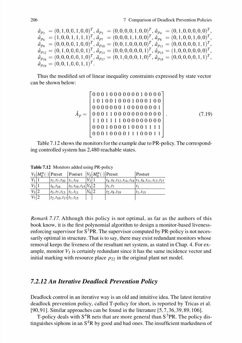
8/4/2019 Li Z., Zhou M. Deadlock Resolution in Automated Manufacturing Systems - A Novel Petri Net Approach
http://slidepdf.com/reader/full/li-z-zhou-m-deadlock-resolution-in-automated-manufacturing-systems-a-novel 219/249
206 7 Comparison of Deadlock Prevention Policies
a p2= (0,1,0,0,1,0,0)T , a p3
= (0,0,0,0,1,0,0)T , a p4= (0,1,0,0,0,0,0)T ,
a p6= (1,0,0,1,1,1,1)T , a p7
= (0,0,0,1,1,0,0)T , a p8= (0,1,0,0,1,0,0)T ,
a p9= (0,0,0,0,1,0,0)T , a p10
= (0,0,1,0,0,0,0)T , a p11= (0,0,0,0,0,1,1)T ,
a p12= (0,1,0,0,0,0,1)T , a p13
= (0,0,0,0,0,0,1)T , a p15= (1,0,0,0,0,0,0)T ,
a p16 = (
0,
0,
0,
0,
0,
1,
0)
T , a p17 = (
0,
1,
0,
0,
0,
1,
0)
T , a p18 = (
0,
0,
0,
0,
0,
1,
1)
T ,
a p19= (0,0,1,0,0,1,1)T .
Thus the modified set of linear inequality constraints expressed by state vector
can be shown below:
ˆ A p =
⎡⎢⎢⎢⎢⎢⎢⎢⎢⎣
0 0 0 1 0 0 0 0 0 0 0 1 0 0 0 0
1 0 1 0 0 1 0 0 0 1 0 0 0 1 0 0
0 0 0 0 0 0 0 1 0 0 0 0 0 0 0 1
0 0 0 1 1 0 0 0 0 0 0 0 0 0 0 0
1 1 0 1 1 1 1 0 0 0 0 0 0 0 0 00 0 0 1 0 0 0 0 1 0 0 0 1 1 1 1
0 0 0 1 0 0 0 0 1 1 1 0 0 0 1 1
⎤⎥⎥⎥⎥⎥⎥⎥⎥⎦. (7.19)
Table 7.12 shows the monitors for the example due to PR-policy. The correspond-
ing controlled system has 2,480 reachable states.
Table 7.12 Monitors added using PR-policy
V S M α 0 (·) Preset Postset V S M α 0 (·) Preset Postset
V 1 1 t 2,t 7,t 20 t 1, t 19 V 2 1 t 4, t 9, t 12,t 14,t 18 t 3,t 8,t 11, t 13, t 17
V 3 1 t 6,t 16 t 5, t 10, t 15 V 4 2 t 3, t 7 t 1V 5 2 t 5,t 7,t 13 t 1, t 11 V 6 2 t 2, t 8, t 19 t 1,t 15
V 7 2 t 2,t 10, t 17 t 1, t 15
Remark 7.17. Although this policy is not optimal, as far as the authors of this
book know, it is the first polynomial algorithm to design a monitor-based liveness-
enforcing supervisor for S3PR. The supervisor computed by PR-policy is not neces-
sarily optimal in structure. That is to say, there may exist redundant monitors whoseremoval keeps the liveness of the resultant net system, as stated in Chap. 4. For ex-
ample, monitor V 3 is certainly redundant since it has the same incidence vector and
initial marking with resource place p22 in the original plant net model.
7.2.12 An Iterative Deadlock Prevention Policy
Deadlock control in an iterative way is an old and intuitive idea. The latest iterative
deadlock prevention policy, called T-policy for short, is reported by Tricas et al.
[90, 91]. Similar approaches can be found in the literature [5,7, 36, 39, 89, 106].
T-policy deals with S4R nets that are more general than S3PR. The policy dis-
tinguishes siphons in an S4R by good and bad ones. The insufficient markedness of

8/4/2019 Li Z., Zhou M. Deadlock Resolution in Automated Manufacturing Systems - A Novel Petri Net Approach
http://slidepdf.com/reader/full/li-z-zhou-m-deadlock-resolution-in-automated-manufacturing-systems-a-novel 220/249
7.2 Applications of Deadlock Prevention Methods to a Case Study 207
the latter is closely related to potential deadlocks. At each iteration, a bad siphon S
is obtained by solving an integer LPP, and then a monitor V S is accordingly added
such that S is max-controlled [4, 8, 107]. The iterative process proceeds until no bad
siphons exist in the resultant net system.
For the example, this policy detects and controls S1, S4, S10, S16, S17, S18, S∗ = p2, p4, p8, p10, p17, p21, p22,V S1,V S16
, and S∗∗ = p2, p3, p8, p9, p12, p13, p16,
p17, V S4, V S17
sequentially. After the eight siphons are controlled, the resultant net
system is live.
Table 7.13 shows the additional monitors due to T-policy for the example. The
process terminates after eight iterations. The resultant controlled system has 14,850
reachable states.
Table 7.13 Monitors added using T-policy
V S M α 0 (·) Preset Postset V S M α 0 (·) Preset PostsetV S1
2 t 10,t 16 t 9, t 15 V S45 t 5,t 10, t 13, t 17 t 3, t 8, t 11, t 15
V S102 t 4,t 13 t 3, t 11 V S16
2 t 9,t 17 t 8, t 16
V S175 t 3,t 8,t 19 t 1, t 17 V S18
2 t 8,t 18 t 7, t 17
V ∗S 5 t 9,t 10,t 16,t 17 2t 8,2t 15 V ∗∗S 3 t 3,t 8,t 17 t 1, t 15
Remark 7.18. In theory, T-policy is still NP-complete since the siphon controlled in
each iteration is found by solving an integer LPP. The number of additional monitors
and the permissive behavior of the resultant supervisor of a plant net model areunknown in advance, which depend on the siphons identified and controlled at each
iteration.
7.2.13 An Optimal Deadlock Prevention Policy Based on Theory of
Regions
The permissive behavior is one of the most important criteria in evaluating the per-formance of a liveness-enforcing or non-blocking supervisor. In terms of the theory
of regions, Uzam [92] develops an optimal liveness-enforcing supervisor synthesis
method, called U1-policy for short. Details of this policy can be found in Chap. 6.
The plant model of the FMS example has 26,750 reachable states, 21,581 of
which are legal, i.e., either good or dangerous states. There are 5,299 elements in
Ω , the set of marking/transition separation instances. This implies that we have to
solve 5,299 LPPs. This policy can in theory lead to an optimal liveness-enforcing
supervisor that results in 21,581 reachable states in the controlled system since such
a supervisor exists from P-policy [77].
Remark 7.19. U1-policy (as well as the one proposed in [34]) can be considered
the only strategy to design an optimal monitor-based supervisor although, due to
the inherent complexity, it is computationally too expensive. In theory, |Ω | is also
8/4/2019 Li Z., Zhou M. Deadlock Resolution in Automated Manufacturing Systems - A Novel Petri Net Approach
http://slidepdf.com/reader/full/li-z-zhou-m-deadlock-resolution-in-automated-manufacturing-systems-a-novel 221/249
208 7 Comparison of Deadlock Prevention Policies
exponential with respect to the size of a plant model. In practice, we have to solve
|Ω | LPPs, which is clearly infeasible for either a sizable net or a small net with a
sizable initial marking.
7.2.14 A Suboptimal Deadlock Prevention Policy
The application of the theory of regions to deadlock prevention is widely extended
after the work in [92] and [34]. The deadlock prevention methods proposed in [93]
and [96] are claimed to require less computational cost to obtain the monitors. They
proceed in an iterative way. At each iteration, a marking called first-met bad mark-
ing (FBM) is identified from the reachability graph of a Petri net model. An FBM is
such a marking in M F that there exists a father node of it in M L. Then, a monitor is
added to prevent the marking from being reached via a well-established invariant-
based control approach [102]. Uzam and Zhou’s method, called U2-policy for short,
in [95] can be considered as an improved version of the deadlock control approaches
in [93] and [96]. The improvement is made since (1) Petri net reduction techniques
are used to simplify a net model so as to find the reachability graph with less compu-
tational overhead; and (2) a simplification for the invariant-based control approach is
proposed. For convenience of discussion, U2-policy is briefly presented as follows:
Input: a plant model G
Output: controlled system G′Step 1. i := 1.
Step 2. Obtain a reduced net model Gi from G by using reduction techniques.
Step 3. Compute the reachability graph RGi for Gi.
Step 4. If Gi is live then G′ := Gi; go to Step 8.
Step 5. Find a first-met bad marking FBM i in Gi.
Step 6. Add monitor V i by defining a P-invariant such that FBM i can never be
reached; denote the resultant net system by G.
Step 7. i := i + 1; go to Step 2.
Step 8. Output controlled system G′.For the example in the case study, the monitors computed by U2-policy are shown
in Table 7.14 after 19 iterations. The corresponding supervisor leads to 21,562
reachable states in the controlled system, and only 0.088% (21,581 − 21,562 =19 out of 21,581) of the maximally permissive behavior is lost.
Remark 7.20. The significance of U2-policy deserves careful considerations from
the standpoint of computational complexity. It is well known that the computation
of a reachability graph is of exponential complexity. As indicated in [34], given the
reachability graph of a plant net model, the computation of a monitor is polynomial.
That is to say, U1-policy needs to compute the reachability graph only once andsolve |Ω | LPP, while, in U2-policy, at each iteration, one has to compute a reacha-
bility graph until all FBM are excluded in the resultant net system. Let k denote the
number of FBM in a net system. We conclude that in theory the number of times of

8/4/2019 Li Z., Zhou M. Deadlock Resolution in Automated Manufacturing Systems - A Novel Petri Net Approach
http://slidepdf.com/reader/full/li-z-zhou-m-deadlock-resolution-in-automated-manufacturing-systems-a-novel 222/249
7.2 Applications of Deadlock Prevention Methods to a Case Study 209
Table 7.14 Monitors added using U2-policy
V S M α 0 (·) Preset Postset V S M α 0 (·) Preset Postset
V 1 2 t 13 t 11 V 2 2 t 4,t 13 t 3, t 12
V 3 2 t 8, t 18 t 7,t 17 V 4 2 t 9,t 17 t 8, t 16
V 5 3 t 8, t 17 t 7,t 16 V 6 2 t 10, t 16 t 9, t 15
V 7 4 t 9, t 17 t 7,t 15 V 8 3 t 10, t 17 t 8, t 15
V 9 4 t 8, t 10,t 17 t 7,t 9,t 15 V 10 5 t 5,t 13, t 17 t 4, t 11, t 15
V 11 5 t 3, t 8, t 19 t 1,t 17 V 12 5 t 5,t 13, t 17 t 3, t 12, t 15
V 13 6 t 5, t 8, t 13,t 17 t 4,t 7,t 11, t 15 V 14 5 t 5,t 10, t 13, t 17 t 4, t 9, t 11, t 15
V 15 6 t 5, t 8, t 13,t 17 t 3,t 7,t 12, t 15 V 16 5 t 5,t 10, t 13, t 17 t 3, t 9, t 12, t 15
V 17 9 t 5, t 8, t 10,t 17,t 19 t 1,t 9,t 15, t 18 V 18 9 t 3,t 5,t 8,t 10, t 18 t 1, t 4, t 9, t 15
V 19 9 t 3, t 5, t 9, t 17,t 19 t 1,t 4,t 15, t 18
computing reachability graphs in U2-policy is equal to k + 1, where k is in theory
exponential with respect to the size of a net model. To summarize, the complexity
of U2-policy is in theory much worse than that of U1-policy. In practice, different
FBM may have common monitor solutions under which they can never be reached.
As a result, the number of times to compute reachability graphs in U2-policy is
(much) smaller than k + 1. In addition, we do notice that some improvements have
been made in U2-policy. However, they cannot significantly reduce its computa-
tional complexity in theory. To summarize, we are led to infer the following points
concerning the two policies:
1. In theory, U1-policy needs to compute the reachability graph only once and tosolve |Ω | LPPs. U2-policy needs to compute the reachability graphs k + 1 times,
where k is the number of FBM in M F . |Ω | and k have the same order of magni-
tude, which, in theory, are exponential with respect to the size of a net.
2. In practice, both of them first compute the reachability graph of a plant. Then,
U1-policy has to solve |Ω | LPPs in order to decide whether different mark-
ing/transition instances have the common monitor solutions. While, the number
of times to compute reachability graphs in U2-policy may be small due to the
fact that different FBMs often have common monitor solutions. The practical ex-
amples even suggest that it is exponentially smaller than k as each FBM oftenrepresents the first one that leads to a large portion of bad markings. Its control
means this portion’s control.
In theory U1-policy as well as the one proposed in [34], in which the reachability
graph of a plant net model needs to be computed only once, remains to be an elegant
strategy in designing a liveness-enforcing supervisor with maximally permissive be-
havior (provided that such a supervisor exists). However, in practice, the superiority
of the one over the other remains open. Compared with U1-policy, U2-policy seems
promising when we deal with a net in which
|Ω
|is large but the state space is small.
However, it is taken for granted that a small state space of a plant net model usuallyhas a small |Ω |. In this scenario, intuitively, U2-policy is computationally better
than U1-policy. More work is needed to compare them by the study of examples
whose state spaces range from being small to large.

8/4/2019 Li Z., Zhou M. Deadlock Resolution in Automated Manufacturing Systems - A Novel Petri Net Approach
http://slidepdf.com/reader/full/li-z-zhou-m-deadlock-resolution-in-automated-manufacturing-systems-a-novel 223/249
210 7 Comparison of Deadlock Prevention Policies
7.2.15 An Optimal Policy Based on Complete Siphon Enumeration
For S3PR nets, the deadlock prevention policy, called X-policy for short, proposed
by Xing and Hu in [101] aims, by structural analysis, to develop a liveness-enforcing
supervisor with maximally permissive behavior and a minimized number of addi-tional monitors.
The concepts of perfect resource transition circuits (PRT-circuits) and their satu-
rated states are proposed. A saturated PRT-circuit implies the existence of circular
wait that is tied to deadlock states. The liveness of an S3PR net is characterized by
the fact that no PRT-circuit can reach a saturated state at any reachable marking of
the system.
Starting from PRT-circuits, elementary maximal PRT-circuits and center re-
sources are accordingly defined. A center resource has a capacity of one and is
contained in the resource sets of at least two elementary maximal PRT-circuits. Thefollowing facts are claimed [101]:
1. For an S3PR without center resources, an optimal liveness-enforcing supervisor
can be obtained by computing a set of monitors.
2. An S3PR net model with center resources can be reduced to a simple one SPN(r)
by removing center resources according to a set of rules. An optimal liveness-
enforcing supervisor PC(r) can be found for SPN(r). The composition of PC(r)
and SPN(r) can derive a supervisory policy ρ under which the system is live.
3. Each elementary maximal PRT-circuit can be used to derive a strict minimal
siphon and vice versa.
4. X-policy needs the complete siphon enumeration and hence is of exponential
complexity.
For an elementary maximal PRT-circuit θ with its resource place set R[θ ], a
monitor pθ is added by the siphon control approach of AE-policy with M α 0 ( pθ ) = M 0( R[θ ]) − 1.
The example has a center resource R2( p21). The reduced Petri net model resulting
from removing p21 is shown in Fig.7.1. Table 7.15 shows the monitors of PC(r) for
the reduced net model SPN(r) of the example. A supervisory policy derived fromthe synchronous synthesis of PC(r) and SPN(r) can lead to the controlled system
that has 16,276 reachable states.
Table 7.15 Monitors added using X-policy in PC(r)
V S M α 0 (·) Preset Postset V S M α 0 (·) Preset Postset
V 1 2 t 10, t 16 t 8,9, t 15 V 2 3 t 8,9, t 17,18 t 7, t 16
V 3 4 t 10, t 17,18 t 7, t 15 V 4 9 t 5, t 10, t 19 t 1, t 15
Remark 7.21. The rationality of X-policy is worthy of being further investigated
when a plant net model contains center resources although it is theoretically correct
that the removal of the center resources can lead to an optimal supervisor.

8/4/2019 Li Z., Zhou M. Deadlock Resolution in Automated Manufacturing Systems - A Novel Petri Net Approach
http://slidepdf.com/reader/full/li-z-zhou-m-deadlock-resolution-in-automated-manufacturing-systems-a-novel 224/249
7.3 Analysis of Deadlock Prevention Methods 211
p 1 p 3
p 5
p 6
p 7
p 9
p 1 0
p 1 1
p 1 3
p 1 4
p 1 5
p 1 6
p 1 8
p 1 9
p 2 0
p 2 2
p 2 3
p 2 4
p 2 5
p 2 6
t 1
t 2
t 3 , 4
t 5
t 6
t 7
t 8 , 9
t 1 0
t 1 1 , 1 2
t 1 3 , 1 4
t 1 5
t 1 6
t 1 7 , 1 8
t 1 9
t 2 0
M 1
M 2
M 3
M 4
R 1
R 3
I 1 / O 1 I 2 / O 2
I 3 / O 3
7
1 1
3
Fig. 7.1 The reduced Petri net model SPN(r) of the example
Remark 7.22. While X-policy guarantees the optimality of deadlock control for
S3PR without center resources, some S3PR with center resources may also be opti-
mally controlled. For example, the net depicted in Fig. 6.9 has center resources but
an optimal liveness-enforcing supervisor can be found by computing four monitors
for the strict minimal siphons.
7.3 Analysis of Deadlock Prevention Methods
Table 7.16 summarizes the performance of the supervisors resulting from the poli-
cies recounted in the last section. The first column lists the policies and the second
denotes the number of reachable states of the corresponding supervisor. The third
and fourth columns show the number of the additional monitors and arcs, respec-
tively. The fifth (sixth) indicates whether the complete siphon (state) enumeration is
necessary in a policy (“√
” means “yes” and “×” means “no”). The seventh column
exhibits the computational complexity. We do not present here the specific computa-
tion time of these policies for this example since the necessary computation requiredby each of them can be finished within a few seconds or, at most, a few minutes (ex-
cept for U1-policy) in a personal computer. Note that for the example in this case
study the monitors and arcs due to U1-policy can be computed with commercial

8/4/2019 Li Z., Zhou M. Deadlock Resolution in Automated Manufacturing Systems - A Novel Petri Net Approach
http://slidepdf.com/reader/full/li-z-zhou-m-deadlock-resolution-in-automated-manufacturing-systems-a-novel 225/249
212 7 Comparison of Deadlock Prevention Policies
software packages. No results of this case example are found in the literature by
using U1-policy.
Table 7.16 Performance analysis and comparison
Policy
in the
literature
No.
reach.
states
No.
add.
monitors
No.
add.
arcs
Complete
siphon
enumeration
Complete
reach.
graph
Computational
Complexity
AE-policy × 18 104√ × exponential
B1-policy × 18 104√ × exponential
B2-policy 166 0 0√ × exponential
P-policy 21,581 13 82√ × exponential
E-policy 6,287 18 106√ × exponential
H1-policy 12,656 16 88 × × NP-hard
H2-policy 16,425 7 34√ × exponential
L1-policy 6,287 6 32 √ × exponentialL2-policy 6,331 5 27 × × NP-hard
L3-policy 15,999 6 29 × × NP-hard
PR-policy 2,480 7 38 × × polynomial
T-policy 14,850 8 40 × × NP-hard
U1-policy 21,581 × × × √exponential
U2-policy 21,562 19 112 × √exponential
X-policy 15,098 4 17√ × exponential
The performance analysis of the policies is carried out by considering the follow-ing three criteria: behavior permissiveness, computational complexity, and structural
complexity.
7.3.1 Reachability-Graph-Based Policies
U1- and U2-policies fall under this class of deadlock prevention methods. The su-
pervisors derived from them can usually have maximally permissive behavior if
such supervisors exist. Since the computation of the reachability graph for a plant
net model is necessary, these policies are of exponential complexity. The number
of additional monitors is, in theory, equal to that of marking/transition separation
instances or that of FBMs. Although, as indicated by the case study, different mark-
ing/transition separation instances or FBMs can have common monitor solutions, as
far as the authors know, there is no formal proof indicating that in practice the num-
ber of monitors is polynomial with respect to the size of the plant. These policies
cannot deal with a large-sized net with a large initial marking due to the state explo-
sion problem [14, 17]. By INA [86], we have tried to find the reachability graph for
an S3PR net model with 68 places and 54 transitions. The computation was carriedout on a Toshiba notebook with 1.7 GHz processor speed and 512 M of memory
under the Windows XP operating system. After having generated 1,764,263 states
in more than six days, the computation aborted due to memory overflow.

8/4/2019 Li Z., Zhou M. Deadlock Resolution in Automated Manufacturing Systems - A Novel Petri Net Approach
http://slidepdf.com/reader/full/li-z-zhou-m-deadlock-resolution-in-automated-manufacturing-systems-a-novel 226/249
7.3 Analysis of Deadlock Prevention Methods 213
It is worthy of note that symbolic techniques based on binary decision dia-
grams [9, 10] have emerged as an efficient strategy for the reachability analysis and
computation of Petri nets [71,74,75]. These methods are expected to be used in the
resolution of deadlocks in FMSs in the future.
7.3.2 Complete-Siphon-Enumeration-Based Policies
As a structural object, siphons are extensively used in the analysis and control of
deadlocks in resource allocation systems [15, 42, 79–82], leading to a large number
of siphon-based deadlock control strategies [59,64–66,88]. In this chapter, AE-, B1-
, B2-, P-, E-, H2-, L1-, and X-policies fall under the class of deadlock prevention
methods that need the complete siphon enumeration of a plant net model.
In general, a siphon-based deadlock prevention policy cannot lead to a maxi-
mally permissive liveness-enforcing supervisor except for the nets with particular
structures or initial markings. Siphons in a Petri net are a purely structural object
whose computation is independent of markings. However, it is well known that their
number grows fast and in the worst case grows exponentially with respect to the size
of a net [18,46]. It seems that siphon-based methods can deal well with the deadlock
problems in a small net structure with any initial marking. In this sense, a siphon-
based method, compared with the ones based on reachability graphs, behaves much
better from the standpoint of computational complexity.
For the example investigated in this chapter, it is easy to see that the structure of
a supervisor can be simplified if the elementary siphons are taken into account when
one designs a deadlock prevention policy. An elegant result concerning elementary
siphon theory is that a dependent siphon can be controlled by properly supervising
its elementary siphons. This implies that, in theory, monitors can be added for el-
ementary siphons only. Since the number of the elementary siphons is bounded by
the smaller of place and transition counts, it can be concluded that an elementary
siphon-based deadlock prevention policy can usually lead to a structurally simple
liveness-enforcing supervisor.
7.3.3 Partial-Siphon-Enumeration-Based Policies
In theory, behavior permissiveness of a supervisor does not depend on whether or
not a policy needs complete siphon enumeration. From the case study, a deadlock
prevention policy that needs partial siphon enumeration may lead to a supervisor
with more permissive behavior and simplified net structure. H1-, L2-, L3-, PR-,
and T-policies belong to this class of methods. From the standpoint of performanceof the supervisors, these policies make a favorable balance between computational
complexity and behavior permissiveness. For example, as shown in [61], it takes
more than 6 hours to compute all 169 strict minimal siphons in an S 3PR with 68

8/4/2019 Li Z., Zhou M. Deadlock Resolution in Automated Manufacturing Systems - A Novel Petri Net Approach
http://slidepdf.com/reader/full/li-z-zhou-m-deadlock-resolution-in-automated-manufacturing-systems-a-novel 227/249
214 7 Comparison of Deadlock Prevention Policies
places and 54 transitions by using INA. However, L3-policy just needs to compute
24 strict minimal siphons and to control 13 of them, taking 178 seconds only, where
Lindo [68] is used to solve the MIP problems. Except the PR-policy, which is of
polynomial complexity, most deadlock prevention policies requiring no complete
siphon enumeration need to solve MIP problems, which is NP-hard. However, theexperimental study of many cases shows that PR-policy is over-conservative.
7.3.4 Exponential Complexity and NP-Hardness
Except PR-policy [73], which is of polynomial-time, other existing deadlock pre-
vention policies need either the (partial or complete) siphon enumeration or reach-
ability graph. A policy is classified into the class with exponential complexity if it
needs the complete siphon enumeration or reachability graph. As is well-known, the
number of siphons in a Petri net grows in the worst case exponentially with respect
to its size and the size of reachability graph grows exponentially with the size of the
net as well as initial markings. A policy is of NP-hard complexity if it involves the
solution of an MIP problem.
Recognizing the inefficiency and intractability of computing the complete siphon
enumeration and reachability graph for a Petri net, the MIP-based method [13] is a
fast deadlock detection approach for structurally bounded nets whose deadlocks are
tied to unmarked siphons. Although an MIP problem is NP-hard and is difficult to
solve [33], the case study conducted by Chu and Xie [13] shows that its compu-
tational efficiency is relatively insensitive to the initial marking and it seems to be
much more efficient than the classical complete state or siphon enumeration meth-
ods.
H1-, L2-, L3-, and T-policies use the MIP-based deadlock detection method to
avoid the complete siphon enumeration. In each of these policies, the number of
times of solving MIP problems is in theory exponential with respect to the size of a
net [88]. In practice, the number of the iteration steps is in general much smaller than
that of deadlock states since different deadlock states may share a common monitor
solution, which leads to the relatively high efficiency of these deadlock preventionpolicies.
Remark 7.23. When behavior permissiveness is not a major concern, PR-policy
should be the best choice for industrial-size automated systems as it is the only
deadlock prevention approach in the literature with polynomial complexity. If the
off-line computational cost is not a problem and the computation is feasible, U1- or
U2-policies should be the first choice of industrial engineers. The deadlock preven-
tion policies that use partial siphon enumeration achieve a good balance between
the behavior permissiveness and computational complexity [84].
Remark 7.24. A natural extension to the current work is to improve the computa-
tional efficiency of deadlock prevention methods that are based on the theory of

8/4/2019 Li Z., Zhou M. Deadlock Resolution in Automated Manufacturing Systems - A Novel Petri Net Approach
http://slidepdf.com/reader/full/li-z-zhou-m-deadlock-resolution-in-automated-manufacturing-systems-a-novel 228/249
7.4 Bibliographical Remarks 215
regions [83]. Future work can also focus on the development of elementary siphon-
based deadlock control methods. As a conjecture, if a polynomial algorithm is de-
veloped to find a set of elementary siphons for a particular class of Petri nets [97], it
is possible that we can develop a number of polynomial deadlock control methods
for the net class, which are supposed to be more permissive than PR-policy.
7.4 Bibliographical Remarks
Most of the material in this chapter is from the recent work [67]. It is hard to com-
pare, from a theoretical point of view or by a formal proof, the behavior permis-
siveness of two deadlock prevention strategies if both of them are not optimal. As
a result, experimental study seems to be an effective way to find an answer to this
problem. It is a time-consuming and tedious task since we need a fair number of
Petri nets generated randomly.
The paper by Fanti and Zhou [29] compares the deadlock control approaches
for automated manufacturing systems under different formalisms such as Petri nets,
graph theory [12, 22–30, 98, 99], automata [69], and the combination of these for-
malisms [48–56, 70,76, 94]. Not much work except [6, 21,31, 35,37, 60,72] is found
in the literature to compare different deadlock control strategies for FMS.
Problems
7.1. Design liveness-enforcing supervisors for S3PR shown in Fig. 5.3 by the dead-
lock prevention policies in Sect. 7.2. Compare the resultant supervisors in terms of
structural complexity, computational cost, and permissive behavior. Note that an op-
timal liveness-enforcing supervisor of the Petri net model should lead to a controlled
system that has 60 reachable states.
7.2. Design liveness-enforcing supervisors for S3
PR shown in Fig. 5.16 by the dead-lock prevention policies in Sect. 7.2. Compare the resultant supervisors in terms of
structural complexity, computational cost, and permissive behavior. Note that an
optimal controlled system should have 205 reachable states.
7.3. Design liveness-enforcing supervisors for S3PR shown in Fig. 6.7 by the dead-
lock prevention policies in Sect. 7.2. Compare the resultant supervisors in terms of
structural complexity, computational cost, and permissive behavior. Note that an op-
timal controlled system of the Petri net model should have 48 reachable states. A fact
can be easily observed that some of the policies lead to optimal liveness-enforcing
supervisors.
7.4. Design a liveness-enforcing supervisor for S3PR shown in Fig. 6.7 by P-policy
proposed in [77].
8/4/2019 Li Z., Zhou M. Deadlock Resolution in Automated Manufacturing Systems - A Novel Petri Net Approach
http://slidepdf.com/reader/full/li-z-zhou-m-deadlock-resolution-in-automated-manufacturing-systems-a-novel 229/249
216 7 Comparison of Deadlock Prevention Policies
7.5. As seen in Subsect. 7.2.5, E-policy adds 18 monitors for the FMS example in
this chapter. Find the implicit places in the controlled system.
References
1. Abdallah, I.B., ElMaraghy, H.A. (1998) Deadlock prevention and avoidance in FMS: A Petri
net based approach. International Journal of Advanced Manufacturing Technology, vol.14,
no.10, pp.704–715.2. Barkaoui, K., Abdallah, I.B. (1995) A deadlock prevention method for a class of FMS. In
Proc. IEEE Int. Conf. on Systems, Man, and Cybernetics, pp.4119–4124.3. Barkaoui, K., Abdallah, I.B. (1995) Deadlock avoidance in FMS based on structural theory
of Petri nets. In Proc. INRIA/IEEE Symposium on Emerging Technologies and Factory Au-
tomation, pp.499–510.
4. Barkaoui, K., Pradat-Peyre, J.F. (1996) On liveness and controlled siphons in Petri nets. InProc. 17th Int. Conf. on Applications and Theory of Petri Nets Lecture Notes in Computer
Science, vol.1091, pp.57–72.5. Barkaoui, K., Chaoui, A., Zouari, B. (1997) Supervisory control of discrete event systems
based on structure theory of Petri nets. In Proc. IEEE Int. Conf. on Systems, Man, and Cyber-
netics, pp.3750–3755.6. Barkaoui, K., Chaoui, A., Benamara, R. (1997) The performance of alternative strategies for
dealing with deadlocks in FMS. In Proc. 6th Int. Conf. on Emerging Technologies and Factory
Automation, pp.281–286.7. Barkaoui, K., Petrucci, L. (1998) Structural analysis of workflow nets with shared resources.
In Proc. Workshop on Workflow Management: Net-based Concepts, Models, Techniques and
Tools, pp.82–95.8. Barkaoui, K., Couvreur, J.M., Klai, K. (2005) On the equivalence between liveness and
deadlock-freeness in Petri nets. In Proc. 26th Int. Conf. on Applications and Theory of Petri
Nets and Other Models of Concurrency, Lecture Notes in Computer Science, vol.3536, pp.90–
107.9. Bryant, R.E. (1986) Graph-based algorithms for Boolean function manipulation. IEEE Trans-
actions on Computers, vol.35, no.8, pp.677–691.10. Bryant, R.E. (1992) Symbolic boolean manipulation with ordered binary-decision diagrams.
ACM Computing Surveys, vol.24, no.3, pp.293–318.11. Chao, D.Y. (2006) Maximal class of weakly live nets without emptiable siphons. IEEE Trans-
actions on Systems, Man, and Cybernetics, Part B, vol.36, no.6, pp.1332–1341.12. Cho, H., Kumaran, T.K., Wysk, R.A. (1995) Graph-theoretic deadlock detection and reso-
lution for flexible manufacturing systems. IEEE Transactions on Robotics and Automation,
vol.11, no.3, pp.413–421.13. Chu, F., Xie, X.L. (1997) Deadlock analysis of Petri nets using siphons and mathematical
programming. IEEE Transactions on Robotics and Automation, vol.13, no.6, pp.793–804.14. Ciardo, G. (2004) Reachability set generation for Petri nets: can brute force be smart? In Proc.
25th Int. Conf. on Applications and Theory of Petri Nets, Lecture Notes in Computer Science,
vol.3099, pp.17–34.15. Colom, J.M. (2003) The resource allocation problem in flexible manufacturing systems. In
Proc. Int. Conf. on Applications and Theory of Petri Nets, W. van der Aalst and E. Best
(Eds.), Lecture Notes in Computer Science, vol. 2679, pp.23–35.16. Cordone, R., Ferrarini, L., Piroddi, L. (2005) Enumeration algorithms for minimal siphons in
Petri nets based on place constraints. IEEE Transactions on Systems, Man and Cybernetics,Part A, vol.35, no.6, pp.844–854.
17. Esparza, J. (1998) Decidability and complexity of Petri net problems – an introduction. In
Lectures on Petri Nets I: Basic Models, Lecture Notes in Computer Science, vol.1491, G.
Rozenberg and W. Reisig (Eds.), pp.374–428.
8/4/2019 Li Z., Zhou M. Deadlock Resolution in Automated Manufacturing Systems - A Novel Petri Net Approach
http://slidepdf.com/reader/full/li-z-zhou-m-deadlock-resolution-in-automated-manufacturing-systems-a-novel 230/249
References 217
18. Ezpeleta, J., Couvreur, J.M., Silva, M. (1993) A new technique for finding a generating family
of siphons, traps, and st-components: Application to colored Petri nets. In Advances in Petri
Nets, Lecture Notes in Computer Science, vol.674, G. Rozenberg (Eds.), pp.126–147.
19. Ezpeleta, J, Colom, J.M., Martinez, J. (1995) A Petri net based deadlock prevention policy
for flexible manufacturing systems. IEEE Transactions on Robotics and Automation, vol.11,
no.2, pp.173–184.20. Ezpeleta, J., Garcıa-Valles, F., Colom, J.M. (1998) A class of well structured Petri nets for
flexible manufacturing systems. In Proc. 19th Int. Conf. on Applications and Theory of Petri
Nets, Lecture Notes in Computer Science, vol.1420, J. Desel and M. Silva (Eds.), pp.64–83.
21. Fanti, M.P., Maione, B., Mascolo, S., Turchiano, B. (1996) Performance of deadlock avoid-
ance algorithms in flexible manufacturing systems. Journal of Manufacturing Systems, vol.15,
no.3, pp.164–178.
22. Fanti, M.P., Maione, B., Mascolo, S., Turchiano, B. (1997) Event-based feedback control
for deadlock avoidance in flexible production systems. IEEE Transactions on Robotics and
Automation, vol.13, no.3, pp.347–363.
23. Fanti, M.P., Maione, B., Turchiano, B. (2000) Comparing digraph and Petri net approaches to
deadlock avoidance in FMS. IEEE Transactions on Systems, Man, and Cybernetics, Part B,vol.30, no.5, pp.783–798.
24. Fanti, M.P., Maione, B., Turchiano, B. (2001) Distributed event-control for deadlock avoid-
ance in automated manufacturing systems. International Journal of Production Research,
vol.39, no.9, pp.1993–2021.
25. Fanti, M.P., Turchiano, B. (2001) Deadlock avoidance in automated guided vehicle systems.
In Proc. IEEE/ASME International Conference on Advanced Intelligent Mechatronics, vol.2,
pp.1017–1022.
26. Fanti, M.P. (2002) Event-based controller to avoid deadlock and collisions in zone-control
AGVS. International Journal of Production Research, vol.40, no.6, pp.1453–1478.
27. Fanti, M.P., Maione, B., Turchiano, B. (2002) Design of supervisors to avoid deadlock in
flexible assembly systems. International Journal of Flexible Manufacturing Systems, vol.14,no.2, pp.157–175.
28. Fanti, M.P. (2004) Deadlock resolution strategy for automated manufacturing systems includ-
ing conjunctive resource service. IEEE Transactions on Systems, Man, and Cybernetics, Part
A, vol.34, no.1, pp.80–92.
29. Fanti, M.P., Zhou, M.C. (2004) Deadlock control methods in automated manufacturing sys-
tems. IEEE Transactions on Systems, Man, and Cybernetics, Part A, vol.34, no.1, pp.5–22.
30. Fanti, M.P., Zhou, M.C. (2005) Deadlock control methods in automated manufacturing sys-
tems. In Deadlock Resolution in Computer-Integrated Systems, New York: Marcel Dekker,
pp.1–22.
31. Ferrarini, L., Piroddi, L. (2005) The effect of modeling and control techniques on the man-
agement of deadlocks in FMS. In Deadlock Resolution in Computer-Integrated System, M.C. Zhou and M. P. Fanti, (Eds)., New York: Marcel Dekker, pp.407–444.
32. Garcıa-Valles, F., Colom, J.M. (1999) Implicit places in net systems. In Proc. 8th Int. Work-
shop on Petri Nets and Performance Models, pp.104–113.
33. Garey, M.R., Johnson, D.S. (1979) Computers and Intractability: A Guide to the Theory of
NP-Completeness. New York: W. H. Freeman.
34. Ghaffari, A., Rezg, N., Xie, X.L. (2003) Design of a live and maximally permissive Petri
net controller using the theory of regions. IEEE Transactions on Robotics and Automation,
vol.19, no.1, pp.137–142.
35. Hosack, B., Mahmoodi, F., Mosier, C.T. (2003) A comparison of deadlock avoidance policies
in flexible manufacturing systems. International Journal of Production Research, vol.41, no.
13, pp.2991–3006.36. Huang, Y.S., Jeng, M.D., Xie, X.L., Chung, S. L. (2001) Deadlock prevention policy based on
Petri nets and siphons. International Journal of Production Research, vol.39, no.2, pp.283–
305.

8/4/2019 Li Z., Zhou M. Deadlock Resolution in Automated Manufacturing Systems - A Novel Petri Net Approach
http://slidepdf.com/reader/full/li-z-zhou-m-deadlock-resolution-in-automated-manufacturing-systems-a-novel 231/249
218 7 Comparison of Deadlock Prevention Policies
37. Huang, Y.S., Lin, J.H., Hsu, C.N., (2004) Comparison of deadlock prevention policies in
FMS based on Petri nets siphons. In Proc. IEEE Int. Conf. on Systems, Man, and Cybernetics,
pp.4867–4872.
38. Huang, Y.S. (2007) Design of deadlock prevention supervisors for FMS using Petri nets.
International Journal of Advanced Manufacturing Technology, vol.35, no.3–4, pp.349–362.
39. Iordache, M.V., Moody, J.O., Antsaklis, P.J. (2002) Synthesis of deadlock prevention supervi-sors using Petri nets. IEEE Transactions on Robotics and Automation, vol.18, no.1, pp.59–68.
40. Jeng, M.D., DiCesare, F. (1995) Synthesis using resource control nets for modeling shared-
resource systems. IEEE Transactions on Robotics and Automation, vol.11, no.3, pp.317–327.
41. Jeng, M.D. (1997) A Petri net synthesis theory for modeling flexible manufacturing systems.
IEEE Transactions on Systems, Man and Cybernetics, Part B, vol.27, no.2, pp.169–183.
42. Jeng, M.D., Peng, M.Y., Huang, Y.S. (1999) An algorithm for calculating minimal siphons
and traps in Petri nets. International Journal of Intelligent Control and Systems, vol.3, no.3,
pp.263–275.
43. Jeng, M.D., Xie, X.L. (1999) Analysis of modularly composed nets by siphons. IEEE Trans-
actions on Systems, Man, and Cybernetics, Part A, vol.29, no.4, pp.399–406.
44. Jeng, M.D., Xie, X.L., Peng, M.Y. (2002) Process nets with resources for manufacturingmodeling and their analysis. IEEE Transactions on Robotics and Automation, vol.18, no.6,
pp.875–889.
45. Jeng, M.D., Xie, X.L., Chung, S.L. (2004) ERCN* merged nets for modeling degraded be-
havior and parallel processes in semiconductor manufacturing systems. IEEE Transactions
on Systems, Man, and Cybernetics, Part A, vol.34, no.1, pp.102–112.
46. Lautenbach, K. (1987) Linear algebraic calculation of deadlocks and traps. In Concurrency
and Nets, K. Voss, H. J. Genrich and G. Rozenberg (Eds.), pp.315–336.
47. Lautenbach, K., Ridder, H. (1996) The linear algebra of deadlock avoidance – a Petri net
approach. No.25-1996, Technical Report, Institute of Software Technology, University of
Koblenz-Landau, Koblenz, Germany.
48. Lawley, M.A., Reveliotis, S.A., Ferreira, P.M. (1997) Design guidelines for deadlock-handling strategies in flexible manufacturing systems. International Journal of Flexible Man-
ufacturing Systems, vol.9, no.1, pp.5–30.
49. Lawley, M.A., Reveliotis, S.A., Ferreira, P.M. (1998) Flexible manufacturing system struc-
tural control and the neighborhood policy, part 2. Generalization, optimization, and efficiency.
IIE Transactions, vol.29, no.10, pp.889–899.
50. Lawley, M.A., Reveliotis, S.A., Ferreira, P.M. (1998) A correct and scalable deadlock avoid-
ance policy for flexible manufacturing systems. IEEE Transactions on Robotics and Automa-
tion, vol.14, no.5, pp.796–809.
51. Lawley, M.A., Reveliotis, S.A., Ferreira, P.M. (1998) Flexible manufacturing system struc-
tural control and the neighborhood policy, part 1. Correctness and Scalability. IIE Transac-
tions, vol.29, no.10, pp.877–887.52. Lawley, M.A., Reveliotis, S.A., Ferreira, P.M. (1998) The application and evaluation of
banker’s algorithm for deadlock-free buffer space allocation in flexible manufacturing sys-
tems. International Journal of Flexible Manufacturing Systems, vol.10, no.1, pp.73–100.
53. Lawley, M.A. (1999) Deadlock avoidance for production systems with flexible routing. IEEE
Transactions on Robotics and Automation, vol.15, no.3, pp.497–509.
54. Lawley, M.A. (2000) Integrating flexible routing and algebraic deadlock avoidance policies
in automated manufacturing systems. International Journal of Production Research, vol.38,
no.13, pp.2931–2950.
55. Lawley, M.A., Reveliotis, S.A. (2001) Deadlock avoidance for sequential resource alloca-
tion systems: Hard and easy cases. International Journal of Flexible Manufacturing Systems,
vol.13, no.4, pp.385–404.56. Lawley, M.A., Sulistyono, W. (2002) Robust supervisory control policies for manufacturing
systems with unreliable resources. IEEE Transactions on Robotics and Automation, vol.18,
no.3, pp.346–359.

8/4/2019 Li Z., Zhou M. Deadlock Resolution in Automated Manufacturing Systems - A Novel Petri Net Approach
http://slidepdf.com/reader/full/li-z-zhou-m-deadlock-resolution-in-automated-manufacturing-systems-a-novel 232/249
References 219
57. Li, Z.W., Zhou, M.C. (2004) Elementary siphons of Petri nets and their application to dead-
lock prevention in flexible manufacturing systems. IEEE Transactions on Systems, Man, and
Cybernetics, Part A, vol.34, no.1, pp.38–51.
58. Li, Z.W., Uzam, M., Zhou, M.C. (2004) Comments on “Deadlock prevention policy based
on Petri nets and siphons”. International Journal of Production Research, vol.42, no.24,
pp.5253–5254.59. Li, Z.W., Zhou, M.C. (2005) Elementary siphon of Petri nets for effective deadlock control in
flexible manufacturing systems. In Deadlock Resolution in Computer-Integrated Systems, M.
C. Zhou and M. P. Fanti (Eds.), New York: Marcel Dekker, pp. 309–348.
60. Li, Z.W., Zhou, M.C. (2005) Comparison of two deadlock prevention methods for different-
size flexible manufacturing systems. International Journal of Intelligent Control and Systems,
vol.10, no.3, pp.235–243.
61. Li, Z.W., Zhou, M.C. (2006) Two-stage method for synthesizing liveness-enforcing super-
visors for flexible manufacturing systems using Petri nets. IEEE Transactions on Industrial
Informatics, vol.2, no.4, pp.313–325.
62. Li, Z.W., Zhou, M.C. (2006) Clarifications on the definitions of elementary siphons of Petri
nets. IEEE Transactions on Systems, Man, and Cybernetics, Part A, vol.36, no.6, pp.1227–1229.63. Li, Z.W., Hu, H.S., Wang, A.R. (2007) Design of liveness-enforcing supervisors for flexible
manufacturing systems using Petri nets. IEEE Transactions on Systems, Man, and Cybernet-
ics, Part C , vol.37, no.4, pp.517–526.
64. Li, Z.W., Zhou, M.C., Uzam, M. (2007) Deadlock control policy for a class of Petri nets
without complete siphon enumeration. IET Control Theory and Applications, vol.1, no.6,
pp.1594–1605.
65. Li, Z.W., Zhang, J, Zhao, M. (2007) Liveness-enforcing supervisor design for a class of gen-
eralized Petri net models of flexible manufacturing systems. IET Control Theory and Appli-
cations, vol.1, no.4, pp.955–967.
66. Li, Z.W., Sheptalni, M. (2009) A smart deadlock prevention policy for flexible manufacturing
systems using Petri nets. To appear in IET Control Theory and Applications.
67. Li, Z.W., Zhou, M.C. (2008) A survey and comparison of Petri net-based deadlock preven-
tion policies for flexible manufacturing systems. IEEE Transactions on Systems, Man, and
Cybernetics, Part C , vol.38, no.2, pp.172–188.68. Lindo, Premier Optimization Modeling Tools, http://www.lindo.com/.
69. Ma, C., Wonham, W.M. (2005) Nonblocking Supervisory Control of State Tree Structures.
Berlin: Springer.
70. Maione, G., DiCesare F. (2005) Hybrid Petri net and digraph approach for deadlock pre-
vention in automated manufacturing systems. International Journal of Production Research,
vol.43, no.24, pp.5131–5159.71. Miner, A.S., Ciardo, G. (1999) Efficient reachability set generation and storage using deci-
sion diagrams. In Proc. Int. Conf. on Application and Theory of Petri Nets, Lecture Notes in
Computer Science, vol.1639, pp.6–25.
72. Mohan, S., Yalcin, A., Khator, S. (2004) Controller design and performance evaluation
for deadlock avoidance in automated flexible manufacturing cells. Robotics and Computer-
Integrated Manufacturingvol.20, no.6, pp.541–551.
73. Park, J., Reveliotis, S.A. (2001) Deadlock avoidance in sequential resource allocation systems
with multiple resource acquisitions and flexible routings. IEEE Transactions on Automatic
Control, vol.46, no.10, pp.1572–1583.
74. Pastor, E., Cortadella, J., Pena, M.A. (1999) Structural methods to improve the symbolic
analysis of Petri nets. In Proc. Int. Conf. on Application and Theory of Petri Nets, Lecture
Notes in Computer Science, vol.1639, pp.26–45.
75. Pastor, E., Cortadella, J., Roig, O. (2001) Symbolic analysis of bounded Petri nets. IEEE Transactions on Computers, vol.50, no.5, pp.432–448.
76. Pinzon, L.E., Hanisch, H.M., Jafari, M.A., Boucher, T. (1999) A comparative study of syn-
thesis methods for discrete event controllers. Formal Methods in System Design, vol.15, no.2,
pp.123–167.

8/4/2019 Li Z., Zhou M. Deadlock Resolution in Automated Manufacturing Systems - A Novel Petri Net Approach
http://slidepdf.com/reader/full/li-z-zhou-m-deadlock-resolution-in-automated-manufacturing-systems-a-novel 233/249
220 7 Comparison of Deadlock Prevention Policies
77. Piroddi, L., Cordone, R., Fumagalli, I. (2008) Selective siphon control for deadlock preven-
tion in Petri nets. IEEE Transactions on Systems, Man, and Cybernetics, Part A, vol. 38, no.
6, pp.1337–1348.
78. Recalde, L., Teruel, E., Silva, M., (1997) Improving the decision power of rank theorems. In
Proc. IEEE Int. Conf. on Systems, Man, and Cybernetics, pp.3768–3773.
79. Reveliotis, S.A. (2002) Liveness enforcing supervision for sequential resource allocation sys-tems: state of the art and open issues. In Synthesis and Control of Discrete Event Systems, B.
Caillaud, X. L. Xie, P. Darondeau, and L. Lavagno (Eds.), Boston, MA: Kluwer, pp.203–212.
80. Reveliotis, S.A. (2003) On the siphon-based characterization of liveness in sequential re-
source allocation systems. In Proc. Int. Conf. on Applications and Theory of Petri Nets,
Lecture Notes in Computer Science, vol.2679, W. M. P. van der Aalst and E. Best (Eds.),
pp.241–255.
81. Reveliotis, S.A. (2005) On the siphon-based characterization of liveness and liveness-
enforcing supervision for sequential resource allocation systems. In Deadlock Resolution in
Computer-Integrated Systems, pp.283–307, New York: Marcel Dekker.
82. Reveliotis, S.A. (2005) Real-time Management of Resource Allocation Systems: A Discrete
Event Systems Approach, New York: Springer.83. Reveliotis, S.A., Choi, J.Y. (2006) Designing reversibility-enforcing supervisors of polyno-
mial complexity for bounded Petri nets through the theory of regions. In Proc. 27th Int. Conf.
on Applications and Theory of Petri Nets and Other Models of Concurrency, Lecture Notes
in Computer Science, vol.4024, S. Donatelli and P. S. Thiagarajan (Eds.), pp.322–341.
84. Reveliotis, S.A., Roszkowska, E., Choi, J.Y. (2007) Generalized algebraic deadlock avoidance
policies for sequential resource allocation systems. IEEE Transactions on Automatic Control,
vol.52, no.12, pp.2345–2350.
85. Silva, M., Teruel, E., Colom, J.M. (1998) Linear algebraic and linear programming techniques
for the analysis of place/transition net systems. In Lectures on Petri Nets I: Basic Models,
Lectures Notes in Computer Science, vol.1491, W. Reisig and G. Rozenberg (Eds.), pp.309–
373.86. Starke, P.H. (2003) INA: Integrated Net Analyzer . http://www2.informatik.hu-berlin.de/
∼starke/ina.html.
87. Tricas, F., Martinez, J. (1995) An extension of the liveness theory for concurrent sequential
processes competing for shared resources. In Proc. IEEE Int. Conf. on Systems, Man, and
Cybernetics, pp.3035–3040.
88. Tricas, F., Colom, J.M., Ezpeleta, J. (1997) A solution to the problem of deadlocks in concur-
rent systems using Petri nets and integer linear programming. Research Report, RR-GISI-06,
Departamento de Informatica e Ingenierıa de Sistemas, Universidad de Zaragoza, Spain.
89. Tricas, F., Garcıa-Valles, F., Colom, J.M., Ezpeleta, J. (2000) An iterative method for dead-
lock prevention in FMSs. In Proc. 5th Workshop on Discrete Event Systems, R. Boel and G.
Stremersch (Eds.), pp.139–148.90. Tricas, F., Garcıa-Valles, F., Colom, J.M., Ezpeleta, J. (2005) Using linear programming and
the Petri net structure for deadlock prevention in sequential resource allocation systems. XIII
Jornadas de Concurrencia y Sistemas Distribuidos, pp.65–77.
91. Tricas, F., Garcıa-Valles, F., Colom, J.M., Ezpeleta, J. (2005) A Petri net structure-based
deadlock prevention solution for sequential resource allocation systems. In Proc. IEEE Int.
Conf. on Robotics and Automation, pp.271–277.
92. Uzam, M. (2002) An optimal deadlock prevention policy for flexible manufacturing systems
using Petri net models with resources and the theory of regions. International Journal of
Advanced Manufacturing Technology, vol.19, no.3, pp.192–208.
93. Uzam, M., Zhou, M.C. (2004) Iterative synthesis of Petri net based deadlock prevention pol-
icy for flexible manufacturing systems. In Proc. IEEE Int. Conf. on Systems, Man, and Cy-bernetics, pp.4260–4265.
94. Uzam, M., Wonham, W.M. (2006) A hybrid approach to supervisory control of discrete event
systems coupling RW supervisors to Petri nets. International Journal of Advanced Manufac-
turing Technology, vol.28, no.7–8, pp.747–760.

8/4/2019 Li Z., Zhou M. Deadlock Resolution in Automated Manufacturing Systems - A Novel Petri Net Approach
http://slidepdf.com/reader/full/li-z-zhou-m-deadlock-resolution-in-automated-manufacturing-systems-a-novel 234/249
References 221
95. Uzam, M., Zhou, M.C. (2006) An improved iterative synthesis method for liveness enforcing
supervisors of flexible manufacturing systems. International Journal of Production Research,
vol.44, no.10, pp.1987–2030.
96. Uzam, M., Zhou, M.C. (2007) An iterative synthesis approach to Petri net based deadlock
prevention policy for flexible manufacturing systems. IEEE Transactions on Systems, Man,
and Cybernetics, Part A, vol.37, no.3, pp.362–371.97. Wang, A.R., Li, Z.W., Jia, J.Y., Zhou, M.C. (2009) An effective algorithm to find elemen-
tary siphons in a class of Petri nets. To appear in IEEE Transactions on Systems, Man, and
Cybernetics, Part A.
98. West, D. B. (2001) Introduction to Graph Theory. Pearson Education Inc.
99. Wysk, R.A., Yang, N.S., Joshi, S. (1991) Detection of deadlocks in flexible manufacturing
cells. IEEE Transactions on Robotics and Automation, vol.7, no.6, pp.853–859.
100. Xie, X.L., Jeng, M.D. (1999) ERCN-merged nets and their analysis using siphons. IEEE
Transactions on Robotics and Automation, vol.15, no.4, pp.692–703.
101. Xing, K.Y., Hu, B.S. (2005) Optimal liveness Petri net controllers with minimal structures
for automated manufacturing systems. In Proc. IEEE Int. Conf. on Systems, Man and Cyber-
netics, pp.282–287.102. Yamalidou, E., Moody, J.O., Antsaklis, P.J. (1996) Feedback control of Petri nets based on
place invariants. Automatica, vol.32, no.1, pp.15–28.
103. Zhou, M.C., DiCesare, F. (1991) Parallel and sequential exclusions for Petri net modeling for
manufacturing systems. IEEE Transactions on Robotics and Automation, vol.7, no.4, pp.515–
527.
104. Zhou, M.C., DiCesare, F. (1992) A hybrid methodology for synthesis of Petri nets for manu-
facturing systems. IEEE Transactions on Robotics and Automation, vol.8, no.3, pp.350–361.
105. Zhou, M.C., DiCesare, F. (1993) Petri Net Synthesis for Discrete Event Control of Manufac-
turing Systems. Boston, MA: Kluwer.
106. Zouari, B., Barkaoui, K. (2003) Parameterized supervisor synthesis for a modular class of
discrete event systems. In Proc. IEEE Int. Conf. on Systems, Man, and Cybernetics, pp.1874–1879.
107. Zouari, B. (2006) A structure causality relation for liveness characterisation in Petri nets.
Journal of Universal Computer Science, vol.12, no.2, pp.214–232.

8/4/2019 Li Z., Zhou M. Deadlock Resolution in Automated Manufacturing Systems - A Novel Petri Net Approach
http://slidepdf.com/reader/full/li-z-zhou-m-deadlock-resolution-in-automated-manufacturing-systems-a-novel 235/249
Chapter 8
Conclusions and Future Research
Abstract This chapter concludes the book by providing a number of interesting
problems in the area of deadlock prevention for automated manufacturing systems,
which is based on Petri nets. These problems include the development of deadlock
prevention methods by considering the existence of uncontrollable and unobserv-
able transitions in a plant model, polynomial algorithms to find a set of elementary
siphons in a Petri net, and the analysis of elementary Petri net subclasses such as
free-choice nets by using elementary siphon theory. System productivity compari-
son of different strategies by considering time factor in a Petri net model represents
an important research area.
As a formal modeling tool, Petri nets are increasingly becoming a popular math-
ematical formalism to investigate the modeling, control, analysis, and performance
evaluation of a discrete-event system [2, 4–6, 15–23,27, 51, 58]. Petri net theory has
been one of the most interesting and hot topics in the area of computer science. They
also find wide application in contemporary technical systems. The systems around
us can be communication protocols, computer networks, traffic systems, distributed
database, software, production systems [56], C3I (command, control, communica-
tion, and intelligence), Internet web services, social services, and even logistics se-curity systems and workflow [24–26,52,57,65–69]. Petri nets are employed by many
academic researchers and engineers as a mathematical framework to investigate the
deadlock control problems in a variety of resource allocation systems that are a the-
oretical abstract of real-world discrete-event systems. Particularly, Petri nets have
become a popular and effective tool for the design and management of modern au-
tomated manufacturing systems [3, 7–9, 12, 14, 31–39, 42, 43, 46–49, 53–55, 59–64,
71–73,76,80–84].
The work conducted in the last two decades shows that the siphon-based charac-
terization dominates among the methodologies that deal with the deadlock analysis
and control of resource allocation systems [50]. Traditionally, a deadlock prevention
policy can be evaluated by a number of performance criteria: structural complexity,
behavioral permissiveness, and computational complexity. That is to say, a perfect
liveness-enforcing supervisor is the one that has a simple control structure, is op-
223

8/4/2019 Li Z., Zhou M. Deadlock Resolution in Automated Manufacturing Systems - A Novel Petri Net Approach
http://slidepdf.com/reader/full/li-z-zhou-m-deadlock-resolution-in-automated-manufacturing-systems-a-novel 236/249
224 8 Conclusions and Future Research
timal, and can be computed without prohibitive computational cost. Unfortunately,
such a perfect supervisor does not exist in a general large-scale case.
The development of elementary siphons of Petri nets is motivated by the need to
explore the avenue of simplifying the structure of the Petri net supervisors resulting
from the existing deadlock control policies in the literature. In essence, by using asmall space linear with system size, the concept of elementary siphons aims to char-
acterize the whole net structure information related to the deadlock control purpose.
The supervisory control problem of a discrete-event system in a Petri net formalism
is to establish a mechanism that is implemented through properly controlling the fir-
ing of transitions such that the controlled system satisfies the control specifications.
In this sense, the characteristic T -vector matrix gives a global characterization for
a given control requirement. Due to the linear dependency of the T -vectors, a basis
of the matrix, to some extent, carries the information of the control specifications.
As a result, it is not surprising that the concept of elementary siphons can be eas-
ily extended to the monitor-based implementation of a set of generalized mutual
exclusion constraints.
Although many important contributions have been made in recent years, dead-
lock prevention and avoidance are still an open research area. In the case of very
large-scale systems, most existing approaches suffer one or more problems such
as structural complexity, behavioral permissiveness, and computational complex-
ity [44].
The motivation of elementary siphons is just to tackle the structural complexity
problem of the supervisors. In theory, it cannot definitely improve the behavioral
permissiveness and computational complexity. However, all existing deadlock con-
trol approaches based on siphons can be greatly improved if the concept of ele-
mentary siphons is fully considered during the deadlock analysis and siphon control
process.
To end this chapter as well as this book, the following problems deserve further
consideration.
• The theory of elementary siphons of Petri nets indicates that their number is
bounded by the smaller of place and transition counts. Moreover, the controlla-
bility of dependent siphons can be implicitly ensured by explicitly supervisingits elementary siphons. These facts naturally inspire one to explore the possibil-
ity of (1) the development of a polynomial algorithm to find a set of elementary
siphons in a Petri net and (2) providing a formal proof that dependent siphons
are implicitly controlled if the elementary siphons are controlled by explicitly
adding monitors. This may lead to a deadlock-free or liveness-enforcing super-
visor computed in polynomial time.
• At present, most work on handling deadlock problems arising in discrete-event
systems by using Petri net techniques does not account for uncontrollable and
unobservable transitions within the plant models. However, uncontrollable and
unobservable events (or transitions in a Petri net formalism) are a standard feature
in the supervisory control framework based on automata [45].
• The existence and synthesis of an optimal liveness-enforcing supervisor remain
noteworthy although this problem can be decided by the theory of regions [13]. In

8/4/2019 Li Z., Zhou M. Deadlock Resolution in Automated Manufacturing Systems - A Novel Petri Net Approach
http://slidepdf.com/reader/full/li-z-zhou-m-deadlock-resolution-in-automated-manufacturing-systems-a-novel 237/249
8 Conclusions and Future Research 225
this direction, the known results through structural but not enumeration analysis
are concerned with PPN [74] and S3PR [75] only.
• For a number of Petri net subclasses that can model manufacturing systems, their
liveness conditions are established through a set of inequalities with respect to
the initial markings of its resource and idle places [1, 34, 83]. In theory, each in-equality is associated with a strict minimal siphon, leading to the fact that the
number of inequalities is exponential with respect to the size of the plant Petri
net model. A potential extension to the concept of elementary siphons is to re-
duce such inequalities by considering the existence of redundant or dependent
constraints.
• At present, the interests of elementary siphons have focused on the application-
oriented Petri net subclasses. Interesting work includes their application to such
subclasses as free-choice nets and asymmetric choice nets. Specifically, the char-
acterization of their behavioral properties based on elementary siphons is an in-
teresting problem.
• Deadlock prevention is a pessimistic approach in which the possibility of a dead-
lock is broken statically at the price of restricting the concurrency of the plant.
However, once a deadlock prevention policy is established for a plant, the con-
trolled system can never reach deadlock states without online decision time. On
the contrary, a deadlock avoidance policy [11,70] takes an online decision proce-
dure that examines each resource allocation request to ensure that it cannot lead
to a deadlock. Deadlock avoidance usually leads to a high throughout [77–79] but
requires maintaining the global or local state enumeration. For a given system to
be controlled, it is significant for the engineers to choose a deadlock control pol-
icy that results in high productivity rate. The throughput comparison between
deadlock prevention and avoidance strategies is also an interesting area.
• Timed discrete-event systems and their supervisory control are an interesting re-
search topic. The system productivity must be measured when time is introduced.
They will inevitably involve various scheduling and planning methods. Integra-
tion of two sets of methodologies for industrial systems represents a very impor-
tant research and development area.
Problems
8.1. A transition in a plant is said to be uncontrollable if its firing cannot be inhib-
ited by an external action. It is called unobservable if its firing cannot be directly
measured. A Petri net supervisor cannot have any connections to an unobservable
transition, thus all unobservable transitions are implicitly uncontrollable [41]. In the
deadlock prevention policy developed by Ezpeleta et al. [10], all output arcs of the
additional monitors point to the source transitions that are included in the postsetof idle places. As a result, the source transitions in general should be controllable
and observable. This is true in practice as they often represent the entry of a job into
a system. The deadlock prevention policy in [28] consists of two phases. The first

8/4/2019 Li Z., Zhou M. Deadlock Resolution in Automated Manufacturing Systems - A Novel Petri Net Approach
http://slidepdf.com/reader/full/li-z-zhou-m-deadlock-resolution-in-automated-manufacturing-systems-a-novel 238/249
226 8 Conclusions and Future Research
is to make every siphon S in the plant controlled by the enforcement that V S + [S]is a P-semiflow of the resultant net through the addition of monitor V S. The second
phase aims to control the control-induced siphons by monitors, in which the output
arcs of the monitors point to the source transitions so that the iterative control pro-
cess converges as fast as possible. For an S
3
PR under the deadlock prevention policyin [28], develop an algorithm to identify the transitions that must be controllable.
8.2. Discuss the existence of an algorithm finding the transitions that are con-
trollable in an S3PR ( N , M 0), under which there exists an optimal monitor-based
liveness-enforcing supervisor. For other subclasses of Petri nets, discuss the exis-
tence of such an algorithm.
8.3. Most of the deadlock prevention policies in the literature do not consider the
existence of uncontrollable and unobservable transitions in a plant. Improve the
deadlock control approaches in [28–30], and [40] by considering the existence of uncontrollable transitions in the plant models.
References
1. Barkaoui, K., Chaoui, A., Zouari, B. (1997) Supervisory control of discrete event systems
based on structure theory of Petri nets. In Proc. IEEE Int. Conf. on Systems, Man, and Cyber-
netics, pp.3750–3755.
2. Ben-Naoum, L., Boel, R., Bongaerts, L., De Schutter, B., Peng, Y., Valckenaers, P., Van-dewalle, J., Wertz, V. (1995) Methodologies for discrete event dynamic systems: A survey.
Journal A, vol.36, no.4, pp.3–14.
3. Bogdan, S., Lewis, F.L., Kovacic, Z., Mireles, J. (2006) Manufacturing Systems Control De-
sign. London: Springer.
4. David, R., Hassane, A. (1994) Petri nets for modeling of dynamic systems-A survey. Auto-
matica, vol.30, no.2, pp.175–202.
5. David, R. (1995) Grafcet: A powerful tool for specification of logical controllers. IEEE Trans-
actions on Control Systems Technology, vol.3, no.3, pp.253–268.
6. David, R., Hassane, H. (2004) Discrete, Continuous, and Hybrid Petri Nets. Berlin: Springer.
7. DiCesare, F., Harhalakis, G., Porth, J.M., Vernadat, F.B. (1993) Practice of Petri Nets in
Manufacturing. Chapman and Hall.8. Dotoli, M., Fanti, M.P. (2004) Coloured timed Petri net model for real-time control of auto-
mated guided vehicle systems. International Journal of Production Research, vol.42, no.9,
pp.1787–1814.
9. Dotoli, M., Fanti, M.P. (2007) Deadlock detection and avoidance strategies for automated
storage and retrieval systems. IEEE Transactions on Systems, Man, and Cybernetics, Part C ,
vol.37, no.4, pp.541–552.
10. Ezpeleta, J, Colom, J.M., Martinez, J. (1995) A Petri net based deadlock prevention policy
for flexible manufacturing systems. IEEE Transactions on Robotics and Automation, vol.11,
no.2, pp.173–184.
11. Ferrarini L., Maroni, M. (1998) Deadlock avoidance control for manufacturing systems with
multiple capacity resources. International Journal of advanced manufacturing Technology,vol.14, no.4, pp.729–736.
12. Gebraeel, N.Z., Lawley, M.A. (2001) Deadlock detection, prevention, and avoidance for au-
tomated tool sharing systems. IEEE Transactions on Robotics and Automation, vol.17, no.3,
pp.342–356.

8/4/2019 Li Z., Zhou M. Deadlock Resolution in Automated Manufacturing Systems - A Novel Petri Net Approach
http://slidepdf.com/reader/full/li-z-zhou-m-deadlock-resolution-in-automated-manufacturing-systems-a-novel 239/249
References 227
13. Ghaffari, A., Rezg, N., Xie, X.L. (2003) Design of a live and maximally permissive Petri
net controller using the theory of regions. IEEE Transactions on Robotics and Automation,
vol.19, no.1, pp.137–142.
14. Girault, C., Valk, R. (Eds). (2003) Petri Nets for Systems Engineering: A Guide to Modeling,
Verification, and Applications. Berlin: Springer.
15. Giua, A. (1992) Petri nets as discrete event models for supervisory control. Ph.D Dissertation,Rensselaer Polytechnic Institute, Troy, New York.
16. Giua, A., DiCesare, F., Silva, M. (1992) Generalized mutual exclusion constraints on nets
with uncontrollable transitions. In Proc. IEEE Int. Conf. on Systems, Man, and Cybernetics,
pp.974–979.
17. Giua, A., DiCesare, F. (1992) On the existence of Petri net supervisors. In Proc. 31st IEEE
Conf. on Decision and Control, pp.3380–3385.
18. Giua, A., DiCesare, F. (1993) A class of Petri nets with a convex reachability set. In Proc.
IEEE Int. Conf. on Robotics and Automation, pp.578–583.
19. Giua, A., DiCesare, F., Silva, M. (1993) Petri net supervisors for generalized mutual exclusion
constraints. In Proc. 12th IFAC World Congress, pp.267–270.
20. Giua, A., DiCesare, F. (1994) Blocking and controllability of Petri nets in supervisory control. IEEE Transactions on Automatic Control, vol.39, no.4, pp.818–823.
21. Giua, A., DiCesare, F. (1994) Petri net structural analysis for supervisory control. IEEE Trans-
actions on Robotics and Automation, vol.10, no.2, pp.185–195.
22. Giua, A. Seatzu, C. (2001) Supervisory control of railway networks with Petri nets. In Proc.
40th IEEE Int. Conf. on Decision and Control, pp.5004–5009.
23. Giua, A., Seatzu, C. (2007) A systems theory view of Petri nets. In Advances in Control
Theory and Applications, Lecture Notes in Control and Information Science, vol.353, C.
Bonivento et al. (Eds.), pp.99–127.
24. Hee, K.V., Sidorova, N., Voorhoeve, M. (2003) Soundness and separability of workflow nets
in the stepwise refinement approach. In Proc. 24th Int. Conf. on Applications and Theory of
Petri Nets, Lectures Note in Computer Science, vol.2679, W. M. P. van der Aalst and E. Best(Eds.), pp.337–356.
25. Hee, K.V., Sidorova, N., Voorhoeve, M. (2004) Generalised soundness of workflow nets is
decidable. In Proc. 25th Int. Conf. on Applications and Theory of Petri Nets, Lecture Notes in
Computer Science, vol.3099, J. Cortadella and W. Reisig (Eds.), pp.197–216.
26. Hee, K.V., Serebrenik, A., Sidorova, N., Voorhoeve, M. (2005) Soundness of resource-
constrained workflow nets. In Proc. 27th Int. Conf. on Applications and Theory of Petri Nets,
Lecture Notes in Computer Science, vol.3536, G. Ciardo and P. Darondeau (Eds.), pp.250–
267.
27. Hruz, B., Zhou, M.C (2007) Modeling and Control of Discrete-Event Dynamic Systems: With
Petri Nets and Other Tools. London: Springer.
28. Huang, Y.S., Jeng, M.D., Xie, X.L., Chung, S.L. (2001) Deadlock prevention policy based onPetri nets and siphons. International Journal of Production Research, vol.39, no.2, pp.283–
305.
29. Huang, Y.S. (2007) Design of deadlock prevention supervisors for FMS using Petri nets.
International Journal of Advanced Manufacturing Technology, vol.35, no.3–4, pp.349–362.
30. Huang, Y.S. (2007) Deadlock prevention for flexible manufacturing systems in sequence re-
source allocation systems. Journal of Information Science and Engineering, vol.23, no.1,
pp.215–231.
31. Jeng, M.D., DiCesare, F. (1993) A review of synthesis techniques for Petri nets with ap-
plications to automated manufacturing systems. IEEE Transactions on Systems, Man, and
Cybernetics, Part A, vol.23, no.1, pp.301–312.
32. Jeng, M.D., DiCesare, F. (1995) Synthesis using resource control nets for modeling shared-resource systems. IEEE Transactions on Robotics and Automation, vol.11, no.3, pp.317–327.
33. Jeng, M.D. (1997) A Petri net synthesis theory for modeling flexible manufacturing systems.
IEEE Transactions on Systems, Man and Cybernetics, Part B, vol.27, no.2, pp.169–183.

8/4/2019 Li Z., Zhou M. Deadlock Resolution in Automated Manufacturing Systems - A Novel Petri Net Approach
http://slidepdf.com/reader/full/li-z-zhou-m-deadlock-resolution-in-automated-manufacturing-systems-a-novel 240/249
228 8 Conclusions and Future Research
34. Jeng, M.D., Peng, M.Y., Huang, Y.S. (1999) An algorithm for calculating minimal siphons
and traps in Petri nets. International Journal of Intelligent Control and Systems, vol.3, no.3,
pp.263–275.
35. Jeng, M.D., Huang, Y.S. (1999) Petri nets for modeling and analysis of manufacturing sys-
tems with local operation cycles. In Proc. IEEE Int. Conf. on Systems, Man, and Cybernetics,
pp.793–797.36. Jeng, M.D., Xie, X.L. (1999) Analysis of modularly composed nets by siphons. IEEE Trans-
actions on Systems, Man, and Cybernetics, Part A, vol.29, no.4, pp.399–406.
37. Jeng, M.D., DiCesare, F., Xie, X.L. (2000) Corrections to “Synthesis using resource control
nets for modeling shared-resource systems”. IEEE Transactions on Robotics and Automation,
vol.16, no.2, pp.202–203.
38. Jeng, M.D., Xie, X.L. (2001) Modeling and analysis of semiconductor manufacturing systems
with degraded behavior using Petri nets and siphons. IEEE Transactions on Robotics and
Automation, vol.17, no.5, pp.576–588.
39. Lewis, F., Gurel, A., Bogdan, S., Doganalp, A., Pastravanu, O. (1998) Analysis of dead-
lock and circular waits using a matrix model for flexible manufacturing systems. Automatica,
vol.34, no.9, pp.1083–1100.40. Li, Z.W., Zhou, M.C. (2006) Two-stage method for synthesizing liveness-enforcing super-
visors for flexible manufacturing systems using Petri nets. IEEE Transactions on Industrial
Informatics, vol.2, no.4, pp.313–325.
41. Moody, J.O., Antsaklis, P.J. (1998) Supervisory Control of Discrete Event Systems Using Petri
Nets. Boston, MA: Kluwer.
42. Moore, K.E., Gupta, S.M. (1996) Petri net models of flexible manufacturing systems: A sur-
vey. International Journal of Production Research, vol.34, no.11, pp.3001–3035.
43. Narahari, Y., Viswanadham, N. (1985) A Petri net approach to the modelling and analysis of
flexible manufacturing systems. Annals of Operations Research, vol.3, no.8, pp.449–472.
44. Pablo, J., Colom, J.M. (2006) Resource allocation systems: Some complexity results on the
S4
PR class. In Proc. IFIP International Federation for Information Processing, Lecture Notesin Computer Science, vol.4229, E. Najm et al. (Eds.), pp.323–338.
45. Ramadge, P., Wonham, W.M. (1989) The control of discrete event systems. Proceedings of
the IEEE , vol.77, no.1, pp.81–89.
46. Recalde, L., Silva, M., Ezpeleta, J., Teruel, E. (2004) Petri nets and manufacturing systems:
An examples-driven tour. In Lectures on Concurrency and Petri Nets: Advances in Petri Nets,
Lecture Notes in Computer Science, vol.3098, J. Desel, W. Reisig, and G. Rozenberg (Eds.),
pp.742–788.
47. Reveliotis, S.A., Ferreira, P.M. (1997) Deadlock avoidance policies for automated manufac-
turing cells. IEEE Transactions on Robotics and Automation, vol.12, no.6, pp.845–857.
48. Reveliotis, S.A., Lawley, M.A., Ferreira, P.M. (1997) Polynomial-complexity deadlock avoid-
ance policies for sequential resource allocation systems. IEEE Transactions on AutomaticControl, vol.42, no.10, pp.1344–1357.
49. Reveliotis, S.A., Lawley, M.A., Ferreira, P.M. (2001) Structural control of large-scale flexibly
automated manufacturing systems. In The Design of Manufacturing Systems, C. T. Leondes
(Ed.), pp.4-1-4-34. CRC Press.
50. Reveliotis, S.A. (2003) On the siphon-based characterization of liveness in sequential re-
source allocation systems. In Proc. Int. Conf. on Applications and Theory of Petri Nets,
Lecture Notes in Computer Science, vol.2679, W. M. P. van der Aalst and E. Best (Eds.),
pp.241–255.
51. Roszkowska, E. (2004) Supervisory control for deadlock avoidance in compound processes,
IEEE Trans. on Syst., Man, Cybern., Part A, vol.34, no.1, pp.52–64.
52. Salimifard, K., Wright, M. (2001) Petri net-based modelling of workflow systems: Anoverview. European Journal of Operational Research, vol.134, no.3, pp.664–676.
53. Silva, M., Valette, R. (1990) Petri nets and flexible manufacturing. In Proc. Int. Conf. on Ap-
plications and Theory of Petri Nets, Lecture Notes in Computer Science, vol.424, G. Rozen-
berg (Ed.), pp.374–417.

8/4/2019 Li Z., Zhou M. Deadlock Resolution in Automated Manufacturing Systems - A Novel Petri Net Approach
http://slidepdf.com/reader/full/li-z-zhou-m-deadlock-resolution-in-automated-manufacturing-systems-a-novel 241/249
References 229
54. Silva, M. (1993) Introducing Petri nets. In Practice of Petri Nets in Manufacturing, pp.1–62,
Chapman & Hall.
55. Silva, M., Teruel, E. (1997) Petri nets for the design and operation of manufacturing systems.
European Journal of Control, vol.3, no.3, pp.182–199.
56. Silva, M., Teruel, E., Valette, R., Pingaud, H. (1998) Petri nets and production systems. In
Lectures in Petri Nets II: Applications, Lecture Notes in Computer Science, vol.1492, G.Rozenberg and W. Reisig (Eds.), Springer, pp.85–124.
57. Tiplea, F.L., Marinescu, D.C. (2005) Structural soundness of workflow nets is decidable.
Information Processing Letters, vol.96, no.2, pp.54–58.
58. Tsitsiklis, J.N. (1986) On the control of discrete-event dynamic systems. International Jour-
nal of Control, vol.42, no.2, pp.475–491.
59. Valette, R., Courvoisier, M., Mayeux, D. (1982) Control of flexible production systems and
Petri nets. In Proc. Application of Theory of Petri nets, Informatik-Fachberichte, no.66,
pp.264–277.
60. Valette, R., Courvoisier, M., Demmou, H., Bigou, J.M., Desclaux, C. (1985) Putting Petri nets
to work for controlling flexible manufacturing systems. In Proc. IEEE Int. Symp. on Circuits
and Systems, Kyoto, Japan, pp.929–932.61. Valette, R. (1987) Nets in production systems. In Petri Nets: Applications and Relationships
to Other Models of Concurrency, Lecture Notes in Computer Science, vol.255, Springer,
pp.191–217.
62. Valette, R., Cardoso, J., Atabakhone, H., Courvoisier, M., Lemaire, T. (1988) Petri nets and
production rules for decision levels in FMS control. In Proc. 12th IMACS World Congress on
Scientific Computation, Paris, Juillet, pp.522–524.
63. Valette, R. (1989) Monitoring manufacturing systems by means of Petri nets with imprecise
markings. In Proc. IEEE Int. Symp. on Intelligent Control, Albany, NY, pp.233–238.
64. Vattle, R. (1997) Some issues about Petri net application to manufacturing and process su-
pervisory control. In Lecture Notes in Computer Science, vol.1248, P. Azema and G. Balbo
(Eds.), pp.23–41.65. Van der Aalst, W.M.P. (1996) Structural characterization of sound workflow nets. Computer
Science Report 96/23, Eindhoven University of Technology.
66. Van der Aalst, W.M.P. (1997) Verification of workflow nets. In Lecture Notes in Computer
Science, vol.1248, P. Azema and G. Balbo (Eds.), pp.407–426.
67. Van der Aalst, W.M.P. (1998) The application of Petri nets to workflow management. Journal
of Circuits, Systems, and Computers, vol.8, no.1, pp.21–66.
68. Van der Aalst, W.M.P. (2000) Workflow verification: Finding control-flow errors using Petri-
net-based techniques. In Lecture Notes in Computer Science, vol.1806, W. M. P. van der Alst,
et al. (Eds.), pp.162–183.
69. Van der Aalst, W.M.P., Van Dongen, B.F., Herbst, J., Maruster, L., Schimm, G., Weijters,
A.J.M.M. (2003) Workflow mining: A survey of issues and approaches. Data and Knowledge Engineering vol.47, no.2, pp.237–267.
70. Viswanadham, N., Narahari, Y., Johnson, T. (1990) Deadlock prevention and deadlock
avoidance in flexible manufacturing systems using Petri net models. IEEE Transactions on
Robotics and Automation, vol.6, no.6, pp.713–723.
71. Viswanadham, N., Narahari, Y. (1992) Performance Modelling of Automated Manufacturing
Systems. Englewood Cliffs, NJ: Prentice Hall.
72. Wu, N.Q., Zhou, M.C. (2007) Deadlock resolution in automated manufacturing systems with
robots. IEEE Transactions on Automation Science and Engineering, vol.4, no.3, pp.474–480.
73. Wu, N.Q., Zhou, M.C. Zhou, Li, Z.W. (2008) Resource-oriented Petri net for deadlock avoid-
ance in flexible assembly systems. IEEE Transactions on System, Man, and Cybernetics, Part
A, vol.38, no.1, pp.56–69.74. Xing, K.Y., Hu, B.S., Chen, H.X. (1996) Deadlock avoidance policy for Petri-net modelling
of flexible manufacturing systems with shared resources. IEEE Transactions on Automatic
Control, vol.41, no.2, pp.289–295.

8/4/2019 Li Z., Zhou M. Deadlock Resolution in Automated Manufacturing Systems - A Novel Petri Net Approach
http://slidepdf.com/reader/full/li-z-zhou-m-deadlock-resolution-in-automated-manufacturing-systems-a-novel 242/249
230 8 Conclusions and Future Research
75. Xing, K.Y., Hu, B.S. (2005) Optimal liveness Petri net controllers with minimal structures for
automated manufacturing systems. In Proc. IEEE Int. Conf. on Systems, Man and Cybernet-
ics, pp.282–287.
76. Xing, K.Y., Zhou, M.C., Liu, H.X., Tian, F. (2009) Optimal Petri net-based polynomial-
complexity deadlock avoidance policies for automated manufacturing systems. To appear in
IEEE Transactions on Systems, Man, and Cybernetics, Part A.77. Zhang, W., Judd, R.P., Deering, P. (2004) Necessary and sufficient conditions for deadlocks
in flexible manufacturing systems based on a digraph model. Asian Journal of Control, vol.6,
no.2, pp.217–228.
78. Zhang, W., Judd, R.P. (2007) Deadlock avoidance for flexible manufacturing systems with
choices based on digraph. Asian Journal of Control, vol.9, no.2, pp.111–120.
79. Zhang, W., Judd, R.P. (2008) Deadlock avoidance algorithm for flexible manufacturing sys-
tems by calculating effective free space of circuits. International Journal of Production Re-
search, vol.46, no.13, pp.3441–3457.
80. Zhou, M.C., DiCesare, F., Rudolph, D. (1992) Design and implementation of a Petri net
supervisor for a flexible manufacturing system. Automatica, vol.28, no.6, pp.1199–1208.
81. Zhou, M.C. (1998) Modeling, analysis, simulation, scheduling, and control of semiconductormanufacturing systems: A Petri net approach. IEEE Transactions on Semiconductor Manu-
facturing, vol.11, no.3, pp.333–357.
82. Zhou, M.C., Venkatesh, K. (1998) Modelling, Simulation and Control of Flexible Manufac-
turing Systems: A Petri Net Approach. Singapore: World Scientific.
83. Zouari, B., Barkaoui, K. (2003) Parameterized supervisor synthesis for a modular class of
discrete event systems. In Proc. IEEE Int. Conf. on Systems, Man, and Cybernetics, pp.1874–
1879.
84. Zurawski, R., Zhou, M.C. (1994) Petri nets and industrial applications: A tutorial. IEEE
Transactions on Industrial Electronics, vol.41, no.6, pp.567–583.

8/4/2019 Li Z., Zhou M. Deadlock Resolution in Automated Manufacturing Systems - A Novel Petri Net Approach
http://slidepdf.com/reader/full/li-z-zhou-m-deadlock-resolution-in-automated-manufacturing-systems-a-novel 243/249
Symbols
2 X The power set of set X
b A non-negative integer
B The vector of the constraint constants of a set of GMECs
EP( x1, xn) An elementary path from x1 to xn
F Flow relation of a Petri net
H (r ) The set of holders using resource r
I a P-vector or P-invariant
|| I || = p ∈ P| I ( p) = 0 The support of P-vector I
|| I ||
+
= p
∈P| I
( p
) >0
The positive support of P-vector I
|| I ||− = p ∈ P| I ( p) < 0 The negative support of P-vector I
l A P-vector
(l,b) A generalized mutual exclusion constraint (GMEC)
( L, B) A set of GMECs
max p• maxW ( p, t )|t ∈ p• M A marking of a Petri net
M ( p) The number of tokens in place p under marking M
M 0 An initial marking of a Petri net
M = M 0 + [ N ]−→σ The state equation of Petri net ( N , M 0)
M min(S) min M (S)| M ∈ R( N , M 0) M max(S) max M (S)| M ∈ R( N , M 0) M min(S) min M (S)| M = M 0 + [ N ]Y , M ≥ 0,Y ≥ 0 M max(S) max M (S)| M = M 0 + [ N ]Y , M ≥ 0,Y ≥ 0 M [t t is enabled under marking M
M ∗ An optimal monitor-based liveness-enforcing supervisor
M F The set of forbidden markings
M L The set of legal markings
M (l,b) The set of legal markings defined by GMEC (l,b)
N+ = 1,2, ··· The set of positive integersN= 0,1,2, ··· The set of non-negative integers
Nk Set of k -dimensional non-negative integer vectors
Nk 1,2, . . . ,k
231

8/4/2019 Li Z., Zhou M. Deadlock Resolution in Automated Manufacturing Systems - A Novel Petri Net Approach
http://slidepdf.com/reader/full/li-z-zhou-m-deadlock-resolution-in-automated-manufacturing-systems-a-novel 244/249
232 Symbols
N a Petri net (structure)
( N , M 0) a (marked) Petri net
[ N ] the incidence matrix of Petri net N
[ N ]( p, ·) incidence vector of place p in Petri net N
[ N ](·,t ) incidence vector of transition t in Petri net N
N i( N j) a Petri net
N i N j composition of nets N i and N j via shared places
N i ⊗ N j synchronous synthesis of N i and N j via shared transitions
p a place in a Petri net
p0 an idle process place
p0i the ith idle process place
P0 the set of idle process places
P A the set of operation (activity) places
P R the set of resource places
PV the set of monitors
P the set of places of a Petri net
(P,T ,F ,W ) a generalized Petri net
(P,T ,F ) an ordinary Petri net
PS the adjoint set of a siphon S
R( N , M 0) the set of reachable markings of ( N , M 0) RS( N , M 0) the linearized reachability set of ( N , M 0)rank ( A) the rank of matrix A
S a (minimal) siphon
S R the set of resource places in siphon S
S A the set of operation places in siphon S
[S] complementary set of siphon S
S a set of equivalent siphons
t a transition
T the set of transitions of a Petri net
T h(S) complementary set of S in the form of multisets
V S monitor for siphon S
V (V i) a monitor
W (P× T ) ∪ (T × P) → NW ( x, y) the weight of arc ( x, y)• x = y ∈ P ∪ T | ( y, x) ∈ F the preset of node x ∈ P∪ T
x• = y ∈ P ∪ T | ( x, y) ∈ F the postset of node x ∈ P∪ T • X = ∪ x∈ X
• x the preset of set X ⊆ P ∪ T
X • = ∪ x∈ X x• the postset of set X ⊆ P ∪ T
X ( Z ) a set
| X | the cardinality of a set X
X \ Z x| x ∈ X , x /∈ Z (set difference)
Z the set of integersZ+ the set of non-negative integers
Π the set of minimal siphons in a net
Π E the set of elementary siphons in Π

8/4/2019 Li Z., Zhou M. Deadlock Resolution in Automated Manufacturing Systems - A Novel Petri Net Approach
http://slidepdf.com/reader/full/li-z-zhou-m-deadlock-resolution-in-automated-manufacturing-systems-a-novel 245/249
Symbols 233
Π D the set of dependent siphons in Π π ( p) structural bound of place p
ξS the control depth variable of siphon S
∆+(t ) downstream siphons of a transition t
∆−
(t ) upstream siphons of a transition t
λ S the characteristic P-vector of S
ηS = [ N ]T λ S the characteristic T -vector of S
[η] the characteristic T -vector matrix
[λ ] the characteristic P-vector matrix
σ a transition sequence−→σ the Parikh vector of transition sequence σ −→σ (t ) the number of times that t appears in σ

8/4/2019 Li Z., Zhou M. Deadlock Resolution in Automated Manufacturing Systems - A Novel Petri Net Approach
http://slidepdf.com/reader/full/li-z-zhou-m-deadlock-resolution-in-automated-manufacturing-systems-a-novel 246/249
Index
admissible marking, 160
AE-policy, 192
arc, 17
asymmetric choice net, 34
augmented marked graph, 6
automaton, 34
B1-policy, 192
B2-policy, 192
bad marking, 161
behavior permissiveness, 5blocking, 3
bounded, 21
characteristic P-vector, 46
characteristic P-vector matrix, 49
characteristic T -vector, 46
characteristic T -vector matrix, 49
circuit, 27
circuit equation, 162
complementary set, 112
complete siphon enumeration, 3complete state enumeration, 7
computational complexity, 5
conflict, 33
control depth variable, 83, 127
control place, 30
control specification, 2, 77
control-induced siphon, 150
controllability, 45
cs-property, 31
cycle, 175
dangerous marking, 161
deadlock avoidance, 4
deadlock detection and recovery, 4
deadlock marking, 161
deadlock prevention, 4
deadlock state, 28
deadlock-free, 22
deadlock-freedom, 194
dependent constraint, 79
dependent siphon, 45
deterministic automaton, 35
discrete-event system, 1
downstream siphon, 119
E-policy, 192elementary constraint, 79
elementary siphon, 45
emptiable siphon, 5, 60
enabled, 19
equivalence of GMECs, 78
equivalent siphon, 47
ERCN∗-merged net, 6
ERCN-merged net, 6
ES3PR (extended S3PR), 6
essential siphon, 197
extended free-choice net, 34
feasible solution, 25, 130
finite-state automaton, 35
flexible manufacturing system, 1
flow relation, 18
forbidden marking, 78, 175
forbidden state problem, 160
formal language, 38
free-choice net, 33
free-labeled Petri net, 35
G-system, 7
G-taks, 6
generalized mutual exclusion constraints, 77
generalized Petri net, 18
235

8/4/2019 Li Z., Zhou M. Deadlock Resolution in Automated Manufacturing Systems - A Novel Petri Net Approach
http://slidepdf.com/reader/full/li-z-zhou-m-deadlock-resolution-in-automated-manufacturing-systems-a-novel 247/249
236 Index
GMEC, 77
good marking, 161
H2-policy, 192
holder, 112
Identification of elementary siphons, 69
idle place, 90
implicit place, 151
INA, 38
incidence matrix, 21
incidence vector, 21
initial marking, 17
input matrix, 22
invariant, 25
invariant-controlled siphon, 30
L1-policy, 192
L2-policy, 192
L3-policy, 192
labeled Petri net, 35
legal marking, 160
linear programming problem, 24
live, 22
liveness, 3
liveness condition, 197
liveness-enforcing, 3
liveness-enforcing net supervisor, 50
marked graph, 33
marked net, 18
marked trap, 29
marker states, 35
marking, 18
marking/transition separation instance, 160
max-controlled, 31
max-marked, 31
maximal unmarked siphon, 133
maximally permissive, 5minimal P-invariant, 26
minimal P-semiflow, 112, 113
minimal siphon, 27
MIP-based deadlock detection method, 116
mixed integer programming, 116
monitor, 30, 36
negative support, 26
net system, 18
non-blocking, 7
non-blockingness, 3NP-hard, 118, 197
operation place, 90
optimal, 5
optimal controllability, 174, 177
optimal liveness-enforcing Petri net supervisor,
160
optimally controlled, 173
optimally controlled siphon, 173
ordinary net, 18output matrix, 22
P-policy, 192
P-semiflow, 26
P-vector, 25
Parikh vector, 23
path, 27
Petri net, 17
place, 17
place count, 49
place invariant, 25plant, 2
plant net model, 3
PNR (process nets with resources), 6
polynomial, 8
polynomial complexity, 90, 150, 161
polynomial time, 25, 53
positive support, 26
postset, 19
PR-policy, 192
preset, 19
PT-ordinary, 198pure net, 21
quasi-live, 23
RCN-merged net, 6
reachability condition, 162
reachability graph, 21
reachability set, 19
reachable marking, 7, 24
redundancy of GMECs, 78
redundant constraints, 93redundant monitor, 152
redundant siphon, 201
resource allocation system, 50
resource circuit, 175
resource place, 90
S3PGR2 (system of simple sequential
processes with general resource
requirements), 6
S3PMR, 6
S3PR, 5, 108S4PR, 6
S4R (system of sequential systems with shared
resources), 6
S∗PR, 6

8/4/2019 Li Z., Zhou M. Deadlock Resolution in Automated Manufacturing Systems - A Novel Petri Net Approach
http://slidepdf.com/reader/full/li-z-zhou-m-deadlock-resolution-in-automated-manufacturing-systems-a-novel 248/249
Index 237
safe, 21
SCT-supervisory control theory, 2
self-loop free, 21
set covering problem, 197
set of forbidden markings, 160
set of GMECs, 78simple path, 27
simple sequential process, 108
simple sequential process with resources, 108
simplex algorithm, 31
simplification of GMECs, 78
siphon, 27
source transition, 110
state equation, 23
state machine, 33
state space, 2
strict minimal siphon, 27strongly connected, 30
strongly connected state machine, 108
strongly dependent constraint, 81
strongly dependent siphon, 49
structural bound, 117
structural complexity, 5
structurally bounded, 21
structurally simple liveness-enforcing
monitor-based net supervisor, 45
subnet, 30
supervisor, 2support, 26
synchronization, 33
T-invariant, 25
T-policy, 192
T-semiflow, 26
T-vector, 25
theory of regions, 160
token, 18token count, 26
token-poor siphon, 48
token-rich siphon, 48
transition, 17
transition count, 49
transition function, 35
trap, 27
Turing machine, 17
U1-policy, 192
U2-policy, 192unbounded, 21
uncontrollable transitions, 78
unobservable transitions, 78
upstream siphon, 119
weakly dependent constraint, 81
weakly dependent siphon, 49
well-initially-marked, 56
WS3PR (weighted system of simple sequential
processes with several resources), 6
X-policy, 192

8/4/2019 Li Z., Zhou M. Deadlock Resolution in Automated Manufacturing Systems - A Novel Petri Net Approach
http://slidepdf.com/reader/full/li-z-zhou-m-deadlock-resolution-in-automated-manufacturing-systems-a-novel 249/249
Other titles published in this series (continued):
Soft Sensors for Monitoring and Control
of Industrial Processes
Luigi Fortuna, Salvatore Graziani,Alessandro Rizzo and Maria G. Xibilia
Adaptive Voltage Control in Power Systems
Giuseppe Fusco and Mario Russo
Magnetic Control of Tokamak Plasmas
Marco Ariola and Alfredo Pironti
Real-time Iterative Learning Control
Jian-Xin Xu, Sanjib K. Panda
and Tong H. Lee
M d l P di i C l D i