Li-Ion Storage Models for Energy System Optimization:The Accuracy-Tractability Tradeoff

Fiodar Kazhamiaka*, Catherine Rosenberg*, Srinivasan Keshav*,Karl-Heinz Pettinger†

University of Waterloo*, University of Applied Sciences Landshut†

{fkazhami}{cath}{keshav}@uwaterloo.ca, karl-heinz.pettinger@haw-landshut.de

ABSTRACTThere is a need for accurate analytical models that describehow a Lithium-ion battery’s state of charge evolves as aresult of a charging or discharging operation and that canbe used in optimization problems. Although ‘white box’models that take into account the details of electro-chemicalprocesses can be highly accurate, they are not typically suit-able for optimization problems. We propose two models thatrepresent different tradeoffs between accuracy and tractabil-ity. We validate the accuracy of these models with datatraces obtained from extensive experiments using two dif-ferent commercially-available cells based on two distinct Li-ion technologies. We find that one of our models can beeasily adopted for use in a mathematical optimization prob-lem, while significantly increasing the range of C-rates overwhich it is accurate (<5% error) compared to the modelsthat are currently being used.

CCS Concepts•Mathematics of computing→Convex optimization;•Hardware → Batteries;

KeywordsLi-Ion Storage; Modeling

1. INTRODUCTIONAlthough the cost of popular storage technologies, such as

Lithium-ion (Li-ion) batteries, has been rapidly decreasingfor the past decade, their cost continues to be a prohibitivebarrier to adoption in applications such as electric vehiclesand grid storage. Thus, there is a critical need to not onlyminimize the amount of storage needed for a given applica-tion but also operate it efficiently.

To fix ideas, one instance of a grid storage design applica-tion is to find the least storage needed to allow an inherentlystochastic renewable generation process to meet a constant

Permission to make digital or hard copies of all or part of this work for personal orclassroom use is granted without fee provided that copies are not made or distributedfor profit or commercial advantage and that copies bear this notice and the full cita-tion on the first page. Copyrights for components of this work owned by others thanACM must be honored. Abstracting with credit is permitted. To copy otherwise, or re-publish, to post on servers or to redistribute to lists, requires prior specific permissionand/or a fee. Request permissions from permissions@acm.org.

e-Energy’16, June 21–24, 2016, Waterloo, ON, Canadac© 2016 ACM. ISBN 978-1-4503-4393-0/16/06. . . $15.00

DOI: http://dx.doi.org/10.1145/2934328.2934345

load; a classic optimization problem. Solving such a problemrequires an accurate and tractable model for storage.

An ideal storage model should (a) allow us to accuratelydetermine the energy content of the battery resulting from aseries of charge or discharge operations and (b) be tractable,that is, be usable as part of an optimization problem. Specif-ically, the model should have the following characteristics:

1. It should be described using analytical, explicit ex-pressions rather than, for example, a fixed point in asystem of equations.

2. Its parameters should be easy to calibrate. Ideally,all parameters should be derived from the technicalspecifications of the battery, as published by the man-ufacturer.

3. It should be power-based, i.e., take power as input,rather than voltages and currents. This is becausecurrents and voltage may vary in different parts of abattery system, but their product (excluding losses) isconstant.

We note that there is an inherent tradeoff between accu-racy and tractability: the more accurate the model, the lesslikely it is to be tractable. For an optimization problem it isdesirable to use a linear model, as this guarantees the con-vexity of the problem and hence, the focus of this work is todevelop a linear model.

If an ideal–accurate and tractable–model of storage ex-isted, standard, powerful optimization techniques could studythe operation and sizing of energy systems that incorporatestorage, making them much more cost-effective than withad hoc sizing and operation rules. Unfortunately, althoughsome existing models are able to capture the behaviour ofLi-ion batteries with high accuracy [7, 8], they do not satisfyone or more of the properties listed above.

In this work, we start from a well-known, simple andtractable model from the literature [6] and show that it failsto take into account some critical phenomena. We then pro-pose a new model that takes these phenomena into accountbut is intractable and use it to derive a simpler linear model.We evaluate the accuracy of the two models we propose aswell as of the original model from the literature on individ-ual cells using measurements from two different Li-ion bat-tery technologies and two cells for each technology. We usea methodology that allows us to separate modelling errorsfrom parameter estimation errors. We show that the orig-inal model is accurate only in a narrow range of chargingand discharging rates while our two models are more accu-

Source Load

BMS / Charge Controller

Cells, with voltage V

P (+) P (-)

I=P/V

Figure 1: Battery system

rate and valid for a larger range of charging and dischargingrates. Thus, our contributions are:

• Two new models for a Li-ion battery, one of which canbe easily integrated into an optimization framework.

• A method to derive the model parameters from a man-ufacturer’s specifications document.

• A thorough measurement campaign to validate ourmodels as well as the simpler state of the art model ona single-cell battery by using a methodology that sep-arates errors due to parameter estimation from modelerrors.

• Insights into the regimes in which the three modelsare accurate, depending on the properties of the Li-ion technology being modelled.

We give background information about Li-ion batteriesand discuss existing literature in Section 2. We describe thestate of the art and two novel models in Section 3, with anexplanation of how to derive model parameters in Section 4.We present model validation in Section 5, discuss the results,insights, and modelling decisions in Section 6, and concludethe paper in Section 7.

2. BACKGROUND AND RELATED WORK

2.1 Lithium-ion BatteriesLi-ion batteries have seen a huge rise in popularity during

the last decade. These batteries have many desirable proper-ties, including high energy density, high efficiency, and fastcharging/discharging capabilities. There are many varia-tions in the chemical materials used in a Li-ion cell, and eachvariation results in a cell with different properties. For ex-ample, Li-Titanate cells have long life spans, while LiFePO4cells can be discharged at very high power.

The price of Li-ion batteries is expected to continue to fallover the next 20 years [13], which bodes well for many appli-cations where storage is a must or could be useful. Some keyapplications involve electric vehicles, grid regulation, andthe integration of energy storage to allow solar and windfarms to provide power on demand rather than being lim-ited by the variations in wind and sunlight.

2.2 Battery ComponentsA typical battery is composed of one or more cells and the

associated battery management system (BMS). Figure 1 il-lustrates the battery. Power from a generator flows to theBMS, which charges the cells at a particular charge current;the product of the cell voltage and the charge current is

the injected power. Symmetrically, the product of the cellvoltage and the discharge current is the power drained fromthe cell, and available from the BMS. In this paper, we as-sume that the BMS is 100% efficient. The BMS confinesthe voltage of the cell to a range of acceptable values in or-der to avoid damaging it. We will refer to the endpointsof the voltage range as Vmin and Vmax. The BMS protectsthe cells from being damaged through over/underchargingby preventing any charging or discharging when the voltageis at Vmax or Vmin, respectively. The BMS also prevents celldamage at high power by clipping the power so that it staysin the allowed range.

2.3 Charging BehaviourSeveral approaches for charging a Li-ion battery are known

[20]. The most widely used protocol is referred to as Con-stant Current - Constant Voltage (CC-CV) charging. Tounderstand this approach, it is first necessary to understandthe behaviour of battery during charging and discharging.

When the battery is idle, its voltage is a good indicator ofthe amount of energy it contains. An idle voltage equal toVmax indicates that the battery is fully charged. However,when a charging current is applied, the battery voltage in-stantaneously jumps, only to fall back down when chargingis stopped. The magnitude of the voltage jump (or drop) isapproximately proportional to the current. Similarly, thereis a voltage drop during discharging that is roughly propor-tional to the magnitude of the discharging current.

To prevent the battery voltage from exceeding Vmax dur-ing the charging process, when the battery’s energy contentis high, the charging current is limited. Thus, the CC phasefirst charges the battery at a high current until it is nearlyfull, which causes the voltage to reach the upper limit. Sub-sequently, the CV phase reduces the current while maintain-ing the voltage at the upper limit.

In this paper, we show that it is important for a Li-ionbattery model to take the voltage ‘jump’ and ‘drop’ into ac-count. Specifically, we show that it is necessary to properlylimit the charging current so that voltage limits are followedand to accurately estimate the change in the state of chargeof the battery after each charging or discharging operation.

2.4 Existing ModelsThere is a rich and growing corpus of work on the topic

of modelling energy storage. The most sophisticated modelsare based on modelling the internal chemical state of the bat-tery [17], or modelling the battery as an equivalent electricalcircuit [7, 8]. These models are able to estimate battery en-ergy content and voltage, but at the cost of narrowing thescope of their application. More precisely:

1. Circuit-based models require current as input, and thiscurrent must be correctly estimated, which is challeng-ing in practice.

2. It is difficult to estimate model parameters from themanufacturer’s specification sheet. For example, Ref-erence [7] uses genetic algorithms to identify certainmodel parameters, and the comparison of 12 equivalentcircuit models in Reference [8] relies on multi-swarmparticle optimization to find the best choice of modelparameters.

3. The mathematical description of these models is com-plex. This presents a challenge if these models are to

be used as part of a simulation or mathematical opti-mization framework.

Thus, in work where a storage model is incorporated intoan optimization problem, such as in References [2, 4, 5, 9,10, 12, 15], the model is reduced to a simple set of linearequations and constraints. A typical version of this model,henceforth referred to as Model 1, is described in [6] and inSection 2.5. The simplicity of this model is gained at thecost of accuracy, as discussed next.

Note that this model can be used to derive an optimaloperating strategy [10] or for sizing. In the first case, theparameters of the battery can be obtained using the bat-tery specification sheet as discussed later. If it is used forsizing, the parameters of the battery have to be scaled ap-propriately. In this paper, we do not consider this problemof scaling, i.e., we model a given Li-ion battery assuming wehave its specifications sheet.

2.5 Model 1Model 1 incorporates several real-world aspects: limits on

the energy content, maximum charge/discharge powers, andself-discharge. It models the limits on the energy content,with a1 defined as the lower limit, a1 ≥ 0, and a2 as theupper limit, where a2 ≤ 1. Limiting the energy content isoften done in practice to avoid the increased wear on thestorage that occurs when the cell energy content is at upperor lower extremes of the storage capacity, thereby increasingthe lifetime of the storage. Model 1 also has limits on themaximum charging and discharging rates (powers), definedas αc and αd, respectively. Self-discharge is modeled usingtwo parameters, with γ1 being the fraction of energy content(b(k)) that is lost every time unit and γ2 being the constantpower drain. A description of each variable and parametercan be found in Table 1.

Model 1 is described using the following set of equationsand constraints:

b(k) = (1− γ1)b(k − 1) + ∆E(k)− γ2Tu (1)

∆E(k) =

{ηcp(k)Tu : p(k) ≥ 0p(k)ηd

Tu : p(k) < 0(2)

αd ≤ p(k) ≤ αc (3)

a1 ≤ b(k) ≤ a2 (4)

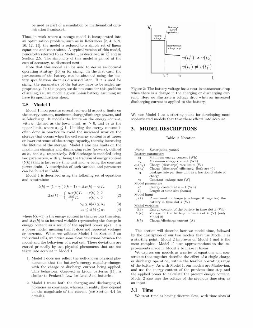
where b(k−1) is the energy content in the previous time step,and ∆E(k) is an internal variable representing the change inenergy content as a result of the applied power p(k). It isa power model, meaning that it does not represent voltagesor currents. When we validate Model 1 in Section 5 onindividual cells, we notice some clear deviations between themodel and the behaviour of a real cell. These deviations arecaused primarily by two physical phenomena that are nottaken into account in Model 1.

1. Model 1 does not reflect the well-known physical phe-nomenon that the battery’s energy capacity changeswith the charge or discharge current being applied.This behaviour, observed in Li-ion batteries [14], issimilar to Peukert’s Law for Lead-Acid batteries.

2. Model 1 treats both the charging and discharging ef-ficiencies as constants, whereas in reality they dependon the magnitude of the current (see Section 4.4 fordetails).

V

tt1 t+1 t2

v(t+1 ) ≈ v(t2)

v(t1) != v(t+1 )

Resting voltage

Discharge current

applied at t1

Instantaneous voltage drop

Figure 2: The battery voltage has a near-instantaneous dropwhen there is a change in the charging or discharging cur-rent. Here we illustrate a voltage drop when an increaseddischarging current is applied to the battery.

We use Model 1 as a starting point for developing moresophisticated models that take these effects into account.

3. MODEL DESCRIPTIONS

Table 1: Notation

Name Description (units)Battery parametersa1 Minimum energy content (Wh)a2 Maximum energy content (Wh)

αc(αd) Charge (discharge) rate limits (W)ηc(ηd) Charge (discharge) efficiency. Both are ≤ 1γ1 Leakage rate per time unit as a fraction of state of

chargeγ2 Constant leakage rate (W)

Model parametersU Energy content at k = 1 (Wh)Tu Length of time slot (hours)

Model inputp(k) Power used to charge (discharge, if negative) the

battery in time slot k (W)Model variablesb(k) Energy content of the battery in time slot k (Wh)V (k) Voltage of the battery in time slot k (V) (only

Model 2)I(k) Charge/discharge current (A)

This section will describe how we model time, followedby the description of our two models that use Model 1 asa starting point. Model 2 improves on Model 1 and is themost complex. Model 1∗ uses approximations to the im-provements made in Model 2 to make it linear.

We express our models as a series of equations and con-straints that together describe the effect of a single chargeor discharge operation, within the feasible operating rangeof the battery. As with Model 1, our models are Markovian,and use the energy content of the previous time step andthe applied power to calculate the present energy content.Model 2 also uses the voltage of the previous time step asan input.

3.1 TimeWe treat time as having discrete slots, with time slots of

Time

time slot k time slot k+1

I(k) I(k + 1)b(k) b(k + 1)

V (k + 1)V (k)

k+ (k + 1)− (k + 2)−

Figure 3: Illustration of time slots.

length Tu. For modelling purposes, it is tempting to makethe assumption that all variables, such as voltage V (k), cur-rent I(k), and energy content b(k), are constant within onetime slot, with changes occurring only at the beginning oftime slots. In practice, however, this assumption can intro-duce errors into the way we calculate the power flowing in orout of the battery in each time slot. For example, if we in-crease the discharging rate significantly at the beginning of atime slot, the voltage of a battery has been observed to dropalmost instantly. Figure 2 illustrates this occurrence, whichmakes it clear that to calculate the power used to charge thebattery or drawn from the battery in time slot k, it is moreaccurate to use the voltage at the end of the time slot ratherthan at the beginning. For this reason, we assume that thevoltage is constant in the interval [k+, (k + 1)−], and usethe voltage at the end of time slot k. Thus, we define I(k)to be the current during time slot k, and b(k) and V (k) asthe respective energy content and voltage at the end of thetime slot. This notation is illustrated in the diagram shownin Figure 3.

3.2 Model 2In Model 2, we extend Model 1 to use current (I(k)) and

voltage (V (k)) as (internal) model variables1. We replacethe contant a1 (upper) and a2 (lower) limits on energy con-tent with functions that depend on the current, denoteda1(I) and a2(I). We also replace constant efficiency param-eters ηc and ηd with functions, denoted as ηc(I) and ηd(I)for charging and discharging efficiency, respectively.

The following set of equations and constraints describesModel 2:

b(k) = (1− γ1)b(k − 1) + ∆E(k)− γ2Tu (5)

∆E(k) =

{ηc(I(k))p(k)Tu : p(k) ≥ 0p(k)

ηd(I(k))Tu : p(k) < 0

(6)

V (k) = V (k)∗ (7)

I(K) =p(k)

V (k)(8)

αd ≤ p(k) ≤ αc (9)

a1(I(k)) ≤ b(k) ≤ a2(I(k)) (10)

The inputs to the model are the parameters (γ1, γ2, ηc(I),ηd(I), αc, αd, a1(I), a2(I)), the empirically-derived functionM (described below), as well as the previous energy contentb(k − 1), previous voltage V (k − 1), and input power p(k).The output of the model is the battery energy content b(k).V (k)∗ is an internal variable that is a fixed point of theiterative process described next.

We first estimate the voltage in time slot k using a pre-dicted energy content and the input power. Let M be afunction that maps the energy content and current to the

1Note that Model 2 is still a power-based model.

cell voltage:

V (k) = M(b(k), I(k)) (11)

M can be empirically derived from the reversible capacitycurves obtained from the battery specifications (see Sec-tion 4.3 for details). However, this function alone does notallow us to predict the voltage. Specifically, although thechange in energy level b(k) can be obtained from Eq. 5, itis dependent on I(k), which can be calculated from the fol-lowing equation:

I(k) =p(k)

V (k). (12)

If we follow these calculations, a loop emerges: we need b(k)to calculate V (k), need I(k) to calculate b(k), and need V (k)to calculate I(k). To get around this, we introduce three

new variables V (k), I(k), and b(k) that are the estimatesfor V (k), I(k), and b(k). Given the input p(k), we computethese estimates using the following iterative process, usingthe most recent estimates V (k), I(k), and b(k) in each step:

Step 1: Initiate V (k) as V (k − 1)

Step 2: Calculate I(k) using Eq. 12

Step 3: Calculate b(k) using Eq. 5

Step 4: Calculate V (k) using Eq. 11

Step 5: Repeat Steps 2, 3, and 4 until V (k) converges to afixed point V (k)∗.

In the thousands of cases where we have used this pro-cess, it has converged quite quickly, usually within a fewiterations. The convergence takes only a handful of itera-tions when the initial value is close to the fixed point, whichis why we take the voltage of the previous time slot as aninitial guess to decrease the number of iterations.

Since M is defined only for voltages in the permitted range[Vmin, Vmax], the voltage limits are implicit in M .

Model 2 covers the noticeable shortcomings of Model 1,but at the cost of increased complexity. The ηd, ηc, a1,and a2 functions may not be linear, and the iterative com-putation that implicitly defines V (k)∗ makes it difficult tointegrate this model as part of a larger optimization model.

3.3 Model 1∗Model 1∗ is a simplified version of Model 2. It uses lin-

ear approximations to the implicit and non-linear parts ofModel 2, specifically the recursive voltage estimation, effi-ciency functions, and energy limit functions:

• We approximate the voltage with the nominal voltage.The nominal voltage is different for charging and dis-charging i.e., V (k) = Vnom,c or Vnom,d,∀k, hence thecharging current is approximated as p(k)/Vnom,c anddischarging current as p(k)/Vnom,d.

• The efficiency functions, ηc(I) and ηd(I), are replacedwith constants, as is done in Model 1.

• The energy limit functions, a1(I) and a2(I), are re-placed with linear approximations and become func-tions of p(k).

These approximations trade off accuracy for tractability. Afurther discussion on these approximations can be found inSection 6.2.

The following set of equations and constraints describesModel 1∗:

b(k) = (1− γ1)b(k − 1) + ∆E(k)− γ2Tu (13)

∆E(k) =

{ηcp(k)Tu : p(k) ≥ 0p(k)ηd

Tu : p(k) < 0(14)

αd ≤ p(k) ≤ αc (15)

a1(p(k)

Vnom,d) ≤ b(k) ≤ a2(

p(k)

Vnom,c) (16)

The inputs to the model are the parameters (γ1, γ2, ηc,ηd, αc, αd, a1(I), a2(I), Vnom,c, Vnom,d), b(k− 1), and p(k).The output of the model is the battery energy content b(k).As mentioned, we approximate the functions ηc(I), ηd(I),a1(I), and a2(I) with constants ηc, ηd and lines for a1, a2.

4. DETERMINING PARAMETERSThere are two methods to obtain the values for the pa-

rameters of our models. The first is from the battery spec-ification sheet (spec) that is published by the manufacturerof the battery being modelled, and the second is to use an IVmeasurement trace. We use the Leclanche Li-Titanate cellspecifications document [11] as an example. This documentcontains reversible discharge curves, such as the ones shownin Figure 4, as well as the nominal voltage and impedancevalues. In the spec, charging and discharging rates are of-ten given in terms of current, i.e., C-rate, where 1C is thecurrent at the output of the BMS needed to fully charge ordischarge the battery in 1 hour. For the Li-Titanate cell, 1Ccorresponds to 30 Ampere current.

Unfortunately, the spec may not have all the informationneeded to derive the model parameters. For example, thereversible discharge curves in Figure 4 only have dischargerates up to 2C even though the spec recommends an upperlimit of 4C discharging. Thus, one source of error is due tothe interpolation of these curves for higher rates. Moreover,the spec gives the average parameters for the class of Li-Titanate cells, but each cell has slightly different parameters.This is a second source of spec error.

If a measurement trace for the cell, that is, a trace of bat-tery voltage as a function of a sequence of charge/dischargeoperations, were available, it can be used to obtain modelparameters, as discussed next. These parameters are spe-cific to the cell under test and therefore do not exhibit specerrors.

Thus, obtaining model parameters both from the spec andfrom experimental traces allows us to distinguish betweenmodelling errors and errors due to the spec. In practice,since experimental traces are hard to obtain, our modelswould exhibit the sum of these errors.

In this section, we discuss how to obtain parameter valuesusing both of these methods. The resulting parameter valuesfor a Li-Titanate cell are presented in Table 5 (Appendix) ifthey are constants for Model 1, or in Figures 6, 7, and 8 ifthey are functions.

The parameters for Model 1 and 1∗ need to be representa-tive and will differ based on the operating range over whichthe battery is used. To reflect this, in this paper we take theaverage values in the charging (resp. discharging) operat-

Reversible Capacity (Ah)

Vo

ltag

e (V

)

Figure 4: Reversible discharge capacity for different dis-charge rates from the specification sheet for Li-Titanate [11].

0 1 2 3 4 5

C rate

1.4

1.6

1.8

2

2.2

2.4

2.6

2.8

Vo

lta

ge

Vnom,c

Vnom,d

Vmax

Vmin

Figure 5: Nominal voltages for a Li-Titanate cell.

ing range as our representative values for those parameterswhich are constant approximations to a curve. We use thenotation ‘Model #[x,y]’ to mean “Model #, with parame-ters approximated in the operating range between x and y”,where x is the largest (negative) discharging current, and yis the largest charging current in the operating range. Notethat the models have some parameters in common (αc, αd,ηc, ηd, γ1, γ2); the values for these parameters in the sameoperating range will be identical for each model.

4.1 Nominal voltage: Vnom,c, Vnom,dThe nominal voltages are parameters for Model 1∗. For

a given C-rate, we take the nominal voltage to be the av-erage cell voltage during a full charge or discharge. It canbe easily derived from a reversible capacity curve from thespec, shown in Figure 4, or from measurements. Figure 5shows the nominal voltage for each of the measured C-rates.For model 1∗[x,y]. Vnom,c and Vnom,d are calculated as theaverage of the nominal voltages for the current range [x,0]and [0,y], respectively.

4.2 Energy content limits: a1, a2, a1(.), a2(.)

These parameters represent the lower and upper limitson the energy content. They are constant in Model 1, anddepend on the operating range. In Model 1∗ and Model 2,they are functions of the current. a1 models the fact that thebattery cannot be discharged fully at high discharge currentsdue to the voltage drop, while a2 models mirrored effects ofthe voltage jump when charging the battery.

These functions can be obtained from the voltage vs. re-

0 1 2 3 4 5

C-rate

0

0.2

0.4

0.6

0.8

1

Charg

e fra

ction

a2 from data

a1 from data

a2 from spec

a1 from spec

Figure 6: a1 and a2 as a function of the current for a Li-Titanate cell. Values derived from the measurements tracesas well as the specs are shown. The spec did not show re-versible capacity curves for as large a range as the measure-ment trace.

versible capacity curves such as the ones shown in Figure 4from the spec, or using similar curves obtained from a mea-surement trace that cycles the battery using the range ofcurrents the battery is designed to handle. When the bat-tery voltage reaches Vmin while a high discharge current isapplied, it does not mean that there is no energy in thebattery; rather, it means that the remaining energy can beaccessed only at a lower discharge current. We choose thevalue of a1(I) to be the energy remaining in a battery whenthe voltage reaches Vmin while being discharged with cur-rent I. A similar effect can be seen when charging a battery.We choose the value of a2(I) to be the energy in the bat-tery when the voltage reaches Vmax at current I. Figure 6shows the a1 and a2 curves derived from both the spec andmeasurement traces.

Model 1[x,y] uses the average values for a1 and a2 in thegiven operating range. Model 1∗[x,y] uses linear approxima-tions to the a1 and a2 curves in the given operating range.In this paper, we use the least-squares linear approximationsto the true curves. The curves are a function of the current,which is approximated as p(k)/Vnom,d for discharging. Theresulting a1(p(k)/Vnom,d) for Model 1∗ is:

a1(p(k)

Vnom,d) = m

p(k)

Vnom,d+ i, (17)

where m and i are the parameters of the line that approxi-mates the true a1 curve in the range [x,y]. a2(p(k)/Vnom,c)is obtained in similar fashion.

4.3 Voltage function: MThe function M , which maps energy content and current

to charging or discharging voltage can be approximated us-ing the reversible capacity curves obtained from either thespec or a measurement trace. The curves map ampere-hourcontent and current to voltage, and by taking the product ofthe ampere-hour content and nominal voltage value to getan energy value, we get a good approximation to M . Fig-ure 7 shows the resulting shape of M when derived usingthe reversible capacity curves from the measurement trace.We use a linear interpolation of the available points as ourfunction M , which maps the energy content in the domain[0Wh,72.5Wh] and current in the domain [-5C, 5C] to volt-age in the range [1.5V, 2.7V]. When the specification’s re-versible capacity curves are used, we get M with energycontent in the domain [0Wh, 74.8Wh]current only in the

1.4

1.6

1.8

60

2

0

2.2

Voltage (

V) 2.4

b(k) (Wh)

40 -50

2.6

Current (A)

20 -100

0 -150

Figure 7: M function for discharging currents, derived usingreversible capacity curves from the measurement trace.

0 1 2 3 4 5

C rate

0.85

0.9

0.95

1

Effic

iency

ηd from data

ηc from data

ηd from spec

ηc from spec

Figure 8: Li-Titanate charging/discharging efficiency as afunction of the current, calculated using the impedance valuefrom the spec [11] and compared to what we observe in themeasurement traces.

domain [-2C, 1C] and voltage in the range [1.7V, 2.7V]; thislimitation effects the range of charging and discharging ratesthat we can use to validate our model with spec-derived pa-rameters.

4.4 Efficiency: ηc, ηd, ηc(.), ηd(.)Since ηc and ηd are constant in Model 1[x,y] and 1∗[x,y],

we set ηc and ηd to be the mean efficiency values in theoperating range [x,y].

For Model 2, the efficiency, which we take to be a functionof I, can be calculated by using the impedance value Ri(provided by the spec) in the following calculations:

efficiency =useful power

total power=

I2RLI2(RL +Ri)

.

Substituting RL = V−IRiI

, we get

efficiency = 1− IRiV

=⇒ ηc(I(k)) = 1− I(k)RiV (k)

(18)

For simplicity, instead of V (k) we use the nominal voltageVnom,I for each charging and discharging current, and hence

ηc(I(k)) = 1− I(k)RiVnom,I(k)

(19)

Both charging and discharging efficiency functions can becalculated this way.

A measurement trace can give us the difference betweeninput and output energy in one full cycle, and thus theround-trip efficiency, which is a product of ηc and ηd. Wedescribe how to isolate the efficiency values by fitting thevalues to what we observe in measured data in Appendix B.Figure 8 shows the resulting efficiency function derived froma measurement trace and the spec, using Ri = 2 mOhms.

4.5 Charging/Discharging limits: αc, αdThe specifications give recommended maximum charging

and discharging C-rates. These are converted into αc and αdpower limits by taking the product of the C-rate limits andthe corresponding nominal voltage of the C-rate. If usinga measurement trace to obtain these parameters, αc is setso that it does not exceed the maximum observed chargingpower (the same for αd and discharging power) providedthat the battery was tested at its maximum charging anddischarging rate when the measurements were taken. Inpractice, these limits are enforced by the control componentof the battery which prevents charging and discharging ratesthat would cause damage to the battery2.

4.6 Self-Discharge: γ1, γ2Unfortunately, the self-discharge parameters (γ1, γ2) are

neither included in the spec nor derivable from our availablemeasurement traces. For Li-ion cells, self-discharge is almostnegligible within short-term experiments, making it difficultto validate the effect of self-discharge on our models. Theliterature suggests that the self-discharge of Li-ion batteriesfollows a curve that can be modelled with the parameters weuse, and is less than 3% of the total capacity per month [18,21]. In the evaluation of our models, our longest experimentlasts up to 110 hours over which the effects of self-dischargewould not be noticeable, so we set both γ1 and γ2 to 0.

5. VALIDATIONIn this section, we describe the data we used to compare

our models with measured results from two Li-Titanate andtwo LiFePO4 cells. We also describe the metrics for com-parison, and present our results in the form of figures anderror tables. As discussed earlier, to distinguish between er-rors caused by parameter estimation and errors inherent tothe model, we use parameters both from the spec and frommeasurements.

5.1 Experimental DataThe measurements were performed for two Li-Titanate

and two LiFePO4 energy storage cells under different con-ditions. The Li-Titanate cells [11] have a voltage range of[1.7,2.7] V, and nominal capacity of 30 Ah, although withlow discharging rates a capacity of at least 32.7 Ah is possi-ble. The LiFePO4 cells [1] have a voltage range of [2,3.6]V,and nominal capacity of 1.1 Ah.

We ran a series of lab experiments using BaSyTec XCTSLab battery testing equipment (manufactured by BaSyTecGmbH, Germany), which has a programmable interface forspecifying the charging and discharging processes of a cell,and mimics a battery controller programmed to prevent thebattery voltage from going beyond [Vmin, Vmax]. The equip-

2In the measurement trace we used, the control componentwas bypassed which allowed us to test currents that are be-yond the range recommended by the spec.

ment gives precise measurements of battery voltage and cur-rent. The cells were placed in a Binder MK 53-E2 climatecontrol chamber (Binder GmbH, Germany) during testing.

The experiments that we conducted test the limits of eachsingle-cell battery in terms of both voltage and current bycycling the cell under different currents and recording thecurrent, voltage, and total charge (Ah) every 10 seconds.We also ran experiments using a variable charging and dis-charging profile that reflects how a battery would be usedto provide back-up power in a system with a solar powersource and building load over an 8-hour period, with a mea-surement granularity of 1 second.

In the experiments with the Li-Titanate cell, we allowedthe voltage to drop to 1.5 V, which is lower than the rec-ommended minimum of 1.7 V given by the spec. We werestill able to obtain parameter values for our model by usingthe measurement trace that contains the low voltages. Wecould not use the spec to obtain parameters to model thisbehaviour, and therefore limit the comparison of our modelwith spec parameters to the measured data when the voltagelies in the permissible range.

5.2 State of Charge MetricWe evaluate our models by comparing the state of charge

(SoC) of the test cells with the SoC computed by each model.We define the SoC of a battery at current I to be the usableenergy in the battery divided by the total capacity at thatcurrent. This metric allows us to determine both how accu-rately our models calculate the energy content as well as howclose our models are to limiting the battery to the accept-able voltage range without actually estimating the voltage.Specifically, the SoC in time slot k is calculated as

SoC(k) =b(k)− a1(I(k))

(a2(I(k))− a1(I(k)))(20)

The SoC of a test cell as it is being charged or dischargedcan be inferred by using a set of mappings from measuredvoltage to SoC. Vmin is mapped to an SoC of 0, Vmax ismapped to an SoC of 1, and the measured charge of thebattery is used to calculate SoC as the battery is cycled. Inthis way, we obtain the SoC of each measured cell using themeasurement traces of each cell. Figure 9 shows a sampleof the mappings we used to infer the SoC of one of the mea-sured cells. This SoC is compared with the SoC suggestedby simulating our models using the same charging and dis-charging processes.3

5.3 EvaluationTo evaluate our models, we used two Li-Titanate cells and

two LiFePO4 cells, and cycled them using each cell’s rangeof recommended charge and discharge currents. We thensimulated one of our models using the same charging anddischarging current that were used in our lab experiments,and compared the SoC of the modelled and real single-cellbattery. The inputs b(k−1) and V (k−1) were initialized tobe the observed value in the first time step of the simulation,and each subsequent time step used the modelled values ofthe previous time step as input, which can potentially causean accumulation of errors. Each case study differs in (a)

3The exception to this is when our modelled cell would havebeen overcharged or undercharged using the power valuesfrom the measurement traces, in which case we clip thepower to prevent this from happening.

Voltage1.4 1.6 1.8 2 2.2 2.4 2.6 2.8

SoC

0

0.2

0.4

0.6

0.8

1

OCV1C2C5C

Figure 9: Experimentally-derived Voltage-SoC mapping fora Li-Titanate cell discharged at various C-rates, as well asat Open Cell condition (OCV).

the model we simulate, (b) how we derived the parameters,(c) the cell chemistry, and (d) the type of charging and dis-charging that we test. We calculated the average residualat each C-rate separately, to give a sense of the range wherethe models perform well and where they do not.

Due to limitations of space, although we studied signifi-cantly more, we can only describe eight case studies in Ta-ble 2, and present the results in Table 3 by showing themean residual between measured and modelled SoC, aver-aged from the two cells of the technology being used in thecase study. In each of the case studies, we compare themeasured and modelled energy content for each chargingand discharging current, which lasts 2-3 cycles. This is doneto isolate the errors at each charging/discharging rate be-ing tested. Case studies E0-E7 look at how variations inthe discharging current affect the modelling of Li-Titanatecells, whose a1 bound changes significantly with the dis-charge current, and the corresponding errors in Table 3 arefor discharging C-rates. Case study E8 looks at how varia-tions in the charging current affect the modelling accuracyof the LiFePO4 cells, whose a2 bound changes significantlywith the charge current, so the errors for E8 in Table 3 aregiven for charging C-rates.

Figure 10 shows the results of case studies E1 and E3. Forclarity, we choose to represent the rest of our results in termsof the residual, which is the absolute difference between SoCobserved in the real cell and the modelled SoC. We show theresiduals from one of the cells in each of the eight case studiesin Table 4. In these figures, E0-E7 show SoC residual duringdischarging, while E8 shows SoC residual during charging.Residual figures for E1 and E4 feature a dashed line showingthe extent of the operating range over which the parameterswere calibrated in those case studies.

We comment on each case study below.

E0: Model 1 is not accurate for the full operating range [-5C, 5C]. The best accuracy occurs at 3C dischargingbecause the ηd and a1 parameter values (chosen asthe average values of their respective functions in theoperating range) are close to the real values at 3C.

E1: The performance of Model 1 at charge/discharge ratesbelow 1C, with parameters that are calibrated for lowcharging and discharging rates [-1C, 1C], is good.

E2: Model 2 significantly lowers the residual at high dis-charge rates with respect to Model 1. The highestresidual occurs at the first 5C discharge cycle. Uponinspection, it was determined that the voltage during

0 10 20 30 40 50

Time (h)

0

0.2

0.4

0.6

0.8

1

SoC

Measured

Model 1

[-1C,1C]

0.1C 0.5C 1C 2C 3C 4C 5C

0 10 20 30 40 50

Time (h)

0

0.2

0.4

0.6

0.8

1

SoC

Measured

Model 1*

[-5C,5C]

0.1C 0.5C 1C 2C 3C 4C 5C

Figure 10: Comparison of measured SoC with modelled SoC.

this cycle behaves very differently from what we ob-serve during the two other 5C cycles in the experiment.See Section 6 for more details.

E3: Model 1∗ shows a significant improvement over Model1 for higher discharge rates. The a1 parameter here isa linear approximation to the curve used in Model 2(Figure 6), while the efficiency parameters are chosento be the average over the entire range of chargingand discharging. The linear approximations happento be a poor match to the a1 values at 2C, 3C, and 5Cdischarging, which is why the model is less accuratefor these C-rates.

E4: When we restrict the upper limit of discharging cur-rents to 3C rather than 5C when doing a linear fit tothe a1 function and calibrating the efficiency, the accu-racy of Model 1∗ improves significantly for dischargingcurrents up to 3C. This is expected, since approximat-ing over a smaller range should result in parametersthat are closer to the values in that range.

E5-E7: The spec is slightly worse than measured parame-ters at describing cell behaviour for all models. Thebiggest difference in accuracy is seen with Model 1∗.This is because the a2 function derived from the specfor Li-Titanate is not a good match of what we observein the measurements (see Figure 6). This parametererror throws off the accuracy of the charging portionof the experiment and carries over into the errors ob-served during discharging.

E8: Model 1∗ performs exceptionally well for varying chargecurves. This is due to the linear shape of the a1 anda2 functions derived from the LiFePO4 cells.

Additional Case Studies:

• When using Model 1 to model a LiFePO4 cell, theaverage SoC error was less than 3.5% for charging rates

up to 3C and discharging rates up to 5C. Thus Model1 appears to be an adequate model for this technologyup to 3C charging and 5C discharging. The error grewto 7% at 4C charging and 10C discharging, which isallowed by the specification. The accuracy with Model2 and Model 1∗ was outstanding for this cell type (<5% error for all tested rates).

• We also tested a more realistic charge discharge be-haviour with charging from a solar trace and dischargefrom a building load. In this test, we found ≈ 3% SoCresidual for all models, with Model 2 slightly outper-forming Model 1∗, and Model 1∗ slightly outperform-ing Model 1. We find these small discrepancies are dueto the fact that the charging and discharging rates inthis experiment are no higher than 1C.

6. DISCUSSION

6.1 InsightsOur cases studies have given us insights into where our

models perform well and where they do not.Model 1 is error-prone when the charging and discharging

rate significantly impact the usable capacity of the batterybut can perform well if the operating range, i.e., the rangeof charging and discharging rates, of the battery being mod-elled is narrow. With Model 1, parameters should be chosento match the middle of the operating range in order to reducethe average error. Given the limitation of Model 1, deter-mining if existing work that uses this model is invalidatedis not a straightforward task, since the storage technologybeing modelled is not always specified. If the cell technol-ogy is Li-ion, it is also necessary to know the cell chemistry,which, as our experiments have shown, has a significant roleon the accuracy of Model 1.

With Model 2, the largest inaccuracies are observed whenthe voltage changes rapidly, often seen when the battery isnearly full or nearly empty. If our energy content calcu-lation is even 1-2% off, it can cause a domino effect thataffects the estimate of the voltage, which then affects theestimate of the current, which affects the value of a1 and a2functions; this problem is exacerbated if the voltage changessignificantly. However, the usable capacity of the battery isnot just limited by its voltage limits, but also by the con-troller in order to preserve the increase in lifetime of thebattery [16]. This widely recommended approach to bat-tery management would limit the voltage to a range that isnarrower than [Vmin, Vmax] where it does not jump or dropsignificantly, i.e., a range where Model 2 has demonstratedexceptional accuracy.

Model 1∗ performs well when the a1 and a2 functions areroughly linear with respect to the current. As seen in ourcomparison of results from E3 and E4, Model 1∗ performsbetter when the operating range is slightly narrowed, so thatthe linear approximation is accurate, and all our case studiesshow us that Model 1∗ has low errors over a much wideroperating range than Model 1.

We observed that the spec parameters did not reflect bat-tery performance as well as the measured parameters, whichwas an expected result. However, in a battery with manycells, individual differences seen in cells should average out,making the spec more accurate. Thus, the battery errors

would likely be smaller than cell errors; verifying this in-sight is part of our future work.

6.2 Model 1∗ parameter approximationsModel 1 and Model 2 represent two points on an accuracy-

tractability spectrum, with Model 1∗ occupying a middlepoint on this spectrum, because it is more accurate thanModel 1 but more tractable than Model 2, making it moreuseful for a researcher who wishes to integrate a storagemodel into an optimization framework. It is possible to em-ploy different approximations than those we used to obtaina different version of Model 1∗. We discuss our choices next.

6.2.1 Voltage ApproximationIn Model 2, a voltage estimate is an internal parameter

used to estimate I(k), which is the input to the ηd, ηc, a1,and a2 functions. While this model is suitable for simulation,the requirement for iterative computation of V (k)∗ makesit difficult to integrate it into an optimization framework.In Model 1∗, we use one of the two appropriate nominalvoltages, one for charging and one for discharging of thecell, to be the voltage estimates.

6.2.2 Energy Limit ApproximationThe a1 and a2 functions in Model 2 are derived from the

reversible capacity curves, which we use to get a collection ofpoints whose interpolation defines the function. To be usefulin an optimization problem, we would need an analyticalapproximation to the function. In Model 1∗, we decided touse linear approximations because they gave an acceptableapproximation to the set of points.

6.2.3 Efficiency ApproximationA primary contributor to the complexity of Model 2 is

the multiplication of the efficiency functions by the inputpower. In many optimization models, the operation of thebattery, i.e., the charging/discharging power, is a variable.The multiplication of the power by the efficiency, which is afunction of the input power, creates a non-linear constraint.To keep the constraint linear, Model 1∗ uses constant ηdand ηc values. We could use a linear approximation for theefficiency, as suggested by Figure 8, if the improved accuracyis worth sacrificing the linearity of the model.

6.3 LimitationsAlthough our models demonstrate a trade off between fi-

delity and complexity, we are aware that they are far fromperfect. We do not take into account several factors thatmay influence the behaviour of a Li-ion battery, such asstate of health and temperature effects which are known tolimit the available capacity of the battery [3, 19]. We do notmodel the internal state of the battery in any detail, whichmeans that we may be missing the opportunity to modelsome key behaviours that would improve the accuracy with-out sacrificing the simplicity of our models. We have notstudied the scaling behaviour of our models for multi-cellbatteries; this is future work.

7. CONCLUSIONSAny model for Li-ion storage must make a tradeoff be-

tween accuracy and tractability, when used as part of anoptimization problem. We have evaluated three differentmodels that make different trade-offs. We find that a model

Table 2: Description of Case Studies

CaseStudy

ModelParameterSource

CellChemistry

Description

E0 1[-5C,5C] Measured Li-TitanateCell is charged at 1C and discharged at a constant rate

between 0.1 and 5C in each cycle.E1 1[-1C,1C] Measured Li-Titanate “”E2 2 Measured Li-Titanate “”E3 1∗[-5C,5C] Measured Li-Titanate “”E4 1∗[-3C,3C] Measured Li-Titanate “”

E5 1[-2C,1C] Spec Li-TitanateCell is charged at 1C and discharged at a constant rate

between 0.1 and 2C in each cycle.E6 2 Spec Li-Titanate “”E7 1∗[-2C,1C] Spec Li-Titanate “”

E8 1∗[-10C,4C] Measured LiFePO4Cell is discharged at 1C and charged at a constant rate

between 0.5 and 4C in each cycle.

Table 3: Average Residual SoC (%).

Case Study 0.1C 0.5C 1C 2C 3C 4C 5CE0 17.7 14.3 12.9 9.3 1.7 16.5 32.0E1 5.4 1.2 1.8 5.2 12.3 25.9 38.0E2 3.0 3.5 4.1 4.0 4.8 7.5 7.0E3 6.9 7.6 8.1 9.7 9.4 7.0 15.8E4 4.9 3.7 3.0 2.7 3.4 15.2 28.0E5 4.2 1.3 2.6 6.4 - - -E6 2.3 2.2 3.7 3.6 - - -E7 3.1 2.4 2.8 3.2 - - -E8 - 0.8 0.9 0.5 1.1 1.1 -

Table 4: State of Charge Residual Figures

0

0.2

0.4

0.6

0.8

1

SoC

Resid

ual

E0

0.1C 0.5C 1C 2C 3C 5C4C0

0.2

0.4

0.6

0.8

1

SoC

Resid

ual

E1

0.1C 0.5C 1C 2C 3C 4C5C0

0.2

0.4

0.6

0.8

1

SoC

Resid

ual

0.1C 0.5C 1C 2C 3C 5C4C

E2

0

0.2

0.4

0.6

0.8

1

SoC

Resid

ual

0.1C 0.5C 1C 2C 3C 5C4C

E3

0

0.2

0.4

0.6

0.8

1

SoC

Resid

ual

0.1C 0.5C 1C 2C 3C 5C4C

E4

0

0.2

0.4

0.6

0.8

1

SoC

Resid

ual

E5

0.1C 0.5C 1C 2C

0

0.2

0.4

0.6

0.8

1

SoC

Resid

ual

0.1C 0.5C 1C 2C

E6

0

0.2

0.4

0.6

0.8

1

SoC

Resid

ual

0.1C 0.5C 1C 2C

E7

0

0.2

0.4

0.6

0.8

1

SoC

Resid

ual

E8

0.5C 1C 2C 3C 4C

that is commonly used in optimization problems to modelstorage systems (Model 1) is too simple to accurately modelthe state of charge of a battery over a wide operating range.Instead we presented a new model (Model 2) that is accurateover a much wider operating range, but is difficult to incor-porate into an optimization problem. We then approximateparts of Model 2 to get Model 1∗, which is simple enough tobe incorporated into an optimization framework while beingaccurate over a significantly wider operating range compared

to Model 1. We believe that our Model 1* is a good balancebetween accuracy and tractability, and is suitable for use ina variety of optimization problems involving energy systems.

In future work, we plan to compare cell error and batteryerror when using spec parameters, and to use Model 1* forsolving a variety of optimization problems. We also wouldlike to better model the state of health of the battery, asfundamental knowledge about this issue is gleaned.

8. REFERENCES[1] A123 Systems. High Power Lithium Ion

APR18650M1A, 2009. LiFePO4 cell specifications.

[2] K. M. Chandy, S. H. Low, U. Topcu, and H. Xu. Asimple optimal power flow model with energy storage.In Decision and Control (CDC), 2010 49th IEEEConference on, pages 1051–1057. IEEE, 2010.

[3] D. Doerffel and S. A. Sharkh. A critical review of usingthe Peukert equation for determining the remainingcapacity of Lead-acid and Lithium-ion batteries.Journal of Power Sources, 155(2):395–400, 2006.

[4] N. Gast, J.-Y. Le Boudec, A. Proutiere, and D.-C.Tomozei. Impact of storage on the efficiency andprices in real-time electricity markets. In Proceedingsof the fourth international conference on Future energysystems, pages 15–26. ACM, 2013.

[5] Y. Ghiassi-Farrokhfal, F. Kazhamiaka, C. Rosenberg,and S. Keshav. Optimal design of solar PV farms withstorage. Sustainable Energy, IEEE Transactions on,6(4):1586–1593, 2015.

[6] Y. Ghiassi-Farrokhfal, S. Keshav, and C. Rosenberg.Toward a realistic performance analysis of storagesystems in smart grids. Smart Grid, IEEETransactions on, 6(1):402–410, 2015.

[7] H. He, R. Xiong, and J. Fan. Evaluation ofLithium-ion battery equivalent circuit models for stateof charge estimation by an experimental approach.Energies, 4(4):582–598, 2011.

[8] X. Hu, S. Li, and H. Peng. A comparative study ofequivalent circuit models for Li-ion batteries. Journalof Power Sources, 198:359–367, 2012.

[9] R. Huang, S. H. Low, U. Topcu, K. M. Chandy, andC. R. Clarke. Optimal design of hybrid energy systemwith PV/wind turbine/storage: A case study. InSmart Grid Communications (SmartGridComm),2011 IEEE International Conference on, pages511–516. IEEE, 2011.

[10] F. Kazhamiaka, C. Rosenberg, and S. Keshav.Practical strategies for storage operation in energysystems: design and evaluation. Accepted to IEEETransactions on Sustainable Energy, 2016.

[11] Leclanche. LecCell 30Ah High Energy, 02 2014.Lithium-Titanate cell specifications.

[12] A. Mishra, R. Sitaraman, D. Irwin, T. Zhu, P. Shenoy,B. Dalvi, and S. Lee. Integrating energy storage inelectricity distribution networks. In Proceedings of the2015 ACM Sixth International Conference on FutureEnergy Systems, pages 37–46. ACM, 2015.

[13] B. Nykvist and M. Nilsson. Rapidly falling costs ofbattery packs for electric vehicles. Nature ClimateChange, 5(4):329–332, 2015.

[14] N. Omar, P. V. d. Bossche, T. Coosemans, and J. V.Mierlo. Peukert revisited – critical appraisal and needfor modification for Lithium-ion batteries. Energies,6(11):5625–5641, 2013.

[15] J. Qin, Y. Chow, J. Yang, and R. Rajagopal.Modeling and online control of generalized energystorage networks. In Proceedings of the 5thinternational conference on Future energy systems,pages 27–38. ACM, 2014.

[16] P. Ramadass, B. Haran, P. M. Gomadam, R. White,and B. N. Popov. Development of first principles

capacity fade model for Li-ion cells. Journal of TheElectrochemical Society, 151(2):A196–A203, 2004.

[17] K. A. Smith, C. D. Rahn, and C.-Y. Wang. Controloriented 1d electrochemical model of Lithium ionbattery. Energy Conversion and Management,48(9):2565–2578, 2007.

[18] M. Swierczynski, D.-I. Stroe, A.-I. Stan,R. Teodorescu, and S. K. Kaer. Investigation on theself-discharge of the lifepo4/c nanophosphate batterychemistry at different conditions. In TransportationElectrification Asia-Pacific (ITEC Asia-Pacific), 2014IEEE Conference and Expo, pages 1–6. IEEE, 2014.

[19] J. Vetter, P. Novak, M. Wagner, C. Veit, K.-C. Moller,J. Besenhard, M. Winter, M. Wohlfahrt-Mehrens,C. Vogler, and A. Hammouche. Ageing mechanisms inLithium-ion batteries. Journal of power sources,147(1):269–281, 2005.

[20] S. S. Zhang. The effect of the charging protocol on thecycle life of a Li-ion battery. Journal of power sources,161(2):1385–1391, 2006.

[21] A. H. Zimmerman. Self-discharge losses in lithium-ioncells. Aerospace and Electronic Systems Magazine,IEEE, 19(2):19–24, 2004.

APPENDIXA. PARAMETER TABLE

Table 5: Model 1[-1C,1C] Li-Titanate parameter values fromspecifications and measurements.

Parameter Spec Measureda1 4 Wh 3.9 Wha2 74 Wh 71.9 Whαc 4C 5Cαd 4C 5Cηc 0.981 0.975ηd 0.974 0.967γ1, γ2 N/A N/A

B. CALCULATING EFFICIENCY FROMMEASUREMENT TRACE

A measurement trace can be used to calculate the differ-ence between input and output energy in one full cycle, giv-ing us the round-trip efficiency which is a product of ηc andηd. To separate the values, we make two assumptions andusing the characteristics of our trace to isolate the efficienciesat different C-rates. We make the following assumptions:

1. The charging efficiency at 1C is some value X.

2. The amount of energy that is used to charge the bat-tery after efficiency losses are accounted for is equalto the amount of energy discharged from the battery(including the losses due to efficiency).

The first assumption gives us a starting point from whichto calculate the rest of the efficiency values, and is a guess forthe true efficiency at 1C. A good guess for Li-Titanate couldbe X = 0.97, which is the efficiency value given by Eq. 19 at1C, although we found that X ≈ 0.96 better reflects whatwe observe in the trace.

For assumption 2 to hold, the energy content of the bat-tery should be the same for when the cycle starts (first charg-ing step) and when it ends (last discharging step), whichholds if the preceding cycle was charged/discharged usingthe same currents. Assumption 2 can be expressed usingthe following equation:

ηc · TotalChargingEnergy =TotalDischargingEnergy

ηd(21)

This equation can be rearranged to isolate ηc or ηd.The measurement trace be used to calculate the total dis-

charging and charging energy, but we are left with two un-knowns (ηc, ηd). These could be isolated by using a particu-lar measurment trace in combination with assumption one.We require a trace that keeps the charging rate constant at1C, and varies the discharging rate. By fixing a value forηc at 1C via assumption 1, we can use Eq. 21 to get thedischarging efficiencies for discharge rates that cover the fulloperating range of the battery. We then use a second tracewhere the charging rate varies and discharging is always ata constant rate. We use Eq. 21 and the newly calculatedηd values to isolate the charging efficiency for charging ratesof the full operating range. The values we obtain throughthis approach end up being very close to the values obtained

from the spec, suggesting that the spec is enough to get agood estimate of the efficiency functions.