mathserver.neu.edumathserver.neu.edu/~levine/publ/ihessummermotives.pdf · six lectures on motives...

SIX LECTURES ON MOTIVES

MARC LEVINE

Preface

These lecture notes are taken from my lecture series in the Asian-French summerschool on motives and related topics. My goal in my lectures was two-fold: to givefirst of all a sketch of Voevodsky’s foundational construction of the triangulatedcategory of motives and its basic properties, and then to give an idea of some of theapplications and wider vistas this construction has made possible. In doing this,wanted also to point out some of the origins of this theory, coming from both thecategorical side involving aspects of sheaf theory and triangulated categories, as wellas the input from algebraic geometry, mainly through algebraic cycles. This latteraspect lead me to devote an entire lecture to so-called moving lemmas, as I felt thissubject captured much of the geometric side of the theory. I also reviewed much ofthe necessary material about triangulated categories and sheaves on a Grothendiecksite, with the intention of making the discussion as accessible as possible.

I chose mixed Tate motives for illustrating applications,. This subject toucheson a broad range of subjects, including the theory of t-structures, Tannakian cat-egories, rational homotopy theory, Grothendieck-Teichmuller theory, moduli ofcurves, polylogarithms and multiple zeta values. For this reason, I felt that anoverview would be of interest to a fairly wide audience. I have also included twolectures on the extension of motives given by the motivic stable homotopy categoryof Morel-Voevodsky, giving a sketch of the construction as well as a discussion ofthe motivic Postnikov tower.

I have made only minor changes and additions to my original lectures in thesenotes; I hope this will transmit the informal nature of the lectures to the reader.The rewriting of these notes let me recall how much I enjoyed the summer school atthe I.H.E.S and gives me the opportunity of thanking most heartily the organizersof summer school, Jean-Marc Fontaine and Jean-Benoit Bost, for putting togethera truly worthwhile conference.

Marc LevineEssen, December 2006

The author thanks the I.H.E.S. and the Universite Paris-Sud 11 at Orsay, as well as the NSF(grant DMS-DMS-0457195), for their financial support.

1

2 MARC LEVINE

Contents

Preface 1

Lecture 1. Triangulated categories of motives 31. Triangulated categories 42. Geometric motives 93. Sites and sheaves 154. Motivic complexes 175. The localization theorem 196. The embedding theorem 23

Lecture 2. Motives and cycle complexes 267. Basic structures in DM eff

gm(k) 268. Cycle complexes and bivariant cycle cohomology 299. Motives of schemes of finite type 3610. Morphisms and cycles 3911. Duality 42

Lecture 3. Mixed Tate motives 4512. Mixed Tate motives in DMgm(k) 4513. The motivic Hopf algebra and Lie algebra 4914. Mixed Tate motives as cycle modules 5115. The action of Gal(Q) on π1(P1 \ S) 5616. Multiple zeta values and periods of mixed Tate motives 60

Lecture 4. Moving Lemmas 6417. Chow-type moving lemma 6418. Friedlander-Lawson: moving in families 6719. Voevodsky’s moving lemma 7020. Suslin’s moving lemma 7321. Bloch’s moving lemma 74

Lecture 5. An introduction to motivic homotopy theory 7922. A bird’s-eye view of classical homotopy theory 7923. Motivic homotopy theory: a quick overview 8724. The unstable motivic homotopy category 8825. T -spectra and the motivic stable homotopy category 91

Lecture 6. The Postnikov tower in motivic stable homotopy theory 9726. Classical Postnikov towers 9727. The motivic Postnikov tower 9828. S1-spectra 9929. The homotopy coniveau tower 10230. The T -stable theory 108References 110

SIX LECTURES ON MOTIVES 3

Lecture 1. Triangulated categories of motives

Our goal in this lecture is to construct a category of motives that should capturethe fundamental properties and structures of a reasonable cohomology theory onsmooth varieties over a field k. To guide the construction, we ask the rather vaguequestion: what kind of structures does “cohomology” have? Al the very least, oneshould have

(1) Pull-back maps f∗ : H∗(Y )→ H∗(X) maps f : X → Y .(2) Products H∗(X)×H∗(Y )→ H∗(X × Y )(3) Some long exact sequences: for example, Mayer-Vietoris for (Zariski) open

covers.(4) Some isomorphisms, for example H∗(X) ∼= H∗(X × A1).

Next, what categorical constructions will lead to all these structures?, First of all,there is an algebraic machinery for generating long exact sequences and imposingisomorphisms, namely the machinery of triangulated categories. This structure isa result of axiomatizing the basic example of the derived category of an abeliancategory. For example, if one considers the abelian category ShvT of sheaves ofabelian groups on a topological space T , then the sheaf cohomology H∗(T,A) withcoefficients in an abelian group A is given as the Ext-group

Hn(T,A) ∼= ExtnShvT

(ZT , AT ),

where ZT , AT are the constant sheaves with value Z, A. In the derived categoryD(ShvT ), one has the canonical isomorphism

Extn(ZT , AT ) ∼= HomD(ShvT )(ZT , AT [n]).

All the well-known long exact sequences for cohomology, such as the Mayer-Vietorissequence, or the Bockstein sequence, arise from the long exact sequence machineryencoded in the triangulated category D(ShvT ). In a general triangulated categoryD, one can define the cohomology of an object X with values in another object Aby

Hn(X, A) := HomD(X, A[n]);

we shall see how the triangulated structure in D gives rise to lots of long exactsequence. This formal view of cohomology has proven extremely valuable in manyareas of mathematics.

The product in cohomology comes from a tensor structure in the triangulatedcategory D, namely a bi-functor

⊗D : D ×D → D

with certain exactness properties. If our coefficent group A has a multiplicationA ⊗ A → A and our object X has a “diagonal” δ : X → X ⊗X, then our formalcohomology becomes a ring via

HomD(X, A[n])⊗Z HomD(X, A[m]) ⊗D−−→ HomD(X ⊗X, A[n + m])δ∗−→ HomD(X, A[n + m]).

We need some geometric input to feed this machine, coming from algebraiccycles. Finally, to understand what comes out of this construction, we need the

4 MARC LEVINE

homological algebra of sheaf theory. Schematically, we have the following picture:

Triangulated tensor categories

((QQQQQQQQQQQQQQQQQQQQQQ

Algebraic cycles // Motives

Sheaf theory

66mmmmmmmmmmmmmmmmmmmmmm

1. Triangulated categories

1.1. Translations and triangles.

Definition 1.1. A translation on an additive category A is an equivalence T :A → A. We write X[1] := T (X). An additive functor F : A → B betweenadditive categories with translation is graded if F (X[1]) = (FX)[1] and similarlyfor morphisms.

Let A be an additive category with translation. A triangle (X, Y, Z, a, b, c) in Ais the sequence of maps

Xa−→ Y

b−→ Zc−→ X[1].

A morphism of triangles

(f, g, h) (X, Y, Z, a, b, c)→ (X ′, Y ′, Z ′, a′, b′, c′)

is a commutative diagram

Xa //

f

Y

g

b // Z

h

c // X[1]

f [1]

X ′a′

// Y ′b′

// Z ′c′

// X ′[1].

1.2. Triangulated categories. Verdier [47] has defined a triangulated category asan additive category A with translation, together with a collection E of triangles,called the distinguished triangles of A, which satisfy

TR1 E is closed under isomorphism of triangles.A

id−→ A→ 0→ A[1] is distinguished.Each X

u−→ Y extends to a distinguished triangle

Xu−→ Y → Z → X[1]

TR2 Xu−→ Y

v−→ Zw−→ X[1] is distinguished ⇔ Y

v−→ Zw−→ X[1]

−u[1]−−−→ Y [1] isdistinguished.


TR3 Given a commutative diagram with distinguished rows

Xu //

f

Yv //

g

Zw // X[1]

Xu′

// Y ′v′

// Zw′

// X[1]

there exists a morphism h : Z → Z ′ such that (f, g, h) is a morphism of triangles:

Xu //

f

Yv //

g

Zw //

h

X[1]

f [1]

Xu′

// Y ′v′

// Zw′

// X][1]

TR4 If we have three distinguished triangles (X, Y, Z ′, u, i, ∗), (Y,Z,X ′, v, ∗, j), and(X, Z, Y ′, w, ∗, ∗), with w = v u, then there are morphisms f Z ′ → Y ′, g Y ′ → X ′

such that

• (idX , v, f) is a morphism of triangles• (u, idZ , g) is a morphism of triangles• (Z ′, Y ′, X ′, f, g, i[1] j) is a distinguished triangle.

A graded functor F : A → B of triangulated categories is called exact if F takesdistinguished triangles in A to distinguished triangles in B.

Remark 1.2. Suppose (A, T, E) satisfies (TR1), (TR2) and (TR3). If (X, Y, Z, a, b, c)is in E , and A is an object of A, then the sequences

. . .c[−1]∗−−−−→ HomA(A,X) a∗−→ HomA(A, Y ) b∗−→

HomA(A,Z) c∗−→ HomA(A,X[1])a[1]∗−−−→ . . .

and

. . .a[1]∗−−−→ HomA(X[1], A) c∗−→ HomA(Z,A) b∗−→

HomA(Y,A) a∗−→ HomA(X, A)c[−1]∗−−−−→ . . .

are exact. This yields:

• (five-lemma): If (f, g, h) is a morphism of triangles in E , and if two of f, g, hare isomorphisms, then so is the third.• If (X, Y, Z, a, b, c) and (X, Y, Z ′, a, b′, c′) are two triangles in E , there is an

isomorphism h : Z → Z ′ such that

(idX , idY , h) (X, Y, Z, a, b, c)→ (X, Y, Z ′, a, b′, c′)

is an isomorphism of triangles.

6 MARC LEVINE

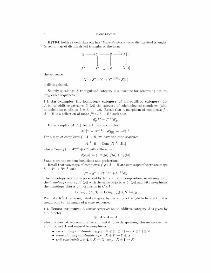
If (TR4) holds as well, then one has “Mayer-Vietoris”-type distinguised triangles:Given a map of distinguished triangles of the form

X //

Y //

Zβ

// X[1]

X ′ // Y ′α

// Z // X ′[1]

the sequence

X → X ′ ⊕ Y → Y ′ βα−−→ X[1]is distinguished.

Shortly speaking: A triangulated category is a machine for generating naturallong exact sequences.

1.3. An example: the homotopy category of an additive category. LetA be an additive category, C?(A) the category of cohomological complexes (withboundedness condition ? = ∅,+,−, b). Recall that a morphism of complexes f :A→ B is a collection of maps fn : An → Bn such that

dnBfn = fn+1dn

A.

For a complex (A, dA), let A[1] be the complex

A[1]n := An+1; dnA[1] := −dn+1

A .

For a map of complexes f : A→ B, we have the cone sequence

Af−→ B

i−→ Cone(f)p−→ A[1]

where Cone(f) := An+1 ⊕Bn with differential

d(a, b) := (−dA(a), f(a) + dB(b))

i and p are the evident inclusions and projections.Recall that two maps of complexes f, g : A→ B are homotopic if there are maps

hn : An → Bn−1 withfn − gn = dn−1

B hn + hn+1dnA

The homotopy relation is preserved by left and right composition, so we may formthe homotopy category K?(A) with the same objects as C?(A) and with morphismsthe homotopy classes of morphisms in C?(A):

HomK?(A)(A,B) := HomC?(A)(A,B)/htpy.

We make K?(A) a triangulated category by declaring a triangle to be exact if it isisomorphic to the image of a cone sequence.

1.4. Tensor structure. A tensor structure on an additive category A is given bya bi-functor

⊗ : A×A → Awhich is associative, commutative and unital. Strictly speaking, this means one hasa unit object 1 and natural isomorphisms

• associativity constraints αX,Y,Z : X ⊗ (Y ⊗ Z)→ (X ⊗ Y )⊗ Z• commutativity constraints τX,Y : X ⊗ Y → Y ⊗X• unit constraints µX,`1⊗X → X, µX,r : X ⊗ 1→ X


which make a short list of diagrams commute (see e.g. Mac Lane [32, chapter VII]for details).

Concretely: for X, Y ∈ A, we have X ⊗ Y ∈ A. For f : X1 → X2, g : Y1 → Y2,we have

f ⊗ g : X1 ⊗ Y1 → X2 ⊗ Y2,

bilinear in f and g and respecting composition:

(f ⊗ g) (f ′ ⊗ g′) = (f f ′)⊗ (g g′).

If A has a translation X 7→ TX =: X[1], we say the tensor structure is graded if(1) T (−⊗−) = T (−)⊗−, T 2(−)⊗− = −⊗T 2(−) as functors A×A → A, i.e.

TX ⊗ Y = T (X ⊗ Y ), T 2X ⊗ Y = X ⊗ T 2Y , and similarly for morphisms,(2) The natural isomorphism τX,Y : X ⊗ TY → TX ⊗ Y

X ⊗ TY ∼= TY ⊗X = T (Y ⊗X) ∼= T (X ⊗ Y ) = TX ⊗ Y

satisfies: T (τX,TY )τX,TY : X ⊗ T 2Y → T 2(X ⊗ Y ) = X ⊗ T 2Y is theidentity.

Definition 1.3. Suppose A is both a triangulated category and a tensor category(with tensor operation ⊗) such that ⊗ is graded.

Suppose that, for each distinguished triangle (X, Y, Z, a, b, c), and each W ∈ A,the sequence

X ⊗Wa⊗idW−−−−→ Y ⊗W

b⊗idW−−−−→ Z ⊗Wc⊗idW−−−−→ X[1]⊗W = (X ⊗W )[1]

is a distinguished triangle. Then A is a triangulated tensor category.

Example 1.4. If A is a tensor category, then K?(A) inherits a tensor structure, bythe usual tensor product of complexes, and becomes a triangulated tensor category.(For ? = ∅, Amust admit infinite direct sums for the tensor structure to be defined).

Giving a tensor structure on an additive category is just giving a natural externalproduct to the Hom-groups; in a triangulated tensor category D the operation f⊗−is compatible with the long exact sequences arising from Hom into or Hom from adistinguished triangle.

1.5. Thick subcategories. The process of Verdier localization allows one to buildnew triangulated categories from old ones by inverting a chosen set of morphismsor equivalently, killing a chosen set of objects.

Definition 1.5. A full triangulated subcategory B of a triangulated category A isthick if B is closed under taking direct summands.

If B is a thick subcategory of A, the set of morphisms s X → Y in A which fitinto a distinguished triangle X

s−→ Y −→ Z −→ X[1] with Z in B forms a saturatedmultiplicative system of morphisms.

The intersection of thick subcategories of A is a thick subcategory of A, So, foreach set T of objects of A, there is a smallest thick subcategory B containing T ,called the thick subcategory generated by T .

Remark 1.6. The original definition (Verdier) of a thick subcategory had the con-dition:

Let Xf−→ Y −→ Z −→ X[1] be a distinguished triangle in A, with Z in B. If f

8 MARC LEVINE

factors as Xf1−→ B′ f2−→ Y with B′ in B, then X and Y are in B.

This is equivalent to the condition given above, that B is closed under direct sum-mands in A (cf. Rickard [42]).

1.6. Localization of triangulated categories. Let B be a thick subcategory ofa triangulated category A and let S be the saturated multiplicative system of mapA

s−→ B with “cone” in B.Form the category A[S−1] = A/B with the same objects as A, with

HomA[S−1](X, Y ) = lim→s:X′→X∈S

HomA(X ′, Y ).

Composition of diagrams

Y ′ g//

t

Z

X ′f

//

s

Y

X

is defined by filling in the middle

X ′′ f ′//

s′

Y ′ g//

t

Z

X ′f

//

s

Y

X.

One can describe HomA[S−1](X, Y ) by a calculus of left fractions as well, i.e.,

HomA[S−1](X, Y ) = lim→s:Y→Y ′∈S

HomA(X, Y ′).

Let QB : A → A/B be the canonical functor.

Theorem 1.7 (Verdier). (i) A/B is a triangulated category, where a triangle T inA/B is distinguished if T is isomorphic to the image under QB of a distinguishedtriangle in A.

(ii) The functor QB is universal for exact functors F : A → C such that F (B)is isomorphic to 0 for all B in B.

(iii) S is equal to the collection of maps in A which become isomorphisms in A/Band B is the subcategory of objects of A which becomes isomorphic to zero in A/B.

Remark 1.8. IfA admits some infinite direct sums, it is sometimes better to preservethis property. A subcategory B of A is called localizing if B is thick and is closedunder all direct sums which exist in A.

For instance, if A admits arbitrary direct sums and B is a localizing subcategory,then A/B also admits arbitrary direct sums.


Localization with respect to localizing subcategories has been studied by Thoma-son [46] and by Ne’eman [37], among others.

In concrete situations, one starts with a triangulated category D, such as the ho-motopy category K(A) of an additive category A. One can then choose a collectionof morphisms in D that one would like to invert. Verdier’s localization theoremis applied with the thick subcategory B ⊂ D being the smallest thick subcategorycontaining the “cones” on the chosen morphisms. The localization D → D/B isthen the universal construction for inverting the chosen morphisms in the settingof triangulated categories.

Remark 1.9 (Localization of triangulated tensor categories). If A is a triangulatedtensor category, and B a thick subcategory, call B a thick tensor subcategory if Ain A and B in B implies that A⊗B and B ⊗A are in B.

The quotient QB : A → A/B of A by a thick tensor subcategory inherits thetensor structure, and the distinguished triangles are preserved by tensor productwith an object.

Example 1.10 (The derived category). The classic example is the derived categoryD?(A) of an abelian category A. D?(A) is the localization of the homotopy categoryK?(A) with respect to the multiplicative system of quasi-isomorphisms f : A→ B,i.e., f which induce isomorphisms Hn(f) : Hn(A)→ Hn(B) for all n.

The derived category is the natural place to perform homological algebra in A.For instance, for M,N are in A, there is a natural isomorphism

ExtnA(M.N) ∼= HomD?(A)(M,N [n]).

If A is an abelian tensor category, then D−(A) inherits a tensor structure ⊗L ifeach object A of A admits a surjection P → A where P is flat, i.e. M 7→M ⊗ P isan exact functor on A. If each A admits a finite flat (right) resolution, then Db(A)has a tensor structure ⊗L as well. The tensor structure ⊗L is given by forming foreach A ∈ K?(A) a quasi-isomorphism P → A with P a complex of flat objects inA, and defining

A⊗L B := Tot(P ⊗B).

2. Geometric motives

Voevodsky constructs a number of categories: the category of geometric motivesDMgm(k) with its effective subcategory DM eff

gm(k), as well as a sheaf-theoretic con-struction DM eff

− , containing DM effgm(k) as a full dense subcategory. In contrast to

almost all other constructions of categories of motives, these are based on homologyrather than cohomology as the starting point, in particular, the motives functorfrom Sm/k to these categories is covariant.

In this section, we discuss the construction of the “geometric” categories DM effgm(k)

and DMgm(k).

2.1. Algebraic cycles and rational equivalence.

Definition 2.1. For X ∈ Schk, let zr(X) be the free abelian group on the integralclosed subschemes of X of dimension r over k We write z∗(X) for the graded group⊕rzr(X). An element Z =

∑i niZi of z(X) is an algebraic cycle on X.

10 MARC LEVINE

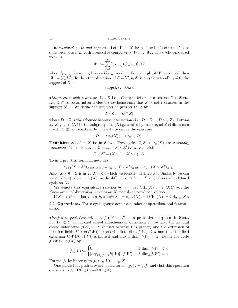
•Associated cycle and support. Let W ⊂ X be a closed subscheme of puredimension n over k, with irreducible components W1, . . . ,Wr. The cycle associatedto W is

|W | :=r∑

i=1

[`OX,Wi(OW,Wi

)] ·Wi

where `OX,Wiis the length as an OX,Wi

module. For example, if W is reduced, then|W | =

∑i Wi. In the other direction, if Z =

∑i niZi is a cycle with all ni 6= 0, the

support of Z isSupp(Z) := ∪iZi.

•Intersection with a divisor. Let D be a Cartier divisor on a scheme X ∈ Schk.Let Z ⊂ X be an integral closed subscheme such that Z is not contained in thesupport of D. We define the intersection product D · Z by

D · Z := |D ∩ Z|where D ∩ Z is the scheme-theoretic intersection (i.e. D ∩ Z := D ×X Z). Lettingzn(X)D ⊂ zn(X) be the subgroup of zn(X) generated by the integral Z of dimensionn with Z 6⊂ D, we extend by linearity to define the operation

D · − : zn(X)D → zn−1(D).

Definition 2.2. Let X be in Schk. Two cycles Z,Z ′ ∈ zn(X) are rationallyequivalent if there is a cycle Z ∈ zn+1(X × A1)X×0+X×1 with

Z − Z ′ = (X × 0−X × 1) · Z.

To interpret this formula, note that

zn+1(X × A1)X×0+X×1 = zn+1(X × A1)X×0 ∩ zn+1(X × A1)X×1.

Also (X × 0) · Z is in zn(X × 0), which we identify with zn(X). Similarly we canview (X × 1) · Z as in zn(X), so the difference (X × 0−X × 1) · Z is a well-definedcycle on X.

We denote this equivalence relation by ∼r. Set CHn(X) := zn(X)/ ∼r, theChow group of dimension n cycles on X modulo rational equivalence.

If X has dimension d over k, set zn(X) := zd−n(X) and CHn(X) := CHd−n(X).

2.2. Operations. These cycle groups admit a number of operations and functori-alities:

•Projective push-forward. Let f : Y → X be a projective morphism in Schk.For W ⊂ Y an integral closed subscheme of dimension n, we have the integralclosed subscheme f(W ) ⊂ X (closed because f is proper) and the extension offunction fields f∗ : k(f(W )) → k(W ). Note dimk f(W ) ≤ n and that the fieldextension k(W )/k(f(W )) is finite if and only if dimk f(W ) = n. Define the cyclef∗(W ) ∈ zn(X) by

f∗(W ) :=

0 if dimk f(W ) < n

[degk(f(W )) k(W )] · f(W ) if dimk f(W ) = n

Extend f∗ by linearity to f∗ : zn(Y )→ zn(X).One shows that push-forward is functorial: (gf)∗ = g∗f∗ and that this operation

descends to f∗ : CHn(Y )→ CHn(X).


•Pull-back. Let f : Y → X be a morphism in Schk with X smooth over k. Forsimplicity, we suppose X and Y are integral. There is a partially defined pull-backmorphism f∗ : zn(X)f → zn(Y ), where zn(X)f is the subgroup of zn(X) consistingof cycles in good position for f . For W ⊂ X an integral codimension n subscheme,W is in good position if each irreducible component of f−1(W ) has codimension non Y . If Z is an irreducible component of f−1(W ) define the multiplicity m(W,Z; f)by Serre’s formula

m(W,Z; f) :=∑i≥0

(−1)i`OY,Z(TorOX,W

i (OW ,OY,Z));

the fact that X is smooth implies that the sum is finite. Define

f∗(W ) :=∑Z

m(W,Z; f)Z

where the sum is over all irreducible components Z of f−1(W ). Letting zn(X)f bethe subgroup of zn(X) generated by all W in good position for f , we extend bylinearity to define the pull-back f∗ : zn(X)f → zn(Y ).

The fundamental advantage of the quotient CHn is that this partially definedpull-back descends to a well-defined pull-back

f∗ : CHn(X)→ CHn(Y )

which is functorial, (fg)∗ = g∗f∗, if X and Y are both smooth. The case of X quasi-projective was handled by the geometric methods of Chow et. al.; the general caserelies on Fulton’s methods [16], or the K-theoretic approach of Quillen-Grayson [18].

•Products. For X and Y in Schk, we have the external product

: zn(X)⊗ zm(Y )→ zn+m(X ×k Y )

defined as the Z-linear extension of the operation (W,W ′) 7→ |W×kW ′| for W ⊂ X,W ′ ⊂ Y integral of dimensions n, m, respectively. is commutative, associativeand unital (with unit the cycle Spec k ∈ z0(Spec k)). The external product descendsto an external product

: CHn(X)⊗ CHm(Y )→ CHn+m(X ×k Y ).

For X smooth, we have the cup product

∪X : CHn(X)⊗ CHm(X)→ CHn+m(X)

defined bya ∪X b := δ∗(a b)

where δ : X → X × X is the diagonal. This product makes the graded groupCH∗(X) := ⊕nCHn(X) into a commutatve graded ring with unit 1X the class of[X] ∈ CH0(X).

•Compatibilities. Beside the functorialities for pull-back and push-forward, we havethe following identities and compatibilities of maps on CH∗:

(1) For f : Y → X a morphism in Sm/k, f∗ : CH∗(X) → CH∗(Y ) is a ringhomomorphism

12 MARC LEVINE

(2) Let f : Y → X, g : Z → X be morphisms in Sm/k with f projective.Suppose that W := Y ×X Z is smooth of dimension dimY +dim Z−dim X.Consider the cartesian diagram

Wf ′

//

g′

Z

g

Yf

// X

Then f ′ is projective and g∗f∗ = f ′∗g′∗.

(3) Projection formula. Let f : Y → X be a projective morphism in Sm/k.Then for a ∈ CHn(X), b ∈ CHm(Y ), we have

f∗(f∗(a) ∪Y b) = a ∪X f∗(b).

2.3. Correspondences and Chow motives. A cycle of dimension n := dim Xon X × Y defines a correspondence from X to Y .

If X, Y and Z are smooth and projective, we can compose correspondences:α ∈ CHdim X(X × Y ), β ∈ CHdim Y (Y × Z):

β α := pXZ∗(p∗XY (α) · p∗Y Z(β)).

Remark 2.3. Let SmProj/k be the category of smooth projective k-schemes. Forf : X → Y a morphism in SmProj/k, we have the class [Γf ] ∈ CHdim X(X × Y )of the graph of f . One easily checks that for morphisms f : X → Y , g : Y → Z,we have

[Γg] [Γf ] = [Γgf ].

Form the category of Chow correspondences CorCH(k) with objects [X] for X ∈SmProjk, with morphisms

HomCorCH(k)([X], [Y ]) := CHdim X(X × Y )

and composition the commposition of correspondences defined above.Before defining the category of effective Chow motives, we make a brief cate-

gorical detour. Recall that for an additive category A, we call A pseudo-abelianif for each idempotent endomorphism α : M → M , α2 = α, there exist objectsM0,M1 ∈ A and an isomorphism φ : M → M0 ⊕ M1 such that φ α φ−1 =0M0 ⊕ idM1 . Given an arbitrary additive category A, there is an additive functori : A → A\ to a pseudo-abelian category A\ which is universal for additive functorsof A to pseudo-abelian categories. A\ is constructed as follows: The objects of A\

are pairs (M,α) wiht M ∈ A and α : M →M an idempotent endomorphism. Themorphisms are given by

HomA\(M,α), (N, β)) := β f α | f ∈ HomA(M,N)with composition (γ g β) (β f α) := γ (g β f) α. The functor i is givenby i(M) := (M, id). For a pair M,α, the identity maps on M give an isomorphismin A\

(M, id) ∼= (M, 1− α)⊕ (M,α);it is not hard to extend this to show that A\ is pseudo-abelian.

Definition 2.4. The categoryMeff(k) of effective homological Chow motives overk is the pseudo-abelian hull CorCH(k)\ of CorCH(k). Denote the object ([X], id) ofMeff(k) by mCH(X).


Remark 2.5. Sending X ∈ SmProj/k to mCH(X) and f : X → Y to [Γf ] ∈CHdim X(X × Y ) defines a functor

mCH : SmProj/k →Meff(k).

Grothendieck’s original construction of Chow motives is different from the con-struction given here in that the Grothendieck construction uses the correspondencegroup CorCH(X, Y ) := CHdim X(X × Y ) (with the same composition law) insteadof CHdim X(X × Y ). As the graph of a morphism f : X → Y is thus an element[Γf ] ∈ CorCH(Y, X), the analogous construction leads to the category of effectivecohomological motivesMeff(k) and a functor

mCH : Sm/kop →Meff(k)

In the end, the “true” category of Chow motives M(k), formed from Meff(k) byinverting the Lefschetz motive, has a duality operation, so there is no essentialdifference between M(k) and M(k)op. We use the homological formulation to fitwith Voevodsky’s construction of the triangulated category of effective motives.

2.4. Some philosophy. We lose information in the category of motives by makingthe morphisms the rational equivalence classes of cycles. It would be better to usethe cycles themselves, and think of the rational equivalences as homotopies of maps.It would also be nice to have objects in our category for each X ∈ Sm/k ratherthan just the smooth projective ones.

It is however not possible to use our composition formula to give a well-definedoperation

zdim X(X × Y )⊗ zdim Y (Y × Z)→ zdim X(X × Z) :the intersection product is not always defined. Furthermore, if Y is not projective,the projection operation pXZ∗ is not defined.

2.5. Finite correspondences. To solve the problem of the partially defined com-position of correspondences and to extend the composition formula to smooth butnon-projective schemes, Voevodsky introduces the notion of finite correspondences.

Definition 2.6. Let X and Y be in Schk. The group c(X, Y ) is the subgroup ofz(X ×k Y ) generated by integral closed subschemes W ⊂ X ×k Y such that

(1) the projection p1 : W → X is finite(2) the image p1(W ) ⊂ X is an irreducible component of X.

The elements of c(X, Y ) are called the finite correspondences from X to Y .

The following basic lemma is easy to prove:

Lemma 2.7. Take X, Y in Sm/k and Z in Schk, W ∈ c(X, Y ), W ′ ∈ c(Y, Z).Suppose that X and Y are irreducible. Then each irreducible component C ofSupp(W )× Z ∩X × Supp(W ′) is finite over X and pX(C) = X.

Thus: for W ∈ c(X, Y ), W ′ ∈ c(Y, Z), and X, Y, Z ∈ Sm/k, we have thecomposition:

W ′ W := pSXZ∗(p

∗XY (W ) · p∗Y Z(W ′));

where S := Supp(W ) ∩ Supp(W ′) and pSXZ : S → X × Z is the morphism induced

from the projection pXZ . This operation yields an associative bilinear compositionlaw

: c(Y,Z)× c(X, Y )→ c(X, Z).

14 MARC LEVINE

Remark 2.8. In fact, a modification of the formula gives a well-defined composition : c(Y,Z)× c(X, Y )→ c(X, Z) for X, Y ∈ Sm/k, Z ∈ Schk.

2.6. The category of finite correspondences.

Definition 2.9. The category Cor(k) is the category with the same objects asSm/k, with

HomCor(k)(X, Y ) := c(X, Y ),

and with the composition as defined above.

Remarks 2.10. (1) We have the functor Sm/k → Cor(k) sending a morphismf : X → Y in Sm/k to the graph Γf ⊂ X ×k Y . We write the morphism corre-sponding to Γf as f∗, and the object corresonding to X ∈ Sm/k as [X].

(2) The operation ×k (on smooth k-schemes and on cycles) makes Cor(k) a ten-sor category. Thus, the bounded homotopy category Kb(Cor(k)) is a triangulatedtensor category.

2.7. The category of effective geometric motives.

Definition 2.11. The category DMeff

gm(k) is the localization of Kb(Cor(k)), as atriangulated tensor category, by

• Homotopy. For X ∈ Sm/k, invert p∗ : [X × A1]→ [X]

• Mayer-Vietoris. Let X be in Sm/k. Write X as a union of Zariski open sub-schemes U, V : X = U ∪ V . We have the canonical map

Cone([U ∩ V ](jU,U∩V ∗,−jV,U∩V ∗)−−−−−−−−−−−−−→ [U ]⊕ [V ])

(jU∗+jV ∗)−−−−−−−→ [X]

since (jU∗ + jV ∗) (jU,U∩V ∗,−jV,U∩V ∗) = 0. Invert this map.

The category DM effgm(k) of effective geometric motives is the pseudo-abelian hull

of DMeff

gm(k).

The morphisms inverted to form DMeff

gm(k) are closed under ⊗, so DM effgm(k)

inherits the tensor structure ⊗ from Kb(Cor(k)). It follows from the main result of[4] that the pseudo-abelian hull of a triangulated category is a triangulated category.

2.8. The category of geometric motives. To define the category of geometricmotives we invert the Lefschetz motive. For X ∈ Smk, the reduced motive is

[X] := Cone(p∗ : [X]→ [Spec k])[−1].

Set Z(1) := [P1][−2], and set Z(n) := Z(1)⊗n for n ≥ 0.

Definition 2.12. The category of geometric motives, DMgm(k), is defined byinverting the functor ⊗Z(1) on DM eff

gm(k), i.e., one has objects X(n) for X ∈DM eff

gm(k), n ∈ Z and

HomDMgm(k)(X(n), Y (m)) := lim→N

HomDMeffgm(k)(X ⊗ Z(n + N), Y ⊗ Z(m + N)).


Remarks 2.13. (1) Sending X to X(0) and using the canonical map to the limit

HomDMeffgm(k)(X, Y )→ lim→

N

HomDMeffgm(k)(X ⊗ Z(N), Y ⊗ Z(N))

defines the functor i : DM effgm(k)→ DMgm(k). For n ≥ 0, we have the evident map

i(X ⊗ Z(n))→ X(n), which is an isomorphism

(2) In order that DMgm(k) be again a triangulated tensor category, it suffices thatthe commutativity involution Z(1)⊗ Z(1) → Z(1)⊗ Z(1) be the identity, which isin fact the case.

(3) Setting Z(n) := 1(n) for n ∈ Z, we have X(n) ∼= X ⊗ Z(n) and Z(n)⊗ Z(m) ∼=Z(n + m).

(4) We have the functor Mgm : Sm/k → DM effgm sending X to the image of [X] and

f to the image of the graph Γf .

Of course, there arises the question of the behavior of the functor i : DM effgm(k)→

DMgm(k). Here we have the result due to Voevodsky

Theorem 2.14 (Cancellation). The functor i : DM effgm(k) → DMgm(k) is a fully

faithful embedding.

The first proof of this result used resolution of singularities, but the later proofdoes not, and is valid in all characteristics. We will look at the proof of the cancel-lation theorem in more detail, when we consider various cycle complexes.

3. Sites and sheaves

In order to make computations of the morphisms in DM effgm(k), Voevodsky has in-

troduced a parallel sheaf-theoretic construction, leading to the category DM eff− (k).

We begin our discussion of this approach with a quick review of the theory ofsheaves on a Grothendieck site. For a detailed reference, see [3, 1, 2]

3.1. Presheaves. A presheaf P on a small category C with values in a category Ais a functor

P : Cop → A.

Morphisms of presheaves are natural transformations of functors. This defines thecategory of A-valued presheaves on C, PreShvA(C).

Remark 3.1. We require C to be small so that the collection of natural transfor-mations ϑ : F → G, for presheaves F,G, form a set. It would suffice that C beessentially small (the collection of isomorphism classes of objects form a set).

3.2. Structural results.

Theorem 3.2. (1) If A is an abelian category, then so is PreShvA(C), with kerneland cokernel defined objectwise: For f : F → G,

ker(f)(x) = ker(f(x) : F (x)→ G(x));

coker(f)(x) = coker(f(x) : F (x)→ G(x)).

(2) For A = Ab, PreShvAb(C) has enough injectives.

16 MARC LEVINE

The second part is proved by using a result of Grothendieck [19], noting thatPreShvAb(C) has the set of generators ZX | X ∈ C, where ZX(Y ) is the freeabelian group on HomC(Y,X).

3.3. Pre-topologies.

Definition 3.3. Let C be a category. A Grothendieck pre-topology τ on C is givenby: For X ∈ C there is a set Covτ (X) of covering families of X: a covering familyof X is a set of morphisms fα : Uα → X in C. These satisfy:

A1. idX is in Covτ (X) for each X ∈ C.

A2. For fα : Uα → X ∈ Covτ (X) and g : Y → X a morphism in C, thefiber products Uα ×X Y all exist and p2 : Uα ×X Y → Y is in Covτ (Y ).

A3. If fα : Uα → X is in Covτ (X) and if gαβ : Vαβ → Uα is in Covτ (Uα)for each α, then fα gαβ : Vαβ → X is in Covτ (X).

Remark 3.4. We will not define the “correct” notion, that of a Grothendieck topol-ogy. Suffice it to say that a pre-topology generates a topology (although not everytopology arises this way), and that one can define our category of interest, sheaves,directly from a given pre-topology.

A category with a (pre) topology is a site.

Example 3.5. If T is a topological space, let Op(T ) be the category with objectsthe open subsets U ⊂ T and morphisms the inclusions V ⊂ U . Give Op(T ) apre-topology by defining a covering family of U ⊂ T to be a collection of Vα ⊂ Usuch that U = ∪αVα.

But there are more examples than this!

The main difference between a Grothendieck (pre)-topology and the usual notioncoming from classical topology is that we don’t require that an “open” of X, Uα →X be an open subset, but just a morphism in the underlying category. Fiberproduct U ×X V replaces intersection U ∪ V .

3.4. Sheaves on a site. For S presheaf of abelian groups on C and fα : Uα →X ∈ Covτ (X) for some X ∈ C, we have the “restriction” morphisms

f∗α : S(X)→ S(Uα)

p∗1,α,β : S(Uα)→ S(Uα ×X Uβ)

p∗2,α,β : S(Uβ)→ S(Uα ×X Uβ).

Taking products, we have the sequence of abelian groups

(3.4.1) 0→ S(X)Q

f∗α−−−→∏α

S(Uα)Q

p∗1,α,β−Q

p∗2,α,β−−−−−−−−−−−−→∏α,β

S(Uα ×X Uβ).

Definition 3.6. A presheaf S is a sheaf for τ if for each covering family fα : Uα →X ∈ Covτ , the sequence (3.4.1) is exact. The category ShvAb

τ (C) of sheaves ofabelian groups on C for τ is the full subcategory of PreShvAb(C) with objects thesheaves.


Proposition 3.7. (1) The inclusion i : ShvAbτ (C) → PreShvAb

τ (C) admits a leftadjoint: the sheafification functor.

(2) ShvAbτ (C) is an abelian category: For f : F → G, ker(f) is the presheaf kernel.

coker(f) is the sheafification of the presheaf cokernel.

(3) ShvAbτ (C) has enough injectives.

Remark 3.8. For the “classical” pre-topology on Op(T ), T a topological space, werecover the usual notion of a sheaf.

4. Motivic complexes

Voevodsky’s construction of a sheaf-theoretic category of motives mixes togetherthe category of Nisnevich sheaves on Sm/k with presheaves on the larger categoryCor(k), giving the category of “Nisnevich sheaves with transfers”. This is stillnot the correct category, one needs to form the derived category and then pass tothe subcategory of complexes with A1-invariant cohomology to force A1-homotopyinvariance; the Mayer-Vietoris property is already built in.

4.1. Nisnevich sheaves with transfers.

Definition 4.1. Let X be a k-scheme of finite type. A Nisnevich cover U → X isan etale morphism of finite type such that, for each finitely generated field extensionF of k, the map on F -valued points U(F )→ X(F ) is surjective.

Using Nisnevich covers as covering families gives us the small Nisnevich site onX, XNis. The big Nisnevich site over k is defined similarly, except that now theunderlying category is all of Sm/k and for X ∈ Sm/k the covering families of Xare the same as for XNis.

Notation 4.2. ShNis(X) := Nisnevich sheaves of abelian groups on X, ShNis(k) :=Nisnevich sheaves of abelian groups on Sm/k. For a presheaf F on Sm/k or XNis,we let FNis denote the associated sheaf.

For X ∈ Schk, Z(X) denotes the presheaf of abelian groups on Sm/k freelygenerated by HomSchk

(−, X), ZNis(X) the Nisnevich sheaf. PreShNis(Sm/k) hasa tensor product:

(F ⊗G)(X) := F (X)⊗Z G(X)and internal Hom: Hom(F,G)(X) := HomPreShNis(Sm/k)(F ⊗ Z(X), G).

ShNis(Sm/k) has the tensor product by sheafifying the presheaf ⊗. The in-ternal Hom in ShNis(Sm/k) is given by Hom(F,G)(X) := HomShNis(Sm/k)(F ⊗ZNis(X), G).

For F a sheaf, we have the canonical surjection ⊕X,s∈F (X)ZNis(X)→ F . Iterat-ing gives the canonical left resolution LNis(F )→ F .

Definition 4.3. (1) The category PST(k) of presheaves with transfer is the cate-gory of presheaves of abelian groups on Cor(k).

(2) The category of Nisnevich sheaves with transfer on Sm/k, ShNis(Cor(k)), is thefull subcategory of PST(k) with objects those F such that, for each X ∈ Sm/k, therestriction of F to XNis is a sheaf. We have the sheafification functor F 7→ FNis.

18 MARC LEVINE

Remark 4.4. A PST F is a presheaf on Sm/k together with transfer maps

Tr(a) : F (Y )→ F (X)

for every finite correspondence a ∈ Cor(X, Y ), satisfying:

Tr(Γf ) = f∗, Tr(a b) = Tr(b) Tr(a), Tr(a± b) = Tr(a)± Tr(b).

Definition 4.5. Let F be a presheaf of abelian groups on Sm/k. We call Fhomotopy invariant if for all X ∈ Sm/k, the map

p∗ : F (X)→ F (X × A1)

is an isomorphism. We call F strictly homotopy invariant if for all q ≥ 0, thecohomology presheaf X 7→ Hq(XNis, FNis) is homotopy invariant.

Theorem 4.6 (PST [48, chapter 3, thm. 4.27, thm. 5.7]). Let F be a homotopyinvariant PST on Sm/k. Then

(1) The cohomology presheaves X 7→ Hq(XNis, FNis) are PST’s.(2) FNis is strictly homotopy invariant.(3) FZar = FNis and Hq(XZar, FZar) = Hq(XNis, FNis).

Remarks 4.7. (1) uses the fact that for finite map Z → X with X Hensel local and Zirreducible, Z is also Hensel local. (2) and (3) rely on Voevodsky’s generalization ofQuillen’s proof of Gersten’s conjecture, viewed as a “moving lemma using transfers”:

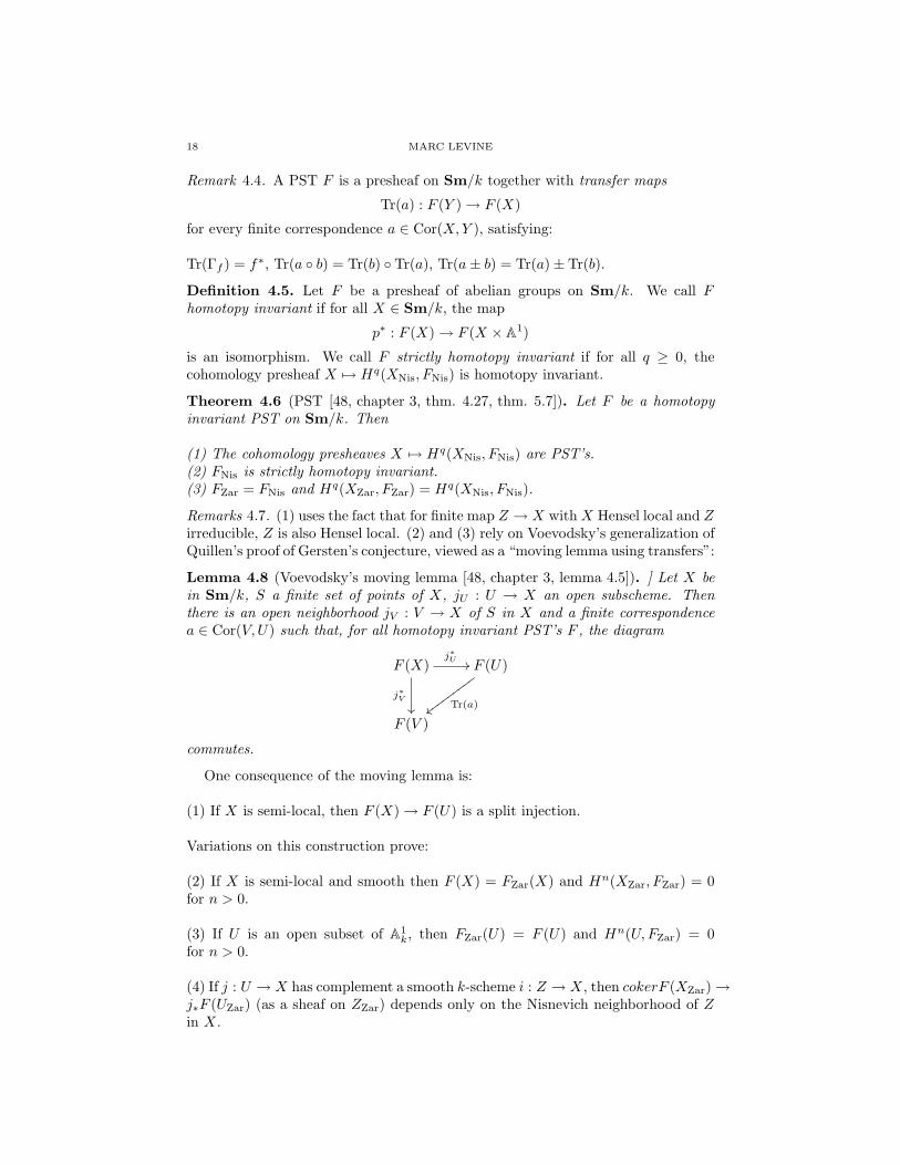
Lemma 4.8 (Voevodsky’s moving lemma [48, chapter 3, lemma 4.5]). ] Let X bein Sm/k, S a finite set of points of X, jU : U → X an open subscheme. Thenthere is an open neighborhood jV : V → X of S in X and a finite correspondencea ∈ Cor(V,U) such that, for all homotopy invariant PST’s F , the diagram

F (X)j∗U //

j∗V

F (U)

Tr(a)ww

wwww

www

F (V )

commutes.

One consequence of the moving lemma is:

(1) If X is semi-local, then F (X)→ F (U) is a split injection.

Variations on this construction prove:

(2) If X is semi-local and smooth then F (X) = FZar(X) and Hn(XZar, FZar) = 0for n > 0.

(3) If U is an open subset of A1k, then FZar(U) = F (U) and Hn(U,FZar) = 0

for n > 0.

(4) If j : U → X has complement a smooth k-scheme i : Z → X, then cokerF (XZar)→j∗F (UZar) (as a sheaf on ZZar) depends only on the Nisnevich neighborhood of Zin X.


(1)-(4) together with some cohomological techniques prove the theorem.

4.2. The category of motivic complexes.

Definition 4.9. Inside the derived category D−(ShNis(Cor(k))), we have the fullsubcategory DM eff

− (k) consisting of complexes whose cohomology sheaves are ho-motopy invariant.

Proposition 4.10. DM eff− (k) is a triangulated subcategory of D−(ShNis(Cor(k))).

This follows from

Lemma 4.11. Let HI(k) ⊂ ShNis(Cor(k)) be the full subcategory of homotopyinvariant sheaves. Then HI(k) is an abelian subcategory of ShNis(Cor(k)), closedunder extensions in ShNis(Cor(k)).

Proof. Proof of the lemma. Given f : F → G in HI(k), ker(f) is the presheafkernel, hence in HI(k). The presheaf coker(f) is homotopy invariant, so by thePST theorem coker(f)Nis is homotopy invariant. Given 0 → A → E → B → 0exact in ShNis(Cor(k)) with A,B ∈ HI(k), consider p : X × A1 → X. The PSTtheorem implies R1p∗A = 0, so

0→ p∗A→ p∗E → p∗B → 0

is exact as sheaves on X. Thus p∗E = E, so E is homotopy invariant.

5. The localization theorem

To understand DM eff− (k) better, we realize it as a localization of D−(ShNis(Cor(k)))

rather than a subcategory.

5.1. The Suslin complex. Let ∆n := Spec k[t0, . . . , tn]/∑n

i=0 ti − 1. n 7→ ∆n

defines the cosimplicial k-scheme ∆∗ with coface maps

δni : ∆n → ∆n+1

the mapδni (x0, . . . , xn) := (x0, . . . , xi−1, 0, xi . . . , xn).

Definition 5.1. Let F be a presheaf (of abelian groups) on Sm/k. Define thepresheaf Cn(F ) by

Cn(F )(X) := F (X ×∆n)

The Suslin complex C∗(F ) is the complex with differential

dn :=∑

i

(−1)iδ∗i : Cn(F )→ Cn−1(F ).

For X ∈ Sm/k, let C∗(X) be the complex of sheaves

Cn(X)(U) := Cor(U ×∆n, X).

Remarks 5.2. (1) If F is a PST, resp. sheaf with transfers on Sm/k, then C∗(F )is a complex of PST’s, resp. sheaves with transfers.

(2) The homology presheaves hi(F ) := H−i(C∗(F )) are homotopy invariant. Thus,

20 MARC LEVINE

by Voevodsky’s PST theorem, the associated Nisnevich sheaves hNisi (F ) are strictly

homotopy invariant for F a PST. We thus have the functor

C∗ : ShNis(Cor(k))→ DM eff− (k).

(3) For X in Schk, we have the sheaf with transfers L(X)(Y ) = Cor(Y,X) forY ∈ Sm/k.

For X ∈ Sm/k, L(X) is the free sheaf with transfers generated by the rep-resentable sheaf of sets Hom(−, X). In particular, we have the canonical iso-morphisms Hom(L(X), F ) = F (X) and C∗(X) = C∗(L(X)). In fact, for F ∈ShNis(Cor(k)) there is a canonical isomorphism

ExtnShNis(Cor(k))(L(X), F ) ∼= Hn(XNis, F )

This should remind us of our classical example

ExtnShTop(X)(ZX , F ) ∼= Hn(X, F )

for F a sheaf of abelian groups on a topological space X, ZX the constant sheaf.

5.2. A1-homotopy. The inclusions i0, i1 : Spec k → A1 give maps of presheavesi0, i1 : 1→ Z(A1).

Definition 5.3. Two maps of presheaves f, g : F → G are A1-homotopic if thereis a map

h : F ⊗ Z(A1)→ F

with f = h(id⊗ i0), g = h(id⊗ i1); we write this equivalence relation as f ∼A1 g.A map of presheaves f : F → G is an A1-homotopy equivalence if there is a mapg : G → F such that fg ∼A1 idG, gf ∼A1 idF . These notions extend to complexesby allowing chain homotopies.

Example 5.4. p∗ : F → Cn(F ) is an A1-homotopy equivalence: n = 1 is the crucialcase since C1(Cn−1(F )) = Cn(F ). We have the i∗0 : C1(F ) → F which will be thehomotopy inverse to p∗. To define a homotopy h : C1(F )⊗Z(A1)→ C1(F ) betweenp∗i∗0 and id, we note that

Hom(C1(F )⊗ Z(A1), C1(F ))

= Hom(HomPS(Z(A1), F ),HomPS(Z(A1)⊗ Z(A1), F ))

so we need a map µ : A1 × A1 → A1. Taking µ(x, y) = xy works.

Lemma 5.5. The inclusion F = C0(F )→ C∗(F ) is an A1-homotopy equivalence.

Proof. Let F∗ be the “constant” complex, Fn := F , dn : Fn → Fn−1 is 0 for nodd, id for n even. The evident map F → F∗ (with F supported in degree 0) is achain homotopy equivalence. The canonical map F∗ → C∗(F ) is an A1-homotopyequivalence by the Example.


5.3. A1-homotopy and ExtNis. Roughly speaking, the homotopy invariant sheaveswith transfer invert A1-homotopy equivalences, in the derived category. More pre-cisely:

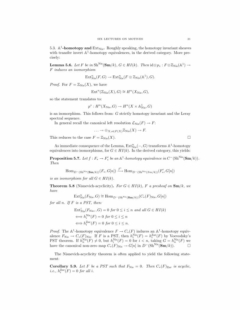
Lemma 5.6. Let F be in ShNis(Sm/k), G ∈ HI(k). Then id⊗p∗ : F⊗ZNis(A1)→F induces an isomorphism

ExtnNis(F,G)→ Extn

Nis(F ⊗ ZNis(A1), G).

Proof. For F = ZNis(X), we have

Extn(ZNis(X), G) ∼= Hn(XNis, G),

so the statement translates to:

p∗ : Hn(XNis, G)→ Hn(X × A1Nis, G)

is an isomorphism. This follows from: G strictly homotopy invariant and the Lerayspectral sequence.

In general recall the canonical left resolution LNis(F )→ F :

. . .→ ⊕X,s∈F (X)ZNis(X)→ F.

This reduces to the case F = ZNis(X).

As immediate consequence of the Lemma, ExtnNis(−, G) transforms A1-homotopy

equivalences into isomorphisms, for G ∈ HI(k). In the derived category, this yields:

Proposition 5.7. Let f : F∗ → F ′∗ be an A1-homotopy equivalence in C−(ShNis(Sm/k)).Then

HomD−(ShNis(Sm/k))(F∗, G[n])f∗−→ HomD−(ShNis(Sm/k))(F

′∗, G[n])

is an isomorphism for all G ∈ HI(k).

Theorem 5.8 (Nisnevich-acyclicity). For G ∈ HI(k), F a presheaf on Sm/k, wehave

ExtnNis(FNis, G) ∼= HomD−(ShNis(Sm/k))(C∗(F )Nis, G[n])

for all n. If F is a PST, then:

ExtiNis(FNis, , G) = 0 for 0 ≤ i ≤ n and all G ∈ HI(k)

⇐⇒ hNisi (F ) = 0 for 0 ≤ i ≤ n

⇐⇒ hZari (F ) = 0 for 0 ≤ i ≤ n.

Proof. The A1-homotopy equivalence F → C∗(F ) induces an A1-homotopy equiv-alence FNis → C∗(F )Nis. If F is a PST, then hNis

i (F ) = hZari (F ) by Voevodsky’s

PST theorem. If hNisn (F ) 6= 0, but hNis

i (F ) = 0 for i < n, taking G = hNisn (F ) we

have the canonical non-zero map C∗(F )Nis → G[n] in D−(ShNis(Sm/k)).

The Nisnevich-acyclicity theorem is often applied to yield the following state-ment:

Corollary 5.9. Let F be a PST such that FNis = 0. Then C∗(F )Zar is acyclic,i.e., hZar

i (F ) = 0 for all i.

22 MARC LEVINE

5.4. The tensor structure. We define a tensor structure on ShNis(Cor(k)):

Set L(X) ⊗ L(Y ) := L(X × Y ). For a general F , we have the canonical leftresolution L(F )→ F :

. . .→ ⊕X,s∈F (X)ZNis(X)→ F

DefineF ⊗G := HNis

0 (L(F )⊗ L(G)).The unit for ⊗ is L(Spec k).

5.5. The localization theorem. We can now prove the main result describingDM eff

− (k) as a localization of D−(ShNis(Cor(k))).

Theorem 5.10. The functor C∗ extends to an exact functor

RC∗ : D−(ShNis(Cor(k)))→ DM eff− (k),

left adjoint to the inclusion DM eff− (k)→ D−(ShNis(Cor(k))). RC∗ identifies DM eff

− (k)with the localization D−(ShNis(Cor(k)))/A, where A is the localizing subcategory ofD−(ShNis(Cor(k))) generated by complexes

L(X × A1)L(p1)−−−→ L(X); X ∈ Sm/k.

Proof. It suffices to prove:

1. For each F ∈ ShNis(Cor(k)), F → C∗(F ) is an isomorphism in D−(ShNis(Cor(k)))/A.2. For each T ∈ DM eff

− (k), B ∈ A, Hom(B, T ) = 0.

Indeed: (1) implies DM eff− (k) → D−(ShNis(Cor(k)))/A is surjective on isomor-

phism classes. (2) implies DM eff− (k) → D−(ShNis(Cor(k)))/A is fully faithful,

hence an equivalence. (1) again implies the composition

D−(ShNis(Cor(k)))→ D−(ShNis(Cor(k)))/A → DM eff− (k)

sends F to C∗(F ).To prove (2): For each T ∈ DM eff

− (k), B ∈ A, Hom(B, T ) = 0. A is generated

by complexes I(X) := L(X × A1)L(p1)−−−→ L(X). But Hom(L(Y ), T ) ∼= H0(YNis, T )

for T ∈ D−(ShNis(Cor(k))) and

H∗(X, T ) ∼= H∗(X × A1, T )

since T is in DM eff− (k), so Hom(I(X), T ) = 0.

To prove (1): For each F ∈ ShNis(Cor(k)), F → C∗(F ) is an isomorphism inD−(ShNis(Cor(k)))/A. Note thatA is a⊗-ideal: A ∈ A, B ∈ D−(ShNis(Cor(k))) =⇒A ⊗ B ∈ A. A is localizing, so can take A = I(X), B = L(Y ). But thenA⊗B = I(X × Y ).

Next, F∗ → C∗(F ) is a term-wise A1-homotopy equivalence and F → F∗ isan iso in D−(ShNis(Cor(k))), so it suffices to show: For each F ∈ ShNis(Cor(k)),id⊗ i0 = id⊗ i1 : F → F ⊗ A1 in D−(ShNis(Cor(k)))/A.

For this, i0 − i1 : L(Spec k)→ L(A1) goes to 0 after composition with L(A1)→L(Spec k), so this map lifts to a map φ : L(Spec k)→ I(A1). Thus id⊗ i0− id⊗ i1 :F → F ⊗ L(A1) lifts to id⊗ φ : F → F ⊗ I(A1) ∈ A.


6. The embedding theorem

We will use the sheaf-theoretic constructions to study the geometric categoryDM eff

gm(k). This relies on constructing a full embedding DM effgm(k)→ DM eff

− (k).Start with the functor

L : Cor(k)→ ShNis(Cor(k))

sending X to the representable sheaf L(X). L extends to the homotopy categoryof bounded complexes:

L : Kb(Cor(k))→ D−(ShNis(Cor(k))).

Theorem 6.1. There is a commutative diagram of exact tensor functors

Kb(Cor(k)) L //

D−(ShNis(Cor(k)))

RC∗

DM effgm(k)

i// DM eff

− (k)

such that

1. i is a full embedding with dense image.2. RC∗(L(X)) ∼= C∗(X).

Corollary 6.2. For X and Y ∈ Sm/k, HomDMeffgm(k)(Mgm(Y ),Mgm(X)[n]) ∼=

Hn(YNis, C∗(X)) ∼= Hn(YZar, C∗(X)).

Proof of the embedding theorem. We already know that RC∗(L(X)) ∼= C∗(L(X)) =C∗(X). To show that i : DM eff

gm(k)→ DM eff− (k) exists:

DM eff− (k) is already pseudo-abelian. Using the localization theorem, we need to

show that the two types of complexes we inverted in Kb(Cor(k)) are already in-verted in D−(ShNis(Cor(k)))/A.

Type hom. [X×A1]→ [X]. This goes to L(X×A1)→ L(X), which is a generatorin A.

Type MV . ([U ∩ V ]→ [U ]⊕ [V ])→ [U ∪ V ]. The sequence

0→ L(U ∩ V )→ L(U)⊕ L(V )→ L(U ∪ V )→ 0

is exact as Nisnevich sheaves, hence the map is inverted in D−(ShNis(Cor(k))).To show that i is a full embedding: Replace D−(ShNis(Cor(k))) with derived

presheaf category D−(PreSh(Cor(k))). Then

L : Kb(Cor(k))→ D−(PreSh(Cor(k)))

is a full embedding, because L(X) is projective in PreSh(Cor(k)).To pass from presheaves to sheaves, note that

D−(PreSh(Cor(k)))→ D−(ShNis(Cor(k)))

is the localization with respect to the localizing category of F such that FNis∼= 0.

Let T be the localizing subcategory of D−(PreSh(Cor(k))) generated by apply-ing L to Type hom and Type MV . It follows from results of Ne’eman on compact

24 MARC LEVINE

objects in triangulated categories that L−1(T ) is the thick subcategory generatedby cones of maps of Type hom and Type MV , so we need to show that, if FNis

∼= 0,then F is in T .

Let Hi : Sm/k → Ab be the functor

Hi(X) := HomD−(PreShNis(Cor(k)))/T (L(X), F [i]).

It suffices to show that all Hi = 0, since the L(X) generate.Since T contains Type MV sequences, Hi give long exact Mayer-Vietoris

sequences, so it suffices to show that HiZar = 0. Since the Hi are PST’s and are

homotopy invariant (Type hom), we have HiZar = Hi

Nis. So we need to show thatHi

Nis = 0.We have already seen that C∗(T )Nis

∼= 0 and K → C∗(K) has cone in T .Represent a morphism φ : L(X)→ F [i] by

L(X)

f""EE

EEEE

EEF [i]

g||

||||

||

K

with Cone(g) ∈ T . By our comments above, we may replace K with C∗(K). ButFNis

∼= 0 =⇒ C∗(F )Nis∼= 0. Also C∗(K)Nis

∼= C∗(F )Nis[i] ∼= 0, so there is aNisnevich cover U → X with composition

L(U)→ L(X)→ K → C∗(K)

being zero. Thus φ goes to 0 in Hi(U).To show that i has dense image: This uses the canonical left resolution L(F )→ F

to show that every object is expressible in terms of direct sums of representableobjects.

6.1. Suslin homology. One can use the Suslin complex to define a purely alge-braic version of singular homology. In fact, this was Suslin’s original construction,which was later generalized to the setting of sheaves with transfers.

Definition 6.3. For X ∈ Sm/k, define the Suslin homology of X as

HSusi (X) := Hi(C∗(X)(Spec k)).

Theorem 6.4. For X ∈ Sm/k, there is a canonical isomorphism

HSusi (X) ∼= HomDMeff

gm(k)(Z[i],Mgm(X)).

Proof. Here Z := Mgm(Spec k). This follows directly from the embedding theorem.

Corollary 6.5. Let U, V be open subschemes of X ∈ Sm/k. Then there is a longexact Mayer-Vietoris sequence

. . .→ HSusn+1(U ∪ V )→ HSus

n (U ∩ V )

→ HSusn (U)⊕HSus

n (V )→ HSusn (U ∪ V )→ . . .

Proof. By the previous theorem, we have

HSusn (Y ) = HomDMeff

− (k)(Z[n],Mgm(Y )).


for all Y ∈ Sm/k, n ∈ Z. Also,

Mgm(U ∩ V )→Mgm(U)⊕Mgm(V )→Mgm(U ∪ V )

extends to a distinguished triangle in DM eff− (k), so the result follows by applying

HomDMeffgm(k)(Z,−) to this distinguished triangle.

26 MARC LEVINE

Lecture 2. Motives and cycle complexes

In this second lecture, we examine the category DM effgm(k) in more detail. The

basic structures we expect from cohomology will all be reflected in structures in thecategory DM eff

gm(k); the examination of these structures will occupy the first partof the lecture. The second part is concerned with giving in some sense a computionof the cohomology theory arising from the category DM eff

gm(k). The computationis acheived through the use of various cycle complexes, which we describe in thesecond half; the proofs of some of the basic results on cycle complexes will be putoff until Lecture 4. The cycle complexes and their properties are used to prove thecancellation theorem: that DM eff

gm(k) → DMgm(k) is an embedding. We concludewith a discusion of duality in DMgm(k).

The material in this lecture is taken mainly from [48].

7. Basic structures in DM effgm(k)

We discuss motivic cohomology, the projective bundle formula and the Gysinisomorphism, realizing these as morphisms and isomorphisms in DM eff

gm.

7.1. Motivic cohomology. We have already seen Suslin homology as

HSusi (X) := Hi(C∗(X)(Spec k)) ∼= HomDMeff

gm(k)(Z[i],Mgm(X)).

The twisted contravariant version is motivic cohomology:

Definition 7.1. For X ∈ Sm/k, q ≥ 0, set

Hp(X, Z(q)) := HomDMeffgm(k)(Mgm(X), Z(q)[p]).

Motivic cohomology has products: Define the cup product

Hp(X, Z(q))⊗Hp′(X, Z(q′))→ Hp+p′(X, Z(q + q′))

by sending a⊗ b to

Mgm(X) δ−→Mgm(X)⊗Mgm(X) a⊗b−−→ Z(p)[q]⊗ Z(p′)[q′] ∼= Z(p + p′)[q + q′].

This makes ⊕p,qHp(X, Z(q)) a graded commutative ring with unit 1 the map

Mgm(X)→ Z induced by pX : X → Spec k.

7.2. Homotopy and Mayer-Vietoris. Applying HomDMgm(−, Z(q)[p]) to theisomorphismp∗ : Mgm(X × A1)→Mgm(X) gives the homotopy property for H∗(−, Z(∗)):

p∗ : Hp(X, Z(q)) ∼−→ Hp(X × A1, Z(q)).

For U, V ⊂ X open subschemes, applying HomDMgm(−, Z(q)[p]) to the distin-guished triangle

Mgm(U ∩ V )→Mgm(U)⊕Mgm(V )→Mgm(U ∪ V )→Mgm(U ∩ V )[1]

gives the Mayer-Vietoris exact sequence for H∗(−, Z(∗)):

. . .→ Hp−1(U ∪ V, Z(q))→ Hp(U ∩ V, Z(q))

→ Hp(U, Z(q))⊕Hp(V, Z(q))→ Hp(U ∪ V, Z(q))→ . . .


7.3. Weight one motivic cohomology. The motivic cohomology in weight 1,H∗(−, Z(1) recovers some well-known invariants.

Z(1)[2] is the reduced motive of P1, and Mgm(P1) is represented in DM eff− by the

Suslin complex C∗(P1). The homology sheaves of C∗(P1) and C∗(Spec k) are givenby:

Lemma 7.2. hZar0 (P1) = Z, hZar

1 (P1) = Gm and hZarn (P1) = 0 for n ≥ 2.

hZar0 (Spec k) = Z, hZar

n (Spec k) = 0 for n ≥ 1.

For Spec k, this is an easy computation, we will prove this for P1 later.This computation implies that Z(1) ∼= Gm[−1] in DM eff

− (k). Indeed:

Z(1)[2] ∼= Cone(C∗(P1)→ C∗(Spec k))[−1] ∼= hZar1 (P1)[1] = Gm[1]

This yields:

Proposition 7.3. For X ∈ Sm/k, we have

Hn(X, Z(1)) =

H0

Zar(X,O∗X) for n = 1Pic(X) := H1

Zar(X,O∗X) for n = 20 else.

Proof. Since Z(1) ∼= Gm[−1] in DM eff− (k), the embedding theorem of Lecture 1

gives:

HomDMeffgm

(Mgm(X), Z(1)[n]) ∼= HnNis(X, Z(1))

∼= HnZar(X, Z(1)) ∼= Hn−1

Zar (X, Gm).

7.4. Chern classes of line bundles.

Definition 7.4. Let L → X be a line bundle on X ∈ Smk. We let c1(L) ∈H2(X, Z(1)) be the element corresponding to [L] ∈ H1

Zar(X,O∗X).

7.5. Projective bundle formula. Let E → X be a rank n + 1 vector bundleover X ∈ Sm/k, q : P(E) → X the resulting Pn−1 bundle, O(1) the tautologicalquotient bundle.

Define αj : Mgm(P(E))→Mgm(X)(j)[2j] by

Mgm(P(E)) δ−→Mgm(P(E))⊗Mgm(P(E))q⊗c1(O(1))j

−−−−−−−−→Mgm(X)(j)[2j]

Theorem 7.5 (Projective bundle formula). The map

αE := ⊕nj=0αj : Mgm(P(E))→ ⊕n

j=0Mgm(X)(j)[2j]

is an isomorphism.

The proof of the projective bundle formula requires the following computation:

Lemma 7.6. There is a canonical isomorphism

Mgm(An \ 0)→ Z(n)[2n− 1]⊕ Z.

Proof. For n = 1, we have Mgm(P1) = Z ⊕ Z(1)[2], by definition of Z(1). TheMayer-Vietoris distinguished triangle

Mgm(A1 \ 0)→Mgm(A1)⊕Mgm(A1)→Mgm(P1)→Mgm(A1 \ 0)[1]

28 MARC LEVINE

defines an isomorphism t : Mgm(A1 \ 0)→ Z(1)[1]⊕ Z.For general n, write An \ 0 = An \An−1 ∪An \A1. By induction, Mayer-Vietoris

and homotopy invariance, this gives the distinguished triangle

(Z(1)[1]⊕ Z)⊗ (Z(n− 1)[2n− 3]⊕ Z)

→ (Z(1)[1]⊕ Z)⊕ (Z(n− 1)[2n− 3]⊕ Z)→Mgm(An \ 0)

→ (Z(1)[1]⊕ Z)⊗ (Z(n− 1)[2n− 3]⊕ Z)[1]

yielding the result.

Proof of the projective bundle formula. The map αE is natural in X, E. Mayer-Vietoris reduces to the case of a trivial bundle, then to the case X = Spec k, so weneed to prove:

Lemma 7.7. ⊕nj=0αj : Mgm(Pn)→ ⊕n

j=0Z(j)[2j] is an isomorphism.

Proof. Write Pn = An ∪ (Pn \ 0). Mgm(An) = Z. Pn \ 0 is an A1 bundle over Pn−1,so induction gives

Mgm(Pn \ 0) = ⊕n−1j=0 Z(j)[2j].

By our computation, we have Mgm(An \ 0) = Z(n)[2n− 1]⊕ Z.The Mayer-Vietoris distinguished triangle

Mgm(An \ 0)→Mgm(An)⊕Mgm(Pn \ 0)→Mgm(Pn)→Mgm(An \ 0)[1]

gives the result.

7.6. The Gysin isomorphism.

Definition 7.8. For i : Z → X a closed embedding in Sm/k, let Mgm(X/X \Z) ∈DM eff

gm(k) be the image in DM effgm(k) of the complex [X \ Z]

j−→ [X], with [X] indegree 0.

Remark 7.9. The Mayer-Vietoris property for Mgm(−) yields a Zariski excisionproperty: If Z is closed in U , an open in X, then Mgm(U/U \ Z)→Mgm(X/ \ Z)is an isomorphism.

In fact, Voevodsky’s moving lemma shows that Mgm(X/X \Z) depends only onthe Nisnevich neighborhood of Z in X: this is the Nisnevic excision property.

Theorem 7.10 (Gysin isomorphism). Let i : Z → X be a closed embedding inSm/k of codimension n. Then there is a natural isomorphism in DM eff

gm(k)

Mgm(X/X \ Z) ∼= Mgm(Z)(n)[2n].

We first prove

Lemma 7.11. Let E → Z be a vector bundle of rank n with zero section s. ThenMgm(E/E \ s(Z)) ∼= Mgm(Z)(n)[2n].

Proof. Since Mgm(E)→Mgm(Z) is an isomorphism by homotopy, we need to show

Mgm(E \ s(Z)) ∼= Mgm(Z)⊕Mgm(Z)(n)[2n− 1].

Let P := P(E ⊕ OZ), and write P = E ∪ (P \ s(Z)). Mayer-Vietoris gives thedistinguished triangle

Mgm(E \ s(Z))→Mgm(E)⊕Mgm(P \ s(Z))→Mgm(P)→Mgm(E \ s(Z))[1]


Since P \ s(Z) → P(E) is an A1 bundle, the projective bundle formula gives theisomorphism we wanted.

The general case uses the deformation to the normal bundle to reduce to thecase of the zero-section of a vector bundle.

7.7. Deformation to the normal bundle. For i : Z → X a closed immersion inSm/k, let p : (X × A1)Z×0 be the blow-up. Set

Def(i) := (X × A1)Z×0 \ p−1[X × 0].

We have i : Z × A1 → Def(i), q : Def(i)→ A1.The fiber i1 is i : Z → X, the fiber i0 is s : Z → NZ/X .

Lemma 7.12. The maps

Mgm(NZ/X/(NZ/X \ s(Z)))→Mgm(Def(i) \ Z × A1)←Mgm(X/(X \ Z))

are isomorphisms.

Proof. By Nisnevich excision, we reduce to the case Z × 0→ Z ×Ad. In this case,Z × A1 → Def(i) is just (Z × 0→ Z × Ad)× A1, whence the result.

The proof of the Gysin isomorphism theorem is now immediate from the twolemmas:

Mgm(X/(X \ Z)) ∼= Mgm(NZ/X/(NZ/X \ s(Z))) ∼= Mgm(Z)(n)[2n]

7.8. Gysin distinguished triangle.

Theorem 7.13. Let i : Z → X be a codimension n closed immersion in Sm/kwith open complement j : U → X. There is a canonical distinguished triangle inDM eff

gm(k):

Mgm(U)j∗−→Mgm(X)→Mgm(Z)(n)[2n]→Mgm(U)[1]

Proof. By definition of Mgm(X/U), we have the canonical distinguished triangle inDM eff

gm(k):

Mgm(U)j∗−→Mgm(X)→Mgm(X/U)→Mgm(U)[1]

then insert the Gysin isomorphism Mgm(X/U) ∼= Mgm(Z)(n)[2n].

Applying HomDMgm(−, Z(q)[p]) to the Gysin distinguished triangle yields thelong exact Gysin sequence for motivic cohomology:

. . .→ Hp−1(U, Z(q)) ∂−→ Hp−2n(Z, Z(q − n))i∗−→ Hp(X, Z(q))

j∗−→ Hp(U, Z(q))→ . . .

8. Cycle complexes and bivariant cycle cohomology

We introduce various cycle complexes and describe their main properties. Wewill discuss the proofs of these in detail in Lecture 4. Our ultimate goal is todescribe the morphisms in DM eff

gm(k) using algebraic cycles, more precisely, as thehomology of a cycle complex.

30 MARC LEVINE

8.1. Bloch’s cycle complex. This is historically the first cycle complex that aroseas a candidate for motivic cohomology, constructed by Bloch in [8]

A face of ∆n := Spec k[t0, . . . , tn]/∑

i ti − 1 is a closed subset defined by ti1 =. . . = tis

= 0.

Definition 8.1. Take X ∈ Schk. zr(X, n) ⊂ zr+n(X × ∆n) is the subgroupgenerated by the closed irreducible W ⊂ X ×∆n such that

dim W ∩X × F ≤ r + dim F

for all faces F ⊂ ∆n.If X is equi-dimensional over k of dimension d, set

zq(X, n) := zd−q(X, n).

Let δni : ∆n → ∆n+1 be the inclusion to the face ti = 0. The cycle pull-back δn∗

i

is a well-defined mapδn∗i : zr(X, n + 1)→ zr(X, n)

Definition 8.2. Bloch’s cycle complex zr(X, ∗) is zr(X, n) in degree n, with dif-ferential

dn :=n+1∑i=0

(−1)iδn∗i : zr(X, n + 1)→ zr(X, n)

Bloch’s higher Chow groups are

CHr(X, n) := Hn(zr(X, ∗)).

For X locally equi-dimensional over k, we have the complex zq(X, ∗) and the higherChow groups CHq(X, n).

Remark 8.3. A problem with functoriality: Even for X ∈ Sm/k, the complexzq(X, ∗) is only functorial for flat maps, and covariantly functorial for proper maps(with a shift in q). This complex is NOT a complex of PST’s.

We will see later that this is corrected in the derived category by a version ofChow’s moving lemma.

8.2. Properties of the higher Chow groups.(0) ProductsThere is an external product zq(X, ∗)⊗zq′(Y, ∗)→ zq+q′(X×k Y, ∗) (in the derivedcategory), induced by taking products of cycles. For X smooth, this induces a cupproduct, using δ∗X .

(1) Homotopyp∗ : zr(X, ∗)→ zr+1(X × A1, ∗) is a quasi-isomorphism for X ∈ Schk.

(2)Localization amd Mayer-VietorisFor X ∈ Schk, let i : W → X be a closed subset with complement j : U → X.Then

zr(W, ∗) i∗−→ zr(X, ∗) j∗−→ zr(U, ∗)canonically extends to a distinguished triangle in D−(Ab). Similarly, if X = U∪V ,U, V open in X, the sequence

zr(X, ∗)→ zr(U, ∗)⊕ zr(V, ∗)→ zr(U ∩ V, ∗)


canonically extends to a distinguished triangle in D−(Ab).

(3) K-theoryFor X regular, there is a functorial Chern character isomorphism

ch : ⊕qCHq(X, n)Q → Kn(X)Q

sending CHq(X, n)Q isomorphically onto the weight q eigenspace Kn(X)(q) for theAdams operations.

(4) Classical Chow groupsCHn(X, 0) = CHn(X) := zn(X)/ rational equivalence.

(5) Weight oneFor X ∈ Sm/k, CH1(X, 1) = H0(X,O∗X), CH1(X, 0) = H1(X,O∗X) = Pic(X),CH1(X, n) = 0 for n > 1.

(6) Chern classes of line bundlesUsing (4) or (5), we have c1(L) ∈ CH1(X, 0) for each line bundle L→ X.

(7) Projective bundle formulaLet E → X be a vector bundle of rank n + 1, q : P(E) → X the Pn bundleof E, ξ := c1(O(1)). Then CH∗(P(E), ∗) is a free CH∗(X, ∗) module with basis1, ξ, . . . , ξn.

The proofs of the functoriality and localization properties use two different typesof moving lemmas, to be discussed in Lecture 4.

8.3. Equi-dimensional cycles. The use of equi-dimensional cycles allows us toform a cycle complex which is a complex of PSTs.

Definition 8.4. Fix X ∈ Schk. For U ∈ Sm/k let zequir (X)(U) ⊂ z(X × U) be

the subgroup generated by the closed irreducible W ⊂ X ×U such that W → U isequi-dimensional with fibers of dimension r (or empty).

Remark 8.5. The standard formula for composition of correspondences makes zequir (X)

a PST; in fact zequir (X) is a Nisnevich sheaf with transfers.

Definition 8.6. The complex of equi-dimensional cycles is

zequir (X, ∗) := C∗(zequi

r (X))(Spec k).

Explicitly: zequir (X, n) is the subgroup of zr+n(X×∆n) generated by irreducible

W such that W → ∆n is equi-dimensional with fiber dimension r. Thus:There is a natural inclusion

zequir (X, ∗)→ zr(X, ∗).

8.4. Bivariant cycle cohomology and the cdh topology. The equivariant cyclecomplexes form the basis for a reasonable cohomology theory on Sm/k. This isformed by combining the Suslin complex construction with hypercohomology in anew Grothendieck topology: the cdh topology.

32 MARC LEVINE

Definition 8.7. The cdh site is given by the pre-topology on Schk with coveringfamilies generated by

1. Nisnevich covers

2. Maps of the form p q i : Y q F → X, where i : F → X is a closed immer-sion, p : Y → X is proper, and p : Y \ p−1F → X \ F is an isomorphism (the mapp is called an abstract blow-up).

Remark 8.8. If k admits resolution of singularities (for finite type k-schemes and forabstract blow-ups to smooth k-schemes), then each cdh cover admits a refinementconsisting of smooth k-schemes.

Definition 8.9. Take X, Y ∈ Schk. The bivariant cycle cohomology of Y withcoefficients in cycles on X are

Ar,i(Y,X) := H−i(Ycdh, C∗(zequir (X))cdh).

Ar,i(Y, X) is contravariant in Y for arbitrary maps, and covariant in X for propermaps. We have the natural map

hi(zequir (X))(Y ) := Hi(C∗(zequi

r (X))(Y ))→ Ar,i(Y, X).

8.5. Mayer-Vietoris and blow-up sequences. Since Zariski open covers andabstract blow-ups are covering families in the cdh topology, we have a Mayer-Vietoris sequence for U, V ⊂ Y :

. . .→ Ar,i(U ∪ V,X)→ Ar,i(U,X)⊕Ar,i(V,X)

→ Ar,i(U ∩ V,X)→ Ar,i−1(U ∪ V,X)→ . . .

and for pq i : Y ′ q F → Y :

. . .→ Ar,i(Y,X)→ Ar,i(Y ′, X)⊕Ar,i(F,X)

→ Ar,i(p−1(F ), X)→ Ar,i−1(Y, X)→ . . .

Additional properties of Ar,i require some fundamental results on the behaviorof homotopy invariant PST’s with respect to cdh-sheafification. Additionally, wewill need some purely geometric results comparing different cycle complexes. Thesetwo types of results are:

1. Acyclicity theorems. We have already seen the Nisnevich acyclicity theorem,one version of which states that for a homotopy invariant PST F with FNis = 0,the Suslin complex C∗(F )Zar is acyclic.

We will also need the cdh version: Assume that k admits resolution of singularities.For F a homotopy invariant PST with Fcdh = 0, the Suslin complex C∗(F )Zar isacyclic.

These two results transform sequences of homotopy invariant PST’s which be-come short exact after cdh-sheafification, into distinguished triangles after applyingC∗(−)Zar.


Using a hypercovering argument, they also show that cdh, Nis and Zar cohomol-ogy of a homotopy invariant PST all agree on smooth varieties.

We will prove the cdh acyclicity theorem and derive its important consequenceslater on in this lecture (see theorem 9.4). The second type of result we need is

2. Moving lemmas. The bivariant cohomology Ar,i is defined using cdh-hyper-cohomology of zequi

r , so comparing zequir with other complexes, such as Bloch’s cycle

complex, leads to identification of Ar,i with cdh-hypercohomology of the other com-plexes. The comparision of zequi

r with other complexes is based partly on geometricconstructions. These moving lemmas will be discussed in Lecture 4.

8.6. Homotopy. Bivariant cycle homolopy is homotopy invariant:

Proposition 8.10. Suppose k admits resolution of singularities. Then the pull-back map

p∗ : Ar,i(Y, X)→ Ar,i(Y × A1, X)

is an isomorphism.

Proof. Using hypercovers and resolution of singularities, we reduce to the caseof smooth Y . As mentioned above, the cdh-acyclicity theorem changes the cdhhypercohomology defining Ar,i to Nisnevich hypercohomology. Since the homologypresheaves of C∗(zequi

r (X)) are homotopy invariant PST’s, we can use Voevodsky’sPST theorem to conclude the homotopy invariance.

8.7. The geometric comparison theorem.

Theorem 8.11 (Geometric comparison). Suppose k admits resolution of singular-ities. Take X ∈ Schk. Then the natural map zequi(X, ∗) → zr(X, ∗) is a quasi-isomorphism.

(2) For U smooth and quasi-projective, the natural map

hi(zequir (X))(U)→ Ar,i(U,X)

is an isomorphism.

The proof of this result is based on Suslin’s moving lemma. We will discuss thedetails of the proof in Lecture 4.

8.8. The geometric duality theorem. Let zequir (Z,X) := Hom(L(Z), zequi

r (X)).Explicitly:

zequir (Z,X)(U) = zequi

r (X)(Z × U).

We have the inclusion zequir (Z,X)→ zequi

r+dim Z(X × Z).

Theorem 8.12 (Geometric duality). Suppose k admits resolution of singularities.Take X ∈ Schk, U ∈ Sm/k, quasi-projective of dimension n. Then the inclusionzequir (U,X)→ zequi

r+n(X×U) induces a quasi-isomorphism of complexes on Sm/kZar:

C∗(zequir (U,X))Zar → C∗(z

equir+n(X × U))Zar

The proof for U and X smooth and projective uses the Friedlander-Lawsonmoving lemma. The extension to U smooth quasi-projective, and X general usesthe cdh-acyclicity theorem. We will discuss the details of the proof in Lecture 4.

34 MARC LEVINE

8.9. The cdh comparison and duality theorems.

Theorem 8.13 (cdh comparison). Suppose k admits resolution of singularities.Take X ∈ Schk. Then for U smooth and quasi-projective, the natural map

hi(zequir (X))(U)→ Ar,i(U,X)

is an isomorphism.

Theorem 8.14 (cdh duality). Suppose k admits resolution of singularities. TakeX, Y ∈ Schk, U ∈ Sm/k of dimension n. There is a canonical isomorphism

Ar,i(Y × U,X)→ Ar+n,i(Y, X × U).

To prove the cdh comparison theorem, first use the cdh-acyclicity theorem toidentify

H−iZar(U, zequi

r (X)) ∼−→ H−icdh(U, zequi

r (X)) =: Ar,i(U,X)Next, if V1, V2 are Zariski open in U , use the geometric duality theorem to identifythe Mayer-Vietoris sequence

C∗(zequir (X))(V1 ∪ V2)→ C∗(zequi

r (X))(V1)⊕ C∗(zequir (X))(V2)

→ C∗(zequir (X))(V1 ∩ V2)

with

0→ C∗(zequir (X × (V1 ∪ V2))→ C∗(zequi

r (X × V1))⊕ C∗(zequir (X × V2))

→ C∗(zequir (X × (V1 ∩ V2))

evaluated at Spec k.But this presheaf sequence is exact, and cokercdh = 0. The cdh-acyclicity theo-

rem thus gives us the distinguished triangle

C∗(zequir (X × (V1 ∪ V2))Zar

→ C∗(zequir (X × V1))Zar ⊕ C∗(zequi

r (X × V2))Zar

→ C∗(zequir (X × (V1 ∩ V2))Zar →

Evaluating at Spec k, we find that our original Mayer-Vietoris sequence for C∗(zequir (X))

was in fact a distinguished triangle.The Mayer-Vietoris property for C∗(zequi

r (X)) formally implies that

hi(C∗(zequir (X)))(U)→ H−i

Zar(U,C∗(zequir (X)))

is an isomorphism.

To prove the cdh-duality theorem,

Ar,i(Y × U,X) ∼= Ar+n,i(Y,X × U).

write U = ∪iUi as a union of quasi-projective open subschemes, and let zequir (U , X)

be the Cech complex formed from the zequir (Ui, X).

The duality quasi-iso’s zequir (Ui, X) → zequi

r (X × Ui) and a cdh-acyclicity argu-ment as in the proof of the comparison theorem give the quasi-iso

C∗(zequir (U , X))cdh → C∗(zequi(X × U))cdh.


Thus, we need only check that the map

H−icdh(Y, C∗(zequi

r (U , X))cdh)→ H−icdh(Y × U,C∗(zequi

r (X))cdh) = Ar,i(Y × U)

is an isomorphism. This assertion is cdh-local on Y , so we can assume Y is smoothand quasi-projective.

In this case, we can pass from cdh-hypercohomology to Zariski hypercohomology,and then reduce to showing

H−iZar(Y, C∗(zequi

r (Ui, X))Zar)→ H−iZar(Y × Ui, C∗(zequi

r (X))Zar)

is an isomorphism. It follows from the geometric comparison and duality theoremsthat both sides are hi(zequi

r (X))(Y × Ui).

8.10. The cdh-descent theorem.

Theorem 8.15 (cdh-descent). Suppose k admits resolution of singularities. TakeY ∈ Schk.(1) Let U ∪ V = X be a Zariski open cover of X ∈ Schk. There is a long exactsequence

. . .→ Ar,i(Y, U ∩ V )→ Ar,i(Y, U)⊕Ar,i(Y, V )

→ Ar,i(Y, X)→ Ar,i−1(Y,U ∩ V )→ . . .

(2) Let Z ⊂ X be a closed subset. There is a long exact sequence

. . .→ Ar,i(Y, Z)→ Ar,i(Y, X)→ Ar,i(Y,X \ Z)→ Ar,i−1(Y, Z)→ . . .

(3) Let pq i : X ′ q F → X be an abstract blow-up. There is a long exact sequence

. . .→ Ar,i(Y, p−1(F ))→ Ar,i(Y, X ′)⊕Ar,i(Y, F )

→ Ar,i(Y, X)→ Ar,i−1(Y, p−1(F ))→ . . .

Proof. For (1) and (3), the analogous properties are obvious in the “first variable”,so the theorem follows from duality.

For (2), the presheaf sequence

0→ zequir (Z)→ zequi

r (X)→ zequir (X \ U)

is exact and cokercdh = 0. The cdh-acyclicity theorem says that applying C∗(−)cdh

to the above sequence yields a distinguished triangle.

Corollary 8.16 (Duality). For X, Y ∈ Schk, n = dim Y we have a canonicalisomorphism

CHr+n(X × Y, i) ∼= Ar,i(Y, X)

Proof. For U ∈ Sm/k, quasi-projective, we have the quasi-isomorphisms

C∗(zequir+n(X × U))(Spec k) = zequi

r+n(X × U, ∗)→ zr+n(X × U, ∗)

C∗(zequir (U,X))(Spec k)→ C∗(z

equir+n(X × U))(Spec k)

and the isomorphisms

Ar,i(U,X)→ Ar+n,i(Spec k, X × U)← hi(zequir+n(X × U))(Spec k)

This gives the isomorphism

CHr+n(X × U, i)→ Ar,i(U,X).

36 MARC LEVINE

One checks this map is natural with respect to the localization sequences forCHr+n(X ×−, i) and Ar,i(−, X).

Given Y ∈ Schk, there is a filtration by closed subsets

∅ = Y−1 ⊂ Y0 ⊂ . . . ⊂ Ym = Y

with Yi \Yi−1 ∈ Sm/k and quasi-projective (k is perfect), so this extends the resultfrom U ∈ Sm/k, quasi-projective, to Y ∈ Schk.

Corollary 8.17. Suppose k admits resolution of singularities. For X, Y ∈ Schk

we have(1) (homotopy)The projection p : X × A1 → X induces an isomorphism p∗ :Ar,i(Y, X)→ Ar+1,i(Y, X × A1).

(2) (suspension) The maps i0 : X → X × P1, p : X × P1 → X induce an iso-morphism

Ar,i(Y,X)⊕Ar−1,i(Y, X)i∗+p∗−−−−→ Ar,i(Y, X × P1)

(3)(cosuspension) There is a canonical isomorphism

Ar,i(Y × P1, X) ∼= Ar,i(Y, X)⊕Ar+1,i(Y,X)

(4) (localization) Let i : Z → U be a codimension n closed embedding in Sm/k.Then there is a long exact sequence

. . .→ Ar+n,i(Z,X)→ Ar,i(U,X)j∗−→ Ar,i(U \ Z,X)→ Ar+n,i−1(Z,X)→ . . .

Proof. These all follow from the corresponding properties of CH∗(−, ∗) and theduality corollary:

(1) from homotopy(2) and (3) from the projective bundle formula(4) from the localization sequence.

9. Motives of schemes of finite type

We can use the cdh-site to define both the motive of a scheme of finite type, aswell as the motive with compact supports. Taking motivic cohomology, this givesa good definition of motivic cohomology and motivic cohomology with compactsupports for an arbitrary finite type k-scheme.

9.1. Motives and motives with compact support. Recall: For X ∈ Schk,L(X) is the PST with L(X)(U) the free abelian group on irreducible W ⊂ U ×Xsuch that W → U is finite, and surjective onto some component of U . We haveC∗(X) := C∗(L(X)).

Definition 9.1. X ∈ Schk, Lc(X) is the PST with Lc(X)(U) the free abeliangroup on irreducible W ⊂ U ×X such that W → U is quasi-finite, and dominantonto some component of U .

We let Cc∗(X) := C∗(Lc(X)).

This gives us functors

C∗ : Schk → DM eff− (k)

Cc∗ : Sch′k → DM eff

− (k)


where Sch′k ⊂ Schk is the subcategory with the same objects as Schk, but withonly the proper morphisms.

Before we study Cc∗, we state and prove the cdh-acyclicity theorem.

9.2. The cdh-acyclicity theorem. There is a fundamental extension of the Nisnevich-acyclicity theorem 5.8, 5.9 to the cdh topology:

Theorem 9.2 (cdh-acyclicity). Suppose that k admits resolution of singularities.Take G ∈ HI(k), F a presheaf on Sm/k. If Fcdh = 0, then for all n

ExtnNis(FNis, G) = 0.

The crucial fact needed for the proof is:

Lemma 9.3. Let i : Z → X be a closed immersion in Sm/k, p : XZ → U theblow-up of X along Z, G ∈ HI(k). Then for all i ≥ 0

ExtiNis(coker(ZNis(XZ)→ ZNis(X)), G) = 0.

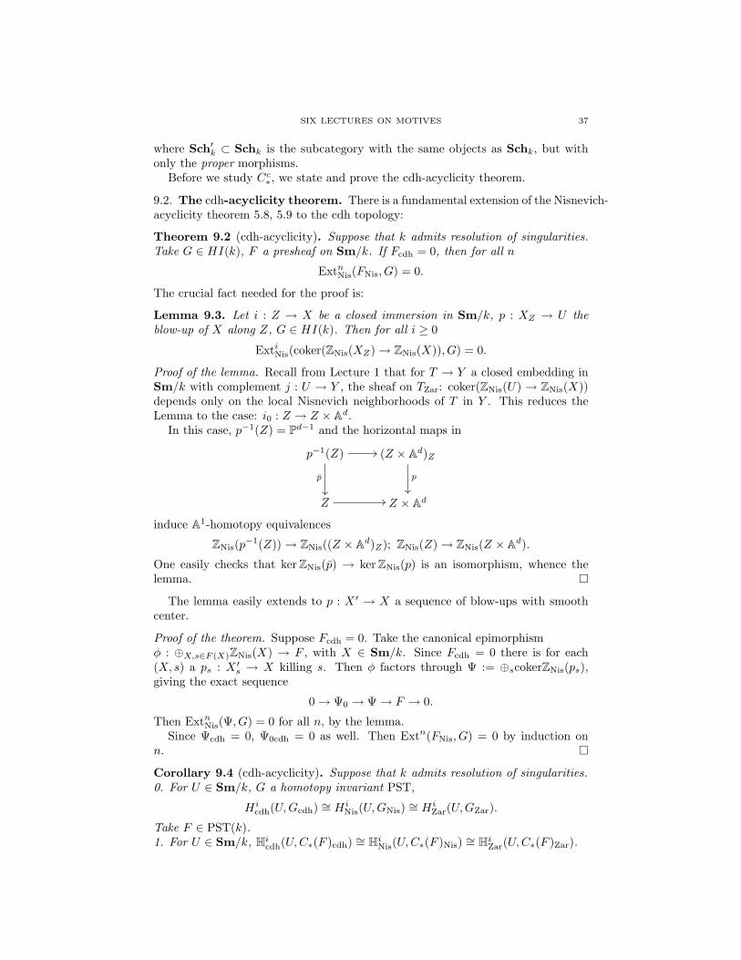
Proof of the lemma. Recall from Lecture 1 that for T → Y a closed embedding inSm/k with complement j : U → Y , the sheaf on TZar: coker(ZNis(U) → ZNis(X))depends only on the local Nisnevich neighborhoods of T in Y . This reduces theLemma to the case: i0 : Z → Z × Ad.

In this case, p−1(Z) = Pd−1 and the horizontal maps in

p−1(Z) //

p

(Z × Ad)Z

p

Z // Z × Ad

induce A1-homotopy equivalences

ZNis(p−1(Z))→ ZNis((Z × Ad)Z); ZNis(Z)→ ZNis(Z × Ad).

One easily checks that ker ZNis(p) → ker ZNis(p) is an isomorphism, whence thelemma.

The lemma easily extends to p : X ′ → X a sequence of blow-ups with smoothcenter.

Proof of the theorem. Suppose Fcdh = 0. Take the canonical epimorphismφ : ⊕X,s∈F (X)ZNis(X) → F , with X ∈ Sm/k. Since Fcdh = 0 there is for each(X, s) a ps : X ′

s → X killing s. Then φ factors through Ψ := ⊕scokerZNis(ps),giving the exact sequence

0→ Ψ0 → Ψ→ F → 0.

Then ExtnNis(Ψ, G) = 0 for all n, by the lemma.

Since Ψcdh = 0, Ψ0cdh = 0 as well. Then Extn(FNis, G) = 0 by induction onn.

Corollary 9.4 (cdh-acyclicity). Suppose that k admits resolution of singularities.0. For U ∈ Sm/k, G a homotopy invariant PST,

Hicdh(U,Gcdh) ∼= Hi

Nis(U,GNis) ∼= HiZar(U,GZar).

Take F ∈ PST(k).1. For U ∈ Sm/k, Hi

cdh(U,C∗(F )cdh) ∼= HiNis(U,C∗(F )Nis) ∼= Hi

Zar(U,C∗(F )Zar).

38 MARC LEVINE

2. If Fcdh = 0, then C∗(F )Zar is acyclic.

3. For X ∈ Schk, p∗ : Hicdh(X, C∗(F )cdh) → Hi

cdh(X × A1, C∗(F )cdh) is an iso-morphism.

4. For X ∈ Schk there are canonical isomorphisms

HomDMeff− (k)(C∗(X), C∗(F )[i]) ∼= Hi

cdh(X, C∗(F )cdh)

Proof. (0) =⇒ (1) since Hi(C∗(F )) is homotopy invariant. For (0), we knowHi

Nis(U,GNis) ∼= HiZar(U,GZar) from Lecture 1.

We go from HiNis(U,GNis) to Hi

cdh(U,GNis) by replacing U with a limit of cdh-hypercovers U . But (coker ZNis(U)→ ZNis(U))cdh = 0, so by the theorem

Hicdh(U,Gcdh) = lim

UHomD(ShNis(Sm/k))(ZNis(U), G[i])

= HomD(ShNis(Sm/k))(ZNis(U), G[i])

= HiNis(U,GNis)

For (2): Suffices to show hNisi (F ) = 0 for all i. If not, there is a non-trivial map

C∗(F )Nis → hNisn (F )[n] in D(ShNis(Sm/k)). But from Lecture 1:

Hom(C∗(F )Nis, hNisn (F )[n]) ∼= Extn

Nis(FNis, hNisn (F ))

which is 0 if Fcdh = 0.(3) and (4) are just like (1): use cdh-hypercovers to reduce from cdh to Nis.

(3) reduces to the homotopy invariance of H∗Nis(−, hi(F )Nis) and (4) reduces to the

isomorphism in the Nisnevic acyclicity theorem 5.8 from Lecture 1:

ExtnNis(L(X), G) ∼= HomD−(ShNis(Sm/k))(C∗(X), G[n])

for G ∈ HI(k).

9.3. Fundamental exact sequences.

Theorem 9.5 (Mayer-Vietoris). Let U ∪ V = X be an open cover of X ∈ Schk.There is a canonical distinguished triangle in DM eff

− (k):

C∗(U ∩ V )→ C∗(U)⊕ C∗(V )→ C∗(X)→ C∗(U ∩ V )[1]

giving a long exact sequence in Suslin homology

. . .→ HSusn+1(X)→ HSus

n (U ∩ V )→ HSusn (U)⊕HSus

n (V )→ HSusn (X)→ . . .

Proof. This uses the Nisnevic-acyclicity theorem 5.9, noting that

0→ L(U ∩ V )→ L(U)⊕ L(V )→ L(X)→ coker → 0

is exact (as presheaves) and cokerNis = 0.

Theorem 9.6 (Blow-up). Suppose k admits resolution of singularities. Let pq i :Y q F → X be an abstract blow-up. There is a canonical distinguished triangle inDM eff

− (k):

C∗(p−1(Z))→ C∗(Y )⊕ C∗(F )→ C∗(X)→ C∗(p−1(F ))[1]


Theorem 9.7 (Localization). Suppose k admits resolution of singularities. Leti : W → X be a closed immersion in Schk with open complement j : U → X.There is a distinguished triangle in DM eff

− (k):

Cc∗(W )→ Cc

∗(X)→ C∗c (U)→ Cc

∗(W )[1]

Proof of the blow-up theorem. The sequence

0→ L(p−1(Z))→ L(Y )⊕ L(Z)→ L(X)→ coker → 0

is exact, with cokercdh = 0. Then apply (2) of the cdh-acyclicity corollary 9.4

The proof of the localization theorem is the same, since

0→ Lc(W )→ Lc(X)→ Lc(U)→ coker → 0

is exact, with cokercdh = 0.

Corollary 9.8. Suppose k admits resolution of singularities. Then both C∗ andCc∗ factor canonically through the embedding i : DM eff

gm(k)→ DM eff− (k).

Proof. For C∗: If Y is in Sm/k, then C∗(Y ) = i(Mgm(Y )). For arbitrary X,C∗(Xred) = C∗(X), so can assume X = Xred. Then use resolution of singularities,induction on dimension and the blow-up distinguished triangle.

For Cc∗: Same as above: k is perfect, so for X ∈ Schk reduced, there is a filtration

by closed subsets∅ = X−1 ⊂ X0 ⊂ . . . ⊂ Xn = X

with Xi \Xi−1 ∈ Sm/k. Then use the localization distinguished triangle.

Definition 9.9. Suppose k admits resolution of singularities. Let

Mgm : Schk → DM effgm(k)

M cgm : Sch′k → DM eff

gm(k)

be the functors with i Mgm = C∗, i M cgm = Cc

∗, as given by the Corollary.Mgm(X) is the motive of X, M c

gm(X) is the motive of X with compact supports.

Remarks 9.10. (1) Suppose X is proper over k. Then Lc(X) = L(X), henceM c

gm(X) = Mgm(X).

(2) M cgm(An) ∼= Z(n)[2n]. This follows from the localization distinguished triangle

Mgm(Pn−1)→Mgm(Pn)→M cgm(An)→Mgm(Pn−1)[1]

and the projective bundle formula.

(3) Changing C∗ to Mgm and Cc∗ to M c

gm, we have Mayer-Vietoris, blow-up andlocalization distinguished triangles in DM eff

gm(k).

10. Morphisms and cycles

We describe how morphisms in DM effgm(k) can be realized as algebraic cycles. This

correspondes to Hanamura’s construction of motives via “higher correspondences”(see [21]). We assume throughout that k admits resolution of singularities.

40 MARC LEVINE

10.1. Bivariant cycle cohomology reappears. The cdh-acyclicity theorem re-lates the bivariant cycle cohomology (and hence higher Chow groups) to the mor-phisms in DM eff

gm(k).

Theorem 10.1. For X, Y ∈ Schk r ≥ 0, i ∈ Z, there is a canonical isomorphism

HomDMeffgm(k)(Mgm(Y )(r)[2r + i],M c

gm(X)) ∼= Ar,i(Y,X).

Proof. For r = 0, the cdh acyclicity theorem 9.4(4) gives an isomorphism

HomDMeff− (k)(C∗(Y )[i], Cc

∗(X)) ∼= H−icdh(Y, C∗(z

equi0 (X))) = A0,i(Y, X).

ThusHomDMeff

− (k)(C∗(Y × (P1)r)[i], Cc∗(X)) ∼= A0,i(Y × (P1)r, X).

By the cosuspension isomorphism (corollary 8.17(3)) Ar,i(Y,X) is a summand ofA0,i(Y × (P1)r, X); by the definition of Z(1), Mgm(Y )(r)[2r] is a summand ofMgm(Y × (P1)r). One checks the two summands match up.

10.2. Chow motives.

Corollary 10.2. Sending a smooth projective variety X of dimension n to Mgm(X)extends to a full embedding M eff

CH(k)→ DM effgm(k), M eff

CH(k) := effective homologicalChow motives.

Proof. For X and Y smooth and projective

HomDMeffgm(k)(Mgm(Y ),Mgm(X)) = A0,0(Y, X)

∼= Adim Y,0(Spec k, Y ×X)∼= CHdim Y (Y ×X)

= HomMeffCH(k)(Y, X).

The cancellation theorem 2.14 thus gives a full embedding

Mgm : MCH(k)→ DMgm(k).

10.3. The Chow ring reappears.

Corollary 10.3. For Y ∈ Schk, equi-dimensional over k, i ≥ 0, j ∈ Z, CHi(Y, j) ∼=HomDMeff

gm(k)(Mgm(Y ), Z(i)[2i− j]). That is

CHi(Y, j) ∼= H2i−j(Y, Z(i)).

Proof. Take i ≥ 0. Then M cgm(Ai) ∼= Z(i)[2i] and

A0,j(Y, Ai) ∼= Adim Y,j(Spec k, Y × Ai)

= CHdim Y (Y × Ai, j)

= CHi(Y × Ai, j)∼= CHi(Y, j)


Remark 10.4. Combining the Chern character isomorphism

ch : CHi(Y, j)Q ∼= Kj(Y )(i)

(for Y ∈ Sm/k) with our isomorphism CHi(Y, j) ∼= H2i−j(Y, Z(i)) identifies ratio-nal motivic cohomology with weight-graded K-theory:

H2i−j(Y, Q(i)) ∼= Kj(Y )(i).

Thus motivic cohomology gives an integral version of weight-graded K-theory, inaccordance with conjectures of Beilinson on mixed motives.

The computation (theorem 10.1) of morphisms in DMeff− (k) as bivariant cycle

cohomology leads to a proof of the cancellation theorem 2.14 and other relatedresults. We recall the statement:

Corollary 10.5 (cancellation). For A,B ∈ DM effgm(k) the map

−⊗ id : Hom(A,B)→ Hom(A(1), B(1))

is an isomorphism. Thus

DM effgm(k)→ DMgm(k)

is a full embedding.

Corollary 10.6. For Y ∈ Schk, n, i ∈ Z, set

Hn(Y, Z(i)) := HomDMgm(k)(Mgm(Y ), Z(i)[n]).

Then Hn(Y, Z(i)) = 0 for i < 0 and for n > 2i.

Corollary 10.7. The full embedding M effCH(k) → DM eff

gm(k) extends to a full em-bedding

Mgm : MCH(k)→ DMgm(k).

Proof of the cancellation theorem and corollaries. The Gysin distinguished trian-gle for for Mgm shows that DM eff

gm(k) is generated by Mgm(X), X smooth andprojective. So, we may assume A = Mgm(Y )[i], B = Mgm(X), X and Y smoothand projective, i ∈ Z.

Then Mgm(X) = M cgm(X) and Mgm(X)(1)[2] = M c

gm(X × A1). Thus:

Hom(Mgm(Y )(1)[i],Mgm(X)(1)) ∼= A1,i(Y, X × A1)∼= A0,i(Y, X)∼= Hom(Mgm(Y )[i],Mgm(X))

For the second corollary, supposes i < 0. Quasi-invertibility implies

H2i−j(Y, Z(i)) = HomDMeffgm(k)(Mgm(Y )(−i)[j − 2i], Z)

= A−i,j(Y,Spec k)

= Adim Y−i,j(Spec k, Y )

= H−j(C∗(zequidim Y−i(Y ))(Spec k)).

Since dim Y − i > dim Y , zequidim Y−i(Y ) = 0.

If i ≥ 0 but n > 2i, then Hn(Y, Z(i)) = CHi(Y, 2i− n) = 0.

42 MARC LEVINE

11. Duality

We describe the duality involution

∗ : DMgm(k)op → DMgm(k),

assuming k admits resolution of singularities.

11.1. Internal Hom. Recall the internal Hom in PST(k) defined in Lecture 1:

Hom(F,G)(U) := Hom(F ⊗ L(U), G)

We have:

Hom(L(X), G)(U) = G(U ×X);

Hom(F,G) := H0Nis(Hom(L(F ), G))

Hom(F,Hom(G, H)) ∼= Hom(F ⊗G, H).

Also if G is a Nisnevich sheaf with transfers (resp. homotopy invariant), then so isHom(F,G).

Now take A,B ∈ C−(ShNis(Cor(k)). We have the internal Hom complexHom(A,B)in C(ShNis(Cor(k)), with

Hom(A⊗B,C) ∼= Hom(A,Hom(B,C)).

This gives the right-derived version RHom(A,B) in D(ShNis(Cor(k)).

Proposition 11.1. If A is in the image of DM effgm(k) and B is in DM eff

− (k), thenRHom(A,B) is in DM eff

− (k).

Proof. For A = C∗(X), the Nisnevic acyclicity theorem 5.8 implies that the coho-mology sheaf Hn(RHom(A,B)) is the sheaf RnpX∗(B) associated to the presheafU 7→ Hn

Zar(U × X, B). Since a homotopy invariant sheaf with transfers is strictlyhomotopy invariant, the Hn(RHom(A,B)) are homotopy invariant. This passes toRHom(A,B) for arbitrary A.

Since RnpX∗(B) is in HI(k), the restriction map

RnpX∗(B)(U)→ RnpX∗(B)(k(U))

is injective for each U ∈ Sm/k, by Voevodsky’s moving lemma.Since Xk(U) has Zariski cohomological dimension dim X and B is bounded above,

RnpX∗(B) = 0 for n >> 0. Thus RHom(A,B) is in D−, hence in DM eff− (k).

In general, RHom(A,B) is not in the image of DM effgm, even if both A and B

are so. Our first task is to show that RHom(A,B)(N) is in DM effgm for N >> 0

(depending on A and B). Write

HomDMeff−

(A,B) := RHom(i(A), i(B))

if A and B are in DM effgm.


11.2. Duality for smooth proper X. Let X be smooth and proper of dimensionn. Then

HomDMeffgm(k)(Mgm(X)⊗Mgm(X), Z(n)[2n]) ∼= CHn(X ×X),

so we have δ : Mgm(X)⊗Mgm(X)→ Z(n)[2n].

Lemma 11.2. For Y smooth and projective, the map

Mgm(X)⊗Mgm(Y )(m) δ∗−→ HomDMeff−

(Mgm(X),Mgm(Y )(n + m)[2n])

induced by δ is an isomorphism for all m ≥ 0

Proof. δ∗ induces

Hom(Mgm(U)[i],Mgm(X × Y )(m))

→ Hom(Mgm(U)[i],HomDMeff−

(Mgm(X),Mgm(Y )(n + m)[2n]))

= Hom(Mgm(U ×X)[i],Mgm(Y )(n + m)[2n])

The LHS is A0,i+2m(U,X × Y × Am), the RHS is

A0,i+2m(U ×X, Y × An+m) ∼= An,i+2m(U,X × Y × An+m)∼= A0,i+2m(U,X × Y × Am).

Since DM effgm(k) is generated by the Mgm(U), this suffices.

Lemma 11.3. Take X, Y smooth and projective with dim X = n. Then for allm ≥ n, the canonical morphism

HomDMeff−

(Mgm(X),Mgm(Y )(n))(m− n)

→ HomDMeff−

(Mgm(X),Mgm(Y )(m))

is an isomorphism.

Proof. Both sides are Mgm(X × Y )(m− n).

Proposition 11.4. Take A,B ∈ DM effgm(k). There is an N = N(A,B) such that

for all m ≥ N :

(1) HomDMeff−

(A,B(m)) is in DM effgm(k).

(2) HomDMeff−

(A,B(m))(a)→ HomDMeff−

(A(n), B(n + m + a)) is an isomorphismfor all a, n ≥ 0.

Proof. For A = Mgm(X), B = Mgm(Y ), X, Y smooth and projective, this fol-lows from the two lemmas and the cancellation theorem. This suffices since thesegenerate DM eff

gm(k).

Definition 11.5. Take A,B ∈ DMgm. Define

HomDMgm(A,B) := HomDMeff−

(A(n), B(n + N))(−N)

where n >> 0 is taken so A(n) and B(n) are in DM effgm(k) and N ≥ N(A(n), B(n)).

It follows from the proposition thatHomDMgm(A,B) is independent of the choiceof n and N .

Set A∗ := HomDMgm(A, Z).

44 MARC LEVINE

Theorem 11.6 (Duality). (1) For A ∈ DMgm(k), the canonical map A → (A∗)∗

is an isomorphism.

(2) For A,B ∈ DMgm(k) there are canonical isomorphisms

(A⊗B)∗ ∼= A∗ ⊗B∗

Hom(A,B) ∼= A∗ ⊗B

(3) For X ∈ Sm/k of dimension n there are canonical isomorphisms

Mgm(X)∗ ∼= M cgm(X)(−n)[−2n]

M cgm(X)∗ ∼= Mgm(X)(−n)[−2n]

Proof. For (1) and (2), we may take A = Mgm(X), B = Mgm(Y ) with X, Y smoothand projective of dimensions n and m. Then we have shown:

Mgm(X)∗ = Mgm(X)(−n)[−2n]

Mgm(X × Y )∗ = Mgm(X × Y )(−n−m)[−2n− 2m]

= Mgm(X)∗ ⊗Mgm(Y )∗

Hom(Mgm(X),Mgm(Y )) = Mgm(X × Y )(−n)[−2n]

= Mgm(X)∗ ⊗Mgm(Y ).

For (3): Let n = dim X. For all U ∈ Sm/k we have canonical isomorphisms

Hom(Mgm(U)[i],HomDMeff−

(Mgm(X), Z(n)[2n]))

= Hom(Mgm(U ×X)[i], Z(n)[2n])

= A0,i(U ×X, An)

= An,i(U,X × An)

= A0,i(U,X)

= Hom(Mgm(U)[i],M cgm(X))

Since the Mgm(U)[i] generate, we have

HomDMeff−

(Mgm(X), Z(n)[2n]) ∼= M cgm(X).


Lecture 3. Mixed Tate motives

The most basic motives are the powers Z(n) of the Tate motive Z(1). The fulltriangulated subcategory DMT(k) of DMgm(k) generated by the “pure” Tate mo-tives Z(n) is the triangulated category of mixed Tate motives over k. Even thoughconcrete computations in the full category DMgm(k) are often very difficult, andmany suspected structural properties rely on (up to now) inaccessible conjectures,the mixed Tate category is much more amenable to such analysis. Especially in thecase of number fields, there is enough known so that DMT(k)Q looks just like a gen-eralization of the classical derived category of sheaves, or perhaps more precisely,like the derived category of the category of representations of an algebraic groupG. In this lecture, we discuss these constructions and give some applications, suchas relating mixed Tate motives with the action of Gal(Q) on πalg

1 (P1 \ 0, 1,∞)and showing that multiple zeta values arise as periods of mixed Tate motives.

12. Mixed Tate motives in DMgm(k)

12.1. Let DMgm(k)Q denote the Q-localization of DMgm(k), i.e. the objects arethe same and

HomDMgm(k)Q(A,B) := HomDMgm(k)(A,B)⊗Q.

We denote the image of the Tate objects Z(n) in DMgm(k)Q by Q(n).

Definition 12.1. The triangulated category DMT(k) of mixed Tate motives overk is the full triangulated subcategory of DMgm(k)Q generated by the Tate motivesQ(n), n ∈ Z. DMTeff(k) is the full triangulated subcategory generated by the Q(n),n ≥ 0.

Here we take “generated” to mean that DMT(k) is the smallest full triangu-lated subcategory of DMgm(k) containing all the objects Q(n) and closed underisomorphism in DMgm(k).

Remark 12.2. DMT(k) is a triangulated tensor subcategory of DMgm(k).

Examples 12.3. (1) Take x ∈ k×. We have the corresponding element

[x] ∈ H1(k, Q(1)) = HomDMgm(k)(Z, Z(1)[1])⊗Q.

Fill in [x] : Z → Z(1)[1] to a distinguished triangle Ex → Z → Z(1)[1] → Ex[1].Then the image of Ex in DMgm(k)Q is in DTM(k).

(2) The same construction gives an element Ex for each x ∈ H1(k, Q(n)).

12.2. t-structures. We are interested in finding an additional structure on DMT(k)Qwhich will give us an abelian category. Following Beilinson-Bernstein-Deligne [6],this is given by a t-structure.

Let A be an abelian category. In D(A), one has full subcategories:

D≤0 := C | Hn(C) = 0 for n > 0,D≥0 := C | Hn(C) = 0 for n < 0.

These satisfy:

1. D≤0[1] ⊂ D≤0, D≥0[−1] ⊂ D≥0.

46 MARC LEVINE

2. Each X ∈ D(A) fits in a distinguished triangle X≤0 → X → X>0 → X≤1[1]with X≤0 ∈ D≤0, X>0 ∈ D>0 := D≥0[−1].

3. Hom(D≤0, D>0) = 0.

Also, sending M ∈ A to the complex M in degree zero gives an equivalance ofA with D≤0 ∩ D≥0; the inverse is given by the cohomology functor H0. Also, asequence in A is exact iff it extends to a distinguished triangle in D(A). Finally, ifA → B → C → A[1] is a distinguished triangle in D(A) with A,C ∈ A, then B isin A (A is closed under extensions in D(A)).

Abstracting these constructions and properties leads to

Definition 12.4 ([6]). (D,D≤0, D≥0) with D a triangulated category and D≤0,

D≥0 satisfying (1)-(3) is a t-structure on D. The full additive subcategory D≤0 ∩D≥0 is the heart of the t-structure.

Theorem 12.5 (Beilinson-Bernstein-Deligne). The heart A of a t-structure on Dis an abelian category, closed under extensions in D, with a sequence in A exact iffthe sequence extends to a distinguished triangle in D.

Remarks 12.6. (1) D is not always a derived category of A!

(2) Set X≤n := (X[n]≤0)[−n], X≥n := (X[1− n]>0)[n− 1]. Sending X to X≤n orX≥n define functors

τ≤n : D → D≤n := D≤0[n],

τ≥n : D → D≥n := D≥0[−n],

right (resp. left) adjoint to the inclusions D≤n → D, D≥n → D. The functorfunctor H0 := τ≤0 τ≥0 : D → A is a cohomological functor, with Hn = τ≤n τ≥n.H0 gives the inverse to the inclusion A → D.

12.3. The weight filtration.

Definition 12.7. W≤nDMT(k) is the full triangulated subcategory of DMT(k)generated by the Tate objects Q(−m) with m ≤ n.

This gives the tower of triangulated subcategories

. . . ⊂W≤nDMT(k) ⊂W≤n+1DMT(k) ⊂ . . . ⊂ DMT(k)

Dually, let W>nDMT(k) be the full triangulated subcategory of DMT(k) generatedby the Tate objects Q(−m) with m > n.

Remarks 12.8. (1) W≤nDMT(k) = DMTeff(k)⊗Q(−n).

(2) The weights in Hodge theory are twice what they are in DMT: the Hodgestructure Q(−n) is pure weight 2n. We divide by two since all the “Hodge weights”that appear in our construction will be even.

The basic fact on which the construction of the weight filtration rests is:

Lemma 12.9. Fix n ≥ 0.

(1) Take E ∈W≤−nDMT(k) ⊂ DMTeff(k) . Then

HomDMeff−

(Q(a + N), E(N))(a) = E


for all a ≤ n, N ≥ 0.

(2) Take F ∈ DMTeff(k). Then HomDMeff−

(Q(n), F ) = 0 if and only if F is inW>−nDMT(k).

(3) Hom(W≤−nDMT(k),W>−nDMT(k)) = 0

Proof. For U ∈ Sm/k

Hom(Mgm(U)[i],HomDMeff−

(Z(n + N), Z(m + N)))

= Hom(Mgm(U)(n + N)[i], Z(m + N))

= Hom(Mgm(U)[i], Z(m− n))

As the latter is zero if m < n, the result is true for E = Z(m), F = Z(m). Thisproves (1) and the if part of (2). The only if part of (2) requires a bit more argument.

(3) follows as above from Hom(Z(a), Z(b)) = 0 if b < a.

Definition 12.10. For A ∈ DMT(k), set

W≤n(A) := lim→N

HomDMeff−

(Q(N − n), A(N))(−n)

Proposition 12.11. (1) A 7→W≤n(A) defines an exact functor

W≤n : DMT(k)→W≤nDMT(k)

right adjoint to the inclusion W≤nDMT(k)→ DMT(k).

(2) For A ∈ DMT(k), there is a canonical distinguished triangle

W≤nA→ A→W>n(A)→W≤nA[1]

with W>n(A) ∈W>nDMT(k).

(3) W>n(A) = (W≤−n−1A∗)∗.

Proof. This follows from the preceeding lemma.

Remarks 12.12. (1) A 7→W>nA defines an exact functor

W>n : DMT(k)→W>nDMT(k)

left adjoint to the inclusion.In fact, for each n (W≤nDMT(k),W>nDMT(k)) is a t structure on DMT(k)

with heart = 0 and with truncation functors τ≤0 = W≤n, τ>0 = W>n.

(2) For a ≤ b, let W[a,b]DMT(k) be the full triangulated subcategory generatedby the Q(−n), a ≤ n ≤ b, and set W[a,b] := W≤bW

>a−1. Then for a ≤ c ≤ b, wehave a canonical distinguished triangle

W[a,c]A→W[a,b]A→W[c+1,b]A→W[a,c]A[1]

Set grWa := W[a,a], grW

a DMT(k) := W[a,a]DMT(k).

(3) Let VecQ be the category of finite dimensional Q vector spaces DMT(k)[a,a]

is equivalent to Db(VecQ), since Hom(Q(a)[i], Q(a)) = 0 for i 6= 0, = Q · id fori = 0.

48 MARC LEVINE

This gives us the cohomological functor

H0 grWa : DMT(k)→ VecQ.

(4) There is a “big category of motivic sheaves” DM(k), which is formed fromDM eff

− (k) by a process of inverting −⊗Z(1). Set W≤nDM(k) := DM eff− (k)⊗Z(−n).

The same formula as for DMT(k):

W≤nA := lim→N

Hom(Q(N − n), A(N))(−n)

gives a right adjoint to the inclusion W≤nDM(k). All the properties of the weightfiltration on DMT(k) extend, however, W≤n does not in general restrict to a mapDMgm(k)Q → DMgm(k)Q.

Warning: Under the realization to the derived category of mixed Hodge structures,the “motivic” weight filtration does not correspond to the usual Hodge filtration.It does so on DMT(k).

12.4. The Beilinson-Soule vanishing conjectures.

Conjecture 12.13 (Beilinson, Soule). Let F be a field. Then K2q−p(F )(q) = 0 forp ≤ 0, except for the case p = q = 0.

In terms of motivic cohomology, the conjecture asserts:

Hp(F, Q(q)) = 0 for p ≤ 0, except for p = q = 0.

IndeedHp(X, Q(q)) ∼= K2q−p(X)(q).

12.5. The mixed Tate t-structure.

Definition 12.14. Let DMT(k)≤0 ⊂ DMT(k) be the full subcategory of M suchthat Hn(grW

a M) = 0 for all n > 0 and all a. Let DMT(k)≥0 ⊂ DMT(k) be the fullsubcategory of M such that Hn(grW

a M) = 0 for all n < 0 and all a.

Proposition 12.15. Suppose the B-S vanishing conjectures are true for k. Then(DMT(k)≤0,DMT(k)≥0) is a t-structure on DMT(k). In addition, the heart

MT(k) := DMT(k)≤0 ∩DMT(k)≥0

contains the Tate motives Q(n), n ∈ Z, and is equal to the smallest abelian subca-teogry of MT(k) containing the Q(n) and closed under extensions.

Remarks 12.16. (1) MT(k) is the category of mixed Tate motves over k.

(2) MT(k) is a tensor abelian category. In addition, the duality on DMgm(k)Qhas Q(n)∨ = Q(−n), so restricts to a duality on DMT(k) and on MT(k). Thismakes MT(k) into a rigid tensor category (more about this in the next section).

(3) The weight filtration functors W≤n define a functorial exact weight filtration

0 = W≤m+1M ⊂W≤mM ⊂ . . . ⊂W≤n−1M ⊂W≤nM = M

for each M ∈ MT(k), with grWa M an object in grW

a MT(k). This category is equiv-alent to the category of finite dimensional Q-vector spaces, with Q correspondingto Q(−a).


(4) The B-S vanishing conjectures are true for k a finite field, a number field, acurve over a finite field or a field of rational functions in 1 variable over any ofthese.

13. The motivic Hopf algebra and Lie algebra

The theory of Tannakian categories (see [44, 15]), applied to the category MT(k),allows us to view MT(k) as the category of representations of an algebraic group infinite dimensional vector spaces. In fact, one can explicitly construct the group (orrather its Hopf algebra of functions) directly from algebraic cycles. For k = Q, onecan “motivate” the so-called multiple zeta values by interpreting them as periodsarising from this motivic Hopf algebra.

13.1. Tannakian formalism. Let G = Spec A be an affine group-scheme over afield k. This means that A is a Hopf algebra over k: the group multiplication givesthe comultiplication δ : A → A ⊗ A, the identity e : Spec k → G gives the co-unitε : A→ k and the inverse gives the antipode ι : A→ A.

Let Repk(G) denote the category of algebraic representations of G in finite di-mensional k-vector spaces. Repk(G) is an abelian tensor category, with a forgetfulfunctor ω0 to finite dimension k-vector spaces Veck.

Repk(G) is in fact a rigid tensor category: there is a perfect duality A 7→ A∗

and A∗⊗B is an internal Hom in Repk(G). The functor ω0 is a faithful exact rigidtensor functor.

The Tannakian formalism gives an inverse to this construction.

Definition 13.1. Let A be a k-linear abelian rigid tensor category. A fiber functoris a faithful exact rigid tensor functor ω : A → Veck. A (neutral) Tannakiancategory over k is an pair A, ω.

The Tannaka group of ω is the algebraic group over k, Aut⊗r (ω), of rigid tensorautomorphisms of ω.

Explicitly, for each k-algebra R, g ∈ Aut⊗r (ω)(R) is a collection of automorphisms

g(x) : ω(x)⊗k R→ ω(x)⊗k R; x ∈ A,

such that(ω(f)⊗ id) g(x) = g(y) (ω(f)⊗ id)

for each morphism f : x → y in A. In addition, g(x ⊗ y) = g(x) ⊗ g(y) andg(x∨) = tg(x)−1 for all x, y ∈ A.

The main theorem of Tannakanian categories is:

Theorem 13.2 ([15]). Let (A, ω) be a neutral Tannakian category over k. LetG := Aut⊗r (ω). Then there is an equivalence A ∼ Repk(G) transforming ω to ω0.

13.2. MT(k) as a Tannakian category. Let k be a field satisfying the B-Svanishing conjectures. The functor A 7→ grW

∗ A := ⊕ngrWn A defines a fiber functor

grW∗ : MT(k)→ VecQ

so by the main theorem of Tannakanian categories there is a motivic Galois groupGalmot(k) whose Q-representations is MT(k): the Tannaka group of (MT(k), grW

∗ ).In fact:

50 MARC LEVINE

Lemma 13.3. Galmot(k) is a split extension

1→ Umot(k)→ Galmot(k)→ Gm/Q→ 1

with Umot(k) a unipotent group-scheme.

Proof. Gm/Q is the Tannaka group of graded Q-vector spaces, GrVecQ (wheret acts by ×tn on a vector space concentrated in degree n). Sending ⊕nVn to⊕nVn⊗Q Q(−n) defines the rigid tensor functor GrVecQ → MT(k), hence a map ofTannaka groups π : Galmot(k)→ Gm/Q.

Considering grW∗ A as a graded Q-vector space defines the rigid tensor functor

MT(k) → GrVecQ, hence a right inverse s : Gm/Q → Galmot(k) to π. This givesus the split exact sequence

1→ Umot(k)→ Galmot(k) π−→ Gm/Q→ 1

so we need only check that Umot(k) is unipotent.Let φ : grW

∗ → grW∗ be an automorphism that restricts to the identity grW

n → grWn

for each n. For each A ∈ MT(k) we have the weight filtration

0 = W≤M+1A ⊂W≤MA ⊂ . . . ⊂W≤N−1A ⊂W≤NA = A

Since grW∗ is exact and φ is natural, φ must preserve the “weight filtration” of

grW∗ A:

W≤n(grW∗ A) := ⊕m≤ngrW

m A.

Thus the (a, b) component φa,b : grWa A→ grW

b A is zero if b > a and the identityif b = a, so φ is unipotent.

13.3. The motivic Lie algebra. Still assuming the B-S vanishing conjectures,the unipotent algebraic group Umot(k) is determined by its Lie algebra Liemot(k),called the motivic Lie algebra over k. Liemot(k) is determined by its Q-points, sowe will think of Liemot(k) as a pro-Q-Lie algebra.

The Gm-action defined via the splitting of

1→ Umot(k)→ Galmot(k)→ Gm → 1

makes Liemot(k) a graded Lie algebra, concentrated in negative degrees.Our main goal is to understand Liemot(k) or Umot(k) via algebraic cycles.

13.4. 1st construction: framed motives. We assume the B-S vanshing con-jectures hold. In [7], a general approach to constructing the Tannaka Hopf algebrain categories like MT(k) via “framed extensions” is given.

Definition 13.4. A framed mixed Tate motive is an M ∈ MT(k) together withf : grW

n M → Q, v ∈ grWn′M , n < n′. (M,f, v) ∼ (M ′, f ′, v′) if there is a morphism

a : M → M ′(`) for some ` with grn′(a)(v) = v′(`), f = f ′(`) grn(a). Let Hgm(k)denote the set of equivalence classes. Define a grading on H(k) by deg := n− n′.

We make Hgm(k) a graded abelian monoid by (M,f, v) + (M ′, f ′, v′) := (M ⊕M ′, f +f ′, (v, v′)) (after Tate twist of (M ′, f ′, v′) if needed). Make Hgm(k) a gradedQ vector space by r · (M,f, v) := (M, rf, v) ∼ (M,f, rv) and make Hgm(k) into aQ-algebra by using ⊗,


The coproduct δ : Hgm(k)→ Hgm(k)⊗Hgm(k) is defined as follows: Let (M,f, v)be in Hgm,n(k). For n < m < 0, choose a basis ei,m of grW

m M with dual basisei

m. Set

δ(M) := 1⊗M + M ⊗ 1 +∑m

∑i

(M), f, ei,m)⊗ (M, eim, v).

The antipode is the dual: ι(M,f, v) := (M∨, v∨, f∨). This makes Hgm(k) into agraded Hopf algebra.

Next, we show how to map MT(k) to Hgm(k) co-modules (i.e. representations ofG := SpecHgm(k)). Take M ∈ MT(k). Define a graded Hgm(k) co-module V (M)as follows: As a graded Q-vector space, V (M) := grW

∗ M . Choose a basis vi,mfor grW

m M , let vim be the dual basis and define

ν : V (M)→ H(k)⊗ V (M)

byν(vi,m) :=

∑n<m,j

(M,vjn, vi,m)⊗ vj,n.

Proposition 13.5. Sending M to V (M) identifies MT(k) with the category ofgraded Hgm(k) co-modules (finite dimensional as a Q vector space), giving an iso-morphism Umot(k) ∼= SpecHgm(k).

The idea is that (M,f, v) acts like a “matrix coefficient” for Umot(k): for u ∈Umot(k), u(M) acts on grW

∗ M . Set

(M,f, v)(u) := f(u(M)(v)).

See the article [7] for details.

14. Mixed Tate motives as cycle modules

As the approach via framed extensions requires some knowledge of the categoryMT(k) to understand the resulting group, we consider another approach that relieson the cycle complexes we constructed in Lecture 2. The idea is to use the cyclecomplexes to feed into the machinery of commutative differential graded algebras(cdga’s). The idea of using algebraic cycles to define a category of mixed Tatemotives goes back to Bloch [9]; the material described is based on a combinationof [10, 26]. For a more detailed exposition, we refer the reader to [30].

14.1. Cycle algebras. To make our cycle complexes into cdga’s we need to usecubes instead of simplices.

Let n := (P1 \ 1, 0,∞)n, i.e. n = (P1 \ 1, )n with distinguished divisorsti = 0,∞, i = 1, . . . , n. Define zq(X, n)c ⊂ zq(X × n) just as we did zq(X, n),replacing ∆n and its faces with n and all its faces.

Let zq(X, n)calt ⊂ zq(X, n)c

Q be the subspace of cycles which are alternating withrespect to all permutations of coordinates in n, and also with respect to ti 7→ t−1

i .

Definition 14.1. zq(X, ∗)calt is the complex with differential

dn : zq(X, n)calt → zq(X, n− 1)c

alt

the sum∑n

j=1(−1)j(ι∗j,1 − ι∗j,0), where ιj,ε : n−1 → n is the identification ofn−1 with the face tj = ε.

Set N q(X)n := zq(X, 2q − n)calt.

52 MARC LEVINE

Proposition 14.2. (1) There is a natural isomorphism zq(X, ∗)Q ∼= zq(X, ∗)calt in

D−(Q).

(2) (Z,W ) 7→ πalt(Z×W ) (πalt the alternating projection) makes N (k) := ⊕q≥0N q(k)∗

into a graded (in q), commutative differential graded Q-algebra (an Adams gradedcdga). For a ∈ N q(k)n, we call q the Adams degree and n the cohomological degreeof a, written w(a) and |a|, respectively.

Definition 14.3. An Adams graded differential graded N (k) module (M,d) is abi-graded Q-vector space M = ⊕q,nMn(q) with differential d = ⊕q,ndn(q),

dn(q) : Mn(q)→Mn+1(q)

d2 = 0, together with an N (k) module structure

N (k)⊗M →M

such that(1) a ∈ N q(k)n, m ∈Mn′(q′) =⇒ am ∈Mn+n′(q + q′)(2) d(am) = da ·m + (−1)|a|a · dm

An Adams graded cell module over N (k) is an Adams graded differential gradedN (k) module (M,d) with a finite direct sum decomposition M =

∑q M<q> into

finitedly generated free bi-graded modules M<q> for N (k). Morphisms are mapsrespecting all the structures. Denote the category of Adams graded cell modulesover N (k) by CM(N (k)).

In CM(N (k)) we have the usual translation M [1]n(q) := Mn+1(q), dnM [1] :=

−dn+1M . Note that the translation does not alter the Adams degree. We also have a

cone operation: if f : (M,dM )→ (N, dN ) is a map of cell modules, the Cone(f) isthe cell module that is N⊕M [1] as a bi-graded module over N (k), with differentialthe usual matrix

dCone(f) :=(

dN 0f [1] dM [1]

)We have the usual cone sequence

Mf−→ N

i−→ Cone(f)p−→M [1].

CM(N (k)) has a tensor structure by taking ⊗N (k) on bigraded N (k) modules,with differential given by the usual Leibniz rule (with the signs for commutation anddifferentiation involving the cohomological grading only). There is also a dualityinvolution: if M has “cell decompositon”

M = ⊕iN (k) · ei

with d(ei) =∑

j aijej , aij ∈ N (k), w(ei) = wi, |ei| = ni, then M∨ := ⊕iN (k) · ei

with w(ei) = −wi, |ei| = −|ei| and

dei := −∑

j

ajiej .

A morphism f : M → M ′ in CM(N (k)) is a quasi-isomorphism if f is a quasi-isomorphism of the underlying complexes of Q vector spaces.

Definition 14.4. Let Cyc(k) denote the derived category of Adams graded cellmodules over N (k), ie., the category formed from CM(N (k)) by inverting thequasi-isomorphisms.


Remark 14.5. Cyc(k) is a triangulated category, where the distinguished trian-gles are those which are isomorphic to the image of a cone sequence. The tensoroperation and duality involution on CM(N (k)) make Cyc(k) into a rigid tensortriangulated category.

14.2. Spitzweck’s representation theorem.

Theorem 14.6 (Spitzweck). Cyc(k) is equivalent to DMT(k) as rigid tensor tri-angulated category.

Idea of proof. First define a functorial version X 7→ N qequi(X) of N q(X)∗ by using

cycles on X × m × Aq which are equi-dimensional over X × m (alternating inthe m variables and symmetric in the Aq variables).

X 7→ Nequi(X) is thus a cdga-object Nmot of DM eff− (k)Q, in fact a cdga-object

of DMTeff(k) since X 7→ N qequi(X) is isomorphic to Q(q). The pull-back map

Nequi(k) → Nequi(X) makes Nmot a Nequi(k) module. Nmot will act as a “tiltingmodule” to relate DMT(k) and Cyc(k).

Let N equi,q(X) ⊂ N q(X) be the complex of cycles equi dimensional over X(but not in general over n). This inclusion is a quasi-isomorphism for affine X.External product makes ⊕qN equi,q(Aq) an Adams graded cdga and a sub-cdga ofNequi(k).

The maps N (k) π∗−→ ⊕qN equiq (Aq) ← Nequi(k) are quasi-isomorphisms of cdga’s

hence induce equivalences of the categories of cell modulesSending an Adams graded cell module M over Nequi(k) to the object M⊗Nequi(k)

N defines the desired equivalence Cyc(k)→ DMT(k).

14.3. Weight filtration. The weight filtration on DMT(k) is easy to describe inCyc(k). In fact, let M = ⊕N (k)ei be a cell module. Write the differential as

d(ei) =∑

j

aijej

Since d has Adams degree 0, we have

w(ei) = w(d(ei)) = w(aij) + w(ej)

for all i, j. Noting that N (k) is concentrated in Adams degree ≥ 0, this forcesw(ei) ≥ w(ej) if aij 6= 0. Thus for each n, the submodule

WnM :=⊕

w(ei)≤n

N (k)ei ⊂M

is a sub-cell module of M . Since all the morphisms in CM(N (k)) preserve Adamsdegree, the operation M 7→ WnM defines a functorial filtration in CM(N (k)).Similarly, Wn preserves quasi-isomorphisms, hence defines a functorial filtration inCyc(k); it is not hard to see that this goes over to our weight filtration in DMT(k)via the equivalence Cyc(k)→ DMT(k).

14.4. The cell-module heart. Now suppose the B-S vanishing conjectures hold.This is equivalent to saying that N (k) is cohomologically connnected, i.e.

Hn(N (k)) = 0 for n < 0

H0(N (k)) = H0(N0(k)) = Q.

54 MARC LEVINE

Definition 14.7. Let Cyc(k)≤0 := (M,d) |Hn(M) = 0 for n > 0, let Cyc(k)≥0 :=M | Hn(M) = 0 for n < 0.

Proposition 14.8. Suppose the B-S vanishing conjectures hold for k. Then(1) (Cyc(k)≤0,Cyc(k)≥0) is a t-structure on Cyc(k). Let Acyc(k) denote the heart.

(2) This t-structure goes over to the “motivic” t-structure on DMT(k) via the equiv-alence Cyc(k) ∼ DMT(k), hence Acyc(k) is equivalent to MT(k).

The proof of the proposition is essentially formal; for details, see e.g. [30]

14.5. The cycle Hopf algebra. To get a cycle-theoretic construction of the Hopfalgebra Hgm(k), we use the bar construction on N (k).

We first quickly recall the bar construction in the context of cdga’s over Q. LetC ε−→ Q be an augmented cdga over Q. Form the double complex (with Q in degree(0, 0))

. . .→ C⊗n → C⊗n−1 → . . .→ C⊗2 → C 0−→ Qby

[a1| . . . |an] := a1 ⊗ . . .⊗ an

7→ ε(a1)[a2| . . . |an] +n−1∑i=1

(−1)i[a1| . . . |aiai+1| . . . |an]

+ (−1)n[a1| . . . |an−1]ε(an).

Definition 14.9. The reduced bar complex of C is B(C) := Tot(C⊗∗).

B(C) is a dg Hopf algebra:

The algebra structure is the shuffle product:

[a1| . . . |an] · [an+1| . . . |an+m] :=∑

(n,m) shuffles σ

sgn(σ)[aσ(1)| . . . |aσ(n+m)].

The coalgebra structure is

[a1| . . . |an] 7→n∑

i=1

[a1| . . . |ai]⊗ [ai+1| . . . |an]

The antipode is[a1| . . . |an] 7→ −[an| . . . |a1].

Definition 14.10. The cycle Hopf algebra is Hcyc(k) := H0(B(N (k))).

The Adams grading on N (k) induces a grading on Hcyc(k). The following theo-rem, together with proposition 14.8, gives us our desired description of the motivicGalois group in terms of algebraic cycles.

Theorem 14.11. Suppose the B-S vanishing conjectures hold for k. Then thereis a canonical equivalence of Acyc(k) with the category of graded co-modules overHcyc(k) which are finite dimensional as Q vector spaces.

This equivalence, together with the equivalence Acyc(k) ∼ MT(k), induces anisomorphism Hcyc(k) ∼= Hgm(k).


14.6. Lie algebras and the K(π, 1) conjecture. Since the essential part of ourmotivic Galois group is a unipotent group, we can describe everything in terms ofrepresentations of Lie algebras. This also has a direct description in terms of cycles,using our cycle cdga N (k) and the theory of 1-minimal models.

Let C be a cdga over Q, H := H0(B(C)) the corresponding Hopf algebra. Thereare two ways to construct a co-Lie algebra:

1. The 1-minimal model of C2. The cotangent space mH/m2

H

These are isomorphic, by a theorem of Quillen [40]. The K(π, 1) conjecture is

Conjecture 14.12. N (k) is 1-minimal, i.e: Let i1 : N (k)(1) → N (k) be the1-minimal model of N (k). Then i1 is a quasi-isomorphism.

For us, the K(π, 1) conjecture is interesting because:

Proposition 14.13. Suppose the B-S vanishing conjectures hold. Then MT(k)→DMT(k) induces an equivalence Db(MT(k)) → DMT(k) if and only if N (k) is1-minimal.

In practical terms an equivalence Db(MT(k))→ DMT(k) means that for A,B ∈MT(k), one has HomDMT(k)(A,B[n]) = Extn

MT(k)(A,B).

Example 14.14. The K(π, 1) conjecture holds for finite fields, number fields, func-tion fields Fq(C) of curves over a finite field and the 1-variable rational functionfields Q(t), and Fq(C)(t). We do not know if the K(π, 1) conjecture holds for k(t)with k a number field or k = Fq(C).

14.7. The 1-minimal model.

Definition 14.15. Call a cdga C over Q generalized nilpotent if there is a tower ofgraded subspaces 0 = C0 ⊂ C1 ⊂ C2 ⊂ . . . ⊂ C∗>0 such that

1. as an algebra C = ∪∞n=1Λ∗Cn

2. d(Cn) ⊂ Cn−1.

Definition 14.16. An n-minimal model of a cohomologically connected cdga C isa cdga C(n) together with a map in : C(n)→ C of cdga’s such that

1. C(n) is a generalized nilpotent cdga with the generating subspaces in degrees≤ n.2. in is an isomorphism on Hi for i ≤ n.3. in is injective on Hn+1.

The “follow your nose” procedure constructs an n-minimal model of a cohomo-logically connected cdga C; two n-minimal models p1 : C1 → C, p2 : C2 → C areisomorphic with isomorphism commuting with the maps p1, p2 up to homotopy.

14.8. The 1-minimal model. We describe the construction explicitly:Step 1. Take C1 ⊂ C1 a subspace representing H1(C). Set d ≡ 0 on C1.

Step 2. Take C2 := C1 ⊕ ker(C1 ∧ C1 → H2(C)

)with d on the kernel the inclu-

sion ker→ C1 ∧ C1.

56 MARC LEVINE

Repeat. Then C(1) := ∪nΛ∗Cn.

14.9. The co-Lie algebra. Let C(1) → C be the 1-minimal model, let M(C) :=C(1)1. C(1) = Λ∗M(C), so the differential in degree 1 looks like

d :M(C)→ Λ2M(C).

The identity d2 = 0 translates into the Jacobi identity on M∨, so M is a co-Liealgebra with co-bracket d.

14.10. The cotangent space. Let H = H0(B(C)) for an augmented cdga C.Then G := SpecH is an algebraic group, so the tangent space to the identity TeGis a Lie algebra. Since H → k(e) is the augmentation ε, the maximal ideal me ismH := ker ε and the cotangent space T∨e is mH/m2

H.In case C has an Adams grading, then the category of H co-modules is equivalent

to the category of modules over the Lie algebra (mH/m2H)∗ (with the (co)modules

being finite dimensional as Q-vector spaces).We collect our analysis in the following theorem:

Theorem 14.17 (Summary). For an arbitrary field k, we have Cyc(k) ∼ DMT(k)as rigid tensor triangulated categories together with their weight filtrations. Supposethe B-S vanishing conjectures hold for k. Then

(1) MT(k) is equivalent to the category of finite dimensional co-modules over theHopf algebra of framed mixed Tate motives Hgm(k).

(2) MT(k) is equivalent to the heart Acyc(k) of Cyc(k).

(3) Let Hcyc := H0(B(N (k)). Then Hcyc(k) ∼= Hgm(k).

(4) The co-Lie algebra mHgm/m2Hgm

is isomorphic to the co-Lie algebra M(k) :=M(N (k)) and the category of graded co-representations of this co-Lie algebra isMT(k).

(5) N (k) is 1-minimal if and only if DTM(k) ∼ Db(MT(k)).

15. The action of Gal(Q) on π1(P1 \ S)

Let X be a k-scheme, k a field, with structure morphism p : X → Spec k. Fixa geometric point x of X, which gives us the geometric point p(x) of Spec k, i.e., achoice of an algebraic closure k(x) of k. We have the fundamental exact sequenceon the algebraic fundamental groups

1→ πalg1 (X, x)→ πalg

1 (X, x)p∗−→ πalg

1 (Spec k, p(x) = Gal(k(x)/k)→ 1.

where X := X ×k k. This in turn gives a map of Gal(k(x)/k) to the outer auto-morphism group Out(πalg

1 (X, x)). If x arises from a k-rational point x of X, thenx defines a splitting of the above sequence and thereby an action of Gal(k(x)/k) onπalg

1 (X, x) lifting the outer action.In this section, we show how to form a version of this picture for the groups

arising from the categories of mixed Tate motives.


15.1. Mixed Tate motives over a number ring. Let k be a number field.Then Hp(k, Q(q)) = 0 unless p = 1, q > 0 or p = q = 0.

H1(k, Q(q)) =

Qr2 for q ≥ 2 evenQr1+r2 for q ≥ 3 oddk×Q for q = 1.

Thus Lmot(k) :=M(k)∗ is the free graded Lie algebra on⊕q≥1H

1(k, Q(q))∗ with H1(k, Q(q)) in degree −q.For k = Q, this gives:

Lmot(Q) = Lie[⊕p prime Q, s3, s5, . . .].

The quotient Lie algebra Lmot(Q)/[⊕p prime Q,Lmot(Q)] is the unramified over ZLie algebra Lmot(Z).

The finite dimensional graded representations of Lmot(Z) is the category MT(Z) ⊂MT(Q) of mixed Tate motives over Z.

One makes a similar construction for Lmot(O), where O is the ring of S-integersin a number field K, and its category of representations MT(O) ⊂ MT(K).

15.2. Mixed Tate motives over P1k \ S. Let k = k0[t][1/g], k0 a number field.

Write g =∏

pi, pi irreducible. We suppose each pi is linear. Each pi gives the class[pi] ∈ H1(k, Q(1)). Then we have the exact sequence

0→ H1(k0, Q(q))→ H1(k, Q(q))

→ ⊕i[pi] ·H1(k0, Q(q − 1))→ H2(k, Q(q))→ 0.

For q = 1, H2(k, Q(q)) = 0, and for q > 1, the first and last maps are isomorphisms.Thus [pk] ∪ [pj ] = 0 mod ⊕i [pi] ·H1(k, Q(1)).

These computations imply that Lmot(k) is no longer free, but is described by anexact sequence

0→ Lgeom(k)→ Lmot(k)→ Lmot(k0)→ 0with Lgeom(k) the free Lie algebra on the duals [pi]∨ of the classes [pi] (all in degree-1).

Assuming one has the exact sequence

0→ H1(Ok0,S , Q(q))→ H1(Ok0,S [t, 1/g], Q(q))

→ ⊕i[pi] ·H1(Ok0,S , Q(q − 1))→ H2(Ok0,S [t, 1/g], Q(q))→ 0.

with the similar properties as above, we have the exact sequence

0→ Lgeom(k)→ Lmot(Ok0,S [t, 1/g])→ Lmot(Ok0,S)→ 0

A choice of a base-point in Spec k (or a tangential base-point) gives a splittingto this sequence, hence an action of Lmot(Ok0,S) on Lgeom(k).

15.3. Mixed Tate motives over P1Q \ 0, 1,∞. Take k0 = Q, g = t(1− t), and

the tangential base-point ∂/∂t|t=1. This gives the exact sequence

0→ Lie[X, Y ]→ Lmot(P1Z \ 0, 1,∞)→ Lmot(Z)→ 0,

with X = [t]∨, Y = [1− t]∨, and the action of Lmot(Z) on Lie[X, Y ].This whole picture is reminiscent of the situation for πalg

1 :

1→ πgeom1 (C)→ πalg

1 (C)→ πalg1 (k0) = Gal(k0)→ 1

58 MARC LEVINE

where C = Spec k0[t, 1/g] (or the same with k0 replaced by Ok0,S).

15.4. Realization functors. The category DMgm(k) is universal for homologytheories on Sm/k with a suitable form of transfer map. Classically, cohomologytheories were often prefered to homology, but the point of view of Bloch-Ogus allowsone to go from cohomology to Borel-Moore homology.

Using compactifications and hypercoverings, as Deligne does in constructingmixed Hodge structures on singular, non-proper schemes, one can go back andforth between homology and Borel-Moore homology.

Either using cycle classes in a Bloch-Ogus theory, or other more direct forms oftransfers, one is often able to transform a given cohomology theory to a homologytheory with transfers, giving rise to a functor on DMgm(k) by its universal property.

In short, a reasonable “cohomology” theory H on Sm/k often gives rise to anexact tensor realization functor

<H : DMgm(k)→ D(ShAτ (Sm/k))

for a suitable abelian category A and Grothendieck topology τ , extending theassignment X 7→ HX , where HX is a functorial complex representing the H-cohomology theory of X.

One can also compose <H with Rπ∗ : D(ShAτ (Sm/k)) → D(ShAτ (k)) or RΓ :D(ShAτ (Sm/k))→ D(A) to get related triangulated functors, or with H0 to get acohomological functor.

Sometimes one needs variations on this basic version, for example using Hodgecomplexes instead of complexes of mixed Hodge structures, or using categories ofinverse systems of `-adic sheaves instead of etale sheaves.

In any case, such realization functors are available in some form or other for deRham cohomology, with its Hodge filtration, singular cohomology with its weightfiltration or Hodge structure, as well as version “over a base” i.e. variations ofmixed Hodge structures, and similar forms of etale cohomology.

15.5. Polylog. We use the polylog mixed Tate motive to compute the action ofLmot(Z) on a quotient of Lie[X, Y ].

Let C = P1 \ 0, 1,∞, let (−1)n(n−1)ρn ∈ zequi,n(C, 2n − 1) be the closure ofthe locus parametrized by

(t, x1, x2, . . . , xn−1, 1− x1, 1−x2

x1, . . . , 1− xn−1

xn−2, 1− t

xn−1),

followed by the alternating projection.ρn(t) := the fiber over t ∈ C. Also ρ(0), ρn(1) are well-defined elements of

zn(Q, 2n− 1) for n > 1; ρ(0) = 0.One computes:

(15.5.1) dρn = [t] · ρn−1

The elements [t], [1−t], ρ2, . . . , ρn are in the co-Lie algebraM(C) := N equi(C)(1)1:Start with the elements [t], [1−t] of N 1(C)1. Then kill [t]∧ [1−t] by dρ2, kill [t]∧ρ2

by ρ3, etc., using (15.5.1). This gives the subspace Li∗ ⊂ Mgeom(C) spanned byρ1, ρ2, . . . (ρ1 = [1− t]), with co-bracket

d : Li∗ →M(C) ∧ Li∗; dρn = [t] ∧ ρn−1


Dualizing gives the polylog quotient Li of Lgeom(C). From (1), Li is the quotient ofLgeom(C) = Lie[X, Y ] by the subspace spanned by all brackets containing at least2 Y ’s.

Let Li∗n ⊂ Li∗ be the subspace spanned by ρ1, . . . , ρn, giving the quotient Lin ofLi. The co-bracket for Li∗ restricts to

d : Li∗n →M(C) ∧ Li∗nmaking Lin a mixed Tate motive over C. Since Mgm(C) ∈ DMgm(Q) is itself a sumof pure Tate motives over Q, “push-forward” makes Lin a mixed Tate motive overQ, in fact over Z. This is one construction of the nth polylogarithm mixed Tatemotive.

15.6. The action. The action Lmot(Z)⊗Lie[X, Y ]→ Lie[X, Y ] is dual to the co-actionMgeom(C)→M(Z)⊗Mgeom(C). This latter is induced by the composition

Mgeom(C) d−→M(C)⊗Mgeom(C)spt→1⊗id−−−−−−→M(Q)⊗Mgeom(C).

Thus the co-action restricts to

Li∗ d−→ Li∗ ⊗Mgeom(C)spt→1⊗id−−−−−−→M(Z)⊗Mgeom(C)

(i.e., [1− t] 7→ 0, ρn 7→ ρn(1)) so

ρn 7→ ρn−1(1)⊗ [t].

Dualizing gives the action of Lmot(Z) = Lie[s3, s5, . . .] on Li: sm(Y ) = 0 and

sm(X) =∑

n

sm(ρn−1(1)) · [X, [X, [. . . [X, Y ] . . .] (n− 1 X’s).

Using the Hodge realization, one computes the regulator of ρn−1(1) as the poly-logarithm Lin−1(1) = ζQ(n − 1). Thus ρm(1) ∈ H1(Q, Q(m)) is 6= 0 for m > 1odd.

Since sm is a generator of the dual space H1(Q, Q(m))∗, sm(ρm(1)) 6= 0 form > 1 odd. The other terms vanish for degree reasons.

This yields:

s2k+1(X) = ck[X, [X, [. . . [X, Y ] . . .] (2k + 1 X’s, ck ∈ Q∗).

15.7. The conjecture of Deligne-Ihara. Consider the Galois version of thisstory via the exact sequence

1→ πgeom1 (C)→ πalg

1 (C)→ Gal(Q)→ 1

with splitting given by the tangential basepoint ∂/∂|t=1. Note that πgeom1 (C) the

free profinite group on two generators, with Lie algebra Lgeom` . This gives a (nega-

tive) grading to the pro-` Lie algebra End`(Lgeom` ) by using the word length. The

ad representation of Lgeom` on itself:

ad(x)(y) := [x, y]

induces a graded action of Lgeom` on End`(Lgeom

` ); denote the quotient by out`(Lgeom` ).

Ihara notes that the resulting action of Gal(Q) on pro-` Lie algebra of πgeom1 (C)

factors through the pro-` unipotent completion of Gal(Q), so we have an actionof the associated Q` Lie algebra on Lgeom

` . Ihara states the following conjecture,attributing it to Deligne:

60 MARC LEVINE

Conjecture 15.1 (Deligne). The action homomorphism Let(Z)` → out(Lgeom` )

has image a free Q` Lie algebra on generators in degrees −3,−5, . . ..

15.8. The theorem of Hain-Matsumoto.

Theorem 15.2 (Hain-Matsumoto [20]). The image of the action homomorphismis generated by elements in degrees −3,−5, . . ..

The proof goes by using the etale realization functor to show that the actionhomomorphism Let(Z)` → End`(Lgeom

` ) factors through the Q`-extension of themotivic actionLmot(Z)→ End(Lie(X, Y )) via the realization map Let(Z)` → Lmot(Z)⊗Q`. SinceLmot(Z) = Lie[s3, s5, . . .] the Hain-Matsumoto result follows.

The full Deligne-Ihara conjecture would follow if the motivic action homomor-phism were known to be injective. Our computation of the action on the polylogquotient shows that the generators s2n+1 remain independent.

16. Multiple zeta values and periods of mixed Tate motives

In this last section of our lecture on mixed Tate motives, we describe workof Terasoma, Goncharov-Manin and others showing how to realized mulitple zetavalues as periods of mixed Tate motives over Z.

16.1. Periods of mixed Tate motives. Classically, a period is an integral of aform of a certain type over some integral or rational homology class. Obviously, asingle period in this setting is meaningless, what is interesting is the matrix of allperiods of forms of a certain type (usually Hodge type) over a natural subgroup ofhomology.

However, in the case of mixed Tate motives over a “small” field k0, the de Rhamrealization lands in filtered (by the Hodge filtration) k0 vector spaces, and the Bettirealization lands in filtered (by the weight filtration) Q-vector spaces, so periodsof one Hodge/weight type will give complex numbers, well-defined modulo k×0 andsimilar periods of lower weight.

One can also take the abstract view, considering periods of mixed Tate motives asthe functions (matrix coefficients) on the pro-scheme Isom(grW

∗ , gr∗F ) where grW∗ is

essentially the Betti realization, and gr∗F is the essentially the de Rham realization,both viewed as fiber functors.

16.2. Periods of framed mixed Tate motives. To avoid some of the ambiguity,one can take the period of a framed mixed Tate motive (M,f, v). We can assumev ∈ grW

n M = Q(−n), and that M = WnM . We can similarly assume that grW0 M =

W0M = Q(0), and f ∈ grW0 M∗.

We take the Hodge realization, giving the framed mixed Hodge structure (HdgM,v, f)(this doubles the index for W ). Since grW

n M = Q(−n) and M = WnM , FnHdgM →grW

2nHdgMC is an isomorphism. So lift v uniquely to vC ∈ FnHdgM .Since grW

0 M = W0M , there is a splitting π : HdgMQ → grW0 HdgM to the

inclusion. Define the period of (M,f, v) to be (f π)C(v). The only ambiguity isthe choice of π, so the period is well-defined modulo periods of weight < n.

16.3. Multiple zeta values. We have seen that the zeta-values ζQ(2n + 1) areperiods of the polylog mixed Tate motive.


Definition 16.1. For natural numbers k1, . . . , kr, kr ≥ 2, the multiple zeta valueis

ζ(k1, . . . , kr) :=∑

1≤n1<...<nr

1nk1

1 · . . . · nkrr

The weight of the MZV is∑

j kj .

Conjecture 16.2. periods of framed mixed Tate motives over Z is the Q-subspaceof C spanned by the multiple zeta values and powers of 2πi. periods of weight ≤ nis the subspace of weight ≤ n.

16.4. ζ(k1, . . . , kr) as a period. Goncharov-Manin [17] have used the compact-ified moduli space M0,n to show that ζ(k1, . . . , kr) is a period of a MTM. Thisresult was first proved by Terasoma [45] by a different method. The starting pointfor Goncharov-Manin is:

ζ(k1, . . . , kr) =∫

0≤t1≤...≤tn≤1

ωk1,...,kr

where n =∑

j kj and

ωk1,...,kr:=

dt11− t1

·k1∏

j=2

dtjtj· . . . · dtn−kr+1

1− tn−kr+1·

n∏j=n−kr+2

dtjtj

.

The basic facts about M0,n:

M0,n is the moduli space of stable n-pointed genus zero curves: each point

[C, x1, . . . , xn] ∈ M0,n(C)

corresponds to a union C of smooth P1’s, joined together so that C has only ordinarydouble points as singularities, and no cycles, together with an n-tuple (x1, . . . , xn)of smooth points of C, modulo isomorphism.

The union of the C’s give the universal curve C0,n → M0,n; the points x1, . . . , xn

give n sections σi : M0,n → C0,n.M0,n is a smooth projective variety. M0,n+1 = C0,n with C0,n+1 a blow-up of

C0,n ×M0,nC0,n. The new section σn+1 is the proper transform of the diagonal.

The open moduli space M0,n is exactly the scheme of n distinct points on P1,modulo isomorphisms of P1. Sending (x1, x2, xn) to (0, 1,∞) gives

M0,n = (P1)n−3 \ ([∪i<jti = tj ] ∪ [∪iti = 0] ∪ [∪iti = 1] ∪ [∪iti =∞]).

The universal curve overM0,n is justM0,n × P1, with the evident sections.The inclusionsM0,n → M0,n,M0,n → (P1)n−3 extend to a birational morphism

M0,n → (P1)n−3, which can be described as an sequence of blow-ups with smoothcenter.

16.5. Divisors at infinity and Stasheff’s associahedron. The complementD := M0,n+3 \ M0,n+3 is a divisor with normal crossing. Writing a point ofM0,n+3 as (0, t1, . . . tn, 1,∞) the real points M0,n(R) has connected componentscorresponding to a choice of order on the values 0, t1, . . . , tn, 1 (with 0 < 1) .

The standard order yields the component M0,n+3(R)0: 0 < t1 < . . . < tn <1, whose closure ∆ is exactly the region over which we integrate to computeζ(k1, . . . , kr). Let B be the components of D which meet ∆.

62 MARC LEVINE

∆ is a polyhedron, whose faces are in 1-1 correspondence with “faces” of B, bytaking Zariski closure. Thus we have

[∆] ∈ grW0 Hn(M0,n+3, B)∗.

The various faces of ∆ have an amusing combinatorial description: The codi-mension d faces are in 1-1 correspondence with the ways of inserting d “associators”(−) into the word 0t1 . . . tn1 so that the result makes sense as a partial associationof the product. Inclusions of faces correspond to removing associators (−). Thus∆ is Stasheff’s “associahedron” of dimension n.

In terms of the blow-up M0,n+3 → (P1)n, the associators describe the limitingbehavior of the general point (0, t1, . . . tn, 1,∞) as the values come together. Allthe ti associated with 0 have limit zero, and the relative order of vanishing ofthe differences ti+1 − ti or ti − 0 gets larger as one goes deeper into the nest ofparentheses:

(0(t1t2))1 =⇒ ν0(t2 − t1) > ν0(t1) > 0.

Clearly ωk1,...,kr(t1, . . . , tn) is a regular differential n form on M0,n+3, n =

∑j kj .

In fact a direct calculation shows:

Lemma 16.3. ωk1,...,krhas at worst log poles along D and is regular at each generic

point of B.

Thus there is a divisor A := Ak1,...,kr ⊂ D such that

1. A and B have no components in common2. ωk1,...,kr

defines an element in grW2nHn(M0,n+3 \A).

Also:

Lemma 16.4. The maps

grW2nHn(M0,n+3 \A,B \A)→ grW

2nHn(M0,n+3 \A)

grW0 Hn(M0,n+3, B)→ grW

0 Hn(M0,n+3 \A,B \A)

are isomorphisms.

We can put this altogether, yielding:

Theorem 16.5 (Goncharov-Manin). Let k1, . . . , kr be natural numbers with kr ≥ 2.Let n =

∑j kj.

(1) There is a MTM Hnmot(M0,n+3 \ A,B \ A) ∈ MT(Z) with Hodge realization

Hn(M0,n+3 \A,B \A).

(2) The period of (Hnmot(M0,n+3 \A,B \A), [∆], [ω]) is ζ(k1, . . . , kr).

Proof. Suppose we have (1). By the last lemma, (Hnmot(M0,n+3 \A,B \A), [∆], [ω])

is a well-defined framed MTM. The period is just∫∆

ω = ζ(k1, . . . , kr), showing(2).

For (1): Keel [25] shows that all the strata of Dn ⊂ M0,n, and all the lociiblown up to form M0,n → (P1)n−3, are products of M0,n′ ’s for 3 ≤ n′ < n. SinceM0,3 = P1, this shows Mgm(M0,n) and Mgm(E) are in DMT(Q) for all n and forall subdivisors E ⊂ Dn.


By the Gysin sequence, the open motives Mgm(M0,n+3 \A), Mgm(B \A) are inDMT(Q) for all n and all k1, . . . , kr. The relative motive Mgm(M0,n+3 \A,B \A)is defined by the distinguished triangle

Mgm(M0,n+3 \A,B \A)→Mgm(M0,n+3 \A)→Mgm(B \A)→hence is also in DMT(Q).

Q satisfies the K(π, 1) conjecture, so DMT(Q) = Db(MT(Q)), and we have

Hnmot(M0,n+3 \A,B \A) := Hn(Mgm(M0,n+3 \A,B \A)) ∈ MT(Q)

with the correct Hodge realization.M0,n+3 is the extension to Spec Q of a smooth proper moduli scheme M0,n+3,Z

over Spec Z; the divisor at infinity D extends to a relative strict normal crossingdivisor DZ over Spec Z. Thus, the same argument shows that the `-adic etalerealization of Hn

mot(M0,n+3 \A,B \A) is unramified at all primes p 6= `; this showsHn

mot(M0,n+3 \A,B \A) is in MT(Z).

Remarks 16.6. (1) MZV’s of weight ≤ n arise from periods of MTM’s over Z ofweight-length ≤ n, which are in turn representations of Lie[s3, s5, . . .]/(s2m+1, 2m+1 > n). This gives the bound (proved by Terasoma)

dimQMZV’s of weight ≤ n ≤ dn

where d0 = 1, d1 = 0, d2 = 1 and di+3 = di+1 + di. Equality is Zagier’s conjecture[55].

(2) The framed MTM’s over Z constructed as above for different choices of ω,B and n fit together to form a Hopf algebra over Q; F. Brown [12] has describedthis Hopf algebra combinatorially using triangulated plane polygons, and has shownthat all the periods that arise this way are in the MZV subalgebra of C.

64 MARC LEVINE

Lecture 4. Moving Lemmas

In our fourth lecture, we consider five different moving lemmas which play acentral role in the construction of the motivic categories. The moving lemmas arewhere the algebraic geometry plays its most important role; there will be essentiallyno categorical input in these constructions. This will finish up the last bit ofmaterial that we put off from Lecture 2.

The Chow-type moving lemmas are the most well-known. These go back to theprojecting cone technique devised by Chow [13] to show that cycle-intersection givesa well-defined ring structure on the Chow groups of a smooth projective variety (see[43] for a modern treatment). We use essentially the same geometric argument togeneralize this result to Bloch’s cycle complexes. The Friedlander-Lawson movinglemma is a beautiful extension of this technique, which allows for a simultaneousmoving in bounded families of cycles. These moving lemmas form the basis forthe functoriality of the higher Chow groups and the duality theorems for bivariantcycle cohomology, respectively.

Voevodsky’s moving lemma is another descendent of the projecting cone argu-ment, refined and modernized through Quillen’s proof of Gersten’s conjecture [41]and Gabber’s presentation lemma. I view this result as a moving lemma because itsays that the inclusion Spec (OX,x)→ X for x a smooth point on a variety X, canbe moved (within A1 homotopy equivalence) by a finite correspondence to avoidany given divisor on X.

Suslin’s moving lemma is quite different in flavor. His construction moves acycle on X × ∆n to be equi-dimensional over ∆n (for affine X) by a family oftranslations in ∆n, varying over X. This leads to a proof that Bloch higher cyclecomplex is quasi-isomorphic to the subcomplex formed by the Suslin complex ofequi-dimensional cycles, i.e., that the higher Chow groups compute motivic coho-mology, at least for affine X.

Our last moving lemma is yet another departure from the classical method.Bloch’s method of moving by blowing up faces in ∆n is the central construction forproving the fundamental localization sequence for the higher Chow groups. I havefound this technique quite useful in other settings, such as studying Voevodsky’sslice filtration in SH(k) (see [29]).

17. Chow-type moving lemma

17.1. Projections. Let X ⊂ PN be a projective variety of dimension n and letL ⊂ PN be a PN−n−1, with X ∩L = ∅. The PN−n’s containing L form a Pn, so wehave the morphism

πL : PN \ L→ Pn.

Restricting to X gives the finite morphism

π := πL,X : X → Pn.

Let Z be an irreducible subvariety of X. Define the cycle

L(Z) := π∗(π∗(1 · Z))− Z.

L(Z) is an effective cycle, well-defined since π is finite and Pn is smooth. Theoperation L extends by linearity to cycles, mapping effective cycles to effectivecycles.


For A a closed subset of X of pure dimension a with irreducible componentsA1, . . . , As set

L(A) = supp (∑

i

L(Ai)).

17.2. Chow’s lemma. Let A,B be closed subsets of X of pure dimension a, b.

Definition 17.1. The excess of A,B is

e(A,B;X) := dim(A ∩B ∩Xreg)−max(a + b− n,−1)

(or 0 if A ∩B ∩Xreg = ∅, dim ∅ := −1).An irreducible component Z of A∩B with dim Z > a + b− n is a component of

excess intersection.

Lemma 17.2. For A,B as above with excess e, the set of L such that e(L(A), B) ≤max(e− 1, 0) contains a non-empty open subscheme of Grass(N − n− 1, N).

Proof. The “bad” L are those which intersect either the closure of the union of thesecant lines from A ∩Xreg to B ∩Xreg in dimension > max(a + b − n,−1) or theclosure of the union of the tangent Pn’s to Xreg at some x ∈ A ∩ B in dimension> e− 1.

A dimension count shows that the secant set has dimension ≤ a + b + 1, and thetangent set has dimension ≤ n+e. Thus a general L intersects these in the alloweddimension.

Remark 17.3. For general L, all the excess intersection components of L(A) ∩ Bare contained in A ∩ B ∩ RL, where RL is the ramification locus of πL : X → Pn.This follows from the dimension count for the secant variety and the fact that x isin L(A) \RL ∩A if and only if there is a y ∈ A, y 6= x, with πL(y) = πL(x).

17.3. Chow’s moving lemma.

Theorem 17.4 (Chow’s moving lemma). Let Z,W be cycles on X. Then Z isrationally equivalent to a cycle Z ′ such that e(Z,W ) = 0, i.e., each component ofexcess intersection is contained in Xsing.

Proof. Suppose e(Z,W ) > 0. By the lemma e(L(Z),W ) < e(Z,W ) for general L.For a general g ∈ GLn+1, π∗(g · π(Z)) has 0 excess with W . GLn+1 is an open

subscheme of Mn+1,n+1 = A(n+1)2 , so g ∼r id, hence

π∗(g · π∗(Z)) ∼r π∗(π∗Z)

ThusZ = π∗(π∗Z)− L(Z) ∼r π∗(g · π∗(Z))− L(Z)

This lowers e by 1. Repeating the process gives the desired Z ′.

17.4. Variants on Chow’s moving lemma. For affine X, one can replace PN

with AN , replacing πL its restriction πL : AN → An. By Noether normalization,for general L, the restriction to X ⊂ AN is a finite morphism π : X → An. Thesame proof as above gives the analogous result.

One can refine the rational equivalence to a full A1 family of group elementsg(t) ∈ GLn+1(k[t]), corresponding to a linear family of translations in An ⊂ Pn.

66 MARC LEVINE

17.5. Chow’s moving lemma for zq(X, ∗).

Definition 17.5. Let X be an equi-dimensional k-scheme. Let C be a finite set ofirreducible locally closed subsets of Xreg. e : C → Z+ a function. Then

zq(X, ∗)C,e ⊂ zq(X, ∗)

is the subcomplex generated by irreducible W ∈ zq(X, n) such that for each C ∈ Cand each face F of ∆n

codimC×F (W ∩ C × F ) ≥ q − e(C).

Theorem 17.6. Suppose X is either affine or projective. The inclusion zq(X, ∗)C,e →zq(X, ∗) is a quasi-isomorphism.

Proof. We prove the projective case with k infinite. The proof of this moving lemmais in two parts:

Part 1: X = Pn. An A1-family g(t) ∈ GLn+1(k[t]) gives a “partially defined”homotopy h : zq(X, ∗) → zq(X, ∗ + 1) between id and translation by g(1). Thehomotopy h is defined by viewing g(t) as a map

g : X × A1 → X

Pulling back cycles on X ×∆n

g × id∆n : X × A1 ×∆n → X ×∆n

and triangulating A1 × ∆n = ∆1 × ∆n by the standard sum of ∆n+1’s gives thepartially defined map hn : zq(X, n) → zq(X, n + 1). More generally, if g(t) isdefined over a larger field K ⊃ k, we have partially defined map hn : zq(X, n) →zq(XK , n + 1).

An A1 family of translations in Pn can defined by a vector v ∈ An+1 and a linearform H; the translation g(t) is then

g(t)([x]) := [x + tH(x)v].

The generic A1 family of translations g(t) ∈ GLn+1(K[t]) is thus defined over a puretranscendental extension K = k(t1, . . . , ts) of k. Since g(t) is generic, the maps

hn : zq(X, n)→ zq(XK , n + 1)

are defined on all of zq(X, n), giving a well-defined homotopy h. Since H and v aregeneric, T ∗g(1) maps zq(X, ∗) to zq(XK , ∗)C and h gives a homotopy of T ∗g(1) withthe base-extension zq(X, ∗)→ zq(XK , ∗).

Thus base-extensionzq(X, ∗)

zq(X, ∗)C,e→ zq(XK , ∗)

zq(XK , ∗)C,e

is homotopic to zero.However, base-extension is injective on homotopy groups: if x 7→ 0 over K, x

goes to zero in X × U for some open U ⊂ Spec k[t1, . . . , ts]. Since k is infinite, wecan restrict to a “general enough” point u ∈ U(k) to show that x = 0.

Thus zq(X, ∗)/zq(X, ∗)C,e is acyclic.

Part 2: the general case.


Since zq(XK , ∗)C,n = zq(XK , ∗), we need to show that

zq(XK , ∗)C,e → zq(XK , ∗)C,e−1

is a quasi-isomorphism.Use the generic L to define π : X → Pn

K for a pure trancendental extension Kof k and let D = π(C), C ∈ C. We have

zq(X, ∗)C,e

zq(X, ∗)C,e−1

π∗−→ zq(PnK , ∗)D,e

zq(PnK , ∗)D,e−1

π∗−→ zq(XK , ∗)C,e

zq(XK , ∗)C,e−1

and

L :zq(X, ∗)C,e

zq(X, ∗)C,e−1→ zq(XK , ∗)C,e

zq(XK , ∗)C,e−1

Then π∗π∗ = base-extension + L. But L = 0 so π∗π∗ = base-extension.From part 1, zq(Pn

K , ∗)D,e/zq(PnK , ∗)D,e−1 is acyclic, so base-extension induces 0

on homology. As in part 1, base-extension is injective on homology, so the complexzq(X, ∗)C,e/zq(X, ∗)C,e−1 is acyclic.

17.6. Functoriality I. Let f : Y → X be a morphism with X ∈ Sm/k. Letzq(X, ∗)f be the subcomplex of zq(X, ∗) generated by irreducible W ∈ zq(X, n)such that (f× id∆n)∗(W ) is defined and is in zq(Y, n). Clearly the maps (f× id∆n)∗

define the map of complexes

f∗ : zq(X, ∗)f → zq(Y, ∗).

Theorem 17.7. Let f : Y → X be a morphism in Sm/k, with X either affine orprojective. Then the inclusion zq(X, ∗)f → zq(X, ∗) is a quasi-isomorphism.

Proof. There are locally closed subsets Ci ⊂ X, i = 1, . . . , s and non-negativeintegers e(Ci) such that

zq(X, ∗)f = zq(X, ∗)C,e.

By the moving lemma zq(X, ∗)C,e → zq(X, ∗) is a quasi-isomorphism.

Remark 17.8. Full functoriality requires localization or Mayer-Vietoris. These factsrequire Bloch’s technique of “moving by blow-ups”.

18. Friedlander-Lawson: moving in families

Friedlander-Lawson improve Chow’s moving lemma to move families of effectivecycles. They alter the two parts of the moving lemma as follows:

The projection: Instead of using the linear projection πL : X → Pn, they use amap of high degree

πf (x) := (f0(x) : . . . : fn(x))where the fi are homogeneous polynomials of degree d >> 0. πf : X → Pn is stillfinite for general f . This is just a linear projection after re-embedding X ⊂ PN viaa Veronese embedding of degree d, PN → PM .

For Z ⊂ X set f(Z) = π∗f (πf∗(Z))− Z as before. The basic result is:

Lemma 18.1. Let Z, W be cycles of dimension r, s on X. Suppose r + s ≥ n.Then the set of f such that e(f(Z),W ) ≥ e(Z,W ) has codimension c(Z,W, d) inH0(PN ,O(d))n+1 that goes to infinity with d.

68 MARC LEVINE

Proposition 18.2. Let Z ⊂ T×X be an effective cycle, equi-dimensional over T ofrelative dimension r. Let W be a dimension s cycle on X. Suppose r+s ≥ n. Thenfor d >> 0, a general f of degree d has e(f(Z(t)),W ) ≤ max(e(Z(t),W )−1, 0) forall t ∈ T .

Indeed, just take d >> 0 so that, for each t ∈ T the bad locus for Z(t) has codi-mension > dim T , so the union of all the bad locii still has positive codimension inH0(PN ,O(d))n+1.

The translation: Translating by a g ∈ GLn+1 can be described in projective ge-ometry as: Fix L = PN−n−1 and a complementary Pn in PN . Let L′ be anotherPN−n−1 with L′ ∩ Pn = ∅, and let P′ be a second Pn with L ∩ P′ = L′ ∩ P′ = ∅.

Take x ∈ Pn, giving the PN−n L#x spanned by L and x. Let y = (L#x) ∩ P′and let g(x) = (L′#y) ∩ Pn. Then x 7→ g(x) is given by translation by g ∈ GLn+1,and each translation arises this way.

This construction generalizes by replacing P′ with a complete intersection D :=D1 ∩ . . . ∩DN−n, Di a hypersurface of degree di. For a cycle Z on Pn, let

φD,L′(Z) := πL′∗(L#Z ·D).

Given a cycle W in Pn the codimension of the “bad” (D, L′) goes to infinity asd1, . . . , dN−n gets large:

Proposition 18.3. Given families Z ⊂ T×Pn, W ⊂ S×Pn of cycles of dimenisonr, s with r + s ≥ n, a general choice of L1, . . . , Ln, D1, . . . ,Dn for all sufficientlylarge multi-degrees satisfies:

φDn,Ln . . . φD1,L1(Z(t)) intesects Y(s) properly for all t ∈ T , s ∈ S.

Remark 18.4. φD,L′(Z) is NOT rationally equivalent to Z, but to d · Z, withd =

∏i di. To correct this, one takes a linear combination a · φD1,L1 − b · φD2,L2

with ad1 − bd2 = 1.The rational equivalence φD,L′(Z) ∼r d · Z is constructed by degenerating each

Di to di ·PN−n. The argument used to prove the proposition shows that the ratio-nal equivalence can be chosen to give a family of maps φDj(u),Lj

for u ∈ U , someopen neighborhood of 0 ∈ A1, so that

a. φDj(1),Lj(Z) = di · Z.

b. The good intersection property of the proposition holds for all u ∈ U .

This gives the desired “rational equivalence in families”.

One applies these results with Z = the complete family of cycles of dimension rand degree a, and W = the complete family of cycles of dimension s and degree b,that is T and S are the respective Chow varieties Chow(r, a, N), Chow(s, b, N).

18.1. The duality theorem. Our main application of the Friedlander-Lawsonmoving lemma is the proof of the duality quasi-isomorphism used in Lecture 2.

Recall the Nisnevich sheaf with transfers zequir (X) (X ∈ Schk), zequi

r (X)(V )the free abelian group on subvarieties W ⊂ X × V which are equi-dimension ofdimension r over V .

For X ∈ Schk, U ∈ Sm/k, recall as well the Nisnevich sheaf with transferszequir (U,X): V 7→ zequi

r (X)(U × V ).


Finally, for a presheaf with transfers F , we have the Suslin complex C∗(F) withhomology presheaves hNis

i (F) homotopy invariant presheaves with transfers.The duality theorem we will prove is:

Theorem 18.5 (Duality). Suppose k admits resolution of singularities. TakeX ∈ Schk, U ∈ Sm/k quasi-projective of dimension n. Then the inclusionD : zequi

r (U,X) → zequir+n(X × U) induces a quasi-isomorphism of complexes on

Sm/kZar:

C∗(zequir (U,X))Zar → C∗(z

equir+n(X × U))Zar

18.2. Effective cycles. The moving lemma used in the proof requires the sheafof monoids zequi

r (X)eff , with zequir (X)eff(V ) the free abelian monoid on subvarieties

W ⊂ X × V which are equi-dimension of dimension r over V .For X ⊂ PN projective, let zequi

r (X,≤ d)eff ⊂ zequir (X)eff be the subsheaf (of

sets) of cycles of degree ≤ d, i.e. W ∈ zequir (X)eff(U) is in zequi

r (X,≤ d)eff(U) ifeach fiber W (x) has degree ≤ d. Let zequi

r (X,≤ d) be the presheaf of abelian groupsgenerated by zequi

r (X,≤ d)eff

Let zequir (Y, X,≤ d)(U) ⊂ zequi

r (Y, X)(U) be the subgroup generated by theeffective Z ∈ zequi

r (Y, X)(U) with D(Z) ∈ zequir+dim Y (X × Y,≤ d)(U).

18.3. The effective moving lemma.

Theorem 18.6. X ⊂ PN smooth and projective of dimension n over k, a, b, r, s ≥ 0integers with r + s ≥ n. Then there are homomorphisms of abelian monoids

H+U ,H−

U : zequir (X)eff(U)→ zequi

r (X)eff(U × A1)

natural in U ∈ Sm/k, satisfying: Let W be an effective cycle of dimension s anddegree ≤ e, and take Z ∈ zequi

r (X,≤ d)eff(U). Then for all u ∈ U

(1a) all excess components of H±U (Z)(u, 0) ∩W are contained in Z(u) ∩W

(1b) H+U (Z)(u, 0)−H−

U (Z)(u, 0) = Z(u).2. For all t 6= 0, H±

U (Z)(u, t) intersects W properly.

Idea of proof. This follows from Friedlander-Lawson moving, by iterating the oper-ations Z 7→ f(Z) and φD,L, then separating the + and − parts. Even though thedimension of U is arbitrarily large, one need only construct H± for the universalfamilies over Chow(r, a, X) and Chow(s, b, X).

The rational equivalence given by Friedlander-Lawson is only defined on an openneighborhood V of 0 ∈ A1, but this is converted to a family over A1 by takingtransfers with respect to Γ ∈ Cor(A1, V ) with fiber 1 · 0 over 0 ∈ V .

18.4. Duality for smooth projective varieties. We can now use the Friedlander-Lawson moving lemma to prove our first duality result.

Theorem 18.7. Let X, Y be smooth projective varieties over k. Then the inclusion

D : zequir (Y, X)→ zequi

r+dim Y (X × Y )

induces a a quasi-isomorphism

C∗(zequir (Y,X))→ C∗(z

equir+dim Y (X × Y )).

70 MARC LEVINE

Proof. Let e = deg Y , s = dim Y . We apply the effective moving lemma to familyof cycles x× Y ⊂ X × Y : For an effective cycle W on X × Y ×U equi-dimensionalof dimension r +dim Y over U , W is in zequi

r (Y, X)(U) if and only if W ∩x×Y ×uhas 0 excess for all (x, u).

The maps H±U×∆∗ of the effective moving lemma give a homotopy of the natural

map

C∗(zequir+dim Y (X × Y,≤ d)

zequir (Y,X,≤ d)

)(U)→ C∗(zequir+dim Y (X × Y )

zequir (Y, X)

)(U)

with the zero map. Passing to the limit over d, this implies that the quotient

complex C∗(zequi

r+dim Y (X×Y )

zequir (Y,X)

)(U) is acyclic.

18.5. Proof of the duality theorem. We now handle duality for general X. Toshorten the proof, we just do the case of smooth and quasi-projective X.

Take smooth projective compactifications U ⊂ U , X ⊂ X, let n = dim U . Wehave the commutative diagram

Φ //

zequir (U,X)

D

zequir+n(U × X) α

// zequir+n(U ×X)

α is the map Z ∈ zequir+n(U × X)(V ) 7→ Z ∩ (U ×X × V ).

Φ is defined to make the diagram cartesian: Φ(V ) is the group of cycles Z onU×X×V , equi-dimensional over V , such that α(Z) is equi-dimensional over U×V .

The same proof as for the duality theorem for smooth projective varieties shows:

C∗(Φ)→ C∗(zequir+n(U × X))

is a quasi-isomorphism of presheaves.We have the commutative diagram of presheaves

0 // ker1

a

// Φ

b

// zequir (U,X)

D

// coker1//

c

0

0 // ker(α) // zequir+n(U × X) α

// zequir+n(U ×X) // coker2

// 0

a is an isomorphism and all vertical maps are monomophisms. C∗(b) is a quasi-isomorphism.

(coker2)cdh = 0 by using “flattening by blow-ups”. Thus (coker1)cdh = 0, andboth C∗(coker1)Zar and C∗(coker2)Zar are acyclic, by the cdh-acyclicity theorem.Therefore D : C∗(zequi

r (U,X))Zar → C∗(zequir+n(U ×X)) is a quasi-isomorphism.

19. Voevodsky’s moving lemma

The theorem we will prove in this section is

Theorem 19.1. Let X be in Sm/k, j : U → X an open subscheme, S a finite setof points of X. There there is an open neighborhood i : V → X of S in X and a


λ ∈ Cor(V,U) such that for all homotopy invariant PST’s F , the diagram

F (X)j∗

//

i∗

F (U)

F (λ)ww

wwww

www

F (V )

commutes.

Corollary 19.2. The map j∗ : FZar(X)→ FZar(U) is injective. If X is semi-localthen F (X) = FZar(X).

The proof may be viewed as a variation of Quillen’s proof of Gersten’s conjecturefor higher K-theory [41], with the technique strengthened by the use of Gabber’spresentation lemma.

19.1. Gabber’s presentation lemma.

Lemma 19.3. Let X be an irreducible normal affine k-scheme of finite type anddimension n over k, S a finite set of smooth points of X, i : D → X a divisor.Then there is a commutative diagram

Di //

q0

Xj

//

q

X

q

X∞

q∞

i∞oo

An−1

0// An−1 × A1

j′//

πoo P

π

dd

P∞i′

oo

such that1. j and j′ are open immersions, q, q0, q and q∞ are finite.2. In a neighborhood of S, q is etale and π q is smooth.2. X \X = X∞ = q−1

∞ (P∞), P \ P∞ = An−1 × A1.3. π : P→ An−1 is a P1-bundle with disjoint sections 0 and ∞.4. X is normal and there is an affine open U ⊃ D ∪ X∞.

Proof. (Assume k infinite). Take X ′ ⊃ X the projective closure of X ⊂ AN ⊂ PN ,with D′ ⊃ D the projective closure of D. Extend a general linear projectionπ′ : D → An−1 to π′ : D′ → H0 := Pn−1. Add one more linear form L to give a“general” projection

(π′ : L) : X ′ → Pn

which restricts to a finite map X → An. We may assume that π′ is smooth in aneighborhood of S, so (π′ : L) is etale in a neighborhood of S for general L.

Blow up a general point of H∞ := Pn\An in Pn and remove the proper transformof H∞ to get the P1-bundle π : P → An−1. Take X to be the normalization ofP×Pn X ′. P∞ is the restriction of the exceptional divisor of the blow-up to P; P∞defines the section ∞.

Let H0 ⊂ Pn be a second general hyperplane; the pull-back of H0 to P givesthe section 0. If H0,H∞ are defined by linear forms L0, L∞, then using the linearfunction ` := L0/L∞ we have the isomorphism

(π, `) : P \ P∞ → An−1 × A1.

72 MARC LEVINE

Let H be a general hyperplane containing H0 ∩H∞, let V := Pn \H. Then takeU := q−1(V ).

19.2. The proof of Voevodsky’s moving lemma. We are given an open im-mersion in Sm/k, j : U → X, and finite set of points S of X, and we need tofind a neighborhood V of S and a finite correspondence λ ∈ Cor(V,U) with certainproperties.

We can replace U with any open subset U ′ ⊂ U and use the pushforwardCor(V,U ′) → Cor(V,U), so we may replace X with an affine neighborhood ofS and U with X \D, D a divisor on X.

We can apply Gabber’s presentation lemma:

Di //

q0

Xj

//

q

X

q

X∞

q∞

i∞oo

An−1

0// An−1 × A1

j′//

πoo P

π

dd

P∞i′

oo

For V an open neighborhood of S, form the pull-back of this diagram via π : V →An−1. Let ∆ ⊂ V ×An−1 X be the graph of the inclusion V → X.

Since X → An−1 is a smooth curve in the neighborhood of S, we may assumethat V → An−1 is smooth, so XV := V ×An−1 X is also in Sm/k, and thus ∆ is aCartier divisor on XV . XV → XV is an open immersion and ∆∩XV∞ = ∅. TakingV affine, there is an affine open neighborhood W of DV ∪ XV∞ in XV .

Since DV → V is finite, we may shrink V so that O(∆) is trivial in a neighbor-hood of DV . Thus there is a regular function s on W with s ≡ 1 on XV∞ andDivs = ∆ + ∆′, with ∆′ ∩ (DV ∪ XV∞) = ∅.

Extend s to a rational function f on XV . Then Divf = ∆+∆′′, with ∆′′∩(DV ∪XV∞) = ∅, so ∆′′ ⊂ V ×U is in Cor(V,U). Also, f is regular in a neighborhood ofDV ∪ XV∞ and f ≡ 1 on XV∞.

Let g be the rational function on XV × A1, g = t + (1 − t)f . Then g is regularin the neighborhood W × A1 of XV∞ × A1 and g ≡ 1 on XV∞ × A1.

Thus ∆× A1 − Divg is a cycle on XV × A1 ⊂ X × V × A1, finite over V × A1,with fiber −∆′′ over t = 0 and ∆ over t = 1.

Let λ = −∆′′ ∈ Cor(V,U), i : V → X, j : U → X the inclusions. Then for F aPST,

i∗ = F (∆) : F (X)→ F (V )

F (j∗(λ)) = F (λ) j∗ : F (X)→ F (V ),

and for F a homotopy invariant PST, the diagram

F (X)j∗

//

i∗

F (U)

F (λ)ww

wwww

www

F (V )

commutes.


20. Suslin’s moving lemma

Suslin’s moving lemma allows us to compare the complex of equi-dimensionalcycles with the larger cycle complex of Bloch. The main result we prove in thissection is:

Theorem 20.1 (Suslin [48, chapter 6]). Suppose k admits resolution of singulari-ties. Let X be a quasi-projective over k. Then the inclusion

C∗(zequir (X))(Spec k)→ zr(X, ∗)

is a quasi-isomorphism for all r ≤ dim X.

20.1. Reduction to affine X: Mayer-Vietoris.

Proposition 20.2. Suppose k admits resolution of singularities, and let X = U∪Vbe a Zariski open cover. Then:

(1) The sequence

C∗(zequir (X))Zar → C∗(zequi

r (U))Zar ⊕ C∗(zequir (V ))Zar → C∗(zequi

r (U ∩ V ))Zar

extends to a distinguished triangle in D−(ShNis(Cor(k)).

(2) The sequence

zr(X, ∗)→ zr(U, ∗)⊕ zr(V, ∗)→ zr(U ∩ V, ∗)extends to a distinguished triangle in D−(Ab).

Proof. For Bloch’s cycle complex, this follows from the localization theorem (to beproved later in this lecture).

For zequir (−): The sheaf sequence

0→ zequir (X)→ zequi

r (U)⊕ zequir (V )→ zequi

r (U ∩ V )→ coker → 0

is exact and cokercdh = 0. By the cdh-acyclicity theorem C∗(coker)Zar is acyclic.Thus C∗(coker)(Spec k) = C∗(coker)Zar(Spec k) is acyclic.

20.2. The main idea. Recall zequir (X, ∗) := C∗(zequi

r (X))(Spec k). Clearly wehave zequi

r (X, 0) = zr(X, 0). Take a finite subset W = Wi ⊂ zr(X, 1), writeX = Spec A

Identify (∆1, (0, 1), (1, 0)) with (A1, 0, 1). Let h : X × A1 → X × A1 be amorphism over X: h(x, t) = (x, f(x, t)) for some f : X × A1 → A1. Assumef(x, 0) ≡ 0, f(x, 1) ≡ 1, so f ∈ A[T ] is just an element of T + (T (1− T ))A[T ]. Wetake f = T + T (1− T )g, g ∈ A.

Lemma 20.3. For all sufficiently high degree g(X), h∗(Wi) is in zequir (X, 1) for

all i.

Proof. By embedding X ⊂ Am, can replace X with Am. Let (q1(X, T ), . . . , qr(X, T ))be the ideal of Wi.

Wi ∩ Am × 0, 1 has dimension r, so Wi → A1 is equi-dimensional over 0, 1.The fiber of h∗(Wi) over t ∈ A1 has dimension > r iff h(Am × t) contains a densesubset of Wi iff

qj(X, t + t(1− t)g(X)) ≡ 0

for all j. Writing qj(X, T ) =∑N

i=0 qj,i(X)T i, with qj,i(X) all of degree ≤ M , theabove identities are impossible if g has degree > M and t 6= 0, 1.

74 MARC LEVINE

From the explicit nature of the construction, h∗ is A1-homotopic to the identity:Given some h = (id, f), f = t + t(1− t)g as above, we have the A1 family

h(s) := (id, t + st(1− t)g).

For sufficiently high degree g as above, h(s) satisfies the condition of the lemma forall s 6= 0.

20.3. The inductive construction. Continue the construction inductively. Startwith a collection of finitely generated subgroups W (i) ⊂ zr(X, i), i = 0, . . . , n closedunder d. Suppose we have for each i an A1 family of maps

hi(s) : X ×∆i → X ×∆i

over X such that

1. hi(0) = id2. hi(s)∗(W (i)) ⊂ zequi

r (X, i) for all s 6= 0, i = 0, . . . , n− 13. For 1 ≤ i ≤ n− 1, and for each face map δj : ∆i−1 → ∆i,

(id× δj) hi−1(s) = hi(s) (id× δj).

Let ∂∆n := ∪n+1j=0 δj(∆n−1). By (3) there is a unique A1 family of maps over X:

∂hn(s) : X × ∂∆n → X × ∂∆n

with (id× δj) hn−1(s) = ∂hn(s) (id× δj) for all j.Using an elaboration of the degree considerations used for the case of ∆1, Suslin

proves:

Lemma 20.4. For all “sufficiently general” A1 families hn(s) : X×∆n → X×∆n

over X extending ∂hn(s) ∪ ids=0, we have

hn(s)∗(W (n)) ⊂ zequir (X, n)

for all s 6= 0.

This gives a homotopy of the identity with 0 on finitely generated subcomplexesof

zr(X, ∗)zequir (X, ∗)

,

which shows that zequir (X, ∗)→ zr(X, ∗) is a quasi-isomorphism.

21. Bloch’s moving lemma

Bloch proves the localization theorem for zr(−, ∗) by a process of “moving byblow-ups”. In this section, we outline this technique and sketch the proof of:

Theorem 21.1 (Bloch [11]). Let j : U → X be an open immersion in Schk. Letzr(UX , ∗) ⊂ zr(U, ∗) be the image of

j∗ : zr(X, ∗)→ zr(U, ∗)

Then zr(UX , ∗)→ zr(U, ∗) is a quasi-isomorphism.

This has as nearly immediate consequence the localization theorem for the higherChow groups.


Corollary 21.2 (localization). Let j : U → X be an open immersion in Schk withclosed complement i : W → X. Then the sequence

zr(W, ∗) i∗−→ zr(X, ∗) j∗−→ zr(U, ∗)

extends canonically to a distinguished triangle in D−(Ab).

Indeed, the sequence

0→ zr(W, ∗) i∗−→ zr(X, ∗) j∗−→ zr(UX , ∗)→ 0

is term-wise exact.Localization in turn yields the Mayer-Vietoris property.

Corollary 21.3 (Mayer-Vietoris). Let X = U ∪ V be a Zariski open cover ofX ∈ Schk. Then the sequence

zr(X, ∗)→ zr(U, ∗)⊕ zr(V, ∗)→ zr(U ∩ V, ∗)

extends canonically to a distinguished triangle in D−(Ab).

Proof. Let W := X \ U = V \ U ∩ V . By localization, the cones of the restrictionmaps

zr(X, ∗)→ zr(U, ∗)zr(V, ∗)→ zr(U ∩ V, ∗)

are both quasi-isomorphic to zr(W, ∗)[1]. The Mayer-Vietoris sequence follows fromthis and the octahedral axiom.

21.1. Blowing up faces: the global picture. Let ∂S =∑

i ∂iS be a strict nor-mal crossing divisor on some S ∈ Sm/k. A face of ∂S is an irreducible componentof some intersection ∩j∂ij

S. A vertex is a face of dimension 0.Let F be a face of ∂S, and let µ : S′ → S be the blow-up of S along F .

Then µ−1(∂S)red is again a SNC divisor with irreducible components µ−1[∂iS] andE := µ−1(F ).

Thus we can iterate, forming a sequence of blow-ups of faces

SN → SN−1 → . . .→ S1 → S0 = S

and each Sj has its “boundary divisor” ∂Sj .

Proposition 21.4 (Bloch). Let j : U → X be an open subscheme of someX ∈ Schk. Let W ⊂ U × S be a pure dimension r closed subset, intersectingU × F properly for each face F of ∂S. Then

(1) For each sequence of blow-ups of faces

SN → SN−1 → . . .→ S1 → S0 = S; µ : SN → S,

(id× µ)−1(W ) ⊂ U × SN intersects U × F properly for each face F of ∂SN .

(2) There exists a sequence of blow-ups of faces as in (1) such that (id× µ)−1(W ) ⊂X × SN intersects X × F properly for each face F of ∂SN .

We will say a word about the proof after describing the local theory of blow-upsof faces.

76 MARC LEVINE

21.2. Blowing up faces: the local picture. Let ∂An :=∑n

i=1(xi = 0) ⊂ An,so a face is a linear subspace

xi1 = . . . = xis = 0.

There is a single vertex 0 ∈ An.Blow up a face F : x1 = . . . = xi = 0, µ : (S, ∂S)→ (An, ∂An). Then

∂S := µ−1(∂An)red

=i∑

j=1

µ−1[xj = 0] +n∑

j=i+1

µ−1(xj = 0) + F × Pi−1.

µ−1(F ) = F × Pi−1 and ∂S has i new vertices v1, . . . , vi lying over 0 ∈ An, with vj

the unique vertex in the complement of µ−1[xj = 0].Let Sj := S \ µ−1[xj = 0], with coordinates t1, . . . , tn:

ta :=

xa for a = j, i + 1, . . . , n

xa/xj for a = 1, . . . , i, a 6= j.

These coordinates yield an isomorphism (Sj , ∂Sj , vj) ∼= (An, ∂An, 0), so we canblow up again.

21.3. Hironaka’s game. Take an effective divisor D ⊂ An.Hironaka’s game has two players A and B. The game starts by giving the divisor

D; the game is only interesting if 0 ∈ D. Player A choses a face F of ∂An withF ⊂ D, and blows up An along F . Player B then choses a vertex in the blow-upthat is in µ−1[D], if he can! (D, An, 0) gets replaced with (µ−1[D] ∩ Sv, Sv, v) andanother round begins.

A wins when B can’t move, i.e., the proper transform of D contains no newvertex.

By a series of clever reductions, Bloch reduces the blow-up proposition to thetheorem of Spivikovsky

Theorem 21.5 (Spivikovsky). Let D ⊂ An be an effective divisor. Then Player Ahas a winning strategy for Hironaka’s game.

Idea of proof. The behavior of the proper transform of D under local blow-ups canbe described by the linear geometry of polyhedra in Rn

+, by associating to D theNewton polyhedron ND of the defining equation g of D in An: the positive convexhull of the points in Zn

+ corresponding to the exponents of the monomials appearingin g.

The whole game can be rephrased in terms of explicit linear transformations onthe polyhedron ND, so one can avoid all mention of the divisor D. Spivikovsky givesan explicit algorithm for A’s moves, which end in transforming ND (regardless ofhow clever B is) to the maximal polyhedron Rn

+. This means that the correspondingD has a non-zero constant term and A wins.

This finishes the blow-up part of the construction. But there is a problem: Ifone starts with a cycle W on U×∆n, then after a blow-up, one has a cycle µ−1(W )on U × S that extends to a good cycle on X × S. But we wanted W to extend toa good cycle on X ×∆n!


21.4. Little cubes. The trick is in the cubical nature of the blow-up. The localblow-up picture shows that the choice of a vertex v in the blow-up gives a coordinatesystem adapted to the divisors passing through v.

Because of this cubical structure, it is better to start with (n, ∂n) rather than(∆n, ∂∆n), i.e., use the cubical complex zr(−, ∗)cube that appeared in our discussionof the motivic cdga. Since we don’t require a commutative multiplication, we donot require the alternating projection, so the construction works integrally.

We start with canonical coordinates (xv1, . . . , x

vn) for each vertex v ∈ ∂n by

xi = ti or xi = t−1i (recall that n := (P1 \ 1)n). Choose a general “center”

c ∈ n \ ∂n. For each vertex v, form the little cube with coordinates xv,c by

xv,ci := xv

i /xvi (c).

Let ∂v,cn be the divisor∑

i(xv,ci = 0) +

∑i(x

v,ci = 1). This divides the big

cube (n, ∂n) into 2n pointed little cubes (n, ∂v,cn, v) each with canonicalcoordinates xv,c. v and c are in “opposite corners” of ∂v,cn.

For each blow-up (S, ∂S) → (n, ∂n) and each vertex w of ∂S, we have theimage vertex v ∈ ∂n. The coordinate system xv,c around v induces the coordinatesystem xw,c around w: For 1 blow-up, this is the local coordinate system as alreadydescribed. In general, iterate.

In slightly more detail:

Lemma 21.6. Let µ : (S, ∂S)→ (n, ∂n) be a sequence of blow-ups of faces, letw be a vertex of ∂S and v := µ(w).

(1) The coordinate system xw,c determines a morphism

λw,c : (Uw,c, ∂0Uw,c, 0)→ (S, ∂S, w)

where Uw,c ⊂ n is an open neighborhood of all the vertices in ∂n and ∂0Uw,c :=∑

i(xi = 0).

(2) µ λw,c extends to a morphism

Λw,c : n → n

with Λw,c(∂0n) ⊂ ∂vn, ∂vn := the components in ∂n containing v.

To define a map of complexes, one takes a signed sum

φ(S) :=∑w

sgn(w)Λw,c

In this sum, the contributions of the divisor ∂1n :=∑

i(xi = 1) cancel out.This leads to a map of complexes

Φ(S)∗ : zr(U, ∗)cubefin → zr(U, ∗)cube

fin

Here zr(U, ∗)cubefin is a homotopy colimit over subcomplexes of zr(U, ∗)cube generated

by finitely many cycles W on U ×n:For each added cycle, one moves the center c into more general position.

Proposition 21.7. For µ : S → n, Φ(S)∗ : zr(U, ∗)cubefin → zr(U, ∗)cube

fin has thefollowing properties:

1. Φ(S)∗ restricts to a map Φ(S)∗ : zr(UX , ∗)cubefin → zr(UX , ∗)cube

fin

78 MARC LEVINE

2. The map on the quotients

Φ(S)∗ :zr(U, ∗)cube

fin

zr(UX , ∗)cubefin

→ zr(U, ∗)cubefin

zr(UX , ∗)cubefin

is homotopic to the identity.

3. Let W ⊂ zr(U, ∗)cube be a subcomplex generated by cycles W ⊂ U ×n such thatthe closure

(idU × µ)−1(W ) ⊂ X × S

intersects all faces on X × ∂S properly. Then Φ(S)∗(W) = 0.

This plus the blow-up proposition proves the main theorem.

Remarks 21.8. (1) This all works over an arbitrary field k. No resolution of singu-larities assumption is needed.

(2) Spivikovsky’s theorem on Hironaka’s polyhedral game generalizes to codimen-sion two subsets of An

O, O a DVR, even in mixed characteristic (see [28]). Thisextends Bloch’s blow-up proposition to mixed characteristic X. The localizationtheorem extends as well.

21.5. Functoriality II. Localization extends the functoriality for Bloch’s cyclecomplexes from the affine case to the quasi-projective case.

Theorem 21.9. Let X ∈ Schk be quasi-projective, C a finite set of locally closedsubsets of Xreg, e : C → Z+ a function. Then the inclusion zr(X, ∗)C,e → zr(X, ∗)is a quasi-isomorphism.

Proof. Let X ⊂ X be a projective compactification, W := X \ X. The sameargument as for the localization theorem gives the map of distinguished triangles

zr(W, ∗) i∗ // zr(X, ∗)C,e

α

j∗// zr(X, ∗)C,e

β

// zr(W, ∗)[1]

zr(W, ∗)i∗

// zr(X, ∗)j∗

// zr(X, ∗) // zr(W, ∗)[1]

The arrow α is a quasi-isomorphism by the moving lemma for the projective varietyX, so β is also a quasi-isomorphism.

Corollary 21.10. Let f : Y → X be a morphism in Sm/k. Then there is apull-back morphism f∗ : zq(X, ∗)→ zq(Y, ∗) in D−(Ab), with (fg)∗ = g∗f∗.

This follows from the theorem, as in the projective/affine case.


Lecture 5. An introduction to motivic homotopy theory

The last two lectures in our series deal with a refinement of the triangulatedcategory of motives, the motivic stable homotopy category. This theory, initiatedby Morel and Voevodsky [36], is formally parallel to the stable homotopy theoryof topological spaces, but has algebraic varieties for its most basic building blocks.More precisely, the motivic stable homotopy category over a field k, SH(k), containsobjects corresponding to smooth schemes over k, as well as objects corresponding toclassical spaces (simplicial sets) or, more generally, spectra. These are put togetheron a more or less equal footing, so that one can even apply standard topologicalconstructions, such as quotient spaces or smash products, to algebraic varietieswithout any technical difficulties.

The category SH(k) is the natural place for bi-graded cohomology theories onSm/k to live. The well-known examples of such: algebraic K-theory and motiviccohomology, are both represented in SH(k), but these are only the two most well-known of infinitely many examples. The systematic study of motivic homotopytheory is just beginning; we hope this brief introduction and overview will giveenough of the flavor of the subject to encourage the reader to look further. Wesuggest the following sources for a detailed description: [24, 33, 34, 35, 36].

22. A bird’s-eye view of classical homotopy theory

We begin with a very quick review of the foundations of classical homotopy the-ory. Rather than the category of topologicial spaces, we use as starting point thesomewhat more combinatorial category of simplicial sets; to keep the topologicalflavor, these are called spaces. We discuss the homotopy theory of this category,which gives us unstable homotopy theory. Stable homotopy theory is constructedby inverting the suspension operator on spaces, giving the category of spectra andthe associated homotopy category, the stable homotopy category. This latter cate-gory is the home of generalized cohomology theories by the Brown representabilitytheorem; extending this picture to the setting of presheaves on the category ofsmooth varieties gives a well-defined notion of generalized cohomology of algebraicvarieties.

22.1. Simplicial sets and the unstable theory. A “combinatorial” frameworkfor homotopy theory is given by the category of simplicial sets which we call spaces.

Let Ord be the category with objects the finite ordered sets [n] := 0, 1, . . . , n,n = 0, 1, . . . and with morphisms the order-preserving maps.

Definition 22.1. The category Spc of spaces is the category of functors S :Ordop → Sets, i.e. presheaves of sets on Ord, i.e., simplicial sets. Functorsto pointed sets gives the category of pointed spaces Spc∗.

As a functor category, Spc inherits the basic operations in Sets by performingthem pointwise, most essentially: limits and colimits.

Simplices and internal Hom. The representable presheaves are

∆[n] := Hom(−, [n])

There is an internal Hom:

Hom(A,B)([n]) := Hom(A×∆[n], B),

80 MARC LEVINE

with a natural isomorphism

Hom(A×B,C) ∼= Hom(A,Hom(B,C)).

The interval (I, 0, 1) is ∆[1] with the two points 0, 1, given by the maps

i0, i1 : ∗ = ∆[0]→ ∆[1]

coming from the two maps [0]→ [1] in Ord.

Pointed versions. For (A, a), (B, b) pointed spaces, the coproduct is A ∨ B :=AqB/a ∼ b. We have also the wedge product

A ∧B := A×B/A ∨B.

The pointed internal Hom is

Hom∗(A,B)([n]) := Hom(A ∧∆[n]+, B)

with natural isomorphism

Hom∗(A ∧B,C) ∼= Hom∗(A,Hom∗(B,C)).

The n-spheres are

S0 := ∗, 1, S1 := I/0, 1; Sn := S1 ∧ . . . ∧ S1(n factors).

Suspension and loops. The two fundamental operations on Spc∗ are suspension

X 7→ ΣX := X ∧ S1

and the loop spaceX 7→ ΩX := Hom∗(S1, X)

with the adjunction isomorphism

Hom∗(ΣX, Y ) ∼= Hom∗(X, ΩY ).

Geometric realization. Let

∆n := (t0, . . . , tn) ∈ Rn+1 |∑

i

ti = 1, ti ≥ 0,

with vertices vni : ti = 1, tj = 0 for j 6= i.

Sending n to ∆n extends to a functor (i.e a cosimplicial topological space)

∆ : Ord→ Top :

for g : [n] → [m], ∆(g) : ∆n → ∆m is the convex extension of the map on verticesvn

i 7→ vmg(i).

Definition 22.2. For A ∈ Spc, the geometric realization |A| is the CW complex

|A| := qnA([n])×∆n/ ∼

with (x, ∆(g)(t)) ∼ (A(g)(x), t) for g : [n]→ [m] in Ord, x ∈ A([m]), t ∈ ∆n.

For example, |∆[n]| = ∆n.

Homotopy and homotopy equivalence.


Definition 22.3. (1) Two maps f, g : A → B are simply homotopic if there is amap h : A× I → B with f = h i0, g = h i1. Maps f and g are homotopic if theyare related by a chain of simple homotopies, written f ∼h g.

(2) A map f : A → B is a homotopy equivalence if there is a map g : B → Awith gf ∼h idA and fg ∼h idB .

There are pointed versions of (1) and (2) as well.

(3) The homotopy groups of a simplicial set X are defined as the homotopy groupsof the geometric realization: πn(X) := πn(|X|).

(4) A map f : A → B is a weak homotopy equivalence if f induces an isomor-phism on πn for all n and all choices of base-point.

Warning! A homotopy equivalence is a weak homotopy equivalence but notalways the other way around: The map [I q I/0 ∼ 0, 1 ∼ 1] → I/0, 1 collapsingthe second I to ∗ is a weak equivalence but has no homotopy inverse. Similarly, onecan define simplicial homotopy groups as homotopy classes of maps Sn → X, butthis does not in general agree with the homotopy groups of the geometric realization.

However . . . Let Λn,i ⊂ ∆[n] be the sub-simplicial set of maps f : [m] → [n]with i 6∈ f([m]). |Λn,i| ⊂ ∆n is the union of faces tj = 0, j 6= i.

Definition 22.4. A map of spaces f : X → Y is a Kan fibration if there exists alifting //___ for every commutative diagram

Λn,i //

X

f

∆[n] //

==||

||

Y

If f is also a weak equivalence, call f a trivial fibration. X is fibrant if X → ∗ is aKan fibration.

A map of spaces i : A→ B is a cofibration if in : A([n])→ B([n]) is a monomor-phism for all n, a trivial cofibration if i is also a weak equivalence.

Theorem 22.5 (Kan). (1) Let f : X → Y be a map of fibrant spaces. Then f isa weak equivalence if and only if f is a homotopy equivalence.

(2) Let X be fibrant. Then maps f, g : A→ X are simply homotopic if and only ifthey are homotopic.

(3) If X is fibrant then the simplicial homotopy groups agree with the homotopygroups of |X|.

(4) Consider a commutative diagram

A //

i

X

f

B //

>>~~

~~

Y

82 MARC LEVINE

(RLP) f is a fibration iff a lifting exists for all trivial cofibrations i.(LLP) i is a cofibration iff a lifting exists for all trivial fibrations f .

22.2. A word on model categories. The categories Spc and Spc∗ are exam-ples of simplicial model categories. Without going into details, in a simplicial modelcategory M one has:

• Arbitrary small limits and colimits, hence an initial object ∅ and a final ob-ject ∗.• Three distinguished classes of morphisms: cofibrations, fibrations and weak equiv-alences• An extension of the usual Hom-sets to Hom-simplicial sets.• Operations X 7→ XK and X 7→ X ×K for X ∈M, K ∈ Spc.

These of course satisfy a number of axioms, which we won’t specify here. Fordetails, see the book by Hovey [23].

The homotopy category.

Definition 22.6. Let M be a simplical model category with weak equivalenceswM. The homotopy category HM is the categoryM[wM−1].

The homotopy category HM is really the category we’re interested in, so whybother with the additional structure onM?

Fibrant and cofibrant replacements.

Definition 22.7. An object A in a a model categoryM is cofibrant if the canonicalmap ∅ → A is a cofibration. Y ∈M is fibrant if Y → ∗ is a fibration.

It follows from the axioms that for each X ∈M, there is a natural weak equiv-alence f : Xc → X with Xc cofibrant and f a fibration. There is also a naturalweak equivalence i : X → Xf with i a cofibration and Xf fibrant. Xc → X is thecofibrant replacement of X and X → Xf is the fibrant replacement of X.

Formally, Xc → X is like a projective resolution, and X → Xf is like an injectiveresolution.

The main theorem of homotopical algebra. The simplicial structure onHom(A,B) gives a notion of homotopy of maps and homotopy equivalence of ob-jects: the set of maps A→ B in the underlying category is just the set of verticesHom(A,B)0 and the set of homotopy classes in Hom(A,B)0 is π0(Hom(A,B)).

Theorem 22.8 (Quillen [39]). Let M be a simplicial model category, A ∈ M acofibrant object, X ∈M a fibrant object. Then

HomHM(A,X) = HomM(A,X)/ ∼h

In particular, HM is equivalent to the category with objects the fibrant and cofibrantobjects of M, and maps the homotopy classes of maps in M.

This should remind us of the fact: For A an abelian category with enoughinjectives, D+(A) is equivalent to the homotopy category of complexes of injectives.

This theorem gives one reason that the model structure is useful.


Quillen pairs. Model categories also allow the construction of “derived functors”on respective homotopy categories.

Definition 22.9. Let F : M → N be a functor of the underlying categories ofmodel categoriesM, N , having a right adjoint G : N →M. Call (F,G) a Quillenpair if F preserves cofibrations and trivial cofibrations (equivalently, G preservesfibrations and trivial fibrations).

A Quillen pair (F,G) is a Quillen equivalence if the adjunctions idM → GF ,FG→ idN are weak equivalences.

Derived functors. Let (F : M → N , G : N → M) be a Quillen pair. Wehave the left derived functor LF : HM → HN and the right derived functorRG : HN → HM defined by

LF (X) := F (Xc)

RG(Y ) := G(Yf )

where Xc → X is the cofibrant replacement and Y → Yf is the fibrant replacement.This should remind you of defining the left derived functor by taking a projectiveresolution (cofibrant replacement) and the right derived functor by taking an in-jective resolution (fibrant replacement). The utility of this construction is givenby:

Theorem 22.10. Let (F : M → N , G : N → M) be a Quillen pair. Then theleft derived functor LF : HM → HN is left adjoint to the right derived functorRG : HN → HM. If (F,G) is a Quillen equivalence, then (LF, RG) define inverseequivalences on the homotopy categories.

22.3. Spaces and topological spaces. Now that we have a purely combinatorialhomotopy theory of “spaces”, what about the “real” version?

Top also has a model structure: weak equivalences are maps inducing isomor-phisms on all homotopy groups, fibrations are Serre fibrations, and cofibrations arethose with LLP for all trivial fibrations.

We have the geometric realization functor | − | : Spc → Top; to go the otherway, use the singular simplices construction::

SingX is the simplicial set of singular simplices of X:

SingX([n]) := f : ∆n → Xwith the simplicial structure induced by the cosimplicial structure of ∆∗. Thesefunctors give inverse equivalences of the respective homotopy categories.

22.4. Spectra and stable homotopy theory.

Definition 22.11. A spectrum X is a sequence of pointed spaces X0, X1, . . . to-gether with bonding maps εn : ΣXn → Xn+1. Morphisms are sequences of pointedmaps respecting the bonding maps. This defines the category of spectra Spt.

For X ∈ Spt define the stable homotopy group

πsn(X) := lim

N→∞πn+N (XN ).

A morphism f : X → Y in Spt is a stable weak equivalence if πsn(f) is an isomor-

phism for all n.

84 MARC LEVINE

Note that πsn(X) is defined (and is an abelian group) for all n ∈ Z.

Remark 22.12. Spt is a model category with weak equivalences the stable weakequivalences.

The cofibrations can be defined explicitly: f : X → Y is a cofibration if f0 :X0 → Y0 is a cofibration in Spc∗ and if fn ∪ εn−1 : Xn ∪ΣXn−1 ΣYn−1 → Yn is acofibration in Spt for all n > 0.

The fibrations are determined by having the RLP for all trivial cofibrations.

Definition 22.13. The homotopy category HSpt is the stable homotopy category,denoted SH.

The suspension and loop space functors on Spc∗ give two essential functors be-tween Spc∗ and Spt:

1. The suspension spectrum functor Σ∞ : Spc∗ → Spt: Σ∞A := (A,ΣA,Σ2A, . . .)with the identity bonding maps.2. The 0-space functor Ω∞ : Spt→ Spc∗: Ω∞X := colimnΩnXn.

These are adjoint, in fact a Quillen adjoint pair:

HomSpc∗(A,Ω∞X) = HomSpt(Σ∞A,X).

Thus this whole structure passes to the homotopy categories, giving adjoint functors

H∗Σ∞ //

SHΩ∞

oo

Suspension and loops in SH. The suspension and loop space functors on Spc∗also extend (up to stable weak equivalence) to give two essential functors on Spt(also a Quillen pair):

1. Σ : Spt→ Spt, Σ(X0, X1, . . .) := (X1, X2, . . .).2. Ω : Spt→ Spt, Ω(X0, X1, . . .) := (∗, X0, X1, . . .).

These are in fact a Quillen equivalence, so induce inverse equivalences on SH.So:

Σ∞ : H∗ → SH inverts Σ.

Triangulated structure. In Spc∗, we have the mapping cone: For f : X → Y ,

M(f) :=X × I q Y

x× 0 ∪ ∗ × I ∼ ∗, x× 1 ∼ f(x).

This gives the cone sequence (also called the homotopy cofiber sequence)

Xf−→ Y

i−→M(f)p−→ ΣX.

The mapping cone construction passes to Spt term-wise.

Theorem 22.14. SH is a triangulated category, with translation X[1] := ΣX.The distinguished triangles are those isomorphic to a cone sequence.


Additive structure. In particular, SH is a additive category: the Hom-sets arenaturally abelian groups. This follows from

HomSH(A,B) = HomSH(A ∧ S1, B ∧ S1).

Since ΩB = Hom(S1, B) the co-group structure on S1:

S1 → S1 ∨ S1

gives a group structure to HomSH(A∧S1,−). Suspending again gives the commu-tativity of the group operation.

Ω-spectra.

Definition 22.15. An Ω-spectrum X is a spectrum (X0, X1, . . .) such that theXn are all fibrant in Spc∗ and the adjoint Xn → ΩXn+1 of the bonding mapΣXn → Xn+1 is a weak equivalence in Spc∗ for all n.

Remarks 22.16. (1) A fibrant spectrum is an Ω-spectrum.

(2) For X = (X0, X1, . . .), one has the weakly equivalent Ω-spectrum X → X :=(Ω∞X, Ω∞ΣX, . . .).

(3) The 0-space Ω∞X of an Ω-spectrum X is just X0 (up to weak equivalence).

An “abstract” description of SH using Ω-spectra is:

1. First define a projective weak equivalence f : E → F in Spt by: fn : En → Fn

is a weak equivalence in Spc∗ for all n. Fibrations are f : E → F such thatfn : En → Fn is a fibration in Spc∗ for all n. Cofibrations are given by the LLPfor each fibration which is a projective weak equivalence. This yields the projectivemodel structure Sptp and the projective homotopy category HSptp.

The 0-space functor Ω∞ : Sptp → Spc∗ has right derived functor Ω∞ : HSptp →H∗. Let Σ : Sptp → Sptp be the shift functor

Σ(E0, E1, . . .) := (E1, E2, . . .)

giving Σ : HSptp → HSptp.

2. Call f : E → F in HSptp a stable weak equivalence if f induces an isomor-phism Ω∞ΣnE → Ω∞ΣnF in H∗ for all n ≥ 0.

Let Sptst = Sptp as a category. Cofibrations are the same in both categories.A fibration in Sptst is a map having the RLP for each cofibration that is a stableweak equivalence.

Let SptΩ ⊂ Sptst be the full subcategory of Ω-spectra and HSptΩ the localiza-tion of SptΩ by the stable weak equivalences.

Proposition 22.17. (1) Sptst = Spt as model categories, so HSptst = SH.(2) The map HSptΩ → SH is a weak equivalence.

Brown representability. Each E ∈ Spt gives rise to a contravariant functor onSpc to graded abelian groups by

En(X) := HomSH(Σ∞X+,ΣnE)

86 MARC LEVINE

The functor E∗ : Spcop∗ → GrAb satisfies the axioms of a generalized cohomology

theory:

Compatibility with colimits: limα E∗(Xα) ∼= E∗(colimαXα).Homotopy invariance: E∗(X × I) = E∗(X).Suspension: E∗(ΣX+) = E∗−1(X)Cofiber sequence: Let f : X → Y be a map in Spc∗. Then the mapping conesequence for f induces a long exact sequence

. . .→ En−1(X)→ En(M(f))→ En(Y )→ En(X)→ . . .

These properties follow from the structures built into the triangulated category SH,plus that fact that En(X) = HomSH(Σ∞X, ΣnE).

The Brown representability theorem says

Theorem 22.18. Each functor E∗ : Spcop∗ → GrAb satisfying the axioms of a

generalized cohomology theory is represented by a spectrum E ∈ SH.

If we consider functors Spt → GrAb, we have an equivalence of categoriesbetween SH and generalized cohomology theories on Spt.

Examples 22.19. 1. For A an abelian group, let K(A,n) be a simplicial set withA = πn and all other homotopy groups trivial. One can choose the K(A,n) to befibrant, functorial in A and with natural weak equivalences

K(A,n)→ ΩK(A,n + 1)

Let EM(A) be the Ω-spectrum (K(A, 0),K(A, 1), . . .), the Eilenberg-Maclane spec-trum of A. EM(A) represents singular cohomology with A-coefficients: EM(A)∗ :=H∗(−, A).

2. Let BU be a model for the classifying space of the infinite unitary group U .One model for BU is the doubly infinite complex Grassmann variety:

BUn := GrC(n,∞) := colimNGrC(n, N)

BU := GrC := colimnGrC(n,∞).

Bott periodicity gives a weak equivalence

BU → Ω2BU.

This yields the topological K-theory spectrum

Ktop := (BU × Z,ΣBU × Z, BU × Z, . . .).

3. Over BUn := Gr(n,∞) we have the universal complex n-plane bundle

Un → BUn.

Adding a trivial line bundle e defines in : BUn → BUn+1 with

i∗n(Un+1) = Un ⊕ e.

Let MU2n be the Thom space Th(Un) := P(Un ⊕ e)/P(Un). Since Th(V ⊕ e) =Th(V ) ∧ S2, the in induce maps MU2n ∧ S2 →MU2n+2.

This gives the Thom spectrum

MU := (MU0,ΣMU0,MU2,ΣMU2, . . .).


representing complex cobordism MU∗.

5. The sphere spectrum: S := Σ∞S0 := (S0, S1, . . .). The stable homotopygroups πs

nS are just the stable homotopy groups of spheres. S plays the role ofZ in homological algebra, as every spectrum is an “S-module”.

SH and D(Ab). Sending an abelian group to the Eilenberg-Maclane spectrumextends to a (non-full!) embedding on the derived category

D(Ab)→ SH.

This allows one to think of stable homotopy theory as an extension of homologicalalgebra.

Roughly speaking the Dold-Kan correspondence identifies the category of simpli-cial abelian groups with homological complexes supported in degrees ≥ 0, C≥0(Ab),with weak equivalence corresponding to quasi-isomorphism.

The process of making spectra out of simplicial abelian groups translates intopassing from C≥0(Ab) to C(Ab).

Summary:

Spc+

// Spc∗

Σ

Ω

WW

Σ∞ //Spt

Ω∞oo

Σ

Ω

XX

equivalencesinvert weak

H+

// H∗

Σ

Ω

XX

Σ∞ //SH

Ω∞oo

Σ

Ω

YY

Ω = Σ−1 on SH. SH is a triangulated category with distinguished triangles thehomotopy (co)fiber sequences.

23. Motivic homotopy theory: a quick overview

The scheme of construction of classical homotopy theory can be carried out, withthe necessary changes, to give a good stable homotopy theory for scheme. Here isa dictionary from the world of classical homotopy theory to the motivic one.

1. Replace spaces Spc with presheaves of spaces on Sm/k:

Spcps(k) := Functors A : Sm/kop → Spc.

Examples: X ∈ Sm/k gives X ∈ Spcps(k), X(Y ) := Hom(Y, X). A ∈ Spc givesA ∈ Spcps(k), A(Y ) := A.

2. Replace suspension ΣA := A ∧ S1 with T -suspension ΣT A := A ∧ P1.

88 MARC LEVINE

3. Replace spectra

Spt = E = (E0, E1, . . .), En ∈ Spc∗ + εn : ΣEn → En+1

with T -spectra:

SptT (k) := E = (E0, E1, . . .), En ∈ Spcps∗(k) + εn : ΣT En → En+1.

4. Use Bousfield localization to impose Mayer-Vietoris and homotopy invariance inthe resulting homotopy categories.

Now for the details.

24. The unstable motivic homotopy category

The construction of the unstable motivic category is roughly parallel to that ofthe classical unstable category. Our “motivic spaces” are presheaves of spaces onthe category Sm/k of smooth k schemes. We use the machinery of model categoriesto impose homotopy invariance and Nisnevich excision in the resulting homotopycategory.

24.1. Motivic spaces.

Definition 24.1. Let Spcps(k) be the category of presheaves of spaces on Sm/k.

Make Spcps(k) a model category by defining cofibrations and weak equivalencespointwise; fibrations are determined by having the RLP for trivial cofibrations.Write Hps(k) for the homotopy category HSpcps(k).

Sending X ∈ Schk to the (discrete) representable presheaf gives a functorSchk → Spcps(k) which is a full embedding on Sm/k.

Sending A ∈ Spc to the constant presheaf A ∈ Spcps(k) gives a full embeddingSpc→ Spcps(k).

Advantage: Spcps(k) has all small limits and colimits, in fact “all” construc-tions in Spc can be carried out in Spcps(k). For example, we have objects ΣX forX ∈ Schk; X ∧ Y for pointed X, Y ∈ Schk, X/Y for Y ⊂ X, X, Y ∈ Schk.

Disadvantage: The Nisnevich topology is nowhere in sight, so there is for ex-ample no Mayer-Vietoris property for Zariski open covers. A1 is not contractible.We correct this by Bousfield localization.

24.2. Bousfield localization. Start with a simplicial model category M. LetS be a collection of morphisms in M. Call a fibrant Z ∈ M S-local if for allf : A→ B in S, the map on simplicial Hom sets

f∗ : HomM(B,Z)→ HomM(A,Z)

is a weak equivalence in Spc.Call f : A→ B inM an S-weak equivalence if

f∗ : HomM(B,Z)→ HomM(A,Z)

is a weak equivalence for all S-local Z.


Definition 24.2. An S-cofibration is the same as a cofibration in M. An S-fibration is a map in M that has the RLP for all S-cofibrations that are S-weakequivalences.

Theorem 24.3. Under a certain “smallness” condition on the cofibrations in Mand the maps in S, the classes of S-cofibrations, S-fibrations and S-weak equiva-lences define a simplicial model structure on M.

See Hirschhorn [22] for a precise statement

24.3. The motivic unstable homotopy category.

Definition 24.4. A map f : A→ B in Spcps(k) is a Nisnevich local weak equiva-lence if for each point x ∈ X ∈ Sm/k, the map on Nisnevich stalks fx : Ax → Bx

is a weak equivalence.Let SpcNis(k) be the category Spcps(k) with the Nisnevich local model structure:

cofibrations are the same as in Spcps(k), weak equivalences the Nisnevich local ones,and fibrations determined by having the RLP for trivial cofibrations.

The homotopy category HNis(k) := HSpcNis(k) is the Nisnevich local unstablehomotopy category over k.

Remarks 24.5. (1) SpcNis(k) can be defined as a Bousfield localization of Spcps(k),with S either the collection of Nisnevich local weak equivalences, or (a much moremanageable collection) the maps of the form U ×X V → X, where

U ×X V //

V

f

Uj

// X

is an elementary Nisnevich square: j is an open immersion, f is etale and f :V \ U ×X V → X \ U is an isomorphism.

(2) Let SpcNis,s(k) be the category of simplicial Nisnevich sheaves of sets. MakeSpcNis,s(k) a model category by defining cofibrations and weak equivalences stalk-wise. Fibrations have the RLP for trivial cofibrations.

The inclusion i : SpcNis,s(k) → SpcNis(k) has as left adjoint the sheafificationfunctor aNis : SpcNis(k)→ SpcNis,s(k).

The pair (aNis, i) is a Quillen equivalence, so we could have definedHNis(k) as thehomotopy category HSpcNis,s(k). This is the approach used by Morel-Voevodsky.

Definition 24.6. Spc(k) is SpcNis(k) with the model structure given by the Bous-field localization with respect to the collection of maps X × A1 → X. Spc(k) isthe model category of motivic spaces over k.

We thus have the homotopy category H(k) := HSpc(k), the unstable motivichomotopy category over k. Pointed versions are defined similarly.

Remark 24.7. Roughly speaking, we have formed H(k) by localizing HSpcps(k)with respect to Nisnevich Mayer-Vietoris, and A1-homotopy, similar to our con-struction of DM eff

gm(k) out of Kb(Cor(k)).

90 MARC LEVINE

24.4. Structures in spaces over k. The basic operations in Spc∗ extend point-wise to Spcps∗(k): We have ∨ and ∧, internal Hom Hom, suspension Σ and loopsΩ, which are adjoint.

These all induce operations with expected properties on the homotopy categoriesHps∗(k), HNis∗(k) and H(k).

Elementary properties. In H(k) we have:

• X ∼= U ∪U∩V V for X = U ∪ V an open cover in Sm/k.• P1 ∼= ΣGm: P1 ∼= A1 ∪Gm

A1 ∼= ∗ ∪Gm∗ ∼= ΣGm.

• For V → X an affine-space bundle, V ∼= X: this is true for V = X × An by thehomotopy property, then use Mayer-Vietoris.

Definition 24.8. Let E → X be a vector bundle over X ∈ Sm/k with zero-sections. Define the Thom space

Th(E) := E/(E \ s(X)).

A central result in the theory is the Morel-Voevodsky purity theorem:

Theorem 24.9 (Purity [36]). Let i : W → X be a closed immersion in Sm/k,with normal bundle N →W . There is a canonical isomorphism in H∗(k):

Th(N) ∼= X/(X \W ).

Idea of proof. Use the deformation to the normal bundle as in Lecture 4: Let Def(i)be the blow-up of X×A1 along W ×0, with the proper transform of X×0 removed.

[W × A1 → Def(i)]→ A1

is smooth over A1 with fiber W → X over 1 and fiber s : W → N over 0.It suffices to show:

X/(X \W )→ Def(i)/(Def(i) \W × A1)and

Th(N)→ Def(i)/(Def(i) \W × A1)are isomorphisms.

For this, work locally on X in the Nisnevich topology. This reduces to the caseX = W ×An, i = 0-section. Then Def(i) = W ×A1 ×An with W ×A1 → Def(i)the 0-section, so the result is trivially true.

24.5. Algebraic K-theory. Let Gr(n, m) be the Grassmann variety (over k) of n-planes in m-space. We have Gr(n, m)→ Gr(n, m+1) by adding a new coordinate inthe ambient space, and Gr(n, m)→ Gr(n+1,m+1) by adding the same coordinateto both spaces.

LetGr := lim

n,m→∞Gr(n, m)

(as a presheaf).

Theorem 24.10 (Morel-Voevodsky). Gr represents higher algebraic K-theory asa presheaf on Sm/k:

HomH∗(ΣnX+,Gr× Z) ∼= Kn(X).

for X ∈ Sm/k.


One first proves this for X affine and for n = 0, then using the “algebraic n-sphere” and results of Weibel on homotopy K-theory for X affine and n ≥ 0, thenin general using Mayer-Vietoris.

Riou has shown how one can use this result to construct the λ-ring structure onK∗(−) via self-maps of Gr× Z in H∗(k).

24.6. Endomorphisms of P1∧n. Let k be a field of characteristic 6= 2. TheGrothendieck-Witt group of k, GW (k), is formed from the monoid of isomorphismclasses of quadratic forms over k (under orthogonal direct sum) by group comple-tion.

For u ∈ k×, let <u> be the quadratic form ux2. Since every quadratic form canbe diagonalized, the elements <u> ∈ GW (k) generate. Let

×u : P1 → P1

be the map (x0 : x1) 7→ (x0 : ux1). Morel has proven a fundamental result showingthat GW (k) appears naturally in motivic homotopy theory.

Theorem 24.11 (Morel [34]). Let k be a perfect field of characteristic 6= 2. Foreach n ≥ 2, there is an isomorphism

GW (k) ∼= HomH∗(k)(P1∧n, P1∧n

).

The isomorphism sends <u> ∈ GW (k) to the map

×u ∧ id : P1 ∧ (P1)∧n−1 → P1 ∧ (P1)∧n−1

25. T -spectra and the motivic stable homotopy category

We follow the construction of Spt from Spc∗ in the presheaf category, replacingΣ with ΣT := (−) ∧ P1, then localize with respect to T -stable weak equivalences.

The Nisnevich local structure and the A1-local structure are inherited fromH∗(k).

25.1. T -spectra.

Definition 25.1. SptT,p(k) is the category of presheaves of T -spectra on Sm/k:objects are sequences X = (X0, X1, . . .) in Spc∗(k) plus bonding maps εn : ΣT Xn →Xn+1, where

ΣT A := A ∧ (P1,∞).

For A ∈ Spc∗(k), let ΩT A := HomSpc∗(k)(P1, A).

Definition 25.2. A map f : E → F is a levelwise weak equivalence if fn : En → Fn

is an isomorphism in H∗(k) for all n. f is a levelwise fibration if fn : En → Fn is afibration in Spt∗(k) for all n.

E ∈ SptT,p(k) is an ΩT -spectrum if each En is fibrant in Spc∗(k) and the mapEn → ΩT En+1 is a weak equivalence in H∗(k) for all n.

We give SptT,p(k) the projective model structure:

Fibrations and weak equivalences are the levelwise ones. Cofibrations are the mapshaving the LLP for each trivial fibration. Explicitly, f : E → F is a cofibration if

En,x ∪ΣT En−1,xΣT Fn−1,x → Fn,x

92 MARC LEVINE

is a cofibration in Spc∗ for all x ∈ X ∈ Sm/k.

Operations and structures. The basic structures in Spt extend pointwise toSptT,p(k): We have Quillen adjoint pair of suspension and loops functors (ΣT ,ΩT ):

ΣT (E0, E1, . . .) := (E1, E2, . . .)

ΩT (E0, E1, . . .) := (∗, E0, E1, . . .),

and the adjoint pair of functors

Σ∞T : H∗(k)→ HSptT,p(k); Σ∞T A := (A,ΣT A,Σ2T A, . . .)

Ω∞T : HSptT,p(k)→ H∗(k); Ω∞T (E0, E1, . . .) := colimnΩnT En.

Definition 25.3. Call f : E → F a T -stable weak equivalence if

Ω∞T ΣnT f : Ω∞T Σn

T E → Ω∞T ΣnT F

is a weak equivalence in H∗(k) for all n ≥ 0.

25.2. Stable model structure.

Definition 25.4. The model category of T -spectra over k, SptT (k), is the Bousfieldlocalization of SptT,p(k) with respect to the T -stable weak equivalences.

The homotopy category SH(k) := HSptT (k) is the motivic stable homotopycategory of T -spectra over k.

Proposition 25.5. Let SptΩT (k) be the full subcategory of SptT (k) with objects the

ΩT -spectra. Let SHΩT (k) be the category formed by inverting naive weak equivalences

in SptΩT (k). Then the evident map SHΩ

T (k)→ SH(k) is an equivalence.

(ΣT ,ΩT ) induce inverse equivalances Σt and Ωt on SH(k). on SH(k). Similarly,we have the Quillen pair of adjoint functor (Σ∞T ,Ω∞T ) which induce the adjoint pairof derived functors

Σ∞t : H∗(k)→ SH(k)

Ω∞t : SH(k)→ H∗(k)

Since P1 ∼= ΣGm in H∗(k), the “usual” suspension and loops functors ΣS1 :=(−) ∧ S1 and ΩS1 := Hom(S1,−) also induce inverse weak equivalences Σs, Ωs onSH(k).SH(k) is a triangulated category with the “usual” translation Σs and distin-

guished triangles given by homotopy cofiber sequences. The translation Σt is notinvolved in the triangulated structure, but shows up later as giving a “weight fil-tration” on SH(k).

The additive structure comes again from the fact that S1 (as a presheaf) is aco-group and S2 is a co-commutative co-group.


Summary. The following diagram summarizes the constructions:

Spc(k)+

// Spc∗(k)

ΣT ,ΣS1

ΩT ,ΩS1

WW

Σ∞T //SptT

Ω∞T

oo

ΣT ,ΣS1

ΩT ,ΩS1

WW

equivalencesinvert weak

H(k)+

// H∗(k)

Σt,Σs

Ωt,Ωs

WW

Σ∞t //SH(k)

Ω∞t

oo

Σt,Σs

Ωs,Ωs

WW

Ωt = Σ−1t and Ωs = Σ−1

s on SH(k). SH(k) is a triangulated category with trans-lation Σs := (−) ∧ S1.

25.3. Bi-graded cohomology. A striking feature of SH(k) is that we have twosuspension operators: the simplicial suspension Σs, giving the translation in thetriangulated structure, and the “Tate” suspension Σt. This allows us to make adoubly-indexed cohomology theory out of E ∈ SptT (k).

Definition 25.6. Take E ∈ SptT (k), X ∈ Sm/k, and integers m,n. Define

En,m(X) := HomSH(k)(Σ∞T X+,Σmt Σn−2m

s E).

Remark 25.7. The simplicial suspension − ∧ S1 is “constant” i.e. does the samething independent of the choice of k. The Tate suspension − ∧ P1 “varies” in k.If we can map k → C, then P1 7→ P1(C) = S2, while if we can map k → R, thenP1 7→ P1(R) = RP1 = S1.

25.4. Why T -spectra? There is another spectrum category which we will definelater: the category of S1-spectra over k, SptS1(k).

SptS1(k) is the category of presheaves of “usual” spectra: E := (E0, E1, . . .),En ∈ Spc∗(k), plus bonding maps ΣsEn → En+1, with the model structure similarto SptT (k).

You might think SptS1(k) is the more obvious analog of Spt in the motivicworld, so what purpose does it serve to invert (−) ∧ P1 rather than (−) ∧ S1?

There are many reasons, but one consequence of the ΣT -invertibility in SH(k)is the existence of “wrong-way” or transfer maps for E∗,∗ in certain situations.

Take a closed immersion i : Z → X in Sm/k. For E ∈ SptT (k), applyingHomSH(k)(−, E) to the homotopy cofibration sequence

X \ Zj−→ X → X/(X \ Z)→ Σs(X \ Z)+

gives the long exact sequence of “cohomology with supports”

→ . . . En−1,m(X \ Z) ∂−→ En,mZ (X) i∗−→ En,m(X)

j∗−→ En,m(X \ Z)→ . . .

whereEn,m

Z (X) := HomSH(k)(Σ∞t X/(X \ Z),Σmt Σn−2m

s E).

94 MARC LEVINE

We have the purity isomorphism (in H∗(k))

X/(X \ Z) ∼= Th(NZ/X).

If we shrink Z so that the normal bundle is trivial, a choice of trivialization gives

X/(X \ Z) ∼= Th(Ad × Z → Z) = (Ad/(Ad \ 0)) ∧ Z+∼= Σd

T Z+,

where d = codimXZ. Putting in the isomorphism ΣdT Z+

∼= X/(X \ Z) and usingthe invertibility of Σt gives

En,mZ (X) = HomSH(k)(Σ∞t Σd

T Z+,Σmt Σn−2m

s E)

= HomSH(k)(Σdt Σ

∞t Z+,Σm

t Σn−2ms E)

= HomSH(k)(Σ∞t Z+,Σm−dt Σn−2d−2(m−d)

s E)

= En−2d,m−d(Z).

Fitting this into the cohomology with supports sequence gives the long exactGysin sequence

. . .→ En−1,m(X \ Z) ∂−→ En−2d,m−d(Z) i∗−→ En,m(X)j∗−→ En,m(X \ Z)→ . . .

This would not have been possible if we had only inverted (−) ∧ S1, although inthe classical world of topology, this does suffice:

Thtop(Cd × Z → Z) = S2d ∧ Z+ = Σ2ds Z+.

25.5. Brown representability for SH(k). Each T -spectrum E ∈ SptT (k) givesrise to a contravariant functor on Spc(k) to bi-graded abelian groups: X 7→E∗,∗(X) satisfying the axioms of a generalized Bloch-Ogus cohomology theory:

Compatibility with colimits of cofibrations: limα E∗,∗(Xα) ∼= E∗,∗(colimαXα).Homotopy invariance: E∗,∗(X × A1) = E∗,∗(X).s, t-suspension: E∗,∗(ΣT X+) = E∗−2,∗−1(X);

E∗,∗(ΣX+) = E∗−1,∗(X).Cofiber sequence: Let f : X → Y be a map in Spc(k). Then the mapping conesequence for f induces a long exact sequence

. . .→ En−1,∗(X)→ En,∗(M(f))→ En,∗(Y )→ En,∗(X)→ . . .

Nisnevich excision: Let U → X be an open immersion, f : V → X an etale mapwith V \ V ×X U ∼= X \ U . Then

E∗,∗(X)→ E∗,∗(U ∪X V )

is an isomorphism.

The motivc Brown representability theorem says

Theorem 25.8. Each functor E∗,∗ : Spcop∗ → Gr2Ab satisfying the axioms of

a generalized Bloch-Ogus cohomology theory is represented by a T -spectrum E ∈SHT (k).

Remark 25.9. This should be viewed as “my rough idea of the correct result” as Idon’t know of any precise statement or proof in the literature. Probably the generalrepresentability of Ne’eman [37] would prove the theorem as stated, perhaps with


the additional of some technical hypotheses. The question of uniqueness is alsopurposely left open.

Examples 25.10. 1. Motivic Eilenberg-Maclane spectra. Let i : Z → X be a closedimmersion in Schk. Define the space over k:

Symn(X/Z) := SymnX/ ∪ im(X × . . .× Z × . . . X).

For (Yi, yi) pointed schemes, this defines SymnY1∧. . .∧Ym and SymnY1∧. . .∧Ym →Symn+1Y1 ∧ . . . ∧ Ym by “adding ∗ to the sum”. Thus we have

Sym∞Y1 ∧ . . . ∧ Ym := colimnSymnY1 ∧ . . . ∧ Ym ∈ Spc∗(k)

Let MZ := (S0k,Sym∞P1,Sym∞(P1∧2), . . .). The bonding maps are induced by

Symn(P1∧m) ∧ P1 → Symn(P1∧m+1

)

by (∑m

i=1 xi, xm+1) 7→∑m

i=1(xi, x).If we form the topological version, with P1 S2, the fact that the resulting

spectrum is the Eilenberg-Maclane spectrum EM(Z) follows from a theorem ofDold-Thom.

One can think of a map Z → SymnY as an effective cycle on Z × Y , finite ofdegree n over Z. This allows one to show that (at least if chark = 0) MZ representsmotivic cohomology:

MZn,m(X) ∼= Hn(X, Z(m)).Using cycles throughout rather than symmetric products represents motivic co-homology in arbitrary characteristic. Using cycles with A-coefficients rather thanZ-coefficients defines the motivic Eilenberg-Maclane spectrum MA.

2. Algebraic K-theory We have i : P1 → BGL classifying the virtual tautologi-cal bundle O(1)−O. Let BGL ∧ P1 → BGL be the composition

BGL ∧ P1 id∧i−−−→ BGL ∧BGL⊗−→ BGL.

Define the algebraic K-theory spectrum

K := (BGL× Z, BGL× Z, . . .)

with the bonding maps as above.We already know that BGL × Z represents algebraic K-theory in H(k). The

map BGL × Z → ΩT BGL × Z adjoint to our bonding map, evaluated on ΣnX+

for X ∈ Sm/k, gives a map

Kn(X) := HomH∗(k)(ΣnX+, BGL)

→ HomH∗(k)(ΣnX+,ΩT BGL) = HomH∗(k)ΣnX+ ∧ P1, BGL)

= ker[Kn(X × P1)s∗∞−−→ Kn(X)],

where s∞ : X → X × P1 is the infinity section.The projective bundle formula for K-theory says that ker s∗∞ is isomorphic to

Kn(X) via

Kn(X)([O(1)]−[O])∪p∗1−−−−−−−−−−→ Kn(X × P1),

Thus K is an Ω-spectrum, and the bonding maps translate into Bott periodicity ifwe replace Gr(∞,∞) with the complex points GrC(∞,∞) ∼ BU .

96 MARC LEVINE

Hornbostel has shown that Hermitian K-theory is representable in SH(k) andconstructs a model. Balmer’s Witt theory is also representable.

3. Algebraic cobordism Let Un → BGLn := Gr(n,∞) be the universal bundle,in : Gr(n,∞)→ Gr(n + 1,∞) the map classifying Un ⊕ e.

As for MU , in induces a map Th(Un) ∧ P1 → Th(Un+1), giving the motivicThom spectrum

MGL := (MGL0,MGL1,MGL2, . . .)with MGLn := Th(Un). The cohomology theory MGL∗,∗ is called algebraic cobor-dism

Some basic facts about MGL-theory are known: Hopkins and Morel have con-structed a spectral sequence (X ∈ Sm/k)

Ep,q2 := ⊕a≥0H

p+2a(X, Z(q + a))⊗Z MU−a(pt) =⇒MGLp,q(X).

which degenerates after ⊗Q.Levine and Morel [31] have defined a “geometric theory” Ω∗ on Sm/k, with a

natural mapθn

X : Ωn(X)→MGL2n,n(X).The spectral sequence shows that θn

X is surjective with torsion kernel, and an iso-morphism for X = Spec k. We conjecture that θn

X is always an isomorphism.

4. The motivic sphere spectrum. As in SH, the sphere spectrum is of fundamentalimportance. The definition in SH(k) is exactly analogous:

Sk := Σ∞T S0k = (S0

k, P1, P1 ∧ P1, . . .).

Morel’s theorem computing EndH∗(k)(P1∧n) immediately gives the T -stable result:

Theorem 25.11 (Morel). There is a natural isomorphism

π0(Sk) := HomSH(k)(Sk, Sk) ∼= GW (k).

The isomorphism sends <u> ∈ GW (k) to the map

× u : P1 → P1

(x0 : x1) 7→ (x0 : ux1).


Lecture 6. The Postnikov tower in motivic stable homotopy theory

In this last lecture, we take a look at one aspect of classical stable homotopy the-ory, the Postnikov tower. Voevodsky [50, 51] has described an interesting versionof this construction in motivic stable homotopy theory, which involves a trunca-tion with respect to “weights” rather than the classical notion of connectedness.As we will see, this motivic version of the Postnikov tower is closely related toGrothendieck’s coniveau filtration on the cohomology of an algebraic variety.

26. Classical Postnikov towers

26.1. The n − 1-connected cover. Let E be a spectrum, n an integer. Then− 1-connected cover E<n>→ E of E is a map of spectra such that

1. πsm(E<n>) = 0 for m ≤ n− 1 and

2. pism(E<n>)→ πsm(E) is an isomorphism for m ≥ n.

One can construct E<n> → E by killing all the homotopy groups of E in de-grees ≥ n, E → E(n) (successively coning off each element) and then take thehomotopy fiber.

There is a structural approach as well: Let SHeff ⊂ SH be the full subcategoryof -1 connected spectra; this is the same as the smallest subcategory containing allsuspension spectra Σ∞X and closed under colimits.

Let in : ΣnSHeff → SH be the inclusion of the nth suspension of SHeff . Amodification of the proof of Brown’s representability theorem shows that the functoron ΣnSHeff

A 7→ HomSH(in(A), E)is representable in ΣnSHeff ; the representing object is the n − 1-connected coverE<n>→ E.

26.2. The Postnikov tower. In fact, we have the tower of subcategories

. . . ⊂ Σn+1SHeff ⊂ ΣnSHeff ⊂ . . . ⊂ SHso we have for each E the corresponding Postnikov tower of connected covers

. . . E<n + 1>→ E<n>→ . . .→ E

natural in E.

The layers. Form the cofiber E<n + 1>→ E<n>→ E<n/n + 1>. Clearly

πsm(E<n/n + 1>) =

0 for m 6= n

πsn(E) for m = n.

Obstruction theory gives an isomorphism of E<n/n + 1> with the Eilenberg-Maclane spectrum Σn(EM(πs

n(E))) = EM(πsn(E)[n]).

The Atiyah-Hirzebruch spectral sequence. Roughly speaking, the Postnikovtower shows how a spectrum is built out of Eilenberg-Maclane spectra. From thepoint of view of the cohomology theory represented by E, the Postnikov toweryields the Atiyah-Hirzebruch spectral sequence

Ep,q2 := Hp(X, πs

−q(E)) =⇒ Ep+q(X)

98 MARC LEVINE

(there are convergence problems in general).This is constructed just like the the spectral sequence for a filtered complex, by

linking all the long exact sequences coming from applying HomSH(Σ∞X+,−) tothe cofiber sequence E<n + 1>→ E<n>→ E<n/n + 1>.

Examples 26.1. 1. The layers of EM(A) are: EM(A)<0/1> = EM(A), EM(A)<n/n+1> = 0 for n 6= 0.

2. The layers of Ktop are: Ktop<n/n + 1> = EM(Z) for n even, 0 for n odd(Bott periodicity).

3. The layers of S are S<0/1> = EM(Z), S<n/n + 1> = EM(torsion) forn > 0, = 0 for n < 0.

27. The motivic Postnikov tower

27.1. The effective subcategory. From now on, k is a perfect field. Voevodskyhas defined the “Tate” analog of the Postnikov tower:

Let SHeff(k) be the smallest full triangulated subcategory of SH(k) containingall the T -suspension spectra Σ∞t A, A ∈ Spc∗(k), and closed under colim.

Taking T -suspensions gives the tower of full triangulated localizing subcategories

. . . ⊂ Σn+1t SHeff(k) ⊂ Σn

t SHeff(k) ⊂ . . . ⊂ SH(k)

n ∈ Z.

Lemma 27.1. The inclusion functor in : Σnt SH

eff(k) → SH(k) admits an exactright adjoint rn : SH(k)→ Σn

t SHeff(k).

This follows by a “Brown representability” result applied to the functor onΣn

t SHeff(k)

F 7→ HomSH(k)(in(F ), E)for each E ∈ SH(k).

Define fn := inrn : SH(k)→ SH(k), giving the natural tower

. . .→ fn+1E → fnE → . . .→ E

called the motivic Postnikov tower. The layers

snE := cofib(fn+1E → fnE)

are Voevodsky’s slices.

27.2. Some results. We list the some computations for the motivic Postnikovtower:

1. For the motivic sphere spectrum over k, 1k, s0(1k) = MZ (a theorem of Vo-evodsky [52]).

2. sn(MZ) = 0 for n 6= 0, s0(MZ) = MZ.

3. sn(K) = Σnt (MZ). (see [29]) The spectral sequence for the motivic Postnikov

tower yields the Atiyah-Hirzebruch spectral sequence for K-theory:

Ep,q2 := Hp−q(X, Z(−q)) =⇒ K−p−q(X)


This is the same one as constructed by Bloch-Lichtenbaum (for fields) and extendedto arbitrary X by Friedlander-Suslin.

To prove these results, it is useful to give a version of the motivic Postnikov towerin S1-spectra over k.

28. S1-spectra

28.1. The construction. Rather than inverting ΣT on Spc∗(k), one can justinvert ΣS1 .

Definition 28.1. SptS1(k) is the category of presheaves of spectra on Sm/k: ob-jects are sequences X = (X0, X1, . . .) in Spcp∗(k) plus bonding maps εn : ΣXn →Xn+1.

A map f : E → F is a levelwise weak equivalence if fn : En → Fn is a weakequivalence in Spc∗(k) for all n. This extends to a the projective model structurejust as for T -spectra, so we have a well-defined 0-space functor

Ω∞ : HprojSptS1(k)→ H∗(k)

and shift functorΣs : HprojSptS1(k)→ HprojSptS1(k)

induced by (E0, E1, . . .) 7→ (E1, E2, . . .)

Definition 28.2. f : E → F in SptS1,p(k) is a stable A1 weak equivalence if

Ω∞s Σns (f) : Ω∞s Σn

s E → Ω∞s Σns F

is an isomorphism in H∗(k) for all n.

We give SptS1(k) the Bousfield localization model structure with respect tostable A1 weak equivalence, just as for T -spectra, giving us the homotopy categorySHs(k): the stable homotopy category of motivic S1 spectra.

Remark 28.3. Recall that the model structure in Spc∗(k) already incorporatesboth Nisnevich-local and A1-local structures. This builds Nisnevich excision andA1-homotopy invariance into the model structure in SptS1(k).

28.2. Triangulated structure. The shift Σs and shift in the other direction Ωs

form a Quillen pair on SptS1(k), and the derived functors

Σs : SHs(k)→ SHs(k)

Ωs : SHs(k)→ SHs(k)

are inverse equivalences.With Σs as translation and with the distinguished triangles given by mapping

cone sequences, SHs(k) becomes a triangulated category.

28.3. From S1-spectra to T -spectra. We have constructed T -spectra SptT (k)out of spaces Spc∗(k), inverting the operation ΣT on the homotopy category byreplacing a space with a sequence of spaces plus bonding maps for ΣT .

We can make exactly the same construction, starting with Spts(k) rather thanSpc∗(k). Since Σs is already invertible in SH(k) (because P1 ∼= S1 ∧ Gm) thecategory of “T -spectra of S1-spectra” has homotopy category equivalent to SH(k).

We will go back and forth between these two constructions of SH(k) as needed.In the next few slide, we carry out some of the details of the construction.

100 MARC LEVINE

28.4. (s, t)-spectra. The T -suspension functor ΣT on Spc∗(k) induces the functorΣT on SptS1(k) by

ΣT (E0, E1, . . .) := (ΣT E0,ΣT E1, . . .)

with right adjoint the similarly defined T -loops functor ΩT .

Definition 28.4. An (s, t)-spectrum E is a sequence (E0.E1, . . .), En ∈ SptS1(k)plus bonding maps εn : ΣT En → En+1.

This defines the category of (s, t)-spectra over k, Spts,t(k).

Model structure. We use the same two-step procedure as we did for T -spectraand S1-spectra to define a model structure on Spts,t(k):

1st define the projective model structure relative to SptS1(k).Next, use the shift functor Σt and the T -0-space functor

Ω∞t : Spts,t(k)→ SptS1(k)

to define A1-stable weak equivalences.Finally, define the A1-stable model structure on Spts,t(k) as the Bousfield local-

ization of the projective model structure by the A1-stable weak equivalences. Wewrite SH(s,t)(k) for the homotopy category of Spt(s,t)(k).

28.5. SptT (k) and Spt(s,t)(k). Given an E = (E0, E1, . . .) ∈ Spt(s,t)(k) wecan form its termwise s-0-space spectrum (Ω∞s E0,Ω∞s E1, . . .), giving an object ofSptT (k).

Similarly, given (E0, E1, . . .) in SptT (k), we can form the sequence of S1-suspensionspectra (Σ∞s E0,Σ∞s E1, . . .), giving an object in Spt(s,t)(k).

Proposition 28.5. The functors

Σ∞s : SptT (k)→ Spt(s,t)(k)

Ω∞s : Spt(s,t)(k)→ SptT (k)

define a Quillen equivalence; in particular, the derived functors (Σ∞s ,Ω∞s ) defineinverse equivalences of the homotopy categories SH(s,t)(k), SH(k).

Summary. The diagram summarizes all these constructions:

SH(k)

Σ∞s

##GGGGGGGGGGGGGG

Ω∞t

H(k)+

// H∗(k)

Σ∞s

!!CCCC

CCCC

CCCC

C

Σ∞t

== Σ∞s,t// SH(s,t)(k)

Ω∞s,t

oo

Ω∞s

ccGGGGGGGGGGGGGG

Ω∞t

wwwwwwwwwwwwww

SHs(k)

Σ∞t

;;wwwwwwwwwwwwwwΩ∞s

aaCCCCCCCCCCCCC

Ωs = Σ−1s on SHs(k). SHs(k) is a triangulated category with distinguished tri-

angles the homotopy (co)fiber sequences. Σt operates on SHs(k), but is not anequivalence. Finally, SH(k) and SHs,t(k) are equivalent via Ω∞s , Σ∞s .


28.6. The Postnikov tower in SHs(k). Just as one can form an unstable Post-nikov tower in H∗, we have the “semi-stable” motivic Postnikov tower in SHs(k).

Take the tower of full triangulated subcategories

. . . ⊂ Σn+1t SHs(k) ⊂ Σn

t SHs(k) ⊂ . . . ⊂ ΣtSHs(k) ⊂ SHs(k)

The inclusions in,s : Σnt SHs(k) → SHs(k) have a right adjoint rn,s : SHs(k) →

Σnt SHs(k), giving us the truncation functors

fn,s : SHs(k)→ SHs(k),

and for E ∈ SHs(k), the S1-motivic Postnikov tower

. . .→ fn+1,sE → fn,sE → . . .→ f1,sE → E.

Let sn,sE be the cofiber of fn+1,sE → fn,sE.The T -suspension functor

Σ∞t : SHs(k)→ SH(k)

maps Σnt SHs(k) to Σn

t SH(k), giving the natural map

Σ∞t fn,sE → fnΣ∞t E.

28.7. The connectedness conjecture. The behavior of the 0-space functor

Ω∞t : SH(k)→ SHs(k)

is more subtle. Voevodsky conjectured the following analogs of the classical Freuden-thal suspension theorem:

Conjecture 28.6. If E is in Σnt SHs(k), then so is ΩtΣtE.

Conjecture 28.7. If E is in Σnt SHs(k) then so is Ω∞t Σ∞t E.

Since Ω∞t Σ∞t E is the colimit of (ΩtΣt)nE, the second conjecture follows fromthe first.

The Freudenthal suspension theorem is the statement that if a pointed space Ais n-connected, then ΣA is n + 1-connected. Since πm(ΩA) = πm−1(A), ΩΣA is asconnected as A.

These conjectures are interesting for us, since the 2nd conjecture implies

Conjecture 28.8 (Compatibility of truncations). For E ∈ SH(k), there is a nat-ural isomorphism

fn,s(Ω∞t E) ∼= Ω∞t (fnE)for all n ≥ 0.

Indeed, since Σnt SH

eff(k) is generated by Σ∞t (Σnt SHs(k)), the 2nd conjecture

implies thatΩ∞t (Σn

t SHeff(k) ⊂ Σn

t SHs(k).Therefore Ω∞t (fnE) is in Σn

t SHs(k).Defining K by the exactness of

Ω∞t (fnE)→ Ω∞t (E)→ K

it follows that Hom(Σnt SHs(k),K) = 0 since Ω∞t is a right adjoint. Thus

Ω∞t (fnE)→ Ω∞t (E)satisfies the universal property of fn,sΩ∞t (E).

The 1st conjecture is a consequence of

102 MARC LEVINE

Theorem 28.9 (L.- [29]). There is a natural isomorphism of functors on SHs(k):

fn,s Ωt∼= Ωt fn+1,s.

Indeed, F is in Σnt SHs(k) if and only if the canonical map fn,sF → F is an

isomorphism. For E ∈ Σnt SHs(k), ΣtE is in Σn+1

t SHs(k) so

fn,s ΩtΣtE ∼= Ωtfn+1,sΣtE∼= ΩtΣtE

28.8. An application: the slices of K-theory. Voevodsky shows how theseconjectures, together with the computation/theorem:

s0(Sk) ∼= MZ

easily leads to a computation of all the slices of K.

1. sn(K) = Σnt (s0K). This follows from Bott periodicity for K := ΣtK ∼= K.

2. To compute s0K: The unit Sk → K gives the map on the 0th slice

MZ = s0(Sk) ε−→ s0(K).

using Voevodsky’s theorem that MZ = s0(Sk).

3. To show ε is an isomorphism: It suffices to show Ω∞t (ε) is an isomorphismin SHs(k). We have

Ω∞t (MZ) = EMs(Z) : the “naive” Eilenberg-Maclane spectrum

Ω∞t (K) = Σ∞s (Gr× Z)

Since Ω∞t (s0(K)) = s0,s(Ω∞t (K)), we reduce showing s0(Gr) = 0.This is easy: Gr(m,n) contains an open cell Um,n

∼= Am(n−m). By purityΣ∞s Gr(m,n) ∼= Σ∞s (Gr(m,n)/Um,n) is in Σ1

tSHs(k).We give a proof of theorem 28.9 in the next section, using the homotopy coniveau

tower.

29. The homotopy coniveau tower

Here is an outline of the proof of theorem 28.9:

• The construction of the spectral sequence from motivic cohomology to K-theory(Bloch-Lichtenbaum, Friedlander-Suslin) generalizes to the homotopy coniveau towerfor an arbitrary E ∈ Spt(k), X ∈ Sm/k:

. . .→ E(n+1)(X)→ E(n)(X)→ . . .→ E(0)(X) = E(−1)(X) = . . . .

• X 7→ E(n)(X) can be made functorial in X.

• For i : W → X a codimension d closed immersion with open complement U ,Bloch’s moving lemma gives a localization distinguished triangle in SH:

E(n−d)(W ) i∗−→ E(n)(X)j∗−→ E(n)(U)→ E(n−d)(W )[1]


• There is a natural isomorphism E(n) ∼= fn,sE. The localization distinguishedtriangle applied to X × 0→ X × P1 proves the theorem

fn,s Ωt∼= Ωt fn+1,s.

• For E = (E0, E1, . . . , Em, . . .) ∈ SH(k), the sequence

(E(n)0 , E

(n+1)1 , . . . , E(n+m)

m , . . .)

gives a model for fnE . Thus: the motivic Postnikov tower is just a homotopyinvariant version of the coniveau filtration.

29.1. The pointwise construction. ∆n := Spec k[t0, . . . , tn]/∑

i ti − 1A face F of ∆n is a closed subscheme defined byti1 = . . . = tir

= 0.n 7→ ∆n extends to the cosimplicial scheme

∆∗ : Ord→ Sm/k.

For E ∈ Spt(k), X ∈ Sm/k, W ⊂ X closed, set

EW (X) := fib(E(X)→ E(X \W )).

For X ∈ Sm/k, set

S(p)X (n) := W ⊂ X ×∆n, closed, codimX×F W ∩ (X × F ) ≥ p.

For E ∈ Spt(Sm/k) set

E(p)(X, n) := hocolimW∈S(p)

X (n)

EW (X ×∆n).

This gives the simplicial spectrum E(p)(X): n 7→ E(p)(X, n), and the homotopyconiveau tower

. . .→ E(p+1)(X)→ E(p)(X)→ . . .→ E(0)(X) = E(−1)(X) = . . .

Remark 29.1. X 7→ E(p)(X) is functorial in X for flat maps.

We denote the homotopy cofiber of E(p+1)(X)→ E(p)(X) by E(p/p+1)(X), giv-ing the distinguished triangle in SH

E(p+1)(X)→ E(p)(X)→ E(p/p+1)(X)→ E(p+1)(X)[1]

29.2. The S1-stable theory. Fix an E ∈ Spt(k). We will assume 2 basic prop-erties hold for E:

(1) homotopy invariance: For all X ∈ Sm/k, E(X) → E(X × A1) is a stableweak equivalence.

(2) Nisnevic excision: Let f : Y → X be an etale map in Sm/k. SupposeW ⊂ X is a closed subset such that f : f−1(W ) → W is an isomorphism.Then f∗ : EW (X)→ Ef−1(W )(Y ) is a stable weak equivalence.

We also assume that k is an infinite field.The two properties imply that the fibrant replacement E → Efib is a pointwise

stable weak equivalence, so we can use E instead of Efib.

104 MARC LEVINE

Theorem 29.2. Let E be in Spt(k) satisfying properties 1 and 2. Then(1) X 7→ E(p)(X) extends (up to weak equivalence) to a functor E(p) : Sm/kop →Spt satisfying properties 1 and 2.

(2) Localization. Let i : W → X be a closed codimension d closed embeddingin Sm/k, with trivialized normal bundle, and open complement j : U → X. Thereis a natural homotopy fiber sequence in SH

(Ωdt E)(p−d)(W )→ E(p)(X)

j∗−→ E(p)(U)

(3) Delooping. There is a natural weak equivalence

(Ωmt E)(n) ∼−→ Ωm

t (E(n+m))

Idea of proof. (1) Functoriality: this is proven using Chow’s moving lemma, just asfor Bloch’s cycle complexes.

(2) Localization: this is proven using Bloch’s moving lemma (blowing up) justas for Bloch’s cycle complexes.

Note. The techniques for (1) and (2) are essentially homological, so one needsto use a version of the Hurewicz theorem: if the stable homology of a spectrum is0 in all degrees, then the stable homotopy groups are also all 0.

(3) Delooping follows from the localization sequence:

(ΩtE)(n)(X × 0)→ E(n+1)(X × P1)→ E(n+1)(X × A1)

and the natural weak equivalence

fib(F (X × P1)→ F (X × A1)) ∼= (ΩtF )(X).

Corollary 29.3 (Birationality). Take E ∈ Spt(k), X ∈ Sm/k, Z ⊂ X closed,codimXZ ≥ d. Then

(E(d/d+1))Z(X) ∼= ⊕z∈Z∩X(d)

(ΩdT E)(0/1)(k(z)).

In particular, for d = 0, Z = X irreducible, this gives

E(0/1)(X) ∼= E(0/1)(k(X)).

Proof. To restrict from X to X \Z, stratify, so can assume Z is smooth, irreduciblecodimension q ≥ d, with trivial normal bundle in X. By localization

(E(d/d+1))Z(X) ∼= (ΩqE)(d−q/d−q+1)(Z).

If codimXZ > d, then

(ΩqE)(d−q)(Z) = (ΩqE)(0)(Z) = (ΩqE)(d−q+1)(Z)

so the cofiber (ΩqE)(d−q/d−q+1)(Z) is 0. This reduces everything to the genericpoints of Z which are codimension d on X.

For z ∈ X closed codimension d, localization gives as above

(E(d/d+1))Z(X) ∼= (ΩqE)(0/1)(z).


29.3. The idempotence theorem. We iterate the operation E 7→ E(p).

Theorem 29.4. Suppose E satisfies properties 1, 2. Then

(E(q))(p) ∼= E(maxp,q)

in SHs(k).

Proof. The proof uses the semi-local ∆∗: For a field F

∆nF,0 = Spec (O∆n,vn)

where vn is the set of vertices of ∆n. The ∆nF,0 form a cosimplicial subscheme of

∆∗.By definition, we have, for X ∈ Sm/k irreducible

E(0/1)(X) = E(∆∗k(X),0).

The essential case is to show that

(E(q))(0/1) = 0

for q > 0, i.e., (E(q))(1) ∼= E(q).For any Y ∈ Sm/k and ‘good” F ∈ SptS1(k),

F (0/1)(Y ) = F (∆∗k(Y ),0)

Thus(E(q))(0/1)(X) = E(q)(∆∗

k(X),0).

E(q)(∆∗k(X),0) is the total spectrum of the bi-simplicial spectrum

(n, m) 7→ E(q)(n, m) := colimW⊂′∆nk(X),0×∆mEW (∆n

k(X),0 ×∆m)

where the limit is over W of codimension ≥ q, intersecting all products of facesF ′0 × F properly.

Let E(q)(−,m) be the total spectrum of n 7→ E(q)(n, m). These satisfy a homo-topy invariance property: the restriction to a face

δ∗i : E(q)(−,m + 1)→ E(q)(−,m)

is a weak equivalence.Thus the inclusion E(q)(−, 0) → E(q)(−,−) is a weak equivalence. But if W ⊂

∆nk(X),0 has codimension ≥ q > 0 and intersects all faces properly, then W contains

no vertex of ∆nk(X),0. Thus W = ∅, and E(q)(−, 0) = 0.

29.4. The comparison theorem. We first prove 2 lemmas

Lemma 29.5. For p ≥ q, the map

(fq,sE)(p) → E(p)

is an isomorphism in SHs(k).

Idea of proof. Take W ⊂ Y , and E ∈ SptS1(k) fibrant. Then

EW (Y ) = Hom(Σ∞s Y/(Y \W ), E).

If codimY W ≥ p, then the Thom isomorphism + a stratification argument =⇒

Σ∞s Y/(Y \W ) ∈ ΣptSHs(k)

106 MARC LEVINE

But fq,sE → E is universal for maps F → E, F ∈ ΣqtSHs(k) ⊃ Σp

tSHs(k), so

(fq,sE)W (Y )→ EW (Y )

is an isomorphism in SH.Apply this to W ⊂ X ×∆n and take colim over all “good” codim ≥ p W :

(fq,sE)(p)(X, n)→ E(p)(X, n)

is a weak equivalence for all n =⇒ (fq,sE)(p)(X)→ E(p)(X) is a weak equivalencefor all X.

Lemma 29.6. For E ∈ ΣptSHs(k) the natural map

φE,q : E(q) → E

is an isomorphism in SHs(k) for p ≥ q.

We will in fact show that

(*) E ∈ ΣptSHs(k) =⇒ E(n/n+1) = 0 for 0 ≤ n < p.

Since all the layers in

E(q) → E

are of this form, (*) implies the result.

Proof. Write E = Σpt F . We first construct a splitting E → E(p) to E(p) → E.

By the delooping isomorphism, we have:

Ωpt (E

(p)) ∼= Ωpt E = Ωp

t Σpt F.

The natural map

F → Ωpt Σ

pt F∼= Ωp

t (E(p))

thus gives by adjunction the map

E = Σpt F → E(p).

Apply (−)(n/n+1) to the diagram

Eid //

!!CCCC

CCCC

E

E(p)

==

By the idempotence theorem

(E(p))(n/n+1) = 0

for 0 ≤ n < p.Thus id : E → E induces the 0 map on E(n/n+1) for 0 ≤ n < p, hence

E(n/n+1) = 0.


Corollary 29.7. For E ∈ SHs(k):

(1) The natural mapφfp,sE,q : (fp,sE)(q) → fp,sE

is an isomorphism for p ≥ q.

(2) E(p) is in ΣptSHs(k) for all p ≥ 0.

Proof. (1) follows from the 2nd lemma, since fp,sE is in ΣptSHs(k).

(2) follows from the the two lemmas: fp,sE is in ΣptSHs(k), so by the 2nd lemma

(fp,sE)(p) is in ΣptSHs(k). By the 1st lemma

(fp,sE)(p) ∼= E(p)

so E(p) is in ΣptSHs(k).

The map φE : E(p) → E thus induces the canonical map κ fitting into thecommutative diagram

E(p)

φE

κ

xxxxxxxx

fp,sE τ// E

Theorem 29.8. κ is an isomorphism.

This is easy: Apply (−)(p) to the canonical map τ : fp,sE → E, giving thecommutative diagram

(fp,sE)(p) τ(p)//

φfp,sE

E(p)

φE

fp,sE τ

// E

We have already shown that the maps τ (p) and φfp,sE are isomorphisms, so we canfill in the diagram with an isomorphism κ′ : E(p) → fp,sE:

(fp,sE)(p) τ(p)//

φfp,sE

E(p)

φE

κ′

wwn n n n n n n

fp,sE τ// E

Since κ is unique, κ = κ′.

29.5. Generalized cycle complexes. The idempotence theorem gives a descrip-tion of E(p/p+1) as a “generalized cycle complex”.

Let X(p)(n) be the set of codimension p points w ∈ X × ∆n with closure xintersecting X × F in codimension ≥ p for all faces F of ∆n.

Theorem 29.9. Take E ∈ SptS1(k) satisfying properties 1 and 2. Then there isa simplicial spectrum E

(p)s.l.(X), with

E(p)s.l.(X)(n) ∼= ⊕

w∈X(p)(n)(Ωp

t E)(0/1)(w)

108 MARC LEVINE

and with E(p/p+1)(X) is isomorphic in SH to E(p)s.l.(X).

That is: E(p/p+1)(X) is the “generalized cycle complex” with coefficients in(Ωp

t E)(0/1). We use the birational natural of (Ωpt E)(0/1) to get well-defined bound-

ary maps.

Proof. To prove the theorem, use the idemotence theorem:

E(p/p+1)(X) ∼= (E(p/p+1))(p)(X)

But for W ⊂ X ×∆n of codimension p, the birationality theorem gives

(E(p/p+1))W (X ×∆n) =∑

w∈Wgen

(Ωpt E)(0/1)(w)

as desired.

Remarks 29.10. (1) One can calculate K(p/p+1)(X) directly using this result. It isnot hard to see that

(Ωpt K)(0/1)(w) = K(0/1)(w) = EM(K0(k(w)), 0) = EM(Z, 0),

so we get K(p)s.l.(X) = zp(X, ∗).

(2) The “coefficient spectrum” E(p)s.l.(X) has been computed explicitly for some

other E, for example E(X) = K(X;A) for A a c.s.a. over k (w. Bruno Kahn). Weget

(Ωpt KA)(0/1)(w) = K

(0/1)A (w) = EM(K0(k(w)⊗k A), 0).

30. The T -stable theory

The description of the S1-stable Postnikov tower via the homotopy coniveautower can be extended to give a similar description of the T -stable Postnikov tower;this relies on the localization properties of the homotopy coniveau tower to give acanonical T -delooping. We conclude with a discussion of the 0th slice of the motivicsphere spectrum, giving a “cycle-theoretic” approach to the theorem of Voevodskyidentifying s0(1k) with motivic cohomology.

30.1. The T -stable homotopy coniveau tower. Let

E := (E0, E1, . . . , En, . . .)εn : En → ΩT En+1

be an (s, t)-spectrum over k. We assume that the εn are weak equivalences.For each n, m we have the weak equivalence ε<m>

n :

E(n+m)n

(εn)(n+m)

−−−−−−→ (ΩT En+1)(n+m) deloop−−−−→ ΩT (E(n+m+1)n+1 )

Set:E<m> := (E(m)

0 , E(m+1)1 , . . . , E(m+n)

n , . . .)with bonding maps ε<m>

n .The homotopy coniveau towers

. . .→ E(m+n+1)n → E(m+n)

n → . . .

fit together to form the T -stable homotopy coniveau tower

. . .→ E<m + 1>→ E<m>→ . . .→ E<0>→ E<−1>→ . . .→ E .


in SH(k).

30.2. The comparison theorem.

Proposition 30.1. For E ∈ SH(k), E<n> is in Σnt SH

eff(k).

The universal property of fnE → E , applied to E<m>→ E , gives the canonicalmap h : E<m>→ fnE .

Theorem 30.2. For each E ∈ SH(k), the map h : E<m> → fnE is an isomor-phism.

These results follow easily from the S1 results.

30.3. The 0th slice of Sk.

Theorem 30.3 (0th-slice). s0(1k) ∼= MZ.

Idea of proof. By definition

s0(1k) ∼= 1k<0/1> := ((Σ∞t Spec k+)(0/1), (Σ∞t P1)(1/2), . . . ,Σ∞t (P1∧p)(p/p+1), . . .)

The individual term Σ∞t (P1∧p)(p/p+1) can be interpreted as a “cycle complex”:

Σ∞t (P1∧p)(p/p+1) = codim p cycle complex with coefficients

(Ω∞t Σ∞t Spec k+)(0/1).

This description allows one to construction a “reverse cycle map”

rev : MZ→ 1k<0/1>

inverse to the canonical map 1k<0/1>→MZ<0/1> = MZ.

110 MARC LEVINE

References

[1] Theorie des topos et cohomologie etale des schemas. Tome 1. Seminaire de GeometrieAlgebrique du Bois-Marie 1963–1964 (SGA 4). Dirige par M. Artin, A. Grothendieck et J. L.

Verdier. Avec la collaboration de N. Bourbaki, P. Deligne et B. Saint-Donat. Lecture Notes

in Mathematics, Vol. 269. Springer-Verlag, Berlin-New York, 1972.[2] Theorie des topos et cohomologie etale des schemas. Tome 2. Seminaire de Geometrie

Algebrique du Bois-Marie 1963–1964 (SGA 4). Dirige par M. Artin, A. Grothendieck et J. L.

Verdier. Avec la collaboration de N. Bourbaki, P. Deligne et B. Saint-Donat. Lecture Notesin Mathematics, Vol. 270. Springer-Verlag, Berlin-New York, 1972.

[3] Artin, Michael. Grothendieck Topologies, Seminar Notes. Harvard Univ. Dept. of Math.,Spring 1962.

[4] Balmer, Paul; Schlichting, Marco. Idempotent completion of triangulated categories. J. Al-

gebra 236 (2001), no. 2, 819–834.[5] Beilinson, A. A. Notes on absolute Hodge cohomology. Applications of algebraic K-theory

to algebraic geometry and number theory, Part I (Boulder, Colo., 1983), 35–68, Contemp.

Math., 55, Amer. Math. Soc., Providence, R.I., 1986.[6] Beilinson, A.A., Bernstein, J., Deligne, P. Faisceaux pervers, in Analysis and topology

on singular spaces, I (Luminy, 1981), 5-171, Asterisque, 100 Soc. Math. France, Paris,

1982.[7] Beilinson, A.A., MacPherson, R. and Schechtman, V. Notes on motivic cohomology, Duke

Mathematical Journal 54 (1987), 679-71

[8] Bloch, Spencer. Algebraic cycles and higher K-theory. Adv. in Math. 61 (1986), no. 3, 267–304.

[9] S. Bloch, Algebraic cycles and the Lie algebra of mixed Tate motives. J. Amer. Math. Soc. 4(1991), no. 4, 771–791.

[10] S. Bloch, I. Kriz, Mixed Tate motives. Ann. of Math. (2) 140 (1994), no. 3, 557–605.

[11] Bloch, S. The moving lemma for higher Chow groups. J. Algebraic Geom. 3 (1994), no. 3,537–568.

[12] Brown, F. private communication.

[13] Chow, W.L. On equivalence classes of cycles in an algebraic variety. Ann. of Math. (2) 64(1956), 450–479.

[14] Deligne, Pierre. A quoi servent les motifs? Motives (Seattle, WA, 1991), 143–161, Proc.Sympos. Pure Math., 55, Part 1, Amer. Math. Soc., Providence, RI, 1994.

[15] Deligne, P., Categories tannakiennes. in The Grothendieck Festschrift, Vol. II, 111–195,

Progr. Math., 87, Birkhauser Boston, Boston, MA, 1990.[16] W. Fulton, Intersection theory. Ergebnisse der Mathematik und ihrer Grenzgebiete (3) 2,

Springer-Verlag, Berlin-New York, 1984.[17] Goncharov, A. and Manin, Y. Multiple ζ-motives and moduli spacesM0,n. Compos. Math.

140 (2004), no. 1, 1–14.[18] D. Grayson, Higher algebraic K-theory II (after Daniel Quillen), in Algebraic K-Theory,

Lecture Notes in Math. 551, Springer, 1976.

[19] Grothendieck, A. Sur quelques points d’algebre homologique. Tohoku Math. J. (2) 9 1957

119–221.[20] R. Hain, R. and Matsumoto, M. Tannakian fundamental groups associated to Galois groups.

In Galois groups and fundamental groups, 183–216, Math. Sci. Res. Inst. Publ., 41,Cambridge Univ. Press, Cambridge, 2003.

[21] Hanamura, Masaki. Homological and cohomological motives of algebraic varieties. Invent.

Math. 142 (2000), no. 2, 319–349.[22] Hirschhorn, P.S. Model Categories and Their Localizations, Math. Surveys Monographs

99, Amer. Math. Soc., Providence, 2003

[23] Hovey, M. Model categories Math. Surveys and Monographs 63, Amer. Math. Soc., Prov-idence, 1999.

[24] Jardine, J.F. Motivic symmetric spectra, Doc. Math. 5 (2000), 445-552.

[25] Keel, S. Intersection theory of moduli space of stable N -pointed curves of genus zero. Trans.Amer. Math. Soc. 330(2) (1992) 545–574.

[26] Kriz, I. and May, J. P., Operads, algebras, modules and motives. Asterisque No. 233

(1995)


[27] Levine, M. Tate motives and the vanishing conjectures for algebraic K-theory. in Algebraic

K-theory and algebraic topology (Lake Louise, AB, 1991), 167–188, NATO Adv. Sci.

Inst. Ser. C Math. Phys. Sci., 407, Kluwer Acad. Publ., Dordrecht, 1993.[28] Levine, M. Blowing up monomial ideals, JPAA 160(2001) 67-103.

[29] Levine, M. The homotopy coniveau tower preprint (2005)

http://www.math.neu.edu/levine/publ/Publ.html[30] Levine, M. Mixed Motives, in the Handbook of K-theory, vol 1, E.M. Friedlander, D.R.

Grayson, eds., 429-522. Springer Verlag, 2005

[31] Levine, M. and Morel, F. Algebraic cobordism to appear, Math. Monographs, SpringerVerlag.

[32] Mac Lane, S. Categories for the working mathematician, Graduate Texts in Math. 5,

Springer Verlag, 1971.[33] Morel, F. An introduction to A1-homotopy theory, In Contemporary Developments in

Algebraic K-theory, ICTP Lecture notes, 15 (2003), pp. 357-441, M. Karoubi, A.O. Kuku, C. Pedrini (ed.).

[34] Morel, F. On the motivic stable π0 of the sphere spectrum, In: Axiomatic, Enriched and

Motivic Homotopy Theory, pp. 219-260, J.P.C. Greenlees (ed.), 2004 Kluwer AcademicPublishers.

[35] The stable A1-connectivity theorems, K-theory, 2005, 35, pp 1-68.

[36] Morel, F. and Voevodsky, V., A1-homotopy theory of schemes, Inst. Hautes Etudes Sci. Publ.

Math. 90 (1999), 45–143.

[37] A. Neeman, Triangulated categories Annals of Math. Studies 148. Princeton University Press,2001.

[38] Ostvaer, P.A., Rondigs, O. Modules over motivic cohomology, preprint 2005.http://www.math.uni-bielefeld.de/oroendig/

[39] Quillen, D. Homotopical Algebra, Lecture Notes in Math. 43, Springer Verlag, 1967.

[40] Quillen, D. Rational homotopy theory, Ann. of Math. (2)90 (1969) 205–295.[41] Quillen, D. Higher algebraic K-theory I, in Algebraic K-Theory I, Lecture Notes in Math.

341, Springer, 1973.

[42] Rickard, J. Idempotent modules in the stable category, J. London Math. Soc (2)56 (1997)no. 1, 149–170.

[43] Roberts, J. Chow’s moving lemma. Appendix 2 to: “Motives” (Algebraic geometry, Oslo 1970

(Proc. Fifth Nordic Summer School in Math.), pp. 53–82, Wolters-Noordhoff, Groningen,1972) by Steven L. Kleiman. Algebraic geometry, Oslo 1970 (Proc. Fifth Nordic Summer

School in Math.), pp. 89–96. Wolters-Noordhoff, Groningen, 1972

[44] Saavedra Rivano, N., Categories Tannakiennes. Lecture Notes in Mathematics, 265.Springer-Verlag, Berlin-New York, 1972.

[45] Terasoma, T. Mixed Tate motives and multiple zeta values. Invent. Math. 149 (2002), no. 2,339–369.

[46] Thomason, R. The classification of triangulated subcategories. Compositio Math., 105(1)

(1997) 127.[47] Verdier, J.L. Categories triangulees, etat 0. Cohomologie etale. Seminaire de Geometrie

Algebrique du Bois-Marie SGA 4 12. P. Deligne, avec la collaboration de J. F. Boutot, A.

Grothendieck, L. Illusie et J. L. Verdier. pp. 262–311. Lecture Notes in Mathematics, 569.Springer-Verlag, Berlin-New York, 1977.

[48] Voevodsky, Vladimir; Suslin, Andrei; Friedlander, Eric. Cycles, Transfers and MotivicHomology Theories, Annals of Math. Studies 143, Princeton Univ. Press. 2000.

[49] Voevodsky, V., Motivic cohomology are isomorphic to higher Chow groups, preprint, Decem-

ber 17, 1999, http://www.math.uiuc.edu/K-theory/0378/index.html.[50] Voevodsky, V., Open problems in the motivic stable homotopy theory, I, preprint, March,

2000, http://www.math.uiuc.edu/K-theory/0392/index.html.

[51] Voevodsky, V., A possible new approach to the spectral sequence for algebraic K-theory,preprint, March, 2001, http://www.math.uiuc.edu/K-theory/0469/index.html.

[52] Voevodsky, V., On the zero slice of the sphere spectrum, preprint, December 19, 2002,http://www.math.uiuc.edu/K-theory/0612/index.html.

[53] Weibel, C. A. Homotopy algebraic K-theory, in Algebraic K-theory and algebraic number

theory (Honolulu, HI, 1987), Contemp. Math., 83, 461–488, Amer. Math. Soc., Providence,RI, 1989.

112 MARC LEVINE

[54] Weibel, C.A. An introduction to homological algebra, Cambridge Studies in Adv. Math.

38, Cambridge Univ. Press, 1994.

[55] Zagier, D. Values of zeta functions and their applications. Prog. Math. 120 (1994) 497–512.

E-mail address: [email protected]

mathserver.neu.edumathserver.neu.edu/~levine/publ/ihessummermotives.pdf · six lectures on motives...

Documents