level : the l-1.6 estimation procedures for bc-gauheseq ... 2008.pdf · c-l., and gaudry, m.,...
TRANSCRIPT

The Natural Sciences and Engineering Council of Canada (NSERC) and the Fonds Quebecois de Recherche sur laNature et les Technologies (FQRNT) have supported this profoundly modified version of the L-1.5 algorithm usuallyreferenced as: Liem, T.C., Gaudry, M., Dagenais, M. and U. Blum, “LEVEL: The L-1.5 program for BC-GAUHESEQ(Box-Cox Generalized AUtoregressive HEteroskedastic Single EQuation) regression and mutimoment analysis”, inGaudry, M. and S. Lassarre, eds, Structural Road Accident Models: The International DRAG Family, Elsevier SciencePublishers, Oxford, Ch. 12, 263–324, 2000. This document is complemented by a user guide for the program: Tran,C-L., and Gaudry, M., “L-1.6 Program user guide with databases, examples and Tablex outputs”, Publication AJD-106,Agora Jules Dupuit, Universite de Montreal, April 2008.
PUBLICATIONAJD-105
LEVEL : The L-1.6 estimation procedures for BC-GAUHESEQ(Box-Cox Generalized AUtoregressive HEteroskedastic Single EQuation)
regression and multimoment analysis
by
Cong-Liem Tran1
Marc Gaudry1,2
Marcel Dagenais2
1 Agora Jules Dupuit, Universite de Montreal, C.P. 6128, succursale Centre-ville, Montreal, Quebec,CANADA H3C 3J7 <[email protected]>
2 Departement de sciences economiques, Universite de Montreal
Publication AJD-105 Agora Jules DupuitUniversite de Montreal
April 2008

ABSTRACTL-1.6 is a program designed to deal with the specification of the functional form in the generalized single-
equation regression model when the functional form of the heteroskedasticity of the residuals, which may alsobe autocorrelated, is fully analysed. Fixed or estimated parameters in the Box-Cox transformations can beassociated with the dependent and groups of independent variables, which may be simultaneously modified by achosen autocorrelation structure in which the autoregressive parameters are estimated, and by a selected functionalform of the heteroskedasticity in which the different parameters can be either fixed or estimated. The asymptoticcovariance matrix of all the parameter estimates of the system is computed. A number of useful outputs, includingelasticities of the first three moments of the dependent variable (expected value, standard error and skewness),marginal rates of substitution (and their elasticities) among the moments, and among the independent variables,as well as forecasts made by simulation and maximum likelihood techniques and their elaborate statistics, canalso be obtained.
Keywords: Box-Cox Regression, Generalized Heteroskedasticity, Multiple order Autocorrelation, MaximumLikelihood Estimation, Time series, Cross-sections, Elasticities, Skewness, Marginal Rates of Substitution,Maximum Likelihood Forecast.
RESUMELe programme L-1.6 est destine a l’etude de la forme fonctionnelle du modele de regression multiple
lorsque la forme de l’heteroscedasticite des erreurs, qui peuvent aussi etre autocorrelees, doit aussi etre analyseeen profondeur. Le programme permet de fixer ou d’estimer les parametres dans les transformations Box-Coxappliquees a la variable dependante et aux groupes de variables independantes, d’estimer conjointement lesparametres d’une structure d’autocorrelation choisie et finalement de fixer ou d’estimer les differents parametresassocies a la forme de l’heteroscedasticite des erreurs. La matrice de covariance asymptotique des estimationsde tous ces parametres est calculee. La procedure permet aussi de faire un certain nombre de calculs utiles, dontcelui des elasticites des trois premiers moments de la variable dependante (esperance, ecart-type et coefficientd’asymetrie), celui des taux marginaux de substitution (et de leurs elasticites) entre les moments, et entre lesvariables independantes, ainsi que celui des previsions obtenues par des methodes usuelles de simulation et parune nouvelle methode du maximum de vraisemblance.
Mots-cles: Regression avec Box-Cox, Heteroscedasticite generalisee, Autocorrelation d’ordre multiple, Esti-mation du Maximum de Vraisemblance, Series chronologiques, Coupes transversales, Elasticites, Coefficientd’asymetrie, Taux marginaux de substitution, Prevision par Maximisation de la vraisemblance.
ZUSAMMENFASSUNGL-1.6 ist ein Programm, das es erlaubt, die Spezifikation der funktionalen Form im verallgemeinerten
Eingleichungsregressionsmodell gleichzeitig mit der funktionalen Form der Heteroskedastizitat der Residuen,die auch autokorreliert sein konnen, vollstandig zu untersuchen. Fixe oder geschatzte Parameter der Box-Cox Transformation konnen der Abhangigen und Gruppen unabhangiger Variablen zugeordnet werden. Dieselassen sich zugleich innerhalb eine vorbestimmten Autokorrelationsstruktur verandern, wobei die autoregressivenParameter und die Parameter einer ausgewahlten funktionale Form der heteroskedastizitat fixiert oder geschatztwerden. Die asymptotische Kovarianzmatrix aller Parameterschatzer des Systems wird berechnet. Es ist moglich,eine Anzahl zweckma�iger Ergebnisse, einschlie�lich Elastizitaten der ersten drei Momente der abhangigenVariablen (Erwartungswert, Standardfehler und zwischen den unabhangigen Variablen auszuwerten. Ebensokonnen Prognosen auf Grundlage von Simulation und Maximum-Likelihood-Techniken und der zugehorigenStatistiken durchgefuhrt werden.
Schlusselworte: Box-Cox-Regression, verallgemeninerte Heteroskedastizitat, Autokorrelation multipler Ordnung,Maximum-Likelihood-Schatzung, Zeitreihen, Querschnittsreihen, Elastizitat, Schiefe, Grenzrate der Substitution,Maximum-Likelihood-Prognose.

Contents
1 INTRODUCTION AND STATISTICAL MODEL . . . . . . . . . . . . . . . . . . . . . 1
1.1 Introduction . . . . . . . . . . . . . . . . . . . . . . . . . . . . . . . . . . . . . . . . . 1
1.2 Log-likelihood function . . . . . . . . . . . . . . . . . . . . . . . . . . . . . . . . . . 2
1.3 Computational aspects . . . . . . . . . . . . . . . . . . . . . . . . . . . . . . . . . . . 7
1.4 Model types . . . . . . . . . . . . . . . . . . . . . . . . . . . . . . . . . . . . . . . . 12
1.5 Model estimation . . . . . . . . . . . . . . . . . . . . . . . . . . . . . . . . . . . . . 13
2 ESTIMATION RESULTS . . . . . . . . . . . . . . . . . . . . . . . . . . . . . . . . . . 14
2.1 Definitions of moments of the dependent variable . . . . . . . . . . . . . . . . . . 14
2.2 Derivatives and elasticities of the sample and expected values of the dependentvariable . . . . . . . . . . . . . . . . . . . . . . . . . . . . . . . . . . . . . . . . . . . . . 19
2.3 Derivatives and elasticities of the standard error of the dependent variable . . . . 24
2.4 Derivatives and elasticities of the skewness of the dependent variable . . . . . . 29
2.5 Ratios of derivatives of the moments of the dependent variable . . . . . . . . . . 32
2.6 Evaluation of moments, their derivatives, rates of substitution and elasticities . . 37
2.7 Student’s t-statistics . . . . . . . . . . . . . . . . . . . . . . . . . . . . . . . . . . . 41
2.8 Goodness-of-fit measures . . . . . . . . . . . . . . . . . . . . . . . . . . . . . . . . 42
3 SPECIAL OPTIONS . . . . . . . . . . . . . . . . . . . . . . . . . . . . . . . . . . . . . 44
3.1 Correlation matrix and table of variance-decomposition proportions . . . . . . . . 44
3.2 Analysis of heteroskedasticity of the residuals . . . . . . . . . . . . . . . . . . . . 46
3.3 Analysis of autocorrelation of the residuals . . . . . . . . . . . . . . . . . . . . . . 46
3.4 Forecasting: Maximum likelihood and simulation forecasts . . . . . . . . . . . . 49
4 REFERENCES . . . . . . . . . . . . . . . . . . . . . . . . . . . . . . . . . . . . . . . . 56
List of Tables
TABLE 1 Relationships between the original (�� �� �) and scaled (������ ��) for Box-Coxtransformed variables. . . . . . . . . . . . . . . . . . . . . . . . . . . . . . . . . 11
TABLE 2 Explicit forms of the sample value of �� and its derivatives and elasticitiesfor the linear and logarithmic cases of ��. . . . . . . . . . . . . . . . . . . . . 22
TABLE 3 Explicit forms of the expected value of �� and its derivative and elasticity forthe linear and logarithmic cases of ��. . . . . . . . . . . . . . . . . . . . . . . 23
TABLE 4 Explicit forms of the standard error of �� and its derivatives and elasticitiesfor the linear and logarithmic cases of ��. . . . . . . . . . . . . . . . . . . . . 28
TABLE 5 Explicit forms of the skewness of �� and its derivatives and elasticities forthe linear and logarithmic cases of ��. . . . . . . . . . . . . . . . . . . . . . . 31

TABLE 6 Feasible combinations of signs of the MRS’s among moments. . . . . . . . 36
TABLE 7 Feasible combinations of signs of the elasticities of substitution amongmoments. . . . . . . . . . . . . . . . . . . . . . . . . . . . . . . . . . . . . . . . 37
TABLE 8 Correction of the elasticities �����, �����
, �����and �
����
at the sample means,for the positive observations of a quasi-dummy or a real dummy. . . . . . . 40
TABLE 9 Evaluations provided for the derivatives and elasticities of the moments, andfor the ratios of the derivatives of the moments and their elasticities. . . . . 41
TABLE 10 Moments of �� observed and estimated, and of ����� estimated. . . . . . . 44
TABLE 11 Eigenvalues of � �� , Condition Indexes of � and Proportions of Var(��). 45
TABLE 12 Components of the second derivatives of���� with respect to ���� and ���� . . . . . . . . . . . . . . . . . . . . . . . 53

The L-1.6 program for BC-GAUHESEQ regression 1
1. INTRODUCTION AND STATISTICAL MODEL
1.1 Introduction1
In applied regression analysis, the most important aspect in model specification is the choiceof the functional forms of the dependent and independent variables. As Zarembka (1968) hasnoted, economic theory rarely indicates the appropriate forms under which the variables shouldappear, except for the signs of the regression coefficients which are expected to be positiveor negative according to the assumptions made on the economic behavior of the dependentvariable with respect to the changes of the explanatory variables. The three classical forms oftenencountered in econometric studies are the linear, semilog and log-linear forms due to theircomputational ease with a standard regression computer package. One way of letting the datadetermine the most appropriate functional form is the use of a class of power transformationsconsidered by Box and Cox (1964). The main advantage of this approach is that statistical testscan be performed on the Box-Cox parameters to discriminate the estimated functional formsagainst the classical forms which all appear as special cases of the Box-Cox transformation.Early applications of this transformation can be found in various fields of economic analysis:monetary economics [Zarembka (1968), White (1972), Spitzer (1976, 1977)], income analysis[Heckman and Polachek (1974), Welland (1976)], production theory [Appelbaum (1979), Berndtand Khaled (1979)], and transportation [Kau and Sirmans (1976), Hollyer et al. (1979)].
The assumption originally made by Box and Cox (1964) that the transformation, in additionto its main purpose of choosing the appropriate functional form, also renders the distributionof the transformed dependent variable nearly normal and homoskedastic may be unrealistic,since in the case where the residuals are heteroskedastic, Zarembka (1974) has shown that theestimated Box-Cox parameter on the dependent variable will be biased due to the effect neededto make the transformed dependent variable more nearly homoskedastic. To deal with thisproblem, models which estimate the flexible functional form by allowing for the simultaneouscorrection of heteroskedasticity have been proposed by Gaudry and Dagenais (1979) and Egyand Lahiri (1979). Another important case is the problem of autocorrelation of residuals whichusually exists with time-series data: Savin and White (1978) have considered the simultaneousestimation of the functional form and the first order autocorrelation, and Gaudry and Wills (1978)have extended the approach to multiple order of autocorrelation.
Generalizing the procedure for a first autocorrelation order outlined in Gaudry and Dagenais(1979) to incorporate a higher autocorrelation order simultaneously in the estimation of the
1 The Natural Sciences and Engineering Council of Canada (NSERC) and the Fonds Quebecoisde Recherche sur la Nature et les Technologies (FQRNT) have supported this profoundly modifiedversion of the L-1.5 algorithm usually referenced as: Liem, T.C., Gaudry, M., Dagenais,M. and U. Blum, “LEVEL: The L-1.5 program for BC-GAUHESEQ (Box-Cox GeneralizedAUtoregressive HEteroskedastic Single EQuation) regression and mutimoment analysis”, inGaudry, M. and S. Lassarre, eds, Structural Road Accident Models: The International DRAGFamily, Elsevier Science Publishers, Oxford, Ch. 12, 263–324, 2000. This document iscomplemented by a user guide for the program: Tran, C.L., and Gaudry, M., “L-1.6 Programuser guide with databases, examples and Tablex outputs”, Publication AJD-106, Agora JulesDupuit, Universite de Montreal, April 2008.
MODEL TYPES, Version 6.0 L-1.6 April 2008

2 The L-1.6 program for BC-GAUHESEQ regression
functional form and heteroskedasticity, this computer program performs for a single regressionequation the maximum likelihood estimation of the functional forms of the dependent andindependent variables with the Box-Cox Transformation (BCT), and the functional form ofheteroskedasticity with the Inverse Box-Cox Transformation (IBCT) in which the variables usedto explain the error variance are themselves subject to BCT. Further details of the generalprocedure for a higher autocorrelation order are also given in a working paper by Gaudry andDagenais (1978).
The program gives a number of useful outputs such as the elasticities of the first three momentsof the dependent variable (expected value, standard error and skewness), the marginal ratesof substitution and elasticities of substitution among the moments, and among the independentvariables, as well as forecasts made by simulation and maximum likelihood techniques. Anapplication of the analysis of marginal rates of substitution and elasticities of substitution amongmoments of the dependent variable is found in Blum and Gaudry (1999).
1.2 Log-likelihood function
A. Model
Following the approach considered above, for a sample of � observations the regression equationwith a flexible functional form of the dependent and independent variables and a generalizedstructure of heteroskedasticity and autocorrelation of the residuals can be written:
(1) ������ �
�����
���������� � ��� �� � �� � � � � ��
(2) �� � ����������
(3) �� ���
���
����� � ���
where
(i) the dependent variable �� and the independent variables ���’s are subject to the BCT whichis defined as a power transformation with a parameter � on any positive real variable �:
(4) ���� �
� � �� � �
��� if � �� ��
�� � if � � ��
with the corresponding “Box-Cox-Gaudry” BCG or inverse function IBCT:
(5) �����
� �
���
���� � �
����if � �� ��
� � �� if � � ��
where the expression in square brackets must be positive. Note that in (4), if � � �, then ���� �
� �� � �
������� � ���, which is an indeterminate form. Using L’Hospital’s rule
gives �� ���
���� � ��
���
��� �� ����������� � ��
��� �� �� � � �� �;
MODEL TYPES, Version 6.0 L-1.6 April 2008
The L-1.6 program for BC-GAUHESEQ regression 3
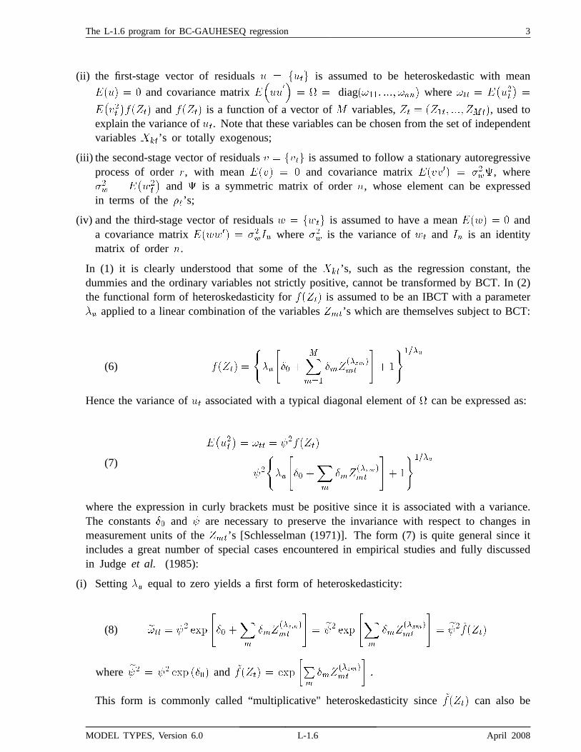
(ii) the first-stage vector of residuals � � ���� is assumed to be heteroskedastic with mean
���� � � and covariance matrix ����
�
�� � � diag����� ���� ���� where ��� � �
������
����������� and ����� is a function of a vector of � variables, �� � ����� ���� ����, used to
explain the variance of ��. Note that these variables can be chosen from the set of independentvariables ��’s or totally exogenous;
(iii) the second-stage vector of residuals � � ���� is assumed to follow a stationary autoregressiveprocess of order , with mean ���� � � and covariance matrix ������ � ����, where��� � �
����
�and � is a symmetric matrix of order , whose element can be expressed
in terms of the ��’s;
(iv) and the third-stage vector of residuals � � ���� is assumed to have a mean ���� � � anda covariance matrix ������ � ����� where ��� is the variance of �� and �� is an identitymatrix of order .
In (1) it is clearly understood that some of the ��’s, such as the regression constant, thedummies and the ordinary variables not strictly positive, cannot be transformed by BCT. In (2)the functional form of heteroskedasticity for ����� is assumed to be an IBCT with a parameter�� applied to a linear combination of the variables ���’s which are themselves subject to BCT:
(6) ����� �
���
��� �
�����
����������
�� �
����
Hence the variance of �� associated with a typical diagonal element of � can be expressed as:
(7)
������� ��� � �������
� ��
���
��� �
��
����������
�� �
����
where the expression in curly brackets must be positive since it is associated with a variance.The constants �� and � are necessary to preserve the invariance with respect to changes inmeasurement units of the ���’s [Schlesselman (1971)]. The form (7) is quite general since itincludes a great number of special cases encountered in empirical studies and fully discussedin Judge et al. (1985):
(i) Setting �� equal to zero yields a first form of heteroskedasticity:
(8) ��� � �� �
��� �
��
����������
�� �� �
���
����������
�� �� ������
where �� � �� � ���� and �� ���� � �
�����
�������
��
This form is commonly called “multiplicative" heteroskedasticity since ������ can also be
MODEL TYPES, Version 6.0 L-1.6 April 2008

4 The L-1.6 program for BC-GAUHESEQ regression
expressed as a product of M exponential functions, or equivalently the logarithm of the variance���� is a linear combination of the �
������� ’s:
(9) ���� � �����
�������
�������
�
(10) � �� ���� � �� ��� ���
���������� � ��� ��
�
����������
where ��� � �� ��� � ���� � �� �
Harvey (1976) considered a special case of (9) - (10) where every ��� is set to one:
(11) ���� � �����
��� ������ � �� ������
�
��� ������
(12) � �� ���� � ��� ���
����� � � � ���� ���
�����
where����
� �����
��� ���� and ���� � ��� ���
�� � Another special case of (9) - (10) can
be obtained if every ��� is set equal to zero:
(13) ���� � �����
��� �������� � �����
���
��
(14) � �� ���� � �� ��� ���
�� ����� � ��� ���
�� �����
which was considered by Dagum and Dagum (1974). The univariate case (M=1) has beenoften used in practice, for example in Geary (1966), Park (1966), Kmenta (1971) or Glejser(1969) who has proposed in his test for heteroskedasticity specific values of �� such as 2, 1,1/2, –1/2 and –1 to give what he called “pure” heteroskedasticity.
(ii) A second form of heteroskedasticity corresponds to the case where �� �� . An importantcase found in the literature [Hildreth and Houck (1968), Theil (1971), Goldfeld and Quandt(1972), Froehlich (1973), Harvey (1974), Amemiya (1977)] corresponds to the special casewhere �� and every ��� are set equal to one, i.e. where the variance ��� is assumed to bea linear combination of the ���’s:
(15)
���� � ��
��� �
��
����� � � �
�
� ��
�� �
��
�� �
���
�������
� ��� ���
������
where ��� � ��
��� �
��
�� �
�and ��� � ����.
MODEL TYPES, Version 6.0 L-1.6 April 2008

The L-1.6 program for BC-GAUHESEQ regression 5
For the univariate case (M=1), Glejser (1969) considered the cases where �� � � and 2 with��� � �, and also the subcases which he called “mixed" heteroskedasticity corresponding to�� � � and 1/2 with ��� � �� � �. Due to the positivity constraint on the diagonal elementsof � in the special form (15) as well as in the more general form (7) with �� �� �, it is hard toestimate the �-coefficients and �-parameters without violating the constraint, as experienced inpreliminary tests with an earlier version of our computer program. Therefore, in this programversion, we will only consider the first form of heteroskedasticity (8) with �� � � which stillincludes a great number of interesting cases.
B. Likelihood function
Before considering the likelihood function for the observed ��’s, it is convenient to rewrite themodel (1)-(2)-(3) into a more compact form where various expressions which will be frequentlyused throughout the manual will be defined. The equation (3) for the residuals ��’s can beexpressed as a function of the residuals ��’s given in (2):
(16)��
��������
���
������
����������
� ��
where ����� � ������ � �
������
�������
�following (8). Replacing �� which is derived from
(1) as � ����� �
���
������� and ���� by an analogous expression in � � � yields:
(17)
������
�����������
�
�������
��������
���
���
�������
�������������
���
��
����������
����������
� ��
� �
� ���
��
�� ���
����
��� ���
���
���
����� � ��
where � �
� � ������ �����
��� and �
�� � ������� �����
���. The corresponding expressions for� � � are obtained by replacing � by � � �. The resulting form (17) can be more compactlyrewritten as:
(18)� �
� ���
����
��� ���
�
��
�� ���
���
�����
�� ��
� ��
� ���
���
�� � ��
where � ��
� � � �
� ���
����
��� and ��
�� � �
�� ���
���
�����.
Assuming that the residuals ��’s are independently and normally distributed ���� ��
�and
dropping the first � observations to simplify the procedure for higher order autocorrelation,i.e. assuming that the first observations on �� are given, the likelihood function associated withthe last � � � observations on �� can be written as follows:
MODEL TYPES, Version 6.0 L-1.6 April 2008

6 The L-1.6 program for BC-GAUHESEQ regression
(19) � ���
�����
�������
���
��
�������
��������
���
����where the residual �� is given by (18) as � ��
� ���
�����
�� , and the jacobian of the transformation
from �� to the observed �� is: ��������� � ������ �����
��� . The corresponding log-likelihoodfunction is:
(20) � ��
��������
��
�
����
��
��� ��
�
��
� ���� ��� � ����
���
where � � � � and the index � for the summation runs from � � to . Note that this
function depends on all the parameters of the model: � ��
�
� ���� ��� ��
�� ��
� ��
� ��
�
where ���and �� are scalars, and �� ��� �� � and � are the column vectors associated with the ��’s, ���’s,�’s, �’s and ��’s respectively.
C. Concentrated log-likelihood function
Since the model (18) rewritten in terms of the transformed variables � ��
� and ���
�� ’s is just linearin the �-coefficients, we can concentrate the log-likelihood function on the ��’s and ��� bysetting the first derivatives of the function with respect to these parameters to zero and solvingfor their values which will be replaced in (20). In matrix notation, the compact form (18) canbe expressed as:
(21) � �� � ���� �
where in view of (19) and (20), � �� is a column vector containing the last � observations, ��� isan �� ��� matrix, � is a �� � �� vector of coefficients and � is an �� � �� vector of residuals.
Using (21) to replace����� in the log-likelihood function (20) by ���, the first derivatives of
the function with respect to � and ��� are given by:
(22)
�
��� �
�
����
����
��� �
�
���
��� �� �������
���� �� ������
��
������
�
�� �� ������ ��
���
���
�
� �� �����
����
(23)
�
����� �
�
�
�
���
�
�������
��
����
���
�
������
��
By equating these two derivatives to zero and solving for � and ���, we obtain:
MODEL TYPES, Version 6.0 L-1.6 April 2008

The L-1.6 program for BC-GAUHESEQ regression 7
(24) �� �����
�
���
���
����
� ��
(25) ���� ��
���� �
�
��� ��
��������� ��
������
Replacing � by �� in (25) gives a value of ��� in function of ��:
(26) ���� ��
�
�� ��
���� �����
� ������ ��
��
Substitution of �� and ���� in � yields the concentrated log-likelihood function:
(27) �� � ��
��� � ������
�
� ���� �
�
�
��
��� � ��� � ����
��
which now depends only on �� ����� �
�
�� ��
�� �
� ��
��
�
1.3 Computational aspects
A. Maximization procedure
The Davidon-Fletcher-Powell (DFP) algorithm [Fletcher and Powell (1963)] is used to maximize
the concentrated log-likelihood function �� with respect to �� ����� �
�
�� ��
�� �
� ��
��
. The gradient
of �� which is used in DFP can be written as:
(28)� ��
� ��� �
�
����
��
��
���
� ���
�
�
��
� ���
� ������� � ��
� ��
��
��
where
MODEL TYPES, Version 6.0 L-1.6 April 2008

8 The L-1.6 program for BC-GAUHESEQ regression
(29)���
����
�
� �������
�������
����
��
��
����������
���������
���
(30)���
����� ���
�� �
��������
���������
�����
��
��
����������
������������
����
��
(31)���
���� �
�
�
�� �
��������
��������
����
��
�����
����������
�����������
���
��
(32)���
�� �
�
�
��
��������
������� �
��
�����
����������
����������
�
(33)���
���� �
���
����������
(34)� �� �����
� ���
�����
if �� �� �� and �
��
������
���if �� � ���
������� if �� � �
(35)���� � ��
� ���
� if �� �� ���
� if �� � ���
The derivatives �� ����� ��� in (29), �������
�� ���� in (30) and �������� ��� in (31) and (34)
as well as their lagged expressions are computed by the generic formula:
(36)��
����
���
�
��
�� �� ���� � �
����
if � �� �
�� ��
� �� if � � �
MODEL TYPES, Version 6.0 L-1.6 April 2008

The L-1.6 program for BC-GAUHESEQ regression 9
B. Asymptotic covariance matrix of the parameter estimates
At the maximum point of ��, hence L, the asymptotic covariance matrix of all the parameterestimates �� is evaluated by the method of Berndt et al. (1974). The log-likelihood function� in (20) can be rewritten as a sum of � individual log-likelihood functions associated witheach observation �:
(37) � ��
�
�� ��
�
��
�
���������
��
�
������
� ��
��� ����� ��� � �� ���
�
where �� is the log-likelihood function corresponding to the observation t and is equal to theexpression in square brackets. The asymptotic covariance matrix of �� is given by:
(38) Var���� �
���
��
�
��
��
��
����where the column vector ���� has the following form:
(39)��
�� �
�
����
����
�
�
�
���� ��
��
��
�
�
�
�� �����
���� � ��
����
with
(40)�����
�
�� if �� �� ����
� if �� � ����
(41)���� ��
��
���
�
� ����
���
��
��
if �� �� ����
����
���if �� � ����
(42)��
��
�
� ���
���
if �� � ����
� ��
�� if �� � ���
Note that the derivatives ��� ��� in (42) for the typical elements of �� are already given in(29)-(30)-(31)-(32)-(33). Since ����� is a function of the ���’s and ��’s only, the derivative �� �������� is also given in (34) for �� � ��� � ��� and ��. Finally the derivative��� � ����� is equal to zero if �� �� �� and one if �� � �� as in (35).
MODEL TYPES, Version 6.0 L-1.6 April 2008

10 The L-1.6 program for BC-GAUHESEQ regression
C. Scaling of the variables
Although at the initial and final steps of the maximization of ��, all the outputs are given in termsof the original units of the variables ��, ��� and ���, an automatic scaling of these variablesis performed during the iterations to avoid numerical problems which can slow down or inhibitthe convergence process. Each variable �� is scaled as follows:
(43) ��� � ����
where �� represents ��� ��� or ��� in their original units, and �� is the scaling factor of the
form ���
����
�����
����
��in which the square brackets indicate that the greatest integer is being
taken for the expression inside.
In general, the � and �-coefficients and their unconditional t-values computed from (38) are notinvariant with respect to the scaling of ��, ��� and ���, due to the fact that the �-coefficientsdepend on the measurement units of �� and ���’s, and the �-coefficients depend on those of���’s. In contrast, the �� �� � and -parameters as well as their unconditional t-values remaininvariant, since these parameters are pure numbers, i.e. do not depend on the measurement unitsof the variables. Note that the concentrated log-likelihood function ��, hence �, and the errorvariance ��� are affected by the scaling of �� only. Therefore the concentrated log-likelihoodvalues which are listed in terms of the scaled units of �� during the iterations would not be thesame as if they were in the original units of ��, unless the scaling factor of �� happens to beequal to one for a particular data set. When a test for stability of the �-coefficients over variousdata sets is performed in terms of the log-likelihood values or the error variance estimates, thesequantities must be in the original units of ��, or more generally in a system of units which iscommon to all data sets used.
Table 1 summarizes the relationships between the original � and � and the scaled �� and ��, as wellas the original and scaled log-likelihood functions � and �� due to the scaling of the variables ��,���’s and ���’s, when each variable is transformed by Box-Cox. For the dependent variable,due to the Box-Cox transformation, all the �-coefficients including the regression constant, aswell as the log-likelihood function, will change. For the independent variables, only a strictlypositive variable ��� or a quasi-dummy ��, which is defined as a nonnegative variable inSection 2.6, can be transformed by Box-Cox. An associated real dummy � is always createdfor each quasi-dummy ��, since the null observations of �� cannot be transformed by Box-Cox.The main difference between ��� and ��, when they are scaled, is that due to the Box-Coxtransformation, there will be a shift in the regression constant � for ��� and in the �-coefficientof the associated real dummy, ���
, for ��, in addition to the usual changes in the �-coefficientsof ��� and �� themselves. The log-likelihood function will not be affected by the scaling of��� or ��. For the heteroskedasticity variables, only the �-coefficient associated with each ���will change. There will be no effect on the regression constant and the log-likelihood function.
MODEL TYPES, Version 6.0 L-1.6 April 2008

The L-1.6 program for BC-GAUHESEQ regression 11
TABLE 1 Relationships between the original (�� �� �)and scaled (��� ��� ��) for Box-Cox transformed variables.
Variable Regression constant � or �-coefficient Log-likelihood
Dependent��� � ���� ��� � �
��� �� � �
�����
��� � ���� �� for all k’s �� � � �� �� ��
Independent• Strictly positive���� � ������ ��� � �� � �
�������
���������
��� � ���������
�� � �
(invariant)
• Quasi-dummy��� � ���� ��� � �� (invariant) ��
��� ����
���
����� ���
� ������
�������
�� � �
(invariant)
Heteroskedasticity��� � ����� ��� � �� (invariant) ��� � ����
�����
�� � �
(invariant)
D. Constraints on the -parameters
Strictly speaking, the autocorrelation parameters ’s in (3) must satisfy a very large numberof conditions to ensure stationarity in an autoregressive process of order �. For simplicity,a constraint �� � � � on every is implicitly introduced by using the Fisher’s -transformation:
(44) ��
���
� � ��
��� � ���
with the corresponding inverse transformation � �� . This parameter change from to implies that the maximization of �� is performed with respect to the -parameters. Therefore,during the iterations the -values are listed instead of the -values which are only given atthe convergence of �� when all the estimated parameters of the model �� are printed with theirstandard-errors and t-statistics. The derivative of �� with respect to each z-parameter is computedas follows:
(45)� ��
� �
� ��
�
��
where � ���� is already given in (28) and (33), and ��� � sech� � ����� � ��� .
MODEL TYPES, Version 6.0 L-1.6 April 2008

12 The L-1.6 program for BC-GAUHESEQ regression
1.4 Model types
Four types of Box-Cox regression models can be specified using the different options available:
BC. This model type only includes the Box-Cox (BC) transformation on the dependentand independent variables in the regression equation (1) without considering the problemsof heteroskedasticity and autocorrelation for the residuals ��’s and ��’s respectively. Theparameters involved are �� ��
�� �� and �� where the variances of ��� �� and �� are all identical;BC–HE. This model type extends the previous one to the case where the functional form
of HEteroskedasticity (HE) of the first-stage residuals ��’s, � ���� � ���
���
���������
�,
is specified simultaneously with the BC transformation on the dependent and independentvariables. The additional parameters to be considered are the �� and -vectors which areinvolved in �����. Since the problem of autocorrelation of the residuals ��’s is not considered,the variance of �� remains identical to the variance of ��, but the latter is different from thevariance of ��;BC–GAU. This model type allows for a Generalized AUtoregressive (GAU) structure of thesecond-stage residuals ��’s, to be estimated jointly with the BC transformation on the dependentand independent variables, while the first-stage residuals ��’s are assumed to be homoskedastic.Only the -parameters are added to the set of parameters already included in the BC model.Hence the variance of �� is different from the variance of ��, but the latter is identical tothe variance of ��;BC–GAUHE. This model type corresponds to the general case where the first-stage residuals��’s are assumed to be heteroskedastic with a functional form ����� and the second-stageresiduals ��’s follow a stationary autoregressive process of order �. All the parameters of the
model, � ���
�
� ���� ��� �
�
�� ��
�� �
� �
��
, are simultaneously estimated. Therefore the variancesof ��, �� and �� are all different.
The BC–GAUHE model type includes all the first three as special cases provided that:
(i) The same set of dependent and independent variables, Y and X, is used for the estimation ofthe parameters, with the same set of �� and ��-parameters being estimated or fixed acrossthe four model types. For example, if �� or some of the ��-parameters are fixed at zero,then the same constraints should be retained across all the model types;
(ii) The same set of variables Z is specified in the functional form of heteroskedasticity for bothBC-HE and BC–GAUHE, with the same set of �� and -parameters being estimated or fixedin both model types. For instance, if every ��� is set to one, then the same constraintsmust be used in both;
(iii) The same structure of the autoregressive parameters is estimated for both BC–GAU andBC–GAUHE so that the simpler model type is nested in the general model type. Forexample, if BC–GAU includes three estimated -parameters of orders 1, 4 and 12, then thesame structure should be preserved in BC–GAUHE.
Note that the BC–HE and BC–GAU model types are completely different since they are based ondifferent assumptions on the structure of the residuals, hence they cannot be compared betweeneach other, although the simpler BC model type is nested in both provided that the condition(i) is satisfied.
MODEL TYPES, Version 6.0 L-1.6 April 2008

The L-1.6 program for BC-GAUHESEQ regression 13
1.5 Model estimation
Since the four model types presented above are by increasing degrees of nonlinearity in theparameters as the specification of a model under study is allowed to be more and more generalby relaxing the constraints on the parameters of heteroskedasticity or autocorrelation or bothwith respect to the BC model type, a normal procedure to succeed in estimating all the fourmodel types can be suggested as follows:
Step 1. Start the estimation of the model with the BC type. If the number of independentvariables is too large to allow for a distinct BC transformation on each variable, regrouping allthe variables which can be transformed by Box-Cox into a few main categories and specifying one��-parameter for each category of variables will reduce the number of estimated ��-parameters.The program includes two types of constraints on the �� and ��-parameters:
(i) �� and any ��-parameter can be fixed at a constant value instead of being estimated. Thistype of constraint permits specially the estimation of the classical functional forms such asthe linear, semilog and loglinear forms: for example, setting �� equal to zero and every��-parameter to one yields the semilog form;
(ii) �� can be set equal to one of the estimated ��-parameter. This type of constraint is usefulin particular for the case where the model is specified with only one estimated �-parametercommon to all the dependent and independent variables. This form can then be compared tothe linear and loglinear forms considered above.
To improve the specification of the model, three special options are available:
(iii) Detection of multicollinearity among the independent variables � with the correlation matrixand specially with the regression coefficient variance decomposition proportions based on thespectral decomposition of � �� in terms of the original and Box-Cox transformed variables(Section 3.1);
(iv) Graphical analysis of the estimated residuals �� which are plotted by increasing values against avariable �� that is thought to explain the variance of �� in the case of heteroskedasticity whichcan arise not only with the cross-section data but can also be induced by the BC transformationon the dependent variable even with the time-series data (Section 3.2);
(v) Statistical tests of the estimates of the autocorrelation function and the partial autocorrelationfunction at different lags of the residuals ��’s for large time-series samples in order to detectthe most significant orders of autocorrelation (Section 3.3).
Step 2. Proceed with estimation according to the results of the previous analyses:
(i) If the problem of severe multicollinearity among a group of independent variables exists,then it should be first treated before considering the problems of heteroskedasticity andautocorrelation: some of the variables must be dropped from the regression equation (1)or replaced by their proxies, i.e. the variables which are used to explain essentially the samephenomena as the original variables, but which are less collinear among themselves. Themodel with a new specification of the variables is reestimated following Step 1. The wholeprocess is repeated until a satisfying set of independent variables is obtained.
(ii) If only the problem of heteroskedasticity is the most serious, then different types of the“multiplicative" form of heteroskedasticity in (8) can be tried using the BC–HE model typesince the program allows the ��-parameters and the �-coefficients in ����� to be estimated
MODEL TYPES, Version 6.0 L-1.6 April 2008

14 The L-1.6 program for BC-GAUHESEQ regression
or fixed at a constant value. At the end of each estimation, the first special option can beused again to detect multicollinearity among the Box-Cox transformed independent variablescorrected for heteroskedasticity ��
��, and for time-series data, the third special option can alsobe used to analyze the structure of autocorrelation of the estimated residuals ��’s. This willallow us to proceed further with the estimation of the model using the BC–GAUHE type ifautocorrelation is present.
(iii) If only the problem of autocorrelation is important, then using the BC–GAU model type issufficient to improve the specification of the model.
Note that at the end of each estimation with the BC–GAU or BC–GAUHE model types wherethe correction for autocorrelation has been applied with a chosen set of estimated �-parameters,a further check on the estimates of the autocorrelation and partial autocorrelation functions willindicate whether the estimated residuals �� behave approximately as a white noise or otherautocorrelation orders remain to be corrected for.
2. ESTIMATION RESULTS
2.1 Definitions of moments of the dependent variable
In a standard linear regression model where the dependent variable �� is not subject to a Box-Cox transformation, the calculated value of �� is equal to the expected value of ��. In constrast,in a Box-Cox regression model where �� is transformed by Box-Cox, this property no longerholds. In this case, the expected value of �� is more relevant than the calculated value of ��.Moreover, we know that the use of the Box-Cox transformation on the dependent variable willaffect the standard error and the skewness of the distribution of ��. In this section, we willdefine these four elements, namely the calculated and expected values of ��, the standard errorand the skewness of ��.
A. Calculated value of the dependent variable ��
Using the equation (18), the calculated value of the transformed dependent variable � ��
� isobtained by replacing all the parameters of the model by their maximum likelihood estimates:
(46) �����
���
������
��
where
�����
� ����
�
��
��� ���
���
����
� ��������
� ���������
�� �
��� ����������� � ��������
���
MODEL TYPES, Version 6.0 L-1.6 April 2008

The L-1.6 program for BC-GAUHESEQ regression 15
����
�� � ���
�� �
��
��� ���
�����
(47)
���
�� � ��������� � ������
���
���
����� � ������������ �
�����������
������ � ���
���
������������
�
�������� � ���
���
���������������
��
Replacing �����
in the left-hand side of (46) by its expression given in (47), we solve the resultingequation for the calculated value of the original ��:
(48) ��� �
����������� � ��� ������
���
���� ��
�
��� ��
�� ����
��
�������if ��� ��
���
� ���������
�
����� �����������
��� ��
�� ����
��
��if ��� �
�
B. Expected value of the dependent variable ��
Following our approach in which the dependent variable �� is assumed to be censored bothdownwards and upwards, � �� � �, where and � are respectively the lower and uppercensoring points common to all observations in the sample, the generalization of Tobin’s model(1958) to a doubly censored dependent variable yields the following expression for the expectedvalue of ��:
(49) ����� �
����� ��
����� �
��� � �����
������ ����� � �
� ��� �
�����
where ��� is the normal density function of � with zero mean and variance ���:
(50) ��� ������
�
���
�
��
���
��
����� is a function of w:
(51) ����� �
�����������
�� � �������
���
�
����
��� ��
����
�� � �
������if �� �� �
���
������
���
����
�� ����
����������
����
��
�� � �
��if �� � �
MODEL TYPES, Version 6.0 L-1.6 April 2008

16 The L-1.6 program for BC-GAUHESEQ regression
and the generic formula for ����� and ����� is:
(52) ����� �
���������
��� � �
�����������
��
����
��� ���
���
�� if �� �� � �
�� �
�������������
������
��������������
��
�� if �� � � �
Depending on the sign of the BC parameter �� , distinct cases can be derived for ����:
1. �� � �. If � and � tend towards 0 and � respectively, following (52) the limits of �����and ����� can be obtained as:
(53) ��� � ������
����� � ��
�������������
����
��� ���
���
��
and ������
����� ��. This expression is used in the program to compute ��� automatically and
cannot be changed by the user, in contrast to the upper limit in case 3 below, in order to avoidnegative values for some observations in the square brackets found on the first line of (51).Whence the first and last terms in (49) disappear and the expected value of �� reduces to thesecond term which can be written as:
(54) ���� �
��
��
�
������������
2. �� � �. If � and � tend towards 0 and � respectively, then ������
����� � �� and
������
����� � �. Hence the first and last terms in (49) disappear and the expected value of
�� reduces to the second term which can be written as:
(55) ���� �
��
��
������������
3. �� � �. If � tends towards 0, then ������
����� � ��, and the first term disappears. Before
taking the limit of ����� as � tends towards � in the last two terms of (49), the expected valueof �� can be expressed as:
(56) ���� �
������
��
����������� �
��
�����
�������
MODEL TYPES, Version 6.0 L-1.6 April 2008

The L-1.6 program for BC-GAUHESEQ regression 17
If � tends towards �, the limit of ����� has a finite value:
(57) ������
����� � ��
�������������
����
��� ���
�����
��
Hence ������
���
�����
����� does not exist and ����� does not have a finite value. In this case, it
is still possible to obtain an approximation of ����� for every observation provided that the userselects a large value of �, say ��, such that the probability that �� exceeds this upper limit �� willbe negligible, i.e. given the values of � �� ��
��
�� and �� in ������, the value of ����� will be muchsmaller than ��. The value of � can be chosen very approximately without affecting the numericalprecision of �����. By default, the program will generate a value of � determined as follows:
(58) �� � �������
�� ����� �������������
�
where �� is the sample standard error of �� and �� and �� are evaluated at their estimated values.Note that if �� is fixed at a certain value in an estimation run, then this value will be used.
For the three cases of �� , the integrals corresponding to the second term in the general expressionof ����� are numerically computed using the Gauss-Legendre 32-point quadrature. As a samplemeasure of the degree of numerical approximation of ����� for the two cases �� � � and �� � �,the mean probability of �� in the sample to be at the lower limit � if �� � � or at the upperlimit � if �� � � is also computed:
(59) ����� � �� ��
�
��
��
����
�����
and
(60) ����� � �� ��
�
��
�������
�����
where the integrals involving just the normal density function ��� are computed with theformula 26.2.17 in Abramowitz and Stegun (1965). A value of ���� lower than 1% indicatesthat the sample contains practically no limit observations.
MODEL TYPES, Version 6.0 L-1.6 April 2008

18 The L-1.6 program for BC-GAUHESEQ regression
C. Standard error of the dependent variable ��
The standard error of �� is defined as the square root of the variance of �� which is also knownas the second moment of �� centered about the mean �����:
(61) ����� ��
Var���� �
����� � ������
� �
���� �
�
�� �������
�
where the first and second noncentral moments ��� �� �, � � �� �� are given by:
(62) ��� �� � �
�������������������
����
�
� �� ��������� if �� �
����
� �� ��������� if �� � �
��������
� �� ��������� � �
�������
������ if �� � �
�
D. Skewness of the dependent variable ��
Skewness is a measure of asymmetry of a distribution. It indicates how the data are distributedin a particular distribution relatively to a perfectly symmetric one. Several types of skewnesscan be defined, but the most usual one is the Fisher Skewness defined as:
(63) ���
�����
���
��
where �� and �� are respectively the second and third moments centered about the mean of thedistribution, and �
���� � � is the standard error of the distribution. Note that the third moment
�� is expressed in cubic units. In order to compare the results from one distribution to another,the skewness is expressed in standard units, i.e. as the third moment divided by ��. It does notdepend on the units of measurement of the variable considered in the distribution. For example,the skewness of a normal distribution is zero because it is symmetric about its mean, whereasa lognormal distribution has positive skewness, i.e. the right tail is longer than the left one.Conversely a negative skewness indicates that the left tail is longer than the right one. Usuallya distribution is considered to be:
Slightly asymmetric, if � � � �� �
Moderately asymmetric, if �� � � � � � �
Highly asymmetric, if � � � �
MODEL TYPES, Version 6.0 L-1.6 April 2008
The L-1.6 program for BC-GAUHESEQ regression 19
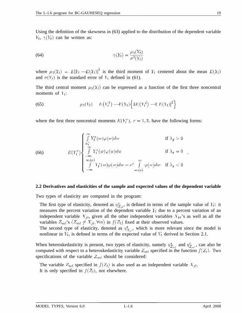
Using the definition of the skewness in (63) applied to the distribution of the dependent variable��, ����� can be written as:
(64) ����� �������
������
where ������ � ���� � ������� is the third moment of �� centered about the mean �����
and ����� is the standard error of �� defined in (61).
The third central moment ������ can be expressed as a function of the first three noncentralmoments of ��:
(65) ������ � ��� �
�
�� �����
����� �
�
�� ��������
��
where the first three noncentral moments ��� �� �� � � �� �� have the following forms:
(66) ��� �� �
�������������������
����
�
� �� �������� if � � �
����
� �� �������� if � � �
��������
� �� �������� ��
�������
����� if � �
�
2.2 Derivatives and elasticities of the sample and expected values of the dependent variable
Two types of elasticity are computed in the program:
The first type of elasticity, denoted as �����, is defined in terms of the sample value of ��: it
measures the percent variation of the dependent variable �� due to a percent variation of anindependent variable ���, given all the other independent variables ���’s as well as all thevariables ��’s ��� �� ������� in ����� fixed at their observed values.The second type of elasticity, denoted as ����
, which is more relevant since the model isnonlinear in ��, is defined in terms of the expected value of �� derived in Section 2.1.
When heteroskedasticity is present, two types of elasticity, namely �����and ����
, can also becomputed with respect to a heteroskedasticity variable �� specified in the function �����. Twospecifications of the variable �� should be considered:
The variable �� specified in ����� is also used as an independent variable ���.It is only specified in �����, not elsewhere.
MODEL TYPES, Version 6.0 L-1.6 April 2008

20 The L-1.6 program for BC-GAUHESEQ regression
A. Derivatives and Elasticities of the Sample Value of ��
The sample value of �� has the same form as ����� in (51), but with � replaced by ��. Thederivative and the elasticity of the sample value of �� with respect to an independent variable��� can be written as:
(67)
�����
����
�����
�
������
����
������� ����
�� ����
�
������
���
����
���
���
�
����
����
����� �����
�
where
(68) �����
���������
� if ���� is not a function of ���
����
�����
�����
����� �
��
����������
�if ���� contains one �� � ���
and �� � ������
��� � �������
�� . Similarly, the derivative and the elasticity of the sample valueof �� with respect to a heteroskedasticity variable �� which appears only in ���� are:
(69)
����
����
�����������
������
�����
���
���
��
������
����
where ���� �
��������
�����
����� �
��
����������
�.
B. Derivatives and Elasticities of the Expected Value of ��
Using ����� in (54)-(55)-(56) depending on the value of � , the derivative and the elasticity ofthe expected value of �� with respect to an independent variable ��� can be written as:
(70)
�����
�������
�����
��
�����������
���
������� ����
�� �������
�������
������������
����
���
������
�
�����
��
�����������
���
����� �����
����������
MODEL TYPES, Version 6.0 L-1.6 April 2008

The L-1.6 program for BC-GAUHESEQ regression 21
where �� is the integration domain of � � ���� ���� ������ and ���� ������ if �� � �� �� � �and �� � � respectively, and
(71) ������� �
������ if ����� is not a function of ����
�����
�����
������
������ � �� ���
����������
�if ����� contains ��� � ���
Likewise, the derivative and the elasticity of the expected value of �� with respect to aheteroskedasticity variable ��� which appears only in ���� are as follows:
(72)
����
�������
����� ���
��
���
���������������
���������
������������
����
���
������
�
�����
���
���������������
���������
where ������� � �
��������
�����
������ � �����
�� �������
�.
C. Derivatives and Elasticities for the Linear and Logarithmic Cases of ��
The most usual forms of the dependent variable �� encountered in pratice are the linear ��� � ��and logarithmic ��� � �� cases:
For these two cases, the explicit forms of the sample value of �� and its derivative andelasticity are given in Table 2, depending on the presence or absence of heteroskedasticity.To be completely general, autocorrelation is considered in these forms which can be furtherreduced in the absence of autocorrelation by setting all the autoregressive coefficients �’sincluded in �� equal to zero.Similarly, for both cases, explicit forms of the expected value of �� and its derivative andelasticity — whenever possible due to the integrals which cannot be reduced to closed forms— are summarized in Table 3.
MODEL TYPES, Version 6.0 L-1.6 April 2008

22 The L-1.6 program for BC-GAUHESEQ regression
TABLE 2 Explicit forms of the sample value of �� and itsderivatives and elasticities for the linear and logarithmic cases of ��.
STATISTIC CASE HOMOSKEDASTICITY HETEROSKEDASTICITY
(No � ���� involved) ��� �� ��� ��� � ���
SAMPLEVALUE
�� � � � � �� � � ��������
��
��
�� � � ��� ���� ���������
�����
�
DERIVATIVE
�� � � ���������� ���
������� � ���
������
�����
�� � � ���������� ��
����
������� � ���
������
���
�� � � Not applicable ���������
Same as above
�����
�� � � Not applicable ���������
�� Same as above
ELASTICITY
�� � � �������� ��
����
����� � ����
���
����
�� � � ����� ���
� �������� ���
����� � ����
�� � � Not applicable ������ Same as above
����
�� � � Not applicable ����Same as above
where �� ��
���
�� ���
�����
�� and ����� �
���������
������
����� �
��
����������
�.
MODEL TYPES, Version 6.0 L-1.6 April 2008

The L-1.6 program for BC-GAUHESEQ regression 23
TABLE 3 Explicit forms of the expected value of �� and itsderivative and elasticity for the linear and logarithmic cases of ��.
STATISTIC CASE HOMOSKEDASTICITY HETEROSKEDASTICITY
(No � ���� involved) ��� �� ��� ��� � ���
EXPECTEDVALUE
�� � � ����� �����
�
�����������
where ����� � � � � �� where ����� � � � ���������� ���
����� LIMIT CASE �����
���
����� � � �� LIMIT CASE �����
��������� � � � �����
����
�� � � ����� �����
�����������
where ����� � � �� � �� where ����� � �������
����� ����
DERIVATIVE
�� � � ����
� ����������
����
�
������Same as left column��
����� � ��
���� LIMIT CASE ���
��
��������
� ����������
LIMIT CASE �����
����
����
�
���������� � ��������
�� � � ����
� ���������� �����
Same as left column��
����� � ��
�� � � Not applicable ���
��� � �� Same as above
���
�� � � Not applicable ���
��� � �� Same as above
ELASTICITY
�� � � �����
�������
�����
����
�
������same as left column� ���
��� � ��
����LIMIT CASE ���
��
���� ����
���
�����
�� �
LIMIT CASE
�����
����
�����
������� �����
��������� �
�� � � ����� ����
� ��������
Same as left column� ���
��� � ��
�� � � Not applicable ������ � �� Same as above
���
�� � � Not applicable ������ � �� Same as above
where � ���
����
��� ���
�����
�� � ��� ������
�����
������
���� �
��
����������
�,
���
��� � �� � �����
����
�
��������������
����� � �� � �����
����
������������������
������ � �� � �
�����
����
�
���������������
����� � �� � �
�����
����
������������������
and ������ � �
����
�����
������
����� ��� ���
����������
�.
MODEL TYPES, Version 6.0 L-1.6 April 2008

24 The L-1.6 program for BC-GAUHESEQ regression
2.3 Derivatives and elasticities of the standard error of the dependent variable
The concept of elasticity can be extended to the standard error of the dependent variable ��,�����, to give a measure of the percent variation of the standard error of �� due to a percentvariation of an independent variable ��� or a heteroskedasticity variable ��� specified in thefunction �����. Like for the derivatives and elasticities of the sample and expected values of ��,two cases of heteroskedasticity can be distinguished for the derivatives and elasticities of �����:
The heteroskedasticity variable ��� is also used as an independent variable ���.It is specified only in the function �����, not elsewhere.
A. Derivative and elasticity of ����� with respect to an independent variable
The derivative and the elasticity of the standard error of �� with respect to an independentvariable ��� are given by:
(73)�����
�������
�����
�
������
���
�� �
�
�����
� ������������
����
�
������������
����
���
�����
where the derivatives of the first and second noncentral moments ��� �� � � � �, with respect
to ��� are:
(74)���� �
� �
����
�
���
�����������
����
�����
�� ������ ������
������� �
Note that ����� �� and ������ are already defined in (51), (70) and (71) respectively,
and that ������ includes the first case of heteroskedasticity where ��� appears also as a
heteroskedasticity variable ��� used in �����. After some algebraic manipulations, the derivativeand the elasticity of the standard error of �� with respect to ��� can be expressed as:
(75)
�����
��
�����
���
����������� ������� ������
����
������� ������ ���
����������
������
�
� �����
���
����������� ������ �������
����
����� � ���
���������� �
B. Derivative and elasticity of ����� with respect to a heteroskedasticity variable
Since the first case of heteroskedasticity has been previously treated, only the second case where��� appears only in ����� is considered here. The formulas for ��
��and ����
are analogous
to �����
and �����without the terms ���
�����
�� and �������� respectively:
MODEL TYPES, Version 6.0 L-1.6 April 2008
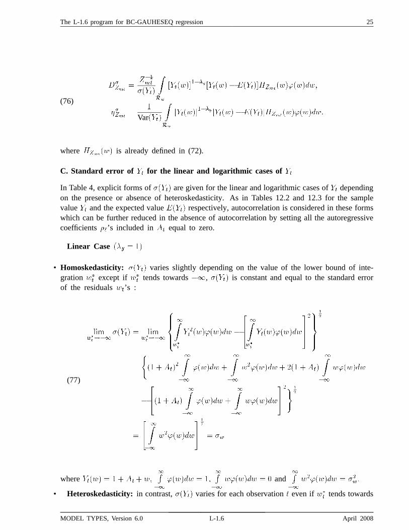
The L-1.6 program for BC-GAUHESEQ regression 25
(76)
�����
������
�����
���
����������� ������� �������������������
���� ��
Var����
���
����������� ������� ��������������������
where ������� is already defined in (72).
C. Standard error of �� for the linear and logarithmic cases of ��
In Table 4, explicit forms of ����� are given for the linear and logarithmic cases of �� dependingon the presence or absence of heteroskedasticity. As in Tables 12.2 and 12.3 for the samplevalue �� and the expected value ����� respectively, autocorrelation is considered in these formswhich can be further reduced in the absence of autocorrelation by setting all the autoregressivecoefficients ��’s included in � equal to zero.
Linear Case ��� � ��
• Homoskedasticity: ����� varies slightly depending on the value of the lower bound of inte-gration ��� except if ��� tends towards ��, ����� is constant and equal to the standard errorof the residuals ��’s :
(77)
�����
����
����� � �����
����
���������
��
�
� �
� ��������� �
�����
��
�
�����������
��������
�
�
�
��� ��
�
����
������
����
�������� �� ��
����
�������
�
���� ��
����
������
����
�������
��� �
�
�
�� ����
��������
�
�
�
� ��
where ����� � � � �����
������ � �����
������� � � and����
�������� � ����
• Heteroskedasticity: in contrast, ����� varies for each observation � even if ��� tends towards
MODEL TYPES, Version 6.0 L-1.6 April 2008

26 The L-1.6 program for BC-GAUHESEQ regression
��. In this case, ����� changes proportionally to ������
� :
(78)
�����
����
����� � �����
����
���������
��
�
� �
� ��������� �
�����
��
�
�����������
��������
�
�
�
��� � �����
�
���
�� ����
������ � �����
����
��������
� ��� � �����
�
���
������
�
�
����
�������
�
���� � �����
�
���
� ����
������ � ������
�
����
�������
��� �
�
�
�������
����
��������
�
�
�
� ������
����
where ����� � � � ������
� ��� � �� �
Logarithmic Case �� � �
• Homoskedasticity: ����� varies proportionally to �� ����:
(79) ����� � �� ����
�����
����
�� ���������� �
�� ����
�� ���������
������
�
�
�
• Heteroskedasticity: ����� is a nonlinear function of �� and ������
� :(80)
����� � ��������
�
���
��������
��
���������
�
��������� �
�� ����
��������
�
���������
������
�
�
�
D. Derivatives and elasticities of ����� for the linear and logarithmic cases of ��
In Table 4, explicit forms of the derivatives and the elasticities of ����� with respect to �� and��� for the linear and logarithmic cases of �� are given in terms of an observation � to showhow both statistics vary with each observation.
a. Derivative and Elasticity with respect to ��
1. Linear Case �� � ��
MODEL TYPES, Version 6.0 L-1.6 April 2008

The L-1.6 program for BC-GAUHESEQ regression 27
• Homoskedasticity: the derivative �����
and the elasticity �����vary slightly depending
on the value of the lower bound of integration ��� , but are both equal to zero as ���
tends towards ��, since �����
����
��
��
�
������� ������������ is equal to zero.
• Heteroskedasticity ���� �� ����: this case is identical to the previous one since theheteroskedasticity function ���� does not include any ��� which is used also as anindependent variable ���.
• Heteroskedasticity ���� � ����: both �����
and �����include two components: one
resulting from the variation of ��� alone and the other from the variation of ���. Inthe limit case where ��� tends towards ��, only the second component remains.
2. Logarithmic Case �� � ��
• Homoskedasticity: the derivative �����
is a function of ��� and �����, but theelasticity �����
is a function of ��� only and it is identical to both elasticities �����
and �����.
• Heteroskedasticity ���� �� ����: this case is identical to the previous one since theheteroskedasticity function ���� does not include any ��� which is used also as anindependent variable ���.
• Heteroskedasticity ���� � ����: the derivative �����
and the elasticity �����depend
on ���� ���� ������ ������ ����� and ��.
b. Derivative and Elasticity with respect to ���
1. Linear Case �� � �
• Homoskedasticity: since ���� is not involved in this case, the derivative ����
andthe elasticity ����
do not apply.• Heteroskedasticity ���� �� ����: the derivative and the elasticity depend on
��� � ���� ������ ������ ����� and ��. If ��� tends towards ��, both statistics
have the same limits as in the case A.1 with heteroskedasticity ���� � ���� sinceonly the heteroskedasticity component remains.
• Heteroskedasticity ���� � ����: this case is identical to the case A.1 with het-eroskedasticity ���� � ����.
2. Logarithmic case �� � ��
• Homoskedasticity: since ���� is not involved in this case, the derivative ����
andthe elasticity ����
do not apply.• Heteroskedasticity ���� �� ����: the derivative and the elasticity depend on
���� ������ ������ ����� and ��.
• Heteroskedasticity ���� � ����: this case is identical to the case a.2 with het-eroskedasticity ���� � ����.
MODEL TYPES, Version 6.0 L-1.6 April 2008

28 The L-1.6 program for BC-GAUHESEQ regression
Table 4 Explicit forms of the standard error of �� and its derivativesand elasticities for the linear and logarithmic cases of ��.
STATISTIC CASE HOMOSKEDASTICITY HETEROSKEDASTICITY
(No ����� involved) ��� �� ��� ��� � ���
STANDARDERROR
�� � ������ �
������
� �
� ����������
������
�����������
������
where ����� � � �� � � where ����� � � � ���������� � ��
����� LIMIT CASE ���������
����� � �� LIMIT CASE ���������
����� � ��������
��
�� � ������ �
�����
� �
� ����������
�����
�����������
������
where ����� � � �� ��� where ����� � �������
����� � ���
DERIVATIVE
�� � �����
����
�����
��
�����
�����
������� ����� ������Same as left column��
����� � ��
����
LIMIT CASE ���������
����
� � LIMIT CASE ���������
����
�
�
� ��
������� �����
�����
�� � � ����
� ��������
�� ����� Same as left column��
����� � ��
�� � � Not applicable ���
��� � �� Same as above
���
�� � � Not applicable ���
��� � �� Same as above
ELASTICITY
�� � ������
����
�����
Var ����
�����
������������ ������same as left column�����
��� � ��
�����LIMIT CASE ���
������
������ � LIMIT CASE
���������
������ �
� ��
�����
�� � � ������ ����
� ������ ���
�����
Same as left column�����
��� � ��
�� � � Not applicable ������� � �� Same as above
����
�� � � Not applicable ������� � �� Same as above
where � ���
����
��� ��
� ���
� �,
���
��� � �� �����
�����
�����
���������������������������
�����
��� � �� ����
��
�����
����
������������ ��������������������
������� � �� � �
Var ����
�����
���������������������������
������� � �� � �
Var ����
����
�������������������������������
and ������� � �
���
�����
������
���� � �����
��������
�.
MODEL TYPES, Version 6.0 L-1.6 April 2008

The L-1.6 program for BC-GAUHESEQ regression 29
2.4 Derivatives and elasticities of the skewness of the dependent variable
A. General caseSince an independent variable ��� can also appear as an heteroskedasticity variable ��� in theheteroskedasticity function �����, two cases for the derivatives and elasticities of ����� can beconsidered:
1. The independent variable ��� also appears in �����. The derivative and the elasticity of����� with respect to an independent variable ��� can be obtained as:
(81)�����
�������
����
��
������
��������
����
� ������������
����
�
����
�������
����
���
�����
Using (65), the derivative of ������ with respect to ��� can be written as:
(82)�������
����
���
�� �
�
�����
�
�������
����
���
�� �
�
�� ��������
�
�� �����
����
�� �
�
�����
� ������������
����
�
The derivative of ������ with respect to ��� is:
(83)�������
����
� �������������
����
where
(84)������
����
��
������
���
�� �
�
�����
� ������������
����
�
In (82) and (84), the derivatives of the first three noncentral moments of �� with respect to��� are given by:
(85)���� �
� �
����
� �
��
���� �����
����
�����
�� ������ ����� �
��� �� � �� � �� ��
where ��� � is defined in (51) and the heteroskedasticity term ����� � in (71). Note that for the
special case where ��� is not specified in �����, then the heteroskedasticity term ����� � is null.
2. The heteroskedasticity variable ��� appears only in �����. The derivative and the elasticityof ����� with respect to ��� are analogous to (81) with ��� replaced by ���:
(86)�����
�������
�����
�
������
��������
����� �����
�������
����
�
����
�������
����
���
�����
MODEL TYPES, Version 6.0 L-1.6 April 2008

30 The L-1.6 program for BC-GAUHESEQ regression
The derivatives of the first three noncentral moments of �� with respect to ��� are given by:
(87)���� �
� �
����� ������
���
���������������
��������� �� � � ��
where ������� is defined in (72).
B. Derivatives and elasticities of ���� for the linear and logarithmic cases of ��For the linear case of the dependent variable, the skewness of �� is zero, since the third centralmoment of �� is equal to zero:
(88) ������ � ���� � ������� � �
��� �
��
�� �������
��� �
����
�� �
where for simplicity, we suppose that �� ���
�� �������
� �� without heteroskedasticity and
autocorrelation. Since the residuals ��’s are normally and independently distributed, all theodd-order moments of �� are zero, in particular the first and third-order moments. Hence thederivative ������� �� as well as the elasticity ��
��are all zero in the linear case of ��. For
the logarithmic case of the dependent variable, there are no closed forms of the skewness ����,the derivatives ��
��and �
����
, and the elasticities ����and �
����
. They should be computednumerically using (64) and (81)-(87).
All these cases are summarized in Table 5.
MODEL TYPES, Version 6.0 L-1.6 April 2008

The L-1.6 program for BC-GAUHESEQ regression 31
TABLE 5 Explicit forms of the skewness of �� and its derivativesand elasticities for the linear and logarithmic cases of ��.
STATISTIC CASE HOMOSKEDASTICITY HETEROSKEDASTICITY
(No � ���� involved) ��� �� ��� ��� � ���
SKEWNESS
�� � � 0
�����
�� � � ����� �������������
���� �
� ������������ �
� ������������
���� �
� �����������
���
where ��� �� �, � � �� �, is given in (66).
DERIVATIVE
�� � � 0 0
��
�� � � ��
��
����
�� � � Not applicable 0 0
���
�� � � Not applicable ���
��
����
ELASTICITY
�� � � 0 0
��
�� � � ��
� ��
��
������
� ���
�� � � Not applicable 0 0
���
�� � � Not applicable
����
���
���
������
� ���
where��
� ��������
� �������
�����������
� ���������������
�as given in (81)
and
���� �����
����� �
������
������������
� ����������������
�as given in (86) .
MODEL TYPES, Version 6.0 L-1.6 April 2008

32 The L-1.6 program for BC-GAUHESEQ regression
2.5 Ratios of derivatives of the moments of the dependent variable
In the three preceding sections, we have considered the derivatives of the three moments of ��
with respect to an independent variable ���, namely ����������� in (70), ����������� in (73)and ����������� in (81). Using these derivatives, three different relations can be obtained forthe ratios of two derivatives of the moments of ��. Consider them in turn:
The ratio of the derivatives of a same moment with respect to two different independentvariables ��� and ��� gives the Marginal Rate of Substitution (MRS) between these twovariables:
(89) ������������
����
������������
�����������
������������
�����������
������������
�����������
This MRS can be shown below to be independent from any moment chosen for the derivatives.
The ratio of the derivatives of two different moments �� and �� with respect to a sameindependent variable ��� gives the Marginal Rate of Substitution (MRS) between those twomoments:
(90) ���� ��� ����
���
���������
��������
� � �� � � �� � and � � ����
where ��, �� and �� represent respectively ������ ����� and �����. It will be shown belowthat this MRS does not depend on any ��� with respect to which the derivatives of themoments are taken.
For two different moments �� and ��, and two different independent variables ��� and ���,we have the following relation for the ratio of derivatives:
(91) ���� ���
��������������
��������
����
���
����
����
���������������
It is a combination of the two preceding cases, i.e. a product of a MRS of moments and aMRS of variables. But the economic interpretation of this case remains to be found.
We therefore focus on the first two ratios and on the elasticity of the second one.
A. Marginal Rate of Substitution between two independent variables
The marginal rate of substitution between two independent variables ��� and ��� can be computedfrom the ratio of the derivatives of the first moment ����� with respect to ��� and ���. It willbe shown below that this MRS does not depend on any moment chosen for the derivatives inthe ratio. Since the independent variables ��� and ��� may also appear in the heteroskedasticityfunction �����, two cases of the MRS between ��� and ��� can be considered:
����� is not a function of ��� and ���. Using (85) for the expressions of the derivatives of����� with respect to ��� and ���, where the heteroskedasticity terms ����
��� and �������
MODEL TYPES, Version 6.0 L-1.6 April 2008

The L-1.6 program for BC-GAUHESEQ regression 33
are null, the MRS can be written as:(92)
�������������
����
������������
�����������
�
�
��
�������������
������� �����
�
��
�������������
������� �����
���
�������
���������
�
For example, in the context of travel demand, the marginal rate of substitution between traveltime (T) and cost (C), also known as the value of time, can be computed as:
(93)� �
������
�����
� �����
�
����� is a function of both ��� and���. Using (85) again for the expressions of the derivativesof ����� with respect to ��� and ���, where the heteroskedasticity terms ����
��� and �������
are nonnull, the MRS cannot be obtained in closed form, but should be computed numerically:(94)
�������������
����
������������
�����������
�
�
��
�����������
���
������� ������ ����
���������
���
�����������
���
������� ������ ����
���������
�
Two special subcases of (94) can be noted:
a. If only ��� appears in �����, then ������� is null.
b. If only ��� appears in �����, then ������� is null.
Now we turn to the proof for the double equality of the ratios of the derivatives of the momentsof ��:
(95)�����������
�����������
������������
�����������
and
(96)�����������
�����������������������
������������
Using (73) for the expressions of the derivatives of ����� with respect to ��� and ���, the ratioof these derivatives can be written as:
(97)
�����������
�����������
�
�
����
���� �
� �����
� ���������������
�
�����
���� �
� �����
� ���������������
� �
���������
���� �
� �����
����
������ ������
�
���������
���� �
� �����
����
������ ������
�
������������
�����������
since��
�� ��
�����
����
���������
�� ��
�����
����
���������
�� ��
�������
�
MODEL TYPES, Version 6.0 L-1.6 April 2008

34 The L-1.6 program for BC-GAUHESEQ regression
Using (81) for the expressions of the derivatives of ����� with respect to ��� and ���, the ratioof these derivatives can be expressed as:
(98)�����������
�����������
�
�
������
������������
� ����������������
�
�������
������������
� ����������������
� �
�����������
������������
����
�������� �����
�
�����������
������������
����
�������� �����
� �
By noting that
(99)������������
�������������
������������������
�������������������
�����������
�����������
and
(100)�������
����
����
���������������
����
����
���������������
��������
we obtain the equality of the ratios of the derivatives:
(101)�����������
������������
�����������
������������
B. Marginal Rate of Substitution between two momentsSince there are three moments of ��, we have six possible combinations of two different momentsfor the ratio of the derivatives of two moments of �� with respect to a same independent variable���. For each combination, we will show that this ratio is independent from any ��� withrespect to which the derivatives of the moments are taken:
1. MRS between ���� and �����. Using (73) for the expression of the derivative�����������, we can write:
(102)�����
�����������������
�����������
������������
��� ��
������ � ���������������
����������
�
Dividing both the numerator and the denominator by ����������, we obtain:
(103) ���� ������
�������
������
��� ��
�������� �����
�
Clearly, this expression does not depend on any ��� with respect to which the derivativesof the two moments are taken initially.
2. MRS between ���� and �����. Using (81) for the expression of the derivative�����������, we can write:
(104)�����
�����������������
������������
����������
������������� � ��������������������������
MODEL TYPES, Version 6.0 L-1.6 April 2008

The L-1.6 program for BC-GAUHESEQ regression 35
Dividing both the numerator and the denominator by �����������, we obtain:
(105) ������ �������
�������
�����
�������������� �������������������
Clearly, this expression does nor depend on any ��� with respect to which the derivativesof the two moments are taken initially.
3. MRS between ���� and �����. Using (73) and (81) for the expressions of ����������
and ����������� respectively, we can write:
(106)�����
�����������������
�����������
�
���
�� �
�
������ � �����������������
���������
������������ � ������������������������
Dividing both the numerator and the denominator by �����������, we obtain:
(107) ������ ������
�������
��������
�� �
�
��������� ������
�
���������������� ��������������������
Clearly, this expression does not depend on any ��� with respect to which the derivativesof the two moments are taken initially.
We have shown that the ratio is independent from any ��� with respect to which the derivatives oftwo moments are taken for the three cases ������������, ������������� and ������������.The three remaining cases ������������, ������������� and ������������ are just theinverse ratios of the three preceding cases. Furthermore it is interesting to note that the sixMRS’s are interrelated. Using the chain rule, the product of (103) and (107) gives (105):
(108)������
�����
�����
�������
������
�������
Each MRS on the left hand side can then be deduced:
(109)������
������������
������������
������
and
(110)�����
�������������
�������������
������
The inverse cases �������������, ������������ and ������������ can be obtained by takingthe inverse of every component in (108), (109) and (110) respectively. Although the sign ofeach MRS taken separately can be:
Positive, if the derivatives of the two moments with respect to a same independent variable��� have the same sign,Negative, if they have opposite signs,
MODEL TYPES, Version 6.0 L-1.6 April 2008
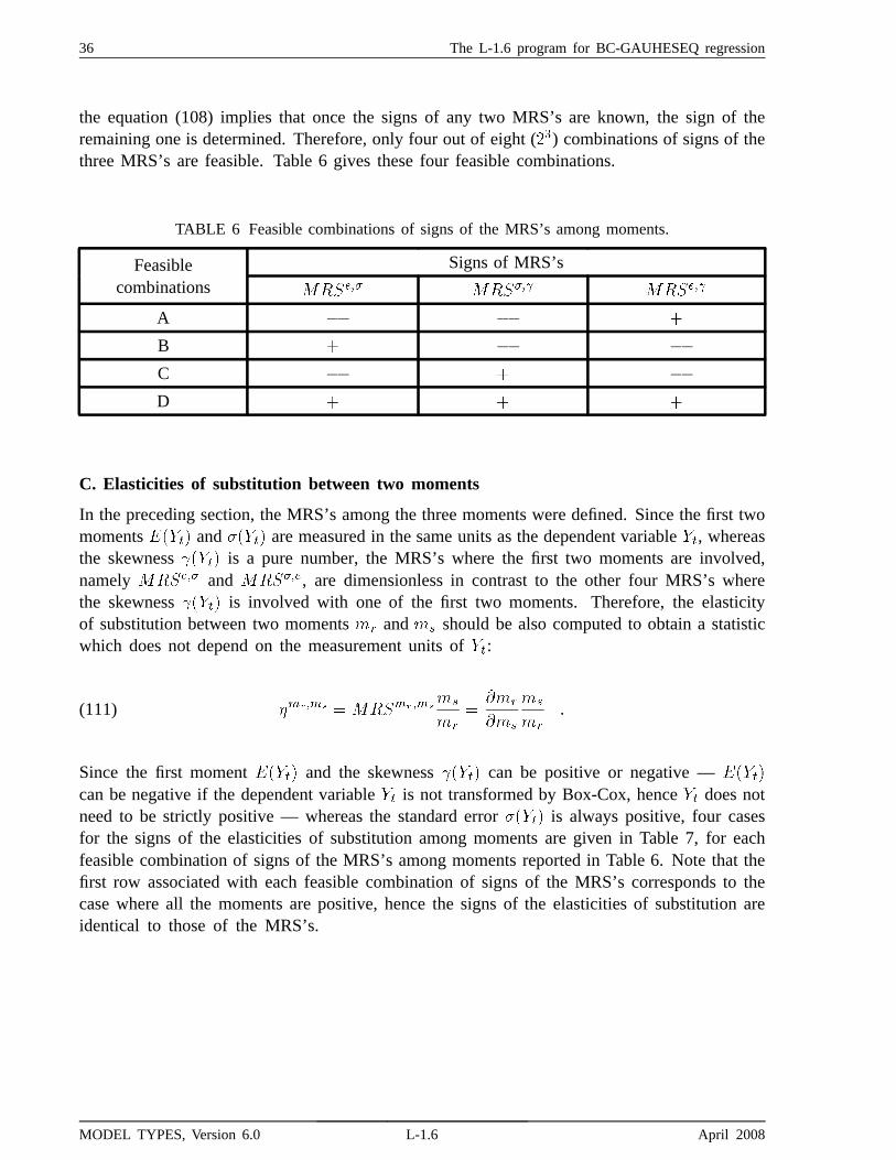
36 The L-1.6 program for BC-GAUHESEQ regression
the equation (108) implies that once the signs of any two MRS’s are known, the sign of theremaining one is determined. Therefore, only four out of eight (��) combinations of signs of thethree MRS’s are feasible. Table 6 gives these four feasible combinations.
TABLE 6 Feasible combinations of signs of the MRS’s among moments.
Signs of MRS’sFeasiblecombinations ������ ������ ������
A � � �
B � � �
C � � �
D � � �
C. Elasticities of substitution between two moments
In the preceding section, the MRS’s among the three moments were defined. Since the first twomoments ����� and ����� are measured in the same units as the dependent variable ��, whereasthe skewness ����� is a pure number, the MRS’s where the first two moments are involved,namely ������ and ������, are dimensionless in contrast to the other four MRS’s wherethe skewness ����� is involved with one of the first two moments. Therefore, the elasticityof substitution between two moments �� and �� should be also computed to obtain a statisticwhich does not depend on the measurement units of ��:
(111) ������ ������ ���
��
��
���
��
��
��
Since the first moment ����� and the skewness ����� can be positive or negative — �����
can be negative if the dependent variable �� is not transformed by Box-Cox, hence �� does notneed to be strictly positive — whereas the standard error ����� is always positive, four casesfor the signs of the elasticities of substitution among moments are given in Table 7, for eachfeasible combination of signs of the MRS’s among moments reported in Table 6. Note that thefirst row associated with each feasible combination of signs of the MRS’s corresponds to thecase where all the moments are positive, hence the signs of the elasticities of substitution areidentical to those of the MRS’s.
MODEL TYPES, Version 6.0 L-1.6 April 2008

The L-1.6 program for BC-GAUHESEQ regression 37
TABLE 7 Feasible combinations of signs of the elasticities of substitution among moments.
Cases Signs of moments Signs of the elasticities of substitutionFeasiblecombinationsof signs of
MRS’se � � ���� ���� ����
A.1 � � � � � �
A.2 � � � � � �
A.3 � � � � � �
A
A.4 � � � � � �
B.1 � � � � � �
B.2 � � � � � �
B.3 � � � � � �B
B.4 � � � � � �
C.1 � � � � � �
C.2 � � � � � �
C.3 � � � � � �C
C.4 � � � � � �
D.1 � � � � � �
D.2 � � � � � �
D.3 � � � � � �
D
D.4 � � � � � �
2.6 Evaluation of moments, their derivatives, rates of substitution and elasticities
A. Evaluation of the moments of ��
In Section 2.1, the expected values of the dependent variable ��, as well as its standard errorand skewness are computed:
For each observation � in the estimation period.For a subset of observations included in the estimation period. Note that this option appliesonly to the expected values of ��.
Note that the calculated value of �� given in (48) is not computed due to the fact that theexpression in the square brackets can be negative and hence cannot be raised to the power ����� ,if ��� �� �.
B. Evaluation of the derivatives and elasticities of ��
MODEL TYPES, Version 6.0 L-1.6 April 2008

38 The L-1.6 program for BC-GAUHESEQ regression
In Sections 2.2, 2.3 and 2.4, the derivatives and elasticities of the sample and expected valuesof ��, and those of the standard error and skewness of �� are computed:
At the sample means of the dependent and independent variables, and the heteroskedasticityvariables if any, for the estimation period.At the sample means of these variables, for a subset of observations included in the estimationperiod. Note that this option applies only to the sample and expected values of ��.
C. Corrected elasticities for a quasi-dummy and a real dummy
The concept of a derivative, hence an elasticity, strictly implies that an independent variableis of continuous type. Since all the independent variables specified in a model may not benecessarily continuous, a classification of the variables into four categories is needed to allowfor the correction of the elasticities for the positive observations of two categories of variables,namely the “quasi-dummies” and the real dummies:
Category 0: Continuous variable which is strictly positive, hence can be transformed by Box-Cox.
Category 1: Any continuous variable which is not strictly positive, hence cannot be transformedby Box-Cox.
Category 2: Quasi-dummy, i.e. a continuous variable containing only positive and null values,for example the level of snowfall per month, which is positive in winter, but null in summer.Strictly speaking, this type of variable cannot be transformed by Box-Cox due to the null values,but if a Box-Cox transformation is absolutely necessary, then only the positive observationsof the quasi-dummy are transformed. Since the null observations cannot be transformed, anassociated real dummy, which has a value of 1 for the positive observations of the quasi-dummyand a value of 0 otherwise, must also be created and specified in the regression equation.
Category 3: Real dummy which has only two values: 0 and a positive constant, for example abinary (0 – 1) variable such as sex (0 for male and 1 for female), or a dummy associated witha quasi-dummy defined above. Unlike a quasi-dummy, a real dummy cannot be transformedby Box-Cox since all the values of 1 will be reduced to zero, if they are transformed with anyvalue of the Box-Cox �-parameter, so that the transformed real dummy will contain only nullobservations.
Two cases of the quasi-dummy should be considered:
1. Quasi-dummy not transformed by Box-Cox. The correction of the elasticities for thepositive observations is based on the fact that one is interested in the effect on the dependentvariable only when an activity or a phenomenon represented by the quasi-dummy or thereal dummy really occurs, i.e. when the observations of the dummy are only positive. Thefollowing correction formula considered in Dagenais et al. (1987) is used:
(112) ��� � ��
�������
� ��
�
�
�������
�
�
�
������ ��
�
���
where �� represents �����, �����
, �����or �����
evaluated at the sample means, ��� is the samplemean of a quasi-dummy or real dummy �� computed from the total set of observations used
MODEL TYPES, Version 6.0 L-1.6 April 2008

The L-1.6 program for BC-GAUHESEQ regression 39
in estimation, and ���� is the sample mean computed only from the positive observationsof �� whose number is ��� . Note that for a subset of observations from the total set, thecorrection formula is analogous.
2. Quasi-dummy transformed by Box-Cox. If a quasi-dummy, say ��, is transformed by Box-Cox, the correction will change slightly for ����
since the expected value of �� evaluated atthe sample means of � and � , say ������ ��� �� , should be computed in fact from the samplemean of a strictly positive variable ��
� instead of �� so that the well-known properties,namely ������ ��� �� � �� and ����
� ��� �� � ����
� ��� �� in the standard linear regression case, maybe preserved. Transforming only the positive observations of �� by Box-Cox while leavingthe null observations of the variable untouched is exactly equivalent to applying the Box-Cox transformation on a strictly positive variable ��
� such that ��
� is identical to �� for theportion of positive observations ��
� and ��
� is equal to 1 for the portion of null observations
of ��, since ������� � �, if ��
� � � for any value of ��. Thus, the correction formula inthis case has the following form:
(113) ����� ����
���
���
� ����
����� ��
��
����
���� ����
�
���
����
��
���� ���
��
�
where ���� is evaluated at the sample means of � and � , with the mean of � replacedby the mean of ��, and ��
� and ��� are respectively the numbers of positive and null
observations of ��.
MODEL TYPES, Version 6.0 L-1.6 April 2008

40 The L-1.6 program for BC-GAUHESEQ regression
TABLE 8 Correction of the elasticities �����
, �����, �����
and ��
���at the sample
means, for the positive observations of a quasi-dummy or a real dummy.
CATEGORY ELASTICITY
�����or �����
����������
(2)Quasi-dummy
• No Box-Cox ���
������
������
���
• With Box-Cox���
�
���
��
��
����
��� �
��
��
��
�� ���
�
��
�
��
��
��
��
��� �
��
��
��
�� ���
�
��
�
��
��
��
��
��� �
��
��
��
��
(3) Realdummy
• No Box-Cox ���
��
�
���
��
�
���
��
�
where �� represents �����, �����
, �����or �����
evaluated at the sample means, ��� represents���� , ���� , ���� or ��
��evaluated at the sample means, ��
� is the number of positiveobservations ��
�� ’s, ��� is the number of null observations of ��� and � is the total number
of observations�� � ��
� ���
�
�used for estimation.
D. Evaluation of the ratios of derivatives of the moments of �� and elasticities of substitutionamong moments
In Section 2.5, three different relations were obtained for the ratios of two derivatives ofthe moments of ��. The first relation gives the Marginal Rate of Substitution between twoindependent variables, the second the Marginal Rate of Substitution (and elasticity of substitution)between two moments, and the third the product of a MRS of moments and a MRS ofvariables. Since the third relation cannot be interpreted in economic terms, only the first tworelations are computed at the sample means of the dependent and independent variables, and theheteroskedasticity variables if any, for the estimation period.
Table 9 summarizes the evaluations provided for the derivatives and elasticities of the moments,and for the ratios of the derivatives of the moments and their elasticities.
MODEL TYPES, Version 6.0 L-1.6 April 2008

The L-1.6 program for BC-GAUHESEQ regression 41
TABLE 9 Evaluations provided for the derivatives and elasticities of the moments,and for the ratios of the derivatives of the moments and their elasticities.
Evaluation provided
At the sample meansStatisticsEquation #reference
Full set Subset
Corrections forQuasi-dummies
and Real Dummies
Derivative
�����
(67) � �
�����
(70) � �
�����
(73) �
�����
(81) �
Elasticity
�����(67) � � �
�����(70) � � �
�����(73) � �
�����
(81) � �
MRS between variables
��������(89) �
MRS between moments
�������� (90) �
Elasticity of substitution between moments
������ (111) �
2.7 Student’s t-statistics
The t-statistics for the estimated parameters can be computed as follows:
At the initial step of the maximization procedure, only the t-statistics for the estimated �-coefficients conditional upon the initial or fixed values of ��� ��� �� � and can be givensince they are based on the results of a standard regression of the transformed dependentvariable �� on the transformed independent variables ���. Hence these tests are invariantto changes of measurement units in the original variables �� and � .At the convergence of the log-likelihood function, two types of t-statistics can be obtained:
MODEL TYPES, Version 6.0 L-1.6 April 2008

42 The L-1.6 program for BC-GAUHESEQ regression
a. Unconditional t-tests for the estimates of ����� ��� ��� �� � and ��� using the standard errorsderived from the covariance matrix (38) are computed under the null hypothesis that theparameter is equal to zero. These tests are invariant to changes of measurement units inthe original variables ��� and � , except for � and �-coefficients due to the applicationof the Box-Cox transformations on these variables. For the �-parameters, apart from thevalue 0 which corresponds to the logarithmic form of the variable, another interestingvalue to test against is the value 1 since it corresponds to a linear specification of thevariable, hence unconditional t-tests for the estimates of ��� �� and �� are also computedunder the null hypothesis that the parameter is equal to one.
b. To obtain invariant t-tests for the � and �-estimates, which are more reliable in hypothesistesting than the unconditional ones which are not invariant, hence can be boosted at willby a proper choice of measurement units of the variables, a simple procedure is to computethe t-tests for �, �, � and ��� conditionally upon the estimates of ��� �� and �� by usingthe conditional covariance matrix of �, �, � and ��� which is equal to the inverse of
a submatrix derived from the matrix
���
���
�����
���
����� in (38) by deleting the rows and
columns associated with ��� �� and �� (Dagenais et al., 1987).
When the program fails to converge to a maximum point, the covariance matrix of the estimatedparameters cannot be obtained. In this case, the standard errors will be set equal to unity so thatthe final table can be printed to give information about the gradient.
2.8 Goodness-of-fit measures
Two goodness-of-fit measures which indicate the accuracy with which a specified model adjuststo the observed data are given in the program: the �� measure is computed with the expectedvalue of ��, ����, defined in section 2.1 and the �� measure is based on the likelihood ratio teststatistic �. Since both measures are just nonlinear extensions of the standard linear regressioncase, they are called pseudo�� measures.
A. Pseudo-(E)-�
Instead of computing the usual � measure defined for a standard linear regression model:
(114) � � � �
��
��� � ������
�
��� � �
��which can give a negative value in the nonlinear case where the dependent variable �� istransformed by a Box-Cox, since the sum of squares of residuals can be greater than the total sumof squares of �� in deviation around its sample mean �� , we compute the square of the simplecorrelation coefficient between �� and ���� called the Pearson �� like Laferriere (1999):
— unadjusted:
�� �
���
��� � �
������� �� �
����
��� � �
����
������ �� �
�
MODEL TYPES, Version 6.0 L-1.6 April 2008

The L-1.6 program for BC-GAUHESEQ regression 43
(115)
— adjusted:
��
� � ��� � �
� ���
�� ���
�
�where �� is the total number of estimated parameters in �� which includes all the �–coefficientsand a set of estimated parameters in ���� ��� ��� �� ���; and � and �� � are respectively themeans of �� and ����: � �
����� and �� � �
������� . This ��
� measure will
always give values within the range 0 – 1, and will be identical to the usual �� measure if thedependent variable �� is linear (Johnston, 1984).
B. Pseudo-(L)-��
— unadjusted:
(116) ��
� � � � ����
— adjusted:
(117) ���
� � ��� � �
� ���
�����
�
�where � is the ratio of the likelihood function � when maximized with respect to the regressionconstant �� only, to the one with respect to �� as defined above:
(118) � � ����
�����
� �
The ��
� measure always remains inside the interval 0 – 1 since the maximum of � associatedwith �� — which corresponds to the most restrictive model where no independent variablesexcept for the constant term are specified — is necessarily smaller than the maximum associatedwith �� which includes less restricted parameters.
Note that for the standard linear regression case ��� � �� � ����� without heteroskedasticity�� � ����� and autocorrelation �� � �, the two measures, ��
� and ��
� coincide since ����
reduces to the ratio of the unexplained sum of squares to the total sum of squares of �� indeviation form:
(119) ���� �
��
�� ��
� � ���������
��� � �
����
�
�����
�������
�����
�
��
��� � ������
�
��� � �
��where ����� is the calculated value of � ��
� given in (46).
MODEL TYPES, Version 6.0 L-1.6 April 2008

44 The L-1.6 program for BC-GAUHESEQ regression
C. Moments of �� observed and estimated, and of ����� estimatedIn a regression model where a Box-Cox transformation is used on the dependent variable ��,one is interested to see how much the transformation will make the distribution of the expectedvalues of �� close to the distribution of the observed values of ��. The first three moments(mean, standard error and skewness) computed for the observed and estimated ��’s and also forthe expected values of �� given by ����� constitute a set of goodness-of-fit measures. Note thatin column B of Table 10, the three moments of the estimated ��’s are evaluated at the samplemeans of the variables.
TABLE 10 Moments of �� observed and estimated, and of ����� estimated.
(A) (B) (C)
MOMENT MOMENT OF ��
OBSERVEDMOMENT OF ��
ESTIMATED ATTHE SAMPLE
MEANS
MOMENT OF �����ESTIMATED
Mean � � �
�
�
�
�� ����� ��� � � �
�
�
�
�����
Standard error�� �
���
����� ��
���
�����
���� � ����
���������� �
��
���
Skewness
�� � ������
where
�� �
��
����� ��
���
����� ���� � � �����
���� �
where
��
� �
��
���������� �
��
���
3. SPECIAL OPTIONS
3.1 Correlation matrix and table of variance-decomposition proportions
A correlation matrix for the independent variables (excluding the constant) and the depen-dent variable in terms of the original variables �� and � � is always given before the maxi-mization procedure begins. Another correlation matrix in terms of the transformed variables(��� and � ��) is also computed at the maximum of the log-likelihood function. The matricesare stored and output in a lower triangular form where the last row represents the pairwisecorrelations between the dependent variable and each of the independent variables.
To detect the presence of multiple linear dependencies among the original independent variables� , the spectral decomposition of �
�
� is used (Judge et al., 1985). This method is similar to
MODEL TYPES, Version 6.0 L-1.6 April 2008

The L-1.6 program for BC-GAUHESEQ regression 45
the singular value decomposition of the matrix � given in Belsley et al. (1980). The analysis isalso performed for the transformed variables ��� at the maximum of the log-likelihood function.The spectral decomposition of �
�
� is defined as:
(120) ��
� ���
���
������
��
where �� is the �� � �� eigenvector associated with the i-th eigenvalue �� of ��
� and thecolumns of � are scaled to unit length but not centered around their sample means, becausecentering obscures any linear dependency that involves the constant term.
Belsley et al. use a set of condition indexes which is a generalization of the concept of thecondition number of a matrix to detect the presence of near dependencies among the columnsof �:
— Condition number of �: ���� � ��������������, where ���� and ���� are respectively
the greatest and smallest eigenvalues of the ��’s. This number measures the sensitivity of � tochanges in �
�
� or ��
� in linear systems represented by the normal equations ��
�� � ��
� ;— Condition indexes: �� � ���������
��� � � ���� . Note that if �� is equal to ����, then�� has a maximum value which corresponds to the condition number of �: ���� � ����.
To determine which variables are involved in each near dependency, a decomposition of thevariance of ���� � � ����� is performed:
(121) Var���� � ���
��
������
�
The proportion of � ������ associated with any �� is then computed:
(122) ��� ���������
��
��
��
������
�
These results can be summarized in a table of variance-decomposition proportions where theelements in each column are reordered according to the increasing values of the ��’s.
TABLE 11 Eigenvalues of ��� , Condition Indexes of � and Proportions of Var(��).
EIGENVALUE CONDITION VARIANCE-DECOMPOSITION PROPORTIONS
INDEX Var(b1) Var(b2) . . . Var(bK)
�1 (�min)�2
.
.�K (�max)
�1 = �(X)�2
.
.�K = 1
�11
�21
.
.�K1
�12
�22
.
.�K2
. . .
. . .
. . .
. . .
. . .
�1K
�2K
.
.�KK
MODEL TYPES, Version 6.0 L-1.6 April 2008

46 The L-1.6 program for BC-GAUHESEQ regression
The sum of the proportions ���’s in each column associated with Var���� is equal to one. Thefollowing rules of thumb can be used to detect the presence of near dependencies:
1. High values of the condition indexes ��� � ��� signal the existence of near dependencies,while high associated ���’s in excess of 0.5 indicate which variable �� is involved in thecollinear relations.
2. When a given variable �� is involved in several collinear relations, its proportions ���’scan be individually small across the high ��’s. In this case, the sum of these proportionswhich is in excess of 0.5 also diagnose variable involvement.
3.2 Analysis of heteroskedasticity of the residuals
At the initial and final steps of the maximization of the log-likelihood function, the estimatedresiduals of ��� �� and �� are plotted around their means, against the observations ordered byincreasing values of one selected independent variable to provide a graphical analysis of thefunctional form of heteroskedasticity related to this variable.
The residuals in standard units are plotted to scale on the horizontal axis, whereas on the verticalaxis, the independent variable is not, due to the large number of observations: one line representsan observation, irrespective of the real distance between two consecutive observations.
3.3 Analysis of autocorrelation of the residuals
At the initial and final steps of the maximization of ��, autocorrelation and partial autocorrelationfunctions are estimated for a time-series ��� that is produced by a differencing operation appliedto the estimated residuals ��’s which can be the ���’s, ���’s or ���’s depending on which modeltype is specified:
(123) ��� � ������� ������ � �� � � � �� � �
where is the backward shift operator defined as �� � ����, hence ��� � ����, �
is the degree of consecutive differencing �� � � � ��, � is the degree of seasonal differencing�� � � � �� and � is the period of seasonal differencing �� � � � ���. An additional constraintfor ��� and � is � � �� � � �. For example, if only the residuals ��’s are to be analyzed,but not the higher order differences produced by consecutive and/or seasonal differencing, then� and � should be set at 0 and � which is not relevant in this case can be set at any positiveinteger value.
The following estimates are computed for the autocorrelation and partial autocorrelation functionsof ���. (For a complete description and use, see Box and Jenkins (1976)).
A. Estimate of the autocorrelation function
The autocorrelation function is extremely useful in providing a partial description of a stochasticprocess, i.e. a measure of how much correlation, hence interdependency, exists betweenneighboring data points in a time-series. For a normal stationary process ���, the autocorrelationfunction with lag � is defined as:
MODEL TYPES, Version 6.0 L-1.6 April 2008

The L-1.6 program for BC-GAUHESEQ regression 47
(124)
��� ���� ��� � ����� ����� � ������
��� ��� � ��������� ����� � ������
����� ���� ������
���� ����� �
� � �� �� ���� ��
where the mean and variance of ��� are respectively ��� � ������ � �������� and
���� � ��� ��� � ������ � �
�� ����� � ������, and the autocovariance at lag is �� �
�������� ������ � ���������� �������� for any � and �. Note that ��� � � and �� � ����.
The autocorrelation function ����� is dimensionless, i.e. independent of the scale of measurementof the time-series. Since � � ���� � � �� �� ����, all the ���’s lie between �� and 1. It issymmetric about zero, that is ��� � ��
��, hence considering the positive half of the function� � �� is sufficient to analyze the time-series. Since �� � ����� � �������, a normal stationaryprocess ��� is completely characterized by its mean ��� and autocovariance function ����, orequivalently by its mean ���, variance ���� and autocorrelation function �����.
An estimate of the autocorrelation function, called the sample autocorrelation function, canbe computed as:
(125) ��� � ����
�� � �� �� ���� ��
where �� is the estimate of the autocovariance function at lag :
(126) �� ���������
� ��� � ����� ����� � ������� � �� �
��� is the sample mean of ��� computed as��
�����
������� �� and �� is the sample variance of ���
computed as��
�����
� ��� � ��������� ��. Note that for long time-series, the sample autocorrelation
function will closely approximate the true population autocorrelation function, but for smallsamples, e.g. less than 50 observations, it will be biased downward from the latter.
B. Standard error of the autocorrelation estimate
To check whether the theoretical autocorrelation ��� is effectively zero beyond a certain lag �,Bartlett’s (1946) approximation for the variance of the estimated autocorrelation coefficient ofa normal stationary process can be used:
(127) Var����� � �
�
������
����� � ���������� � ������������ � �����������If all the autocorrelations ��� are zero for � � �, all terms except the first between the parenthesesare zero when � �. Thus at lags greater than �, the variance of the sample autocorrelations��� can be expressed as:
MODEL TYPES, Version 6.0 L-1.6 April 2008

48 The L-1.6 program for BC-GAUHESEQ regression
(128) � ������� ��
�
�� � �
�����
�����
� �� � ��
To obtain an estimate of Var(���), say �� �������, the sample autocorrelations ��� � � �� �� � ��are substituted for ���. The square root of this estimate is referred as the large-lag standarderror. For example, if � � �, i.e. the series ��� is assumed to be completely random, then forall lags, the large-lag standard error reduces to:
(129)��� ������� � ��
�
which is printed next to each row of the sample autocorrelations ��� and can be used in a firststep to test the null hypothesis that ��� � �� �� � �� �� �.
A second step would be to select the first lag � at which an autocorrelation coefficient wassignificant and then use (128) to test for significant autocorrelations at lags � longer than�. For example, if ��� were significant, �������� could be tested using the standard error��� � ����
�
������
. For moderate � , the distribution of an estimated autocorrelation coefficient,whose theoretical value is zero, is approximately Normal (Anderson, 1942): on the hypothesisthat ��� is zero, the estimate ��� divided by its standard error will follow approximately a unitNormal distribution.
C. Estimate of the partial autocorrelation function
Whereas the sample autocorrelation function is used as a first guess which is certainly notconclusive for the significance of each autocorrelation coefficient, the partial autocorrelationfunction �� which is based on the fact that for an autoregressive process of order � which hasan autocorrelation function infinite in extent, �� is nonzero for � � � and zero for � � �, i.e.it has a cutoff after lag �, provides a means for choosing which order of autoregressive processhas to be fit to an observed time-series.
Let �� be the �th coefficient in an autoregressive process of order � so that �� is the lastcoefficient. The ��’s can be shown to satisfy the set of equations:
(130) ��� � ������� � ������� � � ������� � �� � �� �� � ��
leading to the Yule-Walker equations:
(131)
���� ��� ��� �������� � ��� �����...
......
...����� ����� ����� �
������ ��
��... ��
��� �
���������...���
���
MODEL TYPES, Version 6.0 L-1.6 April 2008

The L-1.6 program for BC-GAUHESEQ regression 49
The coefficient ���, regarded as a function of the lag �, is called the partial autocorrelationfunction. It measures the correlation between ��� and ����� given ������ � � � � ���������. The esti-
mated partial autocorrelations ����’s can be obtained by substituting the sample autocorrelations���’s for the ���’s in (130) to yield:
(132) ��� � ��������� � ��������� � � � �� ��������� � �� � �� �� � � � � ��
and solving the resulting Yule-Walker equations.
A simple recursive method for estimating the ����’s, due to Durbin (1960), may be used if thevalues of the parameters are not too close to the nonstationary boundaries:
(133) ���� �
�����������������
��� if � � ��
��� � �������
������������
� ��������
����������if � � �� �� � � � � ���
where ���� � ������� � ������������� �� � �� �� � � � � �� �� and �� is the maximum lag of the partial
autocorrelation function. Note that �� should be less than or equal to � which is the maximumlag of the autocorrelation function used in (124).
D. Standard error of the partial autocorrelation estimate
If the process is autoregressive of order , the estimated partial autocorrelations of order � �,and higher, are approximately independently distributed (Quenouille, 1949), and the standarderror for these autocorrelations is:
(134)
��Var����
� ��
�� �� � �
which can be used to check whether the partial autocorrelations are effectively zero after somespecific lag . Note that on the hypothesis that ��� is zero, the estimate ���� divided by itsstandard error is approximately distributed as a unit Normal deviate.
3.4 Forecasting: Maximum likelihood and simulation forecasts
A. Maximum likelihood forecast
To obtain the predicted values of the dependent variable over the periods for � ���� � � � � ���, the following approach is adopted: for the first period of forecast � � �, the maximumlikelihood predicted value of ���� is given by the first order condition ����������� � �, since
maximizing the total log-likelihood function����
�����
�� ���
�����
�� � ���� with respect to ����
MODEL TYPES, Version 6.0 L-1.6 April 2008

50 The L-1.6 program for BC-GAUHESEQ regression
is equivalent to maximizing the log-likelihood function ���� associated with the ��� ��-thperiod only.
The first derivative of the log-likelihood function ���� with respect to ���� can be written as:
(135)
�����
������
�����������
�
����
��� � � �
����
�������������
�����
�����������
��
�������
������������
��if �� �� �
�
����
����
�
�������������
�����
�������������
�������
������������
��if �� � �
where ���� � �������� �
���
�����������
�� �� �. Two subcases must be distinguished:
(i) If �� �� �, setting the derivative equal to zero and solving for � �����, yield an equation of the
second degree in ������:
(136) ������� � �
����� � � � �
where
(137) � �
�� � ��� ���������
����
���
����������
����������
���
��������
������������
����and
(138) � � ������ � ������������
To ensure that the predicted value of ���, say ����, is real and positive, both roots of (136),namely
����� �
�� �
��� � ��
��, must be real, i.e. if �� � �� � �, and the greater
root will be chosen since it will be always positive as shown in the next section. Finally, thechosen root must also satisfy the second order condition ������
���� � �.
(ii) If �� � �, i.e. the dependent variable is specified in a linear form, the first derivative reduces to:
(139) ����
���� � �
�������������
�����
�������������
��������
������������
�which gives a unique maximum likelihood predicted value of ��� by setting the derivativeequal to zero and solving for ���:
(140) ���� � � ���
������������� � �������
�����
��������
������������
MODEL TYPES, Version 6.0 L-1.6 April 2008

The L-1.6 program for BC-GAUHESEQ regression 51
�� � �. Setting the first derivative equal to zero and solving for ���� also give a uniquemaximum likelihood predicted value of ����:
(141) ����� � ���
���
������������� � �������
�����
��������
������������� ����������
��
Note that for all cases, the predicted value �����is computed at � � ��.
Clearly, the approach can be easily extended to the next forecast periods, since in eachsingle period, only the log-likelihood function associated with that period is needed for themaximization, given the sample observed values of the dependent variable in the estimationperiod and its predicted values in the preceding forecast periods. Thus for the -th period offorecast, the predicted value of ���� is also given by the first order condition ��������� � �,subject to the second order condition �������
���� �. The formulas are analogous to (135)
– (141) with � � replaced by � � .
B. Variance of the forecast error
The variance of the forecast error for the first period of forecast, �����, is computed from thecovariance matrix of the parameters � and ����, which is equal to minus the inverse matrix ofthe second derivatives of the total log-likelihood function ���� � ���
������ with respect to �
and ����, evaluated at � � �� and ���� � �����:(142) ������ �
�������� ����
��
��� �����
�� � �
������������
� ��������������
��������������� ���������
����
���
where
������ is the covariance matrix of �� which is already estimated in (38) and is used instead
of �������������
����
which is too complex to be evaluated,
���� is the column vector of covariances between the elements of �� and �����:
(143) ���� � �������
�������
�������
��������
�� ����
���
and ����� is the variance of the forecast error for ����:
(144) ����� � �
�������
�� ����
���
� ��
����������� ���� �
MODEL TYPES, Version 6.0 L-1.6 April 2008

52 The L-1.6 program for BC-GAUHESEQ regression
In general, the variance of the forecast error for the �-th period of forecast, �����
, can berecursively computed from:
(145) ������ �
���������� ����
��
��� �����
�� � �
������������������
�
����� �������������������
���������������
����� �������������
����
where
������ is the covariance matrix of ������� ������ ������ � � � � �������
��
which is already esti-
mated in the preceding period of forecast, and is used instead of ������������������
�
�����
���
which is too complex to be evaluated,���� is the column vector of covariances between the elements of ������� and �����:
(146) ���� � ���������
�������
������������
��������
�� ����
���
and ����� is the variance of the forecast error for ����:
(147) ����� � �
�������
�� ����
���
� ��
�����������������
Note that ������������������� � ������������������ and ������������� � ���������
����,
since ���� appears only in ����. The second derivatives ������������������� and
������������� are in the form � ���
��� �����������
����
times a component which is given
in Table 12 for each element of ���� ���
�
������ ����
��
crossed with ����.
MODEL TYPES, Version 6.0 L-1.6 April 2008

The L-1.6 program for BC-GAUHESEQ regression 53
TABLE 12 Components of the second derivatives of ���� with respect to ���� and ����
���� ����
�� �����������
� ���������
�
��
���
������������
������������
��� ��������
� �������������
������
� ���� ������ �
��
����������
��������
��
��
��
������������
����������
�
�
� ��
��
����������
�����������
��
��
��
������������
�������������
�
�
� ���
�������
����������
�
��
��������
������������
��
����������
��
��
��������
������������
�������������
�
�
�� �
�
�������
����������
�
��
��������
������������
������������ �
��
��������
������������
�������������
�
�� ���������� � �����
������������
������������
��������
������������
������������ � � �� �min�� � �� �� and � � ��
���� �
���
������� �
��������������
����
MODEL TYPES, Version 6.0 L-1.6 April 2008

54 The L-1.6 program for BC-GAUHESEQ regression
In Table 12, the different derivatives ��������� ���� � ��
���������������, and ��
��������������� as well
as their lagged expressions are computed by the generic formula given in (36). In evaluatingthe second derivatives of ���� at the maximum point of the total log-likelihood function���� � ����
����, the predicted values of ������ � � � � ����� obtained by the approach aboveare used just as when the predicted value of ���� is computed, the predicted values of������ � � � � ������� are also used. The error of forecast is computed in percentage whenever theobserved value of the dependent variable is available in the forecast periods � � ��� � � � � �:
(148) �� �
���
��� �
����
where �� and � � are respectively the predicted and observed values of �. The 95% confidence
interval for � is also computed:
(149) �� � ���� � � � �� � ���� where � is estimated from (147).
C. Simulation forecast
In addition to the maximum likelihood predicted value �� �� � � �� � � � � � �, the simulatedvalue of the dependent variable �� is computed at � � as:
(150) �� ���������� � ������
���������
�� � �������
�
�����if �� �� �
�� �����
��������
������������
��� � �������
�
�if �� � �
where ��� is replaced by ���� if ��� is not observed, i.e. if �� � � . Note that for the case�� �� �, if the expression between the squared brackets happens to be negative, then it cannotbe raised to the power ���� and the program will be stopped at that point of the run.
�� �� �. Two subcases should be considered:
Subcase �� �� � : If both ��� and ��� are positive, the bias ��� ����, or equivalently �� ��
� �
�� ��� , can
be shown to be negative if �� � � or �� � � and positive if � � �� � �.
For the first period of forecast � � � � �, if the two roots of (136) are denoted by�� ��� �
��� �
��� � ��
��� and ��� ��
� �
��� �
��� � ��
���, then replacing �� by
its value which is equal to �� ��� in the greater root �� ��
� yields:
(151) �� ��� � �� ��
�
�� �
�� � ����� ���
�
���
MODEL TYPES, Version 6.0 L-1.6 April 2008

The L-1.6 program for BC-GAUHESEQ regression 55
If �� � � or �� � �, then � is negative,�
� � ����� ���� � � and the bias �� ��
� �
�� ��� is
negative. If � � �� � �, then � is positive,�� � ����� ���
� � � and the bias �� ��� �
�� ���
is positive. Furthermore, since �� ��� � �� ��
� ���� ��
� , the bias �� ��� �
�� ��� will be given by the
smaller root ��� ��
� . These results can be illustrated by the following diagrams:
Negative bias : ������ �� ��
� ��� � � or �� � ��
�����
������
�����
| | | | | >
� ��� ��
Positive bias : ������ �� ��
� �� � �� � ��
�����
������
�����
| | | | | >
� ��� ��
Choosing the greater root �� ��� will ensure that the maximum likelihood predicted value of
�� is always positive since the smaller root ��� ��
� can be negative. These results will hold forevery period of forecast � � � � � � � .
Subcase �� � �. : In this case, the bias ������� is null, i.e. the simulated value of the dependentvariable ��� is identical to the maximum likelihood predicted value ��� given in (140):
��� � � � ����������
� ��
�
��� ������
��
��
�
(152) � � � ����������
� �
�� �
��� ������
�
�����
�������
�
��
�
� � ���
���������� � �����
�����
�����
����������
����
MODEL TYPES, Version 6.0 L-1.6 April 2008

56 The L-1.6 program for BC-GAUHESEQ regression
�� � �. In this case, the bias ��� ���� is positive:
(153)
��� � ���
������
���
���
��������
����������
���
�����
��
��
� ���
������
���
���
��
�������
�����������
��
����
�����
����
����
��
��
� ���
���
���������� � �����
�����
������
����������
�� ���
since ��� contains in the argument of the exponential (141) an additional negative term equalto ���
������ .
4. REFERENCES
Abramowitz, M. and I.A. Stegun (1965). Handbook of Mathematical Functions. Dover Pub-lications, New York.
Amemiya, T. (1977). A Note on a Heteroscedastic Model. Journal of Econometrics, 6, 365–370;and “Corrigenda". Journal of Econometrics, 8, 275.
Anderson, R.L. (1942). Distribution of the Serial Correlation Coefficient. Annals of Mathemat-ical Statistics, 13, 1.
Appelbaum, E. (1979). On the Choice of Functional Forms. International Economic Review,20, 449–458.
Bartlett, M.S. (1946). On the Theoretical Specification of Sampling Properties of AutocorrelatedTime Series. Journal of the Royal Statistical Society, Series B, 8, 27.
Belsley, D., E. Kuh and R.E. Welsh (1980). Regression Diagnostics. John Wiley, New York.
Berndt, E.K., B.H. Hall, R.E. Hall and J.A. Hausman (1974). Estimation and Inference inNonlinear Structural Models. Annals of Economic and Social Measurement, 3, 653–665.
Berndt, E.K. and M.S. Khaled (1979). Parametric Productivity Measurement and Choice amongFlexible Functional Form. Journal of Political Economy, 87, 1220–1245.
Blum, U. and M. Gaudry (1999). “SNUS-2.5, a Multimoment Analysis of Road Demand,Accidents and their Severity in Germany, 1968–1989”. Publication CRT-99-07, Centre derecherche sur les transports, Universite de Montreal; Working Paper No. 99-xx, Bureaud’Economie Theorique et Appliquee, Universite Louis Pasteur, Strasbourg; Dresdner Beitragezur Volkswirtschaftlehre Nr. 4/99, Dresden University of Technology, 50 p., May 1999.Gaudry, M. and S. Lassarre, (eds), Structural Road Accident Models: The International DRAGFamily, Elsevier Science, Oxford, Ch.3.
Box, G.P. and D.R. Cox (1964). An Analysis of Transformations. Journal of the Royal StatisticalSociety, Series B, 26, 211–243.
Box, G.P. and G.M. Jenkins (1976). Time Series Analysis: Forecasting and Control, Holden-Day, San Francisco, Revised Edition.
MODEL TYPES, Version 6.0 L-1.6 April 2008

The L-1.6 program for BC-GAUHESEQ regression 57
Dagenais, M.G., M.J.I. Gaudry and T.C. Liem (1980). Multiple Regression Analysis withBox-Cox Transformation and Nonspherical Residual Errors: A Transportation Application.Publication no. 166, Centre de recherche sur les transports, Universite de Montreal.
Dagenais, M.G., M.J.I. Gaudry and T.C. Liem (1987). Urban Travel Demand: The Impact ofBox-Cox Transformations with Nonspherical Residual Errors. Transportation Research, 21B, 6, 443–477.
Dagum, C. and E.B. Dagum (1974). Construction de Modeles et Analyse Econometrique.Cahiers de l’Institut des Sciences Mathematiques et Economiques Appliquees, 8, no. 11–12.
Egy, D. and K. Lahiri (1979). On Maximum Likelihood Estimation of Functional Form andHeteroscedasticity. Economics Letters, 2, 155–159.
Fletcher, R. and M.J.D. Powell (1963). A Rapidly Convergent Descent Method for Minimization.Computer Journal, 6, 163–168.
Froehlich, B.R. (1973). Some Estimators for a Random Coefficient Regression Model. Journalof the American Statistical Association, 68, 329–334.
Gaudry, M. et al. (1993, 1994, 1995, 1996, 1997). Cur cum TRIO? Publication CRT-901.Centre de recherche sur les transports, Universite de Montreal, 20 p.
Gaudry, M.J.I. and M.G. Dagenais (1978). The Use of Box-Cox Transformations in RegressionModels with Heteroskedastic Autoregressive Residual. Cahier no. 7814, Departement desciences economiques, Universite de Montreal.
Gaudry, M.J.I. and M.G. Dagenais (1979). Heteroscedasticity and the Use of Box-Cox Trans-formations. Economic Letters, 2, 225–229.
Gaudry, M.J.I. and J.J. Wills (1978). Estimating the Functional Form of Travel Demand Models.Transportation Research, 12, 253–289.
Geary, R.C. (1966). A Note on Residual Heterovariance and Estimation Efficiency in Regression.American Statistician, 20, (4), 30–31.
Glejser, H. (1969). A New Test for Heteroscedasticity. Journal of the American StatisticalAssociation, 64, 316–323.
Goldfeld, S.M. and R.E. Quandt (1972). Nonlinear Methods in Econometrics, North-Holland,Amsterdam.
Harvey, A.C. (1974). Estimation of Parameters in a Heteroscedastic Regression Model. Euro-pean Meeting of the Econometric Society, Grenoble, France.
Harvey, A.C. (1976). Estimating Regression Models with Multiplicative Heteroscedasticity.Econometrica, 44, 461–465.
Heckman, J. and S. Polachek (1974). Empirical Evidence on the Functional Form of the Earnings-Schooling Relationship. Journal of the American Statistical Association, 69, 350–354.
Hildreth, C. and J.P. Houck (1968). Some Estimators for a Linear Model with RandomCoefficients. Journal of the American Statistical Association, 63, 584–595.
Hollyer, M., W. Maling and G. Wang (1979). Domestic and International Air Cargo Activity.Report no. FAA-AVP-79-10, U.S. Department of Transportation.
Johnston, J. (1984). Econometric Methods, Third Edition, McGraw-Hill, New York.
Judge, G.G., W.E. Griffiths, R.C. Hill, H. Lutkepohl and T.C. Lee (1985). The Theory andPractice of Econometrics, Second Edition, John Wiley, New York.
MODEL TYPES, Version 6.0 L-1.6 April 2008

58 The L-1.6 program for BC-GAUHESEQ regression
Kau, J.B. and C.F. Sirmans (1976). The Functional Form of the Gravity Model: A NewTechnique with Empirical Results. Working paper, Department of Finance, University ofIllinois. Presented at the North American Meeting of the Regional Science Association inToronto.
Kmenta, J. (1971). Elements of Econometrics, Macmillan, New York.
Laferriere, R. (1999). Apply the Pearson Coefficient as a Measure of �� in Nonlinear Models.Publication CRT-99–25, Centre de recherche sur les transports, Universite de Montreal.
Liem, T.C. (1979). A Program for Box-Cox Transformations in Regression Models withHeteroskedastic and Autoregressive Residuals. Publication CRT-134, Centre de recherchesur les transports, and Cahier #7917, Departement de sciences economiques, Universite deMontreal, 60 p.. Refereed in The American Statistician, Vol. 34, no. 2, p. 121, May 1980.
Liem, T.C., Dagenais, M. and M. Gaudry (1983). L-1.1: A Program for Box-Cox Transforma-tions in Regression Models with Heteroskedastic and Autoregressive Residuals. PublicationCRT-301, Centre de recherche sur les transports, and Cahier #8314, Departement de scienceseconomiques, Universite de Montreal, 70 p..
Liem, T.C., Dagenais, M. and M. Gaudry (1987, 1990, 1993). LEVEL: The L-1.4 program forBC-GAUHESEQ regression —Box-Cox Generalized AUtoregressive HEteroskedastic SingleEQuation models. Publication CRT-510, Centre de recherche sur les transports, Universitede Montreal, 41 p.
Liem, T.C., Dagenais, M., Gaudry, M. und R. Koblo (1986). Ein Programm fur Box-Cox Trans-formationen in Regressionsmodellen mit heteroskedastischen und autoregressiven Residuen.Publication CRT-301-D, Centre de recherche sur les transports, Universite de Montreal, andDiscussion paper 4/86, Institut fur Wirtschaftspolitik und Wirtschaftsforschung, UniversitatKarlsruhe, 44 p.
Park, R.E. (1966). Estimation with Heteroskedastic Error Terms. Econometrica, 34, 888.
Quenouille, M.H. (1949). Approximate Tests of Correlation in Time Series. Journal of theRoyal Statistical Society, Series B, 11, 68.
Savin, N.E. and K.J. White (1978). Estimation and Testing for Functional Form and Autocorre-lation: A Simultaneous Approach. Journal of Econometrics, 8, 1–12.
Schlesselman, J. (1971). Power Families: A Note on the Box and Cox Transformation. Journalof the Royal Statistical Society, Series B, 33, 307–311.
Spitzer, J.J. (1976). The Demand for Money, the Liquidity Trap, and Functional Forms.International Economic Review, 17, 220–227.
Spitzer, J.J. (1977). A Simultaneous Equations System of Money Demand and Supply UsingGeneralized Functional Forms. Journal of Econometrics, 5, 117–128.
Theil, H. (1971). Principles of Econometrics, John Wiley, New York.
Tobin, J. (1958). Estimation of Relationships for Limited Dependent Variables. Econometrica,25, 24–36.
Welland, J.D. (1976). Cognitive Abilities, Schooling and Earnings: the Question of FunctionalForm. Working paper 76-14, Department of Economics, McMaster University, Hamilton.
White, K.J. (1972). Estimation of the Liquidity Trap with a Generalized Functional Form.Econometrica, 40, 193–199.
MODEL TYPES, Version 6.0 L-1.6 April 2008

The L-1.6 program for BC-GAUHESEQ regression 59
Zarembka, P. (1968), Functional Form in the Demand for Money. Journal of the AmericanStatistical Association, 63, 502–511.
Zarembka, P. (1974). Transformation of Variables in Econometrics. P. Zarembka (ed.), Frontiersin Econometrics. Academic Press, New York.
MODEL TYPES, Version 6.0 L-1.6 April 2008