less is more: building selective anomaly ensembles · less is more: building selective anomaly...

Less is More: Building Selective Anomaly Ensembleswith Application to Event Detection in Temporal Graphs

Shebuti RayanaStony Brook University

[email protected]

Leman AkogluStony Brook University

[email protected]

AbstractEnsemble techniques for classification and clustering havelong proven effective, yet anomaly ensembles have beenbarely studied. In this work, we tap into this gap and proposea new ensemble approach for anomaly mining, with applica-tion to event detection in temporal graphs. Our method aimsto combine results from heterogeneous detectors with vary-ing outputs, and leverage the evidence from multiple sourcesto yield better performance. However, trusting all the re-sults may deteriorate the overall ensemble accuracy, as somedetectors may fall short and provide inaccurate results de-pending on the nature of the data in hand. This suggests thatbeing selective in which results to combine is vital in build-ing effective ensembles—hence “less is more”.

In this paper we propose SELECT; an ensemble ap-proach for anomaly mining that employs novel techniques toautomatically and systematically select the results to assem-ble in a fully unsupervised fashion. We apply our method toevent detection in temporal graphs, where SELECT success-fully utilizes five base detectors and seven consensus meth-ods under a unified ensemble framework. We provide ex-tensive quantitative evaluation of our approach on five real-world datasets (four with ground truth), including Enronemail communications, New York Times news corpus, andWorld Cup 2014 Twitter news feed. Thanks to its selectionmechanism, SELECT yields superior performance comparedto individual detectors alone, the full ensemble (naively com-bining all results), and an existing diversity-based ensemble.

1 IntroductionEnsemble methods utilize multiple algorithms to obtain bet-ter performance than the constituent algorithms alone andproduce more robust results [5]. Thanks to these advan-tages, a large body of research has been devoted to ensem-ble learning in classification [13, 21, 23, 26] and clustering[8, 11, 12, 25]. On the other hand, building effective ensem-bles for anomaly detection has proven to be a challengingtask [1, 27]. A key challenge is the lack of ground-truth;which makes it hard to measure detector accuracy and toaccordingly select accurate detectors to combine, unlike in

classification. Moreover, there exist no objective or ‘fitness’functions for anomaly mining, unlike in clustering.

Existing attempts for anomaly ensembles either com-bine outcomes from all the constituent detectors [9, 10, 16,19], or induce diversity among their detectors to increase thechance that they make independent errors [24, 28]. How-ever, as our prior work [22] suggests, neither of these strate-gies would work well in the presence of inaccurate detec-tors. In particular, combining all, including inaccurate re-sults would deteriorate the overall ensemble performance.Similarly, diversity-based ensembles would combine inac-curate results for the sake of diversity.

In this work, we tap into the gap between anomaly min-ing and ensemble methods, and propose SELECT, one of thefirst selective ensemble approaches for anomaly detection.As the name implies, the key property of our ensemble is itsselection mechanism which carefully decides which resultsto combine from multiple different methods in the ensemble.We summarize our contributions as follows.• We identify and study the problem of building selective

anomaly ensembles in a fully unsupervised fashion.• We propose SELECT, a new ensemble approach for

anomaly detection, which utilizes not only multipleheterogeneous detectors, but also various consensusmethods under a unified ensemble framework.

• SELECT employs two novel unsupervised selec-tion strategies that we design to choose the detec-tor/consensus results to combine, which render the en-semble not only more robust but improve its perfor-mance further over its non-selective counterpart.

• Our ensemble approach is general and flexible. Itdoes not rely on specific data types, and allows otherdetectors and consensus methods to be incorporated.We apply our ensemble approach to the event detection

problem in temporal graphs, where SELECT utilizes fiveheterogeneous event detection algorithms and seven differentconsensus methods. Extensive evaluation on datasets withground truth shows that SELECT outperforms the averageindividual detector, the full ensemble that naively combinesall results, as well as the diversity-based ensemble in [24].

arX

iv:1

501.

0192

4v1

[cs

.DB

] 8

Jan

201

5

2 Background and Preliminaries2.1 Event Detection Problem Temporal graphs changedynamically over time in which new nodes and edges arriveor existing nodes and edges disappear. Many dynamic sys-tems can be modeled as temporal graphs, such as computer,trading, transaction, and communication networks.

Event detection in temporal graph data is the task offinding the points in time at which the graph structure no-tably differs from its past. These change points may cor-respond to significant events; such as critical state changes,anomalies, faults, intrusion, etc. depending on the applica-tion domain. Formally, the problem can be stated as follows.Given a sequence of graphs {G1, G2, . . . , Gt, . . . , GT };Find time points t′ s.t. Gt′ differs significantly from Gt′−1.

2.2 Motivation for Ensembles Several different methodshave been proposed for the above problem, a survey of whichis given in [3]. To date, however, there exists no singlemethod that has been shown to outperform all the others.The lack of a winner technique is not a freak occurrence.In fact, it is unlikely that a given method could performconsistently well on different data of varying nature. Further,different techniques may identify different classes or typesof anomalies depending on their particular formulation. Thissuggests that effectively combining the results from variousdifferent detection methods (detectors from here onwards)could help improve the detection performance.

2.3 Motivation for Selective Ensembles Ensembles areexpected to perform superior to their average constituentdetector, however a naive ensemble that trusts results fromall detectors may not work well. The reason is, somemethods may not be as effective as desired depending onthe nature of the data in hand, and fail to identify theanomalies of interest. As a result, combining accurateresults with inaccurate ones may deteriorate the overallensemble performance [22]. This suggests that selectingwhich detectors to assemble is a critical aspect of buildingrobust ensembles—which implies that “less is more”.

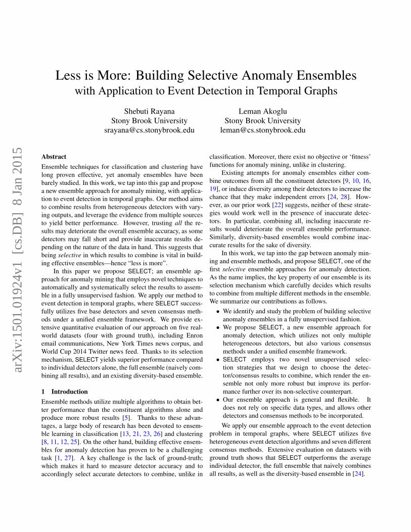
To illustrate the motivation for (selective) ensemblebuilding further, consider the example in Figure 1. Therows show the anomaly scores assigned by five differentdetectors to time points in the Enron Inc.’s time line. Noticethat the scores are of varying nature and scale, due todifferent formulations of the detectors. We realize that thedetectors mostly agree on the events that they detect; e.g., ‘J.Skilling new CEO’. On the other hand, they assign differentmagnitude of anomalousness to the time points; e.g., the topanomaly of methods varies. These suggest that combiningthe outcomes could help build improved ranking of theanomalies. Next notice the result provided by “ProbabilisticApproach” which, while identifying one major event alsodetected by other detectors, fails to provide a reliable rankingfor the rest; e.g., it scores many other time points higher than

Eigen-behaviors

Probabilistic Approach

SPIRIT

Subspace method

Moving Average Z

-sco

re

1 – n

orm

. (s

um

p-v

alu

e)

pro

ject

ion

Time tick

SP

E

Ag

gr.

Dif

f.

Sco

re

J. Skilling

new CEO

Restate 3rd

quarter earning

F. Cooper

new CEO

Figure 1: Anomaly scores from five detectors (rows) for the EnronInc. time line. Red bars depict top 20 anomalous time points.

‘F. Cooper new CEO’. As such, including this detector in theensemble is likely to deteriorate the overall performance.

In summary, inspired by the success of classificationand clustering ensembles and driven by the limited work onanomaly ensembles, we aim to systematically combine thestrengths of accurate detectors while alleviating the weak-nesses of the less accurate ones to build selective detectionensembles for anomaly mining. While we build ensemblesfor the event detection problem in this paper, our approachis general and can directly be employed on a collection ofdetection methods for other anomaly mining problems.

3 SELECT: Selective Ensemble Learning for anomalydetECTion — Application to Event Detection

3.1 Overview Our SELECT approach takes the input data,in this case a sequence of graphs {G1, . . . , Gt, . . . , GT }, andoutputs a rank list R of objects, in this case of time points1 ≤ t ≤ T , ranked from most to least anomalous.

The main steps of SELECT are given in Algorithm 1.Step 1 employs (five) different event detection algorithms asbase detectors of the ensemble. Each detector has a specificand different measure to score the individual time points byanomalousness. As such, the ensemble embodies heteroge-neous detectors. As motivated earlier, Step 2 selects a subsetof the detector results to assemble through a proposed selec-tion strategy. Step 3 then combines the selected results into

a consensus. Besides several different event detection algo-rithms, there also exist various different consensus findingapproaches. In spirit of building ensembles, SELECT alsoleverages (seven) different consensus techniques to create in-termediate aggregate results. Similar to Step 2, Step 4 thenselects a subset of the consensus results to assemble. Finally,Step 5 combines this subset into the final rank list of timepoints using inverse rank aggregation (Section 3.3).

Algorithm 1 SELECT

Input: Data: graph sequence {G1, . . . , Gt, . . . , GT }Output: Rank list of objects (time points) by anomaly

1: Obtain results from (5) base detectors2: Select set E of detectors to assemble3: Combine E by (7) consensus techniques4: Select set C of consensus results to assemble5: Combine C into final rank list

Different from prior works, (i) SELECT is a two-phaseensemble that not only leverages multiple detectors but alsomultiple consensus techniques, and (ii) it employs novelstrategies to carefully select the ensemble components to as-semble without any supervision, which outperform naive (noselection) and diversity-based selection (Section 4). More-over, (iii) SELECT is the first ensemble method for event de-tection in temporal graphs, although the same general frame-work as presented in Algorithm 1 can be deployed for otheranomaly mining tasks, where the base detectors are replacedwith a set of algorithms for the particular task at hand.

Next we fill in the details on the three main componentsof the proposed SELECT ensemble. In particular, we de-scribe the base detectors (Section 3.2), consensus techniques(Section 3.3), and the selection strategies (Section 3.4).

3.2 Base Detectors There exist various methods for theevent detection problem in temporal graphs [3]. In this workSELECT employs five base detectors (Algorithm 1, Line 1),while one can easily expand the ensemble with others: (1)eigen-behavior based event detection (EBED) from our priorwork [2], (2) probabilistic time series anomaly detection (PT-SAD) we developed recently [22], (3) Streaming PatternDIscoveRy in multIple Time-Series (SPIRIT) by Papadim-itriou et al. [20], (4) anomalous subspace based event detec-tion (ASED) by Lakhina et al. [18], and (5) moving-averagebased event detection (MAED). All methods extract graph-centric features (e.g., degree) for all nodes over time and de-tect events in multi-variate time series. We provide brief de-scriptions of the methods in Appendix A due to space limit.

3.3 Consensus Finding Our ensemble consists of hetero-geneous detectors. That is, the detectors employ differentanomaly scoring functions and hence their scores may varyin range and interpretation (see Figure 1). Unifying thesevarious outputs to find a consensus among detectors is anessential step toward building an ensemble.

A number of different consensus finding approacheshave been proposed in the literature, which can be catego-rized into two, as rank based and score based aggregationmethods. Without choosing one over the other, we utilizeseven well-established methods as we describe below.Rank based consensus. Rank based methods use theanomaly scores to order the data points (here, time points)into a rank list. This ranking makes the algorithm outputscomparable and facilitates combining them. Merging multi-ple rank lists into a single ranking is known as rank aggrega-tion, which has a rich history in theory of social choice andinformation retrieval [6]. SELECT employs three rank basedconsensus methods. Kemeny-Young [14] is a voting tech-nique that uses preferential ballot and pair-wise comparisoncounts to combine multiple rank lists, in which the detectorsare treated as voters and the points as the candidates theyvote for. Robust Rank Aggregation (RRA) [15] utilizes or-der statistics to compute the probability that a given orderingof ranks for a point across detectors is generated by the nullmodel where the ranks are sampled from a uniform distri-bution. The final ranking is done based on this probability,where more anomalous points receive a lower probability.The third approach is based on Inverse Rank aggregation, inwhich we score each point by 1

riwhere ri denotes its rank

by detector i and average these scores across detectors basedon which we sort the points into a final rank list.Score based consensus. Rank-based aggregation providesa crude ordering of the data points, as it ignores the actualanomaly scores and their spacing. For instance, quite dif-ferent rankings can yield equal performance in binary de-cision. Score-based aggregation approaches tackle the cal-ibration of different anomaly scores and unify them withina shared range. SELECT employs two score based consen-sus methods. Mixture Modeling [10] converts the anomalyscores into probabilities by modeling them as sampled froma mixture of exponential (for inliers) and Gaussian (for out-liers) distributions. Unification [16] also converts the scoresinto probability estimates through regularization, normaliza-tion, and scaling steps. The probabilities are then compara-ble across detectors, which we aggregate by both max andavg. This yields four score based methods.

3.4 Ensemble Learning Given different base detectorsand various consensus methods, the final task remains toutilize them under a unified ensemble framework. In thissection, we discuss four different approaches for buildinganomaly ensembles. These approaches differ in whether andhow they select their ensemble components.

3.4.1 Full ensemble The full ensemble selects all the de-tector results (Step 2 of Alg.1) and later all the consensusresults (Step 4 of Alg.1) to aggregate at both phases of SE-LECT. As such, it is a naive approach that is prone to obtaininferior results in the presence of inaccurate detectors.

3.4.2 Selective ensembles As motivated earlier in Section2.3, carefully selecting which detectors to assemble in Step 2may help prevent the final ensemble from going astray, pro-vided that some base detectors may fail to reliably identifythe anomalies of interest to a given application. Similarly,pruning away consensus results that may be noisy in Step 4could help reach a stronger final consensus. In anomaly min-ing, however, it is challenging to identify the componentswith inferior results given the lack of ground truth to esti-mate their generalization errors externally. In this section,we present two orthogonal selection strategies that leverageinternal clues across detectors or consensuses and work ina fully unsupervised fashion: (i) a vertical strategy that ex-ploits correlations among the results, and (ii) a horizontalstrategy that uses order statistics to filter out far-off results.Strategy I: Vertical Selection. Our first approach toselecting the ensemble components is through correlationanalysis among the score lists from different methods, basedon which we successively enhance the ensemble one list at atime (hence vertical). The work flow of the vertical selectionstrategy is given in Algorithm 2.

Given a set of anomaly score lists S, we first unifythe scores by converting them to probability estimates usingUnification [16]. Then we average the probability scoresacross lists to construct a target vector, which we treat asthe “pseudo ground-truth” (Lines 1-6).

We initialize the ensemble E with the list l ∈ S thathas the highest weighted Pearson correlation to target. Incomputing the correlation, the weights we use for the listelements are equal to 1

r , where r is the rank of an elementin target when sorted in descending order, i.e., the moreanomalous elements receive higher weight (Lines 7-11).

Next we sort the remaining lists S\l in descendingorder by their correlation to the current “prediction” of theensemble, which is defined as the average probability of listsin the ensemble. We test whether adding the top list to theensemble would increase the correlation of the predictionto target. If the correlation improves by this addition, weupdate the ensemble and reorder the remaining lists by theircorrelation to the updated prediction, otherwise we discardthe list. As such, a list gets either included or discarded ateach iteration until all lists are processed (Lines 12-19).

Strategy II: Horizontal Selection. We are interested infinding time points that are ranked high in a set of accuraterank lists (from either base detectors or consensus methods),ignoring a (small) fraction of inaccurate rank lists. Thus, wealso present an element-based (hence horizontal) approachfor selecting ensemble components.

To identify the accurate lists, this strategy focuses on theanomalous elements. It assumes that the normalized ranksof the anomalies should come from a distribution skewedtoward zero. Based on this, lists in which the anomaliesare not ranked sufficiently high (i.e., have large normalized

Algorithm 2 Vertical SelectionInput: S := set of anomaly score listsOutput: E := ensemble set of selected lists

1: P := ∅2: /* convert scores to probability estimates */3: for each s ∈ S do4: P := P ∪ Unification(s)5: end for6: target := avg(P ) /*target vector*/7: r := ranklist after sorting target in descending order8: E := ∅9: sort P by weighted Pearson (wP ) correlation to target

10: /* in descending order, weights: 1r */

11: l := fetchF irst(P ), E := E ∪ l12: while P 6= ∅ do13: p := avg(E) /*current prediction of E*/14: sort P by wP correlation to p /*descending order*/15: l := fetchF irst(P )16: if wP (avg(E ∪ l), target) > wP (p, target) then17: E := E ∪ l /*select list*/18: end if19: end while20: return E

ranks) are considered to be inaccurate and voted for beingdiscarded. The work flow of the horizontal selection strategyis given in Algorithm 3.

Similar to the vertical strategy we first identify a“pseudo ground truth”, in this case a list of anomalies. In par-ticular, we use Mixture Modeling [10] to convert each scorelist in S into a binary list in which outliers are denoted by 1,and inliers by 0. We then employ majority voting across liststo obtain a final set of target anomalies O (Lines 1-7).

Given that S containsm lists, we construct a normalizedrank vector r = [r(1), . . . , r(m)] for each anomaly o ∈ O,such that r(1) ≤ . . . ≤ r(m), where r(l) denotes therank of o in list l ∈ S normalized by the total numberof elements in l. Following similar ideas to Robust RankAggregation [15], we then compute order statistics based onthese sorted normalized rank lists to identify the lists thatprovide statistically large ranks for each anomaly.

Specifically, for each ordered list l in a given r, wecompute how probable it is to obtain r̂(l) ≤ r(l) when theranks r̂ are generated by a uniform null distribution. Wedenote the probability that r̂(l) ≤ r(l) by pl,m(r). Underthe uniform null model, the probability that r̂(l) is smaller orequal to r(l) can be expressed as a binomial probability

pl,m(r) =

m∑t=l

(m

t

)rt(l)(1− r(l))

m−t,

since at least l normalized rankings drawn uniformlyfrom [0, 1] must be in the range [0, r(l)].

Algorithm 3 Horizontal SelectionInput: S := set of anomaly score listsOutput: E := ensemble set of selected lists

1: M := ∅ , R := ∅ , F := ∅ , E := ∅2: for each l ∈ S do3: /* label score lists with 1 (outliers) & 0 (inliers) */4: class := MixtureModel(l) , M := M ∪ class5: R := R ∪ ranklist(l)6: end for7: O := majorityV oting(M) /*target anomalies*/8: [Ssort, pV als] := RobustRankAggregation(R,O)9: for each o ∈ O do

10: mind := min(pV als(o, :))11: F := F ∪ Ssort(o, (mind + 1) : end)12: end for13: for each l ∈ S do14: count := number of occurrences of l in F15: end for16: Cluster non-zero counts into two clusters, Cl and Ch

17: E := S \ {s ∈ Ch} /* discard high-count lists */18: return E

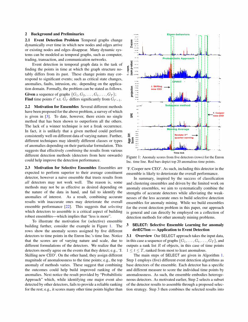
For a sequence of accurate lists that rank the anomaliesat the top, and hence that yield low normalized ranks r(l),this probability is expected to drop with the ordering, i.e., forincreasing l ∈ {1 . . .m}. An example sequence of p proba-bilities (y-axis) are shown in Figure 2 for an anomaly basedon 20 score lists. The lists are sorted by their normalizedranks of the anomaly on the x-axis. The figure suggests thatthe 5 lists at the end of the ordering are likely inaccurate, asthe ranks of the given anomaly in those lists are larger thanwhat is expected based on the ranks in the other lists.

10−3

10−2

10−1

100

10−20

10−15

10−10

10−5

100

r(l)

p l,m(r

)

Figure 2: Normalized rank r(l) vs. probability p that r̂(l) ≤ r(l),where r̂ are drawn uniformly at random from [0, 1].

Based on this intuition, we count the frequency that eachlist l is ordered after the list with minl=1,...,m pl,m(r) amongall the normalized rank lists r of the target anomalies (Lines8-15). We then group these counts into two clusters1 anddiscard the lists in the cluster with the higher average count(Lines 16-17). This way we eliminate the lists with largercounts, but retain the lists that appear inaccurate only a fewtimes which may be a result of the inherent uncertainty ornoise in which we construct the target anomaly set.

1We cluster the counts by k-means clustering with k = 2, where thecentroids are initialized with the smallest and largest counts, respectively.

3.4.3 Diversity-based ensemble In classification, two ba-sic conditions for an ensemble to improve over the con-stituent classifiers are that the base classifiers are (i) accu-rate (better than random), and (ii) diverse (making uncorre-lated errors) [5, 26]. Achieving better-than-random accuracyin supervised learning is not hard, and several studies haveshown that ensembles tend to yield better results when thereis a significant diversity among the models [4, 17].

Following on these insights, Schubert et al. proposed adiversity-based ensemble [24], which is similar to our verti-cal selection in Alg. 2. The main distinction is the ascendingordering in Lines 9 and 14, which yields a diversity-favored,in contrast to a correlation-favored, selection.2

Unlike classification ensembles, however, it is not re-alistic for anomaly ensembles to assume that all the detec-tors will be reasonably accurate (i.e., better than random), assome may fail to spot the (type of) anomalies in the givendata. In the existence of inaccurate detectors, the diversity-based approach would likely yield inferior results as it isprone to selecting inaccurate detectors for the sake of diver-sity. As we show in our experiments, too much diversity is infact bound to limit accuracy for event detection ensembles.

4 EvaluationWe evaluate our selective ensemble approach on the eventdetection problem using five real-world datasets, both previ-ously used as well as newly collected by us, including emailcommunications, news corpora, and social media. For fourof these datasets we compiled ground truths for the temporalanomalies, for which we present quantitative results. We usethe remaining data for illustrating case studies.

We compare the performance of SELECT with verticalselection (SelectV), and horizontal selection (SelectH) to thatof individual detectors, the full ensemble with no selection(Full), and the diversity-based ensemble (DivE) [24]. Thismakes ours one of the few works that quantitatively com-pares and contrasts anomaly ensembles at a scale that in-cludes as many datasets with ground truth.

In a nutshell, our results illustrate that (i) base detec-tors do not always all produce accurate results, (ii) en-semble approach alleviates the shortcomings of the inaccu-rate detectors, (iii) a careful selection of ensemble compo-nents increases the overall performance, and (iv) introducingnoisy results decreases overall ensemble accuracy where thediversity-based ensemble is affected the most.

4.1 Dataset Description In the following we describe thefive real-world temporal graph datasets we used in this work.All datasets with ground truth events are made available athttp://shebuti.com/SelectiveAnomalyEnsemble/.

2There are other differences between our vertical selection (Algorithm2) and the diversity-based ensemble in [24], such as the construction of thepseudo ground truth and the choice of weights in correlation computation.

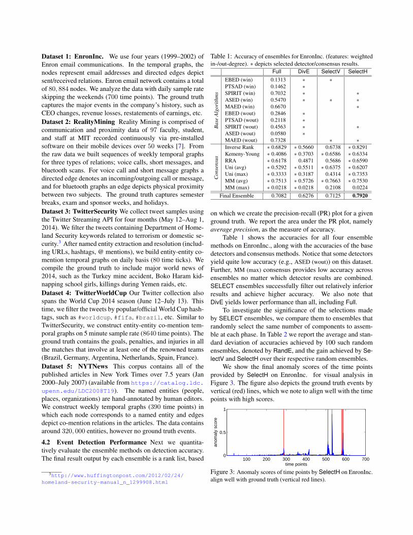
http://shebuti.com/SelectiveAnomalyEnsemble/

Dataset 1: EnronInc. We use four years (1999–2002) ofEnron email communications. In the temporal graphs, thenodes represent email addresses and directed edges depictsent/received relations. Enron email network contains a totalof 80, 884 nodes. We analyze the data with daily sample rateskipping the weekends (700 time points). The ground truthcaptures the major events in the company’s history, such asCEO changes, revenue losses, restatements of earnings, etc.Dataset 2: RealityMining Reality Mining is comprised ofcommunication and proximity data of 97 faculty, student,and staff at MIT recorded continuously via pre-installedsoftware on their mobile devices over 50 weeks [7]. Fromthe raw data we built sequences of weekly temporal graphsfor three types of relations; voice calls, short messages, andbluetooth scans. For voice call and short message graphs adirected edge denotes an incoming/outgoing call or message,and for bluetooth graphs an edge depicts physical proximitybetween two subjects. The ground truth captures semesterbreaks, exam and sponsor weeks, and holidays.Dataset 3: TwitterSecurity We collect tweet samples usingthe Twitter Streaming API for four months (May 12–Aug 1,2014). We filter the tweets containing Department of Home-land Security keywords related to terrorism or domestic se-curity.3 After named entity extraction and resolution (includ-ing URLs, hashtags, @ mentions), we build entity-entity co-mention temporal graphs on daily basis (80 time ticks). Wecompile the ground truth to include major world news of2014, such as the Turkey mine accident, Boko Haram kid-napping school girls, killings during Yemen raids, etc.Dataset 4: TwitterWorldCup Our Twitter collection alsospans the World Cup 2014 season (June 12–July 13). Thistime, we filter the tweets by popular/official World Cup hash-tags, such as #worldcup, #fifa, #brazil, etc. Similar toTwitterSecurity, we construct entity-entity co-mention tem-poral graphs on 5 minute sample rate (8640 time points). Theground truth contains the goals, penalties, and injuries in allthe matches that involve at least one of the renowned teams(Brazil, Germany, Argentina, Netherlands, Spain, France).Dataset 5: NYTNews This corpus contains all of thepublished articles in New York Times over 7.5 years (Jan2000–July 2007) (available from https://catalog.ldc.

upenn.edu/LDC2008T19). The named entities (people,places, organizations) are hand-annotated by human editors.We construct weekly temporal graphs (390 time points) inwhich each node corresponds to a named entity and edgesdepict co-mention relations in the articles. The data containsaround 320, 000 entities, however no ground truth events.

4.2 Event Detection Performance Next we quantita-tively evaluate the ensemble methods on detection accuracy.The final result output by each ensemble is a rank list, based

3http://www.huffingtonpost.com/2012/02/24/homeland-security-manual_n_1299908.html

Table 1: Accuracy of ensembles for EnronInc. (features: weightedin-/out-degree). ∗ depicts selected detector/consensus results.

Full DivE SelectV SelectH

Bas

eA

lgor

ithm

s

EBED (win) 0.1313 ∗ ∗PTSAD (win) 0.1462 ∗SPIRIT (win) 0.7032 ∗ ∗ASED (win) 0.5470 ∗ ∗ ∗MAED (win) 0.6670 ∗EBED (wout) 0.2846 ∗PTSAD (wout) 0.2118 ∗SPIRIT (wout) 0.4563 ∗ ∗ASED (wout) 0.0580 ∗MAED (wout) 0.7328 ∗ ∗

Con

sens

us

Inverse Rank ∗ 0.6829 ∗ 0.5660 0.6738 ∗ 0.8291Kemeny-Young ∗ 0.4086 ∗ 0.3703 ∗ 0.6586 ∗ 0.6334RRA ∗ 0.6178 0.4871 0.5686 ∗ 0.6590Uni (avg) ∗ 0.5292 ∗ 0.5511 ∗ 0.6375 ∗ 0.6207Uni (max) ∗ 0.3333 ∗ 0.3187 0.4314 ∗ 0.7353MM (avg) ∗ 0.7513 ∗ 0.5726 ∗ 0.7663 ∗ 0.7530MM (max) ∗ 0.0218 ∗ 0.0218 0.2108 0.0224

Final Ensemble 0.7082 0.6276 0.7125 0.7920

on which we create the precision-recall (PR) plot for a givenground truth. We report the area under the PR plot, namelyaverage precision, as the measure of accuracy.

Table 1 shows the accuracies for all four ensemblemethods on EnronInc., along with the accuracies of the basedetectors and consensus methods. Notice that some detectorsyield quite low accuracy (e.g., ASED (wout)) on this dataset.Further, MM (max) consensus provides low accuracy acrossensembles no matter which detector results are combined.SELECT ensembles successfully filter out relatively inferiorresults and achieve higher accuracy. We also note thatDivE yields lower performance than all, including Full.

To investigate the significance of the selections madeby SELECT ensembles, we compare them to ensembles thatrandomly select the same number of components to assem-ble at each phase. In Table 2 we report the average and stan-dard deviation of accuracies achieved by 100 such randomensembles, denoted by RandE, and the gain achieved by Se-lectV and SelectH over their respective random ensembles.

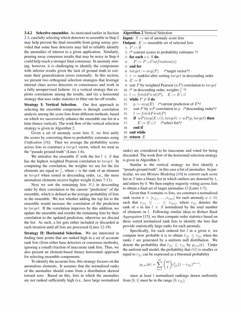
We show the final anomaly scores of the time pointsprovided by SelectH on EnronInc. for visual analysis inFigure 3. The figure also depicts the ground truth events byvertical (red) lines, which we note to align well with the timepoints with high scores.

100 200 300 400 500 600 7000

0.5

1

time points

anom

aly

scor

e

Figure 3: Anomaly scores of time points by SelectH on EnronInc.align well with ground truth (vertical red lines).

https://catalog.ldc.upenn.edu/LDC2008T19

https://catalog.ldc.upenn.edu/LDC2008T19

http://www.huffingtonpost.com/2012/02/24/homeland-security-manual_n_1299908.html

http://www.huffingtonpost.com/2012/02/24/homeland-security-manual_n_1299908.html

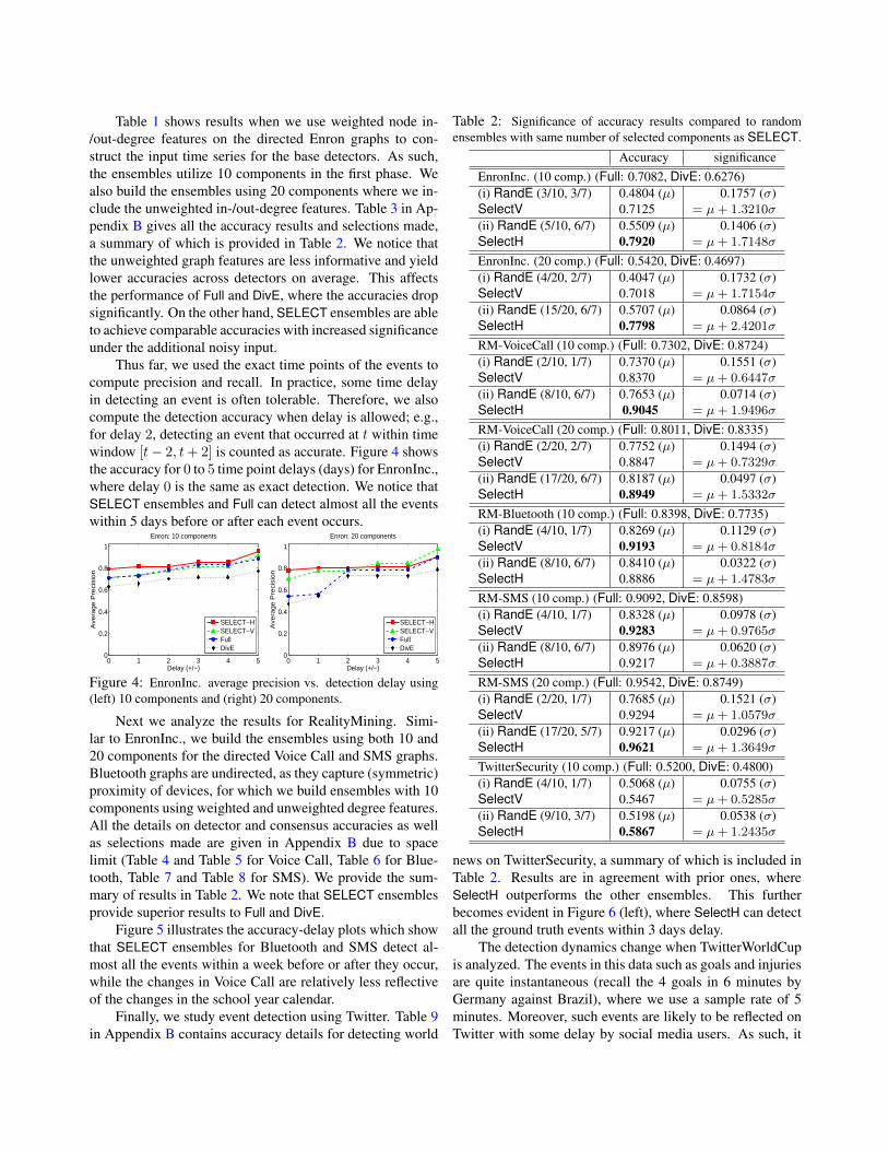
Table 1 shows results when we use weighted node in-/out-degree features on the directed Enron graphs to con-struct the input time series for the base detectors. As such,the ensembles utilize 10 components in the first phase. Wealso build the ensembles using 20 components where we in-clude the unweighted in-/out-degree features. Table 3 in Ap-pendix B gives all the accuracy results and selections made,a summary of which is provided in Table 2. We notice thatthe unweighted graph features are less informative and yieldlower accuracies across detectors on average. This affectsthe performance of Full and DivE, where the accuracies dropsignificantly. On the other hand, SELECT ensembles are ableto achieve comparable accuracies with increased significanceunder the additional noisy input.

Thus far, we used the exact time points of the events tocompute precision and recall. In practice, some time delayin detecting an event is often tolerable. Therefore, we alsocompute the detection accuracy when delay is allowed; e.g.,for delay 2, detecting an event that occurred at t within timewindow [t− 2, t+ 2] is counted as accurate. Figure 4 showsthe accuracy for 0 to 5 time point delays (days) for EnronInc.,where delay 0 is the same as exact detection. We notice thatSELECT ensembles and Full can detect almost all the eventswithin 5 days before or after each event occurs.

0 1 2 3 4 50

0.2

0.4

0.6

0.8

1

Enron: 10 components

Delay (+/−)

Ave

rag

e P

reci

sio

n

SELECT−HSELECT−VFullDivE

0 1 2 3 4 50

0.2

0.4

0.6

0.8

1

Enron: 20 components

Delay (+/−)

Ave

rag

e P

reci

sio

n


Figure 4: EnronInc. average precision vs. detection delay using(left) 10 components and (right) 20 components.

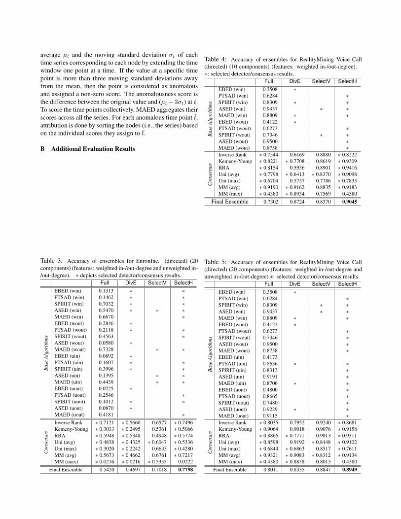
Next we analyze the results for RealityMining. Simi-lar to EnronInc., we build the ensembles using both 10 and20 components for the directed Voice Call and SMS graphs.Bluetooth graphs are undirected, as they capture (symmetric)proximity of devices, for which we build ensembles with 10components using weighted and unweighted degree features.All the details on detector and consensus accuracies as wellas selections made are given in Appendix B due to spacelimit (Table 4 and Table 5 for Voice Call, Table 6 for Blue-tooth, Table 7 and Table 8 for SMS). We provide the sum-mary of results in Table 2. We note that SELECT ensemblesprovide superior results to Full and DivE.

Figure 5 illustrates the accuracy-delay plots which showthat SELECT ensembles for Bluetooth and SMS detect al-most all the events within a week before or after they occur,while the changes in Voice Call are relatively less reflectiveof the changes in the school year calendar.

Finally, we study event detection using Twitter. Table 9in Appendix B contains accuracy details for detecting world

Table 2: Significance of accuracy results compared to randomensembles with same number of selected components as SELECT.

Accuracy significanceEnronInc. (10 comp.) (Full: 0.7082, DivE: 0.6276)(i) RandE (3/10, 3/7) 0.4804 (µ) 0.1757 (σ)SelectV 0.7125 = µ+ 1.3210σ

(ii) RandE (5/10, 6/7) 0.5509 (µ) 0.1406 (σ)SelectH 0.7920 = µ+ 1.7148σ

EnronInc. (20 comp.) (Full: 0.5420, DivE: 0.4697)(i) RandE (4/20, 2/7) 0.4047 (µ) 0.1732 (σ)SelectV 0.7018 = µ+ 1.7154σ


RM-VoiceCall (10 comp.) (Full: 0.7302, DivE: 0.8724)(i) RandE (2/10, 1/7) 0.7370 (µ) 0.1551 (σ)SelectV 0.8370 = µ+ 0.6447σ


RM-VoiceCall (20 comp.) (Full: 0.8011, DivE: 0.8335)(i) RandE (2/20, 2/7) 0.7752 (µ) 0.1494 (σ)SelectV 0.8847 = µ+ 0.7329σ


RM-Bluetooth (10 comp.) (Full: 0.8398, DivE: 0.7735)(i) RandE (4/10, 1/7) 0.8269 (µ) 0.1129 (σ)SelectV 0.9193 = µ+ 0.8184σ


RM-SMS (10 comp.) (Full: 0.9092, DivE: 0.8598)(i) RandE (4/10, 1/7) 0.8328 (µ) 0.0978 (σ)SelectV 0.9283 = µ+ 0.9765σ


RM-SMS (20 comp.) (Full: 0.9542, DivE: 0.8749)(i) RandE (2/20, 1/7) 0.7685 (µ) 0.1521 (σ)SelectV 0.9294 = µ+ 1.0579σ


TwitterSecurity (10 comp.) (Full: 0.5200, DivE: 0.4800)(i) RandE (4/10, 1/7) 0.5068 (µ) 0.0755 (σ)SelectV 0.5467 = µ+ 0.5285σ


news on TwitterSecurity, a summary of which is included inTable 2. Results are in agreement with prior ones, whereSelectH outperforms the other ensembles. This furtherbecomes evident in Figure 6 (left), where SelectH can detectall the ground truth events within 3 days delay.

The detection dynamics change when TwitterWorldCupis analyzed. The events in this data such as goals and injuriesare quite instantaneous (recall the 4 goals in 6 minutes byGermany against Brazil), where we use a sample rate of 5minutes. Moreover, such events are likely to be reflected onTwitter with some delay by social media users. As such, it

0 1 2 3 4 50.6

0.7

0.8

0.9

1RealityMining(Voice Call): 10 components

Delay (+/−)

Ave

rag

e P

reci

sio

n


0 1 2 3 4 50.6

0.7

0.8

0.9

1RealityMining(Voice Call): 20 components

Delay (+/−)

Ave

rag

e P

reci

sio

n


0 1 2 3 4 50.6

0.7

0.8

0.9

1

Delay (+/−)

Ave

rag

e P

reci

sio

n


RealityMining (Bluetooth): 10 components

0 1 2 3 4 50.6

0.7

0.8

0.9

1RealityMining(SMS): 10 components

Delay (+/−)

Ave

rag

e P

reci

sio

n


0 1 2 3 4 50.6

0.7

0.8

0.9

1RealityMining(SMS): 20 components

Delay (+/−)

Ave

rag

e P

reci

sio

n


Figure 5: RealityMining average precision vs. detection delay for (left to right) Voice Call (10 comp.), Voice Call (20 comp.), Bluetooth(10 comp.), SMS (10 comp.), and SMS (20 comp.).

is extremely hard to pinpoint the exact time of the eventsby the ensembles. As we notice in Figure 6 (right), theinitial accuracies at zero delay are quite low. When delayis allowed for up to 288 time points (i.e., one day), theaccuracies incline to a reasonable level within half a daydelay. In addition, all the detector and consensus resultsseem to contain signals in this case where most of them areselected by the ensembles, hence comparable accuracies. Infact, DivE selects all of them and performs the same as Full.

0 1 2 3 4 50.4

0.5

0.6

0.7

0.8

0.9

1

Delay (+/−)

Ave

rag

e P

reci

sio

n


Twitter Security 2014

0 50 100 150 200 2500

0.2

0.4

0.6

0.8

1

Delay (+/−)

Ave

rag

e P

reci

sio

n

← Half Day

Full & DivESELECT−VSELECT−H

Twitter World Cup 2014

Figure 6: Twitter average precision vs. detection delay for (left)Security and (right) WorldCup 2014.

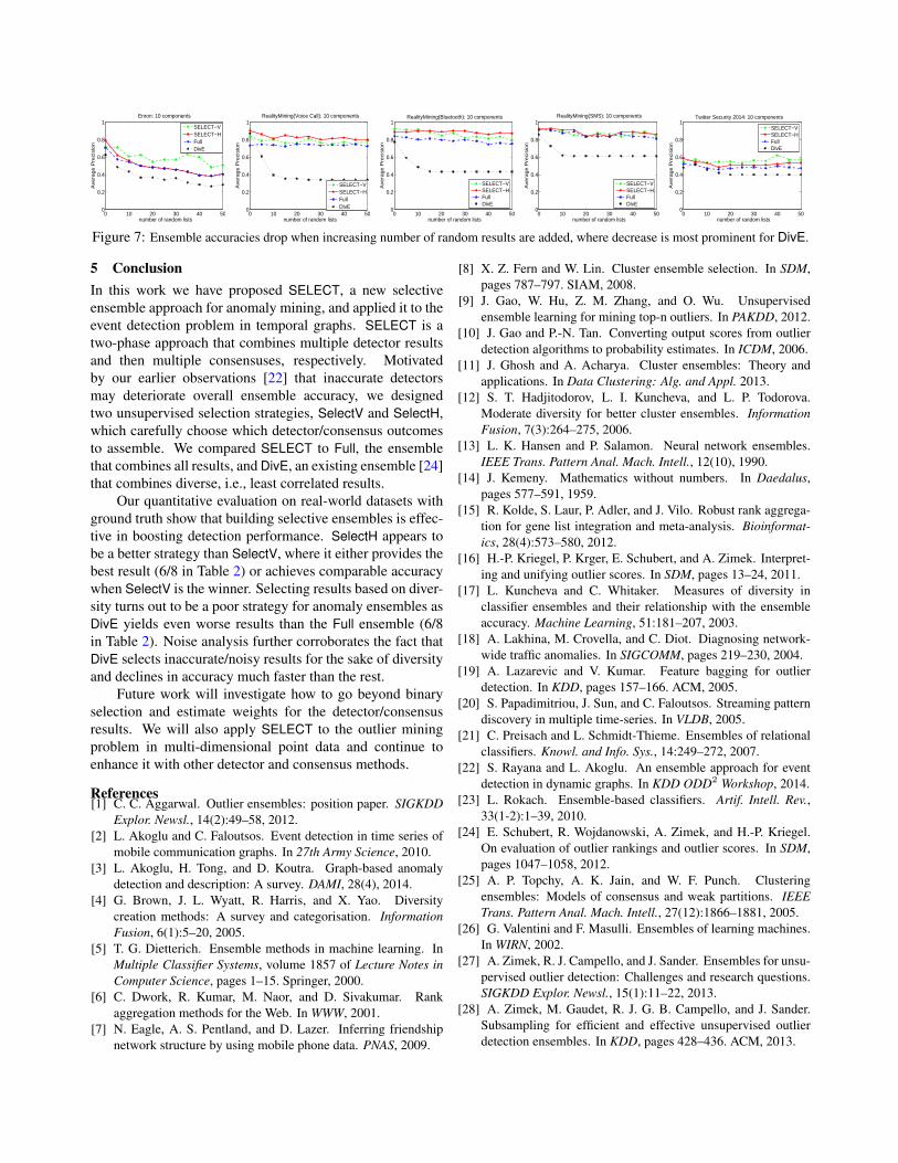
4.3 Noise Analysis Provided that selecting which resultsto combine would especially be beneficial in the presence ofinaccurate detectors, we design experiments where we intro-duce increasing number of noisy results into our ensembles.In particular, we create noisy results by randomly shufflingthe rank lists output by the base detectors and treat themas additional detector results. Figure 7 shows accuracies(avg.’ed over 10 independent runs) on all of our datasets for10 component ensembles (results using 20 components aresimilar, and provided in Figure 10 in Appendix B). We noticethat SELECT ensembles provide the most stable and effec-tive performance under increasing number of noisy results.More importantly, these results show that DivE degeneratesquite fast in the presence of noise, i.e., when the assumptionthat all results are reasonably accurate fails to hold.

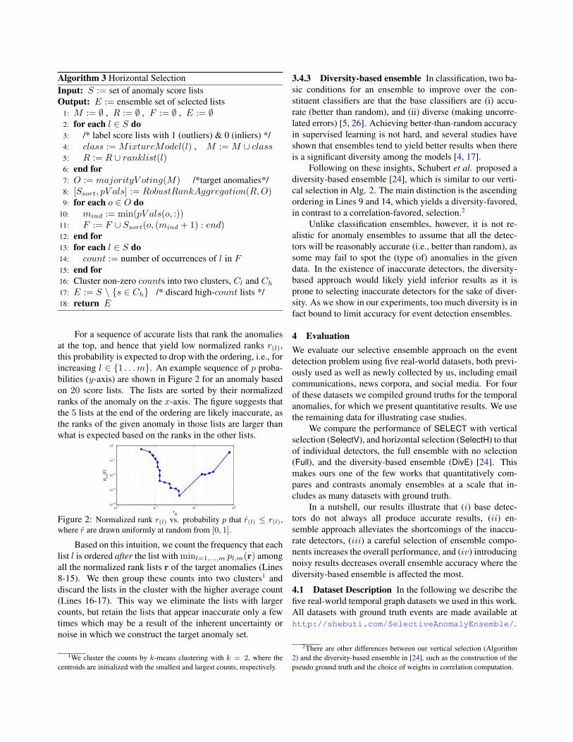
4.4 Case Studies In this section we evaluate our ensembleapproach qualitatively using the NYTNews corpus dataset,for which we do not have a compiled list of ground truthevents. Figure 8 shows the anomaly scores for the 2000-2007time line, provided by the five base detectors using weighteddegree feature (we have demonstrated a similar figure forEnronInc. in Figure 1 for additional qualitative analysis).

Top three events by SelectH are marked within boxes inthe figure, and corresponds to major events such as the 2001

elections, 9/11 WTC attacks, and the 2003 Columbia SpaceShuttle disaster. SelectH also ranks entities by associationto a detected event for attribution. We note that for theColumbia disaster, NASA and the seven astronauts killed inthe explosion rank at the top. The visualization of the changein Figure 9 shows that a heavy clique with high degree nodesemerges in the graph structure at the time of the event.

Eigen-behaviors

Probabilistic Approach

SPIRIT

Subspace method

Moving Average

Z-s

core

1 – n

orm

. (s

um

p-v

alu

e)

pro

ject

ion

Time tick

SP

E

Ag

gr.

Dif

f.

Sco

re

Columbia

disaster

9/11

attack

2001

election

Figure 8: Anomaly scores from five base detectors (rows) for NYTnews corpus. Top 3 events by the final ensemble are marked withgreen boxes. (red bars: top 20 anomalous time points per detector)

Husband,

Rick D. (Col)

Chawla,

Kalpana (Dr)

Clark, Laurel

Salton (Dr)

Brown,

David M (Capt)

Mccool,

William C (Cmdr)

Anderson, Michael

P (Lt Col)

Ramon,

Ilan (Col)

NASA

United States

New York City

Bush, George W (Pres)

Iraq

Husband,

Rick D. (Col)

Chawla,

Kalpana (Dr)

Clark, Laurel

Salton (Dr)

Brown,

David M (Capt)

Mccool,

William C (Cmdr)

Anderson, Michael

P (Lt Col)

Ramon,

Ilan (Col)

NASA

United States

New York City

Bush, George W (Pres)

Iraq

Time tick 161 Time tick 162

Figure 9: During 2003 Columbia disaster a clique of NASA andthe seven killed astronauts emerges from time tick 161 to 162.

0 10 20 30 40 500

0.2

0.4

0.6

0.8

1Enron: 10 components

Ave

rag

e P

reci

sio

n

SELECT−VSELECT−HFullDivE

number of random lists0 10 20 30 40 50

0

0.2

0.4

0.6

0.8

1

Ave

rag

e P

reci

sio

n


RealityMining(Voice Call): 10 components


0

0.2

0.4

0.6

0.8

1

Ave

rag

e P

reci

sio

n


number of random lists

RealityMining(Bluetooth): 10 components

0 10 20 30 40 500

0.2

0.4

0.6

0.8

1

Ave

rag

e P

reci

sio

n


RealityMining(SMS): 10 components


0

0.2

0.4

0.6

0.8

1

Ave

rag

e P

reci

sio

n



Twitter Security 2014: 10 components

Figure 7: Ensemble accuracies drop when increasing number of random results are added, where decrease is most prominent for DivE.

5 ConclusionIn this work we have proposed SELECT, a new selectiveensemble approach for anomaly mining, and applied it to theevent detection problem in temporal graphs. SELECT is atwo-phase approach that combines multiple detector resultsand then multiple consensuses, respectively. Motivatedby our earlier observations [22] that inaccurate detectorsmay deteriorate overall ensemble accuracy, we designedtwo unsupervised selection strategies, SelectV and SelectH,which carefully choose which detector/consensus outcomesto assemble. We compared SELECT to Full, the ensemblethat combines all results, and DivE, an existing ensemble [24]that combines diverse, i.e., least correlated results.

Our quantitative evaluation on real-world datasets withground truth show that building selective ensembles is effec-tive in boosting detection performance. SelectH appears tobe a better strategy than SelectV, where it either provides thebest result (6/8 in Table 2) or achieves comparable accuracywhen SelectV is the winner. Selecting results based on diver-sity turns out to be a poor strategy for anomaly ensembles asDivE yields even worse results than the Full ensemble (6/8in Table 2). Noise analysis further corroborates the fact thatDivE selects inaccurate/noisy results for the sake of diversityand declines in accuracy much faster than the rest.

Future work will investigate how to go beyond binaryselection and estimate weights for the detector/consensusresults. We will also apply SELECT to the outlier miningproblem in multi-dimensional point data and continue toenhance it with other detector and consensus methods.

References[1] C. C. Aggarwal. Outlier ensembles: position paper. SIGKDD

Explor. Newsl., 14(2):49–58, 2012.[2] L. Akoglu and C. Faloutsos. Event detection in time series of

mobile communication graphs. In 27th Army Science, 2010.[3] L. Akoglu, H. Tong, and D. Koutra. Graph-based anomaly

detection and description: A survey. DAMI, 28(4), 2014.[4] G. Brown, J. L. Wyatt, R. Harris, and X. Yao. Diversity

creation methods: A survey and categorisation. InformationFusion, 6(1):5–20, 2005.

[5] T. G. Dietterich. Ensemble methods in machine learning. InMultiple Classifier Systems, volume 1857 of Lecture Notes inComputer Science, pages 1–15. Springer, 2000.

[6] C. Dwork, R. Kumar, M. Naor, and D. Sivakumar. Rankaggregation methods for the Web. In WWW, 2001.

[7] N. Eagle, A. S. Pentland, and D. Lazer. Inferring friendshipnetwork structure by using mobile phone data. PNAS, 2009.

[8] X. Z. Fern and W. Lin. Cluster ensemble selection. In SDM,pages 787–797. SIAM, 2008.

[9] J. Gao, W. Hu, Z. M. Zhang, and O. Wu. Unsupervisedensemble learning for mining top-n outliers. In PAKDD, 2012.

[10] J. Gao and P.-N. Tan. Converting output scores from outlierdetection algorithms to probability estimates. In ICDM, 2006.

[11] J. Ghosh and A. Acharya. Cluster ensembles: Theory andapplications. In Data Clustering: Alg. and Appl. 2013.

[12] S. T. Hadjitodorov, L. I. Kuncheva, and L. P. Todorova.Moderate diversity for better cluster ensembles. InformationFusion, 7(3):264–275, 2006.

[13] L. K. Hansen and P. Salamon. Neural network ensembles.IEEE Trans. Pattern Anal. Mach. Intell., 12(10), 1990.

[14] J. Kemeny. Mathematics without numbers. In Daedalus,pages 577–591, 1959.

[15] R. Kolde, S. Laur, P. Adler, and J. Vilo. Robust rank aggrega-tion for gene list integration and meta-analysis. Bioinformat-ics, 28(4):573–580, 2012.

[16] H.-P. Kriegel, P. Krger, E. Schubert, and A. Zimek. Interpret-ing and unifying outlier scores. In SDM, pages 13–24, 2011.

[17] L. Kuncheva and C. Whitaker. Measures of diversity inclassifier ensembles and their relationship with the ensembleaccuracy. Machine Learning, 51:181–207, 2003.

[18] A. Lakhina, M. Crovella, and C. Diot. Diagnosing network-wide traffic anomalies. In SIGCOMM, pages 219–230, 2004.

[19] A. Lazarevic and V. Kumar. Feature bagging for outlierdetection. In KDD, pages 157–166. ACM, 2005.

[20] S. Papadimitriou, J. Sun, and C. Faloutsos. Streaming patterndiscovery in multiple time-series. In VLDB, 2005.

[21] C. Preisach and L. Schmidt-Thieme. Ensembles of relationalclassifiers. Knowl. and Info. Sys., 14:249–272, 2007.

[22] S. Rayana and L. Akoglu. An ensemble approach for eventdetection in dynamic graphs. In KDD ODD2 Workshop, 2014.

[23] L. Rokach. Ensemble-based classifiers. Artif. Intell. Rev.,33(1-2):1–39, 2010.

[24] E. Schubert, R. Wojdanowski, A. Zimek, and H.-P. Kriegel.On evaluation of outlier rankings and outlier scores. In SDM,pages 1047–1058, 2012.

[25] A. P. Topchy, A. K. Jain, and W. F. Punch. Clusteringensembles: Models of consensus and weak partitions. IEEETrans. Pattern Anal. Mach. Intell., 27(12):1866–1881, 2005.

[26] G. Valentini and F. Masulli. Ensembles of learning machines.In WIRN, 2002.

[27] A. Zimek, R. J. Campello, and J. Sander. Ensembles for unsu-pervised outlier detection: Challenges and research questions.SIGKDD Explor. Newsl., 15(1):11–22, 2013.

[28] A. Zimek, M. Gaudet, R. J. G. B. Campello, and J. Sander.Subsampling for efficient and effective unsupervised outlierdetection ensembles. In KDD, pages 428–436. ACM, 2013.

AppendixA SELECT Base Algorithms for Event DetectionA.1 Eigen Behavior based Event Detection (EBED).The multi-variate time series contain the feature values ofeach node over time and can be represented as a n ×t data matrix, for n nodes and t time points. EBED[29] defines sliding time windows of length w over theseries and computes the principal left singular vector ofeach n × w matrix W . This vector is the same as theprincipal eigenvector of WWT and is always positive dueto the Perron-Frobenius theorem [34]. Each eigenvectoru(t) is treated as the “eigen-behavior” of the system duringtime window t, the entries of which are interpreted as the“activity” of each node.

To score the time points, EBED computes the similaritybetween eigen-behavior u(t) and a summary of past eigen-behaviors r(t), where r(t) is the arithmetic average of u(t′)’sfor t′ < t. The anomalousness score of time point t isthen Z = 1 − u(t)·r(t) ∈ [0, 1], where high value of Zindicates a change point. For each anomalous time point t̄,EBED performs attribution by computing the relative change|ui(t̄)−ri(t̄)|

ui(t̄)of each node i at t̄. The higher the relative

change, the more anomalous the node is.

A.2 Probabilistic Time Series Anomaly Detection (PT-SAD). A common approach to time series anomaly detec-tion is to probabilistically model a given series and detectanomalous time points based on their likelihood under themodel. PTSAD models each series with four different para-metric models and performs model selection to identify thebest fit for each series. Our first model is the Poisson, whichis used often for fitting count data. However, Poisson is notsufficient for sparse series with many zeros. Since real-worlddata is frequently characterized by over-dispersion and ex-cess number of zeros, we employ a second model calledZero-Inflated Poisson (ZIP) [32] to account for data sparsity.

We further look for simpler models which fit data withmany zeros and employ the Hurdle models [35]. Ratherthan using a single but complex distribution, Hurdle mod-els assume that the data is generated by two simple, sepa-rate processes; (i) the hurdle and (ii) the count processes.The hurdle process determines whether there exists activityat a given time point and in case of activity the count pro-cess determines the actual (positive) counts. For the hurdleprocess, we employ two different models. First is the inde-pendent Bernoulli and the second is the first order Markovmodel which better captures the dependencies, where anactivity influences the probability of subsequent activities.For the count process, we use the Zero-Truncated Poisson(ZTP) [30].

Overall we model each time series with four differentmodels: Poisson, ZIP, Bernoulli+ZTP and Markov+ZTP. We

then employ Vuong’s likelihood ratio test [36] to select thebest model for individual series. Note that the best-fit modelfor each series may be different.

To score the time points, we perform a single-sided testto compute a p-value for each value x in a given series; i.e.,P (X ≥ x) = 1 − cdfH(x) + pdfH(x), where H is thebest-fit model for the series. The lower the p-value, themore anomalous the time point is. We then aggregate allthe p-values from all the series per time point by taking thenormalized sum of the p-values and inverting them to obtainscores ∈ [0, 1] (s.t. higher is more anomalous). For eachanomalous time point t̄, attribution is done by sorting thenodes (i.e., the series) based on their p-values at t̄.

A.3 Streaming Pattern DIscoveRy in multIple Time-Series (SPIRIT). SPIRIT [33] can incrementally capturecorrelations, discover trends, and dynamically detect changepoints in multi-variate time series. The main idea is to rep-resent the underlying trends of a large number of numericalstreams with a few hidden variables, where the hidden vari-ables are the projections of the observed streams onto theprincipal direction vectors (eigenvectors). These discoveredtrends are exploited for detecting change points in the series.

The algorithm starts with a specific number of hiddenvariables that capture the main trends of the data. When-ever the main trends change, new hidden variables are intro-duced or several of existing ones are discarded to capture thechange. SPIRIT can further quantify the change in the indi-vidual time series for attribution through their participationweights, which are the entries in the principal direction vec-tors. For further details on the algorithm, we refer the readerto the original paper by Papadimitriou et al. [33].

A.4 Anomalous Subspace based Event Detection(ASED). ASED [31] is based on the separation of high-dimensional space occupied by the time series into twodisjoint subspaces, the normal and the anomalous subspaces.Principal Component Analysis is used to separate the high-dimensional space, where the major principal componentscapture the most variance of the data and hence, constructthe normal subspace and the minor principal componentscapture the anomalous subspace. The projection of the timeseries data onto these two subspaces reflect the normal andanomalous behavior. To score the time points, ASED usesthe squared prediction error (SPE) of the residuals in theanomalous subspace. The residual values associated withindividual series at the anomalous time points are used tomeasure the anomalousness of nodes for attribution. For thespecifics of the algorithm, we refer to the original paper byLakhina et al. [31].

A.5 Moving Average based Event Detection (MAED).MAED is a simple approach that calculates the moving

average µt and the moving standard deviation σt of eachtime series corresponding to each node by extending the timewindow one point at a time. If the value at a specific timepoint is more than three moving standard deviations awayfrom the mean, then the point is considered as anomalousand assigned a non-zero score. The anomalousness score isthe difference between the original value and (µt + 3σt) at t.To score the time points collectively, MAED aggregates theirscores across all the series. For each anomalous time point t̄,attribution is done by sorting the nodes (i.e., the series) basedon the individual scores they assign to t̄.

B Additional Evaluation Results

Table 3: Accuracy of ensembles for EnronInc. (directed) (20components) (features: weighted in-/out-degree and unweighted in-/out-degree). ∗ depicts selected detector/consensus results.


Bas

eA

lgor

ithm

s

EBED (win) 0.1313 ∗ ∗PTSAD (win) 0.1462 ∗ ∗SPIRIT (win) 0.7032 ∗ ∗ASED (win) 0.5470 ∗ ∗ ∗MAED (win) 0.6670 ∗EBED (wout) 0.2846 ∗PTSAD (wout) 0.2118 ∗ ∗SPIRIT (wout) 0.4563 ∗ASED (wout) 0.0580 ∗MAED (wout) 0.7328 ∗ ∗EBED (uin) 0.0892 ∗PTSAD (uin) 0.1607 ∗ ∗SPIRIT (uin) 0.3996 ∗ ∗ASED (uin) 0.1395 ∗ ∗MAED (uin) 0.4439 ∗ ∗EBED (uout) 0.0225 ∗PTSAD (uout) 0.2546 ∗SPIRIT (uout) 0.1012 ∗ ∗ASED (uout) 0.0870 ∗MAED (uout) 0.4181 ∗

Con

sens

us

Inverse Rank ∗ 0.7121 ∗ 0.5660 0.6577 ∗ 0.7496Kemeny-Young ∗ 0.3033 ∗ 0.2495 0.5361 ∗ 0.5066RRA ∗ 0.5948 ∗ 0.5348 0.4948 ∗ 0.5774Uni (avg) ∗ 0.4838 ∗ 0.4325 ∗ 0.6047 ∗ 0.5336Uni (max) ∗ 0.3020 ∗ 0.2242 0.6633 ∗ 0.4280MM (avg) ∗ 0.5673 ∗ 0.4662 0.6761 ∗ 0.7217MM (max) ∗ 0.0216 ∗ 0.0216 ∗ 0.5355 0.0222

Final Ensemble 0.5420 0.4697 0.7018 0.7798

Table 4: Accuracy of ensembles for RealityMining Voice Call(directed) (10 components) (features: weighted in-/out-degree).∗: selected detector/consensus results.


Bas

eA

lgor

ithm

s

EBED (win) 0.3508 ∗PTSAD (win) 0.6284 ∗SPIRIT (win) 0.8309 ∗ ∗ASED (win) 0.9437 ∗ ∗MAED (win) 0.8809 ∗ ∗EBED (wout) 0.4122 ∗PTSAD (wout) 0.6273 ∗SPIRIT (wout) 0.7346 ∗ ∗ASED (wout) 0.9500 ∗MAED (wout) 0.8758 ∗

Con

sens

us

Inverse Rank ∗ 0.7544 0.6169 0.8880 ∗ 0.8222Kemeny-Young ∗ 0.8221 ∗ 0.7708 0.8619 ∗ 0.9309RRA ∗ 0.8154 0.5936 0.8901 ∗ 0.9416Uni (avg) ∗ 0.7798 ∗ 0.6413 ∗ 0.8370 ∗ 0.9098Uni (max) ∗ 0.6704 0.5757 0.7786 ∗ 0.7833MM (avg) ∗ 0.9190 ∗ 0.9162 0.8835 ∗ 0.9183MM (max) ∗ 0.4380 ∗ 0.8934 0.7569 0.4380

Final Ensemble 0.7302 0.8724 0.8370 0.9045

Table 5: Accuracy of ensembles for RealityMining Voice Call(directed) (20 components) (features: weighted in-/out-degree andunweighted in-/out-degree) ∗: selected detector/consensus results.


Bas

eA

lgor

ithm

s

EBED (win) 0.3508 ∗PTSAD (win) 0.6284 ∗SPIRIT (win) 0.8309 ∗ ∗ASED (win) 0.9437 ∗ ∗MAED (win) 0.8809 ∗ ∗EBED (wout) 0.4122 ∗PTSAD (wout) 0.6273 ∗SPIRIT (wout) 0.7346 ∗ASED (wout) 0.9500 ∗MAED (wout) 0.8758 ∗EBED (uin) 0.4173PTSAD (uin) 0.8636 ∗ ∗SPIRIT (uin) 0.8313 ∗ASED (uin) 0.9191 ∗MAED (uin) 0.8706 ∗ ∗EBED (uout) 0.4800 ∗PTSAD (uout) 0.8665 ∗SPIRIT (uout) 0.7480 ∗ASED (uout) 0.9229 ∗ ∗MAED (uout) 0.9115 ∗

Con

sens

us

Inverse Rank ∗ 0.8035 0.7952 0.9240 ∗ 0.8681Kemeny-Young ∗ 0.9064 0.9018 0.9076 ∗ 0.9158RRA ∗ 0.8866 ∗ 0.7771 0.9013 ∗ 0.9311Uni (avg) ∗ 0.8598 0.9192 ∗ 0.8448 ∗ 0.9102Uni (max) ∗ 0.6844 ∗ 0.6863 0.8517 ∗ 0.7611MM (avg) ∗ 0.9321 ∗ 0.9083 ∗ 0.8312 ∗ 0.9134MM (max) ∗ 0.4380 ∗ 0.8858 0.8015 0.4380

Final Ensemble 0.8011 0.8335 0.8847 0.8949

Table 6: Accuracy of ensembles for RealityMining Bluetooth(undirected) (10 components) (feature: weighted and unweighteddegree). ∗: selected detector/consensus results.


Bas

eA

lgor

ithm

s

EBED (wdeg) 0.4363 ∗PTSAD (wdeg) 0.5820 ∗ ∗SPIRIT (wdeg) 0.9499 ∗ ∗ASED (wdeg) 0.8601 ∗ ∗MAED (wdeg) 0.8359 ∗ ∗EBED (udeg) 0.4966 ∗PTSAD (udeg) 0.8694 ∗ ∗SPIRIT (udeg) 0.9162 ∗ ∗ASED (udeg) 0.7662 ∗ ∗MAED (udeg) 0.8788 ∗ ∗

Con

sens

us

Inverse Rank ∗ 0.8646 ∗ 0.8255 0.8790 ∗ 0.8538Kemeny-Young ∗ 0.9534 0.9169 0.9698 ∗ 0.9361RRA ∗ 0.9413 0.8318 0.9693 ∗ 0.9684Uni (avg) ∗ 0.9071 0.8654 ∗ 0.9193 ∗ 0.9225Uni (max) ∗ 0.6973 ∗ 0.6122 0.8270 ∗ 0.7126MM (avg) ∗ 0.9407 ∗ 0.9340 0.8596 ∗ 0.8892MM (max) ∗ 0.6461 ∗ 0.6374 0.8830 0.6461

Final Ensemble 0.8398 0.7735 0.9193 0.8886

Table 7: Accuracy of ensembles for RealityMining SMS (directed)(10 components) (features: weighted in-/out-degree). ∗: selecteddetector/consensus results.


Bas

eA

lgor

ithm

s

EBED (win) 0.6117 ∗PTSAD (win) 0.7003 ∗SPIRIT (win) 0.9256 ∗ ∗ASED (win) 0.6338 ∗ ∗MAED (win) 0.9002 ∗ ∗EBED (wout) 0.5595 ∗PTSAD (wout) 0.7023 ∗ ∗SPIRIT (wout) 0.8656 ∗ ∗ASED (wout) 0.9102 ∗ ∗MAED (wout) 0.9259 ∗ ∗

Con

sens

us

Inverse Rank ∗ 0.8309 0.8174 0.8933 ∗ 0.8044Kemeny-Young ∗ 0.9491 ∗ 0.8779 0.9511 ∗ 0.9386RRA ∗ 0.8761 ∗ 0.8424 0.9578 ∗ 0.9516Uni (avg) ∗ 0.8531 0.8247 ∗ 0.9283 ∗ 0.8684Uni (max) ∗ 0.8205 ∗ 0.7632 0.8829 ∗ 0.8678MM (avg) ∗ 0.9276 ∗ 0.9487 0.9492 ∗ 0.9084MM (max) ∗ 0.8907 ∗ 0.8577 0.9410 0.9011

Final Ensemble 0.9092 0.8598 0.9283 0.9217

Table 8: Accuracy of ensembles for RealityMining SMS (di-rected) (20 components) (features: weighted in-/out-degree and un-weighted in-/out-degree). ∗: selected detector/consensus results.


Bas

eA

lgor

ithm

s

EBED (win) 0.6117 ∗ ∗PTSAD (win) 0.7003 ∗SPIRIT (win) 0.9256 ∗ASED (win) 0.6338 ∗ ∗MAED (win) 0.9002 ∗EBED (wout) 0.5595 ∗PTSAD (wout) 0.7023SPIRIT (wout) 0.8656 ∗ASED (wout) 0.9102 ∗MAED (wout) 0.9259 ∗ ∗EBED (uin) 0.4407 ∗PTSAD (uin) 0.7809 ∗ ∗SPIRIT (uin) 0.7841 ∗ASED (uin) 0.6248 ∗ ∗MAED (uin) 0.8297 ∗ ∗EBED (uout) 0.3246PTSAD (uout) 0.9157 ∗ ∗SPIRIT (uout) 0.8744 ∗ASED (uout) 0.9150 ∗MAED (uout) 0.8005 ∗

Con

sens

us

Inverse Rank ∗ 0.9135 0.6751 0.9634 ∗ 0.9230Kemeny-Young ∗ 0.9286 ∗ 0.7567 0.9094 ∗ 0.9325RRA ∗ 0.9568 0.6465 0.9418 ∗ 0.9583Uni (avg) ∗ 0.8791 0.6499 ∗ 0.9294 ∗ 0.9156Uni (max) ∗ 0.7173 ∗ 0.6696 0.9342 0.8650MM (avg) ∗ 0.9107 ∗ 0.8942 0.8519 ∗ 0.9138MM (max) ∗ 0.8895 ∗ 0.8480 0.9307 0.8895

Final Ensemble 0.9542 0.8749 0.9294 0.9621

Table 9: Accuracy of ensembles for TwitterSecurity (undirected)(10 components) (features: weighted and unweighted degree). ∗:selected detector/consensus results.


Bas

eA

lgor

ithm

s

EBED (wdeg) 0.4000 ∗ ∗PTSAD (wdeg) 0.5400 ∗ ∗SPIRIT (wdeg) 0.4467 ∗ ∗ ∗ASED (wdeg) 0.6200 ∗ ∗ ∗MAED (wdeg) 0.4933 ∗EBED (udeg) 0.4133 ∗ ∗ ∗PTSAD (udeg) 0.5467 ∗ ∗SPIRIT (udeg) 0.3867 ∗ ∗ASED (udeg) 0.5400 ∗ ∗MAED (udeg) 0.4533 ∗

Con

sens

us

Inverse Rank ∗ 0.4467 0.4267 0.5133 ∗ 0.4667Kemeny-Young ∗ 0.5667 0.5333 0.5333 0.5800RRA ∗ 0.5867 ∗ 0.5333 0.5467 ∗ 0.5933Uni (avg) ∗ 0.5600 0.5000 ∗ 0.5467 ∗ 0.6000Uni (max) ∗ 0.4533 ∗ 0.4400 0.5800 0.4533MM (avg) ∗ 0.5333 ∗ 0.5667 0.5267 0.5600MM (max) ∗ 0.3667 ∗ 0.3667 0.5533 0.5733

Final Ensemble 0.5200 0.4800 0.5467 0.5867

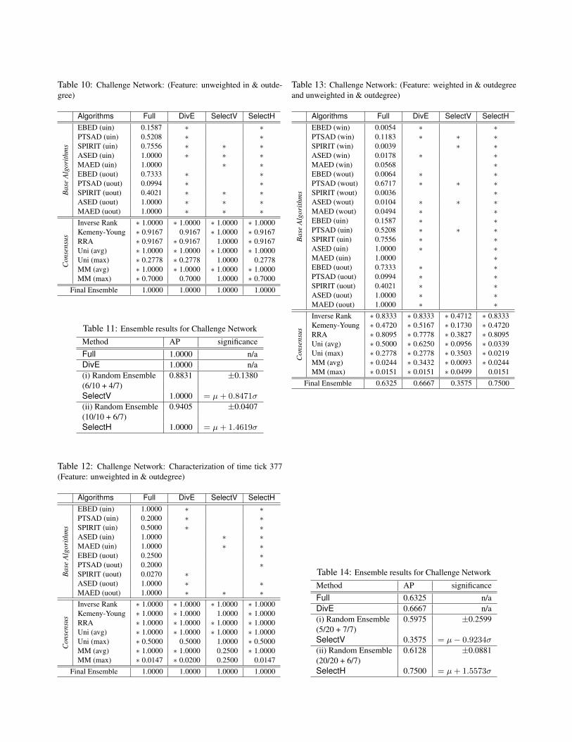
Table 10: Challenge Network: (Feature: unweighted in & outde-gree)

Algorithms Full DivE SelectV SelectH

Bas

eA

lgor

ithm

s

EBED (uin) 0.1587 ∗ ∗PTSAD (uin) 0.5208 ∗ ∗SPIRIT (uin) 0.7556 ∗ ∗ ∗ASED (uin) 1.0000 ∗ ∗ ∗MAED (uin) 1.0000 ∗ ∗EBED (uout) 0.7333 ∗ ∗PTSAD (uout) 0.0994 ∗ ∗SPIRIT (uout) 0.4021 ∗ ∗ ∗ASED (uout) 1.0000 ∗ ∗ ∗MAED (uout) 1.0000 ∗ ∗ ∗

Con

sens

us

Inverse Rank ∗ 1.0000 ∗ 1.0000 ∗ 1.0000 ∗ 1.0000Kemeny-Young ∗ 0.9167 0.9167 ∗ 1.0000 ∗ 0.9167RRA ∗ 0.9167 ∗ 0.9167 1.0000 ∗ 0.9167Uni (avg) ∗ 1.0000 ∗ 1.0000 ∗ 1.0000 ∗ 1.0000Uni (max) ∗ 0.2778 ∗ 0.2778 1.0000 0.2778MM (avg) ∗ 1.0000 ∗ 1.0000 ∗ 1.0000 ∗ 1.0000MM (max) ∗ 0.7000 0.7000 1.0000 ∗ 0.7000

Final Ensemble 1.0000 1.0000 1.0000 1.0000

Table 11: Ensemble results for Challenge Network

Method AP significanceFull 1.0000 n/aDivE 1.0000 n/a(i) Random Ensemble 0.8831 ±0.1380(6/10 + 4/7)SelectV 1.0000 = µ+ 0.8471σ

(ii) Random Ensemble 0.9405 ±0.0407(10/10 + 6/7)SelectH 1.0000 = µ+ 1.4619σ

Table 12: Challenge Network: Characterization of time tick 377(Feature: unweighted in & outdegree)


Bas

eA

lgor

ithm

s

EBED (uin) 1.0000 ∗ ∗PTSAD (uin) 0.2000 ∗ ∗SPIRIT (uin) 0.5000 ∗ ∗ASED (uin) 1.0000 ∗ ∗MAED (uin) 1.0000 ∗ ∗EBED (uout) 0.2500 ∗PTSAD (uout) 0.2000 ∗SPIRIT (uout) 0.0270 ∗ASED (uout) 1.0000 ∗ ∗MAED (uout) 1.0000 ∗ ∗ ∗

Con

sens

us

Inverse Rank ∗ 1.0000 ∗ 1.0000 ∗ 1.0000 ∗ 1.0000Kemeny-Young ∗ 1.0000 ∗ 1.0000 1.0000 ∗ 1.0000RRA ∗ 1.0000 ∗ 1.0000 ∗ 1.0000 ∗ 1.0000Uni (avg) ∗ 1.0000 ∗ 1.0000 ∗ 1.0000 ∗ 1.0000Uni (max) ∗ 0.5000 0.5000 1.0000 ∗ 0.5000MM (avg) ∗ 1.0000 ∗ 1.0000 0.2500 ∗ 1.0000MM (max) ∗ 0.0147 ∗ 0.0200 0.2500 0.0147

Final Ensemble 1.0000 1.0000 1.0000 1.0000

Table 13: Challenge Network: (Feature: weighted in & outdegreeand unweighted in & outdegree)


Bas

eA

lgor

ithm

s

EBED (win) 0.0054 ∗ ∗PTSAD (win) 0.1183 ∗ ∗ ∗SPIRIT (win) 0.0039 ∗ ∗ASED (win) 0.0178 ∗ ∗MAED (win) 0.0568 ∗EBED (wout) 0.0064 ∗ ∗PTSAD (wout) 0.6717 ∗ ∗ ∗SPIRIT (wout) 0.0036 ∗ASED (wout) 0.0104 ∗ ∗ ∗MAED (wout) 0.0494 ∗ ∗EBED (uin) 0.1587 ∗ ∗PTSAD (uin) 0.5208 ∗ ∗ ∗SPIRIT (uin) 0.7556 ∗ ∗ASED (uin) 1.0000 ∗ ∗MAED (uin) 1.0000 ∗EBED (uout) 0.7333 ∗ ∗PTSAD (uout) 0.0994 ∗ ∗SPIRIT (uout) 0.4021 ∗ ∗ASED (uout) 1.0000 ∗ ∗MAED (uout) 1.0000 ∗ ∗

Con

sens

us

Inverse Rank ∗ 0.8333 ∗ 0.8333 ∗ 0.4712 ∗ 0.8333Kemeny-Young ∗ 0.4720 ∗ 0.5167 ∗ 0.1730 ∗ 0.4720RRA ∗ 0.8095 ∗ 0.7778 ∗ 0.3827 ∗ 0.8095Uni (avg) ∗ 0.5000 ∗ 0.6250 ∗ 0.0956 ∗ 0.0339Uni (max) ∗ 0.2778 ∗ 0.2778 ∗ 0.3503 ∗ 0.0219MM (avg) ∗ 0.0244 ∗ 0.3432 ∗ 0.0093 ∗ 0.0244MM (max) ∗ 0.0151 ∗ 0.0151 ∗ 0.0499 0.0151

Final Ensemble 0.6325 0.6667 0.3575 0.7500

Table 14: Ensemble results for Challenge Network

Method AP significanceFull 0.6325 n/aDivE 0.6667 n/a(i) Random Ensemble 0.5975 ±0.2599(5/20 + 7/7)SelectV 0.3575 = µ− 0.9234σ

(ii) Random Ensemble 0.6128 ±0.0881(20/20 + 6/7)SelectH 0.7500 = µ+ 1.5573σ

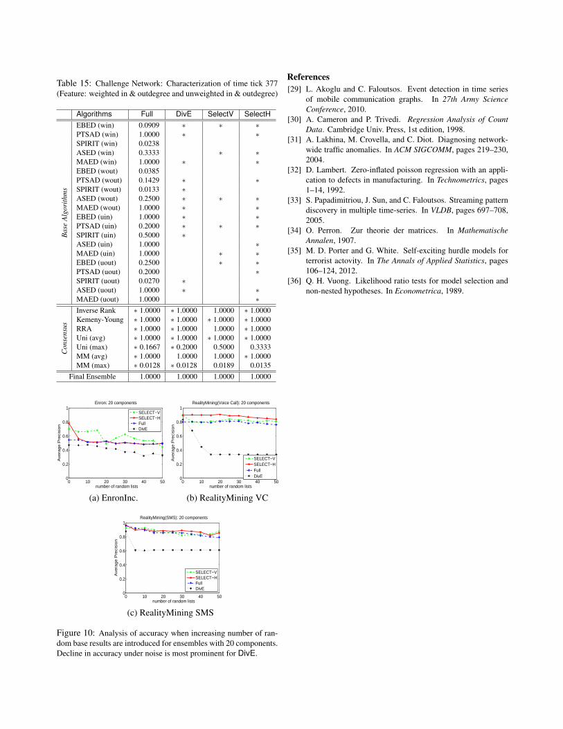
Table 15: Challenge Network: Characterization of time tick 377(Feature: weighted in & outdegree and unweighted in & outdegree)


Bas

eA

lgor

ithm

s

EBED (win) 0.0909 ∗ ∗ ∗PTSAD (win) 1.0000 ∗ ∗SPIRIT (win) 0.0238ASED (win) 0.3333 ∗ ∗MAED (win) 1.0000 ∗ ∗EBED (wout) 0.0385PTSAD (wout) 0.1429 ∗ ∗SPIRIT (wout) 0.0133 ∗ASED (wout) 0.2500 ∗ ∗ ∗MAED (wout) 1.0000 ∗ ∗EBED (uin) 1.0000 ∗ ∗PTSAD (uin) 0.2000 ∗ ∗ ∗SPIRIT (uin) 0.5000 ∗ASED (uin) 1.0000 ∗MAED (uin) 1.0000 ∗ ∗EBED (uout) 0.2500 ∗ ∗PTSAD (uout) 0.2000 ∗SPIRIT (uout) 0.0270 ∗ASED (uout) 1.0000 ∗ ∗MAED (uout) 1.0000 ∗

Con

sens

us

Inverse Rank ∗ 1.0000 ∗ 1.0000 1.0000 ∗ 1.0000Kemeny-Young ∗ 1.0000 ∗ 1.0000 ∗ 1.0000 ∗ 1.0000RRA ∗ 1.0000 ∗ 1.0000 1.0000 ∗ 1.0000Uni (avg) ∗ 1.0000 ∗ 1.0000 ∗ 1.0000 ∗ 1.0000Uni (max) ∗ 0.1667 ∗ 0.2000 0.5000 0.3333MM (avg) ∗ 1.0000 1.0000 1.0000 ∗ 1.0000MM (max) ∗ 0.0128 ∗ 0.0128 0.0189 0.0135

Final Ensemble 1.0000 1.0000 1.0000 1.0000

0 10 20 30 40 500

0.2

0.4

0.6

0.8

1Enron: 20 components

Ave

rag

e P

reci

sio

n



0

0.2

0.4

0.6

0.8

1

Ave

rag

e P

reci

sio

n


RealityMining(Voice Call): 20 components


(a) EnronInc. (b) RealityMining VC

0 10 20 30 40 500

0.2

0.4

0.6

0.8

1

Ave

rag

e P

reci

sio

n


RealityMining(SMS): 20 components


(c) RealityMining SMS

Figure 10: Analysis of accuracy when increasing number of ran-dom base results are introduced for ensembles with 20 components.Decline in accuracy under noise is most prominent for DivE.

References[29] L. Akoglu and C. Faloutsos. Event detection in time series

of mobile communication graphs. In 27th Army ScienceConference, 2010.

[30] A. Cameron and P. Trivedi. Regression Analysis of CountData. Cambridge Univ. Press, 1st edition, 1998.

[31] A. Lakhina, M. Crovella, and C. Diot. Diagnosing network-wide traffic anomalies. In ACM SIGCOMM, pages 219–230,2004.

[32] D. Lambert. Zero-inflated poisson regression with an appli-cation to defects in manufacturing. In Technometrics, pages1–14, 1992.

[33] S. Papadimitriou, J. Sun, and C. Faloutsos. Streaming patterndiscovery in multiple time-series. In VLDB, pages 697–708,2005.

[34] O. Perron. Zur theorie der matrices. In MathematischeAnnalen, 1907.

[35] M. D. Porter and G. White. Self-exciting hurdle models forterrorist actovity. In The Annals of Applied Statistics, pages106–124, 2012.

[36] Q. H. Vuong. Likelihood ratio tests for model selection andnon-nested hypotheses. In Econometrica, 1989.

less is more: building selective anomaly ensembles · less is more: building selective anomaly...

Documents