lerw as an example of off-critical sles
TRANSCRIPT

HAL Id: hal-00196372https://hal.archives-ouvertes.fr/hal-00196372
Submitted on 12 Dec 2007
HAL is a multi-disciplinary open accessarchive for the deposit and dissemination of sci-entific research documents, whether they are pub-lished or not. The documents may come fromteaching and research institutions in France orabroad, or from public or private research centers.
L’archive ouverte pluridisciplinaire HAL, estdestinée au dépôt et à la diffusion de documentsscientifiques de niveau recherche, publiés ou non,émanant des établissements d’enseignement et derecherche français ou étrangers, des laboratoirespublics ou privés.
LERW as an example of off-critical SLEsMichel Bauer, Denis Bernard, Kalle Kytola
To cite this version:Michel Bauer, Denis Bernard, Kalle Kytola. LERW as an example of off-critical SLEs. 45 pages, 2figures. 2007. <hal-00196372>

hal-
0019
6372
, ver
sion
2 -
12
Dec
200
7
LERW as an example of off-critical SLEs
Michel Bauer1, Denis Bernard2, Kalle Kytola3
Abstract
Two dimensional loop erased random walk (LERW) is a randomcurve, whose continuum limit is known to be a Schramm-Loewnerevolution (SLE) with parameter κ = 2. In this article we study “off-critical loop erased random walks”, loop erasures of random walkspenalized by their number of steps. On one hand we are able to iden-tify counterparts for some LERW observables in terms of symplecticfermions (c = −2), thus making further steps towards a field theo-retic description of LERWs. On the other hand, we show that it ispossible to understand the Loewner driving function of the continuumlimit of off-critical LERWs, thus providing an example of applicationof SLE-like techniques to models near their critical point. Such a de-scription is bound to be quite complicated because outside the criticalpoint one has a finite correlation length and therefore no conformalinvariance. However, the example here shows the question need notbe intractable. We will present the results with emphasis on generalfeatures that can be expected to be true in other off-critical models.
1Service de Physique Theorique de Saclay, CEA-Saclay, 91191 Gif-sur-Yvette, Franceand Laboratoire de Physique Theorique, Ecole Normale Superieure, 24 rue Lhomond,75005 Paris, France. <[email protected]>
2Member of the CNRS; Laboratoire de Physique Theorique, Ecole Normale Superieure,24 rue Lhomond, 75005 Paris, France. <[email protected]>
3Laboratoire de Physique Theorique et Modeles Statistiques, Universite Paris Sud,91405 Orsay, France and Service de Physique Theorique de Saclay, CEA-Saclay, 91191Gif-sur-Yvette, France. <[email protected]>
1

1 Introduction
Over the last few years, our understanding of interfaces in two dimensionalsystems at criticality has improved tremendously. Schramm’s idea [26] todescribe these interfaces via growth processes has met a great success. Weare now in position to answer quantitatively in a routine way many questionsof interest for physicists and/or mathematicians (the overlap is only partial,but non void).
All these successes suggest that we might try to be more ambitious andit seems that time has come to start thinking about what can be said forinterfaces in non-critical systems. So far, the only attempts in this directionseem to be [8, 25], although also some yet unpublished work [24] will treatquestions similar to this article in various models.
Needless to say, we do not aim to achieve general and definitive successin these notes. It is more our purpose to review some examples and seewhat we can say in each situation. We shall go a bit deeper into the specificexample of loop erased random walks (LERW). This choice has a numberof reasons. First, certain quantities for the LERW can be computed usingonly the underlying walk (with its loops kept), whose scaling limit is thefamiliar Brownian motion. This is the case for instance of boundary hittingprobabilities. Second, the quantum field theory of the LERW is that ofsymplectic fermions, a free fermionic theory. This relationship is part of thestandard lore at criticality, but it persists in the massive situation, and thespecific perturbation we study is related to the Brownian local time, makingit possible to compare closely the points of view of physics and mathematics.
To understand the difficulties inherent to the study of noncritical inter-faces, it is perhaps worth spending some time on the physical and mathe-matical views concerning criticality and conformal invariance
In statistical mechanics on the lattice, for generic values of the parameters(collectively called J here, examples include temperature, pressure, magneticfield, fugacity) the connected correlations among local observables decreasequickly (typically exponentially) with the distance : a correlation length n(J)(in lattice units) can be defined and turns out to be of the order of a finitenumber of lattice mesh. Achieving a large n(J) requires to adjust the pa-rameters. Imagine we cover the plane (or approximate a fixed domain inthe plane) with a lattice of mesh a, and tune the parameters J in such away that the macroscopic correlation length an(J) = ζ remains fixed while agoes to 0. Then it is expected on physical grounds that a limiting continuumtheory exists, which may describe only some of the initial degrees of freedomin the system. Lattice translation symmetry becomes usual translation in-variance in the limit. Rotation invariance is also very often restored. Over
2

scales s≫ a the discrete system is expected to be well approximated by thecontinuum theory.
In the limit a → 0, J tends to a limiting critical value Jc (when severalparameters are present this may be a critical manifold). The approach of Jto Jc when a → 0 is described by critical exponents. As n(Jc) is infinite,so is an(Jc) for any a, and the macroscopic correlation length is infinite atthe critical point as well : the system has no characteristic length scale andthe continuum limit is scale invariant. Over scales s≪ ζ the continuum off-critical system is expected to be well approximated by the critical system. Onthe lattice, an infinite number of control parameters can easily be exhibited,but if only their influence on the long distance physics is considered theequivalence classes form usually a finite dimensional space. Similarly, inthe continuum limit, usually only a finite number of perturbations out ofcriticality are relevant.
For many two dimensional systems of interest, translation, rotation andscale invariance give local conformal invariance for free : the descriptionsof the system in two conformally equivalent geometries are related by purekinematics. This remarkable feature that emerges only in the continuumlimit is suggested by convincing physical arguments but unproved in almostall cases of interest. The consequences of conformal invariance have beenvigorously exploited by physicists for local observables since the 1984 andthe seminal paper [7], even if the road to a complete classification of localtwo dimensional conformal field theories is still a distant horizon.
Schramm’s result in 1999 [26], on the other hand, is a complete clas-sification of probability measures on random curves in (simply connected)domains of the complex plane (say joining two boundary points for definite-ness) satisfying two axioms : conformal invariance and the domain Markovproperty. Again, the actual proof that a lattice interface has a limiting con-tinuum description which satisfies the two axioms requires independent hardwork. However the number of treated cases is growing rapidly, including theLERW, the Ising model, the harmonic navigator, percolation1. A notori-ous exception which up to now has resisted to all attacks is the case of selfavoiding walks.
Suppose that for each triple (D, x0, x∞) consisting of a domain with twomarked boundary points one has a probability measure on curves joining x0
to x∞ (so we have the chordal case in mind). Consider an initial segmentof curve, say γ, joining x0 to a bulk point x′ in D. The domain Markov
1But it should be noted that most of the proofs deal with a specific version on a specificlattice, which is rather unsatisfactory for a physicist thinking more in termes of universalityclasses.
3

property relates the distribution of random curves in two situations : itstates the equality of 1) the distribution of the rest of the random curve fromx′ to x∞ in D conditional on γ and 2) the distribution of the random curvefrom x′ to x∞ in D\γ.
This leads naturally to a description of the random curve as a growthprocess : if one knows how to grow an (infinitesimal) initial segment γ in(D, x0, x∞) from x0 to x∞, one can apply the domain Markov property tobuild the rest of the curve as a curve in the cut domain (D\γ, x′, x∞) and thenconformal invariance to ”unzip” the cut i.e. map (D\γ, x′, x∞) conformallyto (D, x0, x∞), so that another (infinitesimal) initial segment can be grownand mapped back to (D\γ, x′, x∞) to get a larger piece of curve, and so on.
Technically, Schramm’s proof is made simpler by using the upper halfplane H with 0 and ∞ as marked points, with a time parameterization ofthe curve by (half) its capacity. Then the conformal map gt(z) that unzipsthe curve grown up to time t and behaves at ∞ like z + O(z−1) satisfies
a Loewner differential equation dgt(z)dt
= 2gt(z)−ξt
which amounts to encodingthe growing curve via the real continuous driving function ξt. It should bestressed that this representation is valid for any curve (or more generallyany locally growing hull), independently of conformal invariance. However,the domain Markov property and conformal unzipping of the random curvesstraightforwardly translate into nice properties of the process ξt : it hasindependent and stationary increments. Continuity yields that ξt is a linearcombination of a Brownian motion and time. Finally scale invariance, theconformal transformations fixing (H, 0,∞), leaves the sole possibility thatξt =
√κBt for some normalized Brownian motion Bt and nonnegative scale
factor κ.Now suppose we consider the system out of criticality. Intuitively, there is
no doubt that the probability that the interface has a certain topology withrespect to a finite number of points in the domain should depend smoothly onthe correlation length ζ . But can we say a bit more ? Conformal invariancecannot be used to relate different domains and concentrating on the upperhalf plane case, as in the following, is really a choice2. We can then describethe interface again by a Loewner equation for a gζ
t (z) with some (off-critical)source ξζ
t . What do we expect for this new random process?At scales much smaller that the correlation length, i.e. in the ultraviolet
regime, the deviation from criticality is small, and for instance the inter-face should look locally just like the critical interface. This means that overshort time periods, the off-critical ξζ
t should not be much different from its
2Unless, as we will sometimes choose to do, we complicate matters by allowing theperturbation parameter (and thus correlation length) to vary from one point to another.
4

critical counterpart. Is is easily seen that if λ > 0, the rescaled Loewnermap 1
λgλ2t(λz) still satisfies the Loewner equation, but with a source 1
λξζλ2t.
Taking a small λ amounts to zoom at small scales near the origin and weexpect that (in some yet unspecified topology) limλ→0+
1λξζλ2t exists and is a√
κBt for some normalized Brownian motion. As the interface looks like acritical interface not only close to the origin but close to any of its points,we also expect that gζ
s maps the interface to a curve that looks like a crit-ical curve close to the origin, so that more generally for fixed s the limitlimλ→0+
1λ(ξζ
s+λ2t − ξζs ) should exist and be a
√κBt. Hence to each fixed s we
can in principle define a Brownian motion. The Brownian motions definedfor distinct s’s are moreover expected to be independent. To go further, wewould need to have some control on how uniform in s the convergence is,and how fast the correlations between 1
λ(ξζ
s+λ2t − ξζs ) for distinct values of
s decrease with λ. There could be some problem with inversions of limits.In the nice situation, we would naively deduce for the above facts that thequadratic variation of ξζ
t is exactly κt even at finite ζ . This raises the questionwhether ξζ
t can be represented as the sum of a Brownian motion (scaled by√κ) plus some process, contributing 0 to the quadratic variation, but whose
precise regularity would remain to be understood. Finally, the strongest re-lationship one could imagine between ξζ
t and its critical counterpart ξt wouldbe that their laws are mutually absolutely continuous over finite time inter-vals3. We shall see examples of this situation in the sequel, but at least onecounterexample is known, off-critical percolation [25]. On the lattice, the setof interfaces is discrete, and the question of absolute continuity trivializes.One can write down discrete martingales describing the relative weight of aninitial interface segment off/at criticality and a naive extrapolation to thecontinuum limit yields a candidate for the Radon-Nikodym derivative forthe growth of the interface. This is the basis of much of the forthcomingdiscussion.
At scales large with respect to ζ however, i.e. in the infrared regime, thebehavior is different and the interface should look like another SLE with anew κir. Think of the Ising model for example. At criticality κ = 3 butif the temperature is raised above the critical point, renormalization grouparguments indicate that at large scale the interface looks like the interfaceat infinite temperature, i.e; percolation and κir = 6. One expects in generalthat limλ→+∞
1λξζλ2t exists and is a
√κirBt. This means that the process ξζ
t
could yield information on the flow of the renormalization group. Whetherthis can be used as an effective tool is unclear at the moment.
3As a consequence, we may expect a Radon-Nikodym derivative for the interface atbest in finite domain but not in infinite domain such as the half plane.
5

Let us close this introduction with the following observations. Conformalinvariance and the domain Markov property have a rather different status.Whereas conformal invariance emerges (at best) in the continuum limit atcriticality, the domain Markov property makes sense and is satisfied on thelattice without tuning parameters for many systems of interest. It can be con-sidered as a manifestation of locality (in the physicists terminology). Hencethe domain Markov property is still expected to hold off criticality. Howeverthe consequences of this property on ξζ
t do not seem to have a simple formu-lation. As for conformal invariance, there is a trick to preserve it formallyout of the critical point : instead of perturbing with a scaling field O(z, z)times a coupling constant λ, perturb by a scaling field times a density λ(z, z)of appropriate weight, in such a way that λ(z, z)O(z, z)dz ∧ dz is a 2-form.This also gets rid of infrared divergences that occur in unbounded domainif λ(z, z) has compact support. We shall use this trick in some places, butbeware that if perturbation theory contains divergences, problems with scaleinvariance will arise, hence the cautious word ”formally” used above.
The paper is organized as follows. We start with a few examples in section2. A brief account of SLEs, as appropriate for our needs, is given in section3. Section 4 is devoted to the general philosophy of how one might hopeto attack the question of interfaces in off-critical models. In particular wepropose a field theoretical formula for Radon-Nikodym derivative betweenthe off-critical and critical measures on curves. The main example of LERWis treated in detail in section 5. We discuss the critical and off-critical fieldtheory for LERW, compute multipoint functions of the perturbing operatorand subinterval hitting probabilities — and derive in two ways the off-criticaldriving process to first order in the magnitude of the perturbation.
2 Examples
To give some concreteness to the thoughts presented in the introduction, wewill start with a couple of examples.
2.1 Self avoiding walks
Our first example deals with self avoiding walks (SAW). Consider a latticeof mesh size a embedded in a domain D in the complex plane. A sampleof a SAW is a simple nearest neighbor path on the lattice never visitingtwice any lattice site. The statistics of SAW is specified by giving the weightwγ = x|γ|, with |γ| the number of steps of γ and x the fugacity, to each path
6

γ. The partition function ZD is the sum ZD =∑
γ x|γ| and the probability of
occurrence of a curve γ is wγ/ZD.There is a critical value xc, depending on the lattice, for which typical
sample consists of paths of macroscopic sizes so that the continuum limita → 0 can be taken. This continuum limit is conjectured to be conformallyinvariant and described by chordal SLE8/3 if we restrict ourselves to SAWstarting and ending at prescribed points on the boundary of D.
The off-critical SAW model in the scaling regime consists of looking atSAW for fugacity x close to its critical value xc (and approaching xc in a ap-propriate way as the mesh size goes to zero). The continuous limiting theoryis not anymore conformally invariant as a scale parameter is introduced whenspecifying the way x approaches its critical value. Renormalization group ar-guments tell us that if x < xc the fugacity flows to zero at large distances sothat the partition function is dominated by the shortest path while if x > xc
it flows to the critical value corresponding to uniform spanning trees (UST)so that the partition function is dominated by these space filling paths.
The off-critical partition function∑
γ x|γ|c (x/xc)
|γ| can be written as anexpectation value with respect to the critical measure
ZD/ZcD
= E[ (x/xc)|γ| ]
with ZcD
the critical partition function and E the critical measure. If a samplepath γ has a typical length scale lD(γ), which is macroscopic in the criticaltheory, its number of steps scales as |γ| ≃ (lD(γ)/a)dκ with a the lattice meshsize and dκ the fractal dimension (more or less by definition of the fractaldimension). The scaling limit defining the continuous off-critical theory thenconsists of taking the limit x → xc such that ν := −a−dκ log(x/xc) is finiteas a → 0, that is (x − xc)/xc ≃ −ν adκ as a → 0. The parameter ν hasscaling dimension dκ and introduces a scale and a typical correlation lengthζ ≃ ν−1/dκ . This ensures that the relative weights (x/xc)
|γ| ≃ e−ν|γ|adκhave a
finite limit for typical paths as the mesh size goes to zero. In the continuumthe weights (relative the critical weights) are e−νLD(γ) with LD(γ) ≃ lD(γ)dκ
and the ratio of the off-critical partition function to the critical one is
ZD = E[ e−νLD(γ) ].
In the continuum limit the critical curve should be described by SLEsand we’d like to understand what the above teaches us about the off-criticalcurves. Recall that SLE comes as a one parameter family SLEκ, κ > 0, andthat critical SAW is conjectured to be described by SLE8/3. For simplicity weconsider here chordal SLE in which one looks for curves starting and endingat fixed points x0, x∞ on the boundary ∂D of D. Recall that in the SLE
7
construction the curves are given a ’time’ parametrization γ : [0, T ] → D,with γ0 = x0, γT = x∞, such that the filtration associated to the knowledge ofthe curve up to time t, (Fγ
t )t∈[0,T ], is the filtration generated by the Loewnerdriving process (ξt)t∈[0,T ], i.e. Fγ
t = σ{ξs : 0 ≤ s ≤ t} (for a reader not yetfamiliar with SLE, see section 3). The expectation E[· · · ] in the previousformula becomes the SLE measure. The mathematical definition of LD(·)is related to what is known as natural parametrization of the SLE curve[18, 21, 14]. It should satisfy the additivity property
LD(γ[0,t+s]) = LD(γ[0,t]) + LD\γ[0,t](γ[t,t+s]),
or even the stronger property that the natural parameterization of a pieceof SLE can be defined without reference to the domain, and L(γ[0,t+s]) =L(γ[0,t]) + L(γ[t,t+s]), since L(γ) is naively proportional to the number ofsteps of γ. We shall later define in a more general context the notion of aninterface energy and see that it possesses an analogous additivity property.
The factor e−νLD(·) specifies the Radon-Nikodym derivative of the off-critical measure with respect to the critical SLE measure so that the off-critical expectation of an observable O is
Eν [O ] = Z−1
DE[ e−νLD(·) O ] with ZD = E[ e−νLD(·) ].
If O is Fγt -measurable, that is if O only depends on the knowledge of the
curve up to time t, we have
Eν [O ] = E[Mt O ] with Mt := Z−1
DE[e−νLD(·)|Fγ
t ]
since E[ e−νLD(·) O] = E[ E[ e−νLD(·) O|Fγt ] ] = E[Mt O ] because we can take
out what is known, E[ e−νLD(·) O|Fγt ] = O E[ e−νLD(·)|Fγ
t ].In other words, the off-critical SLE (corresponding to the perturbation by
the natural parametrization) is obtained by weighting the SLE expectationwith Mt. As a conditional expected value, Mt is by construction a martingaleand M0 = 1 so that E
ν is correctly normalized to be a probability measure.Notice that, modulo a few regularity assumptions, this is the frameworkin which Girsanov’s theorem applies, as will be discussed in section 4.3.The additivity property of the natural parametrization implies that Mt =
e−νLD(γ[0,t]) Z−1D
E[e−νLD\γ[0,t]
(·)] so that
Mt = e−νLD(γ[0,t])ZD\γ[0,t]
ZD
. (1)
Mt can naturally be interpreted as the off-critical weight (relative to thecritical one) given to the curve γ[0,t]. It is made of two contributions, one is
8

a ratio of partition functions in the cut domain D \ γ[0,t] and in D, the otheris an ’interface energy’ contribution νLD(γ[0,t]) associated to the curve. Weshall recover this decomposition in a more general (but more formal) contextof perturbed SLEs in following sections.
2.2 Loop erased random walks
The second example deals with loop erased random walks (LERW) and itwill be further developed in section 5. Let us first recall the definition of aLERW. Again let us start with a lattice D(a) of mesh a embedded in a domainD. Given a path W = (W0,W1, · · · ,Wn) on the lattice its loop erasure γ isdefined as follows: let n0 = max{m : Wm = W0} and set γ0 = Wn0 = W0,next let n1 = max{m : Wm = Wn0+1} and set γ1 = Wn1 , and then inductivelylet nj+1 = max{m : Wm = Wnj+1} and set γj = Wnj
. This produces a simplepath γ = L(W ) = (γ0, γ1, . . . , γl) from γ0 = W0 to γl = Wn, called the loop-erasure of W , but its number of steps l is in general much smaller than thatof the original path W . We emphasize that the starting and end points arenot changed by the loop-erasing.
We point out that the above definition of loop erasure is equivalent tothe result of a recursive procedure of chronological loop erasing: the looperasure of a 0 step path (W0) is itself, γ = (W0) and if the erasure ofW = (W0, . . . ,Wm) is the simple path L(W ) = (γ0, . . . , γl) then for theloop erasure of W ′ = (W0, . . . ,Wm,Wm+1) there are two cases depending onwhether a loop is formed on step m+1. If Wm+1 /∈ {γ0, . . . , γl} then the looperasure of W ′ is γ′ = (γ0, . . . , γl,Wm+1). But if a loop is formed, Wm+1 = γk
for some k ≤ l (unique because γ is simple), then the loop erasure of W ′ isγ′ = (γ0, . . . , γk).
In this paper we shall be interested in paths starting at a boundary pointx0 and ending on a subset S of the boundary of D.
Statistics of LERW is defined by associating to any simple path γ a weightwγ =
∑
W :L(W )=γ µ|W |, where the sum is over all nearest neighbor paths W
whose erasures produce γ, and |W | denotes the number of steps of W . Thereis a critical value µc of the fugacity at which the underlying paths W becomejust ordinary random walks. The partition function
∑
γ wγ of LERWs fromz to S in D can be rewritten as a sum over walks in the domain D, startedfrom z and counting only those that exit the domain through set S
ZD;z;SRW =
∑
γ simple pathfrom z to S in D
wγ =∑
W walk fromz to S in D
µ|W | .
Written in terms of critical random walks, the partition function thus reads
9

EzRW
[
(µ/µc)|W | 1W
τRWD
∈S
]
, where τRWD
denotes the exit time of the random
walk W from D.Critical LERW corresponds to the critical fugacity and is described by
SLE2, see [26, 19, 31]. For µ < µc — which is the case we shall consider —paths of small lengths are more favourable and renormalization group argu-ments tell that at large distances the path of smallest length dominates. Theoff-critical theory in the scaling regime corresponds to non critical fugacityµ but approaching the critical one as the mesh size tends to zero. At fixedtypical macroscopic size, the number of steps of typical critical random walks(not of their loop erasures) scales as a−2, so that the scaling limit is such thatν := −a−2 log(µ/µc) is finite as a → 0, ie. (µ − µc)/µc ≃ −ν a2 and ν hasscaling dimension 2 and fixes a mass scale m ≃ √
ν and a correlation lengthζ ≃ 1/m. In this scaling limit the weights become (µ/µc)
|W | ≃ e−νa2|W | andthe random walks converge to two dimensional Brownian motions B witha2|W | = a2τRW
Dconverging to the times τD spent in D by B before exiting.
The off-critical partition function can thus be written as a Brownian expec-tation value ZD;z;S
ν −→ EzBM
[
e−ντD 1BτD∈S
]
as a ↓ 0. We may generalize thisby letting ν vary in space: steps out of site w ∈ D are given weight factorµ(w) = µc e
−a2ν(w) , in which case the partition function is
ZD;z;Sν = E
zRW
[
e−
∑
0≤j<τRWD
a2ν(Wj)1W
τRWD
∈S
]
−→a↓0
EzBM
[
e−∫ τD
0 ν(Bs) ds 1BτD∈S
]
.
The explicit weighting by e−ντRWD is transparent for the random walk, but
becomes less concrete for the LERW since the same path γ can be producedby random walks of different lengths and by walks that visit different points.Compared to the previous example of SAW, the description of the off-criticalLERW theory via SLE martingales is thus more involved but will (partially)be described in following sections.
2.3 Percolation
We will briefly also mention the case of off-critical percolation, just for somecomparisons. A way to study the scaling limit in the off-critical regime wassuggested in [8].
It is most convenient to define interfaces in percolation on the hexagonallattice. A configuration ω of face percolation on lattice domain D with latticespacing a is a colouring of all faces (hexagons) to open (1) or closed (0),i.e. ω ∈ {0, 1}FD, where FD is the set of faces. The Boltzmann weight ofa configuration is wω = p#open(ω)(1 − p)#closed(ω) — that is hexagons arechosen open with probability p independently. This hexagonal lattice face
10

percolation (triangular lattice site percolation) is critical at p = pc = 1/2and has been proven to be conformally invariant [28]. Exploration path, aninterface between closed and open clusters, is described in the continuumlimit by SLE6. Note also that
ZD =∑
ω
p#open(ω)(1 − p)#closed(ω) =∏
z∈FD
(p+ (1 − p)) = 1
for any p ∈ (0, 1).The off-critical regime now consists of changing the state of some faces
that are macroscopically pivotal, i.e. affect connectivity properties to macro-scopic distances. Informally, these faces are such that from their neighbor-hood there exists four paths of alternating colors to a macroscopic distanceaway from the point. The number of such points in the domain D should beof order |D| × a−3/4, so that in order to have finite probability of changing amacroscopically pivotal face we should take |p − pc| ∼ a3/4. We denote theperturbation amplitude by ν = a−3/4 log( p
pc).
For more about interfaces in off-critical percolation, the reader shouldturn to [8, 25]. The above remarks will be enough for us to give a point ofcomparison.
3 SLE basics
The method of Schramm-Loewner evolutions (SLE) is a significant recentdevelopment in the understanding of conformally invariant interfaces in twodimensions. We will describe the main ideas briefly and informally, and referthe reader to the many reviews of the topic, e.g. [17, 29, 12, 1, 11], amongwhich one can choose according to the desired level of mathematical rigour,physical intuition, emphasis and prerequisite knowledge.
3.1 Chordal SLE in the standard normalization
It was essentially shown in [26] that with assumptions of conformal invarianceand domain Markov property, probability measures on random curves in asimply connected domain D from a point x0 ∈ ∂D to x∞ ∈ ∂D are classifiedby one parameter, κ ≥ 0. These random curves are called chordal SLEκ.
The curves SLEκ are simple curves (no double points) iff 0 ≤ κ ≤ 4. Forthe purposes of this paper simple curves are enough, so we restrict ourselvesto this least complicated case. To describe the chordal SLEκ, we note thatby the assumed conformal invariance it suffices to discuss it in the domainH = {z ∈ C : ℑm z > 0} (upper half plane) from 0 to ∞ — for any
11

other choice of D, x0, x∞ one applies a conformal map f : H → D suchthat f(0) = x0, f(∞) = x∞. The existence of such f follows from Riemannmapping theorem and well-definedness of the resulting curve (f is only uniqueup to composition with a scaling z 7→ λz of H) from the scale invariance ofchordal SLE.
So, let 0 ≤ κ ≤ 4 and let gt(z) be the solution of the Loewner’s equation
d
dtgt(z) =
2
gt(z) − ξt(2)
with initial condition g0(z) = z ∈ H and ξt =√κBt a Brownian motion with
variance parameter κ. The solution exists up to time t for z ∈ H \ γ[0, t],where γ : [0,∞] → H is a random simple curve such that γ0 = 0 andγ∞ = ∞. This curve is called the (trace of) chordal SLEκ. Furthermore, gt
is the unique conformal map from H \ γ[0, t] to H with the hydrodynamicnormalization gt(z) = z + O(z−1) as z → ∞.
3.2 Chordal and dipolar SLEs in the half plane
The Loewner’s equation (2) can be used to describe any simple curve in H
starting from the boundary ∂H = R in the sense that gt is the hydrodynam-ically normalized conformal map from the complement of an initial segmentof the curve to the half plane. In particular, a chordal SLEκ in H from x0 ∈ R
to x∞ ∈ R is obtained by letting ξ0 = x0, η0 = x∞ and ξt, ηt solutions of theIto differential equations
{
dξt =√κ dBt + ρc
ξt−ηtdt
dηt = 2ηt−ξt
dt that is ηt = gt(x∞)
with ρc = κ − 6, see e.g. [27, 6]. The maximal time interval of the solutionis t ∈ [0, T ], where T is a (random) stopping time and γT = x∞.
Another interesting case is a curve in H depending on the starting pointx0 and two other points x+ < x− such that x0 /∈ [x+, x−]. If the two pointsplay a symmetric role, then the appropriate random conformally invariantcurve is the dipolar SLEκ [4]. We again have the Loewner’s equation (2) withξ0 = x0, X
±0 = x± and Ito differential equations
{
dξt =√κ dBt + ρd
ξt−X+t
dt+ ρd
ξt−X−t
dt
dX±t = 2
X±t −ξt
dt that is X±t = gt(x±)
with ρd = κ−62
. Again dipolar SLE is defined for t ∈ [0, T ], where T > 0 is(random) stopping time such that γT ∈ [x+, x−].
12

Both these examples can be understood from the point of view of sta-tistical physics in such a way that the (regularized) partition function forthe model in H is Z(x0, x∞) = |x∞ − x0|ρc/κ for the chordal SLEκ andZ(x0, x+, x−) = |x− − x0|ρd/κ |x+ − x0|ρd/κ |x− − x+|ρ
2d
/ 2κ for the dipolarSLEκ. The driving process satisfies dξt =
√κ dBt + κ(∂ξ logZ) dt and other
points follow the flow gt. For discussion of more general SLE variants of thiskind see [6, 15, 16, 1].
4 Probability measures
4.1 Definition from discrete stat. mech. models
Let us first recall how measures on curves are defined in statistical physicsmodels via Boltzmann weights. We have in mind Ising like models. Let Cbe the configuration space of a lattice statistical model defined on a domainD. For simplicity we assume C to be discrete and finite but as large asdesired. Let wc, wc ≥ 0, c ∈ C, be the Boltzmann weights and ZD thepartition function, ZD :=
∑
c∈C wc. By Boltzmann rules, the probability ofa configuration c is P[{c}] := wc/ZD, and this makes C a probability space.
In the present context, imagine that specific boundary conditions areimposed in such a way as to ensure the presence of an interface in D forany sample – for simplicity we consider only one interface. Given a curveγ in D, that we aim at identifying as an interface, there exists a subset ofconfigurations Cγ for which the actual interface coincides with the prescribedcurve γ. Again by Boltzmann rules, the probability of occurrence of thecurve γ as an interface, i.e. the probability of the event Cγ , is the ratio ofthe partition functions
PD[Cγ ] = ZD[γ]/ZD. (3)
where ZD[γ] is the conditioned partition function defined by the restrictedsum
ZD[γ] :=∑
c∈Cγ
wc .
The Boltzmann weights may depend on parameters such that for criticalvalues the statistical model is critical. We denote by P
0D
the probabilitymeasure at criticality, with Boltzmann weight w0, which in the continuumis expected to become an SLE measure if only the statistics of the interfaceare considered. We generically denote by P
νD
the off-critical measures, withBoltzmann weights wν . These probability measures differ by a density:
PνD
= MνD
P0D
13

where, by construction, MνD
are defined as ratio of partition functions (again,no degrees of freedom other than the shape of the interface are considered):
MνD
=Zν
D[γ]/Z0
D[γ]
ZνD/Z0
D
.
As in our previous examples, MνD
code for the off-critical weights relative tothe critical ones. On a finite lattice, they are typically well defined but theirexistence in the continuum limit may be questioned. This has to be analysedcase by case.
Assume as in the SLE context that the interfaces emerge from the bound-ary of D so that the cut domains D\γ are also domains of the complex plane.The restricted partition function ZD[γ] is then proportional to the partitionfunction in the cut domain
ZνD[γ] = eE
νD(γ)Zν
D\γ .
The extra term EνD(γ) arises from the energy of the lattice bonds which have
been cut from D to make D \ γ. We call it the ’interface energy’ of γ. Itinherits from the domain Markov property an additivity identity similar tothe one satisfied by the natural parameterization, i.e.
EνD(γ.γ′) = Eν
D(γ) + Eν
D\γ(γ′) .
where γ.γ′ is the concatenation of successive segments of the interface.The off-critical weights then read:
MνD(γ) = eE
νD(γ)−E0
D(γ)
ZνD\γ/Z
0D\γ
ZνD/Z0
D
. (4)
This can be compared with (1). The presence of the energy term EνD(γ) −
E0D(γ) in the continuum has also to be analysed case by case, see below. We
furthermore point out that there may be several natural choices of what toinclude in the Boltzmann weights and different choices may lead to differentEν
Dterm4 — to the extent that vanishing of this term can be a question of
convention.To make contact with SLE, we also define a stochastic growth process
that describes the curve, in terms of which we define a filtration on C. Con-sider portions of interfaces γ[0, t], where the index t specify say their lengths
4An easy example is the Ising model. Suppose we have boundary conditions suchthat spins on the boundary of the domain are fixed. Whether we include interactions ofthese fixed spins with each other in our Hamiltonian and therefore in ZD obviously has adramatic effect on the interface energy term while it doesn’t change the physics at all.
14

and will be identified with the ‘time’ of the process. We may partition ourconfiguration space according to these portions at time t. The elements ofthe partition Qt are denoted by Cγ[0,t]
, indexed by γ[0, t] in such a way thatc ∈ Cγ[0,t] if and only if the configuration c gives rise to γ[0, t] as a portionof the interface. Thus we have C =
⋃
γ[0,t] Cγ[0,t], with Cγ[0,t] all disjoint. Byconvention Q0 is the trivial partition with the whole configuration space Cas its single piece. We assume these partitions to be finer as t increasesbecause specifying longer and longer portions of interfaces defines finer andfiner partitions. This means that for any s > t and any element Cγ[0,t] ofthe partition at time t there exist elements of Qs which form a partition ofCγ[0,t] (corresponding to those γ[0, s] which extend γ[0, t]). To any partitionQt is associated a σ-algebra Fγ
t on C, the one generated by the elementsof this partition. Since these partitions are finer as ‘time’ t increases, theseconstitute a filtration (Fγ
t )t≥0 on C, i.e. Fγt ⊂ Fγ
s for s > t. The fact thatwe trivially get a filtration simply means that increasing ‘time’ t increasesthe knowledge on the system. In the SLE context the information aboutthe curve is encoded in the driving process (ξt)t≥0, so this filtration (Fγ
t )t≥0
becomes the one generated by ξ.On C with the filtration (Fγ
t )t≥0, we may define two processes using eitherthe critical P
0 or the off-critical Pν probability measures. They differ by
MνD(γ[0, t]) which can then be written as a conditioned expectation with
respect to the critical measure
MνD(γ[0, t]) =
Z0D
ZνD
E[wν
w0|Fγ
t ]
Thus MνD(γ[0, t]) is a P 0
D-martingale and the two processes differ by a mar-
tingale, which is the context in which Girsanov theorem applies. It is similarto what we encountered in the SAW example. One of our aims is to (try to)understand how this tautological construction applies in the continuum.
4.2 Continuum limit
4.2.1 Massive continuum limits in field theory
In the continuum limit, the critical model should be described by a con-formal field theory (CFT) and the critical measure on curves by SLE. TheBoltzmann weights are e−S with S the action. Off-critical perturbation isgenerated by a so-called perturbing field Φ so that
S = S0 + ν
∫
D
d2z Φ(z, z)
15

with S0 the conformal field theory action5. The ratio of the (off-critical) fieldtheory partition function to the CFT (critical) one is the expectation value
〈exp[−ν∫
Dd2zΦ(z, z)] (bdry cond.)〉D
〈(bdry cond.)〉D
(5)
where the brackets denote CFT expectations and the boundary conditions(bdry cond.) are implemented by insertion of appropriate boundary opera-tors, including in particular the operators that generate the interface.
The coupling constant ν has dimension 2 − h − h, linked to the scalingdimension h + h of the perturbing operator Φ. In our previous examples wedetermined explicitly this dimension by looking at the way the scaling limitis defined. We got (the perturbing operators in all cases are spinless, h = h):(i) SAW: ν has dimension dκ = 1 + κ/8, i.e. d8/3 = 4/3 for κ = 8/3 which isthe value corresponding to the SAW. The perturbing operator has dimensionhκ + hκ = 1 − κ/8, i.e. h = h = 1/3 for SAW. It is the operator Φ0;1
which is known to be the operator testing for the presence of the SLE curvein the neighbourhood of its point of insertion (in particular its one-pointfunction gives the probability for the SLE curve to visit a tiny neighbourhoodof a point in the complex plane, [3]). This had to be expected since theperturbation by the natural parametrization as described in the first sectionjust counts the number of lattice size boxes crossed by the curve.(ii) LERW: the coupling constant has dimension 2 so that the perturbingoperator has dimension h = h = 0 (up to logarithmic correction). We shallidentify it either in terms of symplectic fermions or in terms of Brownianlocal time in the following sections.(iii) Percolation: the coupling constant has dimension 3/4 and therefore theperturbing operator should have h = h = 5/8. This operator is the bulkfour-leg operator Φ0,2 testing for the presence of a macroscopically pivotalpoint.
4.2.2 Curves, RN-derivatives and interface energy
Assuming (with possibly a posteriori justifications) that the discrete martin-gale (4) has a nice continuum limit, one infers that the off-critical measureE
ν [ · · · ] and critical SLE measure E[ · · · ] on curves differ by a martingale (theRadon-Nikodym derivative exists) so that
Eν [X ] = E[Mν
t X ]5For simplicity we assume that there is only one coupling constant and thus only one
perturbing field. Furthermore, renormalization properties of the field theory expression ofthe partition functions would need to be analysed. We shall not dive into this problem inview of so (low and) formal level we are at.
16

for any Fγt -measurable observable with Mt given by the continuum limit of
eq.(4),
Mνt = e∆Eν
D(γ[0,t])
ZνD\γ[0,t]
/Z0D\γ[0,t]
ZνD/Z0
D
. (6)
We expect the above ratio of partition functions to become the field theoryexpression (5) in the continuum. This is clearly a complicated (and useless)formula, but the existence of Mν
t , at least in finite domain, is suggestedby the physical intuition that typical samples of the critical and off-criticalinterfaces look locally similar on scales small compared to the correlationlength which is macroscopic.
As far as we know, there is no simple field theoretical formula for thesurface energy term ∆Eν
D(γ[0,t]). However, to discuss whether this term is
present or not we may consider the discrete models and propose criteria.In the discrete setup we can typically write the offcritical Boltzmann
weight as wν = w0 e−∑
z ν(a)(z)φ(z), where φ is a field by which we perturbthe model. Under renormalization it corresponds to the scaling field Φin the sense that a−h−hφ(z) can in the limit a ↓ 0 be replaced by Φ(z).
With our choice ν(a)(z) = a2−h−hν(z), the sum∑
z∈D(a) ν(a)(z)φ(z) becomes∫
Dν(z)Φ(z, z)d2z in the continuum. The martingale Mt can be written in
terms of
ED(a)
[
exp(
−∑
z∈D(a)
ν(a)(z)φ(z))
∣
∣
∣Fγ
t
]
.
For example for SAW we have φ(z) = 1 if the walk passes through z andφ(z) = 0 otherwise. For the Ising model in near critical temperature, φ is theenergy, most conveniently defined on edges and not vertices, taking values±1.
Let us assume, having in mind spin models with local interactions orSAW, that φ(z) becomes determined (Fγ
t -measurable) for those z that aremicroscopically close to the curve γ(a)[0, t]. Moreover we must assume thedomain Markov property. We then get
M(a)t = const. × exp
(
−∑
z∈γ(a)[0,t]
a2−h−hν(z)φ(z))
× ED(a)\γ(a)[0,t]
[
exp(
∑
z∈D(a)\γ(a)[0,t]
a2−h−hν(z)φ(z))
]
.
The first part corresponds to the “interface energy” and the latter to the samemodel in the remaining domain. Since the number of points microscopically
17
close to the interface is of order ∼ a−d (where d is the fractal dimension of thecurve) and φ is typically bounded, the interface energy term should vanishin the continuum if 2−d−h−h > 0. In the case 2−d−h−h = 0 there mayremain a finite interface energy in the continuum. If 2− d− h− h < 0 someadditional cancellations would have to take place if the expressions were tohave continuum limits.
In view of the above, we notice that for example for percolation h = h =5/8 and d = 7/4, so we must be careful. Indeed, the near critical percolationinterfaces have been considered in [25] and they have been shown not to beabsolutely continuous with respect to the critical ones. The SAW is just themarginal case: h = h = 1/3 and d = 4/3 so that 2 − d − h − h = 0. Indeedwe expect a finite interface energy term LD(·) in the continuum.
However, the LERW doesn’t quite fit into the above setup as such —some long range interactions are present. The field φ(z) is now the numberof visits of the underlying walk to z, denoted by ℓ
D(a)(z) (for a more formal
definition, see section 5.1). It splits to ℓD(z) = ℓ(t)D
(z) + ℓD\γ[0,t](z) where theformer represents visits of the walk to z until the last time it comes to γt andthe latter represents the visits to z of the walk after this time. The quantityℓ(t)D
is not Fγt -measurable, but conditional on Fγ
t it is independent of the walkafter the last time it came to γt, see e.g. [19]. Thus we have
M(a)t = const. × E
[
exp(
− a2∑
z∈D(a)
ν(z)ℓ(t)
D(a)(z))∣
∣Fγt
]
× ED(a)\γ(a)[0,t]
[
exp(
a2∑
z∈D(a)\γ(a)[0,t]
ν(z)ℓD(a)\γ(a)[0,t](z)
)
]
.
The former term is again a property of the curve γ[0, t] and the domain: itcan be written in terms of random walk bubbles along the curve. The bubblesmay occasionally reach far away and thus they feel the values of ν in the wholedomain. In this sense an interface energy is present in the LERW (with ourconventions). The crucial difference is, however, that sites microscopicallyclose to the curve don’t contribute to the continuum limit. The values ofℓ(t)
D(a) on the curve remain of constant order (or diverges logarithmically still
in accordance with h = h = 0) while the number of sites close to the curveis ∼ a−d with d = 5/4. The contribution along the curve to the interfaceenergy thus vanishes like ∼ a3/4. We will use repeatedly the possibility tochange between domains D and D \ γ[0, t] in integrals of type
∫
ν(z)ℓ(z)d2z.
18

4.2.3 Field theoretic considerations of the RN-derivative
If it were correct to use the field theory expression (5) in formula (6) in thecontinuum limit without an interface energy term, we would have to firstorder in ν
Mνt = 1 + ν[
∫
D\γ[0,t]
d2z Nt(z) −∫
D
d2z N0(z) ] + · · · (7)
with
Nt(z) :=〈Φ(z, z) (bdry cond.)〉D\γ[0,t]
〈(bdry cond.)〉D\γ[0,t]
(8)
Here the (bdry cond.) refers to insertion of the appropriate boundary op-erators. For any point z, this ratio Nt(z) of correlation functions is a SLE(local) martingale, see e.g. [4, 6] and discussion in section 5.2.3. This is agood sign since Mt, if it exists, should be a martingale by construction. Inthe case of LERW, we will see also in section 5.2.3 that Nt(z) thus defined
is a sum of two parts, precisely corresponding to ℓD\γ[0,t] and ℓ(t)D
, and Nt(z)will indeed be closely related to the Radon-Nikodym derivative Mt.
4.3 Off-critical drift term and Girsanov theorem
As argued above, the off-critical expectations are related to the critical onesby insertion of the martingale Mν
t :
Eν [X ] = E[Mν
t X ]
for any Fγt -measurable observable. With some regularity assumptions, this is
a situation in which one may apply the Girsanov’s theorem, which relates thedecompositions of semimartingales in two probability measures one of whichis absolutely continuous with respect to the other. A simple illustration ofthe idea of Girsanov’s theorem is given in appendix A.
By definition of chordal SLE, ξt =√κBt with Bt a Brownian with respect
to the critical measure P0. Since Mt is a martingale, its Ito derivative is of
the form M−1t dMt = Vt dBt. Girsanov theorem tells us we may write
dξt =√κ dB′
t +√κVt dt
where B′t is Brownian motion with respect to the off-critical measure P
ν .In other words, weighting the expectation by the martingale Mt adds a
drift term to the stochastic evolution of the driving process ξt.
19

In the present context the martingale, if it exists, is given by (6) and itseems hopeless to compute and use the drift term directly. However, if thefield theoretic expression (7) is correct and we may omit contributions alongthe curve, we have to first order in perturbation simply
Vt dBt = ν
∫
D\γ[0,t]
d2z(
dNt(z))
.
In this situation we’d have under Pν the following drift, to first order in
perturbation ν
dξt ≈√κ dB′
t +√κν
∫
D
d2z(
d〈B,N〉t)
,
where 〈B,N〉t is the quadratic covariation of B and N , d〈B,N〉t = Vt dt. Insection 5.4 we will argue in two different ways that the above formula appliesto the LERW case. The explicit knowledge of Nt(z) will of course make thismore concrete.
The same change of drift applies to variants of SLE, where the drivingprocess contains a drift to start with. If a process has increments dξt =β dBt + α dt, it is only the random part of the increment β dBt that isaffected by the change of probability measure: the deterministic incrementsremain otherwise unchanged, but they gain the additional term discussedabove from the change of the random one.
5 Critical and off-critical LERW
In our attempt to gain insight to curves out of the critical point we nowconcentrate on the concrete example of loop-erased random walks (LERW). Itis worth noticing that the powerful method of Schramm-Loewner evolutions(SLE) that applies very generally to critical (conformally invariant) statisticalmechanics in two dimensions, was in fact first introduced with an applicationto LERW [26]. And one of the major early successes of SLEs was indeed theproof that scaling limit of (radial) LERW is (radial) SLE2 [19]. We will notconsider the radial LERW, but very natural variants of the same idea, namelychordal and dipolar LERW: in chordal setup the curves go from a boundarypoint x0 ∈ ∂D to another boundary point x∞ ∈ ∂D, and in the dipolar setupfrom a boundary point x0 to a boundary arch S ⊂ ∂D. Scaling limits of theseand other LERW variants at criticality have been studied mathematically in[31].
20
5.1 Continuum limit of LERWs
The discrete setting for LERWs was described in the introduction and wegave a formula for the offcritical measure in terms of the random walks: therelative weight was
e−
∑
0≤j≤τRWD
a2ν(Wj). (9)
There’s an alternative way of writing the Boltzmann weights of the walks onlattice D(a) of mesh a. Let ℓ(a)(z) = #{0 ≤ j < τRW
D(a) : W(a)j = z} be the
number of visits to z ∈ D(a) by the walk W (a). Then the Boltzmann weight
is
∏
0≤j<τ rw
D(a)
µ(a)(Wj) =∏
z∈D(a)
µ(a)(z)ℓ(z) .
In terms of the ν(z) = a−2 log(µc/µ(a)(z)) we can write the partition function
as an expected value for a random walk W (a) started from w(a) ∈ D(a)
ZD(a);w(a);S(a)
ν = Ew(a)
RW
[
exp(
−∑
z∈D(a)
a2ν(z)ℓ(a)(z))
1W
(a)
τRW
D(a)
∈S
]
. (10)
We will take the continuum limit by letting the lattice spacing a tendto zero and choosing D(a) that approximate a given open, simply connecteddomain D. The starting points w(a) approximate w ∈ D and the target setS(a) approximate S ⊂ ∂D. Simple random walksW (a) on the lattice should bescaled according to B
(a)t = W
(a)⌊t/a2⌋, so that B
(a)t converges to two-dimensional
Brownian motion Bt. In the limit a2∑
z∈D(a) becomes an integral∫
Dd2z and
the partition function (10) becomes
ZD;w;Sν = E
wBM
[
exp(
−∫
D
d2z ν(z)ℓ(z))
1BτD∈S
]
, (11)
where ℓ(z) needed no rescaling: it is the limit of ℓ(z(a)) with z(a) ∈ D(a)
approximating z ∈ D. This way ℓ(z) becomes the Brownian local time: ithas an interpretation as the occupation time density
∫ τD
0
F (Bt)dt =
∫
D
ℓ(z)F (z) d2z ,
a discete analogue of which we already used for F = ν to obtain the alterna-tive expression for the Boltzmann weights.
21

By comparing (11) with (5), we see that the Brownian local time ℓ(z),although not a CFT operator, plays a role very analogous to the perturbationΦ. Similarly, “1exit in S” together with “start from w” impose the boundaryconditions.
Remark: Our notation ℓ(z) is not totally fair, but in line with othertraditional field theory notation. It would be more appropriate to considerℓ as a random positive Borel measure on D with finite positive total massτD. This measure is supported on the graph B[0, τD) ⊂ D of the Brownianmotion, which has Lebesgue measure 0 (although its Hausdorff dimension is2). Therefore ℓ can not be absolutely continuous w.r.t. Lebesgue measure, asour notation suggests: we’d like ℓ(z) to be defined pointwise as the density ofthe occupation time ℓ with respect to Lebesgue measure. However, as usualin field theory, it is possible to make sense of pointwise correlation functionsas long as the insertions are not at coinciding points and we will stick tothe convenient notation ℓ(z) although it seems to misleadingly suggest apointwise definition of ℓ.
5.1.1 Continuum partition functions in the half-plane
We now choose as our domain the upper half plane H = {z ∈ C : ℑm z > 0}and as the target set an interval S = [x+, x−]. The partition function (11)can be written in terms of a Brownian expectation value
Zw;[x+,x−]ν = E
wBM
[
exp(
−∫ τH
0
ν(Bs) ds)
1BτH∈[x+,x−]
]
= EwBM
[
exp(
−∫
H
d2z ν(z)ℓ(z))
1BτH∈[x+,x−]
]
with τH = inf{t ≥ 0 : Bt /∈ H} the exit time from the half-plane.We would like to let the LERW start from the boundary, that is take
z → x0 ∈ ∂D. In the limit z → x0 the partition function vanishes likeZ
x0+iδ;[x+,x−]ν ∼ δ × (· · · ) so to obtain a nontrivial limit, we set
Zx0;[x+,x−]ν = lim
δ→0
1
δE
x0+iδBM
[
exp(
−∫ τH
0
ν(Bs)ds)
1BτH∈[x+,x−]
]
(12)
= limδ→0
1
δE
x0+iδBM
[
exp(
−∫
H
d2z ν(z)ℓ(z))
1BτH∈[x+,x−]
]
. (13)
Furthermore, we may wish to shrink the target set S = [x+, x−] to a pointx∞ so as to obtain a chordal LERW, nontrivial limit is obtained if we set
Zx0;x∞ν = lim
δ,δ′→0
1
δ δ′E
x0+iδBM
[
exp(
−∫ τH
0
ν(Bs)ds)
1BτH∈[x∞−δ′,x∞+δ′]
]
.
22

In the unperturbed case ν = 0, we have Zx0;[x+,x−]0 = 1
π
(
1x0−x−
− 1x0−x+
)
=1π
x−−x+
(x0−x−)(x0−x+)and Zx0;x∞
0 = 2π(x∞ − x0)
−2. The former is indeed the parti-tion function of a dipolar SLE2 and the latter is that of chordal SLE2 fromx0 to x∞, see [4, 6, 15, 16].
Partition functions with a nonzero perturbation will be considered in moredetail in section 5.4.1.
5.1.2 The perturbation and conformal transformations
The perturbation ℓ(z) corresponds to an operator of dimension zero. Accord-ing to a general argument that can be found e.g. in [10], this fact alreadymanifested itself when we observed that no rescaling under renormalizationwas needed in its continuum definition, a∆ℓ ℓ(a)(v(a)) → ℓ(z) with ∆ℓ = 0.From its definition as a local time of 2-d Brownian motion we can also di-rectly check how ℓ(z) transforms under conformal transformations. The localtime ℓ(z) gives us the occupation time in the following sense: if F : D → R,then
∫ τD
0
F (Bt) dt =
∫
D
F (z)ℓ(z) d2z .
Taking in place of F an approximate delta function, we see that ℓ(z) =∫ τD
0δ(Bt − z) dt.
Let f : D → D be conformal and (Bt)t∈[0,τD] Brownian motion in D startedfrom w ∈ D and stopped upon exiting the domain τD = inf{t ≥ 0 : Bt /∈ D}.Then a direct application of Ito’s formula tells us that (f(Bt))t∈[0,τD] is a
(two-component) martingale in D, started from w = f(w), and the quadraticvariation of its components is d〈F (B)j, F (B)k〉t = δj,k|f ′(Bt)|2 dt, (j, k =1, 2). The time changed process Bs = f(Bt(s)) with ds = |f ′(Bt)|2 dt is a
Brownian motion in D, started from w = f(w).Given F : D → R we set F = F ◦ f : D → R and we have by definitions
∫
D
F (z′)ℓD;w′(z
′) d2z′ =
∫ τD
0
F (Bs) ds
=
∫ τD
0
F (f(Bt))|f ′(Bt)|2 dt
=
∫
D
F (z)|f ′(z)|2ℓD;w(z) d2z
If F is an approximate delta function at z′ = f(z), then |f ′|2 × F is anapproximate delta at z and we conclude that ℓ indeed transforms as a scalar
ℓf(D);f(w)(f(z))in law= ℓD;w(z) .
23

We will later in section 5.2.2 identify the conformal field theory equivalentof ℓ(z) and exhibit its corresponding transformation properties.
5.1.3 Brownian local time expectations
The multipoint correlation functions of the perturbing operator ℓ(z) are thebasic building blocks of the perturbative analysis of LERW near critical pointsince we can expand the partition function (13) in powers of the small per-turbation ν = εν
Zx0;[x+,x−]εν = lim
δ→0
1
δE
x0+iδBM
[
e−ε∫
Hν(z)ℓ(z) d2z 1BτD
∈[x+,x−]
]
= Zx0;[x+,x−]0 +
∞∑
n=1
εn
n!
∫
···∫
d2z1· · ·d2zn ν(z1) · · · ν(zn)
×(
limδ→0
1
δE
x0+iδBM
[
ℓ(z1) · · · ℓ(zn) 1BτD∈[x+,x−]
])
. (14)
Next we will compute these explicitly and afterwards we’ll find the fieldtheoretic interpretation.
For a smooth compactly supported function f : D → R, let ℓf =∫ τD
0f(Bt) dt.
Consider the correlation function
CSf1,...,fn
(w) = EwBM
[(
n∏
j=1
ℓfj
)
1BτD∈S
]
.
If σ ≤ τD is a stopping time of the Brownian motion, then write ℓf =∫ σ
0f(Bt) dt +
∫ τD
σf(Bt) dt = ℓ≤σ
f + ℓ>σf . The part ℓ≤σ
f is FBMσ -measurable
while ℓ>σf depends on FBM
σ only through Bσ. Obviously we have ℓ≤0f = 0 and
dℓ≤t∧τD
f = 1t≤τDf(Bt) dt. By the strong Markov property we have
EwBM
[(
n∏
j=1
ℓfj
)
1BτD∈S
∣
∣
∣FBM
t∧τD
]
=∑
J⊂{1,...,n}
(
∏
j∈J
ℓ≤t∧τD
fj
)
× CS(fj)j∈∁J
(Bt∧τD)
and this is a martingale by construction. It is also a continuous semimartin-gale and its Ito drift
∑
J⊂{1,...,n}
{
∑
k∈J
1t≤τDfk(Bt)
(
∏
j∈J\{k}
ℓ≤t∧τD
fj
)
× CS(fj)j∈∁J
(Bt∧τD)
+(
∏
j∈J
ℓ≤t∧τD
fj
)
× 1
21t≤τD
△CS(fj)j∈∁J
(Bt∧τD)}
24

should vanish. At t = 0 we have simplifications due to ℓ≤0f = 0 and 10≤τD
= 1,
so this reduces to a useful differential equation for CSf1,...,fn
1
2△CS
f1,...,fn(w) +
n∑
k=1
fk(w)CS(fj)j 6=k
(w) = 0
in terms of correlation functions of type CSf1,...,fn−1
. Boundary conditionsfor n ≥ 1 are zero, and for n = 0 case the correlation function is just theharmonic measure of S, CS
∅ (w) = HD(w;S).We are interested in replacing fj(z) by δ(z− zj), in which case we denote
the correlation function by CS(w; z1, . . . , zn). It is then straightforward tosolve the recursion and the result is
CS(w; z1, . . . , zn) = EwBM
[
ℓ(z1) · · · ℓ(zn) 1BτD∈S
]
=∑
π∈Sn
GD(w, zπ(1))(
n∏
j=2
GD(zπ(j−1), zπ(j)))
HD(zπ(n), S) ,
where GD is the Green’s function △zGD(z, w) = −2δ(z − w) with Dirichletboundary conditions GD(z, w) → 0 as z → ∂D. To get the multipoint corre-lation function for Brownian motion conditioned to exit through S, we mustdivide by E
wBM[1BτD
∈S] = HD(w, S), which we remind is also the partitionfunction at criticality. The ratio has a nontrivial limit as we take w to theboundary of the domain. Alternatively, we can regularize both the correla-tion function and the partition function in the same manner, as suggestedalso by formula (14). In the half-plane H with S = [x+, x−], regularized asin section 5.1.1 we have
Cx0;[x+,x−](z1, . . . , zn)
:= limδ→0
1
δE
x0+iδBM
[
ℓ(z1) · · · ℓ(zn) 1BτD∈[x+,x−]
]
=∑
π∈Sn
KH(x0, zπ(1))(
n∏
j=2
GH(zπ(j−1), zπ(j)))
HH(zπ(n); [x+, x−]) , (15)
with explicit expressions
GH(z, w) = −1
πlog
∣
∣
z − w
z − w
∣
∣
KH(x0, z) = −2
πℑm
( 1
z − x0
)
HH(z, [x+, x−]) =1
πℑm
(
logz − x−z − x+
)
.
25

zπ(1)
zπ(2)· · ·
· · ·
zπ(n)
zπ(1)zπ(n)
· · ·
· · ·
zπ(2)
z
x
zz2
z1 S
GD(z1, z2) KD(x; z) HD(z;S)
x0 x∞x0 x+ x−
Figure 1: Example diagrams representing the terms in the local time multi-point correlation functions. Dipolar case (15) is on the left and chordal case(16) on the right.
It is convenient to represent the terms in this result diagrammatically as infigure 1. The chordal case is obtained by limit δ′ → 0 with choice x± =x∞ ∓ δ′,
Cx0;x∞(z1, . . . , zn)
:= limδ→0
1
δ δ′E
x0+iδBM
[
ℓ(z1) · · · ℓ(zn) 1BτD∈[x∞−δ′,x∞+δ′]
]
=∑
π∈Sn
KH(x0, zπ(1))(
n∏
j=2
GH(zπ(j−1), zπ(j)))
KH(x∞, zπ(n)) . (16)
5.2 On conformal field theory of LERWs
It is known from general arguments that SLEκ corresponds to conformalfield theory of central charge c = (6−κ)(3κ−8)
2κ, [2], so that LERWs should have
c = −2. But we can be more specific about the CFT appropriate for ourcase.
First of all, LERWs are “dual” to uniform spanning trees (UST) [30,26, 19], for which fermionic field theories have been given [9], see also [23].Indeed a field theory of free symplectic fermions would have central chargec = −2, [13]. The theory is Gaussian. It has two basic fields χ+ and χ−
26

whose correlation functions in domain D (Dirichlet boundary conditions) aredetermined by
〈χα(z, z)χβ(w,w)〉 = JαβGD(z, w) ,
with J++ = 0 = J−−, J+− = 1 = −J−+, and the Wick’s formula.The fields χα(z, z) are fermionic but scalars, meaning that they transform
like scalars under conformal transformations. We shall also be interested inthe composite operator :χ−χ+: which has to be defined via a point splittingto remove the short distance singularity
:χ− χ+: (z, z) = limz→w
χ−(z, z)χ+(w,w) − 1
2πlog |z − w|2
Due to this regularisation, :χ−χ+: transforms with a logarithmic anomalyunder conformal transformations:
:χ− χ+: (z, z) → :χ− χ+: (g(z), g(z)) − 1
2πlog |g′(z)|2 . (17)
The stress tensor is T (z) = 2π :∂zχ+(z, z) ∂zχ
−(z, z): with the normalordering defined by a point splitting similar as above. It is easy to verify thatboth operators ∂zχ
α are operators of dimension 1 satisfying the level two nullvector equation (L−2 − 1/2L2
−1)∂zχα = 0 with Ln, T (z) =
∑
n Lnz−n−2, the
Virasoro generators. It is this equation which helps identifying the symplec-tic fermions as the CFT associated to LERW. We will be able to identifysome other fields with natural LERW quantities, although there are someimportant ones for which a good understanding is still lacking (to us).
5.2.1 Boundary changing operators
The partition functions without perturbation involve only boundary opera-tors that account for the LERW starting from x0 ∈ R and aiming at S ⊂ R.We will identify them below.
We consider the symplectic fermion field theory in the upper half planeH. Let us define the boundary fields ψ± as normal derivatives of χ± on thereal axis
ψ±(x0) = limδ→0
1
δχ±(x0 + iδ, x0 − iδ) .
The level two null field equation says the fields ψ+ and ψ− can accountfor starting point and end point of SLE2 curves [2, 4, 6] (see also section5.2.3). And indeed, the two point function 〈ψ+(x0)ψ
−(x∞)〉 = 2π(x∞ −x0)
−2
27

reproduces our partition function in the chordal setup, compare with sections3 and 5.1.1.
Let us then remark that the dipolar LERW from x0 to [x+, x−], condi-tioned to hit a point x∞ ∈ [x+, x−] is just the chordal LERW from x0 tox∞ as follows directly from the definitions. It has been pointed out in [5]that κ = 2 is the only value for which the corresponding property holds fordipolar and chordal SLEκ.
Following the above remark, we decompose the dipolar probability mea-sure according to the endpoint x∞ ∈ [x+, x−]
P0x0,[x+,x−] =
∫ x−
x+
dx∞A(x∞)P0x0;x∞
,
where A is the probability density for LERW to end at x∞
A(x∞) = limδ,δ′↓0
12δ′
H(x0 + iδ; [x∞ − δ′, x∞ + δ′])
H(x0 + iδ); [x+, x−])=
12Zx0;x∞
Zx0;[x+,x−]0
=(x0 − x−)(x0 − x+)
(x− − x+)(x∞ − x0)2. (18)
As this is just a ratio of the correlation functions, we may say that the dipolarboundary changing operators are ψ+(x0) and 1
2
∫ x−
x+ψ−(x∞) dx∞. Indeed, the
partition function is reproduced by
〈ψ+(x0)(1
2
∫ x−
x+
ψ−(x∞) dx∞)
〉 =1
π
x− − x+
(x− − x0)(x+ − x0)= Z
x0;[x+,x−]0 .
5.2.2 Field theory representation of Brownian local time
In section 5.1.3 we derived the expressions (15) and (16) for Brownian localtime correlations. We recall that in the chordal case, the multipoint correla-tion function in the upper half plane is
Cx0;x∞(z1, . . . , zn)
=∑
π∈Sn
KH(x0, zπ(1))(
n∏
j=2
GH(zπ(j−1), zπ(j)))
KH(x∞, zπ(n)) .
The two point functions of symplectic fermions involve the same buildingblocks 〈χ+(z)χ−(w)〉 = GH(z, w) and 〈ψ+(x)χ−(z)〉 = 〈χ+(z)ψ−(x)〉 =KH(x; z). Thus the formula is clearly reminiscent of what Wick’s formulagives for correlations of the composite operator
:χ−χ+:D (z) = limz′,z′′→z
(
χ−(z′)χ+(z′′) −GD(z′, z′′))
, (19)
28
zπ(1)
zπ(2)
zπ(|J |)
zπr′(2)
zπr(|Jr|)
zπr(1)
· · ·· · ·
zπr′(1)
zπr(2)
x0 x∞
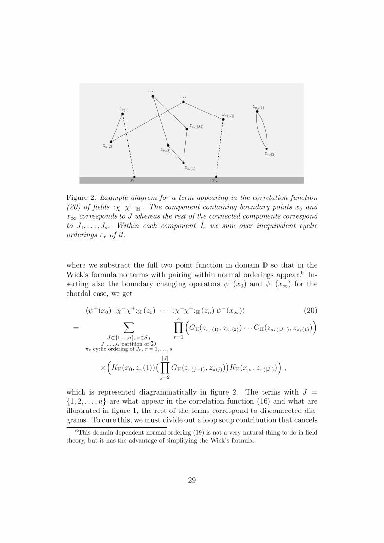
Figure 2: Example diagram for a term appearing in the correlation function(20) of fields :χ−χ+:H . The component containing boundary points x0 andx∞ corresponds to J whereas the rest of the connected components correspondto J1, . . . , Js. Within each component Jr we sum over inequivalent cyclicorderings πr of it.
where we substract the full two point function in domain D so that in theWick’s formula no terms with pairing within normal orderings appear.6 In-serting also the boundary changing operators ψ+(x0) and ψ−(x∞) for thechordal case, we get
〈ψ+(x0) :χ−χ+:H (z1) · · · :χ−χ+:H (zn) ψ−(x∞)〉 (20)
=∑
J⊂{1,...,n}, π∈SJ
J1,...,Js partition of ∁Jπr cyclic ordering of Jr, r = 1, . . . , s
s∏
r=1
(
GH(zπr(1), zπr(2)) · · ·GH(zπr(|Jr|), zπr(1)))
×(
KH(x0, zπ(1))(
|J |∏
j=2
GH(zπ(j−1), zπ(j)))
KH(x∞, zπ(|J |)))
,
which is represented diagrammatically in figure 2. The terms with J ={1, 2, . . . , n} are what appear in the correlation function (16) and what areillustrated in figure 1, the rest of the terms correspond to disconnected dia-grams. To cure this, we must divide out a loop soup contribution that cancels
6This domain dependent normal ordering (19) is not a very natural thing to do in fieldtheory, but it has the advantage of simplifying the Wick’s formula.
29
the disconnected diagrams. We indeed have
Zx0;x∞ν = lim
δ→0
1
δ δ′E
x0+iδBM
[
e−ε∫
Hν(z)ℓ(z) d2z 1Bτ
H∈[x∞−δ′,x∞+δ′]
]
=〈ψ+(x0) e
−ε∫
Hν(z) :χ−χ+:H (z) d2z ψ−(x∞)〉
〈e−ε∫
Hν(z) :χ−χ+:H (z) d2z〉
in the sense of formal expansion in powers of ε. In this formula, however, theprecise normal ordering prescription of χ−χ+ doesn’t matter: had we madeanother substraction of the logarithmic divergence, the result would differ bya constant and would cancel in the ratio
Zx0;x∞ν =
〈ψ+(x0) e−ε
∫
Hν(z) :χ−χ+: (z) d2z ψ−(x∞)〉
〈e−ε∫
Hν(z) :χ−χ+: (z) d2z〉
, (21)
so in particular we may use the ordinary normal ordering prescription.From the chordal case formulas (16) and (21) we can immediately derive
also a CFT formula for the dipolar case by observing that∫ x−
x+KH(x∞, z) dx∞ =
2HH(z; [x+, x−]). This reads
Zx0;[x+,x−]ν =
〈ψ+(x0) e−ε
∫
Hν(z) :χ−χ+: (z) d2z
(
12
∫ x−
x+ψ−(x∞) dx∞
)
〉〈e−ε
∫
Hν(z) :χ−χ+: (z) d2z〉
.
5.2.3 SLE martingales from conformal field theory
By a two step averaging argument one can construct tautological martingalesfor growth processes describing random curves, see for example [4, 6]. Onesplits the full statistical average to average over configurations that producea given initial segment of a curve γ[0, t], which is then still to be averagedover all possible initial segments. The information about the initial segmentis precisely what the SLE filtration Ft represents. If the statistical averagecan be replaced by CFT correlation function in the continuum limit, oneconcludes that for any CFT field O (e.g. product of several primary fieldsO = Φα1(z1, z1) · · ·Φαn
(zn, zn)) the ratio
〈O (bdry cond.)〉Ht
〈(bdry cond.)〉Ht
is a martingale, where 〈· · · (bdry cond.)〉Htrepresents CFT expectation in
domain Ht = H \ γ[0, t] with insertions of boundary changing operatorsto account for the boundary conditions. In the denominator, the expectedvalue of the boundary operators corresponds to the partition function. We
30

emphasize that the operator O is constant in time — time dependency arisesonly through the changing domain Ht and the operator placed at the tip γt ofthe curve. For example attempting to use O = :χ−χ+: Ht
(the closest analogin field theory of the local time ℓ(z)) will not result in a (local) martingalebecause the normal ordering (subtraction) is time dependent.
The above argument has a converse, too. If one considers SLE variantwith driving process dξt =
√κ dBt + ∂ξ logZH dt and uses transforma-
tion properties of CFT fields, then by a direct check one concludes thatratios 〈O〉bdry cond./Z are local martingales provided the boundary changingoperators include a field ψ at the tip γt that has a vanishing descendant(−4L−2 + κL2
−1)ψ = 0.
For the continuum limit of chordal and dipolar LERWs we have identifiedthe appropriate boundary changing operators in section 5.2.1 and thereforethe ratios
〈O ψ+(γt)ψ−(x∞)〉Ht
〈ψ+(γt)ψ−(x∞)〉Ht
and〈O ψ+(γt)
∫ x−
x+ψ−(x∞) dx∞〉Ht
〈ψ+(γt)∫ x−
x+ψ−(x∞) dx∞〉Ht
should produce martingales in the two cases respectively. We will in partic-ular be interested in inserting the perturbing operator :χ−χ+: (z), since tofirst order the correlation functions in presence of the perturbation are givenby extra insertion of O = (1 − ε
∫
Hν(z) :χ−χ+: (z) d2z).
In the half-plane Wick’s theorem gives the result
1
2〈 :χ−χ+:H (z) ψ+(γt)
∫ x−
x+
ψ−(x∞) dx∞〉H = KH(x0; z)HH(z; [x+, x−])
which we recognize also as the local time correlation function Cx0;[x+,x−](z),because the one point function has no disconnected diagrams.7 Recall thelogarithmic anomaly in the transformation property of :χ−χ+: (z), eq.(17)
7We can then use :χ−χ+:H (z) = :χ−χ+: (z) + 1π
log |z − z| to compute the one
point function 〈 :χ−χ+: (z) ψ+(γt)12
∫ x−
x+ψ−(x∞) dx∞〉H = KH(x0; z)HH(z; [x+, x−]) −
Zx0;[x+,x
−]
0 × 1π
log |z − z|.
31

to get
Nx0;[x+,x−]t (z) =
〈 :χ−χ+: (z) ψ+(γt)∫ x−
x+ψ−(x∞) dx∞〉Ht
〈ψ+(γt)∫ x−
x+ψ−(x∞) dx∞〉Ht
=〈(
:χ−χ+: (gt(z)) + 1π
log |g′t(z)|)
ψ+(ξt)∫ X−
t
X+t
ψ−(x∞) dx∞〉H
〈ψ+(ξt)∫ X−
t
X+t
ψ−(x∞) dx∞〉H
= −1
πlog
2 ℑm (gt(z))
|g′t(z)|+KH(ξt; gt(z))HH(gt(z); [X
+t , X
−t ])
Zξt;[X
+t ,X−
t ]0
, (22)
where X±t = gt(x±). The process Nt(z) should be a local martingale by
construction and one can indeed verify this directly by Ito’s formula.The formula (22) has a natural probabilistic interpretation, too: as a
conditional expected value of the local time of the underlying random walkat z. The two parts correspond to the splitting ℓH = ℓH\γ[0,t] + ℓ
(t)H
. Thesecond term is indeed, by conformal invariance of the local time ℓ(z), justthe expected value of the local time of Brownian motion in H\ γ[0, t] startedfrom γt and conditioned to exit through [x+, x−]. The first term is At =
− 1π
log ρHt(z), where ρHt
(z) = 2ℑm (gt(z))|g′t(z)|
is the conformal radius of z in H \γ[0, t]. In particular the first term is an increasing process. Recall that in thediscrete setup, conditional on loop erasure producing a given initial segmentof the curve, the second term corresponds to the expected local time at z ofthe underlying random walk after its last visit to the tip of the curve, see[19] whereas the first part, more precisely At − A0, should be interpreted asthe expected local time at z of the (erased) loops until the last visit to thetip. The fact that At is increasing is then natural since as time increases weerase more loops. Seen this way, At−A0 is also what we called the (nonlocal)interface energy of the LERW in section 4.2.2.
It has been argued [20] that it should be possible to add to SLE2 Brownianbubbles so as to reconstruct the underlying Brownian motion. We noticeindeed that
At − A0 =4
π
∫ t
0
(
ℑm gs(z))2
|gs(z) − ξs|4ds ,
where the integrand is morally twice the “expected” local time at z of aBrowian bubble in H\γ[0, s] from γs. Actually Brownian bubbles don’t forma probability measure but an infinite measure. If we normalize it as in [20](but we must not forget about the time parametrization of the bubbles, see[22]), the integral with respect to the bubble measure of the local time is
32

π2K(ξs; gs(z))
2 = 2π
(
ℑm gs(z)/|gs(z) − ξs|2)2
. The factor two is an intensityat which we need to add the bubbles to the curve — it is minus the centralcharge, λ = −c = 2.
In the chordal case we obtain similar formulas — in fact they can alsobe recovered by limit of the dipolar case. For the record, we give the (local)martingale
Nx0;x∞t (z) = −1
πlog
2 ℑm (gt(z))
|g′t(z)|+KH(ξt; gt(z))KH(ηt; gt(z))
Zξt;ηt
0
,
where ηt = gt(x∞). It is in particular worth noticing that the “expected localtime of the erased loops” At −A0 has the same formula and depends only onthe shape of the “initial segment of the loop-erasure” γ[0, t].
5.3 Off-critical LERW and massive symplectic fermions
The conformal field theory of LERW is the symplectic fermion theory withcentral charge c = −2. As we have argued when defining the scaling limitof the LERW, going off-criticality amounts to perturbing by an operator ofscaling dimension 0. In terms of Brownian motion the off-critical weightingis given by the local time which is closely linked to the composite operator: χ−χ+ : as we’ve shown above, cf. eq.(21) and Nt(z) in section 5.2.3. In fact,as the perturbing field is : χ+χ− : and the action for the off-critical theorythus reads
(const.)
∫
H
d2z[Jαβ ∂χα∂χβ + 8ν(z) Jαβχ
αχβ ],
the need to divide by 〈e−∫
ν(z) :χ−χ+: (z) d2z〉 stems just from the normalizationof the new measure. We remark in particular that the off-critical theory isstill Gaussian with two point function
〈χα(z, z)χβ(w,w)〉ν = JαβGνH(z, w) ,
where (−ν(w) + 12△w)Gν
H(z, w) = −2δ(z − w).
For simplicity we look at the theory in the upper half plane. The bound-ary conditions are identical to that of the critical theory.
Suppose, as has been argued, that the off-critical measure PνH
on curvesdiffers from the critical one by a Radon-Nikodym derivative Mt given by (6).We have been able to compute the limit of partition functions in (14) & (15)or alternatively in (21), and we know that the energy term ∆EH(γ[0, t]) ismonotone in t, thus of finite variation (can not have a dBt like increment).
33
This is in fact enough to determine what the energy term is in our case: itmust compensate the drift so that Mt becomes a martingale and it is notdifficult to check that this requires
e∆EH(γ[0,t]) =
⟨
exp(
−∫
d2z ν(z) :χ−χ+:H (z))
(bdry cond.)⟩
Ht⟨
exp(
−∫
d2z ν(z) :χ−χ+: Ht(z)
)
(bdry cond.)⟩
Ht
= exp(
− 1π
∫
d2z ν(z) log(ρHt
(z)
ρH(z)
)
)
. (23)
The change in interface energy is therefore given by the bubble soup At −A0
as we could have expected. Furthermore and importantly, the field theoreticformula (7) for Mt to first order holds with Φ(z) = :χ−χ+: (z).
5.3.1 Subinterval hitting probability from field theory
We will now show how to use the field theory interpretation to compute prob-abilities for the off-critical LERW. We work in the dipolar setup, a LERWfrom x0 to [x+, x−] in H, and ask what is the probability for the endpointof the LERW to be on a subinterval S = [x′+, x
′−] ⊂ [x+, x−]. In the next
section we derive the same result from direct probabilistic considerations.From Boltzmann rules, this probability is the ratio of two partition func-
tions: the partition of LERW exiting on [x′+, x′−] by that of LERW exiting on
[x+, x−]. In field theory this becomes the ratio of two correlation functionsbut with different boundary conditions (or equivalently, insertion of bound-ary changing operators at different locations). Hence, this hitting probabilityis expected to be:
Pνξ0;[x+,x−]
[
end in [x′+, x′−]
]
=〈ψ+(ξ0)
12
( ∫ x′−
x′+ψ−(x∞)dx∞
)
〉ν〈ψ+(ξ0)
12
( ∫ x−
x+ψ−(x∞)dx∞
)
〉ν
where the operator ψ+(ξ0) is the operator which creates the LERWs and the
operator 12
∫ x′−
x′+ψ−(x∞) dx∞ or 1
2
∫ x−
x+ψ−(x∞) dx∞ are those conditioning the
curves to stop on the interval [x′+, x′−] or [x+, x−], so that they impose the
boundary conditions.
At criticality, the correlation function 〈ψ+(ξ0)12
∫ x′−
x′+ψ−(x∞) dx∞〉0 is com-
putable from the limit behavior of the harmonic measure HH(z0, [x′+, x
′−]) as
z0 → ξ0 so that
〈ψ+(ξ0)(
∫ x′−
x′+
ψ−(x∞)dx∞)
〉0 =2
π
(x′− − x′+)
(ξ0 − x′−)(ξ0 − x′+).
34
The hitting probability in H at the conformal point is thus
P0ξ0;[x+,x−]
[
end in [x′+, x′−]
]
=(x′− − x′+)(ξ0 − x−)(ξ0 − x+)
(x− − x+)(ξ0 − x′−)(ξ0 − x′+).
Off-criticality, the correlation functions 〈ψ+(ξ0)12
( ∫ x′−
x′+ψ−(x∞)dx∞
)
〉ν are
computable via the limiting behavior of 〈χ+(z0)12
( ∫ x′−
x′+ψ−(x∞)dx∞
)
〉ν with
z ∈ H but approaching the real axis, z → ξ0. The off-critical probability isthus expected to be
Pνξ0;[x+,x−]
[
end in [x′+, x′−]
]
= limz→ξ0
ΓνH,[x′
+,x′−](z)
ΓνH,[x+,x−](z)
(24)
with ΓνH,[x′
+,x′−](z) solution of (−ν(z) + 1
2△z)Γ
νH,[x′
+,x′−](z) = 0. To find the
boundary conditions observe that the leading term in the OPE χ+(z)ψ−(x∞) ∼−2πℑm
(
1z−x∞
)
remains unchanged in the off-critical theory. One finds thatΓν
H,[x′+,x′
−](z) → 1 for z → (x′+, x′−) and Γν
H,[x′+,x′
−](z) → 0 for z → R\ [x′+, x′−].
Both ΓνH,[x′
+,x′−] and Γν
H,[x+,x−] vanish at ξ0 ∈ R\ [x+, x−], but their ratio tends
to a finite limit.In the following section, we shall present a probabilistic derivation of this
field theory inspired formula.
5.3.2 Probabilistic derivation of subinterval hitting probability
Above we gave a field theory flavoured discussion of the probability that aperturbed LERW in H from x0 to [x+, x−] ends on a subinterval [x′+, x
′−] ⊂
[x+, x−]. It is easy to justify the formulas obtained there by computationswith Brownian motion.
Most importantly, we notice that the question of endpoint is a propertyof the (weighted) random walk W that we then decided to loop erase. In-deed, by construction the loop erasing procedure doesn’t change the startingpoint and end point. Therefore we only need to find the subinterval hittingprobability of the weighted random walk, which in the continuum boils downto a Brownian motion computation.
We thus consider a walk in the upper half plane, started from x0 ∈ R
(or an approximation to it) and conditioned to exit the half plane through
[x+, x−] ⊂ R (a lattice approximation of it). The walk (W(a)j )
τH(a)
j=0 is weighted
by exp(−∑
j a2ν(a)(W
(a)j )) relative to the symmetric random walk, so the
35
probability of an event E is
Pνw;[x+,x−][E] =
EwRW
[
1E ∩{W
(a)τH(a)
∈[x+,x−]}exp(−
∑
j a2ν(a)(W
(a)j ))
]
EwRW
[
1W
(a)τH(a)
∈[x+,x−]exp(−∑
j a2ν(a)(W
(a)j ))
].
Take E to be the event W(a)τ
H(a)∈ [x′+, x
′−] ⊂ [x+x−]. The continuum limit a ↓ 0
of the probability of exiting through [x′+, x′−] ⊂ [x+, x−] is then computed
using Brownian motion
Pνw;[x+,x−]
[
end in [x′+, x′−]
]
=E
wBM[e−
∫
ν(Bs)ds 1BτH∈[x′
+,x′−]]
EwBM[e−
∫
ν(Bs)ds 1BτH∈[x+,x−]]
. (25)
If ν ≡ 0, the numerator and denominator are nothing but the harmonic mea-sures of [x′+, x
′−] and [x+, x−] respectively, and the field theoretic formula at
criticality is justified. For non-zero ν, we can get a partial differential equa-tion for the numerator and denominator by Feynman-Kac formula: denotingΓ(w) = E
wBM[e−
∫
ν(Bs)ds 1BτH∈[x′
+,x′−]] we get a martingale
EwBM
[
exp(−∫ τH
0
ν(Bs)ds) 1BτH∈[x′
+,x′−]
∣
∣ FBMt∧τH
]
= exp(−∫ t∧τH
0
ν(Bs)ds) × EBt∧τ
H
BM
[
exp(−∫ τH
0
ν(Bs)ds) 1BτH
∈[x′+,x′
−]
]
= exp(−∫ t∧τH
0
ν(Bs)ds) × Γ(Bt∧τH)
and the requirement for the Ito drift of this to vanish is
0 = −ν(w)Γ(w) +1
2△wΓ(w) .
This is supplemented by the boundary conditions that are obvious from thedefinition of Γ
Γ(w) →{
0 as w → R \ [x′+, x′−]
1 as w → (x′+, x′−)
.
The ratio (25) is thus just what we argued from field theory.
If we are interested in small perturbations, it is useful to take ν = εν andwrite the solution Γ as a power series in ε
Γ(w) =∞
∑
k=0
εkΓk(w) .
36

The zeroth and first orders are explicitly
Γ0(w) =1
πℑm log
w − b
w − a= HH(w; [a, b])
Γ1(w) = −∫
H
d2z ν(z)HH(z; [a, b])GH(w, z) .
Furthermore we want the walk to start from the boundary, at x0. The limitw → x0 of Γ vanishes, but the ratio (25) remains finite. We find that theprobability to end in [x′+, x
′−] ⊂ [x+, x−] is, to first order in ε, given by
Pνx0;[x+,x−]
[
end in [x′+, x′−]
]
(26)
≈ Zx0;[x′
+,x′−]
0
Zx0;[x+,x−]0
+ ε
∫
H
d2z ν(z)KH(x0; z){
− HH(z; [x′+, x′−])
Zx0;[x+,x−]
+Zx0;[x′
+,x′−] HH(z; [x+, x−])
(Zx0;[x+,x−])2
}
≈ (x′+, x′−) (x+ − x0)(x− − x0)
(x− − x+) (x′+ − x0)(x′− − x0)
+ε2
π
∫
H
d2z ν(z) ℑm( 1
z − x0
)
{(x+ − x0)(x− − x0)
x− − x+
ℑm(
logz − x′+z − x′−
)
−(x′+ − x′−) (x+ − x0)2(x− − x0)
2
(x− − x+)2 (x′+ − x0)(x′− − x0)ℑm
(
logz − x−z − x+
)
}
.
5.4 Link with perturbed SLEs
5.4.1 Perturbation to driving process using hitting distribution
Suppose that the perturbed LERW has a continuum limit that is absolutelycontinuous with respect to SLE2 (for us what is important is that the mea-sures on initial segments γ[0, t] are absolutely continuous so that the drivingprocesses differ only by a drift term). We can then describe the curve in thecontinuum limit by a Loewner chain (gt)t∈[0,T ], whose driving process wouldsolve a stochastic differential equation
dξt =√κdBt + Ft dt . (27)
The drift Ft would depend on γ[0, t] and ν|H\γ[0,t].We can use the event γT ∈ [x′+, x
′−] to build the martingale
Pt = Eνx0;[x+,x−]
[
1γT ∈[x′+,x′
−]
∣
∣ Fγt
]
37

so that
P0 = Pνx0;[x+,x−][hit [x′+, x
′−]] .
The Pt is the conditional probability, given γ[0, t], to hit [x′+, x′−]. By the
Markov property of the perturbed LERW, this is the probability to hit[x′+, x
′−] for a LERW in H\γ[0, t] from γt to [x+, x−], perturbed with ν|H\γ[0,t].
Conformal invariance of the underlying Brownian motion allows us to writethis as
Pt = Pνt
ξt;[X+t ,X−
t ][hit [gt(x
′+), gt(x
′−)]] ,
where νt(z) = |(g−1t )′(z)|2 ν(g−1
t (z)) because of the appropriate time change(see section 5.1.2) and X±
t = gt(x±). From the formula (26) of the previoussection we find, to first order in ε,
Pt ≈ Zξt;[gt(x′+),gt(x′
−)]
Zξt;[X+t ,X−
t ]+ ε
∫
H\γ[0,t]
d2z ν(z)KH(ξt; gt(z))
×{Zξt;[gt(x′
+),gt(x′−)] HH(gt(z); [X
+t , X
−t ])
(Zξt;[X+t ,X−
t ])2− HH(gt(z); [gt(x
′+), gt(x
′−)])
Zξt;[X+t ,X−
t ]
}
.
Since this should be a martingale, we require its Ito drift to vanish. To zerothorder in ε we get just Ft ≈ −2
ξt−X+t
+ −2ξt−X−
t
+O(ε), which says that our curve
is an SLE2(−2,−2) i.e. a dipolar SLE2. A naive computation neglecting thechange of domain of integration and exchanging integral and Ito differentialshows the effect of the perturbation at first order in ε
Ft ≈ −2
ξt −X+t
+−2
ξt −X−t
+ 4ε
∫
H\γ[0,t]
d2z ν(z)HH(gt(z); [X
+t , X
−t ])
X−t −X+
t
× ℑm((gt(z) −X−
t )(gt(z) −X+t )
(gt(z) − ξt)2
)
. (28)
We have thus found out what is the first order correction to driving pro-cess by using the subinterval hitting probabilities computed in section 5.4.1.This argument works for LERW aimed towards a nondegenerate interval[x+, x−], i.e. the dipolar setting. Chordal case could be obtained from thisas a limit, but it is very instructive to give another argument that can be ap-plied directly also in the chordal setting and that follows the general strategyoutlined in section 4. We will do that next.
38

5.4.2 Perturbation to driving process from Girsanov’s formula
We have argued in sections 4 and 5.3 that the continuum offcritical LERWmeasure should be absolutely continuous with respect to SLE2, with Radon-Nikodym derivative8 (6)
dPν
dP0
∣
∣
∣
Ft
= Mt = e∆EH(γ[0,t]) ZH\γ[0,t];bdry cond.ν /Z
H\γ[0,t];bdry cond.
0
ZH;bdry cond.ν /ZH;bdry cond.
0
= const. × 〈e−∫
Htν(z) :χ−χ+: (z) d2z (bdry cond.)〉Ht
〈(bdry cond.)〉Ht
,
where the constant is there just to make the initial value unity, M0 = 1. Tofirst order in ε we have
dPεν
dP0
∣
∣
∣
Ft
≈ 1 − ε∫
ν(z)Nt(z) d2z
1 − ε∫
ν(z)N0(z) d2z,
where Nt(z) is the one-point function martingale of section 5.2.3. Explicitlyin the chordal case we have
1 − ε
∫
ν(z)Nx0;x∞t (z) d2z
≈ 1 − ε2
π
∫
d2z ν(z){
(ηt − ξt)2 ℑm
( 1
gt(z) − ξt
)
ℑm( 1
gt(z) − ηt
)
−1
2log
(
ρt(z))
}
.
Since Bt appearing in the (critical) chordal driving process dξt =√
2 dBt+ρc
ξt−ηtdt is a P
0x0;x∞
-Brownian motion, an application of Girsanov’s formula
tells us that under Pενx0;x∞
it has additional drift
d〈B , −ε∫
d2z ν(z)N(z)〉t
(we will exchange integrations and quadratic variations etc. in good faith).This means that the driving process ξt satisfies
dξt ≈√
2 dB′t +
ρc
ξt − ηt
dt
+2ε
∫
d2z ν(z) KH(ηt; gt(z)) ℑm((gt(z) − ηt)
2
(gt(z) − ξt)2
)
8The intuition from weighted random walks says the Radon-Nikodym derivative shouldbe Z−1
ν × E[
exp(
−∫
Hd2z ν(z)ℓ(z)
) ∣
∣ Fγt
]
. Using this formula one arrives at the sameconclusion, but from a rigorous point of view a coupling of the 2-d Brownian motion with“its loop erasure” SLE2 is missing anyway: it is not known how to construct the two inthe same probability space so that the SLE filtration Ft and Brownian local time wouldboth make sense.
39
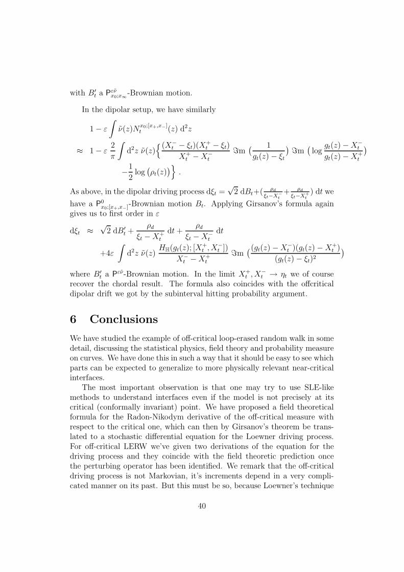
with B′t a P
ενx0;x∞
-Brownian motion.
In the dipolar setup, we have similarly
1 − ε
∫
ν(z)Nx0;[x+,x−]t (z) d2z
≈ 1 − ε2
π
∫
d2z ν(z){(X−
t − ξt)(X+t − ξt)
X+t −X−
t
ℑm( 1
gt(z) − ξt
)
ℑm(
loggt(z) −X−
t
gt(z) −X+t
)
−1
2log
(
ρt(z))
}
.
As above, in the dipolar driving process dξt =√
2 dBt+( ρd
ξt−X−t
+ ρd
ξt−X+t
) dt we
have a P0x0;[x+,x−]-Brownian motion Bt. Applying Girsanov’s formula again
gives us to first order in ε
dξt ≈√
2 dB′t +
ρd
ξt −X+t
dt+ρd
ξt −X−t
dt
+4ε
∫
d2z ν(z)HH(gt(z); [X
+t , X
−t ])
X−t −X+
t
ℑm((gt(z) −X−
t )(gt(z) −X+t )
(gt(z) − ξt)2
)
where B′t a P
εν-Brownian motion. In the limit X+t , X
−t → ηt we of course
recover the chordal result. The formula also coincides with the offcriticaldipolar drift we got by the subinterval hitting probability argument.
6 Conclusions
We have studied the example of off-critical loop-erased random walk in somedetail, discussing the statistical physics, field theory and probability measureon curves. We have done this in such a way that it should be easy to see whichparts can be expected to generalize to more physically relevant near-criticalinterfaces.
The most important observation is that one may try to use SLE-likemethods to understand interfaces even if the model is not precisely at itscritical (conformally invariant) point. We have proposed a field theoreticalformula for the Radon-Nikodym derivative of the off-critical measure withrespect to the critical one, which can then by Girsanov’s theorem be trans-lated to a stochastic differential equation for the Loewner driving process.For off-critical LERW we’ve given two derivations of the equation for thedriving process and they coincide with the field theoretic prediction oncethe perturbing operator has been identified. We remark that the off-criticaldriving process is not Markovian, it’s increments depend in a very compli-cated manner on its past. But this must be so, because Loewner’s technique
40

reduces the future of the curve to the original setup by conformal maps andthe off-critical model is not conformally invariant.
We hope that this example encourages studies of interfaces in other off-critical models, some maybe physically more relevant. Furthermore, evenafter the novel connections of LERW to field theory, there clearly remainsimportant questions to be understood before we have a fully satisfactory fieldtheory description of LERWs.
A Random walks as an example
The example of random walks in 1D can serve as a trivial illustration ofthe themes discussed in this article. Suppose we weight walks on Z startingfrom 0 by giving weight µeγ > 0 to each positive step and µe−γ > 0 toeach negative step. The weight of a walk of n steps ending at s is simplyµnesγ if −n ≤ s ≤ n and n − s is even, but 0 otherwise. The partitionfunction Z, obtained by summing over all paths, converges if and only ifw ≡ 2µ cosh γ < 1, and then Z = 1
1−w. We infer that the average length
of a path is µ∂ log Z∂µ
= w(1−w)2
which goes to +∞ as w approches 1−. Hencea critical theory is obtained for w = 1 i.e. when the weight of walks oflength n is 1 for each n and the model has a purely probabilistic randomwalk description. Hence the critical line is 2µ cosh γ = 1.
The quadratic fluctuation of the end point of the walk is(
λ ∂∂λ
)2logZ =
w−w2+v2
(1−w)2where v ≡ 2µ sinh γ. For fixed v 6= 0, this blows up like the average
length of the walk for w → 1−, but for v = 0 the divergence is milder. Hencethe point γ = 0, which is nothing but the simple symmetric random walk, isspecial among the critical points. At v = 0, the weight of a path of length nis simply (w/2)n and a continuum limits exist for which log(w/2) scales likethe square of the lattice spacing, leading in the continuum to weight pathsby the local time, as used at length in these notes in the 2D situation.
But for now, let us concentrate on the critical line. The weight of an nsteps path ending at Sn is eγSn(2 cosh γ)−n and the ratio of this weight tothat of the simple symmetric random walk is Qn = eγSn(cosh γ)−n which isreadily checked to be a martingale for the simple symmetric random walk.As in the continuum, this martingale can be used to change the measure to anew one under which the symmetric random walk is turned to an asymmetricone. We get this trivially in the discrete setting, but in more complicatedsituations, the flexibility offered by the continuum theory and Girsanov’stheorem is invaluable. So we turn to the continuum limit.
Introduce a lattice spacing a so that the macroscopic position after n steps
41

is aSn. If this has a continuum limit and the martingale Qn as well, one musttake γ ∼ ag and, in order for the second factor (cosh γ)−n to converge, onehas to set a2n = t and keep t fixed when taking the lattice spacing to 0,
defining aSn → Xt in the limit. Then Qn goes to Mt = egXt−g2t2 . If Xt is a
1D Brownian motion dXt = dBt, with quadratic variation (dBt)2 = dt, then
Mt is well known to be a martingale, well-defined for t <∞ finite, normalizedto M0 = 1 and such that M−1
t dMt = gdBt.With respect to the dressed expectation E[· · · ] = E[· · ·Mt], the process
Xt satisfies dXt = dBt + gdt with Bt a Brownian motion with respect toE[· · · ].
In particular, it is easy to check that E[XtMt] = gt. More generally,for any function F (Xt) we have d
dtE[F (Xt)] = E[A · F (Xt)] with dressed
stochastic evolution operator A · F (Xt) = gF ′(Xt) + 12F ′′(Xt). This indeed
corresponds to the stochastic equation dXt = dBt + gdt. This follows fromdirect computation using the Ito derivative M−1
t d(F (Xt)Mt) = (gF (Xt) +12F ′(Xt))dBt + (gF ′(Xt) + 1
2F ′′(Xt))dt.
This naıve example can also serve as a warning. It is well known thatthe percolation interface on a domain cut in the hexagonal lattice can beconstructed as an exploration process. If the beginning of the interface isconstructed, its last step separates two hexagons of different colors, and itsend touches a third hexagon. Either this third hexagon has already beencolored or one tosses a coin to decide the color, and then the path makesanother step along an edge separating two hexagons of different colors. Theinterface ends when it exits the domain. Hence one can encode each interfaceby a coin tossing game (of random duration). If the domain is the upper halfplane, the length of the game is always infinite, and there is a simple one toone correspondance between percolation interfaces and random walks (simplein principle, there is some subtlety hidden in the fact that sometimes one canmake one or several interface steps without the need to toss a coin, so thatthe number of steps of the interface is not simply related to the numberof coin tossings). Critical percolation corresponds to the simple symmetricrandom walk with w = 1, v = 0. As recalled in the main text, the scalingregion for critical percolation leads to a scaling v ∼ a3/4. On the other hand,the scaling region for the random walk is v ∼ a ≪ a3/4. This means that ifone uses a random walk with a (non critical) scaling limit, the correspondingpercolation interface is still critical, and symmetrically that if one looks ata percolation interface in the (non critical) scaling limit, the correspondingrandom walk is not described by the scaling region.
42

Aknowledgements: We wish to thank Vincent Beffara, Julien Dubedat,Greg Lawler, Stas Smirnov and Wendelin Werner for discussions at variousstages of this work.
Our work is supported by ANR-06-BLAN-0058-01 (D.B.), ANR-06-BLAN-0058-02 (M.B.) and ENRAGE European Network MRTN-CT-2004-5616 (M.B.and K.K.).
References
[1] Michel Bauer and Denis Bernard: 2D growth processes: SLE andLoewner chains. Phys. Rep., 432(3-4):115-222, 2006.
[2] Michel Bauer and Denis Bernard: Conformal field theories of stochasticLoewner evolutions. Comm. Math. Phys., 239(3):493–521, 2003.
[3] Michel Bauer and Denis Bernard: SLE, CFT and zig-zag probabili-ties. Proceedings of the conference ‘Conformal Invariance and RandomSpatial Processes’, Edinburgh, July 2003.
[4] M. Bauer, D. Bernard and J. Houdayer: Dipolar SLEs. J. Stat. Mech.0503:P001, 2005.
[5] M. Bauer, D. Bernard and T.G. Kennedy: in preparation.
[6] Michel Bauer, Denis Bernard, and Kalle Kytola: Multiple Schramm-Loewner evolutions and statistical mechanics martingales. J. Stat. Phys.,120(5-6):1125–1163, 2005.
[7] A.A. Belavin, A.M. Polyakov and A.B. Zamolodchikov: Infinite confor-mal symmetry in two-dimensional quantum field theory. Nucl. Phys. B241 (1984), 333–380.
[8] F. Camia, L. Fontes and C. Newman: The scaling limit geometry ofnear-critical 2d percolation. [arXiv:cond-mat/0510740].
[9] Sergio Caracciolo, Jesper Lykke Jacobsen, Hubert Saleur, Alan D. Sokaland Andrea Sportiello: Fermionic Field Theory for Trees and Forests.Phys. Rev. Lett. 93, 080601 (2004).
[10] John Cardy: Scaling and renormalization in statistical physics. Cam-bridge University Press, 1996.
43

[11] John Cardy: SLE for theoretical physicists. Ann. Physics 318 (1):81–118, 2005.
[12] W. Kager and B. Nienhuis: A guide to stochastic Lowner evolution andits applications J. Stat. Phys. 115 (5-6):1149–1229, 2004.
[13] Horst G. Kausch: Symplectic Fermions. Nucl. Phys. B 583 (2000) 513-541
[14] Tom G. Kennedy: The Length of an SLE – Monte Carlo Studies J.Stat. Phys., to appear. Preprint version: [arXiv:math/0612609v2]
[15] Kalle Kytola: On conformal field theory of SLE(kappa, rho). J. Stat.Phys., 123(6):1169–1181, 2006.
[16] Kalle Kytola: Virasoro Module Structure of Local Martingales of SLEVariants. Rev. Math. Phys., 19(5):455–509, 2007.
[17] Gregory F. Lawler: Conformally invariant processes in the plane. Math-ematical Surveys and Monographs 114. American Mathematical Society,Providence, RI, 2005.
[18] Gregory F. Lawler: Dimension and natural parametrization for SLEcurves. available on the author’s webpage.
[19] Gregory F. Lawler, Oded Schramm, and Wendelin Werner: Conformalinvariance of planar loop-erased random walks and uniform spanningtrees. Ann. Probab., 32(1B):939–995, 2004.
[20] Gregory Lawler, Oded Schramm, and Wendelin Werner: Conformalrestriction: the chordal case. J. Amer. Math. Soc., 16(4):917–955 (elec-tronic), 2003.
[21] Gregory F. Lawler and Scott Sheffield: Construction of the naturalparametrization for SLE curves. in preparation.
[22] Gregory F. Lawler and Wendelin Werner: The Brownian loop soup.Probab. Theory Related Fields 128:4 565–588 (2004).
[23] Satya Majumdar: Exact fractal dimension of the loop-erased self-avoiding walk in two dimensions. Phys. Rev. Lett. 68, 2329 - 2331 (1992).
[24] N. Makarov and S. Smirnov: Massive SLEs. in preparation.
[25] Pierre Nolin and Wendelin Werner: Asymmetry of near-critical perco-lation interfaces. preprint, [arXiv:0710.1470].
44

[26] Oded Schramm: Scaling limits of loop-erased random walks and uniformspanning trees. Israel J. Math., 118:221–288, 2000.
[27] O. Schramm and D. Wilson: SLE coordinate changes. NY J. Math. 11(2005), 659-669.
[28] S. Smirnov: Critical percolation in the plane: conformal invariance,Cardy’s formula, scaling limits. C. R. Acad. Sci. Paris 333(2001), 239-244.
[29] Wendelin Werner: Random planar curves and Schramm-Loewner evo-lutions. Lectures on probability theory and statistics. Lecture Notes inMath. 1840:107-195. Springer, Berlin.
[30] David B. Wilson: Generating random spanning trees more quickly thanthe cover time. Proceedings of the Twenty-eighth Annual ACM Sym-posium on the Theory of Computing (Philadelphia, PA, 1996), 296-303,ACM, New York, 1996.
[31] Dapeng Zhan: The Scaling Limits of Planar LERW in Finitely Con-nected Domains. Ann. Probab. (to appear)
45