leopard: lightweight edge-oriented partitioning …leopard: lightweight edge-oriented partitioning...
TRANSCRIPT

LEOPARD: Lightweight Edge-Oriented Partitioning andReplication for Dynamic Graphs
Jiewen HuangYale University
Daniel J. AbadiYale University
ABSTRACTThis paper introduces a dynamic graph partitioning algo-rithm, designed for large, constantly changing graphs. Wepropose a partitioning framework that adjusts on the fly asthe graph structure changes. We also introduce a replica-tion algorithm that is tightly integrated with the partition-ing algorithm, which further reduces the number of edgescut by the partitioning algorithm. Even though the pro-posed approach is handicapped by only taking into consider-ation local parts of the graph when reassigning vertices, ex-tensive evaluation shows that the proposed approach main-tains a quality partitioning over time, which is comparableat any point in time to performing a full partitioning fromscratch using a state-the-art static graph partitioning algo-rithm such as METIS. Furthermore, when vertex replicationis turned on, edge-cut can improve by an order of magnitude.
1. INTRODUCTIONIn recent years, large graphs are becoming increasingly
prevalent. Such graph datasets are too large to manage ona single machine. A typical approach for handling data atthis scale is to partition it across a cluster of commodity ma-chines and run parallel algorithms in a distributed setting.Indeed, many new distributed graph database systems areemerging, including Pregel [22], Neo4j, Trinity [34], Horton[30], Pegasus [15], GraphBase [14], and GraphLab [21].
In this paper, we introduce data partitioning and replica-tion algorithms for such distributed graph database systems.Our intention is not to create a new graph database system;rather our data partitioning and replication algorithms canbe integrated with existing scalable graph database systemsin order to improve the performance of the current imple-mentation of their parallel query execution engines.
The most common approach for partitioning a large graphover a shared-nothing cluster of machines is to apply a hashfunction to each vertex of the graph, and store the vertexalong with any edges emanating from that vertex on themachine assigned to that hash bucket. Unfortunately, hash
This work is licensed under the Creative Commons Attribution-NonCommercial-NoDerivatives 4.0 International License. To view a copyof this license, visit http://creativecommons.org/licenses/by-nc-nd/4.0/. Forany use beyond those covered by this license, obtain permission by [email protected] of the VLDB Endowment, Vol. 9, No. 7Copyright 2016 VLDB Endowment 2150-8097/16/03.
partitioning graph data in this fashion can lead to subopti-mal performance for graph algorithms whose access patternsinvolve traversing the graph along its edges. For example,when performing subgraph pattern matching, patterns arematched by successively traversing a graph along edges frompartially matched parts of the graph. If the graph is parti-tioned in a way that nodes close to each other in the graphare physically stored as close to each other as possible, thenetwork traffic of such graph algorithms can be significantlyreduced.
In general, there are two goals that are desirable from apartitioning algorithm for workloads with traversal-orientedaccess patterns. First, if two vertices are connected by anedge, it is desirable for those two vertices to be stored onthe same physical machine. If a partitioning algorithm as-signs those vertices to two different machines, that edge isreferred to as being “cut”. Second, the size of the subgraph(in terms of the number of vertices and edges) stored oneach partition should be approximately equal, so that graphalgorithms can be parallelized equally across the cluster formaximum performance. These two goals are often in con-flict. For example, it is easy to guarantee that no edge is evercut if the entire graph is stored on a single machine, How-ever, the partitioning would be extremely unbalanced, andgraph algorithms would not be able to leverage the parallelresources in the cluster. On the other hand, hash parti-tioning usually gets near perfect balance of assignment ofvertices and edges to nodes, but yields a high number of cutedges.
The dual goals of minimizing edge cut and maintainingbalanced partitions is usually formulated as the k-balancedpartitioning problem. k-partitioning has been studied exten-sively, and there exist many k-partitioning algorithms, bothin the theoretical space, and some which have practical im-plementations. However, almost all of these k-partitioningalgorithms run on static graphs — namely, the whole graphis known before the partitioning algorithm starts. The bestknown of these include METIS [17] and Chaco [12], whichgo through multiple levels of coarsening and refinement. Re-cent work includes lighter-weight algorithms that make sev-eral passes through the static graph and partition it withoutstoring the entire graph in memory [35, 37, 25].
While getting a good initial partitioning of a static graphis certainly important, many modern graphs are dynamic,with new vertices and edges being added at high rates, andin some cases vertices and edges may be removed. There-fore, a good initial partitioning may degrade over time. Itis inefficient to repeatedly run the static graph partitioning
540
algorithm to repartition the entire graph every time the par-titioning starts to degrade a little. Instead, it is preferableto incrementally maintain a quality graph partitioning, dy-namically adjusting as new vertices and edges are added tothe graph. For this reason, there has been several recentresearch efforts in dynamic graph partitioning [33, 32, 31,40, 39, 42].
Another important aspect of distributed systems is repli-cation for fault tolerance by replicating data across severalmachines/nodes so that if one node fails, the data can stillbe processed by replica nodes. In general, the level of faulttolerance is specified by a minimum number of copies. If theentire subgraph stored on a particular node is replicated toan equivalent replica node, then replication can be consid-ered completely independently from partitioning. However,more complicated replication schemes are possible where dif-ferent parts of the subgraph stored on a node are replicatedto different nodes depending on which nodes store subgraphs“closest” to that particular part of the subgraph. Replicat-ing data in this way can significantly improve the edge-cutgoals of partitioning, while maintaining the required faulttolerance guarantees.
One possible replication algorithm is to make replicas ofall non-local neighbors for every vertex in the graph [27, 13]so that all accesses for neighbors are local. Unfortunately,many graphs contain “high degree” vertices (vertices asso-ciated with many edges), which end up getting replicatedto most (if not all) nodes under such a replication algo-rithm. The effect is thus that some vertices get replicatedfar more than the minimum level required for fault toler-ance, while other “low degree” vertices do not get replicatedat all. A good replication algorithm needs to ensure a min-imal replication for each vertex, while judiciously using anyextra replication resources to replicate those vertices thatwill benefit the partitioning algorithm the most.
One problem with replication is keeping the replicas insync. For graphs where the vertices contain attributes thatare updated frequently, the update cost is multiplied by thenumber of replicas. Furthermore, many bulk-synchronousparallel (BSP) graph processing algorithms (such as well-known implementations of page rank, shortest paths, andbipartite matching [22]) work by updating ongoing calcula-tions at each vertex upon each iteration of the algorithm.Enforcing replication of these running calculations at eachiteration cancels out the edge-cut benefits of replication.
Previous approaches to dynamic graph partitioning weredesigned for graph applications where computations involvefrequent passing of data between vertices. Therefore, theydo not consider replication as a mechanism to reduce edge-cut, since the cost of keeping replicas in sync with each otherduring the computation is too high. In contrast, our workfocuses on workloads that include read-only graph computa-tions. While vertices and edges may be frequently added ordeleted from the graph, and they may even occasionally beupdated though explicit graph update operations, the pro-cessing operations over the graph fall into two categories —“read-only” and “non-read-only”. Replication has the po-tential to improve the locality of read-only operations with-out hindering the performance of non-read-only operationsthat involve writing temporary data that can be deleted atthe end of the computation (since the replicas can be ignoredin such a scenario). Perhaps the most common read-onlyoperation is sub-graph pattern matching and graph isomor-
phism — such operations are prevalent in SPARQL databasesystems where queries are expressed as a subgraph patternmatching operation over RDF data. However, read-only op-erations are also common for other types of graph systems.For example, triangle finding over social network data is animportant tool for analyzing the properties of the network.
The primary contribution of our work is therefore the in-troduction of the first (to the best of our knowledge) dy-namic graph partitioning algorithm that simultaneously in-corporates replication alongside dynamic partitioning. Wefirst propose a new, lightweight, on-the-fly graph partition-ing framework that incorporates new edges instantly, andmaintains a quality partitioning as the graph structure changesover time. Our approach borrows techniques and calcula-tions from single-pass streaming approaches to (non-dynamic)graph partitioning. We leverage the flexibility of the stream-ing model to develop a vertex replication policy that dra-matically improves the edge-cut characteristics of the par-titioning algorithm while simultaneously maintaining faulttolerance guarantees. Since the reduction in edge-cut that isderived from replication is only applicable for certain graphoperations, we also contribute a model that specifies the ef-fective edge-cut of a replicated graph given a specific classof graph algorithm.
We also run an extensive evaluation of Leopard — an im-plementation of our dynamic partitioning and replicationalgorithm — on eleven graph data sets from various do-mains: Web graphs and social graphs and synthetic graphs.We find that even without replication, our stream-based dy-namic partitioning approach produces an “edge-cut” similarto the edge-cut of the same graph if it had been repartitionedusing a state-of-the-art static partitioning algorithm at thatpoint in time. However, once replication is turned on, Leop-ard produces edge-cuts many factors smaller — in two casestransforming datasets with 80% edge-cut to 20% edge-cut.
2. BACKGROUND AND RELATED WORKEven without considering dynamic graphs, static graph
partitioning by itself is an NP-hard problem [11] — eventhe simplest two-way partitioning problem is NP-hard [10].There are several linear programming-based solutions thatobtain an O(log n) approximation for k-way partitioning[1, 8]. However, these approaches tend to be impracti-cal. Various practical algorithms have been proposed thatdo not provide any performance guarantees, but prove effi-cient in practice. For small graphs, algorithms such as KL[19] and FM [9] are widely used. For large graphs, thereare several multi-level schemes, such as METIS [17], Chaco[12] , PMRSB [3] and Scotch [26]. These schemes first gothrough several levels of coarsening to roughly cut the graphinto small pieces, then refine the partitioning with KL [19]and/or FM [9] and finally project the pieces back to the finergraphs. These algorithms can be parallelized for improvedperformance, such as in ParMetis [18] and Pt-Scotch [5]. Tohandle billion-node graphs, Wang et al. [41] design a multi-level label propagation method on top of Trinity [34]. Itfollows the framework of coarsening and refinement, but re-places maximal match with a label propagation [29] methodto reduce memory footprint.
Most of the research on partitioning of dynamic graphsfocus on repartitioning the graph after a batch of changesare made to an original partitioning that cause the originalpartitioning to deteriorate [33]. In general, two approaches
541

are used. The first approach is scratch-map partitioning,which simply performs a complete partitioning again usinga static partitioner [32]. The second (more commonly used)approach is diffusive partitioning. It consists of two steps:(1) a flow solution that decides how many vertices shouldbe transferred between partitions using linear programmingand (2) a multi-level diffusion scheme that decides whichvertices should be transferred [31, 40]. These repartition-ing schemes are heavyweight and tend to process a batchof changes instead of one change at a time. Furthermore,they tend to come from the high performance computingcommunity, and do not consider replication alongside parti-tioning. In contrast, in this paper we focus on light-weightdynamic partitioning schemes that continually update thepartitioning as new changes are streamed into the system,and tightly integrate replication with partitioning.
More recent works introduce light-weight partitioning al-gorithms for large-scale dynamic graphs. Vaquero et al. [39]propose a framework that makes use of a greedy algorithmto reassign a vertex to a partition with the most neighbors,but at the same time defers some vertex migration to ensureconvergence. Xu et al. [42] propose methods for partitioningbased on a historical log of active vertices in a graph pro-cessing system. Our work differs from theirs since we do notassume any kind of historical information of how the graphis processed. More importantly, the systems proposed byVaquero and Xu et al. are designed for BSP graph process-ing systems that continuously update vertices in the graphwith temporary data associated with running computations.Therefore, they do not consider replication as a mechanismfor improving edge-cut, due to the overhead of keeping repli-cas updated with this temporary data. In contrast, a centralcontribution of our work is the consideration of read-onlygraph algorithms (such as subgraph pattern matching oper-ations, triangle finding, and certain types of graph traversaloperations) for which replication of data has the potentialto reduce edge-cut and greatly improve the performance ofthese read-only operations. Thus the integration of parti-tioning and replication is the focus of our work, but not theother works cited above.
There have been several recent papers that show howtreating replication as a first class citizen in graph databasesystems can greatly improve performance. Pujol et al. [27]use replication to ensure that neighbors of a vertex are al-ways co-located in the same partition as the vertex. In otherwords, if a vertex’s neighbors are not originally placed in thesame partition as a vertex, they are replicated there. How-ever, such a strong guarantee comes with significant over-head — high degree vertices get replicated a large numberof times, and keeping the replicas consistent requires sig-nificant communication. Mondal and Deshpande fix thisproblem by defining a novel fairness requirement to guidereplication that ensures that a fraction of neighbors (but notnecessarily all neighbors) of a vertex be located in the samepartition [23]. Furthermore, they use a clustering scheme toamortize the costs of making replication decisions. However,the main focus of the Mondal and Deshpande paper is repli-cation, and their system is built on top of a hash partitioner.In contrast, our work focuses on reducing edge-cut througha combination of light-weight graph partitioning and repli-cation. Partitioning and replication are built together as asingle component in Leopard, and work in conjunction toincrease locality of query processing.
Duong et al. show that another important benefit of repli-cation is to alleviate load skew at query time [7]. Withoutreplication, the partitions that store “popular nodes” getoverwhelmed with requests for the values of those nodes.Replicating these popular nodes spreads out the resourcesavailable to serve these requests and reduces load skew. Sim-ilar to the work by Pujol et al. and Mondal and Deshpande,the replication scheme performed by Duong et al. also re-duces edge-cut by using the number of neighbors in a localpartition to guide the replication algorithm. The algorithmpresented by Duong et al. is for the complete partitioning ofa graph. This work does not discuss incremental repartition-ing as the graph structure changes over time (this is explictlyleft by Duong et al. for future work). In contrast, our fo-cus in this paper is on the dynamic repartitioning problem.The integration of replication considerations into dynamicrepartitioning algorithms is non-trivial, and has not beenaddressed by the above-cited related work.
Leopard’s light-weight dynamic graph partitioning algo-rithm builds on recent work on light-weight static partition-ers. These algorithms partition a graph while performing asingle pass through the data — for each vertex read fromthe input graph dataset, they immediately assign it to apartition without the knowledge of the vertices that will beread afterward. Because of the online nature of these algo-rithms, lightweight heuristics are often used to decide whereto assign vertices, including the linear deterministic greedy(LDG) approach [35] and FENNEL [37]. LDG uses mul-tiplicative weights to maintain a balanced partitioning andFENNEL leverages modularity maximization [4, 24] to de-ploy a greedy strategy for maintaining balanced partitions.Nishimura and Ugander [25] advanced this work by intro-ducing several-pass partitioning and stratified partitioning.Similarly, Ugander and Backstrom introduce an iterative al-gorithm where each iteration does a full pass through thedata-set and uses a linear, greedy, label propagation algo-rithm to simultaneously optimize for edge locality and parti-tion balance [38]. However, the single-pass algorithms, alongwith the Nishimura et. al. and Ugander et. al. algorithmsare designed to be run on demand, in order to occasionally(re)partition the entire graph as a whole. Furthermore, theydo not consider replication. In contrast, our focus in this pa-per is on continuously repartitioning a graph in a lightweightfashion as it is dynamically modified. Furthermore, we ex-plicity consider replication for fault tolerance as a tool forsimultaneously improving partitioning.
3. VERTEX REASSIGNMENTOne key observation that serves as the intuition behind
Leopard, is that the dynamic graph partitioning problemis similar to the one-pass partitioning problem [35, 37] de-scribed in Section 2. In many cases, what makes most dy-namic graphs dynamic are new vertices and edges that areadded. Therefore at any point in time, a dynamic graphcan be thought of as an intermediate state in the midst of aone-pass partitioning algorithm. Consequently, the heuris-tics that have been used for one-pass algorithms can be lever-aged by Leopard.
The intuition behind the one-pass streaming heuristics isthe following: to achieve a low cut ratio, a new vertex shouldbe assigned to the existing partition with most of its neigh-bors. However, at the same time, a large partition shouldbe penalized to prevent it from becoming too large.
542

The FENNEL scoring heuristic is presented in Equation1. Pi refers to the vertices in the ith partition. v refersto the vertex to be assigned and N(v) refers to the set ofneighbors of v. α and γ are parameters.
argmax1≤i≤k
{|N(v) ∩ Pi| − αγ
2(|Pi|)γ−1}, (Equation 1)
This heuristic takes a vertex v as the input, computes ascore for each partition, and places v in the partition withthe highest score. |N(v) ∩ Pi| is the number of neighbors ofv in the partition. As the number of neighbors in a partitionincreases, the score of the partition increases. To ensure abalanced partitioning, it contains a penalty function basedon the number of vertices, |Pi|, in the partition. As thenumber of vertices increases, the score decreases.
While one-pass partitioning algorithms are able to get agood initial partitioning at very low overhead, they fall shortin three areas that are important for replicated, dynamicpartitioning (1) a vertex is assigned only once and nevermoves, (2) they do not consider deletes, and (3) they donot consider replication. Therefore, we cannot use a simpleadaptation of the one-pass streaming algorithms.
We first discuss the introduction of selective reassignmentinto streaming algorithms in this section. We defer the de-scription of the full dynamic partitioning algorithm that in-cludes a tight integration with replication to Section 4.
Example 1 illustrates a motivation for reassignment.
Example 1. Suppose there are two partitions P1 and P2.For the sake of simplicity of this example, we assume that thetwo partitions are roughly balanced at all times, so we onlyfocus on the number of neighbors of a vertex to determinewhere it should be placed.
After loading and placing the first 100 edges into differentpartitions, vertex v has 3 neighbors in P1 and 2 neighborsin P2. Hence, P1 is the better partition for v. However,after loading and placing another 100 edges, vertex v nowhas 4 neighbors in P1 and 10 neighbors in P2. The betterpartition for v is now P2. Therefore, the optimal partitionfor a vertex changes over time as new edges are added (ordeleted) — even though most of these new edges are addedto a partition different than where v is located.
Leopard therefore continuously revisits vertices and edgesthat have been assigned by the one-pass partitioning algo-rithm, and reassigns them if appropriate. Theoretically, allvertices could be examined for reassignment every time anedge is added (or deleted). However, this is clearly imprac-tical. Instead Leopard uses a more strategic approach.
When an edge (v1, v2) is added or deleted, most verticesare minimally affected. Only those vertices in the graphnear the edge are likely to be influenced enough to poten-tially justify a move. If v1 and v2 are located on differentpartitions, they become good candidates for reassignmentbecause they now have one additional (or less) neighbor ona different partition. In particular, v1 should perhaps bemoved to v2’s partition, or vice versa. This may cause aripple effect among neighbors of a reassigned vertex — oncea vertex moves to a new machine, its neighbors may also bebetter off being moved to a new machine.
Therefore, when a new edge (v1, v2) is added, v1 and v2 arechosen as the initial candidates for examination of potentialreassignment. If either one of them are reassigned, then the
immediate neighbors of the moved vertex are added to thecandidate set. This candidate set thus contains the set ofvertices immediately impacted by the recent graph activity.A subset of the vertices in this candidate set are examinedfor potential reassignment. This examination process in-volves reapplying the score function (e.g., Equation 1) tothese candidates. The algorithm for choosing the particularsubset of candidates that will be re-scored and potentiallyreassigned is given in the following section.
3.1 Timing of Reassignment ExaminationAfter examination candidates are chosen, Leopard must
decide whether examination should be performed on thosecandidates. As described above, examining a vertex v forreassignment involves calculating a score (e.g., Equation 1)for the placement of v on every partition in the cluster. Thisscoring process includes a calculation based on the numberof neighbors of v in each partition, which requires informa-tion to be accessed regarding where v’s neighbors are lo-cated. If the vertex location lookup table is small enoughto be hosted on one machine, then the cost of the lookupis small. However, for massive graphs, the lookup table isspread across the cluster, and this cost can be significant(Leopard uses a distributed consistent hash table [16] thatmaps vertex identifiers to their respective partitions). Ingeneral, examination comes with a non-negligible cost, andshould not be performed when there is little probability ofthe examination resulting in reassignment.
As a vertex’s number of neighbors increases, the influenceof a new neighbor decreases. For example, in one experi-ment that we ran in Section 6, a vertex with 10 neighbors isreassigned to a new partition upon receiving an 11th neigh-bor 13% of the time, while a vertex with 40 neighbors isreassigned to a new partition upon receiving a 41st neigh-bor only 2.5% of the time. Therefore, it is less cost-efficientto pay the reassignment examination cost for a vertex witha large number of existing neighbors, since it is likely thatthis examination work will be wasted, and the vertex willremain in its current partition.
Leopard therefore occasionally avoids the reassignmentexamination computation of a candidate vertex v if v alreadyhas many neighbors in the graph. Nonetheless, Leopard en-sures that even vertices with a large number of neighborsget examined periodically. The pseudocode for the logic onwhen to skip examination is shown in Figure 1. Given a ver-tex v and a threshold t, the function skips the computationof the reassignment scores if the ratio of skipped computa-tion to the total neighbors of v is less than t. This has theeffect of making the probability of performing reassignmentexamination after adding a new neighbor to v proportionalto (1− t)/(t)(v.neighbors).
Upon breaking up this formula into its two components,it can be seen that there are two factors that determinewhether an examination should be performed: 1/(v.neighbors)and (1− t)/t. This means that as the number of neighborsincreases, the probability of examination for reassignmentgoes down. At the same time, as t approaches 0, examina-tion will always occur, while as t approaches 1, examinationwill never occur.
There is clearly a tradeoff involved in setting t. A larger tskips more examinations and reduces the partitioning qual-ity, but improves the speed of the algorithm. Section 6 re-visits this tradeoff experimentally (see Figures 10 and 11).
543

Function ToExamineOrNot(v, threshold)
if an edge is added then
v.neighbors++
else if an edge is deleted then
v.neighbors−−end if
if (v.skippedComp + 1) ÷ v.neighbors ≥ threshold then
compute the reassignment scores for v
v.skippedComp = 0
else
v.skippedComp++
end if
Figure 1: Algorithm for deciding when to examine a vertexfor reassignment.
4. LEOPARD PARTITIONINGWe now present the complete Leopard partitioning algo-
rithm that tightly integrates replication with dynamic par-titioning.
Replication serves two purposes in Leopard: providingfault tolerance and improving access locality. Fault toler-ance is achieved by replicating vertices to different machines.By having n copies of each vertex, every vertex is still acces-sible even if the system loses n − 1 machines. Some graphdatabase systems are built on top of distributed file systemssuch as HDFS that provide their own replication mecha-nisms for fault tolerance. Such mechanisms are redundantwith Leopard’s replication and should be avoided if possiblewhen used in conjunction with Leopard (for example, HDFShas a configuration parameter that removes replication).
Better access locality improves performance. Even if anedge (v1, v2) is cut (meaning that v1 and v2 are in separatepartitions, which usually results in them being stored onseparate machines), if a copy of v2 is stored on v1’s partition(or vice versa), computation involving v1 and v2 may stillproceed locally without waiting for network communication.
Most systems treat replication for access locality and faulttolerance separately [7, 13, 27]. For example, a partitionerwill create an initial partitioning, and certain important ver-tices are selectively replicated to multiple partitions in or-der to reduce the edge-cut. Afterwards, entire partitions (orshards of partitions) are replicated to other machines forfault tolerance. This has the effect of “double-replicating”these important vertices. This may not be the most efficientuse of resources. A better edge-cut may have been achiev-able had additional important vertices been replicated dur-ing the first phase instead of double-replicating the originalset of important vertices. Leopard thus takes the approachof simultaneously considering access locality and fault tol-erance in order to avoid this waste of resources. It is im-portant to note, however, that recovery from failures aremore complicated when multiple shards or partitions needto be accessed in order to recover the data on the failedmachine. Although novel in the graph database space, thisapproach of trading off recovery complexity for improved re-source utilization has been performed before in the contextof column-store database systems. Different combinationsof columns (in potentially different sort orders) are storedon different machines, while ensuring that at least k copiesof each column are located across the cluster [36].
The primary downside to replication is the cost of keep-ing replicas in sync with each other. If an update to the
data stored inside a vertex must be performed, this updatemust be propagated to all replicas, and this must happenatomically if replicas are not allowed to not temporarily di-verge for a particular application. In this paper, we classifyupdates into two categories: permanent updates to funda-mental attributes of vertices or edges in a graph (e.g. chang-ing the name of a user in a social network), and temporaryupdates to vertices or edges that occur over the course ofa graph computation. In this section, we assume that theformer type of updates happen far less frequently than readsof these vertices or the addition or removal of vertices andedges. However, several solutions have been proposed in theresearch community for how to handle replication when thisassumption does not hold [6, 28]. We make no assumptionsabout the latter type of updates (temporary updates) anddiscuss them in more detail below.
4.1 Replication, Access Locality and CutAn access from a vertex v to a neighbor u is local if v and
u are placed on the same machine. Otherwise it is remote.When vertices are not replicated, this is directly related towhether edge (v, u) is cut, and edge cut ratio can be used topredict access locality. However, the definition of cut ratiois more complicated when considering vertex replication.
Figure 2 illustrates this complexity for a sample graphcontaining vertices in triangle. In the case without replica-tion (a), all three edges are cut. In the case with replication(b), A,B and C are replicated to partitions 3, 1 and 2, re-spectively. It could be argued that the edge (A,B) is nolonger cut, since partition 1 now contains a copy of both Aand B. By the same logic, the edge (A,C) would no longerbe cut since partition 3 now contains both vertices. How-ever, if a query wanted to access A, B, and C, this querycannot be performed locally. In other words, even thoughthe edge (A,B) is not cut, and the edge (A,C) is not cut,we cannot transitively deduce that A, B, and C are in thesame partition. In contrast, in a system without replication,such a transitive property would hold.
A B
C
Partition 1 Partition 2
Partition 3
(a) Partitioning without replication
Partition 3
Partition 2Partition 1
A B
C
B’ C’
A’
(b) Partitioning with replication
Figure 2: Partitions without and with replication. A′, B′
and C′ are replicas.
The fundamental problem is that replication adds a direc-tion to an edge. When B is replicated to A’s partition, itallows B to be accessed from the partition with the mastercopy of A. However, it does not allow A to be accessed fromthe partition with the master copy of B. Therefore half ofall co-accesses of A and B will be non-local (those that ini-tiate from B’s master copy) and half are local (those thatinitiate from A’s master copy). In other words, vertex repli-cation repairs the “cut” edges between the replicated vertexand all vertices on the partition onto which it is replicated,but these edges are only “half”-repaired — only half of allaccesses to that edge will be local in practice.
544
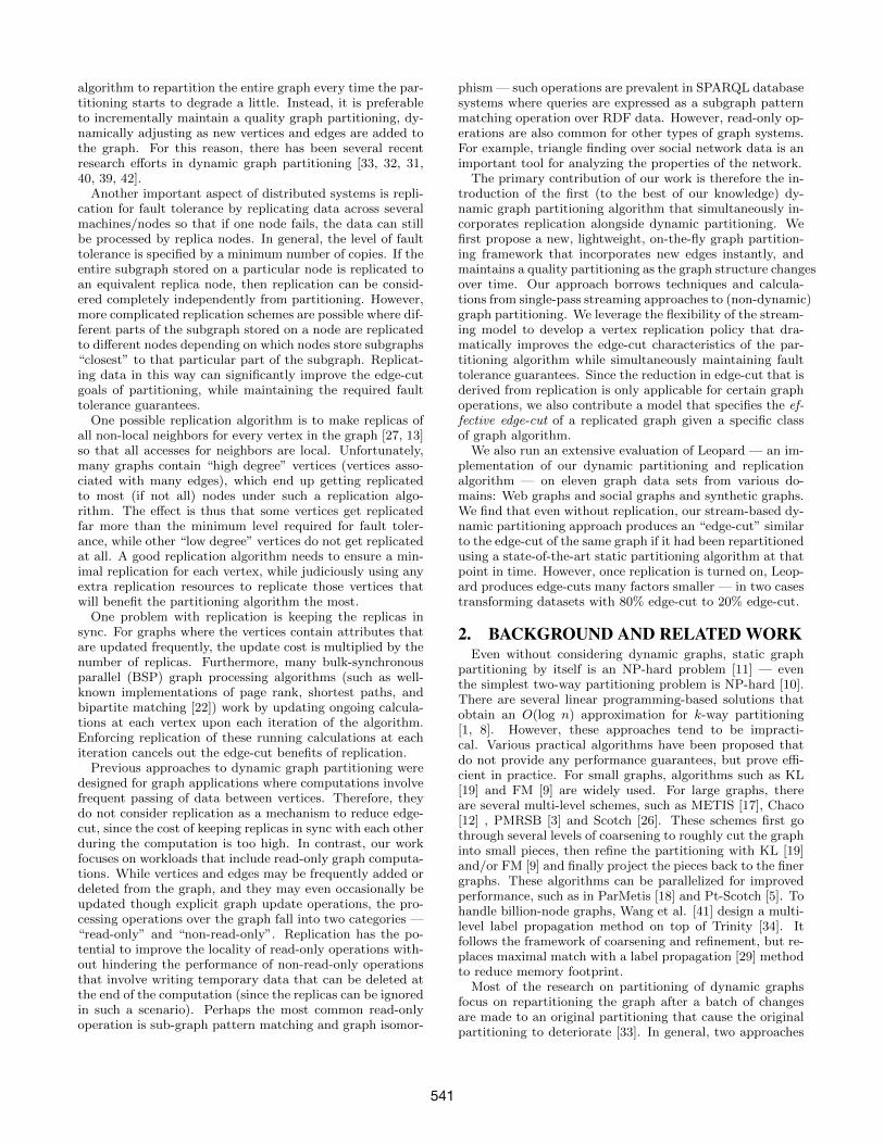
Furthermore, in some cases Leopard chooses to let thereplicas diverge. In particular, temporary data that is as-sociated with every vertex during an iterative graph com-putation (that is updated with each iteration of the com-putation) are not propagated to replicas. The reason forthis is that it only “pays off” to spend the cost of send-ing data over the network to keep replicas in sync if eachreplica will be accessed multiple times before the next up-date. For iterative graph computation where updates occurin every iteration, this multi-access requirement is not met.Therefore, Leopard does not propagate this temporary datato replicas during the computation, and thus replica nodescannot be used during the computation (since they containstale values). In such a scenario, the effective edge cut withreplication is identical to the edge cut without replication.
In order to accurately compare the query access locality ofan algorithm over a replicated, partitioned graph against thelocality of the same algorithm over an unreplicated graph,we focus on effective edge cut, which prevents an overstate-ment of the benefit of replication on edge-cut. In order toprecisely define effective edge cut, we classify all graph op-erations as either “read-only” and “non-read-only”. Read-only operations do not write data to vertices or edges of thegraph during the operation. For example, sub-graph pat-tern matching, triangle finding, and certain types of graphtraversal operations are typically read-only. In contrast,non-read-only operations, such as the iterative BSP algo-rithms discussed above, potentially write data to the graph.The effective edge cut is defined relative to the classifica-tion of a particular operation being performed on a graph.Given an operation, O, and an edge (u, v), Figure 3 pro-vides a value for the effective cut for that edge. When cal-culating the edge-cut for the entire graph, edges for whichDefineEffectiveCut returns “HALF CUT” have only halfof the impact relative to fully cut edges on the final edge-cut value. This accounts for the uni-directional benefit ofreplicating a vertex to a new partition.
Figure 4 shows examples corresponding to the four casespresented in the edge cut definition for read-only operations.
4.2 Minimum-Average ReplicationLeopard uses a replication scheme called MAR, an acronym
of Minimum-Average Replication. As the name suggests,the scheme takes two parameters: the minimum and averagenumber of copies of vertices. The minimum number of copiesensures fault tolerance and any additional copies beyond theminimum provides additional access locality. In general, theaverage number of copies specified by the second parametermust be larger than or equal to the first parameter. Figure5 shows an example graph with MAR.
Given a vertex, the MAR algorithm decides how manycopies of it should be created and in which partitions theyshould be placed. Leopard uses a two step approach. First, amodified version of the vertex assignment scoring algorithmis run. Second, the scores generated from the first step areranked along with recent scores from other vertices. Verticeswith a high rank relative to recent scores get replicated at ahigher rate than vertices with relatively low scores.
4.2.1 Vertex assignment scoring with replicationBecause of replication, the assignment score functions need
to be modified to accommodate the presence of secondarycopies of vertices and to remain consistent with the new edge
Function DefineEffectiveCut(v, u, O)
// p(v) and s(v) denote the primary copy
// and a secondary copy of v, respectively.
// O is the operation being performed on the graph.
if p(v) and p(u) are on the same partition then
return NOT CUT
else if p(v) and s(u) are on the same partition &
p(u) and s(v) are on the same partition then
if O is read-only
return NOT CUT
else
return CUT
else if p(v) and s(u) are on the same partition |p(u) and s(v) are on the same partition then
if O is read-only
return HALF CUT
else
return CUT
else
return CUT
end if
Figure 3: A definition of effective edge cut in the presenceof vertex replication.
v uEdge (v, u)
primary second. primary second.1 2,3 1 4,5 NO CUT1 2,3 2 1,3 NO CUT1 2,3 2 3,4 HALF CUT1 3,4 2 3,4 CUT
Figure 4: Examples of location of primary and secondarycopies and the corresponding cut for a read-only operation.A value of 2,3 in the secondaries column means that thesecondary copies are placed on partitions 2 and 3.
cut definition given in Section 4.1. In particular the scorefunction (see e.g., Equation 1) requires the list of all neigh-bors of the vertex being scored on each partition. Given avertex v that is currently being scored, we make the defini-tion of whether a vertex u is a neighbor of v in partition Pdependant on whether we are currently scoring the primaryor secondary copy of v:
Definition 1. Consider a graph G = (V,E). p(v) ands(v) denote the primary copy and a secondary copy of v,respectively. u is a neighbor of v on partition P if (v,u) ∈ Eand also one the following holds:(1) v is a primary copy and p(u) ∈ P(2) v is a primary copy and s(u) ∈ P(3) v is a secondary copy and p(u) ∈ P
Given that this definition is dependent on whether theprimary or secondary copy of v is being scored, Leopardcomputes two scores for each partition, P : one for the pri-mary copy of v and one for secondary copies. The primarycopy will be placed in the partition with the highest pri-mary copy score, and secondary copies are placed accordingto their scores using the algorithm presented in Section 4.2.2.
4.2.2 Ranking scores for secondary copiesAfter computing the score for a secondary copy of vertex
v for each candidate partition, these scores are sorted fromhighest to lowest. Since there is a minimum requirement of
545

K
BF
G
L
H
J
E
D
C
A
I
Input Graph
K
A
C
B’
G’
D’ I’
(a) Partition 1
B F L
K’
G’
A’
J’
(b) Partition 2
G
D I
C’
B’
E’
F’
H’
(c) Partition 3
H
J
E
F’
G’
I’
B’ L’
(d) Partition 4
Figure 5: Example of Minimum-Average Replication of an input graph, where the minimum = 2 and average = 2.5. Theprimary copy of each vertex is shown in light blue and their secondary copies are highlighted in a darker blue. 8 vertices have2 copies, 2 have 3 copies, and 2 (the best-connected vertices) have 4 copies. The copy of J in partition 2 does not improveaccess locality, but is required for fault tolerance.
Function ChoosePartitions(v, min, average)
choose a partition for the primary copy of v:
run the scoring algorithm for primary copy location
Pprimary = the partition with the highest score
Place primary copy of v on Pprimary
choose partitions for the secondary copies of v:
run the scoring algorithm for secondary location (
excluding Pprimary) and get a set of scores A
sort A from high to low
Pmin = (min− 1) partitions with the highest scores
B = all recently computed secondary copy scores
C = B⋃
A
sort C from high to low
/* k (see below) is the number of partitions */
Paverage = partitions whose score appear in the
top average−1k−1
of all scores
Psecondary = Pmin⋃
PaveragePlace secondary copies of v on partitions in Psecondary
Figure 6: An algorithm to choose partitions for the primaryand secondary copies for a vertex.
copies, M , necessary for fault tolerance, secondary copiesare immediately placed in the partitions corresponding tothe top (M − 1) scores. However, the MAR parameter cor-responding to the average number of copies, A, is usuallyhigher than M , so additional copies may be created. To de-cide how many copies to make, Leopard compares the scoresfor v with the s most recent scores for other vertices. Com-mensurate with the extent that the scores for v are higher orlower than the average scores for the s most recent vertices,Leopard makes the number of copies of v higher or lowerthan A. The specific details of how many copies are createdare presented in the algorithm in Figure 6.
There are two reasons why the comparison of v’s scoresare only made with the most recently computed scores ofs vertices, instead of all scores. First, for a big graph, thenumber of all computed scores is large. It is space consumingto store them and time consuming to rank them. Second, asthe graph grows larger, the scores tend to rise. Therefore,the scores computed at the initial stages are not comparableto the scores computed at later stages. The parameter s,representing the sliding window of score comparisons, is acustomizable parameter. In practice, s can be small (on theorder of 100 scores), as the function of this window is only toget a statistical sample of recent scores. Thus, this window
of scores takes negligible space and easily fits in memory.The following example illustrates how MAR works.
Example 2. Assume parameters of M (minimum) = 2and A (average) = 3 for MAR and the number of partitionsis 5. Also assume the sliding window s has a size of 24.
When running the vertex assignment scoring algorithm forthe primary copy of a vertex v, partitions 1 through 5 getscores of 0.15, 0.25, 0.35, 0.45 and 0.55, respectively. Sincepartition 5 has the highest score, it is chosen as the partitionfor the primary copy of v.
After running the vertex assignment scoring algorithm forthe secondary copies of v, partitions 1 through 4 get scoresof 0.1, 0.2, 0.3 and 0.4, respectively (partition 5 is excludedbecause it already has the primary copy). Since M is 2 andpartition 4 has the highest score, it is immediately chosenas the location for a secondary copy (to meet the minimumcopy requirement). Including partition 5, there are now twopartitions with copies of v.
The four scores for the secondary copies (i.e., 0.1, 0.2, 0.3and 0.4) are then combined with the 24 recent scores in thesliding window s and all 28 scores are then sorted. If anyof v’s three other secondary scores are in the top average−1
k−1
= 3−15−1
= 50% of all scores, then additional copies of v aremade for those partitions.
5. ADDING AND REMOVING PARTITIONSIn some circumstances, the number of partitions across
which the graph data is partitioned must change on the fly.In these cases, Leopard needs to either spread out data toinclude new partitions or concentrate the data to fewer par-titions. Decreasing the number of partitions is relativelystraightforward in Leopard. For every vertex placed on thepartitions to be removed, we run the vertex reassignmentscoring algorithm and assign it to the best partition accord-ingly. We will therefore now focus on adding new partitions.
A simple approach to adding a new partition would beto either use a static partitioner to repartition the entiregraph over the increased number of partitions, or to reloadthe entire graph in Leopard with a larger value for P (thenumber of partitions). Unfortunately, performing a scanthrough the entire graph to repartition the data is expensive,and is particularly poor timing if the reason why partitionsare being added is because machines are being added toaccommodate a currently heavy workload.
546
Graph |V| |E| Density Clustering Coef. Diameter [20] TypeWiki-Vote (WV) 7,115 100,762 3.9 ∗ 10−3 0.1409 3.8 Social
Astroph 18,771 198,050 1.1 ∗ 10−3 0.6306 5.0 CitationEnron 36,692 183,831 2.7 ∗ 10−4 0.4970 4.8 Email
Slashdot (SD) 77,360 469,180 1.6 ∗ 10−4 0.0555 4.7 SocialNotreDame (ND) 325,729 1,090,108 2.1 ∗ 10−5 0.2346 9.4 Web
Stanford 281,903 1,992,636 5.0 ∗ 10−5 0.5976 9.7 WebBerkStan (BS) 685,230 6,649,470 2.8 ∗ 10−5 0.5967 9.9 Web
Google 875,713 4,322,051 1.1 ∗ 10−5 0.5143 8.1 WebLiveJournal (LJ) 4,846,609 42,851,237 3.7 ∗ 10−6 0.2742 6.5 Social
Orkut 3,072,441 117,185,083 2.5 ∗ 10−5 0.1666 4.8 SocialBaraBasi-Albert graph (BA) 15,000,000 1,800,000,000 1.6 ∗ 10−5 0.2195 4.6 Synthetic
Twitter 41,652,230 1,468,365,182 1.7 ∗ 10−6 0.1734 4.8 SocialFriendster (FS) 65,608,366 1,806,067,135 8.4 ∗ 10−7 0.1623 5.8 Social
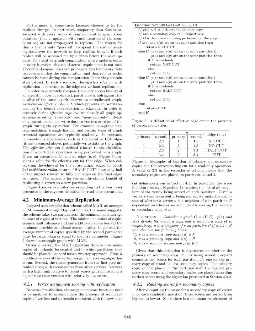
Figure 7: Statistics of the graphs used in the experiments. Diameter is reported at 90th-percentile to eliminate outliers.
Instead, Leopard first selects a group of vertices as seedsfor a new partition, and then runs the vertex reassignmentscoring algorithm on their neighbors, the neighbors of theirneighbors, the neighbors of the neighbors of their neighbors,and so on until all partitions are roughly balanced. Leop-ard proceeds in this order since the neighbors of the seedvertices that were moved to the new partition are the mostlikely to be impacted by the change and potentially alsomove to the new partition. This results in a requirement tocompute the reassignment scores for only a small, local partof the graph, thereby keeping the overhead of adding a newpartition small.
There are several options for the initial seeds for the newpartitions.• Randomly selected vertices from all partitions.• High-degree vertices from all partitions.• Randomly selected vertices from the largest partitions
(to the extent that there is not a perfect balance ofpartition size).
We experimentally evaluate these approaches in Section 6.4.
6. EVALUATION
6.1 Experimental SetupOur experiments were conducted on 4th Generation Intel
Core i5 and 16GB memory with Ubuntu 14.04.1 LTS.
6.1.1 Graph datasetsWe experiment with several real-world graphs whose sizes
are listed in Figure 7. They are collected from differentdomains, including social graphs, collaboration graphs, Webgraphs and email graphs. The largest graph is the Friendstersocial graph with 66 million vertices and 1.8 billion edges.
We also experiment with a synthetic graph model, thewell-known BaraBasi-Albert (BA) model [2]. It is an algo-rithm for generating random power-law graphs with pref-erential attachment. For the parameters to this model, weused n = 15,000,000, m = 12 and k = 15.
We transform all of these graphs into dynamic graphs bygenerating a random order of all edges, and streaming edgeinsertion requests in this order. Although this method forgenerating dynamic graphs does not result in deletions inthe dynamic workload, we have also run experiments thatinclude deletions in the workload, and observed identical re-sults due to the parallel way that Leopard handles additionsand deletions of edges.
6.1.2 Comparison PointsWe consider the following five partitioning approaches as
comparison points.
1. Leopard. Although Leopard supports any vertex as-signment scoring function, for these experiments we usethe same scoring function used by Tsourakakis et al.(FENNEL) [37]. As suggested by Tsourakakis et al., theFENNEL parameters we use throughout the evaluation
is γ = 1.5 and α =√k |E||V |1.5 . The sliding window we
use for the score ranking mechanism described in Section4.2.2 contains up to 30 recent vertices.
2. One-pass FENNEL partitioning. This comparisonpoint is a traditional one-pass streaming algorithm withthe FENNEL scoring function (with the same parametersas above). Like all traditional streaming algorithms, aftera vertex has been placed in a partition, it never moves.This comparison point is used to evaluate the benefit ofvertex reassignment in Leopard.
3. METIS [17]. METIS is a state-of-the-art, widely-usedstatic graph partitioning algorithm. It does not handledynamic graphs, so we do not stream update requests toMETIS the same way we stream them to Leopard andFENNEL. Instead, we give METIS the final graph, af-ter all update requests have been made, and perform astatic partitioning of this final graph. Obviously, having aglobal view of the final graph at the time of partitioning isa big advantage. Therefore, METIS is used as an approx-imate upper bound for partitioning quality. The goal forLeopard is to get a similar final partitioning as METIS,despite not having a global view of the final graph whilepartitioning is taking place.
4. ParMETIS [31]. ParMETIS is a state-of-the-art par-allel graph partitioning algorithm. It is designed for adifferent type of dynamic graph partitioning than Leop-ard. In particular, ParMETIS is designed for bulk repar-titioning operations after many vertices and edges havebeen added to the graph. This makes comparison toLeopard non-trivial. Leopard continuously maintains agood partitioning of a graph, while ParMETIS allows apartitioning to deteriorate and then occasionally fixes itwith its batch repartitioner. We thus report two sepa-rate sets of ParMETIS results — shortly before and afterthe batch repartitioner has been run. At any point in
547

0 %
10 %
20 %
30 %
40 %
50 %
60 %
70 %
80 %
90 %
100 %
WV Astroph Enron SD LJ Orkut Twitter FS BA BS Stanford ND Google
edge
cut
rati
o (
λ)
input graphs
One-pass FENNELLeopard
METISParMETIS (post-rp)ParMETIS (pre-rp)
Hash
Figure 8: Edge cut experiment. Cut ratio for hash parti-tioning is independent of the data set, and so it is displayedjust once on the left-hand side.
time, ParMETIS will have a partitioning quality in be-tween these two points. In order to present ParMETIS ina good light, we use FENNEL to maintain a reasonablequality partitioning in between repartitioning operationsas new vertices and edges are added to the graph (in-stead of randomly assigning new vertices and edges topartitions until the next iteration of the repartitioner).
5. Hash Partitioning. Most modern scalable graph databasesystems still use a hash function to determine vertex loca-tion. Therefore, we compare against a hash partitioner,even though it is known to produce many cut edges.
6.1.3 MetricsWe evaluate the partitioning approaches using two met-
rics: the edge cut ratio λ and load imbalance ρ, which aredefined as
λ =the number of edges cut
the total number of edges(For replicated data, a cut edge is defined as in Figure 3)
ρ =the maximum number of vertices in a partition
the average number of vertices in a partition.
6.2 Dynamic Partitioning
6.2.1 Comparison of SystemsIn this section, we evaluate partitioning quality in the
absence of replication. We partition the eleven real-worldgraphs into forty partitions using the five partitioning ap-proaches described above and report the results in Figure 8.The figure only presents the edge-cut ratio, since ρ (balance)is approximately the same for all approaches (it has a valueof 1.00 for hash partitioning and varies between 1.02 to 1.03for the other partitioners).
As expected, hash partitioning performs very poorly, sincethe hash partitioner makes no attempt to place neighboringvertices on the same machine. 39/40 (which is 97.5%) ofedges are cut, since with 40 partitions, there is a 1 in 40probability that a vertex happens to end up on the samepartition as its neighbor.
The “One-pass FENNEL” partitioner also performs poorly,since the structure of the graph changes as new edges areadded, yet the algorithm is unable to adjust accordingly.
When comparing this partitioner to Leopard, the impor-tance of dynamic reassignment of graph data becomes clear.On the other hand, Figure 8 does not present the compu-tational costs of partitioning. We found that the FENNELpartitioner completes a factor of 44.6 times faster than Leop-ard. So while Leopard’s partitioning is much better, it comesat significant computational cost. However, this experimentdid not use the skipping optimization described in Section3.1. In further experiments described below, we will findthat this factor of 44.6 computational difference can be re-duced to a factor of 2 with only small changes in cut ratio.
ParMETIS either performs poorly or well depending onhow recently the batch repartitioner has been run. For thisexperiment, the batch repartitioner ran after loading onefourth, one half, and three fourths of the vertices and edgesof the graph, and a fourth time at the end, after the entiregraph dataset had been loaded. We present two results forParMETIS - shortly before this final batch repartitioningis performed (labeled ParMETIS-pre-rp), and directly afterthe final repartitioning is performed (labeled ParMETIS-post-rp). ParMETIS-pre-rp is the worst case scenario forParMETIS — it has been the longest possible time sincethe last repartitioning. In this period of time, vertices andedges were added to the graph according to the FENNELheuristic. ParMETIS-post-rp is the best case scenario forParMETIS — it has just done a global repartitioning ofthe graph. Although ParMETIS’ repartitioning algorithmis lighter-weight than METIS’ “from-scratch” partitioningalgorithm, its edge-cut after this repartitioning operation isclose to METIS.
Surprisingly, Leopard is able to achieve a partitioning veryclose to METIS and ParMETIS’ best case scenario (post-rp),despite their advantage of having a global view of the finalgraph when running their partitioning algorithms. Since weuse METIS as approximate upper bounds on partitioningquality, it is clear that Leopard is able to maintain a highquality partitioning as edges are added over time.
Although Leopard achieves a good partitioning for all thegraphs, the quality of its partitioning relative to METIS ispoorest for the Web graphs. An analysis of the statistics ofthe graphs from Figure 7 shows that the Web graphs havelarge diameters. Graphs with large diameters tend to beeasier to partition. Indeed, a static partitioner with globalknowledge is able to cut less than 1 in 10 edges in the Webgraphs we used in our experiments. However, without thisglobal knowledge, Leopard enters into local optima whichresults in more edges being cut.
These local optima are caused by the balance heuristics ofthe streaming algorithm. Leopard’s scoring formula is de-signed to keep the size of each partition approximately thesame (as reported above, Leopard achieves a ρ-balance ofbetween 1.02 to 1.03). For graphs that are hard to par-tition, such as the power law graph we generated usingthe BaraBasi-Albert model, there are many vertices that nomatter where they are placed, they will result in many edgesbeing cut. Since the exact placement of these “problematic”vertices will not have a large effect on the resulting qualityof the partitioning, they can be placed in the partition thatwill most help to keep ρ low. In contrast, for partitionablegraphs, there are fewer of such “ρ-fixing” vertices, and occa-sionally vertices are placed on a partition with much fewerneighbors in order to avoid imbalance. This results in othervertices from the same partition to follow the original vertex
548

20 %
40 %
60 %
80 %
100 %
0 0.1 0.2 0.3 0.4 0.5 0.6 0.7 0.8 0.9
edge
cut
rati
o (
λ)
skipping threshold
OrkutGoogle
SlashdotEnron
Figure 9: Effects of skipping examination on edge cut ratio.
to the different partition. The end result is that sets of ver-tices that should clearly be part of one partition occasionallyend up on two or three different partitions.
This implies that Leopard should keep track of the neigh-bor locality and balance components of Equation 1 sep-arately. When there is frequent disparity between thesecomponents, Leopard should occasionally run a static parti-tioner as a background process, to readjust the partitioningwith a global view, in order to escape these local optima.
Although this experiment involves only adding new edges,we also ran an experiment where edges are both dynamicallyadded and deleted. We found that the inclusion of edge dele-tions in the experiment did not make a significant differencerelative to the workload with only addition of edges, sinceboth addition and removal of edges are treated as “relevant”events that cause reassignment to be considered. We do notpresent the results in more detail here due to lack of space.
6.2.2 SkippingIn Section 3.1 we described a shortcut technique, where
certain vertices with many existing neighbors (and are there-fore unlikely to be reassigned) are not examined for reassign-ment, even if a new edge adjacent to that vertex is added.In our previous experiment, this shortcut was not used. Wenow turn it on, and look more closely at how skipping ex-amination of vertices affects the edge cut ratio.
The results are shown in Figure 9. As expected, as the theskipping threshold increases (i.e., reassignment examinationis skipped more often), the quality of the cut suffers. Thelower the original cut ratio, the more damage skipping ver-tex examination can have on cut ratio. The Slashdot graphhas close to a 80% ratio without skipping and the 0.9 skip-ping threshold only increases the cut ratio to slightly above80%. On the other hand, Google Web graph’s cut ratio dra-matically jumps from 20% to 60%. However, for all graphs,skipping thresholds below 0.2 have a much smaller effect oncut ratio than higher thresholds.
Despite deteriorating the edge cut ratio, skipping vertexexamination can save resources by only forcing the systemto spend time examining vertices for reassignment if theyare likely to actually be reassigned as a result of the exam-ination. We define the savings as a fraction of the originalnumber of examined vertices, γ, as:
γ =number of vertices skipped for examination
number of vertices examined at threshold 0.
20 %
40 %
60 %
80 %
100 %
0 0.1 0.2 0.3 0.4 0.5 0.6 0.7 0.8 0.9
savin
g r
atio
(γ)
skipping threshold
TwitterOrkut
SlashdotEnron
Figure 10: Computation savings vs. skipping threshold.
0
0.1
0.2
0.3
0.4
0.5
0.6
0.7
0.8
0.9
1
0 0.1 0.2 0.3 0.4 0.5 0.6 0.7 0.8 0.9 1
run t
ime
rati
o t
o t
hat
w/o
skip
pin
g
skipping threshold
TwitterOrkut
SlashdotEnron
Figure 11: Run time improvement vs. skipping threshold.
A higher (lower) γ indicates higher (lower) savings of com-putation resources related to reassignment examination.
Figure 10 shows how changing the skipping threshold leadsto reassignment examination savings. For dense graphs suchas Orkut and Twitter (which have over 70 edges per vertex),a skipping threshold as low as 0.1 can result in an order ofmagnitude reduction in the reassignment examination workthat must be performed. For sparser graphs, the benefits ofskipping vertex examination are less significant.
Figure 11 shows how this reassignment examination sav-ings translates to actual performance savings. The figureshows the end-to-end run-time as a ratio to that withoutskipping of the partitioning algorithm for the same experi-ment that was performed in Section 6.2.1. When comparingthe extreme left- and right-hand sides of the graph, the costof too much vertex reassignment is evident. The extremeright-hand side of the graph (where the skipping ratio is 1),results in there never being any reassignment ever. Leop-ard simply loads the vertices and edges one by one, andnever moves a vertex from its initial placement. The ex-treme left-hand side of the graph corresponds to the fullreassignment examination policy without any skipping. Itis consistent with Figure 10 that skipping is more benefi-cial for denser graphs. We will use Orkut as an exampleto illustrate the benefit of skipping. The total time to passthrough the Orkut graph without any reassignment is 215seconds. The total time it takes to do the pass through thedata to examine every possible reassignment jumps to 9584seconds. This shows the significant cost of dynamic reas-signment and reexamination if left unchecked. However, askipping threshold of 0.2 reduces the run time by over a fac-tor of 20 to 571 seconds. Note from Figure 9 that most of the
549

10 %
20 %
30 %
40 %
50 %
60 %
2 4 8 16 32 64 128 256
edge
cut
rati
o (
λ)
the number of partitions (k)
Tw-LeopardTw-METIS
Frienster-LeopardFrienster-METIS
Figure 12: Effect of number of partitions on edge-cut on theTwitter graph
edge-cut benefits of Leopard remain with a skipping ratio of0.2. Thus, while the skipping ratio parameter clearly leadsto an edge-cut vs. run-time tradeoff, it is possible to getmost of the edge-cut benefits without an overly-significantperformance cost with reasonably small skipping ratios.
In summary, for resource constrained environments, a thresh-old between 0.1 and 0.2 produces a small decrease in parti-tioning quality, while significantly improving the efficiencyof the reassignment process. Denser graphs can use smallerthresholds, since most of the efficiency benefits of the skip-ping optimization are achieved at thresholds below 0.1.
6.2.3 Scalability in the Number of PartitionsWe now investigate how the cut quality changes as the
number of partitions varies. For this experiment, we variedthe number of partitions from 2 partitions to 256 partitionsfor the two largest graphs in our datasets — the Twitterand Friendster graphs. The results are shown in Figure12. Both Leopard and METIS’s partitioning quality getssteadily worse as the number of partitions increases. Thisis because of the fundamental challenge of keeping the par-titions in balance. With more partitions, there are fewervertices per partition. As clusters of connected parts of thegraph exceed the size of a partition, they have to be splitacross multiple partitions. The denser the cluster, the moreedges are cut by splitting it.
Although the quality of the cut ratio of both Leopard andMETIS gets worse as the number of partitions increases,the relative difference between Leopard and METIS remainsclose to constant. This indicates that they have similar par-tition scalability.
6.3 Leopard with ReplicationWe now explore the properties of the complete Leopard
implementation with replication being integrated with parti-tioning. Since Leopard is the first system (to the best of ourknowledge) that integrates replication with dynamic parti-tioning, it is not fair to compare Leopard with replication tothe comparison points we used above, which do not supportreplication as a mechanism to improve edge cut. Thus, inorder to understand the benefits of incorporating replicationinto the partitioning algorithm, we compare Leopard withreplication to Leopard without replication. However, sincewe run on the same datasets as used above, the reader canindirectly compare these results with the comparison pointsused above (e.g. METIS, FENNEL, etc.), if desired.
For these experiments, we found that ρ (balance) remainsat values between 1.00 and 1.01. This is because Leopardconsiders replication simultaneously with partitioning and
20 %
40 %
60 %
80 %
100 %
1 3 4 5
edge
cut
rati
o (
λ)
average number of copies
Wiki-VoteSlashdot
OrkutTwitterGoogle
Figure 13: Effect of replication on edge-cut.
therefore maintains the same balance guarantees whetheror not replication is used. We therefore only report on howchanging the average number of replicas for each vertex af-fects edge cut ratio. These results are presented in Figure13. To generate this figure, we enforced a minimum of 2replicas for each vertex and varied the average number ofreplicas from 3 to 5. For comparison, the first point in thegraph shows the edge-cut without replication (which can bethought of as a minimum and average replica count of 1).
As expected, replication greatly reduces the cut ratio, de-spite our conservative definition of “edge-cut” in the pres-ence of replication presented above. Even the notoriouslydifficult to partition Twitter social graph yields an order ofmagnitude improvement in edge-cut, and with an average of3 replicas per vertex. However, the marginal benefit of repli-cation drops dramatically as the average number of copiesincreases. For the Orkut social graph, the cut ratio reducesto 10% with an average of 3 copies. Increasing to 5 copiesonly brings the cut ratio further down to around 5%.
6.4 Adding PartitionsIn Section 5 we described how Leopard repartitions data
when a new partition is added by seeding the new parti-tion with existing vertices and examining neighbors of thoseseeds for reassignment. We proposed three mechanisms forchoosing these seeds: (1) choose them randomly from allpartitions, (2) choose them randomly from the largest par-tition, and (3) choose high degree vertices.
0.3
0.4
0.5
0.6
0.7
0.8
0.9
1
LiveJournal Orkut
edge
cut
rati
o (
λ)
input graphs
HashRandom
Random + BalanceHigh degree
Starting with 41 partitions
Figure 14: Edge cut after adding a 41st partition
Figure 14 shows how these seeding strategies (which arelabeled “Random”, “Random + Balance”, and “High de-gree” respectively) affect the quality of partitioning whena new partition is added to the existing 40 partitions fromthe previous experiments. The number of seeds was set to5% of the average number of vertices in each partition after
550

adding a new partition. As a comparison point, we also mea-sure the partitioning if 41 partitions had been used from thebeginning. As can be seen, seeding the new partition withhigh-degree vertices is able to most closely result in a parti-tioning similar to what the partitioning would have been had41 partitions been used from the beginning. This is becausehigh degree vertices are often towards the center of a clusterof vertices, and moving clusters intact to a new partitionavoids significant disruption of partitioning quality.
7. CONCLUSIONSIn this paper, we proposed a light-weight and customiz-
able partitioning and replication framework for dynamic graphscalled Leopard. We studied the effects of reassignment andits timing on the quality of partitioning. By tightly integrat-ing partitioning of dynamic graphs with replication, Leop-ard is able to efficiently achieve both fault tolerance andaccess locality. We evaluated our proposed framework andfound that even without replication, Leopard consistentlyproduces a comparable cut ratio to statically repartition-ing the entire graph after many dynamic updates. However,once replication is integrated with partitioning, the edge cutratio improves dramatically.Acknowledgements This work was sponsored by the NSFunder grant IIS-1527118.
8. REFERENCES[1] K. Andreev and H. Racke. Balanced graph partitioning. In
ACM Symposium on Parallelism in Algorithms andArchitectures ’04.
[2] A.-L. Barabasi and R. Albert. Emergence of scaling inrandom networks. Science, 286(5439):509–512, 1999.
[3] S. T. Barnard. Pmrsb: Parallel multilevel recursive spectralbisection. In Supercomputing ’95.
[4] V. D. Blondel, J.-L. Guillaume, R. Lambiotte, andE. Lefebvre. Fast unfolding of communities in largenetworks. Journal of Statistical Mechanics: Theory andExperiment, 2008.
[5] C. Chevalier and F. Pellegrini. Pt-scotch: A tool forefficient parallel graph ordering. Parallel Comput. ’08.
[6] C. Curino, E. Jones, Y. Zhang, and S. Madden. Schism: Aworkload-driven approach to database replication andpartitioning. PVLDB, 3(1), 2010.
[7] Q. Duong, S. Goel, J. Hofman, and S. Vassilvitskii.Sharding social networks. In Proc. of WSDM, 2013.
[8] G. Even, J. S. Naor, S. Rao, and B. Schieber. Fastapproximate graph partitioning algorithms. In SODA ’97.
[9] C. Fiduccia and R. Mattheyses. A linear-time heuristic forimproving network partitions. In DAC 1982.
[10] M. R. Garey and D. S. Johnson. Computers andintractability. 1979.
[11] M. R. Garey, D. S. Johnson, and L. Stockmeyer. Somesimplified np-complete problems. In STOC ’74.
[12] B. Hendrickson and R. Leland. A multilevel algorithm forpartitioning graphs. In Supercomputing, 1995.
[13] J. Huang, D. J. Abadi, and K. Ren. Scalable sparqlquerying of large rdf graphs. In PVLDB ’11.
[14] U. Kang, H. Tong, J. Sun, C.-Y. Lin, and C. Faloutsos.Gbase: a scalable and general graph management system.In KDD’11.
[15] U. Kang, C. E. Tsourakakis, and C. Faloutsos. Pegasus: Apeta-scale graph mining system. In ICDM’09.
[16] D. Karger, E. Lehman, T. Leighton, R. Panigrahy,M. Levine, and D. Lewin. Consistent hashing and randomtrees: Distributed caching protocols for relieving hot spotson the world wide web. In Proc. of STOC, 1997.
[17] G. Karypis and V. Kumar. A fast and high qualitymultilevel scheme for partitioning irregular graphs. SIAMJ. Sci. Comput., 1998.
[18] G. Karypis and V. Kumar. A parallel algorithm formultilevel graph partitioning and sparse matrix ordering. J.Parallel Distrib. Comput., 1998.
[19] B. W. Kernighan and S. Lin. An Efficient HeuristicProcedure for Partitioning Graphs. The Bell systemtechnical journal, 1970.
[20] J. Leskovec, J. Kleinberg, and C. Faloutsos. Graphs overtime: Densification laws, shrinking diameters and possibleexplanations. In KDD ’05.
[21] Y. Low, J. Gonzalez, A. Kyrola, D. Bickson, C. Guestrin,and J. M. Hellerstein. Graphlab: A new parallel frameworkfor machine learning. In UAI, 2010.
[22] G. Malewicz, M. H. Austern, A. J. C. Bik, J. C. Dehnert,I. Horn, N. Leiser, and G. Czajkowski. Pregel: a system forlarge-scale graph processing. In SIGMOD’10.
[23] J. Mondal and A. Deshpande. Managing large dynamicgraphs efficiently. In SIGMOD ’12.
[24] M. E. Newman. Modularity and community structure innetworks. PNAS, 2006.
[25] J. Nishimura and J. Ugander. Restreaming graphpartitioning: Simple versatile algorithms for advancedbalancing. In KDD ’13.
[26] F. Pellegrini and J. Roman. Scotch: A software package forstatic mapping by dual recursive bipartitioning of processand architecture graphs. In HPCN Europe ’96.
[27] J. M. Pujol, V. Erramilli, G. Siganos, X. Yang,N. Laoutaris, P. Chhabra, and P. Rodriguez. The littleengine(s) that could: scaling online social networks. InSIGCOMM ’10.
[28] A. Quamar, K. A. Kumar, and A. Deshpande. Sword:Scalable workload-aware data placement for transactionalworkloads. In Proc. of EDBT, 2013.
[29] U. N. Raghavan, R. Albert, and S. Kumara. Near lineartime algorithm to detect community structures inlarge-scale networks. Physical Review E, 2007.
[30] M. Sarwat, S. Elnikety, Y. He, and G. Kliot. Horton:Online query execution engine for large distributed graphs.In ICDE ’12.
[31] K. Schloegel, G. Karypis, and V. Kumar. Multileveldiffusion schemes for repartitioning of adaptive meshes. J.Parallel Distrib. Comput., 1997.
[32] K. Schloegel, G. Karypis, and V. Kumar. Parallel static anddynamic multi-constraint graph partitioning. Concurrencyand Computation: Practice and Experience, 2002.
[33] K. Schloegel, G. Karypis, and V. Kumar. Sourcebook ofparallel computing. chapter Graph Partitioning forHigh-performance Scientific Simulations. 2003.
[34] B. Shao, H. Wang, and Y. Li. Trinity: A distributed graphengine on a memory cloud. In SIGMOD ’13.
[35] I. Stanton and G. Kliot. Streaming graph partitioning forlarge distributed graphs. In KDD ’12.
[36] M. Stonebraker, D. J. Abadi, A. Batkin, X. Chen,M. Cherniack, M. Ferreira, E. Lau, A. Lin, S. Madden,E. O’Neil, P. O’Neil, A. Rasin, N. Tran, and S. Zdonik.C-store: A column-oriented dbms. In Proc. of VLDB, 2005.
[37] C. Tsourakakis, C. Gkantsidis, B. Radunovic, andM. Vojnovic. Fennel: Streaming graph partitioning formassive scale graphs. In WSDM ’14.
[38] J. Ugander and L. Backstrom. Balanced label propagationfor partitioning massive graphs. In Proc. of WSDM, 2013.
[39] L. Vaquero, F. Cuadrado, D. Logothetis, and C. Martella.Adaptive partitioning for large-scale dynamic graphs. InICDCS ’14.
[40] C. Walshaw, M. G. Everett, and M. Cross. Paralleldynamic graph partitioning for adaptive unstructuredmeshes. J. Parallel Distrib. Comput., 1997.
[41] L. Wang, Y. Xiao, B. Shao, and H. Wang. How to partitiona billion-node graph. In ICDE ’14.
[42] N. Xu, L. Chen, and B. Cui. Loggp: A log-based dynamicgraph partitioning method. PVLDB, 2014.
551