length adaptive processors: a solution for energy/performance
TRANSCRIPT

ABSTRACT
IYER, BALAJI VISWANATHAN. Length Adaptive Processors: A Solution for the Energy/Performance Dilemma in Embedded Systems. (Under the direction of Dr. Thomas M. Conte).
Embedded-handheld devices are the predominant computing platform today. These
devices are required to perform complex tasks yet run on batteries. Some architects use ASIC
to combat this energy-performance dilemma. Even though they are efficient in solving this
problem, an ASIC can cause code-compatibility problems for the future generations. Thus, it
is necessary for a general purpose solution. Furthermore, no single processor configuration
provides the best energy-performance solution over a diverse set of applications or even
throughout the life of a single application. As a result, the processor needs to be adaptable to
the specific workload behavior. Code-generation and code-compatibility are the biggest
challenges in such adaptable processors.
At the same time, embedded systems have fixed energy source such as a 1-Volt
battery. Thus, the energy consumption of these devices must be predicted with utmost
accuracy. A gross miscalculation can cause the system to be cumbersome for the user.
In this work, we provide a new paradigm of embedded processors called Dynamic
Length-Adaptive Processors that have the flexibility of a general purpose processor with the
specialization of an ASIC. We create such a processor called Clustered Length-Adaptive
Word Processor (CLAW) that is able to dynamically modify its issue width with one VLIW
instruction overhead. This processor is designed in Verilog, synthesized, DRC-checked, and
placed and routed. Its energy and performance values are reported using industrial-strength

transistor-level analysis tools to dispel several myths that were thought to be dominating
factors in embedded systems.
To compile benchmarks for the CLAW processor, we provide the necessary software
tools that help produce optimized code for performance improvement and energy reduction,
and discuss some of the code-generation procedures and challenges.
Second, we try and understand the code-generator patterns of the compiler by
sampling a representative application and design an ISA opcode-configuration that helps
minimize the energy necessary to decode the instructions with no performance-loss. We
discover that having a well designed opcode-configuration, not only reduces energy in the
decoder by also other units such as the fetch and exception units. Moreover, the sizable
amount of energy reduction can be achieved in a diverse set of applications.
Next, we try to reduce the energy consumption and power-dissipation of register-read
and register-writes by using popular common-value register-sharing techniques that are used
to enhance performance. We provide a power-model for these structures based on the value
localities of the application. Finally, we perform a case-study using the IEEE 802.11n PHY
Transmitter and Decoder and identify its energy-hungry units. Then, we apply our techniques
and show that CLAW is a solution for such hybrid complex algorithms for providing high-
performance while reducing the total energy.

Length Adaptive Processors: A Solution for the Energy/Performance Dilemma in Embedded Systems
by Balaji Viswanathan Iyer
A dissertation submitted to the Graduate Faculty of North Carolina State University
in partial fulfillment of the requirements for the degree of
Doctor of Philosophy
Computer Engineering
Raleigh, North Carolina
2009
APPROVED BY:
_______________________________ ______________________________ Dr. Thomas M. Conte Dr. Eric Rotenberg Committee Chair ________________________________ ______________________________ Dr. W. Rhett Davis Dr. S. Purushothaman Iyer

ii
DEDICATION
To my loving parents (T. N. and Geetha Viswanathan)
iii
BIOGRAPHY
Balaji was born in Thrissur, India on December 16, 1980. He is the only child of T. N. and
Geetha Viswanathan. He immigrated to USA at the age of 11 with his parents. Balaji
completed his Bachelors Degree in Computer Engineering at Purdue University, West
Lafayette, Indiana in 2002. Later on, he received his Masters in Electrical Engineering from
North Carolina A&T State University under the direction of Dr. John Kelly in 2003. After
his MS, Balaji pursued his Ph.D. in Computer Engineering under Dr. Thomas M. Conte.

iv
ACKNOWLEDGMENTS
I would like to thank my advisor, Dr. Thomas M. Conte for being a great research
advisor. His support, guidance and encouragement have helped me gain an enormous amount
of knowledge and accomplish my PhD. I will be forever thankful toward him. I would also
like to thank my committee members, Dr. Eric Rotenberg, Dr. Purush Iyer and Dr. W. Rhett
Davis for their advice and encouragement on this journey.
I would further like to thank Dr. Davis and his students, Ravi Jenkal, Ambrish Sule
and Hao Hua for helping me with EDA tools and scripts. I am forever thankful for their time
and assistance with helping me synthesize and simulate my processor and do power
measurements using NCSU Cadence and Synopsys tools. Further thanks go to Meeta Yadav,
Thorlindur Thorolfsson, Monther Aldwairi, Manav Shah, and Shobhit Kanujia for helping
me start the CLAW project. I would like to thank Chad Rosier and Liang Han for helping me
with the GCC compiler.
In addition, my friends at CESR and NCSU: Mark Dechene, Mawuya Alotoom, Niket
Choudhri, Aravindh Anantharaman, Ali El-Hajj Mahmood, Vimal Reddy, Ahmed Alzwawi,
George Patsilaras, Yuentao Peng, Salil Pant, Liang Han, Mazen Kharboutli, Siddhartha
Chabrra, Devesh Tiwari, J. Elliot Forbes, Hashem Hashemi, Zane Purvis, Tongtong Chen,
Hanyu Cui, Fei Gao, Fei Guo, Sabina Grover, Palomi Pal, Chungsoo Lim, Shaolin Peng,
Zentao Hu, Sibin Mohan, Radha Venkatagiri, etc., have helped me both academically and
kept me sane socially.

v
I would also like to thank the present and former TINKER members: Shobhit
Kanujia, Saurabh Sharma, Jesse Beu, Paul Bryan, Chad Rosier, Jason Poovey, Milind
Nemlekar and Sajjid Reza who have supported me in my research and provided me quality
insights and helped me relax when things got unbearable. Additional thanks go to Jason for
helping me proof-read my thesis proposal and several of my papers.
This section will be incomplete if I did not acknowledge the people who have helped
me get up to this level. My sincere thanks go to Dr. John Kelly Jr. for providing me
encouragement to pursue a PhD and for being a great MS advisor. Similarly, thanks go to my
two high-school Mathematics teachers (Mr. Randy Zamin and Mr. Bruce Thornquist) and my
Chemistry teacher (Mr. Mayfield) who has helped me uncover my Math and Science abilities
and showed me the light toward this career path.
Mrs. Sandy Bronson has greatly helped me on the administrative side by making sure
my paperwork is turned on to the right person at the right time. Thank you very much Mrs.
Bronson!
Finally, my family has offered a great deal of support and encouragement in my life. I
want to individually thank my loving father (T. N. Viswanathan) and mother (Geetha
Viswanathan). Finally, I would like to acknowledge my loving fiancée Gayathri.

vi
TABLE OF CONTENTS
LIST OF TABLES.............................................................................................................viii LIST OF FIGURES .............................................................................................................ix Chapter 1 Motivation .........................................................................................................1
1.1 Related Work.........................................................................................................3 1.1.1 Opcode-Optimization.....................................................................................4 1.1.2 Register-Sharing ............................................................................................5 1.1.3 Application-Aware Processor Customization .................................................6 1.1.4 Next-PC Computation for Clustered Architectures .......................................13 1.1.5 Clustered Microarchitecture Scheduling.......................................................10
1.2 Dissertation Layout..............................................................................................14 Chapter 2 Experimental Framework.................................................................................15
2.1 The CLAW Architecture......................................................................................16 2.2 Top-Level Architecture........................................................................................17
2.2.1 Fetch Unit. ...................................................................................................18 2.2.2 Decode (or Dispatch), Execution and Write Back Units ...............................18
2.3 Integrating Multiple Clusters ...............................................................................20 2.3.1 Register-File Organization ...........................................................................21
2.4 Multithreading Architecture.................................................................................22 2.5 Compiler Support for CLAW...............................................................................24
2.5.1 GCC toolchain for CLAW ...........................................................................24 2.6 Benchmarks.........................................................................................................24 2.7 Analysis Framework............................................................................................26
Chapter 3 Instruction-width optimization .........................................................................29
3.1 Dynamic Issue-Width Scalability.........................................................................30 3.2 Pipeline Clock-Gating..........................................................................................31 3.3 Next PC Calculation ............................................................................................34 3.4 Instruction Scheduling and Shutoff Insertion........................................................35 3.5 Results.................................................................................................................40
3.5.1 Base Results.................................................................................................40 3.5.2 Dynamic Length-Adaptivity.........................................................................47
3.6 Conclusion...........................................................................................................62 Chapter 4 Opcode Optimization .......................................................................................64
4.1 Popular ISA Encoding in Existing Embedded Systems ........................................66 4.2 Methodology .......................................................................................................68

vii
4.3 Results.................................................................................................................71 4.4 Multi-cluster CLAW Configurations....................................................................80 4.5 Conclusion...........................................................................................................83
Chapter 5 Register-Sharing ..............................................................................................84
5.1 Preliminary Analysis............................................................................................85 5.2 Register Sharing Techniques................................................................................85 5.3 Experiments and Terminology .............................................................................88 5.4 Results.................................................................................................................89 5.5 Conclusion...........................................................................................................99
Chapter 6 A Case study on IEEE 802.11n PHY..............................................................100
6.1 Motivation .........................................................................................................100 6.2 IEEE 802.11n Architecture ................................................................................101
6.2.1 FEC Transmitter and Decoder....................................................................103 6.2.2 Interleaving and De-interleaving ................................................................104 6.2.3 OFDM Symbol Mapping ...........................................................................105 6.2.4 MIMO Encoding and Decoding .................................................................106 6.2.5 Fast Fourier Transform ..............................................................................108
6.3 Implementation..................................................................................................108 6.4 Results...............................................................................................................110
6.4.1 Instruction Distribution ..............................................................................110 6.4.2 Parallelism .................................................................................................112 6.4.3 Energy Consumption..................................................................................113
6.5 Conclusion.........................................................................................................116 Chapter 7 Conclusion and Future-Work .........................................................................118 References ........................................................................................................................121

viii
LIST OF TABLES
Table 2-1: Register Functions..............................................................................................22 Table 2-2: Toolchain Components.......................................................................................24 Table 2-3: EEMBC Benchmarks Description ......................................................................26 Table 4-1: Original CLAW Encoding..................................................................................65 Table 4-2: Encoded to Reduce Hamming Distance ..............................................................65 Table 4-3: Illustration of Distance Saved using Source Register Switching..........................71 Table 4-4: Percentage Dynamic Energy Reduction..............................................................73 Table 4-5: Percentage Static Energy Reduction ...................................................................74 Table 4-6: Different Load Instruction Types in CLAW .......................................................78 Table 4-7: Percentage Dynamic Energy Reduction ( 2 Cluster CLAW) ...............................80 Table 4-8: Percentage Static Energy Reduction (2 Cluster CLAW) .....................................81 Table 4-9: Percentage Dynamic Energy Reduction (4-Cluster CLAW)................................82 Table 4-10: Percentage Static Energy Reduction (4-Cluster CLAW) ...................................82 Table 5-1: Zero and Duplicate writes for different register file configurations .....................85 Table 6-1: Three Transmission Scenarios Example ...........................................................108 Table 6-2: Parallelism Parameters .....................................................................................112

ix
LIST OF FIGURES
Figure 1-1: OptimoDE, Tensilica, Lx and CLAW Design Flow.............................................8 Figure 1-2: Steps for adding new Application into OptimoDE, Tensilica, Lx and CLAW......8 Figure 2-1: Power Delay Product of Some-Popular Embedded Processors ..........................17 Figure 2-2: CLAW Top-level Architecture..........................................................................18 Figure 2-3: Clustered CLAW Block Diagram......................................................................21 Figure 2-4: CLAW Instruction Granularities .......................................................................21 Figure 2-5: CLAW Multithreading Flow-Diagram ..............................................................23 Figure 2-6: EEMBC Benchmark Structure ..........................................................................25 Figure 2-7: Power Analysis Steps........................................................................................27 Figure 2-8: Running an Executable on CLAW ....................................................................28 Figure 3-1: Shutoff Instruction Format ................................................................................31 Figure 3-2: Overall Clock Gating Circuit Block Diagram....................................................32 Figure 3-3: Clock Gating Logic...........................................................................................32 Figure 3-4: Cascaded CLK Output ......................................................................................33 Figure 3-5: Design-Flow of UAS Algorithm on GCC..........................................................36 Figure 3-6: Example of an Empty Cluster (marked in blue box) ..........................................38 Figure 3-7: Cluster-Shutoff Algorithm ................................................................................39 Figure 3-8: Execution-time for 1-Cluster CLAW.................................................................41 Figure 3-9: Speedup of 2-Cluster CLAW over 1 Cluster Machine .......................................41 Figure 3-10: Speedup of 4 Cluster CLAW over 1 Cluster CLAW Machine .........................42 Figure 3-11: Percentage of Copy Instructions in 2-Cluster CLAW Machine ........................43 Figure 3-12: Percentage of Copy Instructions for 4-Cluster CLAW Machine.......................43 Figure 3-13: Dynamic and Static Energy or 1 Cluster CLAW..............................................45 Figure 3-14: Dynamic Energy Values for a 2-Cluster CLAW Processor ..............................46 Figure 3-15: Dynamic Energy Values for a 4-Cluster CLAW Processor ..............................46 Figure 3-16: Static Energy Values for 2-Cluster CLAW Processor ......................................47 Figure 3-17: Static Energy Values for 4-Cluster CLAW Processor ......................................47 Figure 3-18: Dynamic Energy Distribution Function-Level Shutoff Insertion......................48 Figure 3-19: Static Energy Distribution Function-Level Shutoff Insertion ...........................49 Figure 3-20: Dynamic Energy Distribution BB-Level Shutoff Insertion ..............................50 Figure 3-21: Static Energy Distribution BB-Level Shutoff Insertion....................................51 Figure 3-22: WriteOut function from Puwmod01 ................................................................52 Figure 3-23: Control Flow Graph of WriteOut.....................................................................53 Figure 3-24: CFG using Treegions in WriteOut...................................................................54 Figure 3-25: CFG using Treegions for ZtableLookup in Ttsprk01 .......................................55 Figure 3-26: Calculating Cluster Usage for Each Region.....................................................56 Figure 3-27: Shutoff Insertion at Treegion-level algorithm..................................................57 Figure 3-28: Redundant Shutoff Removal Algorithm ..........................................................58

x
Figure 3-29: Dynamic Energy Consumption for Region-Level Shutoff ...............................60 Figure 3-30: Static Energy Consumption with Region-level Shutoff....................................60 Figure 3-31: Dynamic Energy Consumption with BB-level Shutoff with Redundant Shutoff Removal..............................................................................................................................61 Figure 3-32: Static Energy Consumption with BB-level Shutoff with Redundant Shutoff Removal..............................................................................................................................62 Figure 4-1: Parallel Approach to Decode an OR instruction ................................................66 Figure 4-2: Serial Approach to Decode OR instruction........................................................67 Figure 4-3: Opcode Optimization Algorithm .......................................................................69 Figure 4-4: Flow-Diagram of our Methodology...................................................................71 Figure 4-5: Base Energy Values for the Benchmarks...........................................................72 Figure 4-6: Dynamic EnergySavings in Each Unit of OSPF ................................................75 Figure 4-7: Dynamic Function-calls in Each Benchmark .....................................................76 Figure 4-8: Number of Distinct Instruction Chains achieving 50% coverage .......................78 Figure 5-1: Top-level block diagram of the map-table/map-vector.......................................86 Figure 5-2: Flow-Diagram for the Writeback Stage .............................................................87 Figure 5-3: Flow-diagram of the Register-Read Stage .........................................................87 Figure 5-4: Different Placements of Zero-Writes.................................................................89 Figure 5-5: Power Dissipation for Random Register-Write (Reg. File Size = 16).................90 Figure 5-6: Power Dissipation for Random Register-Write (Reg. File Size = 32)................90 Figure 5-7: Power Dissipation for random Register-Write (Reg. File Size = 64) ..................91 Figure 5-8: Power Dissipation for random Register-Write (Reg. File Size = 128) ................92 Figure 5-9: Power Dissipation for random Register-Write (Reg. File Size = 256) ................92 Figure 5-10: Power Dissipation for Sequential Writes (Reg. File Size = 16) ........................93 Figure 5-11: Power Dissipation for Sequential Writes (Reg. File Size = 32) ........................94 Figure 5-12: Power Dissipation for Sequential Writes (Reg. File Size = 64) ........................94 Figure 5-13: Power Dissipation for Sequential Writes (Reg. File Size = 128) ......................95 Figure 5-14: Power Dissipation for Sequential Writes (Reg. File Size = 256) ......................96 Figure 5-15: Power Dissipation for Seq-int writes (Reg. File Size = 16) ..............................96 Figure 5-16: Power Dissipation for Seq-int writes (Reg. File Size = 32) ..............................97 Figure 5-17: Power Dissipation for Seq-int writes (Reg. File Size = 64) ..............................97 Figure 5-18: Power Dissipation for Seq-int writes (Reg. File Size = 128) ............................98 Figure 5-19: Power Dissipation for Seq-int writes (Reg. File Size = 256) ............................98 Figure 6-1: IEEE 802.11N Transmitter..............................................................................102 Figure 6-2: IEEE 802.11N Receiver ..................................................................................103 Figure 6-3: Convolutional Transmitter [171] .....................................................................104 Figure 6-4: Block Interleaving [137] .................................................................................105 Figure 6-5: Alamouti Scheme (2 Transmit and 2 Receiver Antennas) [3] ..........................107 Figure 6-6: Dynamic Instruction Distribution of 802.11n Transmitter................................110 Figure 6-7: Dynamic Instruction Distribution of 802.11n Receiver....................................111 Figure 6-8: Static Energy Dissipation for 2 Cluster CLAW ...............................................114 Figure 6-9: Dynamic Energy Dissipation for 2 Cluster CLAW..........................................114 Figure 6-10: Static Energy for 4 Cluster CLAW................................................................115

xi
Figure 6-11: Dynamic Energy for 4 Cluster CLAW...........................................................116

1
Chapter 1 Motivation
For the past decade portable handheld devices have gained significant popularity. These
embedded devices are now required to perform several complex tasks that were once only
attempted by high-performance systems [113] [147]. For example, a mobile-phone today
sends and receives voice, captures images and video, maintains a daily-planner, sends and
receives textual information, etc. Additionally, these devices must give high performance
while executing these applications [16] [56] [79] [113] . In order to be easily portable, they
must draw their power from a battery. Therefore, it is necessary for these embedded handheld
devices to give comparable performance with a high-performance system, yet consume
significantly less power and energy [56] [79] [113].
To tackle this problem, designers have discovered two broad solutions. If the architect is
aware of applications that are to be run on the system, then several processor optimizations
can be done such as inserting specialized units to perform a certain task faster (for example, a
unit that does discrete cosine transform for a image processing system), have specialized
instruction widths, etc. These processors are called Application-Specific Integrated Circuits
(ASIC). A well-designed ASIC can provide a significant performance boost while still
consuming a low amount of power. On the other hand, when a new application is introduced
into the system the ASIC must be re-designed, which can be prohibitively expensive and
time-consuming.

2
In embedded systems, some applications are executed more frequently than others [147].
For example, in a music player such as iPod, the audio and video codec are executed more
frequently than the calendar application. Engineers can take a general purpose processor that
is able to execute a wide variety of application and tailor it for speeding up certain
algorithms. These processors can provide high-performance and still consume less-energy.
These tailored processors, unlike high-performance systems, are generally simpler and
require significant help from the compiler for scheduling, branch-prediction and so-forth
[16]. Sometimes, the availability of vast number of optimizing compilers, assemblers, etc. for
such architecture is limited [123]. Many embedded processor users are generally restricted to
a single compiler. By understanding the trends of this compiler in code-generation and
scheduling, one can optimize the appropriate processor units accordingly to greatly increase
performance and reduce power dissipation.
Even though such tailored processors seem to provide a flexible solution for embedded
systems, diverse characteristics among embedded applications and diversity within an
application make it impossible to select one processor configuration that is suitable for
providing optimal energy-performance solution.
Fisher, Faraboschi and Desoli in the year 1998 are the first researchers to understand this
concept and they tried to design a processor based on the application characteristics [48].
After a few years, three more processors emerged that have tried to find this optimal
configuration. They are Lx [46], OptimoDE [34] [175] and Tensilica Xtensa-7 [175]

3
processors. All these processors provide a static solution for finding this optimal ratio. When
a new application is introduced the processor must be remanufactured to gain this optimum.
In this dissertation, we provide a dynamic approach to reach this energy-performance
optima. This work illustrates a bottom-up approach to design a processor that will give the
optimal energy-performance ratio by examining the compiler and the target application. We
try to uncover some of the limitations the compiler imposes on the processor and propose to
design (or modify) the processor accordingly.
The processor is designed such that the binaries compiled using this code-generator is
able to obtain the highest performance for the energy budget. The end result of this thesis is a
circuit-level processor and an optimizing-compiler “couple” that tries to minimize power and
energy consumed by the processor without any performance loss. The main areas focused in
this work are ISA encoding optimization, register-sharing based on value locality, dynamic
and static data-path modification, and a power-aware scheduling algorithm.
In this work, energy is used as a metric because it is directly proportional to battery life
and it is more dependent on the workload than the processor frequency. Similarly, when we
speak of performance, we mean the number of cycles the program takes to execute in the
processor.
1.1 Related Work
In this paper we discuss four different areas: opcode-optimization, register-sharing,
dynamic instruction-width modification and instruction-scheduling. Section 1.1.1 discusses

4
the related work for opcode-optimization. Sections 1.1.2 and 1.1.3 discuss the related work
for register-sharing and instruction-width modification. The previous work in instruction-
scheduling algorithms and branch handling are explained in sections 1.1.4 and 1.1.5.
1.1.1 Opcode-Optimization
Tiwari, Malik and Wolfe in [148] and Tiwari, et al. in [149] describe ways to reduce
power by modifying the number of switching in software. They give a detailed description of
instruction level power reduction techniques for a specific set of applications. We extend this
idea to find some general power reduction schemes for a broad range of applications using
one application as a training set.
Kim and Kim in [75] and, Woo, Yoon and Kim in [155] describe a method for
reducing the Hamming distance between adjacent instructions. Unlike our work, they do not
mention the effects of their modifications on the power dissipation of the decoder or the
processor. They detail all of their work in switching activity, and neglect other metrics such
as power consumption or the wire-length of a processor component such as the instruction
decoder. Additionally, they do not analyze a single application or subset of applications,
rather they sample all applications that are run on the system to find the optimal encoding.
Varma et al. in [151] study the power reduction of switching in the register bus and the
bypass logic for the Intel XScale embedded processor. They indicate that switching in the
register port increased the instruction energy by 10%. Also, Haga et al. in [56] explore
dynamically assigning function units to reduce switching. They present a 26% power
reduction in the integer ALU.

5
In [112] Pechanek, Larin and Conte present a technique for entropy based encoding of
the ISA. The primary focus of this work is variable size instructions which frequently occur
in DSP architecture. Kalambur and Irwin in [72] study ways to reduce data fetch energy by
adding an addressing mode for ALU instructions to access operands from memory.
1.1.2 Register-Sharing
Optimizing register-usage for improving performance has been studied for the past two
decades. However the problems concerning power and heat dissipation in processors became
a problem starting in the nineties. Zyuban and Kogge in [164] study the power dissipation of
an integer register-file. Their models express the power consumption of a register in terms of
the number of read-write ports and issue width. Similarly, Zhao and Ye in [161] also provide
models for finding power dissipation in register-file.
Hu and Martonosi in [62] find that most read and write operations occur within a few
cycles. They introduce a value aging buffer that saves recently-produced values so that the
instructions requiring these values need not access them from register-file. They received a
power reduction of 30% with less than a 5% performance loss.
Kim and Mudge in [76] observed that only 0.1% of the cycles fully utilize a 16-bit read
port. The aim of their work was to reduce the number of read ports, not the number of
registers. They used a delay-writeback queue, an operation prefetch buffer and request
queues. Their results showed a 22% reduction in energy per register access.
Gonzalez et al. in [55] explained ways to share partial values between registers inside a
register-file. They showed a 50% reduction in power consumption with 1.7% IPC loss.

6
Ayala, Veidenbaum and Lopez-Vallejo in [8] proposed ways to statically find periods where
registers are not used and turn them off to reduce power. Using their method, they found a
46% total energy reduction in the entire MiBench benchmark suite.
Seznec, Toullec and Rouchecouste in [133] proposed that restricting certain function
units to write and read only a subset of registers (clustering the processor) can reduce the
access time by 33% and power by 50%. Jain et al. in [65] evaluates the register-file for an
ASIP. They use ARM7TDMI as a test processor. It is shown from their research that there
exists a high correlation between performance improvement and energy consumption. They
also showed that a slight increase in the number of registers gives a huge amount of power
reduction in ASIP (~50%).
Balakrishnan and Sohi in [10] discussed using a map-table for reducing physical
register pressure by sharing values such as ‘0’. Tran et al. in [150] proposed a way to mark
the reorder-buffer with one bit (this can be thought of as a bit-vector) to indicate if the
instruction’s result was a zero. Tran et al. also discusses using a map-table as a possibility.
These two papers are quoted extensively for value sharing inside the register-file to improve
performance. However, these papers do not mention the power implications of these
structures on the processor or the register file. We study their power effects and come up
with a power-model for these structures.
1.1.3 Application-Aware Processor Customization
The idea of customizing a general-purpose processor for an application was first
proposed by [48]. To our best knowledge, the only processors that provide flexibility and

7
adaptability like CLAW are the Lx [46], Tensilica Xtensa LX2 [175] and the OptimoDE
processors [34]. Figure 1-1 shows the design process of Lx, OptimoDE, Tensilica and
CLAW (assuming we are designing the processor to target programs A and B). The only
major difference between OptimoDE and Tensilica is that OptimoDE allows the user to fully
customize the instructions, while Tensilica uses a standardized ISA [33].
Lx architects provide a framework that analyzes a benchmark (or a set of benchmarks)
and design a processor with appropriate issue-width, function-units, etc. to maximize the
processor performance using the appropriate energy budget. OptimoDE framework tries to
analyze the source-code and provide hints to the user regarding the optimal issue-width,
function-units, data-path sizes, etc. Standard function units are inserted by the tools, but
custom-units must be hand-generated.
The biggest drawback for Lx, Tensilica and OptimoDE is they are static approaches.
Let’s assume we are trying to add a new application (‘C’) into the processors designed in
Figure 1-1. As shown in Figure 1-2, the processors must be redesigned for optimal
functioning, which can be expensive and time-consuming. This problem is overcome in
CLAW by providing mechanisms to dynamically adapt issue-widths and function-unit sizes
during compile-time.

8
PROGRAMS{A, B}
PROFILE AND EXTRACT
REVELANT PARAMETERS
FUNCTION UNIT
UTILIZATION.
DATA TYPE INFORMATION
CREATE CUSTOM PROCESSOR
(OPTIMODE X)
PROGRAMS{A, B}.
PROFILE AND EXTRACT
PARALLELISM INFO
CAPTURE THE ISSUE-WIDTH NECESSARY
CREATE CUSTOM PROCESSOR
(‘n’ ISSUE Lx)
PROGRAM APROFILE AND
EXTRACT REVELANT
PARAMETERS
EMBED THE PARAMETERS
INTO THE EXECUTABLE
PROGRAM BPROFILE AND
EXTRACT REVELANT
PARAMETERS
EMBED THE PARAMETERS
INTO THE EXECUTABLE
THE HARDWARE DYNAMICALLY SCALES THE
ISSUE WIDTH AND SHUTS OFF UNWANTED
FUNCTION UNITS
OPTIMODE and Tensilica
Lx
CLAW
Figure 1-1: OptimoDE, Tensilica, Lx and CLAW Design Flow
Figure 1-2: Steps for adding new Application into OptimoDE, Tensilica, Lx and CLAW

9
To do the dynamic modification of issue width, the most successful method employed
by several high-performance configurable processors is gating the clock for the unused units
[61] [89] [97] [91] [118]. The granularity of a unit can be a specific gate [18], a function-unit
[9] [118] [61] [67], processor-stage [63] [91] [87] [89], or an entire cluster [97] [19]. Each of
the methodologies described can be beneficial, depending on the application. The key
question is at what part of the program must the gating occur so that optimal energy is
consumed with virtually no performance degradation? We provide the answer to this using
our CLAW software-framework.
In the past, several super-scalar researchers have studied this problem. In out-of-order
dynamic-scheduling processors, however, this problem is trivial because the processor has
direct control of the scheduling. Buyuktosunoglu, et al. [20] provides an adaptive issue queue
for reducing processor power. Albonesi [6] provides a methodology to dynamically shut off
units and processor issue-widths in super-scalar processors to save power. S. Rele et al. in
[119] have provided a mechanism to shutoff idle function-units in superscalar processors
using a profiling compiler. Unfortunately, dynamic-scheduling processors are not energy-
efficient for embedded systems. As per our calculations and comparisons with [165], for the
same transistor technology, the scheduling logic of a superscalar alone took more power than
an entire VLIW processor of the same issue-width.
Li and John [88] proposed a method to dynamically scale processor resources such as
the reorder-buffer, load-store queue and the instruction-window on a super-scalar processor.
They propose using specialized instructions inserted by the operating system. We incorporate
this idea into our design, however, we insert specialized instructions using a profiling

10
compiler because many embedded systems may not have complex OS support, but a
compiler is almost always available.
1.1.4 Clustered Microarchitecture Scheduling
The processor mentioned in this dissertation is a statically-scheduled processor whose
instruction width can be modified with the feedback from the architect, the programmer and
the user during runtime or compile-time. The most efficient method to accomplish this, in
terms of energy and wire-scalability, is to combine several small-issue cores together to get the
desired width [60]. We accomplish this by combining multiple clusters together to form the
processor instruction-width. This section mainly presents the previous works encountered in
the field of cluster-scheduling for VLIW machines. The major work discussed are: the Bottom-
Up-Greedy algorithm in the Bulldog Compiler [43], Limited-Connectivity VLIW [24], Unified
Assign and Schedule [103] in the TINKER LEGO compiler, Combined Cluster Assignment,
Register Allocation and instruction Scheduling (CARS) algorithm implemented in the
Chameleon test-bed [71], and various cluster-scheduling algorithms for MultiVLIW by the
researchers at University of Polytechnic at Catalunya (UPC) [4] [5] [40] [130] [131] [158]. For
the rest of this paper, we collectively refer the work presented by UPC as MultiVLIW
scheduling.
One of the first works in scheduling for VLIW machines is the Bottom-Up-Greedy
(BUG) algorithm in the Bulldog Compiler by Ellis [43]. This algorithm was implemented by
Faraboschi, Desoli, and Fisher for a clustered architecture in [45]. BUG takes a data-
precedence graph (DPG) of a trace and recursively traverses it from the bottom to compute the

11
function unit and operand availability of each instruction. Using this information, BUG assigns
the operations in a trace. After this, the list scheduler inserts communication operations into the
schedule wherever necessary.
Limited-connectivity VLIW (LC-VLIW) [24] focuses on partitioning code for a
clustered machine that does not have full-connectivity between all clusters. This approach uses
a multi-phase approach similar to [43]. The code is initially scheduled assuming the machine is
a fully connected clustered VLIW machine. The code is then compacted locally to minimize
the effect of inserted copy operations to the schedule.
Unified-Assign and Schedule (UAS) [103] unlike [24] or [43], integrates the cluster-
assignment step into the instruction scheduler. The advantage of assigning and scheduling in
the same phase is that the program’s control flow and data-flow information are available to
make efficient cluster-assignment decision. This reduces several redundant copy instructions.
The schedule of operations and the DPG of the list are passed into the scheduler (usually a list-
scheduler). Then the list is ordered based on a priority function. The inter-cluster buses are
considered to be machine resources and are used within the scheduler when necessary. UAS
claims to create a compact, efficient and nearly optimal schedule.
Combined cluster Assignment, Register allocation and instruction Scheduling (CARS)
algorithm [71] developed by Kailas, Ebcioglu and Agrawala tries to perform cluster-
assignment, instruction scheduling and register allocation in a single step. CARS takes a
dependence flow graph (DFG) with nodes representing operations and directed edges
representing data or control flow. The CARS algorithm, unlike UAS, considers registers as a
resource during cluster scheduling. Even though CARS is an advanced algorithm and seem to

12
produce better results than UAS, we were unable to implement this algorithm because our
compiler framework does not allow performing register allocation in the same cycle as
instruction scheduling. Thus, we had to use UAS as our cluster scheduling algorithm of choice.
There have been several works produced by researchers in UPC regarding cluster
scheduling, that we collectively refer to as multiVLIW scheduling. The main difference
between multiVLIW scheduling and UAS, BUG, LC-VLIW and CARS is that its major
concentration is on cyclic code. Codina, Sanchez and Gonzalez in [40] present a methodology
to perform modulo scheduling and register-allocation in a single phase. Their technique, on
average, gave a 36% speedup on SPECfp95 benchmarks.
Sanchez and Gonzalez in [131] show that loop-unrolling and assigning the unrolled
loops to appropriate clusters in a single pass greatly reduces inter-cluster communication.
Using this method, they showed that a 4 issue clustered processor was 3.6 times faster (cycle-
time) than a unified architecture. Sanchez and Gonzalez in [130] presented a modulo-
scheduling scheme for the multiVLIW architecture. This work, unlike [131] presents a
distributed cache. The authors also reduced the amount of inter-cluster communication
compared to a base unified cache system.
Aleta, Codina, Sanchez and Gonzalez in [4] present ways to schedule loops in a
clustered processor by examining the control-flow and data-flow graphs. The authors claim
that this method helps them get a global view of the whole program, and thus they were able to
produce a schedule that was 23% faster than their base case on SPECfp95 benchmarks. Aleta,
Codina, Gonzalez and Kaeli in [5] take the same graph-based partition approach as in [4].
Unlike [4], the authors present heuristics to determine whether a part of the instructions can be

13
replicated in different clusters to reduce additional inter-cluster communication. The authors,
on average, achieved 25% increase in IPC for a 4-cluster microarchitecture.
Finally, Zalamea, Llosa, Ayguade and Valero in [158] present a software-pipelining
technique that performs instruction scheduling with reduced register requirements, register
allocation, register-spilling and inter-cluster communication in a single step. They show that
this algorithm is very scalable with respect to the number of clusters, communication busses
and the communication latency.
To our best knowledge, none of these work or their successors have considered power
dissipation or energy consumption as a constraint. All of them concentrated solely on
performance (in terms of instruction-per-cycle). We believe that using a scheduling algorithm
for an embedded system that does not consider power dissipation or energy-consumption can
be prohibitively expensive in terms of battery life.
1.1.5 Next-PC Computation for Clustered Architectures
From our literature survey, this is one of the least discussed topics. Several
superscalar clustered architectures such as Balasubramonian in [11] [12], Parcerisa et al. in
[104] all advocate using a centralized scheme to handle branches.
We found only one source that performed an in-depth study on next-pc computation
for clustered VLIW architectures. Banerjia in [15] explains three ways to execute branches in
a clustered architecture. The first approach is to dedicate a cluster to execute only branch
operations. This cluster is called the branch cluster. The branch cluster is generally closer to
the I-Cache in order to reduce wire delays. The compiler must schedule all of the branches to

14
the branch cluster. The maximum branch taken penalty in this system is only the inter-cluster
latency.
The second approach is to utilize a centralized branch-handler. When a branch is
executed, the branch arbitration logic must select from the appropriate result and broadcast
the value of next PC to all the clusters. The branch taken penalty for this approach can be the
sum of inter-cluster latency and the time taken to send an instruction from memory to
execute stage.
The third method is to replicate the branches and execute them in every cluster. This
duplication can be done by the compiler or at the hardware level by the branch repair logic.
This scheme achieves the same performance result as the branch cluster system. However,
the clusters have become more complicated since each of the clusters must have additional
components to execute the branches and do their normal computation. It can be argued that
the branch computation is not as complex as many other forms of computation.
1.2 Dissertation Layout Remainder of this dissertation is organized as follows. Chapter 2 explains the
experimental framework along with the benchmark-set used in this work. This chapter also
gives a brief overview of the CLAW architecture. Chapter 3 explains our dynamic issue-width
modification methodology. In Chapter 4, we explain our low-energy opcode-optimization
method. Our register-sharing idea is outlined in Chapter 5. We perform a case-study of CLAW
on IEEE 802.11n physical layer algorithm and present our observations and results in Chapter
6. We conclude this thesis and mention some future directions for this work in Chapter 7.

15
Chapter 2 Experimental Framework
Precise energy and power analysis is necessary for embedded systems due to their sole
reliability on batteries as an energy source. Underestimation of the required energy can make
the user require to change or recharge the batteries frequently. Overestimation can cause the
designer to put a larger battery, which can make the system larger or heavier. Either of these
scenarios can make the system unattractive and cumbersome to use.
For precise power and energy analysis, it is necessary to use an accurate hardware-level
model for the processor. Previous research suggest that designing in hardware through
techniques such as layouts or HDL produces 14% better results than pure cycle-count studies
and 24% better results than pure cycle-time studies [37] [147]. For this work, we created a
new processor partially based on OpenRISC ISA, written in Verilog HDL, and modified it
into a scalable two-issue processor called Clustered Length Architecture Word processor
(CLAW). In addition, we added multi-threading support. A two-issue processor was chosen
because the applications we encountered had an IPC greater than one.
The OpenRISC processor instruction-set is very representative of several embedded
RISC architectures such as ARM [135], MIPS, Atmel [167], etc. To create executables to run
on our processor, we created a GCC toolchain. Detailed information about our toolchain is
given in section 2.5.
In the next subsection, we introduce our processor-framework called CLAW. In section
2.2 we discuss the top-level architecture of each cluster inside CLAW. Integrating multiple
CLAW clusters are discussed in section 2.3. We discuss the multithreading support provided

16
by CLAW in section 2.4. The software toolset to produce executables for this processor is
discussed in section 2.5. Benchmarks used for our experiments are explained in section 2.6.
We conclude this chapter by discussing the analysis and simulation framework.
2.1 The CLAW Architecture
In this section, we explain the workings of a single-cluster CLAW. CLAW is a 32-bit
load-store processor with a 5-stage pipeline and provides basic DSP capability. It is able to
issue two instructions every cycle and can support up to eight simultaneous threads. It is
evolved from the Open Cores processor, OR1200.
This architecture targets medium to high performance networking, embedded,
automotive, and portable computer environments. CLAW is written entirely in Verilog and is
simulated using the Cadence Verilog simulator. This processor is synthesized and analyzed
using industrial-strength tools to provide accurate power, energy and performance values.
To see if CLAW is representative of the popular embedded processors available today,
we compare this processor with popular embedded processors available in the market. Figure
2-1 shows a graphical comparison of the power delay product of major embedded processors.
This metric is used as a valid comparison of processors in industry. We can see from the
graph that the base case single cluster CLAW (using 90nm Artisan SAGE-X RVT library) is
has one of the lowest power-delay product.

17
AR
M7
CLA
W
AR
M C
orte
x-M
3
MIP
S32
M4K
Cor
e
AR
M9
AR
M11
MP
Cor
e
AR
M C
orte
x-A
8
MIP
S32
24K
Fam
ily
MIP
S32
24K
E F
amily
AR
M10
26E
J-S
MM
C
MP
C 5
XX M
PC
6X
X
MP
C 8
XX MP
C 7
XX
Inte
l Xsc
ale
0
5
10
15
20
25
30
35
40
45
mW
/MH
z
Figure 2-1: Power Delay Product of Some-Popular Embedded Processors
2.2 Top-Level Architecture
Figure 2-2 describes the top-level diagram of a single-cluster CLAW machine. CLAW
is a very flexible processor for adding more execution units. Currently, we have an integer
and execute unit (ALU), fixed-point multiply and accumulate unit (MAC), and load and store
unit (LSU). Appropriate units can be added to the system without much complex
modification to the processor. In the next subsections, we explain the different processor
stages of CLAW.

18
Figure 2-2: CLAW Top-level Architecture
2.2.1 Fetch Unit.
CLAW is able to fetch two instructions every cycle. Both instructions are fetched in
order from the memory (or instruction cache) and decoded simultaneously. When the
instructions are fetched, the program-counter (PC) is updated with the next PC or the values
from the previously resolved branches. The fetch unit does not predict any branch outcomes
or targets. When a branch target is taken, all instructions in the fetch and decode stages are
flushed from the pipeline and the appropriate new instructions are fetched. The fetched
instructions are then sent to the decode unit.
2.2.2 Decode (or Dispatch), Execution and Write Back Units
When instructions are received from the fetch units, they are decoded in one cycle.
After decoding them, they are sent to the registers to read the appropriate values. The general
purpose register file has four read ports to help both instructions read simultaneously. The

19
instructions are then send to the execution units. For the remainder of this document the
general purpose register file will be referred to as the register file.
Execution units in the CLAW processor consist of the ALU, MAC unit and the LSU.
As discussed above, these units can be modified according to the processor’s application.
The ALU is responsible for the five-types of 32-bit integer instructions: arithmetic, compare,
logical, shift and rotate instructions. All integer instructions can be executed in one clock
cycle.
The MAC unit executes DSP MAC operations. MAC operations are 32x32 with 48-
bit accumulator. MAC unit is fully pipelined and can accept new MAC operations in each
new cycle. Since the MAC unit is the very power-hungry unit, we have implemented a unit-
gating mechanism to this unit to save power.
The LSU transfers all the data between the register file and the CPU’s internal bus.
This is implemented as an individual execution unit so that stalls in memory does not affect
the master pipeline if there is a data dependency. If the instruction requires any arithmetic
operations, it is first sent to the ALU and then transferred back the LSU.
The write back unit helps write data back to the register file. CLAW can have up to two
instructions written back to the register file. In order to do simultaneous writes, the register
files contain two write ports. However, two instructions cannot write to the same register
location. The compiler is responsible for avoiding such hazards. More details about this is
given in section 2.5.1.

20
2.3 Integrating Multiple Clusters
We mentioned in the previous section that to increase issue-widths of the processor, we
cluster several two-issue cores of CLAW together to the gain the desired issue-width. When
clustering the processor, the major modification was in the fetch unit. Figure 2-3 shows the
top-level diagram of 4-cluster CLAW architecture. The cache controller fetches the
appropriate word for the current cycle. The cache controller routes the entire word to the
fetch unit. The fetch unit then routes the appropriate instructions to each cluster. The
instructions fed into the fetch unit are called Multi-cluster-Operands (MOP). The instructions
sent to each cluster are called the Cluster-Operands (COP) and the two individual
instructions executed by each cluster are each called an operand (OP).
A MOP is synonymous to a IA-64 Instruction group. For a ‘N’ cluster machine, its
MOP contains ‘N’ COPs. Each COP contains 2 OP. An OP is synonymous to a regular RISC
instruction such as “ADD” or ‘LOAD-WORD.” The terms instruction and OP are used
interchangeably in this document. The hierarchy of a MOP, COP and an OP for a 4-cluster
CLAW is illustrated in Figure 2-4. The ‘T’ bit on each OP is used to signify if it is the last
OP in a multi-op. This is used to by the memory controller to see when to stop fetching. The
‘X’ bit is reserved for future use.

21
MEMORY CONTROLLER
CACHE/MEMORY
OP
2 OP 2 OP 2 OP2 OP
FETCH, NEXT PC ARBITER
ADDRESS TO BE FETCHED
CLUSTER #1 CLUSTER #2 CLUSTER 3 CLUSTER #4
2 OP2 OP2 OP2 OP
OPOP
OP
MOP
COPCOPCOPCOP
OPs FETCHED FROM MEMORY
Figure 2-3: Clustered CLAW Block Diagram
OP OP CLUSTER OP (COP)
CLUSTER OP (64 BITS) CLUSTER OP (64 BITS)CLUSTER OP (64 BITS)CLUSTER OP(64 BITS)
256
BITS
Opcode(6 BITS)
DestinationRegister5 BITS
IMMEDIATE FIELD (14)XTSource Register5 BITS
OPERATION (OP)
MULTI OP (MOP)
Figure 2-4: CLAW Instruction Granularities
2.3.1 Register-File Organization
CLAW is a length-adaptive processor. The minimum number of clusters the machine
must possess is one. The maximum number of clusters is not always predictable. The CLAW

22
designer must be able to add additional clusters into the system without the need to recompile
existing programs. Thus, cluster 1 holds the program state. Register ‘r1,’ ‘r2,’ and ‘r9’ are
the stack pointer, frame-pointer and the return address registers, respectively. Function-
arguments are stored in register r3-r8. Any function-argument after the sixth one must be
accessed through the stack.
Callee-saved registers are restricted to cluster 1 to avoid unnecessary inter-cluster
copies. To push a value into the stack, the value must reside inside a register-file of Cluster 1.
Otherwise, an explicit copy-operation must be performed to copy the value into the register-
file of Cluster 1, and then push the value into the stack. The compiler is responsible for
resolving such scenarios. Table 2-1 shows all the important registers in CLAW.
Table 2-1: Register Functions Register Number(s) Function R0, R32, R64… Zero-Value Register R1 Stack-Pointer R2 Frame Pointer R3-R8 Function Arguments Register R9 Return Address Register R12, R14, R16 . . . R30 Callee Saved Register
2.4 Multithreading Architecture
In addition to fetching two instructions a cycle, CLAW also supports up to 8 threads.
Currently the processor fetches instructions from a new thread in round-robin fashion. The
number of threads can be decreased by the designer during design-time. Figure 2-5 shows the
multithreading architecture with two-thread support. The methodology for the two-thread

23
support and eight-thread support are the same, but the figure is simplified to make the
architecture more legible.
Figure 2-5: CLAW Multithreading Flow-Diagram
The fetch unit contains eight PC registers, one for each thread. This helps keep track
of the program order. The threads are given a thread ID, ranging from 0 to 7 which is
transmitted along with the instruction. The instructions are decoded or dispatched in the same
way as a single threaded processor.
Every thread has its own register file. When the instruction’s register values are read,
the thread ID is checked and the values are fetched from the appropriate register file. During
the write back stage, the data is transmitted back to the register file for writing along with its
thread ID. The data is then written to the appropriate register file. For brevity, we are only
using one-thread for our experiments.

24
2.5 Compiler Support for CLAW
Instruction scheduling for CLAW is done completely in software. The compiler is
responsible for eliminating all forms of hazards that can potentially cause unexpected results:
write after write (WAW), read after write (RAW), and write after read (WAR).
The compiler schedules two independent instructions every cycle. CLAW is unable to
execute more than one branch a cycle; therefore the compiler schedules only one branch in a
cycle, which is arbitrarily always the 2nd instruction. Implementing the capability to execute
multiple branches in a clock cycle remains as future work.
2.5.1 GCC toolchain for CLAW
To successfully execute programs in CLAW, we created a GNU Compiler Collection
(GCC) toolchain. GCC was picked as the compiler of choice because it is the most popular
compiler in use today. Table 2-2 explains the different parts of the toolchain. The toolchain is
able to produce valid executables for a 1, 2 or 4 cluster machines.
Table 2-2: Toolchain Components Component Tool Version Assembler claw-as 2.11.92 Archiver claw-ar 2.11.92 Loader claw-ld 2.11.92
Compiler claw-gcc 4.0.2 OS Headers Linux 2.4 C-Library uClibc 2.14
2.6 Benchmarks
In order to validate our experiments, we used a set of algorithms from the EEMBC
benchmark set [168]. The EEMBC benchmark is considered the most representative set of

25
benchmarks that are used in embedded systems. Unlike several benchmark sets such as SPEC
[174], or Mediabench [84], EEMBC software-engineers have chosen a set of kernels in the
system. Figure 2-6 shows the structure of EEMBC benchmark. In the figure, performance-
data is collected only for the parts between “th_signal_start()” and “th_signal_finished()”
(shaded in red). This way, the algorithm can be isolated in each benchmark.
The EEMBC suite contains five distinct sets of benchmark sub-suites: automotive,
consumer, networking, office-automation and telecommunications. Some algorithms are
present in multiple benchmark suites. For this work, we chose the unique algorithms in the
five suites. For example, if there are multiple implementations of FIR filter, we only choose
one since the main concentration of the benchmark is the algorithm itself. Table 2-3 shows
the 10 EEMBC benchmarks we chose to run on hardware. These benchmarks were free of
system-calls in the actual benchmark task. The hardware simulation environment is unable to
handle system calls.
Figure 2-6: EEMBC Benchmark Structure

26
Table 2-3: EEMBC Benchmarks Description Benchmark Description aifir01 FIR Filter conven00 convolutional encoding Dither01 Floyd-Steinberg error diffusion Dithering Algorithm Ospf OSPF Dijikstra’s Algorithm puwmod01 Pulse Width Modulation Algorithm Rotate Image Rotation algorithm Routelookup Dijkstra’s Algorithm Rspeed01 Road Speed Calculation Ttsprk01 Tooth-to-Spark tests in automobiles Viterb01 Viterbi Decoder
2.7 Analysis Framework
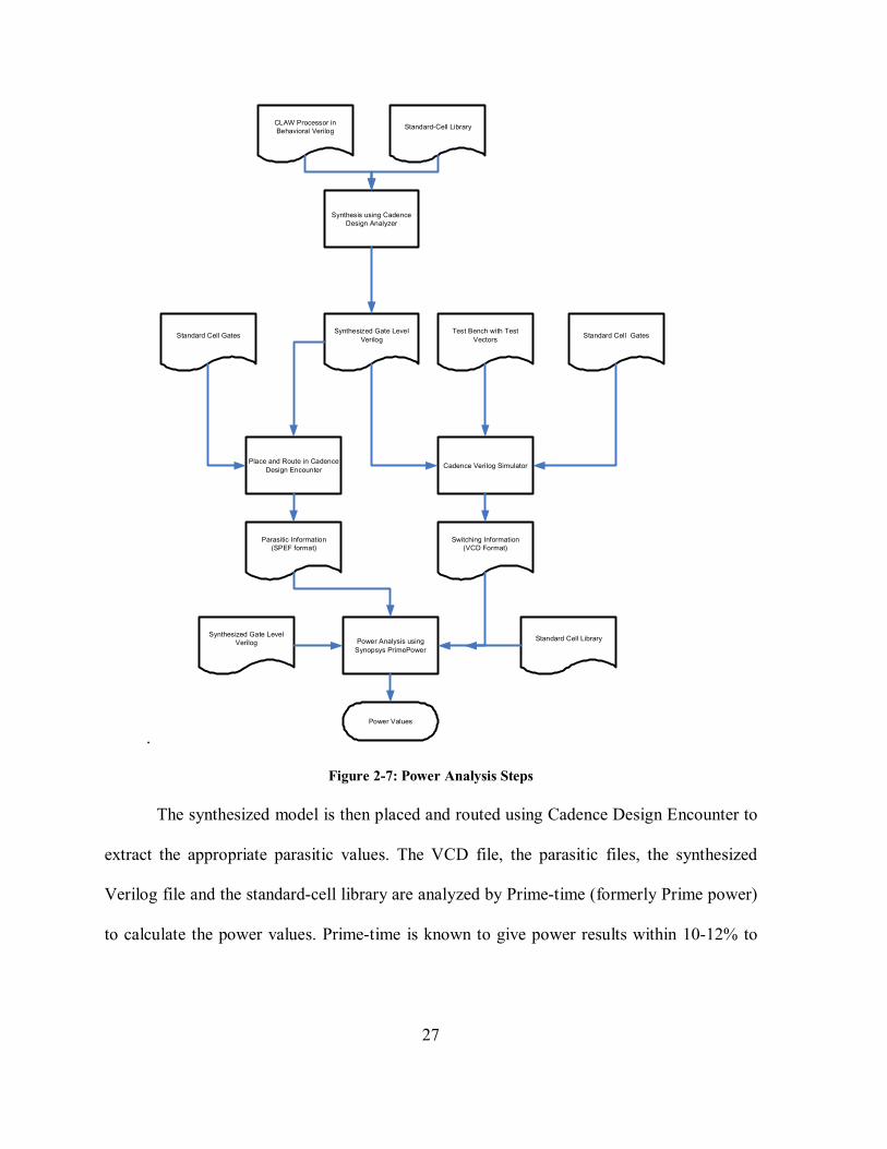
Figure 2-7 illustrates the steps to capture power values from the processor. First, we
take a behavioral model of the CLAW processor (written in Verilog), and synthesize it using
the Cadence design analyzer with 90nm Artisan SAGE-X Physical-IP RVT library. The
VDD for this library is 1V with 25°C operating temperature and typical operating conditions.
To simulate benchmarks on CLAW, we use the Verilog-XL simulation system. We
created a program that reads a CLAW executable file and extracts the text, read-only data
(rodata) and read-write data region. These information are saved in “text.txt” and “data.txt.”
During the fetch stage, the processor requests the appropriate instruction stored in the
appropriate location through the icpu_adr_i bus. The test-bench reads this address and
outputs the appropriate instruction from the text.txt through the icpu_dat_i bus. Similar
procedure is done for the data information when the processor encounters a load/store
instruction. This entire procedure is detailed in Figure 2-8. This step produces a VCD file
used for calculating switching in the processor-wires. The simulator also outputs the number
of clock-ticks required to simulate the benchmark.
27
.
Synthesis using Cadence Design Analyzer
CLAW Processor in Behavioral Verilog Standard-Cell Library
Synthesized Gate Level VerilogStandard Cell Gates Test Bench with Test
Vectors
Cadence Verilog SimulatorPlace and Route in Cadence Design Encounter
Power Analysis using Synopsys PrimePower
Parasitic Information (SPEF format)
Switching Information(VCD Format)
Power Values
Standard Cell Gates
Synthesized Gate Level Verilog Standard Cell Library
Figure 2-7: Power Analysis Steps
The synthesized model is then placed and routed using Cadence Design Encounter to
extract the appropriate parasitic values. The VCD file, the parasitic files, the synthesized
Verilog file and the standard-cell library are analyzed by Prime-time (formerly Prime power)
to calculate the power values. Prime-time is known to give power results within 10-12% to

28
the real system [53]. The power values with the simulation time from Verilog-XL can be
multiplied together to get the total energy
CLAW Executable
(ELF Format)ELF Extractor
.text section
Text.txt
.data section.rodata section
Data.txt
CLAW Test Bench
CLAW Synthesized
Verilog Processor
INSTRUCTION
DATA
PC
DATA ADDRESSDURING A LOAD/STORE
Figure 2-8: Running an Executable on CLAW

29
Chapter 3 Instruction-width optimization
It is known that all applications that are run on a system do not contain the same amount
of parallelism. Thus, one processor configuration cannot be used as a model for the optimal
energy and performance. Thus, there is a need for dynamically issue-width adaptive
processors. Large issue-width processors tend to introduce long wires which can increase
chip-power and decrease clock-frequency [60].
One promising approach is to divide certain components of a processor into smaller
chunks and place them close together. The components inside each chunk are connected by
fast links. The communication time between the chunks is relatively slow because the
distance is longer. This architecture is collectively called clustered architecture and each
“chunk” is called a cluster [40]. Traditionally, each cluster consists of a local register file and
a subset of function-units [50]. In order to gain the most optimum performance in a clustered
architecture, it is very important to keep the inter-cluster communication to a minimum [15]
[17] [22] [50].
The idea of clustered architecture has been used in superscalar processor for many years
[1] [17] [22]. Some VLIW DSP processors such as, TMS320C6x (by TI) [176], TigerSharc
(by Analog Devices) [166], Map 1000 (by Equator) have incorporated this implementation
[50]. VLIW architectures implement wide instruction words to allow issuing of multiple
instructions in software [38].
These architectures are inherently ideal for exploiting parallelism extracted by fine grain
compilers that analyze code beyond a basic block [8]. This gives VLIW machines a sufficient

30
large “window size” to look for ways to parallelize the code. A clustered VLIW processor
tries to please both the communication delay and achieve a high IPC all for a low cost [15].
In this work, we created a clustered VLIW architecture and provide a mechanism to
dynamically shutoff unwanted or unused clusters with the help of a profiler by inserting
specialized shutoff instructions. In the next sub-section, we discuss our methodology of
modifying the instruction width at run-time. Section 3.2 describes how the clock-controller
dynamically gate unwanted units. Section 3.3 explains the next-PC calculation
implementation for our processor. In 3.4, we show how the instruction-scheduler inserts this
specialized instruction. We present our results using EEMBC benchmarks in section 3.5, and
conclude this chapter in section 3.6.
3.1 Dynamic Issue-Width Scalability
CLAW is flexible-enough to be able to shutoff clusters at any level. For this work, we
study three-levels of cluster scalability: function-level, treegion-level and basic-block level.
Shutting-off and turning-on the clusters are both done using a “shutoff” instruction. The first
cluster must remain turned-on the whole time since it holds the stack, frame and return
address information.
Figure 3-1 illustrates the format of the shutoff instruction. The immediate field of this
instruction is a bit-vector that indicates which cluster has to be shutoff. For example, “shutoff
1111b” implies that cluster 1, 2, 3 and 4 must be shutoff, and the rest of the clusters (if
available) must be turned on. For the 32-bit ISA, up to 24 clusters can be controlled using
this shutoff instruction.

31
Figure 3-1: Shutoff Instruction Format
The “shutoff” instruction has to be the first instruction of the bundle and must be put in
an empty bundle, that is, the rest of the instructions in the bundle must be NOP. This
instruction is decoded by the fetch unit and the appropriate clusters are clock-gated. The rest
of the bundle is ignored and the next bundle is fetched.
3.2 Pipeline Clock-Gating In CLAW, the fetch unit partially decodes every instruction to see if a shutoff
instruction is fetched. If such an instruction is found, it then emits a signal to the clock-gating
unit to indicate that certain clusters need to be turned off (or turned on). In many previous
works, the clock gating is done only in a single stage. In some works such as [118] [97], they
suggest stalling the processor for ‘N’ cycles (where ‘N’ is the pipeline-depth) and issue a
broadcast to all the units. There are two major problems with this scenario. First, if the
number of shutoffs is not kept to a minimum, the processor stalls significant number of
times. Second, sending these broadcasts requires significant number of long wires, which can
potentially increase power.
To solve the two problems in the previous work, we created a cascaded clock-gating
circuit. Figure 3-2 shows the high-level block diagram of the clock gating circuit for a 4-
cluster CLAW processor. We implemented an override pin just in case the user does not want
to use the shutoff mechanism. There are three major components of our clock gating unit: the

32
simple-gating unit, the propagating unit and the latching unit. The simple-gating unit accepts
the clock as the input and simply calculates whether the clock must be gated or not. Figure
3-3 shows the block-diagram of the simple-gating unit.
FETC
H U
NIT
CLU
STE
R 1
CLU
STER
2C
LUST
ER 3
CLU
STER
4CLOCKGATING
UNIT
SHUTOFF SIGNALS
OVERRIDE
CLOCK
C3 CLK RR
MOP
C1 CLK EX
C1 CLK DECODE
C2 CLK RR
C2 CLK WB
C3 CLK DECODE
C3 CLK WB
C4 CLK WB
C4 CLK DECODE
C1 CLK WB
C2 CLK DECODE
C3 CLK EX
C4 CLK RR
C4 CLK EX
C2 CLK EX
C1 CLK RR
Figure 3-2: Overall Clock Gating Circuit Block Diagram
Figure 3-3: Clock Gating Logic

33
The propagating unit creates a cascaded clock-signal that is send to the next units. Each
of these clocks has a phase shift of 1 cycle that is fed into each of the stages of the processor.
The latching unit holds the clock gating information given by the fetch unit. This unit ensures
that any external interference does not affect the clock signal. The clock signals can be
changed only by fetch unit with the help of an enable signal. Figure 3-4 shows an example of
cascaded clock output for a 2 Cluster CLAW. At 30ns, the fetch unit is requesting that the
second cluster to be shutoff, and keep the rest of the clusters on. We can see that
“gated_clk_1[1]” shuts off immediately. This is being fed into the decode stage. The rest of
the gated clocks appear to mimic the same behavior as gated_clk_1 but with 1 cycle delay
from its predecessor. At 50ns, ‘0’ was found on the “shutoff_bits” bus, the clock signal did
not change because the enable (shutoff_en) was low.
Figure 3-4: Cascaded CLK Output
The advantage of such a clock-gating circuit is that it doesn’t disrupt any instructions
that are in the pipeline during the previous cycles. Also, there is only one Multi-Op
performance penalty to shutting off clusters. Such techniques have been presented for
clocking multi-cycle function units (e.g. [67]), but this is the first time it has been applied to

34
a general purpose processor. This complex clock-gating unit only increases the processor
area by 2.1% and did not cause any change in the frequency of the base-processor.
3.3 Next PC Calculation
For doing the appropriate next-PC calculations, we evaluated the different techniques
presented in section 1.1.5. Having a dedicated branch cluster for execution gives the
optimum performance compared to the other two schemes. Having a centralized scheme
seems to be the worst of all three. The branch replication scheme seems to add additional
complexity to the cluster and increase the dynamic code-size, which can have adverse effects
in terms of power consumption.
Some of the disadvantages of having a branch cluster are that the compiler must be
very capable in order to schedule all the branches to one certain cluster. Also, if we chose to
disable a certain number of clusters, the code might not perform as well as expected.
In CLAW ISA, when a jump instruction occurs, the return address register (r9) is
automatically written with address of the next MOP after the jump. On the other hand,
branches do not have any other implicit tasks. This helped us come up with a hybrid scheme
to handle control-transfer instructions. Branches could be executed in any clusters as
necessary. Jumps were all assigned to cluster 1. This mechanism helped reduce the possible
congestion that could happen in branch cluster. At the same time, an explicit instruction is
not necessary to write the return address into the return address register, thus reducing code-
size.

35
3.4 Instruction Scheduling and Shutoff Insertion
CLAW is a variable-width processor. The width can be varied with the feedback of the
architect, programmer and the user. In order to do this efficiently, we build such a processor
using a set of two issue clusters. In any clustered system, the biggest bottle-neck is the inter-
cluster communication. In order to reduce this effect, several scheduling algorithms have
been presented by previous researchers. We used the concept of scheduling the instructions
and assigning them in the same cycle called Unified-Assign and Schedule (UAS).
GCC provides several hooks that allow architects to manipulate and intercept the
ready-list at different stages of scheduling [39]. The UAS was attached to the
“TARGET_SCHED_FINISH_GLOBAL” hook. This hook is called immediately after the
treegions are created. Figure 3-5 shows the flow-diagram of the major steps involved in the
UAS implementation. A list of unscheduled RTL is taken from the Treegion scheduler and a
list of instructions that are ready in the current cycle is assembled. GCC does all the
scheduling at the RTL level. Fortunately, almost all RTL can be mapped 1-to-1 with the
CLAW OP in the machine description. Each instruction in this ready list is assigned to a
cluster is picked as per a priority function.
There are four different priority functions available in UAS, they are: sequential
placement, random placement, magnitude-weighted placement (MWP) and completion-
weighted placement (CWP). In sequential placement, the RTLs are assigned in a round-robin
fashion to each cluster. In Random placement, the RTLs are placed to a random cluster
chosen using a pseudo-random number generator (lrand48()). MWP schedules an RTL to the
same cluster as its predecessors. If the predecessors of the current RTL are assigned to two

36
different clusters, either one can be its target. In CWP, the RTL is assigned to the same
cluster as the predecessor that takes the longest to complete. The advantage CWP has over
MWP is that since the current RTL has to wait till the latest of its predecessor to complete,
the holes in between can be used to schedule a copy instruction. These priority functions
have a direct control over the performance and the energy consumption of the processor. We
show the results of all four priority functions in the results section. For more detailed
explanation about UAS, the reader is referred to [34].
LIST OF UNSCHEDULED OPS FROM TREEGION
SCHEDULER
READY LIST == NULL
READY_LIST = LIST OF OP READY IN CURRENT
CYCLE
X = HIGHEST PRIORITY OP FROM READY_LIST
PICK APPROPRIATE CLUSTER (C) IN WHICH X
CAN BE SCHEDULED
X SCHEDULABLE IN CLUSTER C ?
X = SCHEDULEDINSERT X IN
SCHEDULE_LIST WITH APPROPRIATE CLUSTER
INFO
NO
YES
C == NULL
NO
NO
INCREMENT CYCLE COUNT YES
YES
Figure 3-5: Design-Flow of UAS Algorithm on GCC
To make UAS more suitable for a length-adaptive processor, we slightly modified the
assignment-priority function. When an RTL can be assigned to multiple-clusters during
MWP and CWP scheme, the authors in [103] mention to randomly pick a cluster. We forced
our algorithm to choose cluster 1 (if it is an option) or a previously used cluster. This helped
us to potentially shutoff other clusters. Similarly, when a new cluster must be used, we again

37
forced our algorithm to choose cluster 1 or a cluster that has been used previously. This
helped us isolate unused clusters for a longer period of time to save energy.
An additional challenge was encountered in the register allocation phase. The register
allocator in GCC tries to minimize assigning instructions to different register classes by
mapping dependent-instructions into the same register class. Even though this can reduce
additional cluster-usage, the register-allocator does not take cycle-time into account. To
overcome this problem, the register allocator’s mapping function (reg_class(..) function in
passes.c [39]) was replaced with a specialized hook function (added using a new hook called
“TARGET_MACHINE_DEPENDENT_REG_CLASS”) that will assign instructions as per
the UAS scheduler. All the modifications described will not affect any other gcc port, and
our gcc source-code can be configured for any other gcc-backend (e.g. x86) and function
without any difficulty.
Initially, the compiler inserts a shutoff instruction with ‘0’ as its immediate field
(indicating all clusters must be on) at the beginning of the basic-block or the beginning of the
function. The unique ID of the shutoff RTLs are stored in a data-structure along with the
basic-block number in which it was inserted. The information is used by the profiler
(integrated into GCC as an additional pass) to know which shutoff instruction must be
updated.
The CLAW profiler is executed right before the instructions are output as a final stage
in GCC compiler. This is the final stage where the RTLs are visible and are not moved
between basic blocks. The profiler scans the static code provided by the compiler to see if
there are any empty clusters. Figure 3-6 shows an example of an empty cluster: if for the

38
duration of an entire basic-block (or function depending on the granularity) there exist a
common empty cluster, then the bit-vector for the appropriate shutoff instruction is updated.
Figure 3-6: Example of an Empty Cluster (marked in blue box)
Figure 3-7 shows the algorithm of our profiler to detect idle clusters to power-down
using the shutoff instruction for function-level and basic-block level shutoff insertion. Region
level shutoffs are a bit more complex and are detailed in section 3.5.2. The algorithm accepts
a block of instructions (BLK) as input. The profiler goes through every MOP to see if it can
find Cluster-Ops (COP) with only NOP, that is, an unused-cluster. If such a scenario is
noticed, the appropriate bit is set to ‘1’ in the ‘Unused’ array. M.count indicates the MOP
position in the BLK and C.count indicates COP position in the MOP M. This array is a two-
dimensional array with rows indicating the number of MOPs in the block (indicated by
BLK.MOP_Count) and the columns showing each cluster. This array must be dynamically
allocated, but it is not shown in the figure for simplicity.

39
Figure 3-7: Cluster-Shutoff Algorithm
After stepping through all the MOPs in BLK, the profiler goes through the ‘Unused’
array to find if all the MOPs have common clusters that can be shutoff. This is done by
checking if the summation of all the 1’s in a column is equal to the number of MOPs in BLK.
The list of empty clusters is returned back to the profiler from this function using the
“Shutoff_Cluster_List” variable. The profiler examines this to set the appropriate bit in the
shutoff instruction. The profiler also displays the number of cases where all the clusters are
turned-on for analysis.

40
3.5 Results
Sequential placement picks the appropriate target clusters in a round-robin fashion.
Random placement, assigns the instructions to the randomly chosen cluster. MWP assigns an
instruction to the same cluster as the instruction’s flow-dependent predecessors. In CWP
placement, the scheduler gives priority to the clusters that will be producing the instruction’s
operands relatively late in the schedule. CWP scans all the clusters which execute the
instructions that are dependent on the current instruction. The current instruction is assigned
to the cluster that produces its results the latest. The advantage of this scheme is that the copy
instructions are potentially easier to schedule without losing much cycle-time. In section we
show the base case results of all the CLAW configurations. This is then compared with the
different shutoff schemes mentioned in section 3.1
3.5.1 Base Results
Figure 3-8 shows the number of cycles required to execute these benchmarks in a 1-
cluster CLAW. Conven00 takes the longest number of cycles followed by dither, while ospf
seem to take the smallest. Figure 3-9, and Figure 3-10 shows the speed-up compared to one-
cluster for two-cluster and four-cluster CLAW machine. Routeloop is the most parallel
benchmark in the suite. Conven00 seem to be the least parallel of all the benchmarks.

41
0
100
200
300
400
500
600
aifir
f01
conv
en00
dith
er
ospf
puw
mod
rota
te
rout
eloo
kup
rspe
ed
ttspr
k01
vite
rb00
Mill
ions
Cycl
es
Figure 3-8: Execution-time for 1-Cluster CLAW
0
0.5
1
1.5
2
2.5
3
3.5
aifir
f01
conv
en00
dith
er
ospf
puw
mod
rota
te
rout
eloo
kup
rspe
ed
ttspr
k01
vite
rb00
Ave
rage
Sequential Random MWP CWP
Figure 3-9: Speedup of 2-Cluster CLAW over 1 Cluster Machine

42
0
0.5
1
1.5
2
2.5
3
3.5
aifir
f01
conv
en00
dith
er
ospf
puw
mod
rota
te
rout
eloo
kup
rspe
ed
ttspr
k01
vite
rb00
Ave
rage
Sequential Random MWP CWP
Figure 3-10: Speedup of 4 Cluster CLAW over 1 Cluster CLAW Machine
In a clustered architecture, it is necessary to keep the number of inter-cluster copy to a
minimum. Figure 3-11 and Figure 3-12 show the amount of copy instructions (in percentage)
in a two and four-cluster machine. CWP and MWP have virtually no copy instructions
(approximately 0.5% or less) when compared to random or sequential placement. These two
algorithms take the instructions and their dependencies into consideration, whereas random
and sequential placement, assigns the instructions ad-hoc.

43
0%
5%
10%
15%
20%
25%
30%
aifir
f01
conv
en00
dith
er
ospf
puw
mod
rota
te
rout
eloo
kup
rspe
ed
ttspr
k01
vite
rb00
Sequential Random MWP CWP
Figure 3-11: Percentage of Copy Instructions in 2-Cluster CLAW Machine
0%
5%
10%
15%
20%
25%
30%
aifir
f01
conv
en00
dith
er
ospf
puw
mod
rota
te
rout
eloo
kup
rspe
ed
ttspr
k01
vite
rb00
Sequential Random MWP CWP
Figure 3-12: Percentage of Copy Instructions for 4-Cluster CLAW Machine

44
The next step is to see the energy consumed by the benchmark for the different
CLAW machines with different number of clusters. Energy is used as a metric because it
takes into account the tightness of the schedule along with the average power consumption.
We believe that a processor that has slightly higher power dissipation, but executes a
program significantly faster is better than a processor that consumes less power while taking
longer to execute the same benchmark.
The static and dynamic energy values for a single cluster configuration are shown in
Figure 3-13. Figure 3-14 and Figure 3-15 show the dynamic energy values for two and four
cluster machine for the four placement types. OSPF is the smallest benchmark in the suite, so
it consumed the least energy. Conven00 is the largest benchmark in the set followed by
dither. Even though, ttsprk01 is the third-largest benchmark, it consumed ~30% more power
than conven00. Ttsprk01 contains more multiplication and division instructions than all the
benchmarks, and these two are power-intensive operations.
Sequential consumed the most energy since it has a significant amount of copy-
instructions. Similarly, MWP and CWP consumed the least amount of energy because it took
the benchmark into consideration during scheduling and emitted less copy instructions. The
energy consumption of MWP and CWP is identical in all the cases because, they both create
the same schedule for unit-latency instructions. In CLAW, all of the instructions, except the
MAC instructions, are unit latency instructions. MAC instructions are not output by the
compiler.
Figure 3-16 and Figure 3-17 show the static energy dissipation for 2-cluster and 4-
cluster CLAW, respectively. The static energy only contributes ~10-15% of the total energy

45
in all cases. The static energy also increased for 4-cluster CLAW since we have a larger area
and a higher potential for idle wires.
0
50
100
150
200
250
300
aifir
f01
conv
en00
dith
er
ospf
puw
mod
rota
te
rout
eloo
kup
rspe
ed
ttspr
k01
vite
rb00
mill
iJou
les
Dynamic Energy Static Energy
Figure 3-13: Dynamic and Static Energy or 1 Cluster CLAW

46
0
50
100
150
200
250
300
aifir
f01
conv
en00
dith
er
ospf
puw
mod
rota
te
rout
eloo
kup
rspe
ed
ttspr
k01
vite
rb00
mill
iJou
les
Sequential Random MWP CWP
Figure 3-14: Dynamic Energy Values for a 2-Cluster CLAW Processor
0
50
100
150
200
250
300
aifir
f01
conv
en00
dith
er
ospf
puw
mod
rota
te
rout
eloo
kup
rspe
ed
ttspr
k01
vite
rb00
mill
ijoul
es
Sequential Random MWP CWP
Figure 3-15: Dynamic Energy Values for a 4-Cluster CLAW Processor

47
05
1015202530354045
aifir
f01
conv
en00
dith
er
ospf
puw
mod
rota
te
rout
eloo
kup
rspe
ed
ttspr
k01
vite
rb00
mill
iJou
les
Sequential Random MWP CWP
Figure 3-16: Static Energy Values for 2-Cluster CLAW Processor
05
1015202530354045
aifir
f01
conv
en00
dith
er
ospf
puw
mod
rota
te
rout
eloo
kup
rspe
ed
ttspr
k01
vite
rb00
mill
iJou
les
Sequential Random MWP CWP
Figure 3-17: Static Energy Values for 4-Cluster CLAW Processor
3.5.2 Dynamic Length-Adaptivity
To study the energy savings by shutting off unused clusters, we inserted shutoff
instructions at the basic-block level and the function level for 2-Cluster and 4-Cluster

48
configuration of the CLAW processor. Figure 3-18 shows the dynamic energy distribution
for 2 and 4 cluster CLAW. For ease of comparison, we also plotted the base values of the
energy values taken from Figure 3-14 through Figure 3-17. ‘
For the 2-Cluster CLAW, there is no dynamic energy difference at all. The profiler
did not find any significant opportunities to shutoff any clusters. For the 4 cluster CLAW,
majority of the programs only used 2 clusters, this helped shutoff the other 2 clusters
majority of the time, and thus save energy. Inserting the shutoff at the function-level did not
increase the code size significantly (< 0.1%). This did not cause any energy increase.
0
50
100
150
200
250
aifir
f01
conv
en00
dith
er
ospf
puw
mod
rota
te
rout
eloo
kup
rspe
ed
ttspr
k01
vite
rb00
2 Cluster CLAW Base 2 Cluster CLAW With Cluster Shutoff4 Cluster CLAW Base 4 Cluster CLAW After Cluster Shutoff
Figure 3-18: Dynamic Energy Distribution Function-Level Shutoff Insertion
The static energy distribution is shown in Figure 3-19. Since it is impossible to
physically shutoff flip-flops in a HDL based design, we have also provided the static power
differences as a data-label for all the static energy graphs from this point forward. The static
energy difference is within the threshold of the error-rate of Primetime. The main reason why

49
we compared static-energy values is to see if the shutoff insertion blew up the static value.
For 2-Cluster CLAW the values barely changed. This again is due to the fact that the profiler
was unable to find any clusters to shutoff. For the 4 Cluster CLAW, two of the clusters were
shutoff for many of the benchmarks. This caused some idle wires, but this did not cause any
significant change. The static power for 2-cluster CLAW barely produced any change,
whereas a 7% increase was found in the 4-cluster processor. This increase translated to 0.7%
total-power increase. Please note that an asterisk (*) indicates a change that is between -0.5%
and 0.5%
*******
*
**
*
6%9%
9%
9%
3%
4%
9%
4%
1%4%
7%
0
50
100
150
200
250
aifir
f01
conv
en00
dith
er
ospf
puw
mod
rota
te
rout
eloo
kup
rspe
ed
ttspr
k01
vite
rb00
Ave
rage
Mill
ijoul
es
2 Cluster CLAW Base 2 Cluster CLAW With Cluster Shutoff4 Cluster CLAW Base 4 Cluster CLAW After Cluster Shutoff
Figure 3-19: Static Energy Distribution Function-Level Shutoff Insertion
Next, we looked at the dynamic energy distribution when the shutoff instruction was
inserted on the basic block (BB) level. Figure 3-20 shows our results. For the 2-Cluster case,
almost all the benchmarks did poorly. This is because, inserting a shutoff instruction at every
basic block level created a code-explosion. Recall that the shutoff OP is placed in a separate

50
MOP with no other useful instructions. Our benchmarks, on average had 2-3 MOP per basic-
block. If the compiler was able to pack more instructions into each basic block, then we
could have achieved a better result. For 4 Cluster CLAW, similar code explosion did occur.
This code-explosion is overshadowed by the fact that almost always two of the four clusters
is always shutoff. This energy savings helped hide many of code-explosion problems.
0
50
100
150
200
250
300
aifir
f01
conv
en00
dith
er
ospf
puw
mod
rota
te
rout
eloo
kup
rspe
ed
ttspr
k01
vite
rb00
Mill
ijoul
es
2 Cluster CLAW Base 2 Cluster CLAW With Cluster Shutoff4 Cluster CLAW Base 4 Cluster CLAW With Cluster Shutoff
Figure 3-20: Dynamic Energy Distribution BB-Level Shutoff Insertion
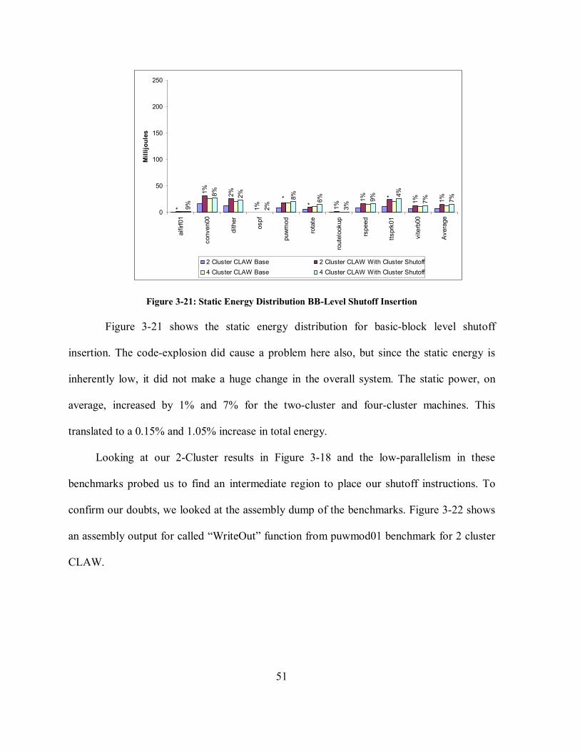
51
1%1%
*1%
1%
*
*
1%
2%1%
*
7%7%
4%
9%
3%
6%8%
2%
2%8%
9%
0
50
100
150
200
250
aifir
f01
conv
en00
dith
er
ospf
puw
mod
rota
te
rout
eloo
kup
rspe
ed
ttspr
k01
vite
rb00
Ave
rage
Mill
ijoul
es
2 Cluster CLAW Base 2 Cluster CLAW With Cluster Shutoff4 Cluster CLAW Base 4 Cluster CLAW With Cluster Shutoff
Figure 3-21: Static Energy Distribution BB-Level Shutoff Insertion
Figure 3-21 shows the static energy distribution for basic-block level shutoff
insertion. The code-explosion did cause a problem here also, but since the static energy is
inherently low, it did not make a huge change in the overall system. The static power, on
average, increased by 1% and 7% for the two-cluster and four-cluster machines. This
translated to a 0.15% and 1.05% increase in total energy.
Looking at our 2-Cluster results in Figure 3-18 and the low-parallelism in these
benchmarks probed us to find an intermediate region to place our shutoff instructions. To
confirm our doubts, we looked at the assembly dump of the benchmarks. Figure 3-22 shows
an assembly output for called “WriteOut” function from puwmod01 benchmark for 2 cluster
CLAW.

52
Figure 3-22: WriteOut function from Puwmod01
Figure 3-23 shows the control-flow graph and cluster usage of each basic block. GCC
puts the prologue and epilogue of each benchmark in a separate basic block and they are not
available for scheduling with other blocks. Thus, we have indicated them in as a separate
block with different color. We can see that only one of the five blocks is using two clusters.
When we insert the shutoffs at the function level, we are unable to shutoff any of the clusters
due to the effects of block 2. Similarly, if we insert shutoffs at the basic-block level, we have
added 5 extra MOP into the system which contributes to greater cycle-time.

53
BLOCK 1(CLUSTER USAGE: 1)
BLOCK 2 (CLUSTER USAGE: 1, 2
BLOCK 5(CLUSTER USAGE: 1)
BLOCK 4(CLUSTER USAGE: 1)
BLOCK 3(CLUSTER USAGE: 1)
Figure 3-23: Control Flow Graph of WriteOut
Treegions is a collection of basic blocks that have the same entry point and different
exit points. Figure 3-24 shows the control flow graph using treegions of the same program.
We investigated the possibility of inserting shutoffs at the head of each treegion to see if this
gave us an energy reduction. In our example function, we asked the processor to shutoff none
of the clusters at the head of treegion 1 and asked cluster 2 to be turned off during the
execution of treegions 2. It is important to note that a small trivial function is used in this
example to illustrate our idea. Such optimization is really geared for more complex functions
with treegions containing large number of basic-blocks.

54
BLOCK 1(CLUSTER USAGE: 1)
TREEGION 1
BLOCK 2 AND 3(CLUSTER USAGE: 1, 2)
BLOCK 5(CLUSTER USAGE: 1)
TREEGION 2
BLOCK 4(CLUSTER USAGE: 1)
Figure 3-24: CFG using Treegions in WriteOut
We made another interesting observation about cluster usage and treegions. Figure
3-25 shows the CFG of treegions from the from the “ZTableLookup” function of ttsprk01
program, compiled for 4-Cluster CLAW. The prologue and epilogue are indicated in yellow
because it was not included in the scheduling. We can see that all treegions have the same
cluster usage. So, inserting a shutoff that performs the same operation at the head of every
basic block can be redundant. Thus, we created an extra step in our optimizer that will step
through all the treegions and remove any redundant shutoff instructions.

55
Treegion 1(Cluster Usage: 1)
Treegion 2(Cluster Usage: 1)
Treegion 3(Cluster Usage: 1)
Treegion 4(Cluster Usage: 1)
Treegion 5(Cluster Usage: 1)
Treegion 6(Cluster Usage: 1)
EPILOGUE
PROLOGUE
Figure 3-25: CFG using Treegions for ZtableLookup in Ttsprk01
Inserting shutoffs at the function-level and basic-block level were trivial compared to
inserting them at the treegion-level. To get the information about each treegions, we created
several new data-structures to convey this information from the treegion-scheduler to the
profiler. Figure 3-26 shows the algorithm that calculates cluster usage for each treegion.

56
Figure 3-26: Calculating Cluster Usage for Each Region In the first loop, we go through each RTL and extract its destination and source
registers. This information is used by the “Calculate_Cluster_Usage” function to calculate
the cluster usage of this RTL. For example, an RTL whose destination register is in Cluster 2
and source register in cluster 1 signifies that the instruction is using both cluster 1 and cluster
2. Each RTL is uniquely defined by a number called “Instruction Unique Identification
Number (UID).” This number remains unchanged for the lifetime of the function. We created
a new data-structure to hold the cluster-usage information of the RTL indexed by the UID.
Second, we go through every basic-block in the function and find all the instructions
inside each basic block. We find the cluster-usage of each RTL inside the basic block from
the above-mentioned data-structure and “OR” them together to get the cluster-usage of the

57
whole basic-block. Finally, we look at all the blocks inside a treegion, and then “OR” all of
their usage to gather the cluster-usage for each region.
Next, we insert the shutoff RTL at all the head-node of each treegions. Figure 3-27
shows the algorithm used for this process. At first, we walk through all the RTL in the
function. When we find a basic-block head, we record its number and region in which it is
located. If this is a head-node, then we insert a shutoff RTL here. As mentioned in the
previous section that shutoff instruction contains an immediate value which is a bit-vector
that tells which clusters must be shutoff.
Figure 3-27: Shutoff Insertion at Treegion-level algorithm
Using the algorithm in Figure 3-26, we computed the usage of each treegion. The
shutoff instruction requires the complement of this value. To compute this, we create a bit-
vector for the number of clusters available in the system, and then exclusive-OR that value
with the region-usage to get which clusters must be shutoff. This information is set as the
immediate value of the shutoff RTL and then it is inserted into the RTL-list.

58
We illustrated using an example in Figure 3-25 that there are cases were a treegion
and its predecessors all have the same usage. Thus, there is no need to have another shutoff
inserted after the predecessor. To remove such redundant shutoffs, we implemented the
algorithm illustrated in Figure 3-28.
Figure 3-28: Redundant Shutoff Removal Algorithm This algorithm first goes through all the treegions in the program and finds the head
basic-block. If the block does not have any predecessors, indicating that it is the first block of
the program, then the delete flag for this region (implemented as a array of Boolean values),
is set to false. If the block contains predecessors, then we initially assume we do not need this
shutoff RTL. Then the algorithm steps through all the predecessors of this block to see which
region they fall in. If any of these treegions have a different cluster usage than the current
block, then we set the delete-flag to false. The region-list is walked-through from the top-
down to recursively remove all the redundant shutoffs in the program.
In the algorithms shown in Figure 3-26, Figure 3-27 and Figure 3-28, we did not
explicitly use the word “treegion,” even though we used them for treegions. This is because

59
they are not treegion-specific. If the architect wishes to insert shutoff instructions at a
different region-granularity (e.g. Superblocks), these algorithms can be used. We
demonstrated our work on a treegion scheduler because UAS is tightly-coupled with a
treegion-scheduler.
Figure 3-29 shows our dynamic energy values for 2 and 4-cluster CLAW when the
shutoffs were inserted at the treegion level and after removing the redundant shutoffs. For the
4-Cluster CLAW, inserting them at the region-level (with redundant shutoff removal) seems
to have gotten results very close to the function-level shutoffs. This is because for 4-Cluster
CLAW, the last 2 clusters seem to be idle most of the time. So inserting the shutoffs at the
function-level helps to gain good results without any code-explosion. For the 2 Cluster
CLAW, function-level seem to give no improvement, but when we inserts shutoffs at the
region level, the profiler was able to find holes in the system to give some energy reduction.
With the redundant shutoff removal, too much unnecessary shutoffs were not inserted, thus
reducing code-size.
For highly-parallel benchmarks such as route lookup, the region-level shutoff insertion
achieved 9% energy reduction. For benchmarks with low-parallelism such as conven00 we
achieved a dynamic-energy reduction of 29%. On average, we were able to gain a 17%
energy reduction. Figure 3-30 shows the static energy distribution for the region-level shutoff
insertion. Static power, on average, increased by 1% and 7% for the two-cluster and 4-cluster
processor configurations. This translated to 0.15% and 1.05% of the total power change in
the processor. Static energy did not increase considerably. For the 4-Cluster CLAW, it is
very comparable to the function-level shutoff insertion. For 2-Cluster configuration, the static

60
energy contributed on average, 1% increase in the total energy, but it is definitely was
shadowed by the dynamic-energy decrease.
0
50
100
150
200
250
aifir
f01
conv
en00
dith
er
ospf
puw
mod
rota
te
rout
eloo
kup
rspe
ed
ttspr
k01
vite
rb00
Mill
ijoul
es
2 Cluster CLAW Base 2 Cluster CLAW With Cluster Shutoff
4 Cluster CLAW Base 4 Cluster CLAW After Cluster Shutoff
Figure 3-29: Dynamic Energy Consumption for Region-Level Shutoff
*
* 1%
*
* * * * 1% * 1%7%
6% 2%
5%
7% 4%
3%
9% 9%
9% 7%
0
50
100
150
200
250
aifir
f01
conv
en00
dith
er
ospf
puw
mod
rota
te
rout
eloo
kup
rspe
ed
ttspr
k01
vite
rb00
Ave
rage
Mill
ijoul
es
2 Cluster CLAW Base 2 Cluster CLAW With Cluster Shutoff4 Cluster CLAW Base 4 Cluster CLAW After Cluster Shutoff
Figure 3-30: Static Energy Consumption with Region-level Shutoff

61
To provide a fair comparison with the treegion-level shutoff insertion with redundant
shutoff insertion, we inserted the shutoff operations at the basic block level and the applied
our redundant shutoff removal algorithm. Figure 3-31and Figure 3-32 shows the dynamic
and static energy distribution. For the 4-cluster implementation, the dynamic energy
reduction was very much comparable with the treegion-level insertion. For the 2-cluster
implementation, the treegion level was able to give, on average 10% more energy reduction
across the benchmarks. This is because basic-blocks in GCC are small and some adjacent
ones had different cluster utilization. Thus, a new MOP (with shutoff operation) had to be
inserted at the head of several basic block and the overhead incurred for shutting off and
turning on the clusters contributed to this increase. The static power increase was as same as
treegion-level shutoff, but the static energy increased a little due to the increase in code-size.
0
50
100
150
200
250
aifir
f01
conv
en00
dith
er
ospf
puw
mod
rota
te
rout
eloo
kup
rspe
ed
ttspr
k01
vite
rb00
Ave
rage
Mill
ijoul
es
2 Cluster CLAW Base 2 Cluster CLAW With Cluster Shutoff4 Cluster CLAW Base 4 Cluster CLAW After Cluster Shutoff
Figure 3-31: Dynamic Energy Consumption with BB-level Shutoff with Redundant Shutoff Removal

62
1%*1%****
*
**
1%
7%7%
4%9%
3%
5%7%
2%
2%7%
8%
0
50
100
150
200
250
aifir
f01
conv
en00
dith
er
ospf
puw
mod
rota
te
rout
eloo
kup
rspe
ed
ttspr
k01
vite
rb00
Ave
rage
Mill
ijoul
es
2 Cluster CLAW Base 2 Cluster CLAW With Cluster Shutoff4 Cluster CLAW Base 4 Cluster CLAW After Cluster Shutoff
Figure 3-32: Static Energy Consumption with BB-level Shutoff with Redundant Shutoff Removal
3.6 Conclusion
In this section, we presented a dynamically-scalable clustered general purpose
processor. The processor-width was dictated by the compiler using a specialized instruction
to shutoff unused data-paths. We also presented a compiler-framework that is able to pack-
instructions into clusters and isolate unused clusters. The results were demonstrated using
EEMBC benchmarks.
We found that when the processor was over-designed for the application, simple
techniques such as function-level shutoffs is enough to achieve good energy reduction. When
this is not the case, a complex scheme such as a region-level shutoff scheme must be
implemented. The region-level scheme tried to keep the code-size from exploding yet

63
provided a mechanism to squeeze out as much energy as possible from the processor.

64
Chapter 4 Opcode Optimization
Instruction decoding is one of the essential steps in most traditional processors. It is
known that a decoder can consume up to 10% of the total power and energy inside a
processor [13]. A compiler (along with the assembler) is responsible for generating the
instructions that are fed into a decoder. For example, if a compiler (or assembler) is not able
to output an increment instruction, then the decoder will rarely have a chance to decode such
instructions. It is also known that a compiler tends to output certain instructions more than
others. In our experiments, we found add-immediate to be one of the most frequently
generated instructions.
Switching on a wire or port is the main cause of power dissipation. If we are able to
reduce switching between two adjacent events in a wire, then we are able save power and
energy. The Hamming distance is a simple yet powerful way to calculate the number of bit-
switches between two instructions. The Hamming distance between two instructions is found
by applying an XOR operation between two instructions and counting the resulting number
of set bits.
One possible way to reduce the switching activity is to schedule instructions that have
low hamming distance close to each other. This approach is not always possible and can
potentially degrade performance. Another solution is to find the instructions that are close to
each other and modify their opcodes such that the switching is reduced. Although modifying
the opcodes at run-time inside a processor is impossible, profiling a representative

65
application and designing the opcodes appropriately can help reduce power dissipation and
energy consumption.
Table 4-1 shows two instructions from the aifirf01 benchmark that is encoded using the
original (CLAW) opcode. Table 4-2 shows our modification to the opcode (the opcode
modification is indicated in bold font). It is trivial to see that by a simple opcode-
reassignment, we are able to reduce hamming distance from 13 to 12.
Table 4-1: Original CLAW Encoding Instruction Assembled Output
1. l.movhi r17,0x107 1a 20 01 07
2. l.movlo r17, 0x9d50 2a 31 9d 50
Hamming Distance 13
Table 4-2: Encoded to Reduce Hamming Distance Instruction Assembled Output
1. l.movhi r17,0x107 1a 20 01 07
2. l.movlo r17, 0x9d50 3a 31 9d 50
Hamming Distance 12
In the next subsection, we explain the popular ways to encode instructions in today’s
embedded processors. Section 4.2 explains our opcode optimization algorithm in detail. In
section 4.3 we show the results of the optimization. We conclude this section in section 4.5.

66
4.1 Popular ISA Encoding in Existing Embedded Systems
A common approach to encoding instructions, especially in RISC architectures is
called telescoping encoding [142]. This trend is followed by many embedded processor
architectures such as MIPS [108] and Atmel [167].
In telescoping encoding, two similar instructions of same type (e.g. Arithmetic
instructions) have the same primary opcode, and different secondary opcodes. There are two
approaches to decode instructions for such encoding: parallel or serial approach. Figure 4-1
and Figure 4-2 show how to decode an OR instruction using these approaches.
4 BITS6 BITS
2 BITS
CONCATENATE
12 BITS12 BITS1101 1100 0100
YES/NO
COMPARATOR
Figure 4-1: Parallel Approach to Decode an OR instruction
In the parallel approach, the opcode and sub-opcodes are compared in a single step. To
decode an OR instruction, the parallel approach takes 12 comparisons, regardless of a match.
In the serial approach, the primary opcode is compared, then if there is a match, the

67
secondary opcode is compared. Such cascaded comparisons can introduce additional latches
into the system
Suppose that there are 1 million OR instructions in a benchmark. If the decoder is
written using a parallel approach, then to decode this instruction, there must be 12x1 million
comparisons. In the serial approach, in addition to 12x1 million comparisons, 6x1 million
additional latches are charged and discharged, which can consume significant amount of
energy.
4 BITS
6 BITS
2 BITS
CONCATENATE
6 BITS6 BITS00 0100
COMPARATOR
6 BITS
11 0111
YES/NO
VDD GND
GND
COMPARATOR
YES / NO Figure 4-2: Serial Approach to Decode OR instruction
Not all instructions have multiple fields. For example, the “return from exception (rfe)”
instruction does not have a sub-opcode field. The unused bits in this instruction are left as
“don’t-cares.” An alarming observation is that many instructions that occur commonly in
several benchmarks have sub-opcode fields and instructions that rarely occur in a regular
program execution have no sub-opcode field. This can have a significant impact on energy.

68
4.2 Methodology
In order to understand the code generated by the compiler, we took one application
(aifir01) as a training set and ran through our high-level CLAW simulator. Aifir01 is referred
to as the training benchmark, and the rest of the benchmarks are called the testing
benchmarks. We were surprised to see that the trace only had 70% coverage of the entire
ISA. After examining the machine description of the compiler, we found that only 80-85% of
the instructions in the ISA are represented. To see the general trend, we also examined the
GCC machine description of ARM and ATMEL. Similar percentage of coverage was seen in
the base machine description of these processors.
We were unable to create machine description to represent instructions such as
pipeline-synchronization. Similarly, there are some set of instructions that are used for
exception handling. It is known that exceptions happen rarely in a typical system, thus these
instructions are rarely executed when compared to all other instructions. But for all of the
above mentioned architectures, decoding of these rare instructions is straightforward and the
instructions that are commonly used have multiple-opcode fields, which can consume
additional time and power to decode.
To extract the instruction trace of the training benchmarks, a CLAW instruction-set
simulator was written in C++. To find adjacent instructions, Markov chains were created
from the instruction trace. In the beginning, two, three and four-instruction chains were
considered, but the three and four-instruction chains contributed minimally, thus we do not
discuss them in detail in this paper.

69
To create the optimal opcode-distribution, the traces are analyzed using the algorithm
described in Figure 4-3. The function accepts the instruction-trace of the training benchmark
and a list of instructions the compiler is able to represent in its machine description.
Figure 4-3: Opcode Optimization Algorithm
This trace is then stepped through by another function that creates another list to hold
all the instructions that the current trace is able to represent. It holds all the instructions in
descending value of the instruction-type occurrence. This list is usually a subset of the GCC
represented traces.

70
The instruction trace, along with the two lists, is fed into another function to prioritize
the opcodes. For example, if “ADD” is the highest occurring instruction in the training list,
then the priority transmitter will try and make sure the ADD instruction gets a unique
primary opcode and no sub-opcode.
When all the elements of the “Trace_Rep_Insns” list is visited, the optimizer visits all
the instructions that GCC is able to represent, not found in “Trace_Rep_Insns.” The rest of
instructions in the ISA are given primary and secondary opcode fields. This function outputs
the “Prio_Insn_Trace.”
Next, the Prio_Insn_Trace is analyzed to make sure adjacent instructions have the
lowest switching. This adjacent-instruction chain along with the “Prio_Insn_Trace” is sent to
a minimum-distance genetic algorithm similar to [128] that minimizes switching among the
adjacent instructions. This function gives an instruction template that contains information
about the placement of various components of the instruction.
This template is used to remap the instructions from the original CLAW encoding to
the new optimized encoding. Similarly, this template is used to remap all testing benchmark
to the newly optimized encoding. Figure 4-4 gives a flow-diagram for designing a new
opcode and how a new benchmark is remapped using the template of the new opcode
configuration.
Some operations such as addition, multiplication, bitwise operations, etc. are
commutative. In Table 4-3, we can see that when we switch register r2 in the second
instruction, we were able to reduce the total hamming distance between two instructions by
one.

71
CLAWBENCHMARKEXECUTABLE CLAW
SIMULATOR
START ADDRESS
INSTRUCTION TRACE
OPCODE OPTIMIZATION ALGORITHM
NEW OPCODES
STOP ADDRESS
OPCODEREMAPPER
CLAW DECODER GENERATOR
(ctrl.v)
ANY CLAW BENCHMARK EXECUTABLE
B.EXE
REMAPPED EXECUTABLE
(B.EXE)
TRAINING BENCHMARK
TESTING BENCHMARK
Figure 4-4: Flow-Diagram of our Methodology
Table 4-3: Illustration of Distance Saved using Source Register Switching Instruction Assembled Inst. First l.add r15,r13,r2 e1 f0 10 00 Second l.add r14,r2, r12 e1 a2 60 00 Hamming Distance 5 First l.add r15,r13,r2 e1 f0 10 00 Second (Switched) l.add r14,r12,r2 e1 ac 10 00 Hamming Distance 4
After profiling our benchmarks for possible register switching, we found that the
compiler, about 97-99% of the time (in all benchmarks), matched the source registers of the
instructions whenever possible. That is, it automatically performed the process explained in
table 4. We found very few cases where this was not true. Creating a stage in our analyzer to
do this did not cause any notable reduction in the energy consumption.
4.3 Results
The energy consumption was first measured for the single-cluster CLAW processor.
The entire benchmark was executed through the Verilog code. Even though, this method took
significant amount of time and resources, this was the only non-biased way to prove the

72
accuracy of these techniques. Figure 4-5 shows the obtained base values for leakage and
dynamic energy.
In all benchmarks, static/leakage energy is approximately 10-15% of the dynamic
energy. Even-though static or leakage energy is considered a dominating factor in submicron
transistor sizes, their dominance is mainly in the caches and RAM, not in the processor core
[77]. Only the processor core was simulated, so static energy effects are low. Second, the
libraries we are using are regular VT (RVT) libraries. It has been proven in [116] that these
libraries are very low-leakage libraries. RVT libraries are suggested by ITRS as the most
suitable library for designing embedded systems.
Figure 4-5: Base Energy Values for the Benchmarks
It can be inferred from Figure 4-5 that the ospf benchmark consumed the least energy
and ttsprk01 consumed the most energy. This is because ospf is the smallest benchmark with

73
2.3 million instructions. Conven00 is the largest benchmark in the set followed by dither.
Even though, ttsprk01 is the third-largest benchmark, it consumed ~30% more power than
conven00. Ttsprk01 contains more multiplication and division computations than all the
benchmarks, and these two units are power-intensive.
Each of the ten benchmarks are at one point used as a training benchmark. Then each
of the benchmark was tested on all the trained processors. The results are indicated in Table
4-4 and
Table 4-5. The benchmark on the horizontal axis is the training benchmark for the
genetic algorithm. A positive difference indicates a reduction in energy and a negative
difference indicates an increase in energy consumption. The highlighted fields show cases
were the training and testing benchmarks are the same. An asterisk was used to indicate a
change between -0.5% and 0.5%
Table 4-4: Percentage Dynamic Energy Reduction Aifirf01 Conven00 Dither Ospf Puwmod Rotate Routelkup Rspeed Ttsprk Viterb
Aifirf01 16% 1% 10% 14% * * 1% 3% 1% 1%
Conven00 2% 16% -1% 3% 2% * 2% 5% 5% 2%
Dither 4% 7% 16% * 3% 11% * 9% -1% -2%
Ospf 16% * 2% 19% 1% * * 4% * 2%
Puwmod 10% -2% 15% * 17% * 9% 12% 9% -6%
Rotate 6% * 11% 3% 8% 14% * 8% * *
Routelkup 2% * 4% 3% 4% 4% 14% 4% 4% *
Rspeed 4% 3% 2% 2% 4% 2% 6% 13% 4% 4%
Ttsprk01 7% 3% * * 1% -1% -1% -1% 9% -3%
Viterb00 -2% -1% -2% -4% -2% -2% -4% -2% -2% 16%

74
Table 4-5: Percentage Static Energy Reduction
Aifirf01 Conven00 Dither Ospf Puwmod Rotate Routelkup Rspeed Ttsprk Viterb
Aifirf01 * 1% * -1% -4% -2% * * * 1%
Conven00 7% 8% 8% 8% 8% 8% 8% 8% 8% 8%
Dither 2% 2% 2% 2% 2% 2% 2% 2% 2% 2%
Ospf -3% -3% -3% -3% -2% -2% -2% -2% -2% -2%
Puwmod -1% * -1% -1% -1% -1% -1% -1% -1% -1%
Rotate 6% 7% 7% 7% 7% 7% 7% 7% 7% 7%
Routelkup 7% 9% 9% 8% 8% 8% 8% 8% 8% 8%
Rspeed 4% * * -1% * * * * * *
Ttsprk01 -10% -1% -1% -1% -2% -2% -2% * -3% -2%
Viterb00 1% * * 2% * * * 2% 2% -1%
The first question that arose in our minds after looking at Table 4-4 is that since it is
well known that a decoder only contributes 10% of the total CPU energy, then how can an
energy reduction as high as 19% be seen in the trained CPU? To understand this question, the
timing diagram of the processor was examined at each stage namely: fetch, decode, register-
read, execute and write-back. Also other components of the processor such as the freeze unit
(also used to forward data between pipelines), store-buffer, ALU, memory-unit, multiply and
divide unit, and the exception handler were studied. Several debug runs were done with
$display statements to capture the bit-activity in the major buses inside the CPU components.
For the OSPF-optimized decoder, the processor achieved a 19% energy reduction for
OPSF. Figure 4-6 shows a pie chart that categorizes the major energy-saving contributors.
The decoder contributed for 11% of the 19% energy savings in OSPF. The fetch-unit
provided 3.5% and the instruction-busses and the other intermediate units provided for 2.5%

75
of the 19% savings. The exception unit and the freeze-unit (also called stall-unit) provided
for 1% each. This trend was followed by all the benchmarks.
Decoder, 11%
Freeze Unit, 1%
Exception Unit, 1%
Fetch Unit, 3.50%
Buses and Other Units, 2.50%
Figure 4-6: Dynamic Energy Savings in Each Unit of OSPF
To understand more about the characteristics of the benchmark a study of the
structure of the high-level C code was performed. Figure 4-7 shows the number of function-
calls that each of the benchmarks encounter during their execution. Function-calls are
important because during each function-call all registers used by the callee are saved on the
stack and then restored from the stack in the beginning and the termination of each call.

76
Number of Function Calls made by EEMBC Benchmark
0
2000
4000
6000
8000
10000
12000
14000
16000
aifir
f01
conv
en00
dith
er
ospf
puw
mod
rota
te
rout
eloo
kup
rspe
ed
ttspr
k01
vite
rb00
Num
ber o
f Fun
ctio
n Ca
lls
Figure 4-7: Dynamic Function-calls in Each Benchmark
In CLAW assembly, the only method to implement push and pop information into the
stack is by using a load-word or store-word to access the stack. After all loads or stores the
stack pointer (register r1) is incremented or decremented accordingly using an add-
immediate instruction, creating a common instruction chain for benchmarks high in stack
operations. When the dynamic trace of aifir01 was observed, there were a significant amount
of memory operations, which matches the results showing a high number of function calls.
Therefore, optimizing on the instruction chain for stack operations greatly reduces energy for
aifir01. Also, the benchmark calls a function called “GetInputValues” which loads a
significant amount of data from a global variable (inpVariableROM). To load from a global
variable, the 16 least significant bits of the variable are moved using the “movlo” instruction.
Then the 16 most significant bits are loaded into the register using a “movhi” instruction that

77
loads its immediate value into the top 16 bits of a register. “Movhi” and “movlo” instructions
are analogous to the movw and movt instruction in the ARM architecture.
Dither and rotate operate on an image. Unlike aifir01, they do not refetch the image
every iteration. Instead, all necessary images are stored in a large array before the
“th_signal_start ()” function. Thus, they have significantly less function-calls than aifir01,
and therefore they do not benefit as much from the stack chain optimization. However, these
two benchmarks skip around inside an image, thus they have significant amount of branches
when compared to the other benchmarks. This explains why the optimized decoder for these
benchmarks performs well when executing the other benchmark.
It is popularly known that viterbi decoding is used to decode conventional codes in
communication systems. It is also well known that both convolutional encoding (conven00)
and viterbi decoders (viterb00) have a significant amount of shifts, adds and memory
operations. However, as per Table 4-4, an instruction-set that is optimized for one fails to
give a significant energy reduction on the other. Examining the instruction trace and the
high-level code reveals that conven00 performed all computations on 4-byte and 1 byte data
widths, that is, they had variables and data that were either “int” or “char.” Viterb00 did all
its computations on 2-byte data-width (“short”). CLAW has different instructions for each
data-size. Table 4-6 shows an example of loads for the 3 different data-set.
Thus, when trained using viterb00, most of the half-word instructions were given
smaller opcodes and the word-level and byte-level ones were given longer opcodes. The
opposite was done for conven00.

78
Table 4-6: Different Load Instruction Types in CLAW Data Type Load Inst. Meaning 1-Byte l.lbs Load data & sign-extend it to 1 byte-width 1-Byte l.lbz Load data & zero-extend it to 1 byte-width 2-Bytes l.lhs Load data & sign-extend it to 2-byte width 2-Bytes l.lhz Load data & zero-extend it to 2-byte width 4-Bytes l.lws Load data & sign-extend it to 4-byte width 4-Bytes l.lwz Load data & zero-extend it to 4-byte width
A further study to understand the results are to examine the number of instructions
required to meet the 50% coverage displayed Figure 4-8. This result indicates the diversity in
the benchmark. For example, ospf requires only 4 chains to get 50% coverage; this implies
that if another benchmark contains some of these chains then a good energy reduction can be
seen. Aifir01 and ospf have 2 chains in common that falls in this range. Thus, a high dynamic
energy reduction can be seen in ospf when the opcodes are optimized for aifir01.
Number of Chains Required to get a 50% Coverage in EEMBC Benchmarks
0
2
4
6
8
10
12
14
16
aifirf0
1
conv
en00
dithe
ros
pf
puwmod
rotate
routeloo
kup
rspee
d
ttsprk
01
viterb
00
Figure 4-8: Number of Distinct Instruction Chains achieving 50% coverage

79
Both puwmod and rspeed were very computationally intensive. Even though, rspeed
had significantly more function-calls than puwmod, the dominating chains for both of them
were instructions such as add, rotate, extend etc. In these two benchmarks, chain-count was
distributed evenly among its chains. Therefore, it was hard to optimize for these benchmarks.
The advantage of such algorithms with several distinct chains is that they give some energy
reduction for most of the training set. Finally, routelookup also exhibited similar behavior.
But it had a lot more distinct chains than puwmod or rspeed. Thus, it was even harder to
analyze them and find an optimal opcode-encoding.
Many of the explanations thus far in this section apply primarily to dynamic energy.
Sub-threshold leakage is a dominating issue only in the memory hierarchy [77]. For this
work, memory was not modeled since it was unable to find a synthesizable memory that can
be interfaced with the CLAW Verilog core. Figure 4-5 shows that in CLAW, leakage energy,
on average, contribute only 10-15% of the total energy consumption. It can be seen from
Table 4-5 that leakage-energy tends to increase slightly when there some decrease in
dynamic-energy. This is because the primary way to reduce dynamic energy is to reduce
switching in the processor interconnects, which tends to give slight increase in leakage
energy. After further analysis of individual components of the processor, the increase in
leakage energy was in components where switching is greatly reduced: the decoder and the
instruction busses.

80
4.4 Multi-cluster CLAW Configurations
The next step is to see if our algorithm can be applied to processors with larger issue-width. For this work, we choose to apply our algorithm on the benchmarks compiled (using CWP as the priority scheme)
for the 2-Cluster and 4-Cluster CLAW machines. Table 4-7 shows the dynamic energy savings, and Table 4-8 shows the static energy savings. Table 4-9 and Table 4-10 show the
dynamic and static energy savings for 4-Cluster CLAW. These values are compared with the
base-values shown in Figure 3-14, Figure 3-15, Figure 3-16 and Figure 3-17. Most of the
results scaled with the processor issue-width. There were a few changes (within 1%) when
we went from 1-Cluster to 2-Cluster, but going from 2-Cluster to 4-Cluster there is virtually
no change.
We can see that for all the benchmarks except Routelookup, the results scaled pretty
well. This is because most of the benchmarks do not have a very high parallelism, so the
same instructions that were adjacent in 1-cluster were more or less adjacent in the 2-Cluster
and 4-Cluster CLAW. Routelookup is the most parallel benchmark in our set, so its results
gave small difference. Secondly, even though we change the issue-width, the benchmark
remains the same. For example, let’s say a benchmark in the 1-cluster executable had 1000
addition operations. This number does not change when we go to a 4-Cluster machine.
Similarly, with the exception of copy operations, the instruction-types will also
remain the same. CWP does a good job avoiding copies, so this instruction does not
contribute heavily in the executable. Since the dynamic energy did not change much, the
static energy trends also remained the same.
Table 4-7: Percentage Dynamic Energy Reduction ( 2 Cluster CLAW) Aifirf01 Conven00 Dither Ospf Puwmod Rotate Routelkup Rspeed Ttsprk Viterb

81
Aifirf01 14% 1% 10% 14% * * 1% 3% 1% 1%
Conven00 2% 15% -1% 3% 2% * 3% 5% 5% 2%
Dither 3% 7% 16% * 3% 11% 1% 9% -1% -2%
Ospf 16% * 2% 19% 1% * * 4% * 2%
Puwmod 10% -2% 14% * 17% * 9% 12% 9% -6%
Rotate 6% * 11% 3% 7% 14% * 8% * *
Routelkup 2% * 4% 4% 4% 4% 14% 3% 4% *
Rspeed 4% 3% 2% 2% 4% 2% 4% 13% 4% 4%
Ttsprk01 7% 3% * * 1% -1% -1% -1% 9% -3%
Viterb00 -2% -1% -2% -4% -2% -1% -4% -2% -2% 15%
Table 4-8: Percentage Static Energy Reduction (2 Cluster CLAW)
Aifirf01 Conven00 Dither Ospf Puwmod Rotate Routelkup Rspeed Ttsprk Viterb
Aifirf01 * 1% * -1% -4% -2% * * * 1%
Conven00 7% 8% 8% 8% 8% 8% 8% 8% 8% 8%
Dither 2% 2% 2% 2% 2% 2% 2% 2% 2% 2%
Ospf -3% -3% -3% -3% -2% -2% -2% -2% -2% -2%
Puwmod -1% * -1% -1% -1% -1% -1% -1% -1% -1%
Rotate 6% 7% 7% 7% 7% 7% 7% 7% 7% 7%
Routelkup 7% 9% 9% 8% 8% 8% 8% 8% 8% 8%
Rspeed 4% * * -1% * * * * * *
Ttsprk01 -10% -1% -1% -1% -2% -2% -2% * -3% -2%
Viterb00 1% * * 2% * * * 2% 2% -1%
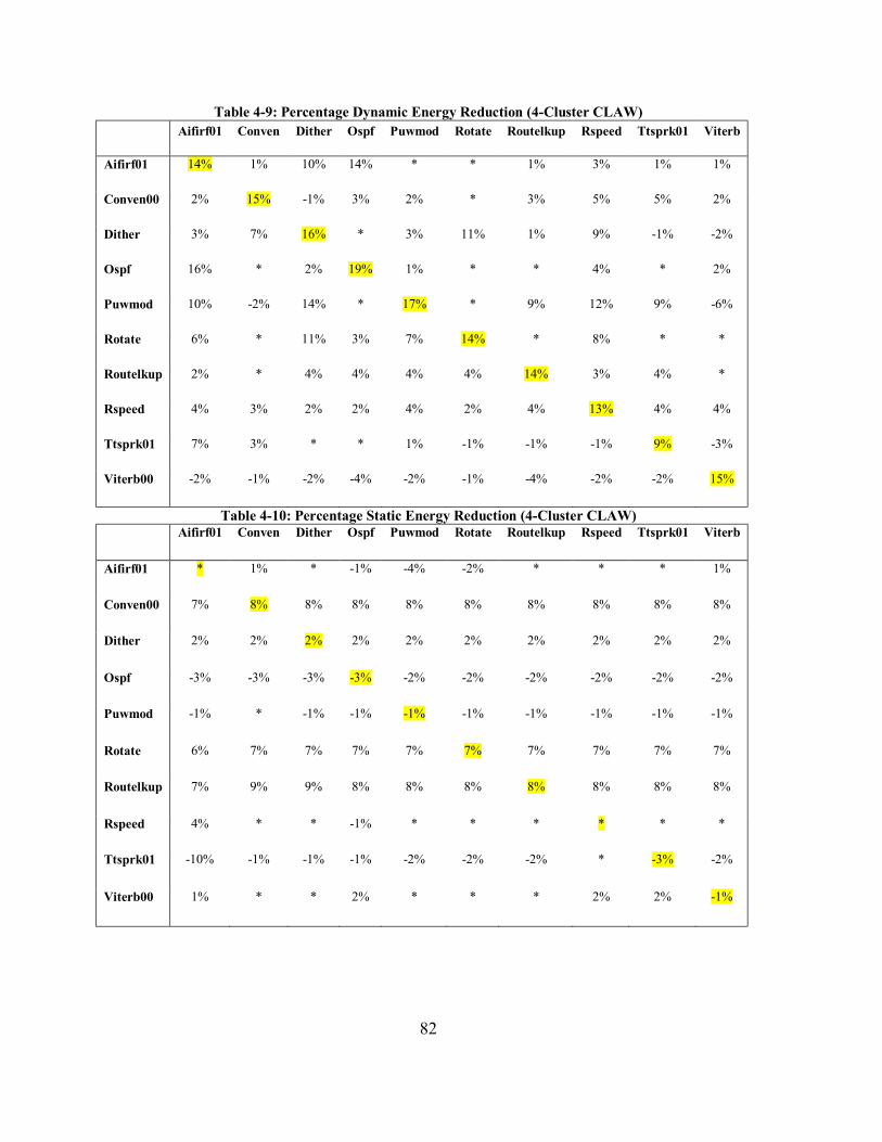
82
Table 4-9: Percentage Dynamic Energy Reduction (4-Cluster CLAW) Aifirf01 Conven Dither Ospf Puwmod Rotate Routelkup Rspeed Ttsprk01 Viterb
Aifirf01 14% 1% 10% 14% * * 1% 3% 1% 1%
Conven00 2% 15% -1% 3% 2% * 3% 5% 5% 2%
Dither 3% 7% 16% * 3% 11% 1% 9% -1% -2%
Ospf 16% * 2% 19% 1% * * 4% * 2%
Puwmod 10% -2% 14% * 17% * 9% 12% 9% -6%
Rotate 6% * 11% 3% 7% 14% * 8% * *
Routelkup 2% * 4% 4% 4% 4% 14% 3% 4% *
Rspeed 4% 3% 2% 2% 4% 2% 4% 13% 4% 4%
Ttsprk01 7% 3% * * 1% -1% -1% -1% 9% -3%
Viterb00 -2% -1% -2% -4% -2% -1% -4% -2% -2% 15%
Table 4-10: Percentage Static Energy Reduction (4-Cluster CLAW) Aifirf01 Conven Dither Ospf Puwmod Rotate Routelkup Rspeed Ttsprk01 Viterb
Aifirf01 * 1% * -1% -4% -2% * * * 1%
Conven00 7% 8% 8% 8% 8% 8% 8% 8% 8% 8%
Dither 2% 2% 2% 2% 2% 2% 2% 2% 2% 2%
Ospf -3% -3% -3% -3% -2% -2% -2% -2% -2% -2%
Puwmod -1% * -1% -1% -1% -1% -1% -1% -1% -1%
Rotate 6% 7% 7% 7% 7% 7% 7% 7% 7% 7%
Routelkup 7% 9% 9% 8% 8% 8% 8% 8% 8% 8%
Rspeed 4% * * -1% * * * * * *
Ttsprk01 -10% -1% -1% -1% -2% -2% -2% * -3% -2%
Viterb00 1% * * 2% * * * 2% 2% -1%

83
4.5 Conclusion
In this chapter, a technique to optimize the instruction-set based on a sample of the
workload for which the processor is designed is presented. The presented technique neither
causes any additional cycle-count nor increase the clock period of the base processor. The
only major hardware modification that is necessary is the instruction decoder. The newly
generated instruction-decoder can be swapped with the original without any further
modifications to the processor. We demonstrated this algorithm on 1-Cluster, 2-Cluster and
4-Cluster CLAW. We showed that results scaled as we increase the cluster-sizes.
This chapter shows that if the sample set is selected correctly, some energy reduction is
achieved by intelligently assigning opcodes and no performance is lost. When the training
and the testing application were the same, we achieved an average 17.2% energy reduction.
When the testing application and training application were different, a 9.4% energy reduction
was achieved. In addition, this technique also provides a loose-rubric to design software for
the particular processor. If the new software that is to be added to the system is designed in a
similar structure and contains similar characteristics (e.g. memory intensive vs.
computationally intensive or word-length vs. byte-length), there can be an energy reduction
with no performance loss.

84
Chapter 5 Register-Sharing
Registers play a significant role in improving the instruction-level-parallelism (ILP) in
modern systems [11] [55] [150]. Large register-files, with the help of an optimal register
allocation scheme, can greatly reduce the amount of spill-code inserted in the program [8].
This can in turn reduce the memory traffic, thus reducing the number of execution cycles
necessary for the application.
To remove false dependences in dynamically scheduled processors, designers implement
rename map tables that match the architectural registers to physical registers [10] [13]. In
statically scheduled systems, these false dependencies are resolved by using tighter register
allocation schemes and/or a large register-file. In either case, there can be a huge amount of
pressure exerted on register-file [11].
Even though the idea of implementing large register-file is attractive for performance,
there can be setbacks in terms of energy or power dissipation, access time and chip area
[115]. It is known that register-file power dissipation accounts for about 10-20% of the
overall power dissipation [11] [55]. For example, in the Motorola M.CORE architecture, the
register-file energy consumption accounts for 16% of the total processor power and 42% of
the dual-path power [13].

85
5.1 Preliminary Analysis
To benefit from register sharing, it is necessary to see if there is a large amount of
duplicate values in the register-file. Table 5-1 shows the percent of zero and duplicate writes
in a register-file from for different architectures with different register-file sizes.
It is apparent that there are a large number of duplicated values stored inside a register-
file. Therefore we investigated if a certain value was written repeatedly. Our analysis found
that ‘0’ was written at a greater frequency than any other values. It can be seen from Table
5-1 that there is a significant amount of zeros written into registers.
Table 5-1: Zero and Duplicate writes for different register file configurations ARM (Thumb Mode) 1-Cluster CLAW Simplescalar 2.0 IA-64 (Soft Float) IA-64 (Hard Float)
Benchmark Zero-Write
Dupl. Write Zero-Write
Dupl. Write Zero-Write
Dupl. Write
Zero-Write
Dupl. Write
Zero-Write
Dupl. Write
aifirf01 24% 43% 13% 46% 20% 67% 1% 5% 1% 5% conven00 15% 48% 30% 49% 25% 48% 1% 7% 1% 7% dither 8% 14% 8% 21% 10% 15% 2% 10% 2% 10% puwmod 3% 25% 6% 39% 3% 30% 1% 9% 1% 10% rotate 3% 17% 3% 23% 3% 17% 1% 10% 1% 11% routelkup 5% 40% 7% 53% 5% 44% 1% 5% 1% 5% rspeed01 4% 20% 21% 45% 3% 23% 1% 7% 1% 7% ttsprk01 5% 28% 25% 53% 3% 39% 1% 8% 1% 8% viterbi 11% 31% 12% 40% 7% 42% 1% 6% 1% 6% ospf 6% 35% 19% 41% 3% 32% 1% 5% 1% 5%
5.2 Register Sharing Techniques
It is apparent from section 1.1.2 that power dissipation of the register-file is a highly
researched area. It is also visible that many register optimization techniques can greatly help
in improving the performance of the program. There are several different register sharing
techniques proposed in research in works such as [150] and [10]. In this investigation, we
pick two classes of register sharing structures: register map table [10] [150] and a register
map-vector [150]. Figure 5-1 explains the top-level block diagram of these two structures.

86
Figure 5-1: Top-level block diagram of the map-table/map-vector
A register map-table is used to map certain architectural registers to other registers
that hold the certain values. As mentioned in section 5.1, there is a significant amount of ‘0’
values written into the register-file. We choose one architectural register (r0) that is
permanently set to zero, and any register whose value is zero is mapped to r0. The primary
advantage of this scheme is that we do not access the register-file for zero-writes. Secondly,
register pressure is potentially reduced.
The second approach is to use a map-vector to indicate which registers hold the zero
value. Each register is assigned a bit in the vector to indicate if its result is zero. If the
corresponding bit is set, then the register-file is not accessed. In our experiments, the map-
vector generally consumed about 30-40% less power than a map-table. As soon as we reach
the write-back stage, we know the register value along with the result to be written. If the
value written is zero then a bit is set in a map-table and the register-file is not accessed.
Otherwise the value is forwarded to the register-file and is written to the appropriate register.
To explain this further, we present a flowchart for these stages in Figure 5-2 and Figure 5-3.

87
Figure 5-2: Flow-Diagram for the Writeback Stage
Figure 5-3: Flow-diagram of the Register-Read Stage

88
5.3 Experiments and Terminology
To accurately portray register writes, we created synthetic-benchmarks with 1-million
register writes and 2-million register reads. Synthetic benchmarks were used to filter out
unwanted bias and to keep the study generic. It can be verified that similar trends can be
achieved by using commercial benchmarks. In each run, we increased the number of zeros by
a certain percentage. Throughout this paper, the number of zeros in the stream is given in
terms of percentage. It is worth mentioning that we only read registers that have already been
written (with the exception of the stack pointer and the return value register). We explain our
different writing schemes in Figure 5-4. Please note that in the figure, the number of writes
was reduced to 20 for the ease of explanation.
We also created sequences of zero writes into the register-file. These sequences of
writes are placed in different regions of the trace. For example a sequence 40-10 implies that
the first 10% of the register writes are non-zero values and the next 40% of the writes are
zeros. The remaining 50% of the values are non-zero writes. We take this model further and
break the zero sequence into intervals to see their effects. For example, for the experiment
40-40-10 implies that the first 40% (bold) of the writes are non-zeros, and then in the next
60%, the 40% zeros (underlined) are divided into intervals of 10%. In the next section we
explain the results of these distributions.

89
Figure 5-4: Different Placements of Zero-Writes
5.4 Results
To understand the impact of the register-file size on power dissipation, we modeled a 32-bit
register-file of size 16, 32, 64, 128 and 256 registers. The percentage of zero-writes
(distributed randomly) is varied from 0-100% in intervals of 5%. Figure 5-5 to Figure 5-9
displays our findings.
In all cases, using a register-file with a map-table consumed more power than only
the register-file without any value sharing. We call this the “base” case. The map-vector
gives a power advantage when we have 20% and 45% of zeroes for the register-file size of
16 and 32, respectively. The map vector fails to provide a power-reduction for the 128 and
256 sized register-file. This is because the internal power of the cell dominates the overall

90
power consumption for a larger register-file. For 64 entry file, the break-even point lies after
95%.
0.01
0.011
0.012
0.013
0.014
0.015
0.016
0.017
0.018
0 5 10 15 20 25 30 35 40 45 50 55 60 65 70 75 80 85 90 95 100
Percentage zero-writes
Pow
er(W
)
Base Map Vector Map Table
Figure 5-5: Power Dissipation for Random Register-Write (Reg. File Size = 16)
0.015
0.017
0.019
0.021
0.023
0.025
0.027
0.029
0.031
0 5 10 15 20 25 30 35 40 45 50 55 60 65 70 75 80 85 90 95 100
Percentage of Zero-Writes
Pow
er(W
)
Base Map Vector Map Table
Figure 5-6: Power Dissipation for Random Register-Write (Reg. File Size = 32)

91
Next, we wanted to study the impact of register zero-write in sequences (seq.) placed
at different parts of the trace. We investigated for the most beneficial section of the trace to
schedule a chunk of zero-writes. The zero-writes were inserted at 10%, 40% and 80% of the
trace. The segment size was modeled from 10-80%, whenever applicable. Since the map-
table failed to provide any power reduction for the overall system, we do not investigate its
effects any further.
0.037
0.039
0.041
0.043
0.045
0.047
0.049
0.051
0.053
0 5 10 15 20 25 30 35 40 45 50 55 60 65 70 75 80 85 90 95 100
Percentage Zero Writes
Pow
er(W
)
Base Map Vector Map Table
Figure 5-7: Power Dissipation for random Register-Write (Reg. File Size = 64)

92
0.072
0.074
0.076
0.078
0.08
0.082
0.084
0.086
0.088
0.09
0 5 10 15 20 25 30 35 40 45 50 55 60 65 70 75 80 85 90 95 100
Percentage Zero Writes
Pow
er(W
)
Base Map Vector Map Table
Figure 5-8: Power Dissipation for random Register-Write (Reg. File Size = 128)
0.14
0.145
0.15
0.155
0.16
0.165
0.17
0 5 10 15 20 25 30 35 40 45 50 55 60 65 70 75 80 85 90 95 100
Percentage Zero Writes
Pow
er(W
)
Base Map Vector Map Table
Figure 5-9: Power Dissipation for random Register-Write (Reg. File Size = 256)

93
It can be seen from Figure 5-10 through Figure 5-14 that a slight power reduction is
achieved when zeros are placed in the beginning. This is due to a reduced amount of
switching in the ports and inside the registers, since everything is initialized to zero in the
beginning.
Now, we extend our previous results and divide these sequences into interval chains
(seq-int). For a given program, the compiler will typically be able to distribute five, 2% zero-
write chains more easily than a single 10% chain. The values of the intervals were chosen to
be 2%, 5%, and 10% respectively. These values were chosen because 2, 5 and 10 are
common divisors of 10, 40 and 80, thus allowing the results to be a fair comparison. Figure
5-15 through Figure 5-19 shows our results.
0
0.002
0.004
0.006
0.008
0.01
0.012
0.014
0.016
0.018
10--1
010
--20
10--3
010
--40
10--6
010
--80
40--1
040
--20
40--3
040
--40
40--5
080
--10
80--2
0
Sequence (Percent Zero -- Location)
Pow
er(W
)
Base Map Vector
Figure 5-10: Power Dissipation for Sequential Writes (Reg. File Size = 16)

94
0
0.005
0.01
0.015
0.02
0.025
0.03
10--1
010
--20
10--3
010
--40
10--6
010
--80
40--1
040
--20
40--3
040
--40
40--5
080
--10
80--2
0
Sequence (Percent Zero -- Location)
Pow
er (W
)
Base Map Vector
Figure 5-11: Power Dissipation for Sequential Writes (Reg. File Size = 32)
0.036
0.038
0.04
0.042
0.044
0.046
0.048
10--1
010
--20
10--3
010
--40
10--6
010
--80
40--1
040
--20
40--3
040
--40
40--5
080
--10
80--2
0
Sequence (Percent Zeros -- Location)
Pow
er(W
)
Base Map Vector
Figure 5-12: Power Dissipation for Sequential Writes (Reg. File Size = 64)

95
In the sequence interval distribution, the power dissipation for all cases is slightly
larger than the sequence case but lower than the random placement. The segment size did not
create a significant reduction in the power consumption. This is because the dynamic power
saved by the chunks did not offset the internal power, unlike the sequence placement. For a
large register-file, the internal power dominated, thus making the savings from these
techniques insignificant. When split into intervals, the starting placement did not cause any
major changes to the power reduction. We believe this is also due to the domination of the
internal power.
0.068
0.07
0.072
0.074
0.076
0.078
0.08
0.082
0.084
0.086
0.088
10--10
10--20
10--30
10--4
010
--60
10--8
040--1
040
--20
40--3
040
--40
40--50
80--10
80--2
0
Sequence (Percent Zeros -- Location)
Pow
er(W
)
Base Map Vector
Figure 5-13: Power Dissipation for Sequential Writes (Reg. File Size = 128)

96
0.135
0.14
0.145
0.15
0.155
0.16
0.165
10--1
010
--20
10--3
010
--40
10--6
010
--80
40--1
040
--20
40--3
040
--40
40--5
080
--10
80--2
0
Sequence (Percent Zeros -- Location)
Pow
er(W
)
Base Map Vector
Figure 5-14: Power Dissipation for Sequential Writes (Reg. File Size = 256)
0
0.002
0.004
0.006
0.008
0.01
0.012
0.014
0.016
10--1
0--2
10--1
0--5
10--1
0--10
10--4
0--2
10--4
0--5
10--4
0--10
10--8
0--2
10--8
0--5
10--8
0--10
40--1
0--2
40--1
0--5
40--1
0--10
40--4
0--2
40--4
0--5
40--4
0--10
80--1
0--2
80--1
0--5
80--1
0--10
Seq. Intervals (Pct Zeros -- Placement -- Seq. length)
Pow
er (W
)
Base Map Vector
Figure 5-15: Power Dissipation for Seq-int writes (Reg. File Size = 16)

97
0.0195
0.02
0.0205
0.021
0.0215
0.022
0.0225
0.023
10--1
0--2
10--1
0--5
10--1
0--10
10--4
0--2
10--4
0--5
10--4
0--10
10--8
0--2
10--8
0--5
10--8
0--10
40--1
0--2
40--1
0--5
40--1
0--10
40--4
0--2
40--4
0--5
40--4
0--10
80--1
0--2
80--1
0--5
80--1
0--10
Seq. Intervals (Pct Zero--Placement Pct -- Seq. Length)
Pow
er(W
)
32 Registers Base 32 Registers Map Vector
Figure 5-16: Power Dissipation for Seq-int writes (Reg. File Size = 32)
0.036
0.037
0.038
0.039
0.04
0.041
0.042
0.043
0.044
0.045
0.046
10--1
0--2
10--1
0--5
10--1
0--10
10--4
0--2
10--4
0--5
10--4
0--10
10--8
0--2
10--8
0--5
10--8
0--10
40--1
0--2
40--1
0--5
40--1
0--10
40--4
0--2
40--4
0--5
40--4
0--10
80--1
0--2
80--1
0--5
80--1
0--10
Seq. Intervals (Pct Zero--Placement Pct. -- Seq Length)
Pow
er(W
)
64 Registers Base 64 Registers Map Vector
Figure 5-17: Power Dissipation for Seq-int writes (Reg. File Size = 64)

98
0.073
0.074
0.075
0.076
0.077
0.078
0.079
0.08
0.081
10--10--2
10--10--5
10--1
0--10
10--4
0--2
10--4
0--5
10--4
0--10
10--8
0--2
10--8
0--5
10--80--1
0
40--1
0--2
40--10--5
40--1
0--10
40--4
0--2
40--4
0--5
40--4
0--10
80--10--2
80--1
0--5
80--1
0--10
Seq. Intervals (Pct Zero -- Placement Pct. -- Seq. length)
Pow
er(W
)
128 Registers Base 128 Registers Map Vector
Figure 5-18: Power Dissipation for Seq-int writes (Reg. File Size = 128)
0.135
0.14
0.145
0.15
0.155
0.16
0.165
10--1
0--2
10--1
0--5
10--1
0--10
10--4
0--2
10--4
0--5
10--4
0--10
10--8
0--2
10--8
0--5
10--8
0--10
40--1
0--2
40--1
0--5
40--1
0--10
40--4
0--2
40--4
0--5
40--4
0--10
80--1
0--2
80--1
0--5
80--1
0--10
Seq. Intervals (Pct Zero -- Placement Pct. -- Seq. Length)
Pow
er(W
)
256 Registers Base 256 Registers Map Vector
Figure 5-19: Power Dissipation for Seq-int writes (Reg. File Size = 256)

99
5.5 Conclusion
This study reveals several power dissipation patterns of the register-file. Adding these
structures can cause a power reduction only when there is a significant amount of zero-writes
present in the workload. Similarly, scheduling multiple zero-writes together, regardless of
the destination register, can give some power reduction for small register-file. Some power-
reduction can also be achieved if it is able to divide the common-value writes into intervals
than just placing them at random. It is best to make register-sharing structures configurable
so that the user can turn them off when they feel there isn’t enough common-value to provide
any power-benefit.
These techniques can be extended to a physical or an architectural register-file. The
impact of zero-writes on power dissipation can be useful in several ways. For example, a
compiler can use this information and schedule instructions that potentially have a zero-write
together and form chunks. In addition, the processor can gate a map-vector so that the
compiler or profiler can predict and communicate that the number of zero-write in the system
is low.
100
Chapter 6 A Case study on IEEE 802.11n PHY
6.1 Motivation
CLAW is an ideal processor for embedded systems that support diverse, complex
applications. CLAW is capable of understanding this diversity inside an application and is
able minimize the overall energy required to execute the application. To find an ideal niche
for the CLAW processor, we explored new algorithms that fit these properties.
Communications, especially Wireless Local Area Networks (WLAN) is one of the
most developing fields today [110] [156] [144]. Most of the WLAN today use some flavor of
IEEE 802.11 standard [156] [110]. The previous standard, IEEE 802.11g operates at the
20MHz bandwidth. With the necessity of higher throughput and data-rates, IEEE
Communication society set up an IEEE 802.11 High-Throughput Study Group (HTSG) to
come up with a new standard for WLAN transmission [156], called IEEE 802.11n. A final
version of this standard is projected to be completed by November 2009.
One of the major findings of HTSG is the short comings of the current 802.11
Physical layer. They proposed a new multiple-input, multiple-output (MIMO) WLAN
scheme that is able to provide high throughput and data-rate. At present a third-draft of the
IEEE 802.11n standard is proposed [170].
One of the main advantages of high data-rate WLAN is that it makes
telecommunication systems more nomadic [110]. Many such nomadic systems use batteries
as the sole energy-source. Thus, reducing energy consumption is one of the compulsory

101
requirements for such systems. To date, there has not been a single study that characterizes
the energy consumption of such systems using 802.11n.
In this chapter, we provide a model for the IEEE 802.11n transmitter and receiver, as
per the parameters mentioned in [170], using the C language. We implement these units
strictly per the standard and using the advice given by IEEE 802.11 experts in [144] [157]
[102] [3]. The authors of [102] have provided parameters for all the major components in
this standard to achieve the best performance and data-rate. They demonstrate using detailed
simulations that using certain parameters for the components can help achieve high data-rate.
These parameters are used in our algorithm. We then characterize these two units and
measure the energy consumed. Finally, we show how a dynamic length-adaptive processor
can provide an energy benefit without losing performance for the transmitter and receiver.
In the next section, we explain the individual components of the transmitter and
receiver. In Section 6.3, we show how the components are assembled to create a non-biased
model. We display our results in section 6.4 and conclude this chapter in section 6.5.
6.2 IEEE 802.11n Architecture
Figure 6-1 and Figure 6-2 shows the major components of the transmitter and receiver.
There are seven major components for the transmitter: forward-error correction transmitter
(FEC), interleaver, OFDM symbol mapper, MIMO transmitter, the inverse fast Fourier
transform (IFFT), and the digital to analog converter. The receiver complements the work of
the transmitter using these six components: analog to digital converter, fast Fourier-transform
(FFT), MIMO decoder, OFDM symbol demapper, de-interleaver and FEC decoder. In this

102
work, we maintain all our work in the digital side, thus we do not model the analog to digital
or digital to analog conversion. In the next sub-sections, each of these components is
explained in detail.
FORWARD ERROR CORRECTION
ENCODER
INTERLEAVER
OFDM SYMBOL MAPPER
MIMO ENCODER
ANTENNA SELECTOR IFFTIFFT
DIGITAL TO ANALOG CONVERTER
DIGITAL TO ANALOG CONVERTER
DATA FROM THEMAC UNIT
Figure 6-1: IEEE 802.11N Transmitter

103
ANALOG TO DIGITAL CONVERTER
ANALOG TO DIGITAL CONVERTER FFTFFT MIMO DECODER
OFDM SYMBOL DE-MAPPER
DE-INTERLEAVER
FORWARD ERROR CORRECTION
DECODER
BIT-STREAM TOMAC UNIT
Figure 6-2: IEEE 802.11N Receiver
6.2.1 FEC Transmitter and Decoder
Forward-error control is a system of error control, whereby the sender adds redundant
bits into the stream called error correction code. These code can be used to correct any errors
occurred during transmission of data though the channel. As per the past research, LDPC or
Convolutional Encoding can be used for FEC in IEEE 802.11N. For best performance,
authors of [102] advise the use of convolutional encoding. Figure 6-3 shows the block-
diagram of a convolutional transmitter. The incoming data is brought into the constraint
register one bit at a time and the output bits are generated by modulo-2 addition of the
required bits from the constraint register. As per their experiments, the best results can be

104
achieved when the convolutional transmitter has a constraint length (K) of 7, and using the
generator polynomials 91 (1138) and 121 (1718).
Figure 6-3: Convolutional Transmitter [171]
The most popular algorithm to decode convolutional codes with constraint-length less
than 10 is the Viterbi Decoder [152]. Viterbi algorithm is a maximum-likelihood decoding of
data encoded using convolutional encoding. Thus, we used a Viterbi Decoder for decoding
these values. The value of K is also kept at 7.
6.2.2 Interleaving and De-interleaving Errors in communication channels generally occur in burst. Interleaving is used to
remove effects of such bursty errors in the system. There are two different types of
interleaving: block-interleaving and convolutional interleaving. The IEEE 802.11n standard
[170] proposes using block-interleaving. Even though this is one of the required units of the
standard, as per [102], the array-size of this unit does not create any performance changes

105
for a normal additive white-noise Gaussian channel (AWGN). Figure 6-4 shows the function
of block-interleaving.
Figure 6-4: Block Interleaving [137]
Block interleaving can be thought of as inserting a bit-stream horizontally, one-row at
a time, and then outputting them one-column at a time. De-interleaving complements this
approach. For a single-error correction, the number of rows in the matrix must be greater
than the constraint-length and the number of columns must overbound the expected burst
length [134]. To satisfy these two requirements, we chose a MxN array of 16x16.
6.2.3 OFDM Symbol Mapping
OFDM symbol mapping converts data by changing some aspect of the carrier-signal
or carrier-wave in response to the data-signal [134]. Authors of [102] experimented with
four schemes: Binary Phase-Shift Key (BPSK), Quadratic Phase-Shift Key (QPSK), 16-bit
Quadrature Amplitude Modulation (QAM) and 64-bit Quadrature Bit Modulation. The
authors demonstrate find that a 64-bit QAM with a code rate of ¾ seem to gives slightly-
better results than their predecessors.

106
QAM consists of two independently amplitude-modulated carriers in quadrature.
Each block of K-bits can be split into two blocks which use k/2 bit digital to analog
converters to provide required modulation voltages for the carriers. For more details about
QAM, the readers are referred to pg. 405-412 in [134]
6.2.4 MIMO Encoding and Decoding This section is the heart of IEEE 802.11N standard. This is the most-researched and
most agreed upon aspect of the standard. Almost all papers agree using Space-Time-Block
Coding (STBC) [102] [156] [170]. STBC is a scheme in which same information is
transmitted simultaneously on different antennas. Orthogonal codes are a specific case of
STBC which can be detected linearly at the receiver with simple operations.
Of all the space-time block-codes, the most popular scheme is the Alamouti Scheme by
Saivash Alamouti [102] [143] [162]. Alamouti scheme has a spatial rate of 1 and the received
data can be easily decoded. Alamouti scheme can be used for any number of receiver and
transmitter antennas, but the authors of [102] demonstrate that using a 2x2 scheme is the
most efficient and any scheme higher than this just adds extra complexity without any
significant performance improvement. In this section, we provide a brief overview of the
Alamouti scheme. For further explanation, the reader is referred to [3].

107
Figure 6-5: Alamouti Scheme (2 Transmit and 2 Receiver Antennas) [3]
Figure 6-5 shows the Alamouti scheme for a 2-input, 2-output scheme. In this figure,
we are ignoring the FFT and IFFT steps for ease of explanation. Let’s suppose we want to
transfer the symbols So and S1 through the system. At time “T” we transmit S0 and S1 through
Antennas TX0 and TX1, respectively. At Time “T+τ”, where τ is the next cycle, we transmit
the negated complex conjugate of S1 and the complex conjugate of So through antennas TX0
and TX1. For ease of understanding, we have provided an example of all these three

108
scenarios in Table 6-1. In Figure 6-5 the 4 channels conditions between the antennas are
represented by h1, h2, h3, and h4. We assume Additive White-Gaussian Noise (AWGN) is
added at the receiving end by some interference called (no, n1, n2, and n3).
Table 6-1: Three Transmission Scenarios Example Symbol S a + bj
Complex Conjugate of S (S*) a - bj
Negated Complex Conjugate of S0 (-S*) -a + bj
The received signals are input into the combiner along with the estimations about the
channel characteristics from the channel estimator. This data is then passed into a maximum-
likelihood detector that detects the transmitted values: ŝ0 and ŝ 1.
6.2.5 Fast Fourier Transform
Fourier transform maps a time-series datum into the series of frequencies. When the
Fourier-transform is applied to a discrete series of inputs, we call it Discrete Fourier
Transform (DFT). DFT is very useful because they reveal the periodicities in the data along
with the relative-strengths of any periodic components. Fast-Fourier Transform (FFT) is a
special kind of DFT that reduces the required number of computations. For N points, FFT
reduces the algorithm complexity from O(2N2) to O(N log N). The authors of [170]
recommend using a radix-2 Decimation-in-time FFT algorithm.
6.3 Implementation Since there was no public-source 802.11n benchmark available, the most challenging
part of performing such tests became the creation of a non-biased benchmark suite. We find

109
that the best way to accomplish this is to assemble the algorithm using existing published
benchmark.
For convolutional transmitters and Viterbi decoders, we used the implementation
available in EEMBC telecommunications suite. QAM and Block-interleaver were
implemented using the algorithms given in [134] and [170]. For the FFT and iFFT, we again
extracted them from the fixed point FFT implementation available in EEMBC. For the FFT
algorithm, we had to recompute the constants that need to be multiplied by the data during
the course of the algorithm called twiddle factors. These values were computed using the
algorithm given in [30].
We were unable to find any public C-language implementation of STBC or the
Alamouti’s algorithm. The authors of [146] have implemented a Matlab version of this
algorithm and submitted to Mathworks. We used this algorithm and decided to convert it into
C-language.
The heart of the STBC algorithm is the matrix multiplication. The biggest advantage
of STBC and Alamouti scheme as per [3] [102] and [110] is that it is not very compute
intensive, when compared to its predecessors. Thus, we wanted to use a simple matrix
multiplication algorithm. DSPstone benchmarks [163] provide simple kernels of matrix
multiplications. We used this benchmark to do the matrix multiplication in our STBC
algorithm.

110
6.4 Results
6.4.1 Instruction Distribution One of the most important characteristics in any algorithm is the instruction-
distribution of the instruction-trace. Figure 6-6 and Figure 6-7 show this information for the
transmitter and receiver. NOP instruction accounted for 65% and 69% in the transmitter and
receiver, respectively. For pure VLIW machines, this is not uncommon since the compiler is
responsible for removing all the hazards by explicitly inserting NOP instructions. Since NOP
does not provide any insights to the basic algorithm, we have omitted the percentage of NOP
in Figure 6-6 and Figure 6-7. For example, when we discuss 22% addition instructions, it
means that 22% of all instructions excluding NOP, are additions.
0%
5%
10%
15%
20%
25%
l.add
il.l
wz
l.sw
l.add
l.ext
hsl.l
bzl.s
fne
l.bf
l.mov
el.s
fnei
l.mul
l.cop
yl.l
hz l.sh
l.mov
hil.m
ovlo
l.sub l.sb
l.bnf
l.sfe
qil.s
llil.l
hsl.x
or
Figure 6-6: Dynamic Instruction Distribution of 802.11n Transmitter

111
0%
5%
10%
15%
20%
25%
l.add
il.a
dd l.bf
l.lw
z
l.sfn
eil.b
nfl.s
fne
l.sh
l.cop
yl.l
hzl.e
xths
l.sub
l.lhs
l.sw
l.mul
.
l.sfg
esl.m
ovhi
l.mov
lol.s
flts
l.sra
i l.jl.m
ove
l.ori
Figure 6-7: Dynamic Instruction Distribution of 802.11n Receiver
In both the algorithms, the most dominating instruction after NOP is the add-immediate
instruction. The most common usage of this instruction by CLAW compiler is to increase
and decrease the stack size in the prologue and epilogue of a function. In the C code, there
were several areas where a constant-value, known at compile time, was added and/or
compared to some variable in the code. Such types of RTLs are generally converted to an
add-immediate instruction. Comparing the variables to these constant values is done using
the set-flag immediate instructions (sfnei, sfltsi, etc.).
In convolutional-transmitter and the Viterbi decoder, an array of data is passed into the
function to do the appropriate computation. This array is stored in the memory and accessed

112
using a load and store instruction. The majority of the loads and stores instructions are
contributed by these two units. Similarly, block-interleaving is done by writing data into an
array in row-major format reading them out column-wise. De-interleaving step does the
opposite. Such tasks are again performed using store and load instructions.
“Movlo” and “Movhi” are a pair of instructions used to move a 32-bit value into a
register. These instructions are used to move address of a global variable or the address of a
function. In our benchmark, several variables are used for accessing data among functions.
Moving values to and from these variables required these instructions. Finally, Most of the
multiply instructions (a very power-hungry instruction) occurred inside the STBC algorithm.
6.4.2 Parallelism The next important parameter is to see the amount of parallelism emitted by these two
algorithms. Table 6-2 shows and the Operations-Per-Cycle (OPC) and cycle-count for the
two algorithms.
Table 6-2: Parallelism Parameters Two Cluster Four Cluster
Operations Per Cycle 1.17 1.32 802.11n Transmitter Cycle-count 731824 541953
Operations Per Cycle 0.98 1.12 802.11n Receiver Cycle-Count 1299829 1137351
We can see that the algorithms are not very parallel. This is not surprising since as per
section 3.5.1, two of the three major algorithm used in our study (convolutional encoder and
the viterbi-decoder) achieve the low-parallelism. FFT algorithm is well-known for not
providing high-levels of parallelism in software. STBC transmitter has a very high-level of
parallelism. This is one of the main reasons for using Alamouti’s scheme to perform STBC

113
[3] [102]. On the other hand, the STBC receiver has significant amount of serial
comparisons, which can reduce Operations-per-cycle (OPC). In addition, the decoding phase
takes significantly more instructions (thus, more execution cycles) than encoding. This is
why the cycle-count of the receiver is more than that of the transmitter.
6.4.3 Energy Consumption
From sections 6.4.1 and 6.4.2, we can hypothesize that there is a potential for energy
reduction using a dynamic length-adaptive processor. In addition, approximately 5-6
instructions seem to encompass the entire benchmark for both the algorithms. In this section,
we explore the combination of our Opcode optimization algorithm and dynamic cluster-
width reduction algorithms to see the energy reduction. Recall from section 3.5.2 that a
region-level cluster-shutoff seem to provide results comparable to function-level shutoff for
an over-designed machine, yet tries to squeeze out as much energy as possible from idle
clusters in an ideally-designed machine. Thus, in our study, we only consider treegion-based
shutoff insertion. Figure 6-8 and Figure 6-9 show the static and dynamic energy dissipation
for all the mentioned scenarios using 2 Cluster CLAW. The dominating energy component is
the dynamic energy. Static energy only contributed ~13% of the total energy, and the
dynamic energy contributed 87%.
The most power-hungry part in the transmitter is the STBC transmitter. This is because
of all the multiplication operands in the system. STBC unit consumed 47% of the total
dynamic energy. The convolutional transmitter and IFFT seem to consume energies at 23%
and 20% respectively. All the other units together attribute for 10% of the dynamic energy.

114
In the receiver, the STBC receiver contributed 55% of the total dynamic energy. This is
because the unit is very computationally intensive and has significant amount of
multiplication operations. Viterbi and FFT each consumed 20% each. The rest of the units
were responsible for 5% of the total consumption.
0.00
0.05
0.10
0.15
0.20
0.25
0.30
0.35
0.40
Transmitter Receiver Average
Mill
ijoul
es
Base Opcode OptimizationCluster Shutoff Op. Opt + Cluster Shutoff
Figure 6-8: Static Energy Dissipation for 2 Cluster CLAW
0.00
0.05
0.10
0.15
0.20
0.25
0.30
0.35
0.40
Transmitter Receiver Average
Mill
ijoul
es
Base Opcode OptimizationCluster Shutoff Op. Opt + Cluster Shutoff
Figure 6-9: Dynamic Energy Dissipation for 2 Cluster CLAW

115
Using the treegion-level cluster shutoff mechanism, a 29% dynamic-energy reduction
is seen in the transmitter. The receiver gave a 28% reduction in dynamic-energy. The shutoff
instruction contributed a 2.1% dynamic OP-size increase. The Opcode-optimization
algorithm seemed to provide an additional 10% reduction in dynamic energy in transmitter
and 12% reduction in the 802.11 Receiver. Using both the Opcode-optimization and the
cluster-shutoff, we were able to achieve a 34% and 37% energy reduction, respectively.
When the dynamic shutoff was performed, the static energy increased by 2% for the
transmitter and 5% for the 802.11n receiver. Opcode-optimization algorithm was able to
produce a 3% and 4% reduction in the transmitter and the receiver, respectively.
0.00
0.10
0.20
0.30
0.40
0.50
0.60
0.70
0.80
Transmitter Receiver Average
Mill
ijoul
es
Base Opcode OptimizationCluster Shutoff Op. Opt + Cluster Shutoff
Figure 6-10: Static Energy for 4 Cluster CLAW
Similar trends were achieved using a 4-Cluster CLAW machine. For example, STBC
was still the most energy hungry unit in the system. Figure 6-10 and Figure 6-11 shows the
static and dynamic energy dissipation for our results. Using the shutoff mechanism, we were

116
able to achieve a dynamic energy reduction of 45% and 41% dynamic energy reduction in
the transmitter and receiver. Using the Opcode-optimization alone (without shutoff), a 9%
and 11% reduction in dynamic energy was seen. Using the Opcode optimization algorithm
with the shutoff, a 49% and 52% reduction in dynamic energy was seen in the transmitter and
receiver. Insertion of shutoff instructions caused a 1.7% and 2.2% dynamic OP-size increase.
0.00
0.10
0.20
0.30
0.40
0.50
0.60
0.70
0.80
Transmitter Receiver Average
Mill
ijoul
es
Base Opcode OptimizationCluster Shutoff Op. Opt + Cluster Shutoff
Figure 6-11: Dynamic Energy for 4 Cluster CLAW
6.5 Conclusion
In this section, we assembled and characterized the 802.11 physical layer transmitter
and receiver. These algorithms are then simulated on CLAW to find their energy
consumption. After this, we applied our novel energy-reduction schemes to try and extract
the most energy out of the application without any performance loss.

117
We found that using our Opcode optimization algorithm along with dynamic cluster-
scaling seem to extract the most amount of energy from our applications. These two
algorithms are mutually exclusive as one’s effect does not directly affect the other. We were
able to gain a 30% reduction in two-cluster CLAW and a 55% reduction on 4 Cluster CLAW
using our techniques.

118
Chapter 7 Conclusion and Future-Work
In this dissertation, we created a new paradigm of VLIW processors called Clustered
Length-Adaptable Processors (CLAW). These processors allow the compiler or the
programmer to insert specialized instructions that allow shutting off certain units and issue-
widths of the processor during runtime to reduce energy without sacrificing any performance.
This processor was created in hardware using the Verilog Hardware description language. A
GCC compiler-toolchain and an advanced energy efficient scheduler with a build-in shutoff
insertion profiler were implemented for producing executables for such architectures. One of
the biggest advantages of a length-adaptive processor is that now the processor could be
designed with a liberal view of future and upcoming algorithms without over-stressing about
the power and energy budget. Using a transistor level processor, we dispelled several
misconceptions that are existent today. We showed that an accurately characterized transistor
library (or cell library) is necessary to make valid power and energy judgments today.
In the second part of this dissertation, we provided methods to design the ISA
accordingly to provide energy reduction without any performance loss. These algorithms can
be applied to any embedded processor, and not specific to length-adaptive processors. We
showed that these algorithms provide an almost constant percentage energy reduction with
processor width scaling.
Third, we provided a power-model for popular register-sharing structures that were
thought of as methods to reduce energy during the register-read and register-write stages of
program execution. We showed that these models do not seem to achieve high-levels of

119
power-reduction and must be used only when the user knows a priori that a significant
number of constant (and duplicate) values are being written into and read from the register
file.
Finally, we simulated the newly formulated 802.11n Physical layer specification and
analyzed its high-energy components. We then applied the proposed methods on this
algorithm to see its effects on reducing energy. We showed that significant amount of energy
could be reduced using our length-adaptive processor CLAW.
There are several further optimizations that can be done on CLAW to increase
performance as well as reduce energy. CLAW does not have a branch predictor and it is
becoming one of the most useful components as the algorithms get complex. One of the
popular ideas in VLIW systems are predicting branches using a compiler. It is beneficial to
see the effect of branch-prediction on energy.
We mentioned that GCC does not perform several high-level code optimizations. One
possible area of research would be to implement some of these algorithms into GCC to see its
effects on CLAW. We hypothesize that these optimizations can give larger regions for
CLAW aiding in greater optimization of the code.
Similarly, CLAW is a complete fixed-point processor, where floating point
computations are done in software. Floating point algorithms are gaining popularity among
embedded processors today. One possible study on CLAW would be to add a floating-point
unit into CLAW and see the tradeoffs of using hardware floating-point instructions. Another
area of research could be the energy and performance effects of our on caches or scratch-pad
memories.

120
One of the major drawbacks on VLIW processor is the large static code-size due to
the insertion of NOP by the compiler to remove hazards. Compressed encoding [15] is a
solution to reduce this code-size increase. Unfortunately, this idea cannot be applied to a
dynamic length-adaptive processor. In Figure 2-4, we showed an ‘X’ after the tail instruction
indicator. This bit could be set to tell the processor that the next instruction in the cluster is a
NOP. The memory-controller can pad the appropriate slot with a NOP by reading this bit.
This potentially can reduce the static code-size by 50%.
Finally, CLAW, as a research toolset, provides a flexible framework to study the
energy effects of performance accelerator technique. This processor is representative of
popular processor today and has similar power, performance and energy effects. Such a
processor can be used to create accurate predictions that take into account both energy and
performance and create a robust embedded system for the demanding world today.

121
References
[1] T. V. Aa, M. Jayapala, R. Lauwereins, F. Catthoor, H. Corporaal, “Instruction Buffering Exploitation for Low Energy VLIW with Instruction Clusters, ” Asian Pacific Design and Automation Conference (ASPDAC), 27-30 January 2004
[2] A. Aggarwal, M. Franklin, “An Empirical Study of the Scalability Aspects of
Instruction Distribution Algorithms for Clustered Processors, ” Proceedings of IEEE International Symposium on Performance Analysis of Systems and Software (ISPASS '01) , 2001
[3] S. M. Alamouti, “A Simple Transmit Diversity Technique for Wireless
Communications,” IEEE Journal on Select Areas in Communications, Vol. 16, No. 8, October 1998
[4] A. Aleta, J. M. Cordina, J. Sanchez, A. Gonzalez, “Graph-Partitioning Based
Instruction Scheduling for Clustered Processors, ” Proceedings of the 34th annual ACM/IEEE international symposium on Microarchitecture, 2001
[5] A. Aleta, J. M. Cordina, A. Gonzalez, D. Kaeli, “Instruction Replication for Clustered
Microarchitectures,” Proceedings of the 36th International Symposium on Microarchitecture, 2003
[6] D. Albonesi, “Dynamic IPC/Clock Rate Optimizations,” Proceedings of the
International Symposium on Computer Architecture, 1998 [7] M. G. Arnold, “A RISC Processor with Redundant LNS Instructions,” Proceedings of
the 9th EUROMICRO Conference on Digital System Design, 2006 [8] J. L. Ayala, A. Veidenbaum, M. Lopez-Vallejo, “Power-Aware Compilation for
Register file energy reduction,” International Journal of Parallel Programming, Vol. 31, No. 6, 2003
[9] R. Bahar, S. Manne¸”Power and Energy Reduction Via Pipeline Reduction,”
Proceedings of the International Symposium on Computer Architecture, 2001 [10] S. Balakrishnan, G. S. Sohi, “Exploiting Value Locality in Physical Register Files,”
Proc. of. The Symposium on Microarchitecture, 2003 [11] R. Balasubramonian, S. Dwarkadas, D. H. Albonesi, “Dynamically Managing the
Communication-Parallelism Trade-off in Future Clustered Processors,” Proceedings of the 30th annual international symposium on Computer architecture, 2003

122
[12] R. Balasubramonian, “Cluster Prefetch: Tolerating On-Chip Wire Delays in Clustered
Microarchitectures, ” Proceedings of the 18th annual international conference on Supercomputing, 2004
[13] R. Balasubramonian, S. Dwarkadas, D. H. Albonesi, “Reducing the Complexity of
the Register File in Dynamic Superscalar Processors,” Proc. of the Intl. Symposium on Microarchitecture, 2001
[14] R. Balasubramonian, N. Muralimanohar, K. Ramani, V. Venkatachalapathy,
“Microarchitectural Wire Management for Performance and Power in Partitioned Architectures,” Proceedings of the 11th International symposium of High-Performance Computer Architecture, 2005
[15] S. Banerjia, “Instruction Scheduling and Fetch Mechanisms for Clustered VLIW
Processors,” PhD. Thesis, Dept. of Electrical and Computer Engineering North Carolina State University, 1998
[16] A. Bechini, T. M. Conte, C. A. Prete, “Opportunities and Challenges in Embedded
Systems,” Proc. of the Intl. Symposium on Microarchitecture, August 2004 [17] R. Bhargava, L. K. John, “Improving Dynamic Cache Assignment for Clustered
Trace Processors, ” The 30th Annual International Symposium on Computer Architecture, June 9-11, 2003
[18] S. Bhunia et al., “A Novel Low-Power Scan Design Technique using Supply Gating,”
Proceedings on IEEE International Symposium on Computer Design, 2001 [19] A. Bona et al., “Energy Estimation and Optimization of Embedded VLIW Processors
based on Instruction Clustering,” Design and Automation Conference, pp. 886-891, 2002
[20] A. Buyuktosunoglu et al. “An Adaptive Issue-Queue for reduced power at high-
performance,” Proceedings of the First International Power Aware Computer Systems workshop, 2000
[21] Z. Cai, J. Hao, P. H. Tan, S. Sun, P. S. Chin, “Efficient encoding for IEEE 802.11n
LDPC Codes,” Electronic Letters, Vol. 42, No. 25, December 2006 [22] R. Canal, J. M. Parcerisa, A. Gonzalez, “A Cost Effective Clustered Architecture,”
Proceedings of the 1999 International Conference on Parallel Architectures and Compilation Techniques, 1999

123
[23] R. Canal, J. M. Parcerisa, A Gonzalez, “Dynamic Cluster Assignment Mechanisms, ” 6th International Symposium on High Performance Computer Architecture, 2000
[24] A. Capitianio, N. Dutt, A. Nicolau, “Partitioned Register Files for VLIWs: A
preliminary Analysis of Tradeoffs, ” In Proceedings of the 25th Annual International Symposium on Microarchitecture (MICRO-25), pages 292-300, 1992
[25] A. P. Chandrakasan, S. Sheng, R. Brodersen, “Low-Power CMOS digital Design,”
IEEE Journal of Solid State Circuits, vol. 27, pp. 473-484, 1992. [26] P. Chang, D. Marculescu, “Design and Analysis of a Low Power VLIW DSP Core,”
Proceedings of Emerging VLSI Technologies and Architectures, 2006 [27] R. Chassaing, “DSP Application using C on the TMS320c6x DSK”, TI Press [28] B. Chatterjee, M. Sachdev, R. Krishnamurthy, “A CPL-based Dual Supply 32-bit
ALU for Sub 180nm CMOS technologies,” In Proceedings of the 2004 International Symposium on Low Power Electronics and Design,” pp. 248-251, 2004
[29] Y. Chen, H. Li, K. Roy and C. Koh, “Cascaded Carry Select Adder (C2SA): A New
structure for Low-Power CSA Design,” In Proceedings of the International Symposium on Low Power Electronics and Design,” pp. 115-118, 2005
[30] J. Chi, S. Chen, “AN EFFICIENT FFT TWIDDLE FACTOR GENERATOR,” Proc.
of the 12th European Signal Processing Conference, 2004. [31] M. Chu, K. Fan, S. Mahlke, “Region-Based Hierarchical Operation Partitioning for
Multicluster Processors, ” Proc. ACM PLDI 2003 [32] M. L. Chu, K. C. Fan, R. A. Ravindran, S. A. Mahlke, “Cost-Sensitive Partitioning in
an Architecture Synthesis System for Multicluster Processors, ”, IEEE MICRO, May-June 2004
[33] N. Clark, Personal Conversation, Georgia Institute of Technology [34] N. Clark, et al., “OptimoDE: Programmable Accelarator Engines through
Retargetable Customization,” Hot-Chips, 2004 [35] O. Colavin, D. Rizzo, “A Scalable Wide-Issue Clustered VLIW with a reconfigurable
interconnect,” CASES, pp. 148-158, 2003

124
[36] J. D. Collins, D. M. Tullsen, “Clustered Multithreaded Architectures – Pursuing Both IPC and Cycle Time, ” Proceedings of the 18th International Parallel and Distributed Processing Symposium, April 2004
[37] J. Cong, A. Jagannathan, G. Reinmann, M. Romesis, “Microarchitecture Evaluation
with Physical Planning,” Proceedings of the Design and Automation Conference, pp. 32-35, June 2-6, 2003
[38] T. M. Conte, S. Banerjia, S. Y. Larin, K. N. Menenzes, S. W. Sathye, “Instruction
Fetch Mechanisms for VLIW Architectures with Compressed Encodings, ” Proceedings of the 29th Annual Symposium on Microarchitecture, Dec. 2-4, 1996
[39] T. Conte, S. Sathaye, “Dynamic Rescheduling: A technique for object code
combatiability in VLIW Architectures,” Proceedings of the 28th Annual International Symposium on Microarchitecture, (Ann Arbor, MI), Nov. 1995
[40] J. M. Cordina, J. Sanchez, A. Gonzalez, “A Unified Modulo Scheduling and Register
Allocation Technique for Clustered Processors,” Proceedings of the 2001 International Conference on Parallel Architectures and Compilation Techniques, November 2000
[41] R. Daniels and R. Heath, Class Presentation, University of Texas at Austin [42] G. Davis, “Writing Reliable C/C++ system code: Nuts and Bolts,” TI Developer
Conference, 2007 [43] J. R. Ellis. Bulldog: A Compiler for VLIW Architectures. The MIT Press, 1985 [44] P. Faraboschi, Personal Conversation. [45] P. Faraboschi, G. Desoli, J. A. Fisher, “Clustered Instruction-Level Parallel
Processors,” Technical Report (HPL-98-2004), HP Laboratories Cambridge, 1998 [46] P. Faraboschi, G. Brown, J. A. Fischer, “Lx: A Technology Platform for
Customizable VLIW Embedded Processing,” Proceedings of the International Symposium on Computer Architecture, 2000.
[47] M. M. Fernandes, J. Llosa, N. Topham, “Distributed Modulo Scheduling,”
Proceedings of the 5th International Symposium on High Performance Computer Architecture, 1999

125
[48] J. Fischer, P. Faraboschi, G. Desoli, "Custom-Fit Processors: Letting Application Define Architectures,“ Proceedings of the International Symposium on Microarchitecture, pp. 324-335, 1996
[49] W. L. Frekling, K. K. Parhi, “Low-Power FIR digital filters using Residue
Arithmetic,” The Proceedings of the 31st Asilomar Conference on Signals, Systems and Computers, 1997
[50] E. Gilbert, J. Sanchez, A. Gonzalez, “Local Scheduling Techniques for Memory
Coherence in a Clustered VLIW Processor with a Distributed Data Cache,” Proceedings of the international symposium on Code generation and optimization: feedback-directed and runtime optimization, 2003
[51] E. Gilbert, J. Sanchez, A. Gonzalez, “Effective Instruction Scheduling Techniques for
an interleaved Cache Clustered VLIW Processor, ” Proceedings of the 35th annual ACM/IEEE international symposium on Microarchitecture, Istanbul, Turkey, 2002
[52] E. Gilbert, J. Sanchez, A. Gonzalez, “An Interleaved Cache Clustered VLIW
Processor, ” Proceedings of the 16th international conference on Supercomputing, 2002
[53] R. Goering, “Synopsys launches more powerful power-analysis tool,” EE-times, 2000 [54] J. Gonzalez, A. Gonzalez, “Dynamic Cluster Resizing,” International Conference on
Computer Design, 2003 [55] R. Gonzalez, et al., “A Content Aware Integer Register File Organization,” Proc. Of
Intl. Symposium on Computer Architecture, 2004 [56] S. Haga, N. Reeves, R. Barua, D. Marculescu, “Dynamic Functional Unit Assignment
for Low-Power,” Proceedings of the Design, Automation and Test in Europe Conference, 2003
[57] W. A. Hawanki, S. Banerjia, T. M. Conte, "Treegion scheduling for wide-issue
processors,” Proceedings of the International Symposium on Computer Architecture, 1998
[58] J. L. Hennessey, D. A. Patterson, “Computer Architecture: A Quantitative
Approach,” 3rd Edition, Elsevier Inc., 2003, [59] R. Ho, K. W. Mai, M. A. Horowitz, “The Future of Wires,” Proceedings of the IEEE
Vol. 89, Number 4, pp. 490-504, April 2001

126
[60] M. Horowitz, W. Dally, “How Scaling will Change Processor Architecture,” Proceedings on International Solid-State Circuit Conference, 2004
[61] Z. Hu et al., “Microarchitectural Techniques for Power Gating of Execution Units,”
Proceedings of the International Symposium on Low Power Electronic Design, pp. 32-37, 2004
[62] Z. Hu, M. Martonosi, “Reducing Register File Power Consumption by Exploiting
Value Lifetime Characteristics,” Workshop on Complexity Effective Design, 2000 [63] A. Iyer, D. Marculescu, “Power Aware Microarchitecture using Resource Scaling,”
Design Automation and Test Conference of Europe, pp. 190-196, 2001 [64] D. Jain, et al., “Automatically Customizing VLIW Architectures with Coarse Grained
Application specific Functional Units,” Proceedings on Software and Compiler for Embedded Systems, 2004
[65] M. K. Jain, et al., “Evaluating Register File Size in ASIP Design,” Proc. of 9th Intl.
Symposium on Hardware-Software Codesign, 2001 [66] M. Jayapala, F. Barat, P. Op de Beeck, F. Catthoor, R. Lauwereins, “Low Energy
Clustered Instruction Fetch and Split Loop Cache Architecture For Long instruction Word Processors, ” Proceedings of the workshop on Compilers and Operating Systems for Low Power COLP'01, held in conjunction with PACT'01, Barcelona, Spain, 8-12 September 2001
[67] H. M. Jacobson, “Improved Clock-gating through Transparent Pipelining,”
Proceedings of the International Symposium on Low-Power Electronic Design, 2004 [68] M. F. Jacome, G. de Vecinia, S. Pillai, “Clustered VLIW Architectures with
Predicated Switching,” DAC 2001, June 18-22, 2001 [69] A. Johnstone, E. Scott, T. Womack, “Reverse Compliation for the Digital Signal
Processsing: A Working Example,” The Proceedings of the 33rd Hawaii International Conference on System Sciences, 2000
[70] D. Joseph, D. Grunwald, “Prefetching using Markov Predictors,” International
Symposium of Computer Architecture, vol 24, pp. 252-263, 1997 [71] K. Kailas, K. Ebcioglu, A. Agrawala, “CARS: A New Code Generation Framework
for Clustered ILP Processors, ” Proceedings of the 7th International Symposium on High Performance Computer Architecture, p.133-143, January, 2001
127
[72] A. Kalambur and M. J. Irwin, “An Extended Addressing Mode for Low-Power,” Proceedings of the IEEE Symposium on Low Power Electronics, 1997
[73] M. Keating et al., “Low-Power Methodologies Manual,” Springer Publishing, July
2007 [74] S. Kim, J. Kim, “Low-power data representation,” Electronic Letters, Vol. 36, No. 11,
25th May 2000 [75] S. Kim, J. Kim, “Opcode encoding for low-power instruction fetch,” Electronic
Letters, Vol. 35, No. 13, 24th June 1999 [76] N. S. Kim, T. Mudge, “The Microarchitecture of a Low Power Register File,” Proc.
of the Intl. Symposium of Low-Power Elect. and Design (ISLPED), 2003 [77] N. S. Kim, D. Blaauw, T. Mudge, K. Flautner, J. S. Hu, M. J. Irwin, M. Kandemir, V.
Narayanan, “Leakage Current: Moore’s Law meets Static Power,” IEEE Computer, pp. 68-76, 2003.
[78] H. Kim, J. E. Smith, “An Instruction Set and Microarchitecture for Instruction Level
Distributed Processing,” International Symposium on Computer Architecture, 2002. [79] U. Ko, P. T. Balsara, W. Lee, “Low-Power Design techniques for High-Performance
CMOS adders,” IEEE Transactions on VLSI Systems, Vol. 3, No. 2, June 1995 [80] P. Koopman, “Embedded System Design Issues (Rest of the Story), ”Proceedings of
IEEE International Conference on Computer Design: VLSI in Computers and Processors, ICCD’96”, pp. 310-317, Oct. 1996.
[81] V. Krishnan, J. Torrellas, “A Clustered Approach to Multithreaded Processors, ” 12th
International Parallel Processing Symposium (IPPS), April 1998 [82] W. Kuo, T. Hwang, A, Wu, “Decomposition of Instruction Decoder for Low-Power
Design,” Proceedings of the Design, Automation and Test Conference in Europe, 2004
[83] D Lampret, “OpenRISC 1200 IP Core Specification,”, 2001 [84] C. Lee, M. Potkonjak, W. H. Mangione-Smith, “Mediabench: a tool for evaluating
and synthesizing multimedia and communication systems,” International Symposium of Microarchitecture, 1997

128
[85] J. Lee, S. Park, “Hardware Architecture Exploration of IEEE 802.1n Receiver using SystemC Transaction Level Modelling,” Proc. Of International Conference on Informatoin and Communication Technology, Feb. 2007
[86] M. T, Lee, et al., “Power Analysis and Minimization Techniques for Embedded DSP
Software,” IEEE Trans. on VLSI Systems, Vol. 5, No. 1, 1997 [87] H. Li et al., “Deterministic Clock Gating for Microprocessor Power Reduction,”
International Symposium on High-Performance Computer Architecture” 2002 [88] T. Li, L. K. John, “Routine based OS-Aware Microprocessor Resource Adaptation
for Runtime Operating System Power Savings,” International Symposium on Low-Power Electronic Design, 2003
[89] Y. Luo et al., “Low Power Network Processor Design using Clock Gating,” Design
and Automation Conference, 2005 [90] P. G. Lowney, S. M. Freudenberger, T. J. Karzes, W. D. Lichenstein, R. P. Nix, J. S.
O’Donnell, J. C. Ruttenberg, “The Multiflow Trace Scheduling Compiler,” The Journal of Supercomputing, 1992
[91] S. Manne, A. Klauser, D. Grunwald, "Pipeline Gating: Speculation Control for
Energy Reduction,“ International Symposum on Computer Architecture, 2001 [92] P. Marcuello, A. Gonzalez, “Clustered Speculative Multithreaded Processors,”
Proceedings of the 13th international conference on Supercomputing, Rhodes, Greece, 1999
[93] R. E. Morley Jr., G. L. Engel, T. J. Sullivan, S. N. Natarajan, “VLSI Based Design of
a Battery-Operated Digital Hearing Aid,” International Conference on Acoustics, Speech and Signal Processing, 1988
[94] A. Moshovos, D. N. Pnevmatikatos, A. Baniasadi, “Slice Processors: An
Implementation of Operation based Prediction, ” Proceedings Of the International Conference on Supercomputing, June 2001
[95] S. Mukropadhyay et al. “Gate Leakage Reduction for Scaled Devices using Transistor
Stacking,” IEEE Transactions on VLSI, pp. 716-730, vol 11, No. 4, August 2003 [96] N. Muralimanohar, R. Balasubramonian, “Interconnect Design Considerations for
Large NUCA Caches,” Proceedings of the International Symposium of Computer Architecture, June 9-13, 2007

129
[97] R. Nagpal, Y. Srikant, “Compiler-Assisted Leakage Energy Optimization for Clustered VLIW Architectures,” Proceedings of IEEE International Conference on Embedded Software, 2006
[98] D. Novillo, “GCC- An Architectural Overview, Current Status and Future
Directions,” Proceedings of the Linux Symposium, Vol. 2, July 19-22nd, 2006 [99] E. Nystrom, A. E. Eichenberger, “Effective Cluster Assignment for Modulo
Scheduling, ” Proceedings of the 31st annual ACM/IEEE international symposium on Microarchitecture, 1998
[100] P. Oberoi, G. Sohi, “Out-of-Order Instruction Fetch using Multiple Sequencers,” The
2002 International Conference on Parallel Processing, Aug 18–21, 2002. [101] P. Oberoi, G. Sohi, “Parallelism in the Front-End, ” The 30th International
Symposium on Computer Architecture, June 9–11, 2003 [102] A. M. Otefa, N. M. ElBoghdadly, E. A. Sourour, “Performance Analysis of 802.11N
Wireless LAN Physical Layer,” Proc. on International Conference on Information and Communications Technology, 2007
[103] E. Ozer, S. Banerjia, T. M. Conte, “Unified Assign and Schedule: A New approach to
Scheduling for Clustered Register File Microarchitectures,” Proceedings of the 31st ACM/IEEE International Symposium of Microarchitectures, pp. 308-315, 1998
[104] J. M. Parcerisa, “Design of Clustered Superscalar Architectures,” Doctor en
Informatica Thesis, Departament d’Arquitectura de Computadors, Universitat Politècnica de Catalunya, April 2004
[105] J. M. Parcerisa, A. Gonzalez, “Reducing Wire Delay Penalty through Value
Prediction, ” Proceedings of the 33rd annual ACM/IEEE international symposium on Microarchitecture, 2000
[106] J. M. Parcerisa, J. Sahuquillo, A. Gonzalez, J. Duato, “Oh-Chip Interconnects and
Instruction Steering Schemes for Clustered Microarchitectures,” IEEE Transactions on Parallel and Distributed Systems, Vol. 16, No. 2, Feb 2005
[107] J. M. Parcerisa, J. Sahuquillo, A. Gonzalez, J. Duato, “Efficient Interconnects for
Clustered Microarchitectures,” Proceedings of the International Conference on Parallel Architectures and Compilation Techniques, 2002
[108] D. A. Patterson, J. L. Hennessy, “Computer Organization and Design,” Morgan
Kauffman Publishers, 1998

130
[109] V. Paliouras, T. Stouraitis, “Logarithmic Number System for Low-Power
Arithmetic,” PATMOS, 2000 [110] F. Palou, G. Fermenias, “Improving STBC performance in IEEE 802.11n using
group-orthogonal frequency diversity,” WCNC 2008 [111] D. Parikh, K. Skadron, Y. Zhang, M. Barcella, M. R. Stan, “Power Issues Related to
Branch Prediction,” IEEE Transactions on Computers, 2004
[112] G .G. Pechanek, S. Larin, T. Conte, “Any-size instruction abbreviation technique for embedded DSPs,” 15th Annual IEEE international ASIC/SOC conference,” 2002
[113] M. Pedram and A. Abdollahi, “Low-Power RT-level synthesis techniques: a tutorial,”
IEE Proceedings-Computer and Digital Techniques, Vol. 152, No. 3, May 2005 [114] J. M. Perez and V. Fernandez, “Low-cost encoding of IEEE 802.11n,” Electronic
Letters, Feb. 2008 [115] M. Pericas, et al., “An Optimized Front-end Physical Register File with Banking and
Writeback Filtering,” Workshop on Power-Aware Computer Systems, 2004 [116] L. Pickup and S. Tyson, “Hot Chips? . . . Not!” Chip Design Magazine, pp. 26-29,
August/September 2004 [117] S. Pillai, M. F. Jacome, “Compiler-Directed ILP Extraction for Clustered
VLIW/EPIC machines: Predication, Speculation and Modulo Scheduling, ” Proceedings of the Design Automation and Test in Europe Conference and Exhibition, 2003
[118] M. Powell et al., “Gated-Vdd: A Circuit Technique to Reduce Leakage in Deep-
Micron Cache Memories,” International Symposium on Low Power Electronic Design,” 2000
[119] S. Rele, S. Pande, S. Onder, and R. Gupta, “Optimizing Static-Power dissipation by
function-units in Superscalar Processors,”Proc. of the International Conference on Computer Construction, pp. 261-275, 2002
[120] S. Rajagopalan, M. Vachharajani, S. Malik, “Handling Irregular ILP Within
Conventional VLIW Schedulers Using Artificial Resource Constraints, ” CASES 2000, November, 2000

131
[121] A. Ramirez, O. J. Santana, J. L. Larriba-Pey, M. Valero, “Fetching Instruction Streams, ” Proceedings of the 35th annual ACM/IEEE international symposium on Microarchitecture, 2002
[122] K. Ramani, N. Muralimanohar, R. Balasubramonian, “Microarchitectural Techniques
to Reduce Interconnect Power in Clustered Processors,” 5th Workshop on Complexity-Effective Design, June 2004.
[123] N. Ramsey, J. W. Davidson, “Machine Description to build tools for embedded
systems,” Lecture Notes in Computer Science, Vol. 1474, 1998 [124] N. Ranganathan, M. Franklin, “An Emperical Study of Decentralized ILP Execution
models,” The Proceedings of the 8th International conference on Architectural Suport for Programming Languages and Operating Systems, pp. 272-281, October 1998.
[125] B. R. Rau, J. A Fisher, “Instruction Level Parallel Processing: History, Overview and
Perspective,” The Journal of Supercomputing, Volume 7, October 1992 [126] M. C. Rosier, T. M. Conte, “Treegion Instruction Scheduling for GCC,” Proceedings
of the GCC Developers Summit, 2006 [127] E. Rotenberg, Q. Jacobson, Y. Sazeides, J. E. Smith. "Trace Processors". 30th
International Symposium on Microarchitecture, pp. 138-148, December 1997 [128] Y. G. Saab, V. B. Rao, “Stochastic Evolution: A fast effective heuristic for some
generic layout problems,” Proceedings of 27th IEEE/ACM Design and Automation Conference 1990
[129] H. G. Sachs and S. Arya, “Instruction Cache Associative Crossbar Switch, ” US
Patent Application Number: 20030191923, Oct. 9, 2003 [130] J. Sanchez, A. Gonzalez, “Modulo Scheduling for a Fully-Distributed Clustered
VLIW Architecture, ” Proceedings of the 33rd annual ACM/IEEE international symposium on Microarchitecture, 2000
[131] J. Sanchez, A. Gonzalez, “The Effectiveness of Loop Unrolling for Modulo
Scheduling in Clustered VLIW Architectures,” Proceedings of the Proceedings of the 2000 International Conference on Parallel Processing, 2000
[132] M. A. Schuette, J. P. Shen, “An Instruction Level Performance Analysis of the
Multiflow TRACE 14/300,” Proceedings of the 24th Annual International Symposium of Microarchitecture, Pg. 2-11, 1991

132
[133] A. Seznec, E. Toullec, O. Rochecouste, “Register Write Specialization Register Read Specialization: A Path to Complexity-Effective Wide-Issue Superscalar Processors,” Proceedings of the 35th ACM/IEEE Symposium on Microarchitecture, 2002
[134] B. Sklar, “Digital Communications: Fundamentals and Applications,” Prentice Hall,
1999 [135] A. N. Sloss, D. Symes, C. Wright, “ARM Systems Developer’s Guide,” Elsevier Inc.,
2004 [136] G. Sohi, S. E. Breach, T. N. Vijaykumar, “Multiscalar Processors, ” Proceedings of
the 22nd Annual International Symposium on Computer Architectures, pages 414-425, June22-24, 1995
[137] W. Stallings, “Wireless Communication and Systems,” 2nd Edition, Prentice Hall,
2005 [138] R. M. Stallman, “GCC Compiler Collection Internals for GCC 4.0.0,” Updated May
23, 2004, published by Free Software Foundation [139] J. E. Stine, Personal Conversation, Oklahoma State University [140] T. Stouraitis, V. Paliouras, “Considering the ALTERNATIVES in Low-Power
Design,” IEEE Circuits and Devices Magazine, vol. 17, issue 4, pp. 23-29, July 2001 [141] C. Su, C. Tsui, A. Despain, “Saving Power in the Control Path of Embedded
Processors,” IEEE Conference on Design & Test of Computers, pp. 24-30, 1994 [142] A. Tannenbaum, “Structured Computer Organization,” Pearson Education, 4th
Edition, 1998 [143] V.Tarokh, H. Jafarkhani, A. R. Calderbank, “Space-Time Block Codes from
Orthogonal Designs,” IEEE Transactions on Information Theory, Vol. 45, No. 5, July 1999
[144] V. Tarokh, H. Jafarkhani, A. R. Calderbank, “Space-Time Block coding for Wireless
Communications: Performance Results,” IEEE Journal on Selected Areas of Communiations, Vol. 17, No. 3, March 1999
[145] F. J. Taylor, “Residue Arithmetic: A Tutorial with Examples,” IEEE Computer
Magazine, vol. 17, issue 5, pp. 50-62, 1984.

133
[146] A. Terechko, E. L. Thenaff, M. Garg, J. von Eijndhoven, H. Corporaal, “Inter-cluster Communication Models for Clustered VLIW Processors, ” Proceedings of the Ninth International Symposium on High-Performance Computer Architecture, 2003
[147] A. Terechko, “Clustered VLIW Architectures, A Quantative Approach,” PhD Thesis,
Technical University Eindhoven, 2007. [148] V. Tiwari, S. Malik, A. Wolfe, “Compilation Techniques for Low Energy: An
Overview.” IEEE Symposium on Low Power Electronics, 1994 [149] V. Tiwari, S. Malik, A. Wolfe, M T. Lee, “Instruction Level Power Analysis and
Optimization of Software,” Journal of VLSI Signal processing, pp. 1-18, 1996 [150] L. Tran, N. Nelson, F. Ngai, S. Dropsho, M. Huang, “Dynamically Reducing Pressure
on the Physical Register File through Simple Register Sharing,” Proc. of ISPASS, 2004
[151] A. Varma, E. Debes, I. Kozintsev, B. Jacob, “Instruction-level power dissipation in
the Intel XScale Embedded Processor,” Proceedings of SPIE, March 2005 [152] A. J. Viterbi, “Error Bounds for Convolutional Codes and an Asymptotically
Optimum Decoding Algorithm,” IEEE Transactions on Computers, 1967 [153] Z. Vittorio, M. G. Sami, D. Sciuto, C. Silviano, “Power Estimation and Optimization
for VLIW-Based Embedded Systems,” Springer Publishing, 2003 [154] L. Wehmeyer, et al., “Analysis of the Influence of Register File size on energy
consumption, code-size and execution time,” IEEE Transactions on Computer-Aided Design of Integrated Circuits and Systems, Vol. 20, No. 11, November 2001
[155] S. Woo, J. Yoon, J. Kim, “Low-Power Instruction Encoding Techniques,”
Proceedings of SOC Design Conference, 2001 [156] Y. Xiao, “IEEE 802.11N: Enhancements for Higher Throughput in Wireless LANs,”
IEEE Wireless Communications, Dec. 2005 [157] Y. Xiao, J. Rosdhal, “Throughput and Delay Limits of IEEE 802.11,” IEEE
Communication Letters, Vol. 6, No. 8, August 2002 [158] J. Zalamea, J. Llosa, E. Ayguade, M. Valero, “Modulo Scheduling with Integrated
Register Spilling for Clustered VLIW Architectures,” Proceedings of the 34th Annual ACM/IEEE International Symposium on Microarchitecture, 2001

134
[159] J. Zalamea, et al., ”Hierarchical Clustered Register File Organization for VLIW Processors,” Proc. of the Intl. Parallel and Distributed Processing Symposium, 2003
[160] S. Zarrabi, A. Baniasadi, “Performance Analysis of Clustered Processors, ” 2004
IEEE Canadian Conference in Electrical and Computer Engineering, May 2004 [161] X. Zhao, Y. Ye, “Structure Configuration of Low-power register file using energy
model,” Proc. of the IEEE Asia-Pacific Conference on ASIC, 2002 [162] L. Zheng, D. N. C. Tse, “Diversity and Multiplexing: A Fundamental Tradeoff in
Multiple-Antenna Channels,” IEEE Transactions on Information Theory, Vol. 49, No. 5, May 2003
[163] V. Zivojnovic, J. M. Verlarde, C. Schlager, H. Meyr,“DSPStone: A DSP-oriented
Benchmarking Methodology,“ Proc of International Conference on Signal Processing Applications and Technology, 1994
[164] V. Zyuban, P. Kogge, “The Energy Complexity of Register Files,” Proc. of ISLPED,
1998. [165] V. Zyuban, P. Kogge, “Inherently Lower-Power High-Performance Superscalar
Architectures,” IEEE Transactions on Computers, March 2001 [166] “ADSP-TS101 TigerSHARC Processor Programming Reference,” Analog Devices,
Part Number: 82-001997-01, January 2003 [167] “AVR32 Architecture Manual,” http://www.atmel.com, 321 Pages, Revision A,
Updated: 02/06 [168] “EEMBC Benchmarks”, Embedded Microprocessor Benchmark Consortium,
http://www.eembc.org [169] “Fundamentals of Quadrature Amplitude Modulation,” Information Technology:
Transmission, Processing and Storage Book Series, Springer Publishing, ISBN: 978-0-387-74885-6, 2008
[170] “IEEE 802.11n Standard/D11: ‘Draft 3.0: IEEE Standard for Local Metrapolitan
network-specific requirements. Part 11: Wireless LAN Medium Access Control and Physical Layer specifications: Enhancements for Higher Throughput,’” 2007
[171] “IEEE 802.11a, Part 11: Wireless LAN Medium Access Control (MAC) and Physical
Layer (PHY) specifications: High-speed Physical Layer in the 5 GHz Band.”

135
[172] “Power PC 604 RISC Processor Technical Summary,” Motorola Inc. 1994 [173] “SC 140 DSP Core Reference Manual, ” Motorola Inc., Literature Number:
MNSC140CORE/D, November 2001 [174] “Standard Performance Evaluation Corporation (SPEC)”, http://www.spec.org [175] Tensilica Xtensa 7 (LX2), http://www.tensilica.com/products/xtensa/index.htm [176] “TMS320C6000 CPU and Instruction Set Reference Guide,” Texas Instruments,
Literature Number: SPRU189F, October 2000 [177] “Tool Interface Standards: Executable and Linker Format, ” Version 1.2, 1995 [178] “TINKER machine language manual,” Department of Electrical and Computer
Engineering, North Carolina State University, Raleigh, NC, 1995