Lectures prepared by:Elchanan MosselYelena Shvets

Introduction to probability

Stat 134 FAll 2005

Berkeley

Follows Jim Pitman’s book:

ProbabilitySection 3.2

Mean of a Distribution

•The mean of a probability distribution P(x) over a finite set of numbers x is defined

• The mean is the average of the these numbers weighted by their probabilities:

= x x P(X=x)

Expectation

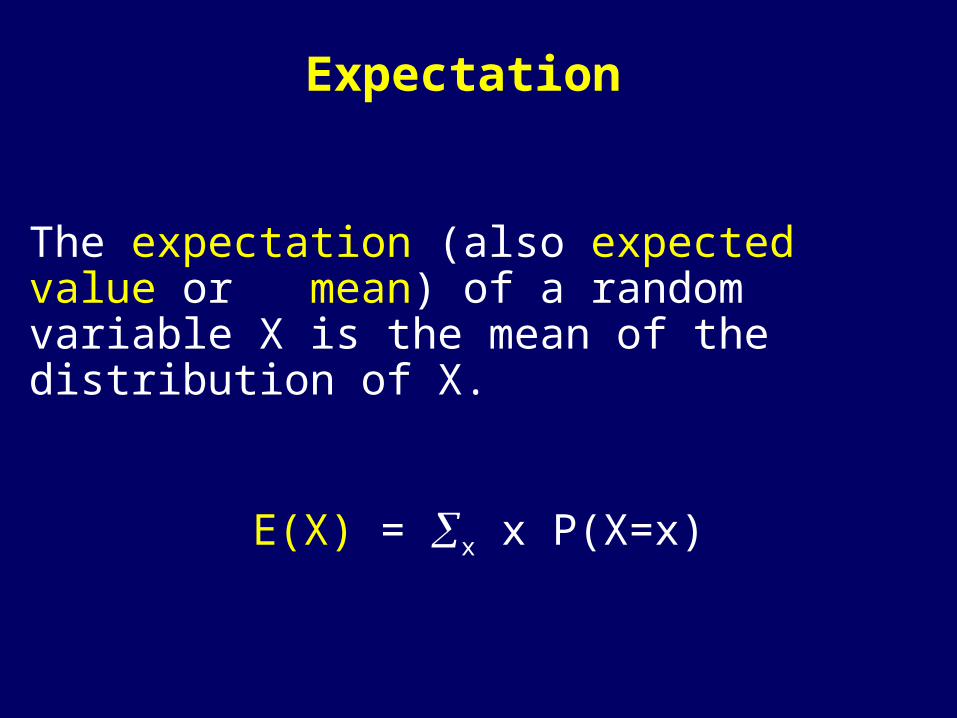
The expectation (also expected value or mean) of a random variable X is the mean of the distribution of X.

E(X) = x x P(X=x)

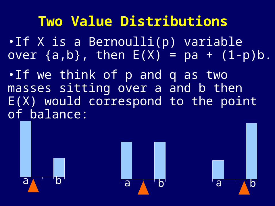
Two Value Distributions•If X is a Bernoulli(p) variable over {a,b}, then E(X) = pa + (1-p)b.

•If we think of p and q as two masses sitting over a and b then E(X) would correspond to the point of balance:

a a ab b b

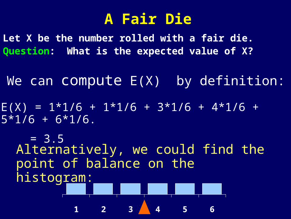
A Fair DieLet X be the number rolled with a fair die. Question: What is the expected value of X?

1 2 3 4 5 6

Alternatively, we could find the point of balance on the histogram:

We can compute E(X) by definition:

E(X) = 1*1/6 + 1*1/6 + 3*1/6 + 4*1/6 + 5*1/6 + 6*1/6.

= 3.5

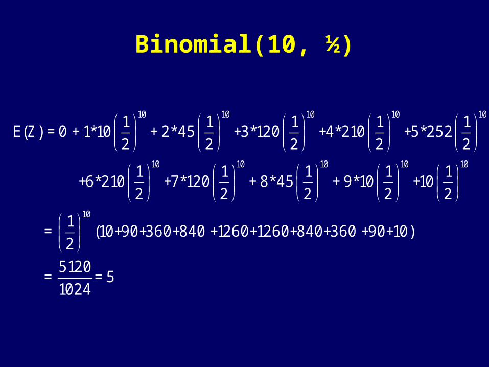
Binomial(10, ½)

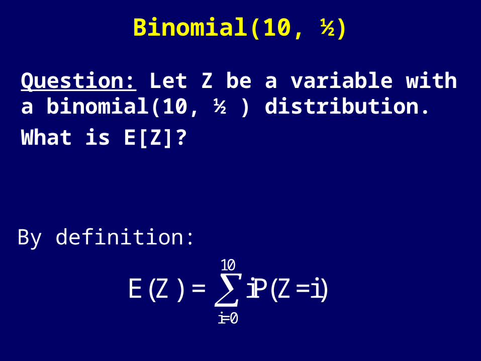
Question: Let Z be a variable with a binomial(10, ½ ) distribution.What is E[Z]?

10

i=0

E(Z) = iP(Z=i) By definition:

Binomial(10, ½)

10 10 10 10 10

10 10 10 10 10

10

1 1 1 1 1E(Z) = 0 + 1*10 + 2*45 +3*120 +4*210 +5*252

2 2 2 2 2

1 1 1 1 1 +6*210 +7*120 + 8*45 + 9*10 +10

2 2 2 2 2

1 =

2

(10+90+360+840 +1260+1260+840+360 +90+10)

5120 = = 5

1024

Binomial(10, ½)

0.

0.1

0.2

0.3

0 1 2 3 4 5 6 7 8 9 10

We could also look at the histogram:

Addition Rule

•For any two random variables X and Y defined over the same sample space

E(X+Y) = E(X) + E(Y).

•Consequently, for a sequence of random variables X1,X2,…,Xn,

E(X1+X2+…+Xn) = E(X1) + E(X2) +…+ E(Xn).

• Therefore the mean of Bin(10,1/2) = 5.

Multiplication Rule and Inequalities

•Multiplication rule: E[aX] = a E[X].

•E[aX] = x a x P[X = x] = a x P[X = x] = a E[x]

•If X ¸ Y then E[X] ¸ E[Y].•This follows since X-Y is non negative and •E[X] – E[Y] = E[X-Y] ¸ 0.

Sum of Two Dice•Let T be the sum of two dice. What’s E(T)?

•The “easy” way: E(T) = t tP(T=t).

This sum will have 11 terms.

•We could also find the center of mass of the histogram (easy to do by symmetry).

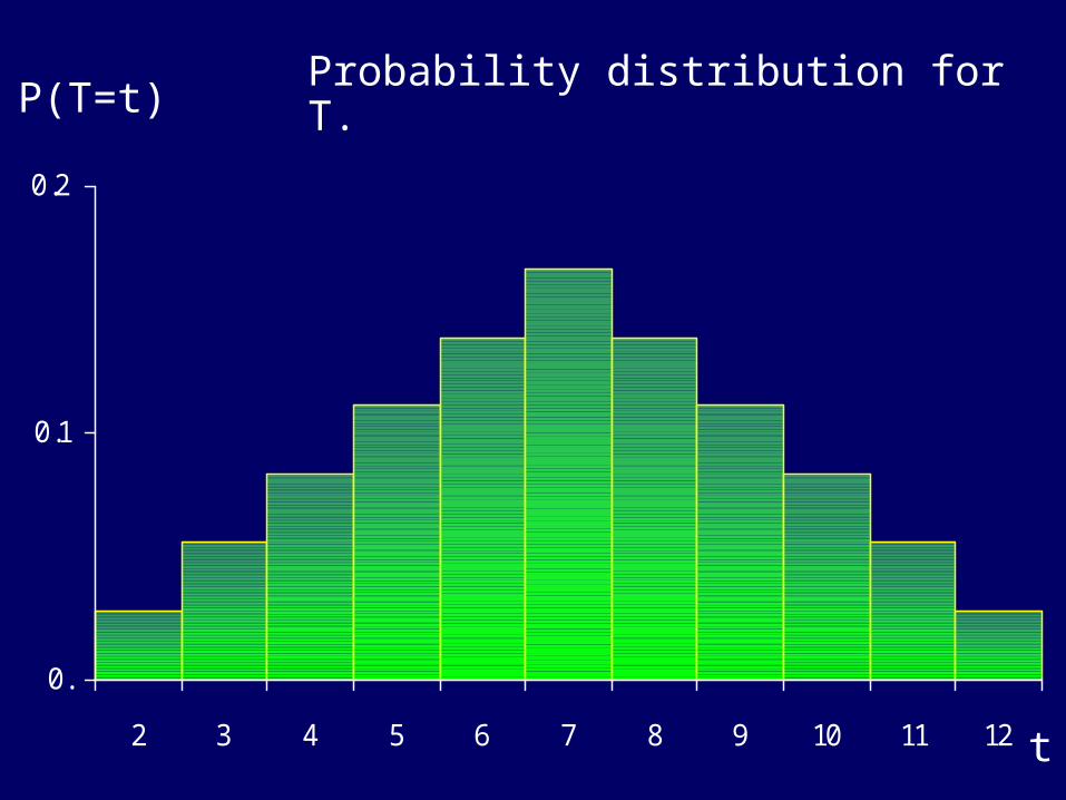
histogram for TProbability distribution for T.

0.

0.1

0.2

2 3 4 5 6 7 8 9 10 11 12 t

P(T=t)

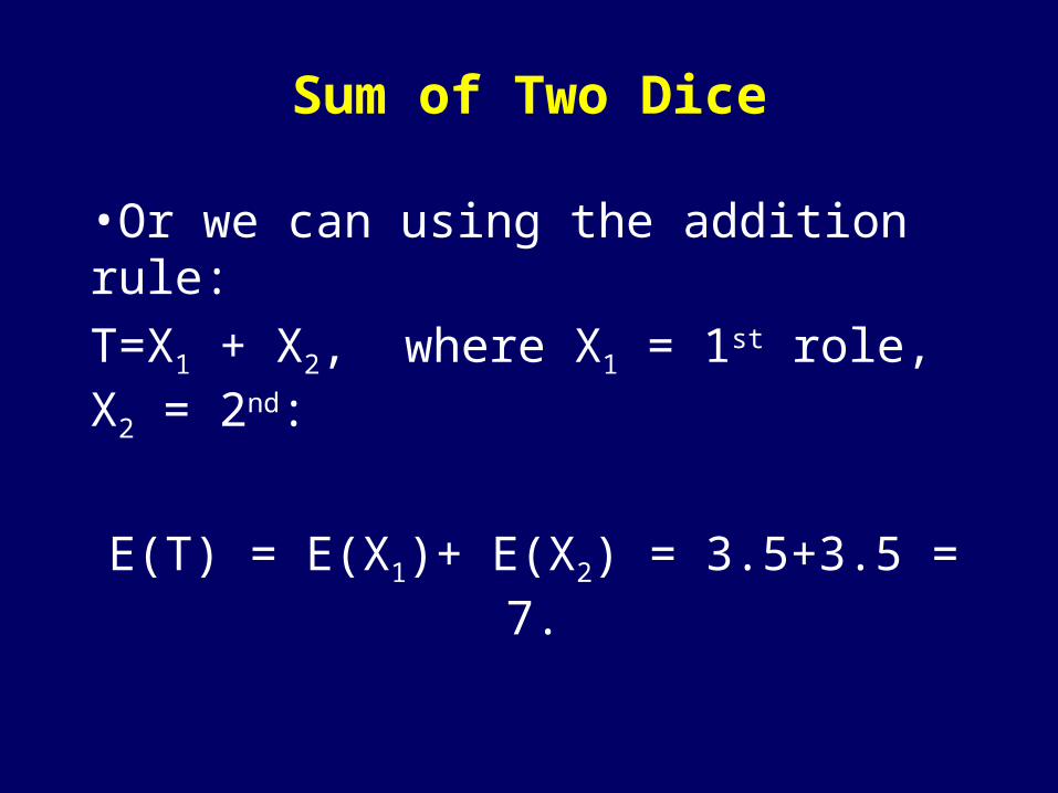
Sum of Two Dice

•Or we can using the addition rule: T=X1 + X2, where X1 = 1st role, X2 = 2nd:

E(T) = E(X1)+ E(X2) = 3.5+3.5 = 7.

Indicators

Indicators associate 0/1 valued random variables to events.

Definition: The indicator of the event A,

IA is the random variable that takes the value 1 for outcomes in A and the value 0 for outcomes in Ac.

Indicators

Suppose IA is an indicator of an event A with probability p.

Ac AIA=1IA=0

Expectation of Indicators

Then:

E(IA)= 1*P(A) + 0*P(Ac) = P(A) = p.

P(Ac) P(A)IA=1IA=0

Expected Number of Events that Occur

•Suppose there are n events A1, A2, …, An.

• Let X = I1 + I2 + … + In where Ii is the indicator of Ai

• Then X counts the number of events that occur.

•By the addition rule:

E(X) = P(A1) + P(A2) + … P(An).

Repeated Trials

•Let Xi = indicator of success on the ith

coin toss (Xi = 1 if the ith coin toss = H head, and Xi = 0 otherwise).•The sequence X1 , X2 , … , Xn is a sequence of n independent variables with Bernoulli(p) distribution over {0,1}.•The number of heads in n coin tosses given by Sn = X1 + X2 + … + Xn.

•E(Sn) = nE(Xi) = np

•Thus the mean of Bin(n,p) RV = np.

Expected Number of Aces

•Let Y be the number of aces in a poker hand.•Then:Y = I1st ace + I3rd ace + I4th ace + I5th ace + I2nd ace .

•And: E(Y) = 5*P(ace) = 5*4/52 = 0.385.•Alternatively, since Y has the hyper-geometric distribution we can calculate:

44

52

5

48

5-y

x=0

yE(Y) = y

Non-negative Integer Valued RV

•Suppose X is an integer valued, non-negative random variable.

•Let Ai = {X ¸ i} for i=1,2,…;

•Let Ii the indicator of the set Ai.

•Then

X=i Ii.

Non-negative Integer Valued RV

•The equality

X(outcome)=i Ii(outcome)

follows since if X(outcome) = i, then

outcome2 A1ÅA2Å…ÅAi. but not to Aj, j>i.

•So (I1+I2+…+I

i+I

i+1+…)(outcome) =

1+1+…+1+0+0+… = i.

Tail Formula for ExpectationLet X be a non-negative integer valued RV,

Then:

E(X) = E (i Ii ) = i E( Ii )

E(X) = i P(X¸ i), i=1,2,3…… …

P(X≥4) P(X=4) …

P(X≥3) P(X=3) P(X=4) …

P(X≥2) P(X=2) P(X=3) P(X=4) …

P(X≥1) P(X=1) P(X=2) P(X=3) P(X=4) …E(X) = 1*P(X=1) 2*P(X=2) 3*P(X=3) 4*P(X=4) …

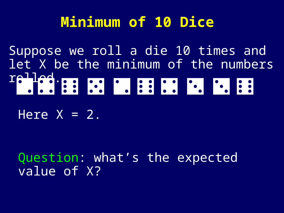
Minimum of 10 Dice

Suppose we roll a die 10 times and let X be the minimum of the numbers rolled.

Here X = 2.

Question: what’s the expected value of X?

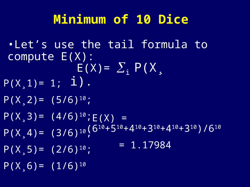
Minimum of 10 Dice

•Let’s use the tail formula to compute E(X):

E(X)= i P(X¸ i). P(X¸1)= 1;

P(X¸2)= (5/6)10;

P(X¸3)= (4/6)10;

P(X¸4)= (3/6)10;

P(X¸5)= (2/6)10;

P(X¸6)= (1/6)10

E(X) = (610+510+410+310+410+310)/610

E(X) = 1.17984

Indicators

•If the events A1, A2, …, Aj are mutually exclusive then

I1 + I2 +… + Ij = IA1 [ A2 [ … [ Aj

•And

P([ji=1 Ai) = i P(Ai).

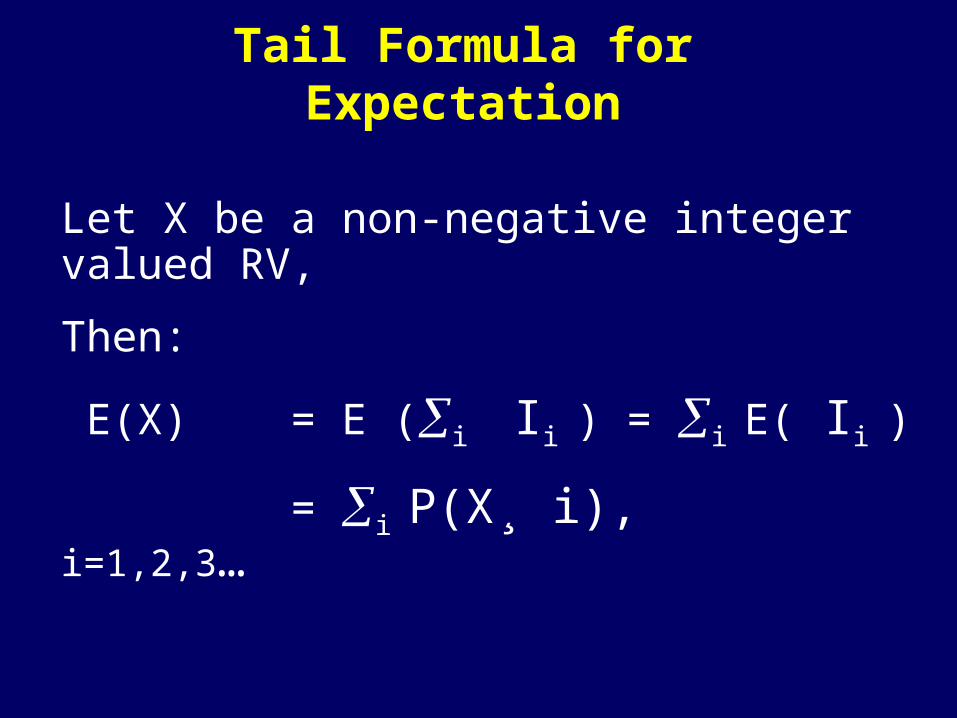
Tail Formula for Expectation

Let X be a non-negative integer valued RV,

Then:

E(X) = E (i Ii ) = i E( Ii )

E(X) = i P(X¸ i), i=1,2,3…

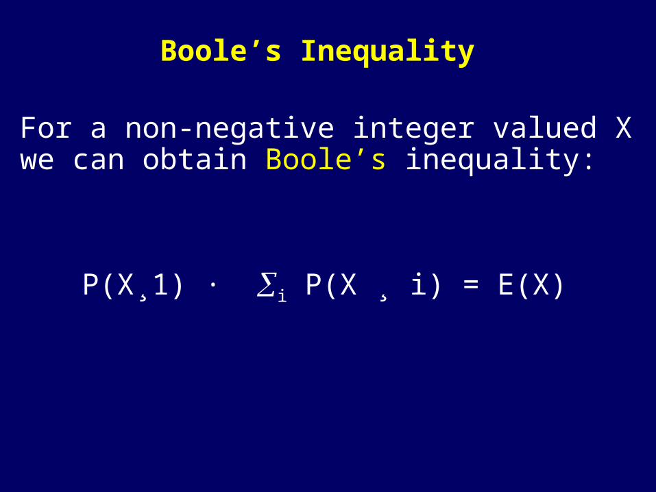
Boole’s Inequality

For a non-negative integer valued X we can obtain Boole’s inequality:

P(X¸1) · i P(X ¸ i) = E(X)

Markov’s InequalityMarkov inequality:If X¸0, then for every a > 0

P(X¸a) · E(X)/a.

•This is proven as follows.• Note that if X ¸ Y then E(X) ¸ E(Y).•Take Y = indicator of the event {X ¸ a}.•Then E(Y) = P(X ¸ a) and X ¸ aY so:• E(X) ¸ E(aY) = a E(Y) = a P(X ¸ a).

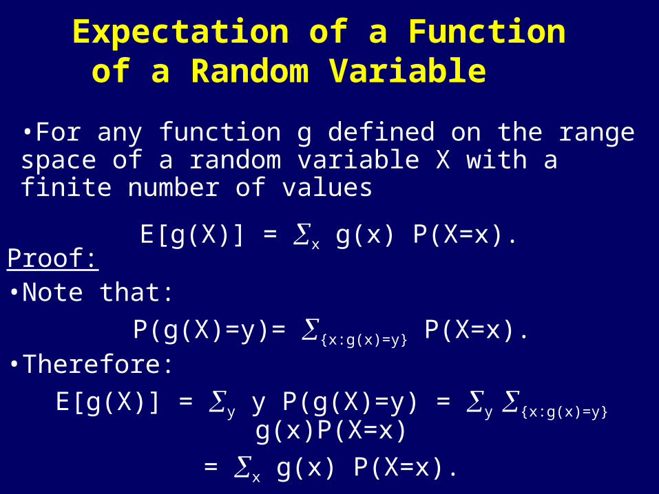
Expectation of a Function of a Random Variable

•For any function g defined on the range space of a random variable X with a finite number of values

E[g(X)] = x g(x) P(X=x).Proof: •Note that:

P(g(X)=y)= {x:g(x)=y} P(X=x).•Therefore:E[g(X)] = y y P(g(X)=y) = y {x:g(x)=y} g(x)P(X=x)

= x g(x) P(X=x).

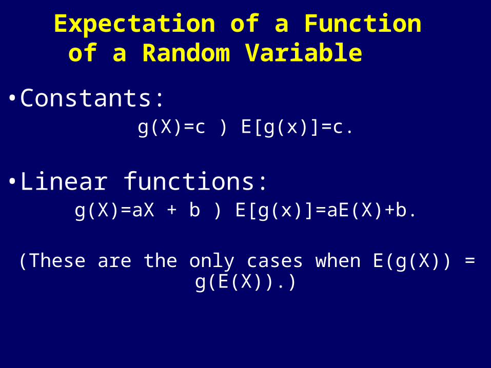
Expectation of a Function of a Random Variable

•Constants: g(X)=c ) E[g(x)]=c.

•Linear functions: g(X)=aX + b ) E[g(x)]=aE(X)+b.

(These are the only cases when E(g(X)) = g(E(X)).)

Expectation of a Function of a Random Variable

•Monomials: g(X)=Xk ) E[g(x)]=x xkP(X=x).

x xkP(X=x) is called the kth moment of X.

Expectation of a Function of a Random Variable

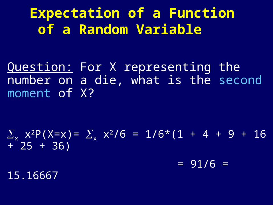
Question: For X representing the number on a die, what is the second moment of X?

x x2P(X=x)= x x2/6 = 1/6*(1 + 4 + 9 + 16 + 25 + 36)

= 91/6 = 15.16667

Expectation of a Function of Several Random Variables

•If X and Y are two random variables we obtain:E(g(X,Y))= {all (x,y)} g(x,y)P(X=x, Y=y).

This allows to prove that E[X+Y] = E[X] + E[Y]:

E(X) = {all (x,y)} x P(X=x, Y=y);

E(Y) = {all (x,y)} y P(X=x, Y=y);

E(X+Y) = {all (x,y)} (x+y) P(X=x, Y=y);

E(X+Y) = E(X) + E (Y)

Expectation of a Function of Several Random Variables

E(g(X,Y))= {all (x,y)} g(x,y)P(X=x, Y=y).

Product:E(XY) = {all (x,y)} xy P(X=x, Y=y);

E(XY) = x y xy P(X=x, Y=y);

Is E(XY) = E(X)E(Y)?

Product Rule for Independent Random

Variables•However, if X and Y are independent,

P(X=x,Y=y)=P(X=x)P(Y=y)then product formula simplifies:

E(XY) = x y xy P(X=x) P(Y=y)

= (xx P(X=x)) (y y P(Y=y)) =

E(X) E(Y) •If X and Y are independent then:

E(XY) =E(X) E(Y);

Expectation interpretation as a Long-Run Average

•If we repeatedly sample from the distribution of X then P(X=x) will be close to the observed frequency of x in the sample.

•E(X) will be approximately the long-run average of the sample.

Mean, Mode and Median• The Mode of X is the most likely possible value of X. • The mode need not be unique.

• The Median of X is a number m such that both P(X·m) ¸ ½ and P(X ¸ m) ¸ ½. • The median may also not be unique.

•Mean and Median are not necessarily possible values (mode is).

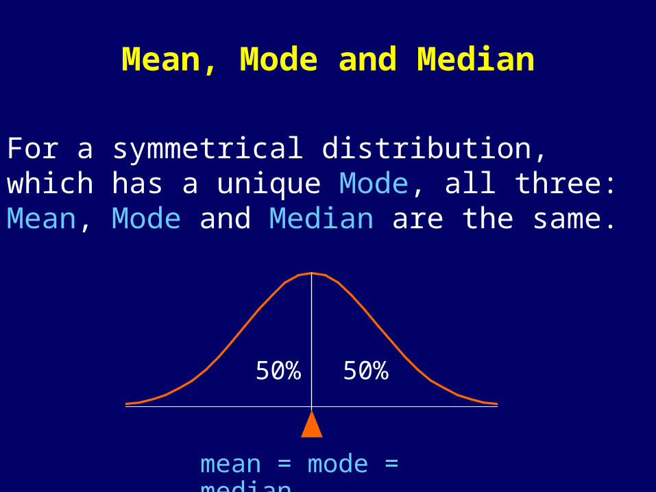
Mean, Mode and Median

For a symmetrical distribution, which has a unique Mode, all three: Mean, Mode and Median are the same.

mean = mode = median

50%

50%

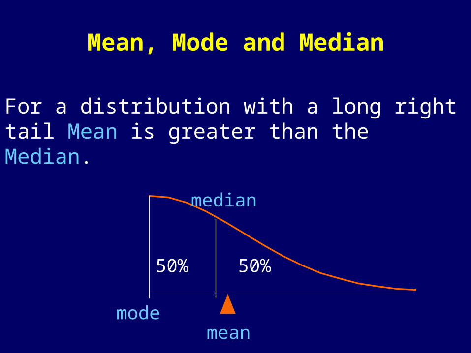
Mean, Mode and Median

For a distribution with a long right tail Mean is greater than the Median.

mean

50%

50%

mode

median

Roulette

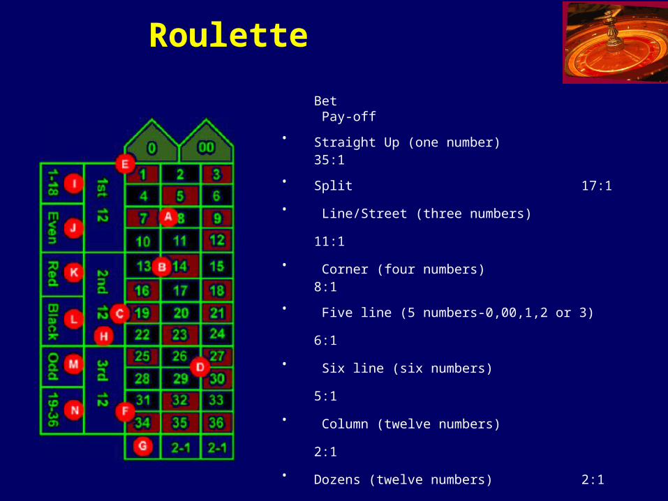
Bet Pay-off

• Straight Up (one number) 35:1

• Split 17:1 • Line/Street (three numbers) 11:1 • Corner (four numbers)

8:1

• Five line (5 numbers-0,00,1,2 or 3) 6:1 • Six line (six numbers)

5:1 • Column (twelve numbers) 2:1 • Dozens (twelve numbers) 2:1 • 1 - 18 1:1 • Even 1:1 • Red

1:1

• Black 1:1 • Odd 1:1 • 19-36 1:1

Betting on Red

Suppose we want to be $1 on Red. Our chance of winning is 18/38.

Question:What should be the pay-off to make it a fair bet?

Betting on Red

This question really only makes sense if we repeatedly bet $1 on Red.

Suppose that we could win $x if Reds come up and lose $1, otherwise. If X denotes our returns then P(X=x) = 18/38; P(X=-1)=20/38.

In a fair game, we expect to break even on average.

Betting on Red

Our expected return is:x*18/38 - 1*20/38.

Setting this to zero gives us x=20/18=1.1111111… .

This is greater than the pay-off of 1:1 that is offered by the casino.