lecture18 - people | mit csail
TRANSCRIPT

Naïve Bayes & Logis/c Regression Lecture 18
David Sontag New York University
Slides adapted from Vibhav Gogate, Luke Zettlemoyer, Carlos Guestrin, and Dan Weld

Naïve Bayes • Naïve Bayes assump:on:
– Features are independent given class:
– More generally:
• How many parameters now? • Suppose X is composed of n binary features

The Naïve Bayes Classifier • Given:
– Prior P(Y) – n condi:onally independent features X given the class Y
– For each Xi, we have likelihood P(Xi|Y)
• Decision rule:
If certain assumption holds, NB is optimal classifier! (they typically don’t)
Y
X1 Xn X2
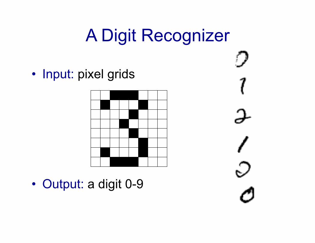
A Digit Recognizer
• Input: pixel grids
• Output: a digit 0-9

Naïve Bayes for Digits (Binary Inputs)
• Simple version: – One feature Fij for each grid position <i,j>
– Possible feature values are on / off, based on whether intensity is more or less than 0.5 in underlying image
– Each input maps to a feature vector, e.g.
– Here: lots of features, each is binary valued
• Naïve Bayes model:
• Are the features independent given class?
• What do we need to learn?

Example Distributions
1 0.1
2 0.1
3 0.1
4 0.1
5 0.1
6 0.1
7 0.1
8 0.1
9 0.1
0 0.1
1 0.01
2 0.05
3 0.05
4 0.30
5 0.80
6 0.90
7 0.05
8 0.60
9 0.50
0 0.80
1 0.05
2 0.01
3 0.90
4 0.80
5 0.90
6 0.90
7 0.25
8 0.85
9 0.60
0 0.80

MLE for the parameters of NB • Given dataset
– Count(A=a,B=b) Ã number of examples where A=a and B=b
• MLE for discrete NB, simply: – Prior:
– Likelihood:
µMLE ,σMLE = argmaxµ,σ
P (D | µ,σ)
= −N�
i=1
(xi − µ)
σ2= 0
= −N�
i=1
xi +Nµ = 0
= −N
σ+
N�
i=1
(xi − µ)2
σ3= 0
argmaxwln
�1
σ√2π
�N
+N�
j=1
−[tj −�
iwihi(xj)]2
2σ2
= argmaxw
N�
j=1
−[tj −�
iwihi(xj)]2
2σ2
= argminw
N�
j=1
[tj −�
i
wihi(xj)]2
P (Y = y) =Count(Y = y)�y� Count(Y = y�)
2
µMLE ,σMLE = argmaxµ,σ
P (D | µ,σ)
= −N�
i=1
(xi − µ)
σ2= 0
= −N�
i=1
xi +Nµ = 0
= −N
σ+
N�
i=1
(xi − µ)2
σ3= 0
argmaxwln
�1
σ√2π
�N
+N�
j=1
−[tj −�
iwihi(xj)]2
2σ2
= argmaxw
N�
j=1
−[tj −�
iwihi(xj)]2
2σ2
= argminw
N�
j=1
[tj −�
i
wihi(xj)]2
P (Y = y) =Count(Y = y)�y� Count(Y = y�)
2
µMLE ,σMLE = argmaxµ,σ
P (D | µ,σ)
= −N�
i=1
(xi − µ)
σ2= 0
= −N�
i=1
xi +Nµ = 0
= −N
σ+
N�
i=1
(xi − µ)2
σ3= 0
argmaxwln
�1
σ√2π
�N
+N�
j=1
−[tj −�
iwihi(xj)]2
2σ2
= argmaxw
N�
j=1
−[tj −�
iwihi(xj)]2
2σ2
= argminw
N�
j=1
[tj −�
i
wihi(xj)]2
P (Y = y) =Count(Y = y)�y� Count(Y = y�)
P (Xi = x|Y = y) =Count(Xi = x, Y = y)�x� Count(Xi = x�, Y = y)
2

Subtle:es of NB classifier – Viola:ng the NB assump:on
• Usually, features are not condi:onally independent:
• Actual probabili:es P(Y|X) oVen biased towards 0 or 1 (i.e., not well “calibrated”)
• Nonetheless, NB oVen performs well, even when assump:on is violated
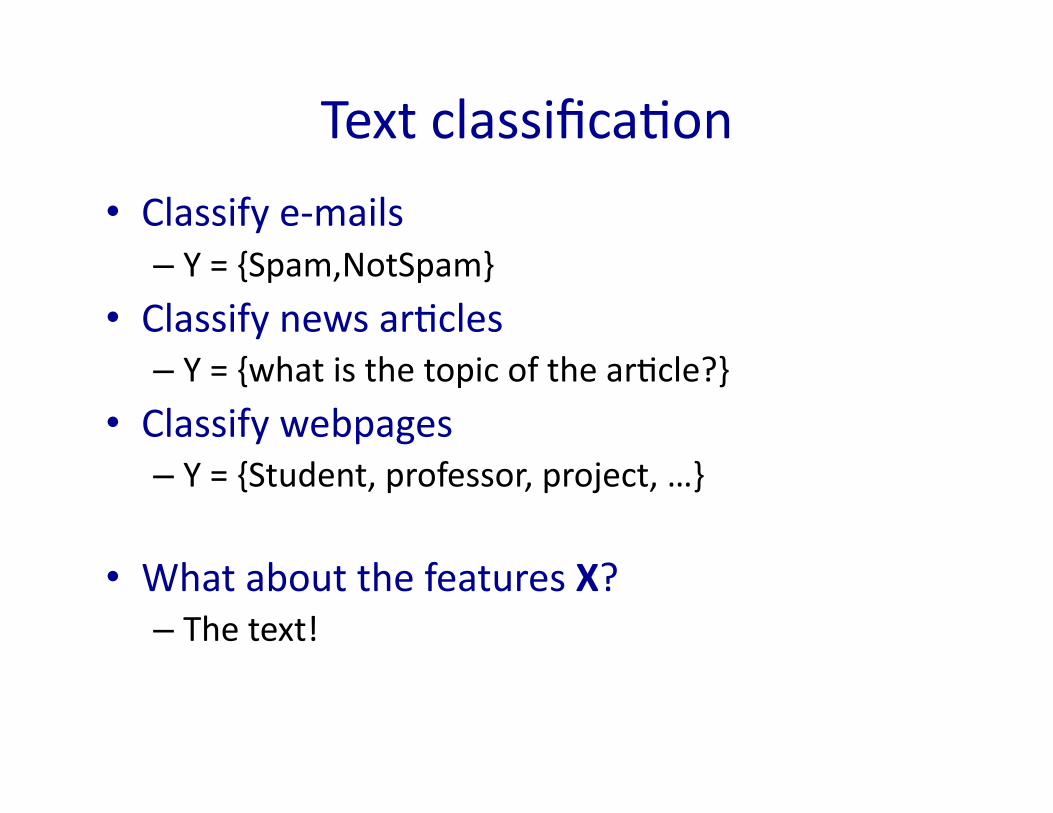
Text classifica:on
• Classify e-‐mails – Y = {Spam,NotSpam}
• Classify news ar:cles – Y = {what is the topic of the ar:cle?}
• Classify webpages – Y = {Student, professor, project, …}
• What about the features X? – The text!

Features X are en:re document – Xi for ith word in ar:cle
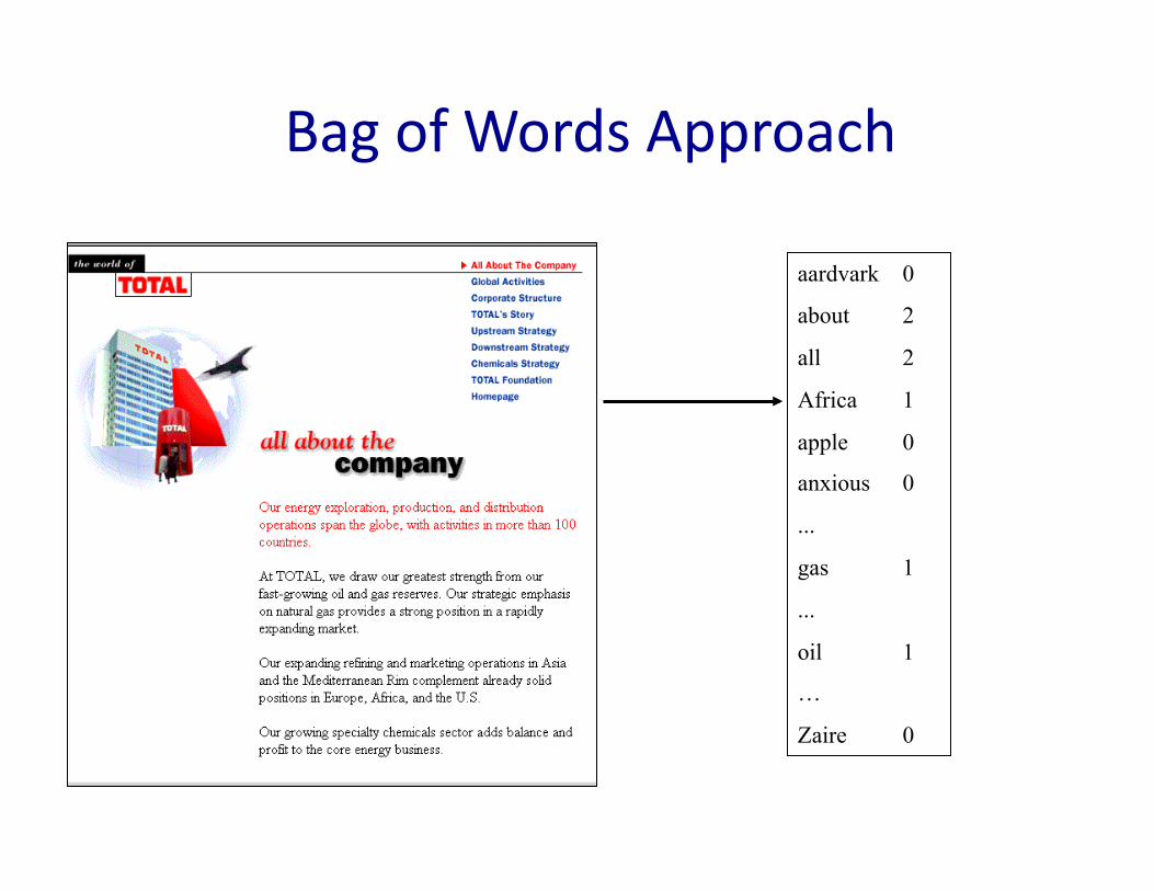
Bag of Words Approach
aardvark 0
about 2
all 2
Africa 1
apple 0
anxious 0
...
gas 1
...
oil 1
…
Zaire 0

NB with Bag of Words for text classifica:on
• Learning phase: – Prior P(Y)
• Count number of documents for each topic
– P(Xi|Y) • Just considering the documents assigned to topic Y, find the frac:on of docs containing a given word; remember this dist’n is shared across all posi:ons i
• Test phase: – For each document
• Use naïve Bayes decision rule

pageMehryar Mohri - Introduction to Machine Learning
Naive Bayes = Linear Classifier
Theorem: assume that for all . Then, the Naive Bayes classifier is defined by
Proof: observe that for any ,
20
xi ∈ {0, 1} i ∈ [1, N ]
x �→ sgn(w · x + b),
where
and
i ∈ [1, N ]
logPr[xi | +1]Pr[xi | −1]
=�
logPr[xi = 1 | +1]Pr[xi = 1 | −1]
− logPr[xi = 0 | +1]Pr[xi = 0 | −1]
�xi+log
Pr[xi = 0 | +1]Pr[xi = 0 | −1]
.
wi = log Pr[xi=1|+1]Pr[xi=1|−1] − log Pr[xi=0|+1]
Pr[xi=0|−1]
b = log Pr[+1]Pr[−1] +
�Ni=1 log Pr[xi=0|+1]
Pr[xi=0|−1] .
[Slide from Mehyrar Mohri]
pageMehryar Mohri - Introduction to Machine Learning
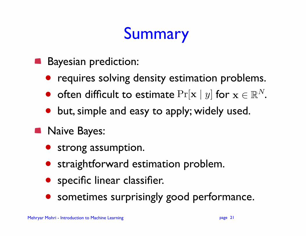
Summary
Bayesian prediction:
• requires solving density estimation problems.
• often difficult to estimate for .
• but, simple and easy to apply; widely used.
Naive Bayes:
• strong assumption.
• straightforward estimation problem.
• specific linear classifier.
• sometimes surprisingly good performance.
21
Pr[x | y] x ∈ RN

Lets take a(nother) probabilis:c approach!!!
• Previously: directly es:mate the data distribu:on P(X,Y)! – challenging due to size of distribu:on!
– make Naïve Bayes assump:on: only need P(Xi|Y)!
• But wait, we classify according to: – maxY P(Y|X)
• Why not learn P(Y|X) directly?

Genera:ve vs. Discrimina:ve Classifiers
• Want to Learn: X Y – X – features – Y – target classes
• Genera/ve classifier, e.g., Naïve Bayes: – Assume some func/onal form for P(X|Y), P(Y) – Es:mate parameters of P(X|Y), P(Y) directly from training data – Use Bayes’ rule to calculate P(Y|X= x) – This is an example of a “genera&ve” model
• Indirect computa:on of P(Y|X) through Bayes rule • As a result, can also generate a sample of the data, P(X) = ∑y P(y) P(X|y)
– Can easily handle missing data
• Discrimina/ve classifiers, e.g., Logis:c Regression: – Assume some func/onal form for P(Y|X) – Es:mate parameters of P(Y|X) directly from training data – This is the “discrimina&ve” (or “condi/onal”) model
• Directly learn P(Y|X) • But cannot obtain a sample of the data, because P(X) is not available
P(Y | X) ∝ P(X | Y) P(Y)
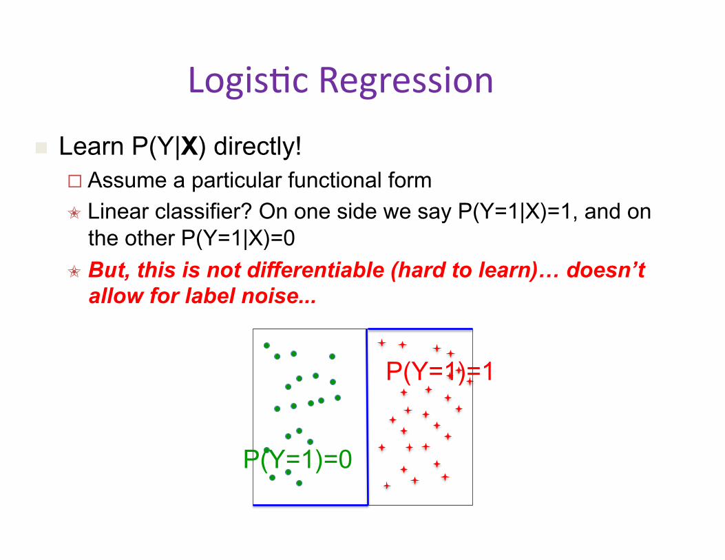
Logis:c Regression
Learn P(Y|X) directly! Assume a particular functional form
✬ Linear classifier? On one side we say P(Y=1|X)=1, and on the other P(Y=1|X)=0
✬ But, this is not differentiable (hard to learn)… doesn’t allow for label noise...
P(Y=1)=0
P(Y=1)=1

Logis:c Regression Logistic function (Sigmoid):
• Learn P(Y|X) directly! • Assume a particular
functional form
• Sigmoid applied to a linear function of the data:
Features can be discrete or continuous!
Copyright c� 2010, Tom M. Mitchell. 7
where the superscript j refers to the jth training example, and where δ(Y = yk) is
1 if Y = yk and 0 otherwise. Note the role of δ here is to select only those training
examples for which Y = yk.
The maximum likelihood estimator for σ2
ik is
σ̂2
ik =1
∑ j δ(Y j = yk) ∑j(X j
i − µ̂ik)2δ(Y j = yk) (14)
This maximum likelihood estimator is biased, so the minimum variance unbi-
ased estimator (MVUE) is sometimes used instead. It is
σ̂2
ik =1
(∑ j δ(Y j = yk))−1∑
j(X j
i − µ̂ik)2δ(Y j = yk) (15)
3 Logistic RegressionLogistic Regression is an approach to learning functions of the form f : X →Y , or
P(Y |X) in the case where Y is discrete-valued, and X = �X1 . . .Xn� is any vector
containing discrete or continuous variables. In this section we will primarily con-
sider the case where Y is a boolean variable, in order to simplify notation. In the
final subsection we extend our treatment to the case where Y takes on any finite
number of discrete values.
Logistic Regression assumes a parametric form for the distribution P(Y |X),then directly estimates its parameters from the training data. The parametric
model assumed by Logistic Regression in the case where Y is boolean is:
P(Y = 1|X) =1
1+ exp(w0 +∑ni=1
wiXi)(16)
and
P(Y = 0|X) =exp(w0 +∑n
i=1wiXi)
1+ exp(w0 +∑ni=1
wiXi)(17)
Notice that equation (17) follows directly from equation (16), because the sum of
these two probabilities must equal 1.
One highly convenient property of this form for P(Y |X) is that it leads to a
simple linear expression for classification. To classify any given X we generally
want to assign the value yk that maximizes P(Y = yk|X). Put another way, we
assign the label Y = 0 if the following condition holds:
1 <P(Y = 0|X)P(Y = 1|X)
substituting from equations (16) and (17), this becomes
1 < exp(w0 +n
∑i=1
wiXi)
z
1
1 + e−z

Logis:c Func:on in n Dimensions
-2 0 2 4 6-4-2 0 2 4 6 8 10 0 0.2 0.4 0.6 0.8 1x1x2
Sigmoid applied to a linear function of the data:
Features can be discrete or continuous!
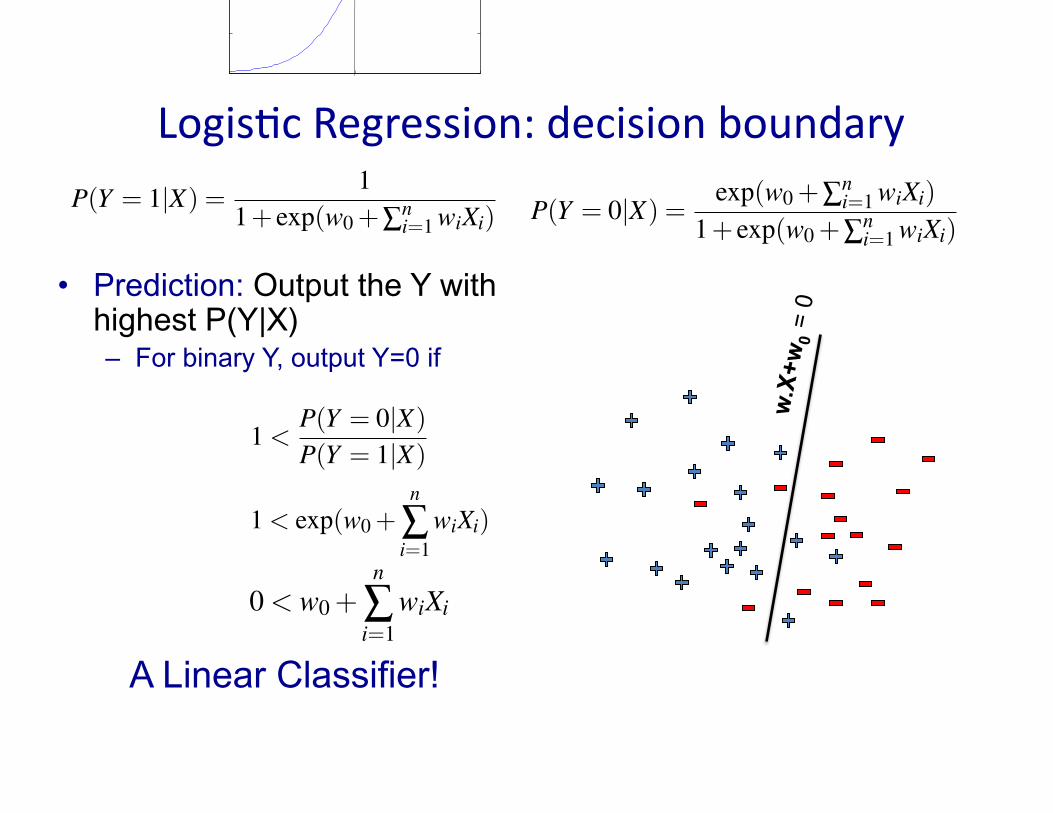
Logis:c Regression: decision boundary
A Linear Classifier!
• Prediction: Output the Y with highest P(Y|X) – For binary Y, output Y=0 if
Copyright c� 2010, Tom M. Mitchell. 7
where the superscript j refers to the jth training example, and where δ(Y = yk) is
1 if Y = yk and 0 otherwise. Note the role of δ here is to select only those training
examples for which Y = yk.
The maximum likelihood estimator for σ2
ik is
σ̂2
ik =1
∑ j δ(Y j = yk) ∑j(X j
i − µ̂ik)2δ(Y j = yk) (14)
This maximum likelihood estimator is biased, so the minimum variance unbi-
ased estimator (MVUE) is sometimes used instead. It is
σ̂2
ik =1
(∑ j δ(Y j = yk))−1∑
j(X j
i − µ̂ik)2δ(Y j = yk) (15)
3 Logistic RegressionLogistic Regression is an approach to learning functions of the form f : X →Y , or
P(Y |X) in the case where Y is discrete-valued, and X = �X1 . . .Xn� is any vector
containing discrete or continuous variables. In this section we will primarily con-
sider the case where Y is a boolean variable, in order to simplify notation. In the
final subsection we extend our treatment to the case where Y takes on any finite
number of discrete values.
Logistic Regression assumes a parametric form for the distribution P(Y |X),then directly estimates its parameters from the training data. The parametric
model assumed by Logistic Regression in the case where Y is boolean is:
P(Y = 1|X) =1
1+ exp(w0 +∑ni=1
wiXi)(16)
and
P(Y = 0|X) =exp(w0 +∑n
i=1wiXi)
1+ exp(w0 +∑ni=1
wiXi)(17)
Notice that equation (17) follows directly from equation (16), because the sum of
these two probabilities must equal 1.
One highly convenient property of this form for P(Y |X) is that it leads to a
simple linear expression for classification. To classify any given X we generally
want to assign the value yk that maximizes P(Y = yk|X). Put another way, we
assign the label Y = 0 if the following condition holds:
1 <P(Y = 0|X)P(Y = 1|X)
substituting from equations (16) and (17), this becomes
1 < exp(w0 +n
∑i=1
wiXi)
Copyright c� 2010, Tom M. Mitchell. 8
−5 0 50
0.2
0.4
0.6
0.8
1
Y
X
Y = 1/(1 + exp(−X))
Figure 1: Form of the logistic function. In Logistic Regression, P(Y |X) is as-
sumed to follow this form.
and taking the natural log of both sides we have a linear classification rule that
assigns label Y = 0 if X satisfies
0 < w0 +n
∑i=1
wiXi (18)
and assigns Y = 1 otherwise.
Interestingly, the parametric form of P(Y |X) used by Logistic Regression is
precisely the form implied by the assumptions of a Gaussian Naive Bayes classi-
fier. Therefore, we can view Logistic Regression as a closely related alternative to
GNB, though the two can produce different results in many cases.
3.1 Form of P(Y |X) for Gaussian Naive Bayes ClassifierHere we derive the form of P(Y |X) entailed by the assumptions of a Gaussian
Naive Bayes (GNB) classifier, showing that it is precisely the form used by Logis-
tic Regression and summarized in equations (16) and (17). In particular, consider
a GNB based on the following modeling assumptions:
• Y is boolean, governed by a Bernoulli distribution, with parameter π =P(Y = 1)
• X = �X1 . . .Xn�, where each Xi is a continuous random variable
w.X
+w
0 =
0
Copyright c� 2010, Tom M. Mitchell. 7
where the superscript j refers to the jth training example, and where δ(Y = yk) is
1 if Y = yk and 0 otherwise. Note the role of δ here is to select only those training
examples for which Y = yk.
The maximum likelihood estimator for σ2
ik is
σ̂2
ik =1
∑ j δ(Y j = yk) ∑j(X j
i − µ̂ik)2δ(Y j = yk) (14)
This maximum likelihood estimator is biased, so the minimum variance unbi-
ased estimator (MVUE) is sometimes used instead. It is
σ̂2
ik =1
(∑ j δ(Y j = yk))−1∑
j(X j
i − µ̂ik)2δ(Y j = yk) (15)
3 Logistic RegressionLogistic Regression is an approach to learning functions of the form f : X →Y , or
P(Y |X) in the case where Y is discrete-valued, and X = �X1 . . .Xn� is any vector
containing discrete or continuous variables. In this section we will primarily con-
sider the case where Y is a boolean variable, in order to simplify notation. In the
final subsection we extend our treatment to the case where Y takes on any finite
number of discrete values.
Logistic Regression assumes a parametric form for the distribution P(Y |X),then directly estimates its parameters from the training data. The parametric
model assumed by Logistic Regression in the case where Y is boolean is:
P(Y = 1|X) =1
1+ exp(w0 +∑ni=1
wiXi)(16)
and
P(Y = 0|X) =exp(w0 +∑n
i=1wiXi)
1+ exp(w0 +∑ni=1
wiXi)(17)
Notice that equation (17) follows directly from equation (16), because the sum of
these two probabilities must equal 1.
One highly convenient property of this form for P(Y |X) is that it leads to a
simple linear expression for classification. To classify any given X we generally
want to assign the value yk that maximizes P(Y = yk|X). Put another way, we
assign the label Y = 0 if the following condition holds:
1 <P(Y = 0|X)P(Y = 1|X)
substituting from equations (16) and (17), this becomes
1 < exp(w0 +n
∑i=1
wiXi)

Understanding Sigmoids
w0=0, w1=-1
w0=-2, w1=-1
w0=0, w1= -0.5
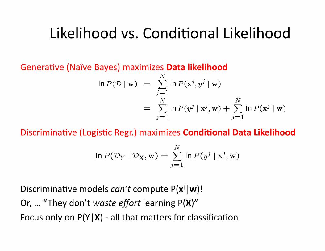
Genera:ve (Naïve Bayes) maximizes Data likelihood
Discrimina:ve (Logis:c Regr.) maximizes Condi/onal Data Likelihood
Discrimina:ve models can’t compute P(xj|w)! Or, … “They don’t waste effort learning P(X)”
Focus only on P(Y|X) -‐ all that maiers for classifica:on
Likelihood vs. Condi:onal Likelihood