Unsupervised  learning  Lecture  13  

David  Sontag  New  York  University  

Slides  adapted  from  Carlos  Guestrin,  Dan  Klein,  Luke  Ze@lemoyer,  Dan  Weld,  Vibhav  Gogate,  and  Andrew  Moore  

Gaussian  Mixture  Models  

µ1 µ2

µ3

•  P(Y):  There  are  k  components  

•  P(X|Y):  Each  component  generates  data  from  a  mul5variate  Gaussian  with  mean  μi  and  covariance  matrix  Σi  

Each  data  point  is  sampled  from  a  genera&ve  process:    

1.  Choose  component  i  with  probability  P(y=i)          [Mul-nomial]  

2.  Generate  datapoint  ~  N(mi,  Σi  )  

€

P(X = x j |Y = i) =

1(2π)m / 2 ||Σi ||

1/ 2 exp −12x j − µi( )

TΣi−1 x j − µi( )⎡

⎣ ⎢ ⎤

⎦ ⎥

ML  esVmaVon  in  supervised  seWng  

•  Univariate  Gaussian  

•  Mixture  of  Mul&variate  Gaussians  

ML  esVmate  for  each  of  the  MulVvariate  Gaussians  is  given  by:  

Just  sums  over  x  generated  from  the  k’th  Gaussian  

µML =1n

xnj=1

n

∑ ΣML =1n

x j −µML( ) x j −µML( )T

j=1

n

∑k   k   k   k  

What  about  with  unobserved  data?  

•  Maximize  marginal  likelihood:  – argmaxθ  ∏j  P(xj)  =  argmax  ∏j  ∑k=1  P(Yj=k,  xj)  

•  Almost  always  a  hard  problem!  – Usually  no  closed  form  soluVon  

– Even  when  lgP(X,Y)  is  convex,  lgP(X)  generally  isn’t…  

– For  all  but  the  simplest  P(X),  we  will  have  to  do  gradient  ascent,  in  a  big  messy  space  with  lots  of  local  opVmum…  

K  

ExpectaVon  MaximizaVon  

1977:  Dempster,  Laird,  &  Rubin  

The  EM  Algorithm  

•  A  clever  method  for  maximizing  marginal  likelihood:  –  argmaxθ  ∏j  P(xj)  =  argmaxθ  ∏j  ∑k=1

K  P(Yj=k,  xj)  

– Based  on  coordinate  descent.  Easy  to  implement  (eg,  no  line  search,  learning  rates,  etc.)  

•  Alternate  between  two  steps:  – Compute  an  expectaVon  – Compute  a  maximizaVon  

•  Not  magic:  s&ll  op&mizing  a  non-­‐convex  func&on  with  lots  of  local  op&ma  –  The  computaVons  are  just  easier  (ofen,  significantly  so!)  

EM:  Two  Easy  Steps  Objec5ve:  argmaxθ  lg∏j  ∑k=1

K  P(Yj=k,  xj  ;  θ)  =  ∑j  lg  ∑k=1K  P(Yj=k,  xj;  θ)    

Data:  {xj  |  j=1  ..  n}    

•  E-­‐step:  Compute  expectaVons  to  “fill  in”  missing  y  values  according  to  current  parameters,  θ    

–  For  all  examples  j  and  values  k  for  Yj,  compute:  P(Yj=k  |  xj;  θ)    

•  M-­‐step:  Re-­‐esVmate  the  parameters  with  “weighted”  MLE  esVmates  

–  Set  θnew  =  argmaxθ  ∑j  ∑k  P(Yj=k  |  xj  ;θold)  log  P(Yj=k,  xj  ;  θ)  

Par5cularly  useful  when  the  E  and  M  steps  have  closed  form  solu5ons  

Gaussian  Mixture  Example:  Start  

Afer  first  iteraVon  

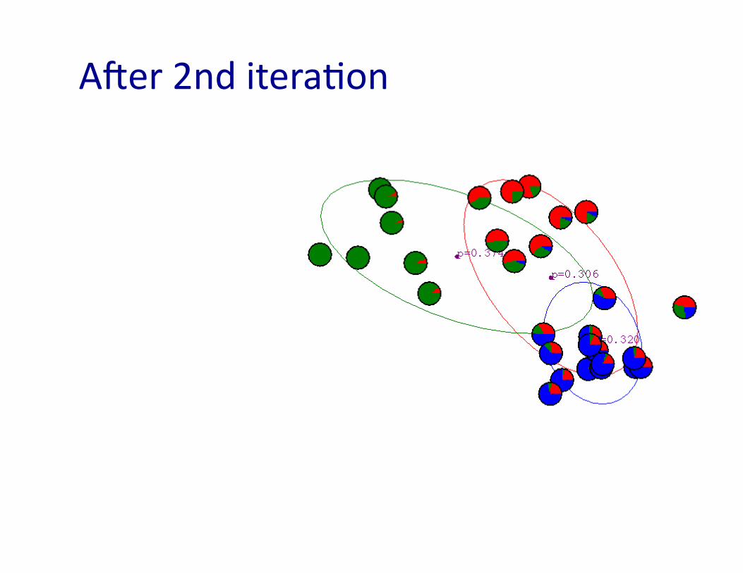
Afer  2nd  iteraVon  

Afer  3rd  iteraVon  

Afer  4th  iteraVon  

Afer  5th  iteraVon  

Afer  6th  iteraVon  

Afer  20th  iteraVon  

Simple  example:  learn  means  only!  Consider:  •  1D  data  •  Mixture  of  k=2  Gaussians  

•  Variances  fixed  to  σ=1  •  DistribuVon  over  classes  is  uniform  

•  Just  need  to  esVmate  μ1  and  μ2  

€

P(x,Yj = k)k=1

K

∑j=1

m

∏ ∝ exp −12σ2

x − µk2⎡

⎣ ⎢ ⎤

⎦ ⎥ P(Yj = k)

k=1

K

∑j=1

m

∏

.01 .03 .05 .07 .09

=2  

EM  for  GMMs:  only  learning  means  Iterate:    On  the  t’th  iteraVon  let  our  esVmates  be  

λt  =  {  μ1(t),  μ2(t)  …  μK(t)  }  E-­‐step  

 Compute  “expected”  classes  of  all  datapoints  

M-­‐step  

 Compute  most  likely  new  μs  given  class  expectaVons  €

P Yj = k x j ,µ1...µK( )∝ exp − 12σ 2 x j − µk

2⎛

⎝ ⎜

⎞

⎠ ⎟ P Yj = k( )

€

µk = P Yj = k x j( )

j=1

m

∑ x j

P Yj = k x j( )j=1

m

∑

E.M.  for  General  GMMs  Iterate:    On  the  t’th  iteraVon  let  our  esVmates  be  

λt  =  {  μ1(t),  μ2(t)  …  μK(t),  Σ1(t),  Σ2

(t)  …  ΣK(t),  p1(t),  p2(t)  …  pK(t)  }  

E-­‐step    Compute  “expected”  classes  of  all  datapoints  for  each  class  

€

P Yj = k x j;λt( )∝ pk( t )p x j ;µk

( t ),Σk(t )( )

pk(t)  is  shorthand  for  esVmate  of  P(y=k)  on  t’th  iteraVon  

M-­‐step      

   Compute  weighted  MLE  for  μ  given  expected  classes  above  

€

µkt+1( ) =

P Yj = k x j;λt( )j∑ x j

P Yj = k x j;λt( )j∑

€

Σkt+1( ) =

P Yj = k x j;λt( )j∑ x j − µk

t+1( )[ ] x j − µkt+1( )[ ]

T

P Yj = k x j ;λt( )j∑

€

pk(t+1) =

P Yj = k x j;λt( )j∑

m m  =  #training  examples  

Just  evaluate  a  Gaussian  at  xj  

What  if  we  do  hard  assignments?  Iterate:    On  the  t’th  iteraVon  let  our  esVmates  be  

λt  =  {  μ1(t),  μ2(t)  …  μK(t)  }  E-­‐step  

 Compute  “expected”  classes  of  all  datapoints  

M-­‐step  

 Compute  most  likely  new  μs  given  class  expectaVons  

€

µk = j=1

m∑ δ Yj = k,x j( ) x j

δ Yj = k,x j( )j=1

m

∑

δ  represents  hard  assignment  to  “most  likely”  or  nearest  cluster  

 Equivalent  to  k-­‐means  clustering  algorithm!!!  

€

P Yj = k x j;µ1...µK( )∝ exp − 12σ 2 x j − µk

2⎛

⎝ ⎜

⎞

⎠ ⎟ P Yj = k( )

€

µk = P Yj = k x j( )

j=1

m

∑ x j

P Yj = k x j( )j=1

m

∑

ProperVes  of  EM  

•  We  will  prove  that  – EM  converges  to  a  local  maxima  

– Each  iteraVon  improves  the  log-­‐likelihood  

•  How?  (Same  as  k-­‐means)  – E-­‐step  can  never  decrease  likelihood  – M-­‐step  can  never  decrease  likelihood  

The  general  learning  problem  with  missing  data  •  Marginal  likelihood:  X  is  observed,  

                             Z  (e.g.  the  class  labels  Y)  is  missing:  

•  ObjecVve:  Find  argmaxθ  l(θ:Data)  •  Assuming  hidden  variables  are  missing  completely  at  random  

(otherwise,  we  should  explicitly  model  why  the  values  are  missing)