lecture notes - university of...
TRANSCRIPT

University of Regina
Statistics 441 – Stochastic Calculus with Applications to Finance
Lecture Notes
Winter 2009
Michael Kozdron
http://stat.math.uregina.ca/∼kozdron

List of Lectures and Handouts
Lecture #1: Introduction to Financial Derivatives
Lecture #2: Financial Option Valuation Preliminaries
Lecture #3: Introduction to MATLAB and Computer Simulation
Lecture #4: Normal and Lognormal Random Variables
Lecture #5: Discrete-Time Martingales
Lecture #6: Continuous-Time Martingales
Lecture #7: Brownian Motion as a Model of a Fair Game
Lecture #8: Riemann Integration
Lecture #9: The Riemann Integral of Brownian Motion
Lecture #10: Wiener Integration
Lecture #11: Calculating Wiener Integrals
Lecture #12: Further Properties of the Wiener Integral
Lecture #13: Ito Integration (Part I)
Lecture #14: Ito Integration (Part II)
Lecture #15: Ito’s Formula (Part I)
Lecture #16: Ito’s Formula (Part II)
Lecture #17: Deriving the Black–Scholes Partial Differential Equation
Lecture #18: Solving the Black–Scholes Partial Differential Equation
Lecture #19: The Greeks
Lecture #20: Implied Volatility
Lecture #21: The Ornstein-Uhlenbeck Process as a Model of Volatility
Lecture #22: The Characteristic Function for a Diffusion
Lecture #23: The Characteristic Function for Heston’s Model
Lecture #24: Review
Lecture #25: Review
Lecture #26: Review
Lecture #27: Risk Neutrality
Lecture #28: A Numerical Approach to Option Pricing Using CharacteristicFunctions
Lecture #29: An Introduction to Functional Analysis for Financial Applications
Lecture #30: A Linear Space of Random Variables
Lecture #31: Value at Risk
Lecture #32: Monetary Risk Measures
Lecture #33: Risk Measures and their Acceptance Sets
Lecture #34: A Representation of Coherent Risk Measures
Lecture #35: Further Remarks on Value at Risk
Lecture #36: Midterm Review

Statistics 441 (Winter 2009) January 5, 2009Prof. Michael Kozdron
Lecture #1: Introduction to Financial Derivatives
The primary goal of this course is to develop the Black-Scholes option pricing formula witha certain amount of mathematical rigour. This will require learning some stochastic calculuswhich is fundamental to the solution of the option pricing problem. The tools of stochasticcalculus can then be applied to solve more sophisticated problems in finance and economics.As we will learn, the general Black-Scholes formula for pricing options has had a profoundimpact on the world of finance. In fact, trillions of dollars worth of options trades areexecuted each year using this model and its variants. In 1997, Myron S. Scholes (originallyfrom Timmins, ON) and Robert C. Merton were awarded the Nobel Prize in Economics1 forthis work. (Fischer S. Black had died in 1995.)
Exercise 1.1. Read about these Nobel laureates at
http://nobelprize.org/nobel prizes/economics/laureates/1997/index.html
and read the prize lectures Derivatives in a Dynamic Environment by Scholes and Applic-ations of Option-Pricing Theory: Twenty-Five Years Later by Merton also available fromthis website.
As noted by McDonald in the Preface of his book Derivative Markets [18],
“Thirty years ago the Black-Scholes formula was new, and derivatives was an eso-teric and specialized subject. Today, a basic knowledge of derivatives is necessaryto understand modern finance.”
Before we proceed any further, we should be clear about what exactly a derivative is.
Definition 1.2. A derivative is a financial instrument whose value is determined by thevalue of something else.
That is, a derivative is a financial object derived from other, usually more basic, financialobjects. The basic objects are known as assets. According to Higham [11], the term asset isused to describe any financial object whose value is known at present but is liable to changeover time. A stock is an example of an asset.
A bond is used to indicate cash invested in a risk-free savings account earning continuouslycompounded interest at a known rate.
Note. The term asset does not seem to be used consistently in the literature. There aresome sources that consider a derivative to be an asset, while others consider a bond to bean asset. We will follow Higham [11] and use it primarily to refer to stocks (and not toderivatives or bonds).
1Technically, Scholes and Merton won The Sveriges Riksbank Prize in Economic Sciences in Memory ofAlfred Nobel.
1–1

Example 1.3. A mutual fund can be considered as a derivative since the mutual fund iscomposed of a range of investments in various stocks and bonds. Mutual funds are often seenas a good investment for people who want to hedge their risk (i.e., diversify their portfolio)and/or do not have the capital or desire to invest heavily in a single stock. Chartered banks,such as TD Canada Trust, sell mutual funds as well as other investments; see
http://www.tdcanadatrust.com/mutualfunds/mffh.jsp
for further information.
Other examples of derivatives include options, futures, and swaps. As you probably guessed,our goal is to develop a theory for pricing options.
Example 1.4. An example that is particularly relevant to residents of Saskatchewan is theGuaranteed Delivery Contract of the Canadian Wheat Board (CWB). See
http://www.cwb.ca/public/en/farmers/contracts/guaranteed/
for more information. The basic idea is that a farmer selling, say, barley can enter into acontract in August with the CWB whereby the CWB agrees to pay the farmer a fixed priceper tonne of barley in December. The farmer is, in essence, betting that the price of barleyin December will be lower that the contract price, in which case the farmer earns more forhis barley than the market value. On the other hand, the CWB is betting that the marketprice per tonne of barley will be higher than the contract price, in which case they canimmediately sell the barely that they receive from the farmer for the current market priceand hence make a profit. This is an example of an option, and it is a fundamental problemto determine how much this option should be worth. That is, how much should the CWBcharge the farmer for the opportunity to enter into an option contract. The Black-Scholesformula will tell us how to price such an option.
Thus, an option is a contract entered at time 0 whereby the buyer has the right, but not theobligation, to purchase, at time T , shares of a stock for the fixed value $E. If, at time T , theactual price of the stock is greater than $E, then the buyer exercises the option, buys thestocks for $E each, and immediately sells them to make a profit. If, at time T , the actualprice of the stock is less than $E, then the buyer does not exercise the option and the optionbecomes worthless. The question, therefore, is “How much should the buyer pay at time 0for this contract?” Put another way, “What is the fair price of this contract?”
Technically, there are call options and put options depending on one’s perspective.
Definition 1.5. A European call option gives its holder the right (but not the obligation)to purchase from the writer a prescribed asset for a prescribed price at a prescribed time inthe future.
Definition 1.6. A European put option gives its holder the right (but not the obligation) tosell to the writer a prescribed asset for a prescribed price at a prescribed time in the future.
1–2

The prescribed price is known as the exercise price or the strike price. The prescribed timein the future is known as the expiry date.
The adjective European is to be contrasted with American. While a European option can beexercised only on the expiry date, an American option can be exercised at any time betweenthe start date and the expiry date. In Chapter 18 of Higham [11], we will see that Americancall options have the same value as European call options. American put options, however,are more complicated.
Hence, our primary goal will be to systematically develop a fair value of a European calloption at time t = 0. (The so-called put-call parity for European options means that oursolution will also apply to European put options.)
Finally, we will use the term portfolio to describe a combination of
(i) assets (i.e., stocks),
(ii) options, and
(iii) cash invested in a bank, i.e., bonds.
We assume that it is possible to hold negative amounts of each at no penalty. In other words,we will be allowed to short sell stocks and bonds freely and for no cost.
To conclude these introductory remarks, I would like to draw your attention to the recentbook Quant Job Interview Questions and Answers by M. Joshi, A. Downes, and N. Den-son [14]. To quote from the book description,
“Designed to get you a job in quantitative finance, this book contains over 225interview questions taken from actual interviews in the City and Wall Street.Each question comes with a full detailed solution, discussion of what the inter-viewer is seeking and possible follow-up questions. Topics covered include optionpricing, probability, mathematics, numerical algorithms and C++, as well as adiscussion of the interview process and the non-technical interview.”
The “City” refers to “New York City” which is, arguably, the financial capital of the world.(And yes, at least one University of Regina actuarial science graduate has worked in NewYork City.) You can see a preview of this book at
http://www.lulu.com/content/2436045
and read questions (such as these ones on page 17).
• In the Black-Scholes world, price a European option with a payoff of maxS2T −K, 0
at time T .
• Develop a formula for the price of a derivative paying maxST (ST − K), 0 in theBlack-Scholes model.
By the end of the course, you will know how to answer these questions!
1–3

Statistics 441 (Winter 2009) January 7, 2009Prof. Michael Kozdron
Lecture #2: Financial Option Valuation Preliminaries
Recall that a portfolio describes a combination of
(i) assets (i.e., stocks),
(ii) options, and
(iii) cash invested in a bank, i.e., bonds.
We will write S(t) to denote the value of an asset at time t ≥ 0. Since an asset is definedas a financial object whose value is known at present but is liable to change over time, wesee that it is reasonable to model the asset price (i.e., stock price) by a stochastic processSt, t ≥ 0. There will be much to say about this later.
Suppose that D(t) denotes the value at time t of an investment which grows according to acontinuously compounded interest rate r. That is, suppose that an amount D0 is investedat time 0. Its value at time t ≥ 0 is given by
D(t) = ertD0. (2.1)
There are a couple of different ways to derive this formula for compound interest. One wayfamiliar to actuarial science students is as the solution of a constant force of interest equation.That is, D(t) is the solution of the equation
δt = r with r > 0
where
δt =d
dtlog D(t)
and initial condition D(0) = D0. In other words,
d
dtlog D(t) = r implies
D′(t)
D(t)= r
so that D′(t) = rD(t). This differential equation can then be solved by separation-of-variables giving (2.1).
Remark. We will use D(t) as our model of the risk-free savings account, or bond. Assumingthat such a bond exists means that having $1 at time 0 or $ert at time t are both of equalvalue. Equivalently, having $1 at time t or $e−rt at time 0 are both of equal value. This issometimes known as the time value of money. Transferring money in this way is known asdiscounting for interest or discounting for inflation.
2–1

The word arbitrage is a fancy way of saying “money for nothing.” One of the fundamentalassumptions that we will make is that of no arbitrage (informally, we might call this the nofree lunch assumption).
The form of the no arbitrage assumption given in Higham [11] is as follows.
There is never an opportunity to make a risk-free profit that gives a greaterreturn than that provided by interest from a bank deposit.
Note that this only applies to risk-free profit.
Example 2.1. Suppose that a company has offices in Toronto and London. The exchangerate between the dollar and the pound must be the same in both cities. If the exchangerate were $1.60 = £1 in Toronto but only $1.58 = £1 in London, then the company couldinstantly sell pounds in Toronto for $1.60 each and buy them back in London for only $1.58making a risk-free profit of $0.02 per pound. This would lead to unlimited profit for thecompany. Others would then execute the same trades leading to more unlimited profit anda total collapse of the market! Of course, the market would never allow such an obviousdiscrepancy to exist for any period of time.
The scenario described in the previous example is an illustration of an economic law knownas the law of one price which states that “in an efficient market all identical goods musthave only one price.” An obvious violation of the efficient market assumption is found in thepricing of gasoline. Even in Regina, one can often find two gas stations on opposite sides ofthe street selling gas at different prices! (Figuring out how to legally take advantage of sucha discrepancy is another matter altogether!)
The job of arbitrageurs is to scour the markets looking for arbitrage opportunities in orderto make risk-free profit. The website
http://www.arbitrageview.com/riskarb.htm
lists some arbitrage opportunities in pending merger deals in the U.S. market. The followingquote from this website is also worth including.
“It is important to note that merger arbitrage is not a complete risk free strategy.Profiting on the discount spread may look like the closest thing to a free lunchon Wall Street, however there are number of risks such as the probability of adeal failing, shareholders voting down a deal, revising the terms of the merger,potential lawsuits, etc. In addition the trading discount captures the time valueof money for the period between the announcement and the closing of the deal.Again the arbitrageurs face the risk of a deal being prolonged and achievingsmaller rate of return on an annualized basis.”
Nonetheless, in order to derive a reasonable mathematical model of a financial market wemust not allow for arbitrage opportunities.
2–2

A neat little argument gives the relationship between the value (at time 0) of a Europeancall option C and the value (at time 0) of a European put option P (with both options beingon the same asset S at the same expiry date T and same strike price E). This is known asthe so-called put-call parity for European options.
Consider two portfolios Π1 and Π2 where (at time 0)
• Π1 consists of one call option plus Ee−rT invested in a risk-free bond, and
• Π2 consists of one put option plus one unit of the asset S(0).
At the expiry date T , the portfolio Π1 is worth maxS(T ) − E, 0 + E = maxS(T ), E,and the portfolio Π2 is worth maxE − S(T ), 0 + S(T ) = maxS(T ), E. Hence, sinceboth portfolios always give the same payoff, the no arbitrage assumption (or simply commonsense) dictates that they have the same value at time 0. Thus,
C + Ee−rT = P + S(0). (2.2)
It is important to note that we have not figured out a fair value at time 0 for a Europeancall option (or a European put option). We have only concluded that it is sufficient to pricethe European call option, because the value of the European put option follows immediatelyfrom (2.2). We will return to this result in Lecture #18.
Summary. We assume that it is possible to hold a portfolio of stocks and bonds. Both canbe freely traded, and we can hold negative amounts of each without penalty. (That is, wecan short-sell either instrument at no cost.) The stock is a risky asset which can be boughtor sold (or even short-sold) in arbitrary units. Furthermore, it does not pay dividends. Thebond, on the other hand, is a risk-free investment. The money invested in a bond is secureand grows according to a continuously compounded interest rate r. Trading takes placein continuous time, there are no transaction costs, and we will not be concerned with thebid-ask spread when pricing options. We trade in an efficient market in which arbitrageopportunities do not exist.
Example 2.2 (Pricing a forward contract). As already noted, our primary goal is to de-termine the fair price to pay (at time 0) for a European call option. The call option is onlyone example of a financial derivative. The oldest derivative, and arguably the most naturalclaim on a stock, is the forward.
If two parties enter into a forward contract (at time 0), then one party (the seller) agrees togive the other party (the holder) the specified stock at some prescribed time in the futurefor some prescribed price.
Suppose that T denotes the expiry date, F denotes the strike price, and the value of thestock at time t > 0 is S(t).
Note that a forward is not the same as a European call option. The stock must change handsat time T for $F . The contract dictates that the seller is obliged to produce the stock attime T and that the holder is obliged to pay $F for the stock. Thus, the time T value of theforward contract for the holder is S(T )−F , and the time T value for the seller is F −S(T ).
2–3

Since money will change hands at time T , to determine the fair value of this contract meansto determine the value of F .
Suppose that the distribution of the stock at time T is known. That is, suppose that S(T )is a random variable having a known continuous distribution with density function f . Theexpected value of S(T ) is therefore
E[S(T )] =
∫ ∞
−∞xf(x) dx.
Thus, the expected value at time T of the forward contract is
E[S(T )− F ]
(which is calculable exactly since the distribution of S(T ) is known). This suggests that thefair value of the strike price should satisfy
0 = E[S(T )− F ] so that F = E[S(T )].
In fact, the strong law of large numbers justifies this calculation—in the long run, the averageof outcomes tends towards the expected value of a single outcome. In other words, the lawof large numbers suggests that the fair strike price is F = E[S(T )].
The problem is that this price is not enforceable. That is, although our calculation is notincorrect, it does lead to an arbitrage opportunity. Thus, in order to show that expectationpricing is not enforceable, we need to construct a portfolio which allows for an arbitrageopportunity.
Consider the seller of the contract obliged to deliver the stock at time T in exchange for $F .The seller borrows S0 now, buys the stock, puts it in a drawer, and waits. At time T , theseller then repays the loan for S0e
rT but has the stock ready to deliver. Thus, if the strikeprice is less that S0e
rT , the seller will lose money with certainty. If the strike price is morethan S0e
rT , the seller will make money with certainty.
Of course, the holder of the contract can run this scheme in reverse. Thus, writing morethan S0e
rT will mean that the holder will lose money with certainty.
Hence, the only fair value for the strike price is F = S0erT .
Remark. To put it quite simply, if there is an arbitrage price, then any other price is toodangerous to quote. Notice that the no arbitrage price for the forward contract completelyignores the randomness in the stock. If E(ST ) > F , then the holder of a forward contractexpects to make money. However, so do holders of the stock itself!
Remark. Both a forward contract and a futures contract are contracts whereby the seller isobliged to deliver the prescribed asset to the holder at the prescribed time for the prescribedprice. There are, however, two main differences. The first is that futures are traded onan exchange, while forwards are traded over-the-counter. The second is that futures aremargined, while forwards are not. These matters will not concern us in this course.
2–4
Statistics 441 (Winter 2009) January 9, 2009Prof. Michael Kozdron
Lecture #3: Introduction to MATLAB and Computer Simulation
Today we met in the lab to briefly discuss how to use MATLAB. In particular, we completedthe following sections from Higham [11]:
• Section 1.7: Plot a simple payoff diagram,
• Section 2.8: Illustrate compound interest, and
• Section 3.8: Illustrate normal distribution.
3–1

Statistics 441 (Winter 2009) January 12, 2009Prof. Michael Kozdron
Lecture #4: Normal and Lognormal Random Variables
The purpose of this lecture is to remind you of some of the key properties of normal andlognormal random variables which are basic objects in the mathematical theory of finance.(Of course, you already know of the ubiquity of the normal distribution from your elementaryprobability classes since it arises in the central limit theorem, and if you have studied anyactuarial science you already realize how important lognormal random variables are.)
Recall that a continuous random variable Z is said to have a normal distribution with mean0 and variance 1 if the density function of Z is
fZ(z) =1√2π
e−z2
2 , −∞ < z < ∞.
If Z has such a distribution, we write Z ∼ N (0, 1).
Exercise 4.1. Show directly that if Z ∼ N (0, 1), then E(Z) = 0 and Var(Z) = 1. That is,calculate
1√2π
∫ ∞
−∞ze−
z2
2 dz and1√2π
∫ ∞
−∞z2e−
z2
2 dz
using only results from elementary calculus. This calculation justifies the use of the “mean0 and variance 1” phrase in the definition above.
Let µ ∈ R and let σ > 0. We say that a continuous random variable X has a normaldistribution with mean µ and variance σ2 if the density function of X is
fX(x) =1
σ√
2πe−
(x−µ)2
2σ2 , −∞ < x < ∞.
If X has such a distribution, we write X ∼ N (µ, σ2).
Shortly, you will be asked to prove the following result which establishes the relationshipbetween the random variables Z ∼ N (0, 1) and X ∼ N (µ, σ2).
Theorem 4.2. Suppose that Z ∼ N (0, 1), and let µ ∈ R, σ > 0 be constants. If the randomvariable X is defined by X = σZ + µ, then X ∼ N (µ, σ2). Conversely, if X ∼ N (µ, σ2),and the random variable Z is defined by
Z =X − µ
σ,
then Z ∼ N (0, 1).
Let
Φ(z) =
∫ z
−∞
1√2π
e−x2
2 dx
denote the standard normal cumulative distribution function. That is, Φ(z) = PZ ≤ z =FZ(z) is the distribution function of a random variable Z ∼ N (0, 1).
4–1

Remark. Higham [11] writes N instead of Φ for the standard normal cumulative distributionfunction. The notation Φ is far more common in the literature, and so we prefer to use itinstead of N .
Exercise 4.3. Show that 1− Φ(z) = Φ(−z).
Exercise 4.4. Show that if X ∼ N (µ, σ2), then the distribution function of X is given by
FX(x) = Φ
(x− µ
σ
).
Exercise 4.5. Use the result of Exercise 4.4 to complete the proof of Theorem 4.2.
The next two exercises are extremely important for us. In fact, these exercises ask you toprove special cases of the Black-Scholes formula.
Notation. We write x+ = max0, x to denote the positive part of x.
Exercise 4.6. Suppose that Z ∼ N (0, 1), and let c > 0 be a constant. Compute
E[ (eZ − c)+ ].
You will need to express your answer in terms of Φ.
Answer. e1/2 Φ(1− log c)− c Φ(− log c)
Exercise 4.7. Suppose that Z ∼ N (0, 1), and let a > 0, b > 0, and c > 0 be constants.Compute
E[ (aebZ − c)+ ].
You will need to express your answer in terms of Φ.
Answer. aeb2/2 Φ(b + 1
blog a
c
)− c Φ
(1b
log ac
)Recall that the characteristic function of a random variable X is the function ϕX : R → Cgiven by ϕX(t) = E(eitX).
Exercise 4.8. Show that if Z ∼ N (0, 1), then the characteristic function of Z is
ϕZ(t) = exp
−t2
2
.
Exercise 4.9. Show that if X ∼ N (µ, σ2), then the characteristic function of X is
ϕX(t) = exp
iµt− σ2t2
2
.
The importance of characteristic functions is that they completely characterize the distri-bution of a random variable since the characteristic function always exists (unlike momentgenerating functions which do not always exist).
4–2

Theorem 4.10. Suppose that X and Y are random variables. The characteristic functionsϕX and ϕY are equal if and only if X and Y are equal in distribution (that is, FX = FY ).
Proof. For a proof, see Theorem 4.1.2 on page 160 of [9].
Exercise 4.11. One consequence of this theorem is that it allows for an alternative solutionto Exercise 4.5. That is, use characteristic functions to complete the proof of Theorem 4.2.
We will have occasion to analyze sums of normal random variables. The purpose of the nextseveral exercises and results is to collect all of the facts that we will need. The first exerciseshows that a linear combination of independent normals is again normal.
Exercise 4.12. Suppose that X1 ∼ N (µ1, σ21) and X2 ∼ N (µ2, σ
22) are independent. Show
that for any a, b ∈ R,
aX1 + bX2 ∼ N(aµ1 + bµ2, a
2σ21 + b2σ2
2
).
Of course, whenever two random variables are independent, they are necessarily uncorrelated.However, the converse is not true in general, even in the case of normal random variables. Asthe following example shows, uncorrelated normal random variables need not be independent.
Example 4.13. Suppose that X1 ∼ N (0, 1) and suppose further that Y is independentof X1 with PY = 1 = PY = −1 = 1/2. If we set X2 = Y X1, then it follows thatX2 ∼ N (0, 1). (Verify this fact.) Furthermore, X1 and X2 are uncorrelated since
Cov(X1, X2) = E(X1X2) = E(X21Y ) = E(X2
1 )E(Y ) = 1 · 0 = 0
using the fact that X1 and Y are independent. However, X1 and X2 are not independentsince
PX1 ≥ 1, X2 ≥ 1 = PX1 ≥ 1, Y = 1 = PX1 ≥ 1PY = 1 =1
2PX1 ≥ 1
whereasPX1 ≥ 1PX2 ≥ 1 = [PX1 ≥ 1]2.
Since PX1 ≥ 1 does not equal either 0 or 1/2 (it actually equals.= 0.1587) we see that
1
2PX1 ≥ 1 6= [PX1 ≥ 1]2.
An extension of this same example also shows that the sum of uncorrelated normal randomvariables need not be normal.
Example 4.13 (continued). We will now show that X1 + X2 is not normally distributed.If X1 + X2 were normally distributed, then it would necessarily be the case that for anyx ∈ R, we would have PX1 + X2 = x = 0. Indeed, this is true for any continuous randomvariable. But we see that PX1 + X2 = 0 = PY = −1 = 1/2 which shows that X1 + X2
cannot be a normal random variable (let alone a continuous random variable).
However, if we have a bivariate normal random vector X = (X1, X2)′, then independence of
the components and no correlation between them are equivalent.
4–3

Theorem 4.14. Suppose that X = (X1, X2)′ has a bivariate normal distribution so that the
components of X, namely X1 and X2, are each normally distributed. Furthermore, X1 andX2 are uncorrelated if and only if they are independent.
Proof. For a proof, see Theorem V.7.1 on page 133 of Gut [8].
Two important variations on the previous results are worth mentioning.
Theorem 4.15 (Cramer). If X and Y are independent random variables such that X + Yis normally distributed, then X and Y themselves are each normally distributed.
Proof. For a proof of this result, see Theorem 19 on page 53 of [6].
In the special case when X and Y are also identically distributed, Cramer’s theorem is easyto prove.
Exercise 4.16. Suppose that X and Y are independent and identically distributed randomvariables such that X + Y ∼ N (2µ, 2σ2). Prove that X ∼ N (µ, σ2) and Y ∼ N (µ, σ2).
Example 4.13 showed that uncorrelated normal random variables need not be independentand need not have a normal sum. However, if uncorrelated normal random variables areknown to have a normal sum, then it must be the case that they are independent.
Theorem 4.17. If X1 ∼ N (µ1, σ21) and X2 ∼ N (µ2, σ
22) are normally distributed random
variables with Cov(X1, X2) = 0, and if X1 + X2 ∼ N (µ1 + µ2, σ21 + σ2
2), then X1 and X2 areindependent.
Proof. In order to prove that X1 and X2 are independent, it is sufficient to prove that thecharacteristic function of X1 + X2 equals the product of the characteristic functions of X1
and X2. Since X1 + X2 ∼ N (µ1 + µ2, σ21 + σ2
2) we see using Exercise 4.9 that
ϕX1+X2(t) = exp
i(µ1 + µ2)t−
(σ21 + σ2
2)t2
2
.
Furthermore, since X1 ∼ N (µ1, σ21) and X2 ∼ N (µ2, σ
22) we see that
ϕX1(t)ϕX2(t) = exp
iµ1t−
σ21t
2
2
· exp
iµ2t−
σ22t
2
2
= exp
i(µ1 + µ2)t−
(σ21 + σ2
2)t2
2
.
In other words,ϕX1(t)ϕX2(t) = ϕX1+X2(t)
which establishes the result.
Remark. Actually, the assumption that Cov(X1, X2) = 0 is unnecessary in the previoustheorem. The same proof shows that if X1 ∼ N (µ1, σ
21) and X2 ∼ N (µ2, σ
22) are normally
distributed random variables, and if X1 + X2 ∼ N (µ1 + µ2, σ21 + σ2
2), then X1 and X2 areindependent. It is now a consequence that Cov(X1, X2) = 0.
4–4
A variation of the previous result can be proved simply by equating variances.
Exercise 4.18. If X1 ∼ N (µ1, σ21) and X2 ∼ N (µ2, σ
22) are normally distributed random
variables, and if X1 + X2 ∼ N (µ1 + µ2, σ21 + σ2
2 + 2ρσ1σ2), then Cov(X1, X2) = ρσ1σ2 andCorr(X1, X2) = ρ.
Our final result gives conditions under which normality is preserved for limits in distribution.Before stating this theorem, we need to recall the definition of convergence in distribution.
Definition 4.19. Suppose that X1, X2, . . . and X are random variables with distributionfunctions Fn, n = 1, 2, . . ., and F , respectively. We say that Xn converges in distribution toX as n →∞ if
limn→∞
Fn(x) = F (x)
for all x ∈ R at which F is continuous.
The relationship between convergence in distribution and characteristic functions is ex-tremely important for us.
Theorem 4.20. Suppose that X1, X2, . . . are random variables with characteristic functionsϕXn, n = 1, 2, . . .. It then follows that ϕXn(t) → ϕX(t) as n → ∞ for all t ∈ R if and onlyif Xn converges in distribution to X.
Proof. For a proof of this result, see Theorem 5.9.1 on page 238 of [9].
It is worth noting that in order to apply the result of the previous theorem we must knowa priori what the limiting random variable X is. In the case when we only know that thecharacteristic functions converge to something, we must be a bit more careful.
Theorem 4.21. Suppose that X1, X2, . . . are random variables with characteristic functionsϕXn, n = 1, 2, . . .. If ϕXn(t) converges to some function ϕ(t) as n → ∞ for all t ∈ R andϕ(t) is continuous at 0, then there exists a random variable X with characteristic functionϕ such that Xn converges in distribution to X.
Proof. For a proof of this result, see Theorem 5.9.2 on page 238 of [9].
Remark. The statement of the central limit theorem is really a statement about convergencein distribution, and its proof follows after a careful analysis of characteristic functions fromTheorems 4.10 and 4.21.
We are now ready to prove that normality is preserved under convergence in distribution.The proof uses a result known as Slutsky’s theorem, and so we will state and prove this first.
Theorem 4.22 (Slutsky). Suppose that the random variables Xn, n = 1, 2, . . ., converge indistribution to X and that the sequence of real numbers an, n = 1, 2, . . ., converges to thefinite real number a. It then follows that Xn +an converges in distribution to X +a and thatanXn converges in distribution to aX.
4–5
Proof. We begin by observing that for ε > 0 fixed, we have
PXn + an ≤ x = PXn + an ≤ x, |an − a| < ε+ PXn + an ≤ x, |an − a| > ε≤ PXn + an ≤ x, |an − a| < ε+ P|an − a| > ε≤ PXn ≤ x− a + ε+ P|an − a| > ε
That is,FXn+an(x) ≤ FXn(x− a + ε) + P|an − a| > ε.
Since an → a as n →∞ we see that P|an − a| > ε → 0 as n →∞ and so
lim supn→∞
FXn+an(x) ≤ FX(x− a + ε)
for all points x− a + ε at which F is continuous. Similarly,
lim infn→∞
FXn+an(x) ≥ FX(x− a− ε)
for all points x− a− ε at which F is continuous. Since ε > 0 can be made arbitrarily smalland since FX has at most countably many points of discontinuity, we conclude that
limn→∞
FXn+an(x) = FX(x− a) = FX+a(x)
for all x ∈ R at which FX+a is continuous. The proof that anXn converges in distribution toaX is similar.
Exercise 4.23. Complete the details to show that anXn converges in distribution to aX.
Theorem 4.24. Suppose that X1, X2, . . . is a sequence of random variables with Xi ∼N (µi, σ
2i ), i = 1, 2, . . .. If the limits
limn→∞
µn and limn→∞
σ2n
each exist and are finite, then the sequence Xn, n = 0, 1, 2, . . . converges in distribution toa random variable X. Furthermore, X ∼ N (µ, σ2) where
µ = limn→∞
µn and σ2 = limn→∞
σ2n.
Proof. For each n, let
Zn =Xn − µn
σn
so that Zn ∼ N (0, 1) by Theorem 4.2. Clearly, Zn converges in distribution to some randomvariable Z with Z ∼ N (0, 1). By Slutsky’s theorem, since Zn converges in distribution toZ, it follows that Xn = σnZn + µn converges in distribution to σZ + µ. If we now defineX = σZ + µ, then Xn converges in distribution to X and it follows from Theorem 4.2 thatX ∼ N (µ, σ2).
4–6
We end this lecture with a brief discussion of lognormal random variables. Recall that ifX ∼ N (µ, σ2), then the moment generating function of X is
mX(t) = E(etX) = exp
µt +
σ2t2
2
.
Exercise 4.25. Suppose that X ∼ N (µ, σ2) and let Y = eX .
(a) Determine the density function for Y
(b) Determine the distribution function for Y . You will need to express your answer interms of Φ.
(c) Compute E(Y ) and Var(Y ). Hint: Use the moment generating function of X.
Answer. (c) E(Y ) = expµ + σ2
2 and Var(Y ) = e2µ+σ2
(eσ2 − 1).
Definition 4.26. We say that a random variable Y has a lognormal distribution with para-meters µ and σ2, written
Y ∼ LN (µ, σ2),
if log(Y ) is normally distributed with mean µ and variance σ2. That is, Y ∼ LN (µ, σ2) ifflog(Y ) ∼ N (µ, σ2). Equivalently, Y ∼ LN (µ, σ2) iff Y = eX with X ∼ N (µ, σ2).
Exercise 4.27. Suppose that Y1 ∼ LN (µ1, σ21) and Y2 ∼ LN (µ2, σ
22) are independent
lognormal random variables. Prove that Z = Y1 ·Y2 is lognormally distributed and determinethe parameters of Z.
Remark. As shown in STAT 351, if a random variable Y has a lognormal distribution, thenthe moment generating function of Y does not exist.
4–7

Statistics 441 (Winter 2009) January 14, 2009Prof. Michael Kozdron
Lecture #5: Discrete-Time Martingales
The concept of a martingale is fundamental to modern probability and is one of the keytools needed to study mathematical finance. Although we saw the definition in STAT 351,we are now going to need to be a little more careful than we were in that class. This will beespecially true when we study continuous-time martingales.
Definition 5.1. A sequence X0, X1, X2, . . . of random variables is said to be a martingale if
E(Xn+1|X0, X1, . . . , Xn) = Xn
for every n = 0, 1, 2, . . ..
Technically, we need all of the random variables to have finite expectation in order thatconditional expectations be defined. Furthermore, we will find it useful to introduce thefollowing notation. Let Fn = σ(X0, X1, . . . , Xn) denote the information contained in thesequence X0, X1, . . . , Xn up to (and including) time n. We then call the sequence Fn, n =0, 1, 2, . . . = F0,F1,F2, . . . a filtration.
Definition 5.2. A sequence Xn, n = 0, 1, 2 . . . of random variables is said to be a martin-gale with respect to the filtration Fn, n = 0, 1, 2, . . . if
(i) Xn ∈ Fn for every n = 0, 1, 2, . . .,
(ii) E|Xn| < ∞ for every n = 0, 1, 2, . . ., and
(iii) E(Xn+1|Fn) = Xn for every n = 0, 1, 2, . . ..
If Xn ∈ Fn, then we often say that Xn is adapted. The intuitive idea is that if Xn is adapted,then Xn is “known” at time n. In fact, you are already familiar with this notion fromSTAT 351.
Remark. Suppose that n is fixed, and let Fn = σ(X0, . . . , Xn). Clearly Fn−1 ⊂ Fn and soX1 ∈ Fn, X2,∈ Fn, . . . , Xn ∈ Fn.
Moreover, the following theorem is extremely useful to know when working with martingales.
Theorem 5.3. Let X1, X2, . . . , Xn, Y be random variables, let g : Rn → R be a function,and let Fn = σ(X1, . . . , Xn). It then follows that
• E(g(X1, X2, . . . , Xn) Y |Fn) = g(X1, X2, . . . , Xn)E(Y |Fn) (taking out what is known),
• E(Y |Fn) = E(Y ) if Y is independent of Fn, and
• E(E(Y |Fn)) = E(Y ).
5–1

One useful fact about martingales is that they have stable expectation.
Theorem 5.4. If Xn, n = 0, 1, 2, . . . is a martingale, then E(Xn) = E(X0) for everyn = 0, 1, 2, . . ..
Proof. SinceE(Xn+1) = E(E(Xn+1|Fn)) = E(Xn),
we can iterate to conclude that
E(Xn+1) = E(Xn) = E(Xn−1) = · · · = E(X0)
as required.
Exercise 5.5. Suppose that Xn, n = 1, 2, . . . is a discrete-time stochastic process. Showthat Xn, n = 1, 2, . . . is a martingale with respect to the filtration Fn, n = 0, 1, 2, . . . ifand only if
(i) Xn ∈ Fn for every n = 0, 1, 2, . . .,
(ii) E|Xn| < ∞ for every n = 0, 1, 2, . . ., and
(iii) E(Xn|Fm) = Xm for every integer m with 0 ≤ m < n.
We are now going to study several examples of martingales. Most of them are variants ofsimple random walk which we define in the next example.
Example 5.6. Suppose that Y1, Y2, . . . are independent, identically distributed random vari-ables with PY1 = 1 = PY = −1 = 1/2. Let S0 = 0, and for n = 1, 2, . . ., defineSn = Y1 + Y2 + · · · + Yn. The sequence Sn, n = 0, 1, 2, . . . is called a simple random walk(starting at 0). Before we show that Sn, n = 0, 1, 2, . . . is a martingale, it will be useful tocalculate E(Sn), Var(Sn), and Cov(Sn, Sn+1). Observe that
(Y1 + Y2 + · · ·+ Yn)2 = Y 21 + Y 2
2 + · · ·+ Y 2n +
∑i6=j
YiYj.
Since E(Y1) = 0 and Var(Y1) = E(Y 21 ) = 1, we find
E(Sn) = E(Y1 + Y2 + · · ·+ Yn) = E(Y1) + E(Y2) + · · ·+ E(Yn) = 0
and
Var(Sn) = E(S2n) = E(Y1 + Y2 + · · ·+ Yn)2 = E(Y 2
1 ) + E(Y 22 ) + · · ·+ E(Y 2
n ) +∑i6=j
E(YiYj)
= 1 + 1 + · · ·+ 1 + 0
= n
since E(YiYj) = E(Yi)E(Yj) when i 6= j because of the assumed independence of Y1, Y2, . . ..Since Sn+1 = Sn + Yn+1 we see that
Cov(Sn, Sn+1) = Cov(Sn, Sn + Yn+1) = Cov(Sn, Sn) + Cov(Sn, Yn+1) = Var(Sn) + 0
using the fact that Yn+1 is independent of Sn. Furthermore, since Var(Sn) = n, we concludeCov(Sn, Sn+1) = n.
5–2
Exercise 5.7. As a generalization of this covariance calculation, show that Cov(Sn, Sm) =minn, m.
Example 5.6 (continued). We now show that the simple random walk Sn, n =0, 1, 2, . . . is a martingale. This also illustrates the usefulness of the Fn notation since
Fn = σ(S0, S1, . . . , Sn) = σ(Y1, . . . , Yn).
Notice thatE(Sn+1|Fn) = E(Yn+1 + Sn|Fn) = E(Yn+1|Fn) + E(Sn|Fn).
Since Yn+1 is independent of Fn we conclude that
E(Yn+1|Fn) = E(Yn+1) = 0.
If we condition on Fn, then Sn is known, and so
E(Sn|Fn) = Sn.
Combined we conclude
E(Sn+1|Fn) = E(Yn+1|Fn) + E(Sn|Fn) = 0 + Sn = Sn
which proves that Sn, n = 0, 1, 2, . . . is a martingale.
Example 5.6 (continued). Next we show that S2n−n, n = 0, 1, 2, . . . is also a martingale.
Let Mn = S2n − n. We must show that E(Mn+1|Fn) = Mn since
Fn = σ(M0, M1, . . . ,Mn) = σ(S0, S1, . . . , Sn).
Notice that
E(S2n+1|Fn) = E((Yn+1 + Sn)2|Fn) = E(Y 2
n+1|Fn) + 2E(Yn+1Sn|Fn) + E(S2n|Fn).
However,
• E(Y 2n+1|Fn) = E(Y 2
n+1) = 1,
• E(Yn+1Sn|Fn) = SnE(Yn+1|Fn) = SnE(Yn+1) = 0, and
• E(S2n|Fn) = S2
n
from which we conclude thatE(S2
n+1|Fn) = S2n + 1.
Therefore,
E(Mn+1|Fn) = E(S2n+1 − (n + 1)|Fn) = E(S2
n+1|Fn)− (n + 1) = S2n + 1− (n + 1)
= S2n − n
= Mn
and so we conclude that Mn, n = 0, 1, 2, . . . = S2n − n, n = 0, 1, 2, . . . is a martingale.
5–3
Example 5.6 (continued). We are now going to construct one more martingale relatedto simple random walk. Suppose that θ ∈ R and let
Zn = (sech θ)neθSn , n = 0, 1, 2, . . . ,
where the hyperbolic secant is defined as
sech θ =2
eθ + e−θ.
We will show that Zn, n = 0, 1, 2, . . . is a martingale. Thus, we must verify that
E(Zn+1|Fn) = Zn
sinceFn = σ(Z0, Z1, . . . , Zn) = σ(S0, S1, . . . , Sn).
Notice that Sn+1 = Sn + Yn+1 which implies
Zn+1 = (sech θ)n+1eθSn+1 = (sech θ)n+1eθ(Sn+Yn+1) = (sech θ)neθSn · (sech θ)eθYn+1
= Zn · (sech θ)eθYn+1 .
Therefore,
E(Zn+1|Fn) = E(Zn · (sech θ)eθYn+1|Fn) = ZnE((sech θ)eθYn+1 |Fn) = ZnE((sech θ)eθYn+1)
where the second equality follows by “taking out what is known” and the third equalityfollows by independence. The final step is to compute E((sech θ)eθYn+1). Note that
E(eθYn+1) = eθ·1 · 1
2+ eθ·−1 · 1
2=
eθ + e−θ
2=
1
sech θ
and so
E((sech θ)eθYn+1) = (sech θ)E(eθYn+1) = (sech θ) · 1
sech θ= 1.
In other words, we have shown that
E(Zn+1|Fn) = Zn
which implies that Zn, n = 0, 1, 2 . . . is a martingale.
The following two examples give more martingales derived from simple random walk.
Example 5.8. As in the previous example, let Y1, Y2, . . . be independent and identicallydistributed random variables with PY1 = 1 = PY1 = −1 = 1
2, set S0 = 0, and for
n = 1, 2, 3, . . ., define the random variable Sn by Sn = Y1+· · ·+Yn so that Sn, n = 0, 1, 2, . . .is a simple random walk starting at 0. Define the process Mn, n = 0, 1, 2, . . . by setting
Mn = S3n − 3nSn.
Show that Mn, n = 0, 1, 2, . . . is a martingale.
5–4

Solution. If Mn = S3n − 3nSn, then
Mn+1 = S3n+1 − 3(n + 1)Sn+1
= (Sn + Yn+1)3 − 3(n + 1)(Sn + Yn+1)
= S3n + 3S2
nYn+1 + 3SnY2n+1 + Y 3
n+1 − 3(n + 1)Sn − 3(n + 1)Yn+1
= Mn + 3Sn(Y 2n+1 − 1) + 3S2
nYn+1 − 3(n + 1)Yn+1 + Y 3n+1.
Thus, we see that we will be able to conclude that Mn, n = 0, 1, . . . is a martingale if wecan show that
E(3Sn(Y 2
n+1 − 1) + 3S2nYn+1 − 3(n + 1)Yn+1 + Y 3
n+1|Fn
)= 0.
Now
3E(Sn(Y 2n+1 − 1)|Fn) = 3SnE(Y 2
n+1 − 1) and 3E(S2nYn+1|Fn) = 3S2
nE(Yn+1)
by “taking out what is known,” and using the fact that Yn+1 and Fn are independent.Furthermore,
3(n + 1)E(Yn+1|Fn) = 3(n + 1)E(Yn+1) and E(Y 3n+1|Fn) = E(Y 3
n+1)
using the fact that Yn+1 and Fn are independent. Since E(Yn+1) = 0, E(Y 2n+1) = 1, and
E(Y 3n+1) = 0, we see that
E(Mn+1|Fn) = Mn + 3SnE(Y 2n+1 − 1) + 3S2
nE(Yn+1)− 3(n + 1)E(Yn+1) + E(Y 3n+1)
= Mn + 3Sn · (1− 1) + 3S2n · 0− 3(n + 1) · 0 + 0
= Mn
which proves that Mn, n = 0, 1, 2, . . . is, in fact, a martingale.
The following example is the most important discrete-time martingale calculation that youwill do. The process Ij, j = 0, 1, 2, . . . defined below is an example of a discrete stochasticintegral. In fact, stochastic integration is one of the greatest achievements of 20th centuryprobability and, as we will see, is fundamental to the mathematical theory of finance andoption pricing.
Example 5.9. As in the previous example, let Y1, Y2, . . . be independent and identicallydistributed random variables with PY1 = 1 = PY1 = −1 = 1
2, set S0 = 0, and for
n = 1, 2, 3, . . ., define the random variable Sn by Sn = Y1+· · ·+Yn so that Sn, n = 0, 1, 2, . . .is a simple random walk starting at 0. Now suppose that I0 = 0 and for j = 1, 2, . . . defineIj to be
Ij =
j∑n=1
Sn−1(Sn − Sn−1).
Prove that Ij, j = 0, 1, 2, . . . is a martingale.
5–5

Solution. If
Ij =
j∑n=1
Sn−1(Sn − Sn−1).
thenIj+1 = Ij + Sj(Sj+1 − Sj).
Therefore,
E(Ij+1|Fj) = E(Ij + Sj(Sj+1 − Sj)|Fj) = E(Ij|Fj) + E(Sj(Sj+1 − Sj)|Fj)
= Ij + SjE(Sj+1|Fj)− S2j
where we have “taken out what is known” three times. Furthermore, since Sj, j = 0, 1, . . .is a martingale,
E(Sj+1|Fj) = Sj.
Combining everything gives
E(Ij+1|Fj) = Ij + SjE(Sj+1|Fj)− S2j = Ij + S2
j − S2j = Ij
which proves that Ij, j = 0, 1, 2, . . . is, in fact, a martingale.
Exercise 5.10. Suppose that Ij, j = 0, 1, 2, . . . is defined as in the previous example.Show that
Var(Ij) =j(j − 1)
2
for all j = 0, 1, 2, . . ..
This next example gives several martingales derived from biased random walk.
Example 5.11. Suppose that Y1, Y2, . . . are independent and identically distributed randomvariables with PY1 = 1 = p, PY1 = −1 = 1 − p for some 0 < p < 1/2. Let Sn =Y1 + · · ·+ Yn denote their partial sums so that Sn, n = 0, 1, 2, . . . is a biased random walk.(Note that Sn, n = 0, 1, 2, . . . is no longer a simple random walk.)
(a) Show that Xn = Sn − n(2p− 1) is a martingale.
(b) Show that Mn = X2n − 4np(1− p) = [Sn − n(2p− 1)]2 − 4np(1− p) is a martingale.
(c) Show that Zn =(
1−pp
)Sn
is a martingale.
Solution. We begin by noting that
Fn = σ(Y1, . . . , Yn) = σ(S0, . . . , Sn) = σ(X0, . . . , Xn) = σ(M0, . . . ,Mn) = σ(Z0, . . . , Zn).
(a) The first step is to calculate E(Y1). That is,
E(Y1) = 1 ·PY = 1+ (−1) ·PY = −1 = p− (1− p) = 2p− 1.
5–6

Since Sn+1 = Sn + Yn+1, we see that
E(Sn+1|Fn) = E(Sn + Yn+1|Fn) = E(Sn|Fn) + E(Yn+1|Fn)
= Sn + E(Yn+1)
= Sn + 2p− 1
by “taking out what is known” and using the fact that Yn+1 and Fn are independent. Thisimplies that
E(Xn+1|Fn) = E(Sn+1 − (n + 1)(2p− 1)|Fn) = E(Sn+1|Fn)− (n + 1)(2p− 1)
= Sn + 2p− 1− (n + 1)(2p− 1)
= Sn − n(2p− 1)
= Xn,
and so we conclude that Xn, n = 1, 2, . . . is, in fact, a martingale.
(b) Notice that we can write Xn+1 as
Xn+1 = Sn+1 − (n + 1)(2p− 1) = Sn + Yn+1 − n(2p− 1)− (2p− 1)
= Xn + Yn+1 − (2p− 1)
and so
X2n+1 = (Xn + Yn+1)
2 + (2p− 1)2 − 2(2p− 1)(Xn + Yn+1)
= X2n + Y 2
n+1 + 2XnYn+1 + (2p− 1)2 − 2(2p− 1)(Xn + Yn+1).
Thus,
E(X2n+1|Fn)
= E(X2n|Fn) + E(Y 2
n+1|Fn) + 2E(XnYn+1|Fn) + (2p− 1)2 − 2(2p− 1)E(Xn + Yn+1|Fn)
= X2n + E(Yn+1)
2 + 2XnE(Yn+1) + (2p− 1)2 − 2(2p− 1)(Xn + E(Yn+1))
= X2n + 1 + 2(2p− 1)Xn + (2p− 1)2 − 2(2p− 1)(Xn + (2p− 1))
= X2n + 1 + 2(2p− 1)Xn + (2p− 1)2 − 2(2p− 1)Xn − 2(2p− 1)2
= X2n + 1− (2p− 1)2,
by again “taking out what is known” and using the fact that Yn+1 and Fn are independent.Hence, we find
E(Mn+1|Fn) = E(X2n+1|Fn)− 4(n + 1)p(1− p)
= X2n + 1− (2p− 1)2 − 4(n + 1)p(1− p)
= X2n + 1− (4p2 − 4p + 1)− 4np(1− p)− 4p(1− p)
= X2n + 1− 4p2 + 4p− 1− 4np(1− p)− 4p + 4p2
= X2n − 4np(1− p)
= Mn
5–7

so that Mn, n = 1, 2, . . . is, in fact, a martingale.
(c) Notice that
Zn+1 =
(1− p
p
)Sn+1
=
(1− p
p
)Sn+Yn+1
=
(1− p
p
)Sn(
1− p
p
)Yn+1
= Zn
(1− p
p
)Yn+1
.
Therefore,
E(Zn+1|Fn) = E
(Zn
(1− p
p
)Yn+1∣∣∣∣Fn
)= ZnE
((1− p
p
)Yn+1∣∣∣∣Fn
)
= ZnE
((1− p
p
)Yn+1)
where the second equality follows from “taking out what is known” and the third equalityfollows from the fact that Yn+1 and Fn are independent. We now compute
E
((1− p
p
)Yn+1)
= p
(1− p
p
)1
+ (1− p)
(1− p
p
)−1
= (1− p) + p = 1
and so we concludeE(Zn+1|Fn) = Zn.
Hence, Zn, n = 0, 1, 2, . . . is, in fact, a martingale.
We now conclude this section with one final example. Although it is unrelated to simplerandom walk, it is an easy martingale calculation and is therefore worth including. In fact,it could be considered as a generalization of (c) of the previous example.
Example 5.12. Suppose that Y1, Y2, . . . are independent and identically distributed randomvariables with E(Y1) = 1. Suppose further that X0 = Y0 = 1 and for n = 1, 2, . . ., let
Xn = Y1 · Y2 · · ·Yn =n∏
j=1
Yj.
Verify that Xn, n = 0, 1, 2, . . . is a martingale with respect to Fn = σ(Y0, . . . , Yn), n =0, 1, 2, . . ..
Solution. We find
E(Xn+1|Fn) = E(Xn · Yn+1|Fn)
= XnE(Yn+1|Fn) (by taking out what is known)
= XnE(Yn+1) (since Yn+1 is independent of Fn)
= Xn · 1= Xn
and so Xn, n = 0, 1, 2, . . . is, in fact, a martingale.
5–8
Statistics 441 (Winter 2009) January 16, 2009Prof. Michael Kozdron
Lecture #6: Continuous-Time Martingales
Let Xt, t ≥ 0 be a continuous-time stochastic process. Recall that this implies that thereare uncountably many random variables, one for each value of the time index t.
For t ≥ 0, let Ft denote the information contained in the process up to (and including) timet. Formally, let
Ft = σ(Xs, 0 ≤ s ≤ t).
We call Ft, t ≥ 0 a filtration, and we say that Xt is adapted if Xt ∈ Ft. Notice that ifs ≤ t, then Fs ⊂ Ft so that Xs ∈ Ft as well.
The definition of a continuous-time martingale is analogous to the definition in discrete time.
Definition 6.1. A collection Xt, t ≥ 0 of random variables is said to be a martingale withrespect to the filtration Ft, t ≥ 0 if
(i) Xt ∈ Ft for every t ≥ 0,
(ii) E|Xt| < ∞ for every t ≥ 0, and
(iii) E(Xt|Fs) = Xs for every 0 ≤ s < t.
Note that in the third part of the definition, the present time t must be strictly larger thanthe past time s. (This is clearer in discrete time since the present time n+1 is always strictlylarger than the past time n.)
The theorem from discrete time about independence and “taking out what is known” is alsotrue in continuous time.
Theorem 6.2. Let Xt, t ≥ 0 be a stochastic process and consider the filtration Ft, t ≥ 0where Ft = σ(Xs, 0 ≤ s ≤ t). Let Y be a random variable, and let g : Rn → R be a function.Suppose that 0 ≤ t1 < t2 < · · · < tn are n times, and let s be such that 0 ≤ s < t1. (Notethat if t1 = 0, then s = 0.) It then follows that
• E(g(Xt1 , . . . , Xtn) Y |Fs) = g(Xt1 , . . . , Xtn)E(Y |Fs) (taking out what is known),
• E(Y |Fs) = E(Y ) if Y is independent of Fs, and
• E(E(Y |Fs)) = E(Y ).
As in the discrete case, continuous-time martingales have stable expectation.
Theorem 6.3. If Xt, t ≥ 0 is a martingale, then E(Xt) = E(X0) for every t ≥ 0.
Proof. SinceE(Xt) = E(E(Xt|Fs)) = E(Xs)
for any 0 ≤ s < t, we can simply choose s = 0 to complete the proof.
6–1

You are already familiar with one example of a continuous-time stochastic process, namelythe Poisson process. This will lead us to our first continuous-time martingale.
Example 6.4. As in STAT 351, the Poisson process with intensity λ is a continuous-timestochastic process Xt, t ≥ 0 satisfying the following properties.
• The increments Xtk −Xtk−1, k = 1, . . . , n are independent for all 0 ≤ t0 < · · · < tn <
∞ and all n;
• X0 = 0 and there exists a λ > 0 such that
Xt −Xs ∈ Po(λ(t− s))
for 0 ≤ s < t.
Consider the filtration Ft, t ≥ 0 where Ft = σ(Xs, 0 ≤ s ≤ t). In order to show thatXt, t ≥ 0 is a martingale, we must verify that
E(Xt|Fs) = Xs
for every 0 ≤ s < t. The trick, much like for simple random walk in the discrete case, is toadd-and-subtract the correct thing. Notice that Xt = Xt −Xs + Xs so that
E(Xt|Fs) = E(Xt −Xs + Xs|Fs) = E(Xt −Xs|Fs) + E(Xs|Fs).
By assumption, Xt −Xs is independent of Fs so that
E(Xt −Xs|Fs) = E(Xt −Xs) = λ(t− s)
since Xt −Xs ∈ Po(λ(t− s)). Furthermore, since Xs is “known” at time s we have
E(Xs|Fs) = Xs.
Combined, this shows that
E(Xt|Fs) = Xs + λ(t− s) = λt + Xs − λs.
In other words, Xt, t ≥ 0 is NOT a martingale. However, if we consider Xt − λt, t ≥ 0instead, then this IS a martingale since
E(Xt − λt|Fs) = Xs − λs.
The process Nt, t ≥ 0 given by Nt = Xt− λt is sometimes called the compensated Poissonprocess with intensity λ. (In other words, the compensated Poisson process is what you needto compensate the Poisson process by in order to have a martingale!)
Remark. In some sense, this result is like the biased random walk. If S0 = 0 and Sn =Y1 + · · ·+Yn where PY1 = 1 = 1−PY1 = −1 = p, 0 < p < 1/2, then E(Sn) = (2p−1)n.Hence, Sn does NOT have stable expectation so that Sn, n = 0, 1, 2, . . . cannot be amartingale. However, if we consider Sn − (2p − 1)n, n = 0, 1, . . . instead, then this is amartingale. Similarly, since Xt has mean E(Xt) = λt which depends on t (and is thereforenot stable), it is not possible for Xt, t ≥ 0 to be a martingale. By subtracting this meanwe get Xt − λt, t ≥ 0 which is a martingale.
6–2

Remark. Do not let this previous remark fool you into thinking you can always take astochastic process and subtract the mean to get a martingale. This is NOT TRUE. Theprevious remark is meant to simply provide some intuition. There is no substitute forchecking the definition of martingale.
Exercise 6.5. Suppose that Nt, t ≥ 0 is a compensated Poisson process with intensity λ.Let 0 ≤ s < t. Show that the moment generating function of the random variable Nt−Ns is
mNt−Ns(θ) = E[ eθ(Nt−Ns) ] = expλ(t− s)(eθ − 1− θ)
.
Conclude that
E(Nt −Ns) = 0, E[ (Nt −Ns)2 ] = λ(t− s), E[ (Nt −Ns)
3 ] = λ(t− s),
andE[ (Nt −Ns)
4 ] = λ(t− s) + 3λ2(t− s)2.
Exercise 6.6. Suppose that Nt, t ≥ 0 is a compensated Poisson process with intensityλ. Define the process Mt, t ≥ 0 by setting Mt = N2
t − λt. Show that Mt, t ≥ 0 is amartingale with respect to the filtration Ft, t ≥ 0 = σ(Ns, 0 ≤ s ≤ t), t ≥ 0.
We are shortly going to learn about Brownian motion, the most important of all stochasticprocesses. Brownian motion will lead us to many, many more examples of martingales. (Infact, there is a remarkable theorem which tells us that any continuous-time martingale withcontinuous paths must be Brownian motion in disguise!)
In particular, for a simple random walk Sn, n = 0, 1, 2, . . ., we have seen that
• Sn, n = 0, 1, 2, . . . is a martingale,
• Mn, n = 0, 1, 2, . . . where Mn = S2n − n is a martingale, and
• Ij, j = 0, 1, 2, . . . where
Ij =
j∑n=1
Sn−1(Sn − Sn−1) (6.1)
is a martingale.
As we will soon see, there are natural Brownian motion analogues of each of these martin-gales, particularly the stochastic integral (6.1).
6–3

Example 6.7. Suppose that the distribution of the random variable X0 is
PX0 = 2 = PX0 = 0 =1
2
so that E(X0) = 1. For n = 1, 2, 3, . . . define the random variable Xn by setting
Xn = nXn−1.
Now consider the stochastic process Xn, n = 0, 1, 2, . . .. The claim is that the processMn, n = 0, 1, 2, . . . defined by setting
Mn = Xn − E(Xn)
is NOT a martingale.
Notice thatE(Xn) = nE(Xn−1)
which implies that (just iterate) E(Xn) = n!.
Furthermore,E(Xn|Fn−1) = E(nXn−1|Fn−1) = nXn−1.
Now, if we consider Mn = Xn − E(Xn) = Xn − n!, then
E(Mn|Fn−1) = E(Xn|Fn−1)− n! = nXn−1 − n! = n[Xn−1 − (n− 1)!] = nMn−1.
This shows that Mn, n = 0, 1, 2, . . . is NOT a martingale.
6–4
Statistics 441 (Winter 2009) January 19, 2009Prof. Michael Kozdron
Lecture #7: Brownian Motion as a Model of a Fair Game
Suppose that we are interested in setting up a model of a fair game, and that we are going toplace bets on the outcomes of the individual rounds of this game. If we assume that a roundtakes place at discrete times, say at times 1, 2, 3, . . ., and that the game pays even moneyon unit stakes per round, then a reasonable probability model for encoding the outcome ofthe jth game is via a sequence Xj, j = 1, 2, . . . of independent and identically distributedrandom variables with
PX1 = 1 = PX1 = −1 =1
2.
That is, we can view Xj as the outcome of the jth round of this fair game. Although wewill assume that there is no game played at time 0, it will be necessary for our notation toconsider what “happens” at time 0; therefore, we will simply define X0 = 0.
Notice that the sequence Xj, j = 1, 2, . . . tracks the outcomes of the individual games. Wewould also like to track our net number of “wins”; that is, we care about
n∑j=1
Xj,
the net number of “wins” after n rounds. (If this sum is negative, we realize that a negativenumber of “wins” is an interpretation of a net “loss.”) Hence, we define the process Sn, n =0, 1, 2, . . . by setting
Sn =n∑
j=0
Xj.
Of course, we know that Sn, n = 0, 1, 2, . . . is called a simple random walk, and so we usea simple random walk as our model of a fair game being played in discrete time.
If we write Fn = σ(X0, X1, . . . , Xn) to denote the information contained in the first n roundsof this game, then we showed in Lecture #5 that Sn, n = 0, 1, 2, . . . is a martingale withrespect to the filtration Fn, n = 0, 1, 2, . . ..Notice that Sj − Sj−1 = Xj and so the increment Sj − Sj−1 is exactly the outcome of thejth round of this fair game.
Suppose that we bet on the outcome of the jth round of this game and that (as assumedabove) the game pays even money on unit stakes; for example, if we flip a fair coin betting$5 on “heads” and “heads” does, in fact, appear, then we win $5 plus our original $5, but if“tails” appears, then we lose our original $5.
If we denote our betting strategy by Yj−1, j = 1, 2, . . ., so that Yj−1 represents the bet wemake on the jth round of the game, then In, our fortune after n rounds, is given by
In =n∑
j=1
Yj−1(Sj − Sj−1). (7.1)
7–1
We also define I0 = 0. The process In, n = 0, 1, 2, . . . is called a discrete stochastic integral(or the martingale transform of Y by S).
Remark. If we choose unit bets each round so that Yj−1 = 1, j = 1, 2, . . ., then
In =n∑
j=1
(Sj − Sj−1) = Sn
and so our “fortune” after n rounds is simply the position of the random walk Sn. We areinterested in what happens when Yj−1 is not constant in time, but rather varies with j.
Note that it is reasonable to assume that the bet you make on the jth round can only dependon the outcomes of the previous j− 1 rounds. That is, you cannot “look into the future andmake your bet on the jth round based on what the outcome of the jth round will be.” Inmathematical language, we say that Yj−1 must be previsible (also called predictable).
Remark. The concept of a previsible stochastic process was intensely studied in the 1950sby the French school of probability that included P. Levy. Since the French word previsibleis translated into English as foreseeable, there is no consistent English translation. Mostprobabilists use previsible and predictable interchangeably. (Although, unfortunately, notall do!)
A slight modification of Example 5.9 shows that In, n = 0, 1, 2, . . . is a martingale withrespect to the filtration Fn, n = 0, 1, . . .. Note that the requirement that Yj−1 be previsibleis exactly the requirement that allows In, n = 0, 1, 2, . . . to be a martingale.
It now follows from Theorem 5.4 that E(In) = 0 for all n since In, n = 0, 1, 2, . . . is amartingale with I0 = 0. As we saw in Exercise 5.10, calculating the variance of the randomvariable In is more involved. The following exercise generalizes that result and shows preciselyhow the variance depends on the choice of the sequence Yj−1, j = 1, 2, . . ..
Exercise 7.1. Consider the martingale transform of Y by S given by (7.1). Show that
Var(In) =n∑
j=1
E(Y 2j−1).
Suppose that instead of playing a round of the game at times 1, 2, 3, . . ., we play rounds morefrequently, say at times 0.5, 1, 1.5, 2, 2.5, 3, . . ., or even more frequently still. In fact, we canimagine playing a round of the game at every time t ≥ 0.
If this is hard to visualize, imagine the round of the game as being the price of a (fair) stockat time t. The stock is assumed, equally likely, to move an infinitesmal amount up or aninfinitesmal amount down in every infinitesmal period of time.
Hence, if we want to model a fair game occurring in continuous time, then we need to find acontinuous limit of the simple random walk. This continuous limit is Brownian motion, alsocalled the scaling limit of simple random walk. To explain what this means, suppose thatSn, n = 0, 1, 2, . . . is a simple random walk. For N = 1, 2, 3, . . ., define the scaled random
7–2

walk B(N)t , 0 ≤ t ≤ 1, to be the continuous process on the time interval [0, 1] whose value at
the fractional times 0, 1N
, 2N
, . . . , N−1N
, 1 is given by setting
B(N)jN
=1√N
Sj, j = 0, 1, 2, . . . , N,
and for other times is defined by linear interpolation. As N → ∞, the distribution of theprocess B(N)
t , 0 ≤ t ≤ 1 converges to the distribution of a process Bt, 0 ≤ t ≤ 1 satisfyingthe following properties:
• B0 = 0,
• for any 0 ≤ s ≤ t ≤ 1, the random variable Bt−Bs is normally distributed with mean0 and variance t− s; that is, Bt −Bs ∼ N (0, t− s),
• for any integer k and any partition 0 ≤ t1 ≤ t2 ≤ · · · ≤ tk ≤ 1, the random variablesBtk −Btk−1
, . . . , Bt2 −Bt1 , Bt1 are independent, and
• the trajectory t 7→ Bt is continuous.
By piecing together independent copies of this process, we can construct a Brownian motionBt, t ≥ 0 defined for all times t ≥ 0 satisfying the above properties (without, of course, therestriction in (b) that t ≤ 1 and the restriction in (c) that tk ≤ 1). Thus, we now supposethat Bt, t ≥ 0 is a Brownian motion with B0 = 0.
Exercise 7.2. Deduce from the definition of Brownian motion that for each t > 0, therandom variable Bt is normally distributed with mean 0 and variance t. Why does thisimply that E(B2
t ) = t?
Exercise 7.3. Deduce from the definition of Brownian motion that for 0 ≤ s < t, thedistribution of the random variable Bt − Bs is the same as the distribution of the randomvariable Bt−s.
Exercise 7.4. Show that if Bt, t ≥ 0 is a Brownian motion, then E(Bt) = 0 for all t, andCov(Bs, Bt) = mins, t. Hint: Suppose that s < t and write BsBt = (BsBt − B2
s ) + B2s .
The result of this exercise actually shows that Brownian motion is not a stationary process,although it does have stationary increments.
Note. One of the problems with using either simple random walk or Brownian motion as amodel of an asset price is that the value of a real stock is never allowed to be negative—itcan equal 0, but can never be strictly less than 0. On the other hand, both a random walkand a Brownian motion can be negative. Hence, neither serves as an adequate model for astock. Nonetheless, Brownian motion is the key ingredient for building a reasonable modelof a stock and the stochastic integral that we are about to construct is fundamental to theanalysis. At this point, we must be content with modelling (and betting on) fair gameswhose values can be either positive or negative.
7–3

If we let Ft = σ(Bs, 0 ≤ s ≤ t) denote the “information” contained in the Brownian motionup to (and including) time t, then it easily follows that Bt, t ≥ 0 is a continuous-timemartingale with respect to the Brownian filtration Ft, t ≥ 0. That is, suppose that s < t,and so
E(Bt|Fs) = E(Bt −Bs + Bs|Fs) = E(Bt −Bs|Fs) + E(Bs|Fs) = E(Bt −Bs) + Bs = Bs
since the Brownian increment Bt−Bs has mean 0 and is independent of Fs, and Bs is “known”at time s (using the “taking out what is known” property of conditional expectation).
In analogy with simple random walk, we see that although B2t , t ≥ 0 is not a martingale
with respect to Ft, t ≥ 0, the process B2t − t, t ≥ 0 is one.
Exercise 7.5. Let the process Mt, t ≥ 0 be defined by setting Mt = B2t − t. Show
that Mt, t ≥ 0 is a (continuous-time) martingale with respect to the Brownian filtrationFt, t ≥ 0.
Exercise 7.6. The same “trick” used to solve the previous exercise can also be used to showthat both B3
t − 3tBt, t ≥ 0 and B4t − 6tB2
t + 3t2, t ≥ 0 are martingales with respectto the Brownian filtration Ft, t ≥ 0. Verify that these are both, in fact, martingales.(Once we have learned Ito’s formula, we will discover a much easier way to “generate” suchmartingales.)
Assuming that our fair game is modelled by a Brownian motion, we need to consider appro-priate betting strategies. For now, we will allow only deterministic betting strategies thatdo not “look into the future” and denote such a strategy by g(t), t ≥ 0. This notationmight look a little strange, but it is meant to be suggestive for when we allow certain randombetting strategies. Hence, at this point, our betting strategy is simply a real-valued functiong : [0,∞) → R. Shortly, for technical reasons, we will see that it is necessary for g to be atleast bounded, piecewise continuous, and in L2([0,∞)). Recall that g ∈ L2([0,∞)) meansthat ∫ ∞
0
g2(s) ds < ∞.
Thus, if we fix a time t > 0, then, in analogy with (7.1), our “fortune process” up to time tis given by the (yet-to-be-defined) stochastic integral
It =
∫ t
0
g(s) dBs. (7.2)
Our goal, now, is to try and define (7.2) in a reasonable way. A natural approach, therefore,is to try and relate the stochastic integral (7.2) with the discrete stochastic integral (7.1)constructed earlier. Since the discrete stochastic integral resembles a Riemann sum, thatseems like a good place to start.
7–4

Statistics 441 (Winter 2009) January 21, 2009Prof. Michael Kozdron
Lecture #8: Riemann Integration
Suppose that g : [a, b] → R is a real-valued function on [a, b]. Fix a positive integer n, andlet
πn = a = t0 < t1 < · · · < tn−1 < tn = b
be a partition of [a, b]. For i = 1, · · · , n, define ∆ti = ti − ti−1 and let t∗i ∈ [ti−1, ti] bedistinguished points; write τ ∗n = t∗1, . . . , t∗n for the set of distinguished points. If πn is apartition of [a, b], define the mesh of πn to be the width of the largest subinterval; that is,
mesh(πn) = max1≤i≤n
∆ti = max1≤i≤n
(ti − ti−1).
Finally, we call
S(g; πn; τ ∗n) =n∑
i=1
g(t∗i )∆ti
the Riemann sum for g corresponding to the partition πn with distinguished points τ ∗n.
We say that π = πn, n = 1, 2, . . . is a refinement of [a, b] if π is a sequence of partitions of[a, b] with πn ⊂ πn+1 for all n.
Definition 8.1. We say that g is Riemann integrable over [a, b] and define the Riemannintegral of g to be I if for every ε > 0 and for every refinement π = πn, n = 1, 2, . . . withmesh(πn) → 0 as n →∞, there exists an N such that
|S(g; πm; τ ∗m)− I| < ε
for all choices of distinguished points τ ∗m and for all m ≥ N . We then define∫ b
a
g(s) ds
to be this limiting value I.
Remark. There are various equivalent definitions of the Riemann integral including Dar-boux’s version using upper and lower sums. The variant given in Definition 8.1 above willbe the most useful one for our construction of the stochastic integral.
The following theorem gives a sufficient condition for a function to be Riemann integrable.
Theorem 8.2. If g : [a, b] → R is bounded and piecewise continuous, then g is Riemannintegrable on [a, b].
Proof. For a proof, see Theorem 6.10 on page 126 of Rudin [22].
8–1
The previous theorem is adequate for our purposes. However, it is worth noting that, in fact,this theorem follows from a more general result which completely characterizes the class ofRiemann integrable functions.
Theorem 8.3. Suppose that g : [a, b] → R is bounded. The function g is Riemann integrableon [a, b] if and only if the set of discontinuities of g has Lebesgue measure 0.
Proof. For a proof, see Theorem 11.33 on page 323 of Rudin [22].
There are two particular Riemann sums that are studied in elementary calculus—the so-called left-hand Riemann sum and right-hand Riemann sum.
For i = 0, 1, . . . , n, let ti = a + i(b−a)n
. If t∗i = ti−1, then
b− a
n
n∑i=1
g
(a +
(i− 1)(b− a)
n
)is called the left-hand Riemann sum. The right-hand Riemann sum is obtained by choosingt∗i = ti and is given by
b− a
n
n∑i=1
g
(a +
i(b− a)
n
).
Remark. It is a technical matter that if ti = a + i(b−a)n
, then π = πn, n = 1, 2, . . . withπn = t0 = a < t1 < · · · < tn−1 < tn = b is not a refinement. To correct this, we simplyrestrict to those n of the form n = 2k for some k in order to have a refinement of [a, b].Hence, from now on, we will not let this concern us.
The following example shows that even though the limits of the left-hand Riemann sumsand the right-hand Riemann sums might both exist and be equal for a function g, that isnot enough to guarantee that g is Riemann integrable.
Example 8.4. Suppose that g : [0, 1] → R is defined by
g(x) =
0, if x ∈ Q ∩ [0, 1],
1, if x 6∈ Q ∩ [0, 1].
Let πn = 0 < 1n
< 2n
< · · · < n−1n
< 1 so that ∆ti = 1n
and mesh(πn) = 1n. The limit of the
left-hand Riemann sums is therefore given by
limn→∞
1
n
n∑i=1
g
(i− 1
n
)= lim
n→∞
1
n
n∑i=1
g(0) = 0
since i−1n
is necessarily rational. Similarly, the limit of the right-hand Riemann sums is givenby
limn→∞
1
n
n∑i=1
g
(i
n
)= lim
n→∞
1
n
n∑i=1
g(0) = 0.
8–2

However, define a sequence of partitions as follows:
πn =
0 <
1
n√
2< · · · < n− 1
n√
2<
1√2
<1√2
+
√2− 1
n√
2< · · · < 1√
2+
(n− 1)(√
2− 1)
n√
2< 1
.
In this case, mesh(πn) =√
2−1n√
2so that mesh(πn) → 0 as n → ∞. If t∗i is chosen to be the
mid-point of each interval, then t∗i is necessarily irrational so that g(t∗i ) = 1. Therefore,
n∑i=1
g(t∗i )∆ti =n∑
i=1
∆ti =n∑
i=1
(ti − ti−1) = tn − t0 = 1− 0 = 1
for each n. Hence, we conclude that g is not Riemann integrable on [0, 1] since there is nounique limiting value.
However, we can make the following postive assertion about the limits of the left-handRiemann sums and the right-hand Riemann sums.
Remark. Suppose that g : [a, b] → R is Riemann integrable on [a, b] so that
I =
∫ b
a
g(s) ds
exists. Then, the limit of the left-hand Riemann sums and the limit of the right-handRiemann sums both exist, and furthermore
limn→∞
1
n
n∑i=1
g
(i
n
)= lim
n→∞
1
n
n∑i=1
g
(i− 1
n
)= I.
8–3

Statistics 441 (Winter 2009) January 23, 2009Prof. Michael Kozdron
Lecture #9: The Riemann Integral of Brownian Motion
Before integrating with respect to Brownian motion it seems reasonable to try and integrateBrownian motion itself. This will help us get a feel for some of the technicalities involvedwhen the integrand/integrator in a stochastic process.
Suppose that Bt, 0 ≤ t ≤ 1 is a Brownian motion. Since Brownian motion is continuouswith probability one, it follows from Theorem 8.2 that Brownian motion is Riemann integ-rable. Thus, at least theoretically, we can integrate Brownian motion, although it is notso clear what the Riemann integral of it is. To be a bit more precise, suppose that Bt(ω),0 ≤ t ≤ 1, is a realization of Brownian motion (a so-called sample path or trajectory) and let
I =
∫ 1
0
Bs(ω) ds
denote the Riemann integral of the function B(ω) on [0, 1]. (By this notation, we mean thatB(ω) is the function and B(ω)(t) = Bt(ω) is the value of this function at time t. This isanalogous to our notation in calculus in which g is the function and g(t) is the value of thisfunction at time t.)
Question. What can be said about I?
On the one hand, we know from elementary calculus that the Riemann integral representsthe area under the curve, and so we at least have that interpretation of I. On the otherhand, since Brownian motion is nowhere differentiable with probability one, there is no hopeof using the fundamental theorem of calculus to evaluate I. Furthermore, since the value ofI depends on the realization B(ω) observed, we should really be viewing I as a function ofω; that is,
I(ω) =
∫ 1
0
Bs(ω) ds.
It is now clear that I is itself a random variable, and so the best that we can hope for interms of “calculating” the Riemann integral I is to determine its distribution.
As noted above, the Riemann integral I necessarily exists by Theorem 8.2, which meansthat in order to determine its distribution, it is sufficient to determine the distribution ofthe limit of the right-hand sums
I = limn→∞
1
n
n∑i=1
Bi/n.
(See the final remark of Lecture #8.) Therefore, we begin by calculating the distribution of
I(n) =1
n
n∑i=1
Bi/n. (9.1)
9–1

We know that for each i = 1, . . . , n, the distribution of Bi/n is N (0, i/n). The problem, how-ever, is that the sum in (9.1) is not a sum of independent random variables—only Brownianincrements are independent. However, we can use a little algebraic trick to express this asthe sum of independent increments. Notice that
n∑i=1
Yi = nY1 + (n− 1)(Y2 − Y1) + (n− 2)(Y3 − Y2) + · · ·+ 2(Yn−1 − Yn−2) + (Yn − Yn−1).
We now let Yi = Bi/n so that Yi ∼ N (0, i/n). Furthermore, Yi − Yi−1 ∼ N (0, 1/n), andthe sum above is the sum of independent normal random variables, so it too is normal. LetXi = Yi − Yi−1 ∼ N (0, 1/n) so that X1, X2, . . . , Xn are independent and
n∑i=1
Yi = nX1 +(n−1)X2 + · · ·+2Xn−1 +Xn =n∑
i=1
(n− i+1)Xi ∼ N
(0,
1
n
n∑i=1
(n− i + 1)2
)
by Exercise 4.12. Since
n∑i=1
(n− i + 1)2 = n2 + (n− 1)2 + · · ·+ 22 + 1 =n(n + 1)(2n + 1)
6,
we see thatn∑
i=1
Yi ∼ N(
0,(n + 1)(2n + 1)
6
),
and so finally piecing everything together we have
I(n) =1
n
n∑i=1
Bi/n ∼ N(
0,(n + 1)(2n + 1)
6n2
)= N
(0,
1
3+
1
2n+
1
6n2
).
Hence, we now conclude that as n → ∞, the variance of I(n) approaches 1/3 so by The-orem 4.24, the distribution of I is
I ∼ N(0, 1
3
).
In summary, this result says that if we consider the area under a Brownian path up to time1, then that (random) area is normally distributed with mean 0 and variance 1/3. Weird.
Remark. Theorem 8.2 tells us that for any fixed t > 0 we can, in theory, “compute” (i.e.,determine the distribution of) any Riemann integral of the form∫ t
0
h(Bs) ds
where h : R → R is a continuous function. Unless h is relatively simple, however, it is notso straightforward to determine the resulting distribution. Exercise 11.5 outlines one case inwhich such a calculation is possible.
9–2

Statistics 441 (Winter 2009) January 26, 2009Prof. Michael Kozdron
Lecture #10: Wiener Integration
Having successfully determined the Riemann integral of Brownian motion, we will now learnhow to integrate with respect to Brownian motion; that is, we will study the (yet-to-be-defined) stochastic integral
It =
∫ t
0
g(s) dBs.
Our experience with integrating Brownian motion suggests that It is really a random variable,and so one of our goals will be to determine the distribution of It.
Assume that g is bounded, piecewise continuous, and in L2([0,∞)), and suppose that wepartition the interval [0, t] by 0 = t0 < t1 < · · · < tn = t. Consider the left-hand Riemannsum
n∑j=1
g(tj−1)(Btj −Btj−1).
Notice that our experience with the discrete stochastic integral suggests that we shouldchoose a left-hand Riemann sum; that is, our discrete-time betting strategy Yj−1 neededto be previsible and so our continuous-time betting strategy g(t) should also be previsible.When working with the Riemann sum, the previsible condition translates into taking theleft-hand Riemann sum. We do, however, remark that when following a deterministic bettingstrategy, this previsible condition will turn out to not matter at all. On the other hand, whenwe follow a random betting strategy, it will be of the utmost importance.
To begin, let
I(n)t =
n∑j=1
g(tj−1)(Btj −Btj−1)
and notice that as in the discrete case, we can easily calculate E(I(n)t ) and Var(I
(n)t ). Since
Btj −Btj−1∼ N (0, tj − tj−1), we have
E(I(n)t ) =
n∑j=1
g(tj−1)E(Btj −Btj−1) = 0,
and since the increments of Brownian motion are independent, we have
Var(I(n)t ) =
n∑j=1
g2(tj−1)E(Btj −Btj−1)2 =
n∑j=1
g2(tj−1)(tj − tj−1).
We now make a crucial observation. The variance of I(n)t , namely
n∑j=1
g2(tj−1)(tj − tj−1),
10–1
should look familiar. Since 0 = t0 < t1 < · · · < tn = t is a partition of [0, t] we see that thissum is the left-hand Riemann sum approximating the Riemann integral∫ t
0
g2(s) ds.
We also see the reason to assume that g is bounded, piecewise continuous, and in L2([0,∞)).By Theorem 8.2, this condition is sufficient to guarantee that the limit
limn→∞
n∑j=1
g2(tj−1)(tj − tj−1)
exists and equals ∫ t
0
g2(s) ds.
(Although by Theorem 8.3 it is possible to weaken the conditions on g, we will not concernourselves with such matters.)
In summary, we conclude thatlim
n→∞E(I
(n)t ) = 0
and
limn→∞
Var(I(n)t ) =
∫ t
0
g2(s) ds.
Therefore, if we can somehow construct It as an appropriate limit of I(n)t , then it seems
reasonable that E(It) = 0 and
Var(It) =
∫ t
0
g2(s) ds.
As in the previous section, however, examining the Riemann sum
I(n)t =
n∑j=1
g(tj−1)(Btj −Btj−1)
suggests that we can determine more than just the mean and variance of I(n)t . Since disjoint
Brownian increments are independent and normally distributed, and since I(n)t is a sum
of disjoint Brownian increments, we conclude that I(n)t is normally distributed. In fact,
combined with our earlier calculations, we see from Exercise 4.12 that
I(n)t ∼ N
(0,
n∑j=1
g2(tj−1)(tj − tj−1)
).
It now follows from Theorem 4.24 that I(n)t converges in distribution to the random variable
It where
It ∼ N(
0,
∫ t
0
g2(s) ds
)10–2

since the limit in distribution of normal random variables whose means and variances con-verge must itself be normal. Hence, we define∫ t
0
g(s) dBs
to be this limit It so that
It =
∫ t
0
g(s) dBs ∼ N(
0,
∫ t
0
g2(s) ds
).
Definition 10.1. Suppose that g : [0,∞) → R is a bounded, piecewise continuous functionin L2([0,∞)). The Wiener integral of g with respect to Brownian motion Bt, t ≥ 0, written∫ t
0
g(s) dBs,
is a random variable which has a
N(
0,
∫ t
0
g2(s) ds
)distribution.
Remark. We have taken the approach of defining the Wiener integral in a distributionalsense. It is possible, with a lot more technical machinery, to define it as the L2 limitof a sequence of random variables. In the case of a random g, however, in order to thedefine the Ito integral of g with respect to Brownian motion, we will need to follow the L2
approach. Furthermore, we will see that the Wiener integral is actually a special case of theIto integral. Thus, it seems pedagogically more appropriate to define the Wiener integralin the distributional sense since this is a much simpler construction and, arguably, moreintuitive.
10–3

Statistics 441 (Winter 2009) January 28, 2009Prof. Michael Kozdron
Lecture #11: Calculating Wiener Integrals
Now that we have defined the Wiener integral of a bounded, piecewise continuous determin-istic function in L2([0,∞)) with respect to Brownian motion as a normal random variable,namely ∫ t
0
g(s) dBs ∼ N(
0,
∫ t
0
g2(s) ds
),
it might seem like we are done. However, as our ultimate goal is to be able to integraterandom functions with respect to Brownian motion, it seems useful to try and develop acalculus for Wiener integration. The key computational tool that we will develop is anintegration-by-parts formula. But first we need to complete the following exercise.
Exercise 11.1. Verify that the Wiener integral is a linear operator. That is, show that if α,β ∈ R are constants, and g and h are bounded, piecewise continuous functions in L2([0,∞)),then ∫ t
0
[αg(s) + βh(s)] dBs = α
∫ t
0
g(s) dBs + β
∫ t
0
h(s) dBs.
Theorem 11.2. Let g : [0,∞) → R be a bounded, continuous function in L2([0,∞)). If gis differentiable with g′ also bounded and continuous, then the integration-by-parts formula∫ t
0
g(s) dBs = g(t)Bt −∫ t
0
g′(s)Bs ds
holds.
Remark. Since all three objects in the above expression are random variables, the equalityis interpreted to mean that the distribution of the random variable on the left side and thedistribution of the random variable on the right side are the same, namely
N(
0,
∫ t
0
g2(s) ds
).
Also note that the second integral on the right side, namely∫ t
0
g′(s)Bs ds, (11.1)
is the Riemann integral of a function of Brownian motion. Using the notation of the finalremark of Lecture #9, we have h(Bs) = g′(s)Bs. In Exercise 11.5 you will determine thedistribution of (11.1).
Proof. We begin by writing
n∑j=1
g(tj−1)(Btj −Btj−1) =
n∑j=1
g(tj−1)Btj −n∑
j=1
g(tj−1)Btj−1. (11.2)
11–1

Since g is differentiable, the mean value theorem implies that there exists some value t∗j ∈[tj−1, tj] such that
g′(t∗j)(tj − tj−1) = g(tj)− g(tj−1).
Substituting this for g(tj−1) in the previous expression (11.2) gives
n∑j=1
g(tj−1)Btj −n∑
j=1
g(tj−1)Btj−1=
n∑j=1
g(tj)Btj −n∑
j=1
g′(t∗j)(tj − tj−1)Btj −n∑
j=1
g(tj−1)Btj−1
=n∑
j=1
[g(tj)Btj − g(tj−1)Btj−1]−
n∑j=1
g′(t∗j)(tj − tj−1)Btj
= g(tn)Btn − g(t0)Bt0 −n∑
j=1
g′(t∗j)Btj (tj − tj−1)
= g(t)Bt −n∑
j=1
g′(t∗j)Btj (tj − tj−1)
since tn = t and t0 = 0. Notice that we have established an equality between randomvariables, namely that
n∑j=1
g(tj−1)(Btj −Btj−1) = g(t)Bt −
n∑j=1
g′(t∗j)Btj (tj − tj−1). (11.3)
The proof will be completed if we can show that the distribution of the limiting randomvariable on the left-side of (11.3) and the distribution of the limiting random variable on theright-side of (11.3) are the same. Of course, we know that
n∑j=1
g(tj−1)(Btj −Btj−1) → It =
∫ t
0
g(s) dBs ∼ N(
0,
∫ t
0
g2(s) ds
)from our construction of the Wiener integral in Lecture #10. Thus, we conclude that
g(t)Bt −n∑
j=1
g′(t∗j)Btj (tj − tj−1) → It ∼ N(
0,
∫ t
0
g2(s) ds
)in distribution as well. We now observe that since g′ is bounded and piecewise continu-ous, and since Brownian motion is continuous, the function g′(t)Bt is necessarily Riemannintegrable. Thus,
limn→∞
n∑j=1
g′(t∗j)Btj (tj − tj−1) =
∫ t
0
g′(s)Bs ds
in distribution as in Lecture #9. In other words, we have shown that the distribution of∫ t
0
g(s) dBs
11–2

and the distribution of
g(t)Bt −∫ t
0
g′(s)Bs ds
are the same, namely
N(
0,
∫ t
0
g2(s) ds
)and so the proof is complete.
Example 11.3. Suppose that t > 0. It might seem obvious that
Bt =
∫ t
0
dBs.
However, since Brownian motion is nowhere differentiable, and since we have only defined theWiener integral as a normal random variable, this equality needs a proof. Since Bt ∼ N (0, t)and since ∫ t
0
dBs ∼ N(
0,
∫ t
0
12 ds
)= N (0, t),
we conclude that
Bt =
∫ t
0
dBs
in distribution. Alternatively, let g ≡ 1 so that the integration-by-parts formula implies∫ t
0
dBs = g(t)Bt −∫ t
0
g′(s)Bs ds = Bt − 0 = Bt.
Example 11.4. Suppose that we choose t = 1 and g(s) = s. The integration-by-partsformula implies that ∫ 1
0
s dBs = B1 −∫ 1
0
Bs ds.
If we now write
B1 =
∫ 1
0
dBs
and use linearity of the stochastic integral, then we find∫ 1
0
Bs ds = B1 −∫ 1
0
s dBs =
∫ 1
0
dBs −∫ 1
0
s dBs =
∫ 1
0
(1− s) dBs.
Since ∫ 1
0
(1− s) dBs
is normally distributed with mean 0 and variance∫ 1
0
(1− s)2 ds =1
3,
we conclude that ∫ 1
0
Bs ds ∼ N (0, 1/3).
Thus, we have a different derivation of the fact that we proved in Lecture #9.
11–3

Exercise 11.5. Show that ∫ 1
0
g′(s)Bs ds =
∫ 1
0
[g(1)− g(s)] dBs
where g is any antiderivative of g′. Conclude that∫ 1
0
g′(s)Bs ds ∼ N(
0,
∫ 1
0
[g(1)− g(s)]2 ds
).
In general, this exercise shows that for fixed t > 0, we have∫ t
0
g′(s)Bs ds ∼ N(
0,
∫ t
0
[g(t)− g(s)]2 ds
).
Exercise 11.6. Use the result of Exercise 11.5 to establish the following generalization ofExample 11.4. Show that if n = 0, 1, 2, . . . is a non-negative integer, then∫ 1
0
snBs ds ∼ N(
0,2
(2n + 3)(n + 2)
).
11–4
Statistics 441 (Winter 2009) January 30, 2009Prof. Michael Kozdron
Lecture #12: Further Properties of the Wiener Integral
Recall that we have defined the Wiener integral of a bounded, piecewise continuous determ-inistic function in L2([0,∞)) with respect to Brownian motion as a normal random variable,namely ∫ t
0
g(s) dBs ∼ N(
0,
∫ t
0
g2(s) ds
),
and that we have derived the integration-by-parts formula. That is, if g : [0,∞) → R is abounded, continuous function in L2([0,∞)) such that g is differentiable with g′ also boundedand continuous, then ∫ t
0
g(s) dBs = g(t)Bt −∫ t
0
g′(s)Bs ds
holds as an equality in distribution of random variables. The purpose of today’s lecture isto give some further properties of the Wiener integral.
Example 12.1. Recall from Example 11.4 that∫ 1
0
Bs ds = B1 −∫ 1
0
s dBs.
We know from that example (or from Lecture #9) that∫ 1
0
Bs ds ∼ N (0, 1/3).
Furthermore, we know that B1 ∼ N (0, 1), and we can easily calculate that∫ 1
0
s dBs ∼ N(
0,
∫ 1
0
s2 ds
)= N (0, 1/3).
If B1 and ∫ 1
0
s dBs
were independent random variables, then from Exercise 4.12 the distribution of
B1 −∫ 1
0
s dBs
would be N (0, 1 + 1/3) = N (0, 4/3). However,
B1 −∫ 1
0
s dBs =
∫ 1
0
Bs ds
which we know is N (0, 1/3). Thus, we are forced to conclude that B1 and∫ 1
0
s dBs
are not independent.
12–1
Suppose that g and h are bounded, piecewise continuous functions in L2([0,∞)) and considerthe random variables
It(g) =
∫ t
0
g(s) dBs
and
It(h) =
∫ t
0
h(s) dBs.
As the previous example suggests, these two random variables are not, in general, independ-ent. Using linearity of the Wiener integral, we can now calculate their covariance. Since
It(g) =
∫ t
0
g(s) dBs ∼ N(
0,
∫ t
0
g2(s) ds
),
It(h) =
∫ t
0
h(s) dBs ∼ N(
0,
∫ t
0
h2(s) ds
),
and
It(g + h) =
∫ t
0
[g(s) + h(s)] dBs ∼ N(
0,
∫ t
0
[g(s) + h(s)]2 ds
),
and since
Var(It(g + h)) = Var(It(g) + It(h)) = Var(It(g)) + Var(It(h)) + 2 Cov(It(g), It(h)),
we conclude that∫ t
0
[g(s) + h(s)]2 ds =
∫ t
0
g2(s) ds +
∫ t
0
h2(s) ds + 2 Cov(It(g), It(h)).
Expanding the square on the left-side and simplifying implies that
Cov(It(g), It(h)) =
∫ t
0
g(s)h(s) ds.
Note that taking g = h gives
Var(It(g)) = Cov(It(g), It(g)) =
∫ t
0
g(s)g(s) ds =
∫ t
0
g2(s) ds
in agreement with our previous work. This suggests that the covariance formula should notcome as a surprise to you!
Exercise 12.2. Suppose that g(s) = sin s, 0 ≤ s ≤ π, and h(s) = cos s, 0 ≤ s ≤ π.
(a) Show that Cov(Iπ(g), Iπ(h)) = 0.
(b) Prove that Iπ(g) and Iπ(h) are independent. Hint: Theorem 4.17 will be useful here.
The same proof you used for (b) of the previous exercise holds more generally.
12–2
Theorem 12.3. If g and h are bounded, piecewise continuous functions in L2([0,∞)) with∫ t
0
g(s)h(s) ds = 0,
then the random variables It(g) and It(h) are independent.
Exercise 12.4. Prove this theorem.
We end this lecture with two extremely important properties of the Wiener integral It,namely that It, t ≥ 0 is a martingale and that the trajectories t 7→ It are continuous. Theproof of the following theorem requires some facts about convergence in L2 and is thereforebeyond our present scope.
Theorem 12.5. Suppose that g : [0,∞) → R is a bounded, piecewise continuous functionin L2([0,∞)). If the process It, t ≥ 0 is defined by setting I0 = 0 and
It =
∫ t
0
g(s) dBs
for t > 0, then
(a) It, t ≥ 0 is a continuous-time martingale with respect to the Brownian filtrationFt, t ≥ 0, and
(b) the trajectory t 7→ It is continuous.
That is, It, t ≥ 0 is a continuous-time continuous martingale.
12–3

Statistics 441 (Winter 2009) February 2, 2009Prof. Michael Kozdron
Lecture #13: Ito Integration (Part I)
Recall that for bounded, piecewise continuous deterministic L2([0,∞)) functions, we havedefined the Wiener integral
It =
∫ t
0
g(s) dBs
which satisfied the following properties:
• I0 = 0,
• for fixed t > 0, the random variable It is normally distributed with mean 0 and variance∫ t
0
g2(s) ds,
• the stochastic process It, t ≥ 0 is a martingale with respect to the Brownian filtrationFt, t ≥ 0, and
• the trajectory t 7→ It is continuous.
Our goal for the next two lectures is to define the integral
It =
∫ t
0
g(s) dBs. (13.1)
for random functions g.
We understand from our work on Wiener integrals that for fixed t > 0 the stochastic in-tegral It must be a random variable depending on the Brownian sample path. Thus, theinterpretation of (13.1) is as follows. Fix a realization (or sample path) of Brownian motionBt(ω), t ≥ 0 and a realization (depending on the Brownian sample path observed) of thestochastic process g(t, ω), t ≥ 0 so that, for fixed t > 0, the integral (13.1) is really arandom variable, namely
It(ω) =
∫ t
0
g(s, ω) dBs(ω).
We begin with the example where g is a Brownian motion. This seemingly simple examplewill serve to illustrate more of the subtleties of integration with respect to Brownian motion.
Example 13.1. Suppose that Bt, t ≥ 0 is a Brownian motion with B0 = 0. We wouldlike to compute
It =
∫ t
0
Bs dBs
13–1

for this particular realization Bt, t ≥ 0 of Brownian motion. If Riemann integration werevalid, we would expect, using the fundamental theorem of calculus, that
It =
∫ t
0
Bs dBs =1
2(B2
t −B20) =
1
2B2
t . (13.2)
Motivated by our experience with Wiener integration, we expect that It has mean 0. How-ever, if It is given by (13.2), then
E(It) =1
2E(B2
t ) =t
2.
We might also expect that the stochastic process It, t ≥ 0 is a martingale; of course,B2
t /2, t ≥ 0 is not a martingale, although,1
2B2
t −t
2, t ≥ 0
(13.3)
is a martingale. Is it possible that the value of It is given by (13.3) instead? We will nowshow that yes, in fact, ∫ t
0
Bs dBs =1
2B2
t −t
2.
Suppose that πn = 0 = t0 < t1 < t2 < · · · < tn = t is a partition of [0, t] and let
Ln =n∑
i=1
Bti−1(Bti −Bti−1
) and Rn =n∑
i=1
Bti(Bti −Bti−1)
denote the left-hand and right-hand Riemann sums, respectively. Observe that
Rn − Ln =n∑
i=1
Bti(Bti −Bti−1)−
n∑i=1
Bti−1(Bti −Bti−1
) =n∑
i=1
(Bti −Bti−1)2. (13.4)
The next theorem shows that
(Rn − Ln) 6→ 0 as mesh(πn) = maxi≤i≤n
(ti − ti−1) → 0
which implies that the attempted Riemann integration (13.2) is not valid for Brownianmotion.
Theorem 13.2. If πn, n = 1, 2, 3, . . . is a refinement of [0, t] with mesh(πn) → 0, then
n∑i=1
(Bti −Bti−1
)2 → t in L2
as mesh(πn) → 0.
13–2

Proof. To begin, notice thatn∑
i=1
(ti − ti−1) = t.
Let
Yn =n∑
i=1
(Bti −Bti−1
)2 − t =n∑
i=1
[(Bti −Bti−1
)2 − (ti − ti−1)]
=n∑
i=1
Xi
whereXi =
(Bti −Bti−1
)2 − (ti − ti−1),
and note that
Y 2n =
n∑i=1
n∑j=1
Xi Xj =n∑
i=1
X2i + 2
∑i<j
Xi Xj.
The independence of the Brownian increments implies that E(XiXj) = 0 for i 6= j; hence,
E(Y 2n ) =
n∑i=1
E(X2i ).
But
E(X2i ) = E
[(Bti −Bti−1
)4]− 2(ti − ti−1)E
[(Bti −Bti−1
)2]
+ (ti − ti−1)2
= 3(ti − ti−1)2 − 2(ti − ti−1)
2 + (ti − ti−1)2
= 2(ti − ti−1)2
since the fourth moment of a normal random variable with mean 0 and variance ti − ti−1 is3(ti − ti−1)
2. Therefore,
E(Y 2n ) =
n∑i=1
E(X2i ) = 2
n∑i=1
(ti − ti−1)2 ≤ 2 mesh(πn)
n∑i=1
(ti − ti−1) = 2t mesh(πn) → 0
as mesh(πn) → 0 from which we conclude that E(Y 2n ) → 0 as mesh(πn) → 0. However, this
is exactly what it means for Yn → 0 in L2 as mesh(πn) → 0, and the proof is complete.
As a result of this theorem, we define the quadratic variation of Brownian motion to be thislimit in L2.
Definition 13.3. The quadratic variation of a Brownian motion Bt, t ≥ 0 on the interval[0, t] is defined to be
Q2(B[0, t]) = t (in L2).
Since(Rn − Ln) → t in L2 as mesh(πn) → 0
we see that Ln and Rn cannot possibly have the same limits in L2. This is not necessarilysurprising since Bti−1
is independent of Bti − Bti−1from which it follows that E(Ln) = 0
while E(Rn) = t.
13–3

Exercise 13.4. Show that E(Ln) = 0 and E(Rn) = t.
On the other hand,
Rn + Ln =n∑
i=1
Bti(Bti −Bti−1) +
n∑i=1
Bti−1(Bti −Bti−1
) =n∑
i=1
(Bti + Bti−1)(Bti −Bti−1
)
=n∑
i=1
(B2ti−B2
ti−1)
= B2tn −B2
t0
= B2t −B2
0
= B2t . (13.5)
Thus, from (13.4) and (13.5) we conclude that
Ln =1
2
(B2
t −n∑
i=1
(Bti −Bti−1)2
)and Rn =
1
2
(B2
t +n∑
i=1
(Bti −Bti−1)2
)
and so
Ln →1
2(B2
t − t) in L2 and Rn →1
2(B2
t + t) in L2.
Unlike the usual Riemann integral, the limit of these sums does depend on the intermediatepoints used (i.e., left– or right-endpoints). However, B2
t + t, t ≥ 0 is not a martingale,although B2
t − t, t ≥ 0 is a martingale. Therefore, while both of these limits are validways to define the integral It, it is reasonable to use as the definition the limit for which amartingale is produced. And so we make the following definition:∫ t
0
Bs dBs = lim Ln in L2
=1
2B2
t −t
2. (13.6)
13–4

Statistics 441 (Winter 2009) February 4, 2009Prof. Michael Kozdron
Lecture #14: Ito Integration (Part II)
Recall from last lecture that we defined the Ito integral of Brownian motion as∫ t
0
Bs dBs = lim Ln in L2
=1
2B2
t −t
2. (14.1)
where πn, n = 1, 2, . . . is a refinement of [0, t] with mesh(πn) → 0 and
Ln =n∑
i=1
Bti−1(Bti −Bti−1
)
denotes the left-hand Riemann sum corresponding to the partition πn = 0 = t0 < t1 <· · · < tn = t.We saw that the definition of It depended on the intermediate point used in the Riemannsum, and that the reason for choosing the left-hand sum was that it produced a martingale.
We now present another example which shows some of the dangers of a naıve attempt atstochastic integration.
Example 14.1. Let Bt, t ≥ 0 be a realization of Brownian motion with B0 = 0, andsuppose that for any fixed 0 ≤ t < 1 we define the random variable It by
It =
∫ t
0
B1 dBs.
Since B1 is constant (for a given realization), we might expect that
It =
∫ t
0
B1 dBs = B1
∫ t
0
dBs = B1(Bt −B0) = B1Bt.
However,E(It) = E(B1Bt) = min1, t = t
which is not constant. Therefore, if we want to obtain martingales, this is not how we shoulddefine the integral It. The problem here is that the random variable B1 is not adapted toFt = σ(Bs, 0 ≤ s ≤ t) for any fixed 0 ≤ t < 1.
From the previous example, we see that in order to define
It =
∫ t
0
g(s) dBs
the stochastic process g(s), 0 ≤ s ≤ t will necessarily need to be adapted to the Brownianfiltration Fs, 0 ≤ s ≤ t = σ(Br, 0 ≤ r ≤ s), 0 ≤ s ≤ t.
14–1
Definition 14.2. Let L2ad denote the space of stochastic processes g = g(t), t ≥ 0 such
that
• g is adapted to the Brownian filtration Ft, t ≥ 0 (i.e., g(t) ∈ Ft for every t > 0),and
•∫ T
0
E[g2(t)] dt < ∞ for every T > 0.
Our goal is to now define
It(g) =
∫ t
0
g(s) dBs
for g ∈ L2ad. This is accomplished in a more technical manner than the construction of the
Wiener integral, and the precise details will therefore be omitted. Complete details may byfound in [12], however.
The first step involves defining the integral for step stochastic processes, and the second stepis to then pass to a limit.
Suppose that g = g(t), t ≥ 0 is a stochastic process. We say that g is a step stochasticprocess if for every t ≥ 0 we can write
g(s, ω) =n−1∑i=1
Xi−1(ω)1[ti−1,ti)(s) + Xn−1(ω)1[tn−1,tn](s) (14.2)
for 0 ≤ s ≤ t where 0 = t0 < t1 < · · · < tn = t is a partition of [0, t] and Xj, j =0, 1, . . . , n− 1 is a finite collection of random variables. Define the integral of such a g as
It(g)(ω) =
∫ t
0
g(s, ω) dBs(ω) =n∑
i=1
Xi−1(ω)(Bti(ω)−Bti−1(ω)), (14.3)
and note that (14.3) is simply a discrete stochastic integral as in (7.1), the so-called martin-gale transform of X by B.
The second, and more difficult, step is show that it is possible to approximate an arbitraryg ∈ L2
ad by a sequence of step processes gn ∈ L2ad such that
limn→∞
∫ t
0
E(|gn(s)− g(s)|2) ds = 0.
We then define It(g) to be the limit in L2 of the approximating Ito integrals It(gn) definedby (14.3), and show that the limit does not depend of the choice of step processes gn; thatis,
It(g) = limn→∞
It(gn) in L2 (14.4)
and so we have the following definition.
14–2
Definition 14.3. If g ∈ L2ad, define the Ito integral of g to be
It(g) =
∫ t
0
g(s) dBs
where It(g) is defined as the limit in (14.4).
Notice that the definition of the Ito integral did not use any approximating Riemann sums.However, in Lecture #13 we calculated
∫ t
0Bs dBs directly by taking the limit in L2 of the
approximating Riemann sums. It is important to know when both approaches give the sameanswer which is the content of the following theorem. For a proof, see Theorem 4.7.1 of [12].
Theorem 14.4. If the stochastic process g ∈ L2ad and E(g(s)g(t)) is a continuous function
of s and t, then ∫ t
0
g(s) dBs = limn∑
i=1
g(ti−1)(Bti −Bti−1) in L2.
Example 14.5. For example, if the stochastic process g is a Brownian motion, then Bt isnecessarily Ft-measurable with E(B2
t ) = t < ∞ for every t > 0. Since E(BsBt) = mins, t isa continuous function of s and t, we conclude that Theorem 14.4 can be applied to calculate∫ t
0Bs dBs. This is exactly what we did in (13.6).
The following result collects together a number of properties of the Ito integral. It is relativelystraightforward to prove all of these properties when g is a step stochastic process. It is rathermore involved to pass to the appropriate limits to obtain these results for general g ∈ L2
ad.
Theorem 14.6. Suppose that g, h ∈ L2ad, and let
It(g) =
∫ t
0
g(s) dBs and It(h) =
∫ t
0
h(s) dBs.
• If α, β ∈ R are constants, then It(αg + βh) = αIt(g) + βIt(h).
• It(g) is a random variable with I0(g) = 0, E(It(g)) = 0 and
Var(It(g)) = E[I2t (g)] =
∫ t
0
E[g2(s)] ds. (14.5)
• The covariance of It(g) and It(h) is given by
E[It(g)It(h)] =
∫ t
0
E[g(s)h(s)] ds.
• The process It, t ≥ 0 is a martingale with respect to the Brownian filtration.
• The trajectory t 7→ It is a continuous function of t.
14–3

Remark. The equality (14.5) in the second part of this theorem is sometimes known as theIto isometry.
Remark. It is important to observe that the Wiener integral is a special case of the Itointegral. That is, if g is a bounded, piecewise continuous deterministic L2([0,∞)) function,then g ∈ L2
ad and so the Ito integral of g with respect to Brownian motion can be constructed.The fact that g is deterministic means that we recover the properties for the Wiener integralfrom the properties in Theorem 14.6 for the Ito integral. Theorem 11.2, the integration-by-parts formula for Wiener integration, will follow from Theorem 16.1, the generalized versionof Ito’s formula.
Remark. It is also important to observe that, unlike the Wiener integral, there is no generalform of the distribution of It(g). In general, the Riemann sum approximations to It(g)contain terms of the form
g(ti−1)(Bti −Bti−1). (14.6)
When g is deterministic, the distribution of the It(g) is normal as a consequence of the factthat the sum of independent normals is normal. However, when g is random, the distributionof (14.6) is not necessarily normal. The following exercises illustrates this point.
Exercise 14.7. Consider
I =
∫ 1
0
Bs dBs =B2
1
2− 1
2.
Since B1 ∼ N (0, 1), we know that B21 ∼ χ2(1), and so we conclude that
2I + 1 ∼ χ2(1).
Simulate 10000 realizations of I and plot a histogram of 2I + 1. Does your simulation matchthe theory?
Exercise 14.8. Suppose that Bt, t ≥ 0 is a standard Brownian motion, and let thestochastic process g(t), t ≥ 0 be defined as follows. At time t = 0, flip a fair coin and letg(0) = 2 if the coin shows heads, and let g(0) = 3 if the coin shows tails. At time t =
√2,
roll a fair die and let g(√
2 ) equal the number of dots showing on the die. If 0 < t <√
2,define g(t) = g(0), and if t >
√2, define g(t) = g(
√2 ). Note that g(t), t ≥ 0 is a step
stochastic process.
(a) Express g in the form (14.2).
(b) Sketch a graph of the stochastic process g(t), t ≥ 0.
(c) Determine the mean and the variance of∫ 5
0
g(s) dBs.
(d) If possible, determine the distribution of∫ 5
0
g(s) dBs.
14–4

Statistics 441 (Winter 2009) February 6, 2009Prof. Michael Kozdron
Lecture #15: Ito’s Formula (Part I)
In this section, we develop Ito’s formula which may be called the “fundamental theorem ofstochastic integration.” It allows for the explicit calculation of certain Ito integrals in muchthe same way that the fundamental theorem of calculus gives one a way to compute definiteintegrals. In fact, recall that if f : R → R and g : R → R are differentiable functions, then
d
dt(f g)(t) = f ′(g(t)) · g′(t),
which implies that ∫ t
0
f ′(g(s)) · g′(s) ds = (f g)(t)− (f g)(0). (15.1)
Our experience with the Ito integral that we computed earlier, namely∫ t
0
Bs dBs =1
2(B2
t − t),
tells us that we do not expect a formula quite like the fundamental theorem of calculus givenby (15.1).
In order to explain Ito’s formula, we begin by recalling Taylor’s theorem. That is, if f : R →R is infinitely differentiable, then f can be expressed as an infinite polynomial expandedaround a ∈ R as
f(x) = f(a) + f ′(a)(x− a) +f ′′(a)
2!(x− a)2 +
f ′′′(a)
3!(x− a)3 + · · · .
We now let x = t + ∆t and a = t so that
f(t + ∆t) = f(t) + f ′(t)∆t +f ′′(t)
2!(∆t)2 +
f ′′′(t)
3!(∆t)3 + · · ·
which we can write as
f(t + ∆t)− f(t)
∆t= f ′(t) +
f ′′(t)
2!∆t +
f ′′′(t)
3!(∆t)2 + · · · .
At this point we see that if ∆t → 0, then
lim∆t→0
f(t + ∆t)− f(t)
∆t= lim
∆t→0
[f ′(t) +
f ′′(t)
2!∆t +
f ′′′(t)
3!(∆t)2 + · · ·
]= f ′(t)
which is exactly the definition of derivative.
15–1

The same argument can be used to prove the chain rule. That is, suppose that f and g areinfinitely differentiable. Let x = g(t) + ∆g(t) and a = g(t) so that Taylor’s theorem takesthe form
f(g(t) + ∆g(t)) = f(g(t)) + f ′(g(t))∆g(t) +f ′′(g(t))
2!(∆g(t))2 +
f ′′′(g(t))
3!(∆g(t))3 + · · · .
We now write ∆g(t) = g(t + ∆t)− g(t) so that
f(g(t + ∆t))− f(g(t)) = f ′(g(t))(g(t + ∆t)− g(t)) +f ′′(g(t))
2!(g(t + ∆t)− g(t))2
+f ′′′(g(t))
3!(g(t + ∆t)− g(t))3 + · · · .
Dividing both sides by ∆t implies
f(g(t + ∆t))− f(g(t))
∆t= f ′(g(t)) · g(t + ∆t)− g(t)
∆t+
f ′′(g(t))
2!· (g(t + ∆t)− g(t))2
∆t
+f ′′′(g(t))
3!· (g(t + ∆t)− g(t))3
∆t+ · · · . (15.2)
The question now is what happens when ∆t → 0. Notice that the limit of the left-side ofthe previous equation (15.2) is
lim∆t→0
f(g(t + ∆t))− f(g(t))
∆t= lim
∆t→0
(f g)(t + ∆t)− (f g)(t)
∆t=
d
dt(f g)(t).
As for the right-side of (15.2), we find for the first term that
lim∆t→0
[f ′(g(t)) · g(t + ∆t)− g(t)
∆t
]= f ′(g(t)) · lim
∆t→0
g(t + ∆t)− g(t)
∆t= f ′(g(t)) · g′(t).
For the second term, however, we have
lim∆t→0
[f ′′(g(t))
2!· (g(t + ∆t)− g(t))2
∆t
]=
f ′′(g(t))
2!· lim
∆t→0
g(t + ∆t)− g(t)
∆t· lim
∆t→0[g(t + ∆t)− g(t)]
=f ′′(g(t))
2!· g′(t) · 0 = 0
which follows since g is differentiable (and therefore continuous). Similarly, the higher orderterms all approach 0 in the ∆t → 0 limit. Combining everything gives
d
dt(f g)(t) = f ′(g(t)) · g′(t).
In fact, this proof of the chain rule illustrates precisely why the fundamental theorem ofcalculus fails for Ito integrals. Brownian motion is nowhere differentiable, and so the step
15–2

of the proof of the chain rule where the second order term vanishes as ∆t → 0 is not valid.Indeed, if we take g(t) = Bt and divide by ∆t, then we find
∆f(Bt)
∆t=
f(Bt+∆t)− f(Bt)
∆t
= f ′(Bt)∆Bt
∆t+
f ′′(Bt)
2!· (∆Bt)
2
∆t+
f ′′′(Bt)
3!· (∆Bt)
3
∆t+ · · · .
In the limit as ∆t → 0, the left-side of the previous equation is
lim∆t→0
∆f(Bt)
∆t=
d
dtf(Bt).
As for the right-side, we are tempted to say that the first term approaches
lim∆t→0
[f ′(Bt) ·
∆Bt
∆t
]= f ′(Bt) ·
dBt
dt
so that
d
dtf(Bt) = f ′(Bt) ·
dBt
dt+
f ′′(Bt)
2!·[
lim∆t→0
(∆Bt)2
∆t
]+
f ′′′(Bt)
3!·[
lim∆t→0
(∆Bt)3
∆t
]+ · · · .
(Even though Brownian motion is nowhere differentiable so that dBt/ dt does not exist, bearwith us.) We know that ∆Bt = Bt+∆t −Bt ∼ N (0, ∆t) so that
Var(∆Bt) = E[(∆Bt)
2]
= ∆t
or, approximately,(∆Bt)
2 ≈ ∆t.
This suggests that
lim∆t→0
(∆Bt)2
∆t= lim
∆t→0
∆t
∆t= 1
but if k ≥ 3, then
lim∆t→0
(∆Bt)k
∆t= lim
∆t→0
(√∆t)k
∆t= lim
∆t→0
∆t(√
∆t)k−2
∆t= 0.
(In fact, these approximations can be justified using our result on the quadratic variation ofBrownian motion.) Hence, we conclude that
d
dtf(Bt) = f ′(Bt) ·
dBt
dt+
f ′′(Bt)
2!.
Multiplying through by dt gives
df(Bt) = f ′(Bt) dBt +f ′′(Bt)
2dt
15–3

and so if we integrate from 0 to T , then∫ T
0
df(Bt) =
∫ T
0
f ′(Bt) dBt +1
2
∫ T
0
f ′′(Bt) dt.
Since ∫ T
0
df(Bt) = f(BT )− f(B0)
we have motivated the following result.
Theorem 15.1 (K. Ito, 1944). If f(x) ∈ C2(R), then
f(Bt)− f(B0) =
∫ t
0
f ′(Bs) dBs +1
2
∫ t
0
f ′′(Bs) ds. (15.3)
Notice that the first integral in (15.3) is an Ito integral, while the second integral is a Riemannintegral.
Example 15.2. Let f(x) = x2 so that f ′(x) = 2x and f ′′(x) = 2. Therefore, Ito’s formulaimplies
B2t −B2
0 =
∫ t
0
2Bs dBs +1
2
∫ t
0
2 ds = 2
∫ t
0
Bs dBs + t.
Rearranging we conclude ∫ t
0
Bs dBs =1
2(B2
t − t)
which agrees with our earlier result for this integral.
Example 15.3. Let f(x) = x3 so that f ′(x) = 3x2 and f ′′(x) = 6x. Therefore, Ito’s formulaimplies
B3t −B3
0 =
∫ t
0
3B2s dBs +
1
2
∫ t
0
6Bs ds
so that rearranging yields ∫ t
0
B2s dBs =
1
3B3
t −∫ t
0
Bs ds, (15.4)
and hence we are able to evaluate another Ito integral explictly. We can determine thedistribution of the Riemann integral in the above expression by recalling from the integration-by-parts formula for Wiener integrals that (for fixed t > 0)∫ t
0
Bs ds =
∫ t
0
(t− s) dBs ∼ N(
0,
∫ t
0
(t− s)2 ds
)∼ N
(0,
t3
3
).
Example 15.4. We can take another approach to the previous example by using theintegration-by-parts formula for Wiener integrals in a slightly different way, namely∫ t
0
s dBs = tBt −∫ t
0
Bs ds.
15–4

If we then substitute this into (15.4) we find∫ t
0
B2s dBs =
1
3B3
t − tBt +
∫ t
0
s dBs
and so using the linearity of the Ito integral we are able to evaluate another integral explicitly,namely ∫ t
0
(B2s − s) dBs =
1
3B3
t − tBt.
Example 15.5. Let f(x) = x4 so that f ′(x) = 4x3 and f ′′(x) = 12x2. Therefore, Ito’sformula implies
B4t −B4
0 =
∫ t
0
4B3s dBs +
1
2
∫ t
0
12B2s ds (15.5)
and so we can rearrange (15.5) to compute yet another Ito integral:∫ t
0
B3s dBs =
1
4B4
t −3
2
∫ t
0
B2s ds.
15–5

Statistics 441 (Winter 2009) February 9, 2009Prof. Michael Kozdron
Lecture #16: Ito’s Formula (Part II)
Recall from last lecture that we derived Ito’s formula, namely if f(x) ∈ C2(R), then
f(Bt)− f(B0) =
∫ t
0
f ′(Bs) dBs +1
2
∫ t
0
f ′′(Bs) ds. (16.1)
The derivation of Ito’s formula involved carefully manipulating Taylor’s theorem for thefunction f(x). (In fact, the actual proof of Ito’s formula follows a careful analysis of Taylor’stheorem for a function of one variable.) As you may know from MATH 213, there is a versionof Taylor’s theorem for functions of two variables. Thus, by writing down Taylor’s theoremfor the function f(t, x) and carefully checking which higher order terms disappear, one canderive the following generalized version of Ito’s formula.
Consider those functions of two variables, say f(t, x), which have one continuous derivativein the “t-variable” for t ≥ 0, and two continuous derivatives in the “x-variable.” If f is sucha function, we say that f ∈ C1([0,∞))× C2(R).
Theorem 16.1 (Generalized Version of Ito’s Formula). If f ∈ C1([0,∞))× C2(R), then
f(t, Bt)− f(0, B0) =
∫ t
0
∂
∂xf(s, Bs) dBs +
1
2
∫ t
0
∂2
∂x2f(s, Bs) ds +
∫ t
0
∂
∂tf(s, Bs) ds. (16.2)
Remark. It is traditional to use the variables t and x for the function f(t, x) of two variablesin the generalized version of Ito’s formula. This has the unfortunate consequence that theletter t serves both as a dummy variable for the function f(t, x) and as a time variable in theupper limit of integration. One way around this confusion is to use the prime (′) notationfor derivatives in the space variable (the x-variable) and the dot (·) notation for derivativesin the time variable (the t-variable). That is,
f ′(t, x) =∂
∂xf(t, x), f ′′(t, x) =
∂2
∂x2f(t, x), f(t, x) =
∂
∂tf(t, x),
and so (16.2) becomes
f(t, Bt)− f(0, B0) =
∫ t
0
f ′(s, Bs) dBs +1
2
∫ t
0
f ′′(s, Bs) ds +
∫ t
0
f(s, Bs) ds.
Example 16.2. Let f(t, x) = tx2 so that
f ′(t, x) = 2xt, f ′′(t, x) = 2t, and f(t, x) = x2.
Therefore, the generalized version of Ito’s formula implies
tB2t =
∫ t
0
2sBs dBs +1
2
∫ t
0
2s ds +
∫ t
0
B2s ds.
Upon rearranging we conclude∫ t
0
sBs dBs =1
2
(tB2
t −t2
2−∫ t
0
B2s ds
).
16–1

Example 16.3. Let f(t, x) = 13x3 − xt so that
f ′(t, x) = x2 − t, f ′′(t, x) = 2x, and f(t, x) = −x.
Therefore, the generalized version of Ito’s formula implies
1
3B3
t − tBt =
∫ t
0
(B2s − s) dBs +
1
2
∫ t
0
2Bs ds−∫ t
0
Bs ds =
∫ t
0
(B2s − s) dBs
which gives the same result as was obtained in Example 15.4.
Example 16.4. If we combine our result of Example 15.5, namely∫ t
0
B3s dBs =
1
4B4
t −3
2
∫ t
0
B2s ds,
with our result of Example 16.2, namely∫ t
0
sBs dBs =1
2
(tB2
t −t2
2−∫ t
0
B2s ds
),
then we conclude that ∫ t
0
(B3s − 3sBs) dBs =
1
4B4
t −3
2tB2
t +3
4t2.
Example 16.5. If we re-write the results of Example 15.4 and Example 16.4 slightly differ-ently, then we see that ∫ t
0
3(B2s − s) dBs = B3
t − 3tBt
and ∫ t
0
4(B3s − 3sBs) dBs = B4
t − 6tB2t + 3t2.
The reason for doing this is that Theorem 14.6 tells us that Ito integrals are martingales.Hence, we see that B3
t − 3tBt, t ≥ 0 and B4t − 6tB2
t + 3t2, t ≥ 0 must therefore bemartingales with respect to the Brownian filtration Ft, t ≥ 0. Look back at Exercise 7.6;you have already verified that these are martingales. Of course, using Ito’s formula makesfor a much easier proof.
Exercise 16.6. Prove that the process Mt, t ≥ 0 defined by setting
Mt = exp
θBt −
θ2t
2
where θ ∈ R is a constant is a martingale with respect to the Brownian filtration Ft, t ≥ 0.
16–2

Example 16.7. We will now show that Theorem 11.2, the integration-by-parts formula forWiener integrals, is a special case of the generalized version of Ito’s formula. Suppose thatg : [0,∞) → R is a bounded, continuous function in L2([0,∞)). Suppose further that g isdifferentiable with g′ also bounded and continuous. Let f(t, x) = xg(t) so that
f ′(t, x) = g(t), f ′′(t, x) = 0, and f(t, x) = xg′(t).
Therefore, the generalized version of Ito’s formula implies
g(t)Bt =
∫ t
0
g(s) dBs +1
2
∫ t
0
0 ds +
∫ t
0
g′(s)Bs ds.
Rearranging gives ∫ t
0
g(s) dBs = g(t)Bt −∫ t
0
g′(s)Bs ds
as required.
There are a number of versions of Ito’s formula that we will use; the first two we have alreadyseen. The easiest way to remember all of the different versions is as a stochastic differentialequation (or SDE).
Theorem 16.8 (Version I). If f ∈ C2(R), then
df(Bt) = f ′(Bt) dBt +1
2f ′′(Bt) dt.
Theorem 16.9 (Version II). If f ∈ C1([0,∞))× C2(R), then
df(t, Bt) = f ′(t, Bt) dBt +1
2f ′′(t, Bt) dt + f(t, Bt) dt
= f ′(t, Bt) dBt +
[f(t, Bt) +
1
2f ′′(t, Bt)
]dt.
Example 16.10. Suppose that Bt, t ≥ 0 is a standard Brownian motion. Determine theSDE satisfied by
Xt = expσBt + µt.
Solution. Consider the function f(t, x) = expσx + µt. Since
f ′(t, x) = σ expσx + µt, f ′′(t, x) = σ2 expσx + µt, f(t, x) = µ expσx + µt,
it follows from Version II of Ito’s formula that
df(t, Bt) = σ expσBt + µt dBt +σ2
2expσBt + µt dt + µ expσBt + µt dt.
In other words,
dXt = σXt dBt +
(σ2
2+ µ
)Xt dt.
16–3

Suppose that the stochastic process Xt, t ≥ 0 is defined by the stochastic differentialequation
dXt = a(t,Xt) dBt + b(t,Xt) dt
where a and b are suitably smooth functions. We call such a stochastic process a diffusion(or an Ito diffusion or an Ito process).
Again, a careful analysis of Taylor’s theorem provides a version of Ito’s formula for diffusions.
Theorem 16.11 (Version III). Let Xt be a diffusion defined by the SDE
dXt = a(t,Xt) dBt + b(t,Xt) dt.
If f ∈ C2(R), then
df(Xt) = f ′(Xt) dXt +1
2f ′′(Xt) d〈X〉t
where d〈X〉t is computed as
d〈X〉t = (dXt)2 = [a(t,Xt) dBt + b(t,Xt) dt]2 = a2(t,Xt) dt
using the rules (dBt)2 = dt, (dt)2 = 0, (dBt)(dt) = (dt)(dBt) = 0. That is,
df(Xt) = f ′(Xt) [a(t,Xt) dBt + b(t,Xt) dt] +1
2f ′′(Xt)a
2(t,Xt) dt
= f ′(Xt)a(t,Xt) dBt + f ′(Xt)b(t,Xt) dt +1
2f ′′(Xt)a
2(t,Xt) dt
= f ′(Xt)a(t,Xt) dBt +
[f ′(Xt)b(t,Xt) +
1
2f ′′(Xt)a
2(t,Xt)
]dt.
And finally we give the version of Ito’s formula for diffusions for functions f(t, x) of twovariables.
Theorem 16.12 (Version IV). Let Xt be a diffusion defined by the SDE
dXt = a(t,Xt) dBt + b(t,Xt) dt.
If f ∈ C1([0,∞))× C2(R), then
df(t,Xt) = f ′(t,Xt) dXt +1
2f ′′(t,Xt) d〈X〉t + f(t,Xt) dt
= f ′(t,Xt)a(t,Xt) dBt +
[f(t,Xt) + f ′(t,Xt)b(t,Xt) +
1
2f ′′(t,Xt)a
2(t,Xt)
]dt
again computing d〈X〉t = (dXt)2 using the rules (dBt)
2 = dt, (dt)2 = 0, (dBt)(dt) =(dt)(dBt) = 0.
16–4
Statistics 441 (Winter 2009) February 11, 2009Prof. Michael Kozdron
Lecture #17: Deriving the Black–Scholes Partial DifferentialEquation
Our goal for today is to use Ito’s formula to derive the Black-Scholes partial differentialequation. We will then solve this equation next lecture.
Recall from Lecture #2 that D(t) denotes the value at time t of an investment which growsaccording to a continuously compounded interest rate r. We know its value at time t ≥ 0 isgiven by D(t) = ertD0 which is the solution to the differential equation D′(t) = rD(t) withinitial condition D(0) = D0. Written in differential form, this becomes
dD(t) = rD(t) dt. (17.1)
We now assume that our stock price is modelled by geometric Brownian motion. That is,let St denote the price of the stock at time t, and assume that St satisfies the stochasticdifferential equation
dSt = σSt dBt + µSt dt. (17.2)
We can check using Version II of Ito’s formula (Theorem 16.9) that the solution to this SDEis geometric Brownian motion St, t ≥ 0 given by
St = S0 exp
σBt +
(µ− σ2
2
)t
where S0 is the initial value.
Remark. There are two, equally common, ways to parametrize the drift of the geometricBrownian motion. The first is so that the process is simpler,
St = S0 exp σBt + µt ,
and leads to the more complicated SDE
dSt = σSt dBt +
(µ +
σ2
2
)St dt.
The second is so that the SDE is simpler,
dSt = σSt dBt + µSt dt,
and leads to the more complicated process
St = S0 exp
σBt +
(µ− σ2
2
)t
.
We choose the parametrization given by (17.2) to be consistent with Higham [11].
17–1

We also recall from Lecture #1 the definition of a European call option.
Definition 17.1. A European call option with strike price E at time T gives its holder anopportunity (i.e., the right, but not the obligation) to buy from the writer one share of theprescribed stock at time T for price E.
Notice that if, at time T , the value of the stock is less than E, then the option is worthlessand will not be exercised, but if the value of the stock is greater than E, then the option isvaluable and will therefore be exercised.
That is,
• if ST ≤ E, then the option is worthless, but
• if ST > E, then the option has the value ST − E.
Thus, the value of the option at time T is (ST −E)+ = max0, ST −E. Our goal, therefore,is to determine the value of this option at time 0.
We will write V to denote the value of the option. Since V depends on both time and on theunderlying stock, we see that V (t, St) denotes the value of the option at time t, 0 ≤ t ≤ T .
Hence,
• V (T, ST ) = (ST − E)+ is the value of the option at the expiry time T , and
• V (0, S0) denotes the value of option at time 0.
Example 17.2. Assuming that the function V ∈ C1([0,∞))× C2(R), use Ito’s formula onV (t, St) to compute dV (t, St).
Solution. By Version IV of Ito’s formula (Theorem 16.12), we find
dV (t, St) = V (t, St) dt + V ′(t, St) dSt +1
2V ′′(t, St) d〈S〉t.
From (17.2), the SDE for geometric Brownian motion is
dSt = σSt dBt + µSt dt
and so we findd〈S〉t = (dSt)
2 = σ2S2t dt
using the rules (dBt)2 = dt, (dt)2 = (dBt)(dt) = (dt)(dBt) = 0. Hence, we conclude
dV (t, St) = V (t, St) dt + V ′(t, St)[σSt dBt + µSt dt
]+
1
2V ′′(t, St)
[σ2S2
t dt]
= σStV′(t, St) dBt +
[V (t, St) + µStV
′(t, St) +σ2
2S2
t V′′(t, St)
]dt. (17.3)
17–2

We now recall the no arbitrage assumption from Lecture #2 which states that “there is neveran opportunity to make a risk-free profit that gives a greater return than that provided byinterest from a bank deposit.”
Thus, to find the fair value of the option V (t, St), 0 ≤ t ≤ T , we will set up a replicatingportfolio of assets and bonds that has precisely the same risk at time t as the option doesat time t. The portfolio consists of a cash deposit D and a number A of assets.
We assume that we can vary the number of assets and the size of our cash deposit at timet so that both D and A are allowed to be functions of both the time t and the asset priceSt. (Technically, our trading strategy needs to be previsible; we can only alter our portfoliodepending on what has happened already.)
That is, if Π denotes our portfolio, then the value of our portfolio at time t is given by
Π(t, St) = A(t, St)St + D(t, St). (17.4)
Recall that we are allowed to short-sell both the stocks and the bonds and that there are notransaction costs involved. Furthermore, it is worth noting that, although our strategy forbuying bonds may depend on both the time and the behaviour of the stock, the bond is stilla risk-free investment which evolves according to (17.1) as
dD(t, St) = rD(t, St) dt. (17.5)
The assumption that the portfolio is replicating means precisely that the portfolio is self-financing ; in other words, the value of the portfolio one time step later is financed entirelyby the current wealth. In terms of stochastic differentials, the self-financing condition is
dΠ(t, St) = A(t, St) dSt + dD(t, St),
which, using (17.2) and (17.5), is equivalent to
dΠ(t, St) = A(t, St)[σSt dBt + µSt dt
]+ rD(t, St) dt
= σA(t, St)St dBt +[µA(t, St)St + rD(t, St)
]dt. (17.6)
The final step is to consider V (t, St)−Π(t, St). By the no arbitrage assumption, the changein V (t, St) − Π(t, St) over any time step is non-random. Furthermore, it must equal thecorresponding growth offered by the continuously compounded risk-free interest rate. Interms of differentials, if we write
Ut = V (t, St)− Π(t, St),
then Ut must be non-random and grow according to (17.1) so that
dUt = rUt dt.
That is,d[V (t, St)− Π(t, St)
]= r[V (t, St)− Π(t, St)
]dt. (17.7)
17–3

The logic is outlined by Higham [11] on page 79.
Using (17.3) for dV (t, St) and (17.6) for dΠ(t, St), we find
d[V (t, St)− Π(t, St)
]=
(σStV
′(t, St) dBt +
[V (t, St) + µStV
′(t, St) +σ2
2S2
t V′′(t, St)
]dt
)−(
σA(t, St)St dBt +[µA(t, St)St + rD(t, St)
]dt
)= σSt
[V ′(t, St)− A(t, St)
]dBt
+
[V (t, St) + µStV
′(t, St) +σ2
2S2
t V′′(t, St)− µA(t, St)St − rD(t, St)
]dt
= σSt
[V ′(t, St)− A(t, St)
]dBt
+
[V (t, St) +
σ2
2S2
t V′′(t, St)− rD(t, St) + µSt
[V ′(t, St)− A(t, St)
]]dt. (17.8)
Since we assume that the change over any time step is non-random, it must be the case thatthe dBt term is 0. In order for the dBt term to be 0, we simply choose
A(t, St) = V ′(t, St).
This means that that dt term
V (t, St) +σ2
2S2
t V′′(t, St)− rD(t, St) + µSt
[V ′(t, St)− A(t, St)
]reduces to
V (t, St) +σ2
2S2
t V′′(t, St)− rD(t, St)
since we already need A(t, St) = V ′(t, St) for the dBt piece. Looking at (17.7) therefore gives
V (t, St) +σ2
2S2
t V′′(t, St)− rD(t, St) = r
[V (t, St)− Π(t, St)
]. (17.9)
Using the facts thatΠ(t, St) = A(t, St)St + D(t, St)
andA(t, St) = V ′(t, St)
therefore imply that (17.9) becomes
V (t, St) +σ2
2S2
t V′′(t, St)− rD(t, St) = rV (t, St)− rStV
′(t, St)− rD(t, St)
which, upon simplification, reduces to
V (t, St) +σ2
2S2
t V′′(t, St) + rStV
′(t, St)− rV (t, St) = 0.
17–4

In other words, we must find a function V (t, x) which satisfies the Black-Scholes partialdifferential equation
V (t, x) +σ2
2x2V ′′(t, x) + rxV ′(t, x)− rV (t, x) = 0. (17.10)
Remark. We have finally arrived at what Higham [11] calls “the famous Black-Scholespartial differential equation (PDE)” given by equation (8.15) on page 79.
We now mention two important points.
• The drift parameter µ in the asset model does NOT appear in the Black-Scholes PDE.
• Actually, we have not yet specified what type of option is being valued. The PDEgiven in (17.10) must be satisfied by ANY option on the asset S whose value can beexpressed as a smooth function, i.e., a function in C1([0,∞))× C2(R).
In view of the second item, we really want to price a European call option with strike priceE. This amounts to requiring V (T, ST ) = (ST −E)+. Our goal, therefore, in the next lectureis to solve the Black-Scholes partial differential equation
V (t, x) +σ2
2x2V ′′(t, x) + rxV ′(t, x)− rV (t, x) = 0
for V (t, x), 0 ≤ t ≤ T , x ∈ R, subject to the boundary condition
V (T, x) = (x− E)+.
17–5

Statistics 441 (Winter 2009) February 13, 2009Prof. Michael Kozdron
Lecture #18: Solving the Black–Scholes Partial DifferentialEquation
Our goal for this lecture is to solve the Black-Scholes partial differential equation
V (t, x) +σ2
2x2V ′′(t, x) + rxV ′(t, x)− rV (t, x) = 0 (18.1)
for V (t, x), 0 ≤ t ≤ T , x ∈ R, subject to the boundary condition
V (T, x) = (x− E)+.
The first observation is that it suffices to solve (18.1) when r = 0. That is, if W satisfies
W (t, x) +σ2
2x2W ′′(t, x) = 0, (18.2)
and V (t, x) = er(t−T )W (t, er(T−t)x), then V (t, x) satisfies (18.1) and V (T, x) = W (T, x).
This can be checked by differentiation. There is, however, an “obvious” reason why it istrue, namely due to the time value of money mentioned in Lecture #2. If money investedin a cash deposit grows at continuously compounded interest rate r, then $x at time T isequivalent to $er(t−T )x at time t.
Exercise 18.1. Verify (using the multivariate chain rule) that if W (t, x) satisfies (18.2) andV (t, x) = er(t−T )W (t, er(T−t)x), then V (t, x) satisfies (18.1) and V (T, x) = W (T, x).
Since we have already seen that the Black-Scholes partial differential equation (18.1) doesnot depend on µ, we can assume that µ = 0. We have also just shown that it suffices tosolve (18.1) when r = 0. Therefore, we will use W to denote the Black-Scholes solution inthe r = 0 case, i.e., the solution to (18.2), and we will then use V as the solution in ther > 0 case, i.e., the solution to (18.1), where
V (t, x) = er(t−T )W (t, er(T−t)x). (18.3)
We now note from (17.3) that the SDE for W (t, St) is
dW (t, St) = σStW′(t, St) dBt +
[W (t, St) + µStW
′(t, St) +σ2
2S2
t W′′(t, St)
]dt.
We are assuming that µ = 0 so that
dW (t, St) = σStW′(t, St) dBt +
[W (t, St) +
σ2
2S2
t W′′(t, St)
]dt.
18–1

We are also assuming that W (t, x) satisfies the Black-Scholes PDE given by (18.2) which isexactly what is needed to make the dt term equal to 0. Thus, we have reduced the SDE forW (t, St) to
dW (t, St) = σStW′(t, St) dBt.
We now have a stochastic differential equation with no dt term which means, using The-orem 14.6, that W (t, St) is a martingale. Formally, if Mt = W (t, St), then the stochasticprocess Mt, t ≥ 0 is a martingale with respect to the Brownian filtration Ft, t ≥ 0.Next, we use the fact that martingales have stable expectation (Theorem 6.3) to concludethat
E(M0) = E(MT ).
Remark. The expiry date T is a fixed time (and not a random time). This allows us to useTheorem 6.3 directly.
Since we know the value of the European call option at time T is W (T, ST ) = (ST − E)+,we see that
MT = W (T, ST ) = (ST − E)+.
Furthermore, M0 = W (0, S0) is non-random (since S0, the stock price at time 0, is known),and so we conclude that M0 = E(MT ) which implies
W (0, S0) = E[ (ST − E)+ ]. (18.4)
The final step is to actually calculate the expected value in (18.4). Since we are assumingµ = 0, the stock price follows geometric Brownian motion St, t ≥ 0 where
St = S0 exp
σBt −
σ2
2t
.
Hence, at time T , we need to consider the random variable
ST = S0 exp
σBT −
σ2
2T
.
We know BT ∼ N (0, T ) so that we can write
ST = S0 e−σ2T
2 eσ√
TZ
for Z ∼ N (0, 1). Thus, we can now use the result of Exercise 4.7, namely if a > 0, b > 0,c > 0 are constants and Z ∼ N (0, 1), then
E[ (aebZ − c)+ ] = aeb2/2 Φ
(b +
1
blog
a
c
)− c Φ
(1
blog
a
c
), (18.5)
with
a = S0 e−σ2T
2 , b = σ√
T , c = E
18–2

to conclude
E[ (ST − E)+ ]
= S0 e−σ2T
2 eσ2T
2 Φ
(σ√
T +1
σ√
Tlog
S0 e−σ2T
2
E
)− E Φ
(1
σ√
Tlog
S0 e−σ2T
2
E
)
= S0 Φ
(1
σ√
Tlog
S0
E+
σ√
T
2
)− E Φ
(1
σ√
Tlog
S0
E− σ
√T
2
).
To account for the time value of money, we can use Exercise 18.1 to give the solution forr > 0. That is, if V (0, S0) denotes the fair price (at time 0) of a European call option withstrike price E, then using (18.3) we conclude
V (0, S0) = e−rT W (0, erT S0)
= e−rT erT S0 Φ
(1
σ√
Tlog
erT S0
E+
σ√
T
2
)− Ee−rT Φ
(1
σ√
Tlog
erT S0
E− σ
√T
2
)
= S0 Φ
(log(S0/E) + (r + 1
2σ2)T
σ√
T
)− Ee−rT Φ
(log(S0/E) + (r − 1
2σ2)T
σ√
T
)= S0 Φ (d1)− Ee−rT Φ (d2)
where
d1 =log(S0/E) + (r + 1
2σ2)T
σ√
Tand d2 =
log(S0/E) + (r − 12σ2)T
σ√
T= d1 − σ
√T .
AWESOME!
Remark. We have now arrived at equation (8.19) on page 80 of Higham [11]. Note thatHigham only states the answer; he never actually goes through the solution of the Black-Scholes PDE.
Summary. Let’s summarize what we did. We assumed that the asset S followed geometricBrownian motion given by
dSt = σSt dBt + µSt dt,
and that the risk-free bond D grew at continuously compounded interest rate r so that
dD(t, St) = rD(t, St) dt.
Using Version IV of Ito’s formula on the value of the option V (t, St) combined with the self-financing portfolio implied by the no arbitrage assumption led to the Black-Scholes partialdifferential equation
V (t, x) +σ2
2x2V ′′(t, x) + rxV ′(t, x)− rV (t, x) = 0.
18–3

We also made the important observation that this PDE does not depend on µ. We then sawthat it was sufficient to consider r = 0 since we noted that if W (t, x) solved the resultingPDE
W (t, x) +σ2
2x2W ′′(t, x) = 0,
then V (t, x) = er(t−T )W (t, er(T−t)x) solved the Black-Scholes PDE for r > 0. We thenassumed that µ = 0 and we found the SDE for W (t, St) which had only a dBt term (andno dt term). Using the fact that Ito integrals are martingales implied that W (t, St), t ≥ 0was a martingale, and so the stable expectation property of martingales led to the equation
W (0, S0) = E(W (T, ST )).
Since we knew that V (T, ST ) = W (T, ST ) = (ST −E)+ for a European call option, we couldcompute the resulting expectation. We then translated back to the r > 0 case via
V (0, S0) = e−rT W (0, erT S0).
This previous observation is extremely important since it tells us precisely how to priceEuropean call options with different payoffs. In general, if the payoff function at time T isΛ(x) so that
V (T, x) = W (T, x) = Λ(x),
then, since W (t, St), t ≥ 0 is a martingale,
W (0, S0) = E(W (T, ST )) = E(Λ(ST )).
By assuming that µ = 0, we can write ST as
ST = S0 exp
σBT −
σ2
2T
= S0 e−
σ2T2 eσ
√TZ
with Z ∼ N (0, 1). Therefore, if Λ is sufficiently nice, then E(Λ(ST )) can be calculatedexplicitly, and we can use
V (0, S0) = e−rT W (0, erT S0)
to determine the required fair price to pay at time 0.
In particular, we can follow this strategy to answer the following question posed at the endof Lecture #1.
Example 18.2. In the Black-Scholes world, price a European option with a payoff ofmaxS2
T −K, 0 at time T .
Solution. The required time 0 price is V (0, S0) = e−rT W (0, erT S0) where W (0, S0) =E[ (S2
T −K)+ ]. Since we can write
S2T = S2
0 e−σ2T e2σ√
TZ
with Z ∼ N (0, 1), we can use (18.5) with
a = S20 e−σ2T , b = 2σ
√T , c = K
to conclude
V (0, S0) = S20 e(σ2+r)T Φ
(log(S2
0/K) + (2r + 3σ2)T
2σ√
T
)−Ke−rT Φ
(log(S2
0/K) + (2r − σ2)T
2σ√
T
).
18–4

Statistics 441 (Winter 2009) February 23, 2009Prof. Michael Kozdron
Lecture #19: The Greeks
Recall that if V (0, S0) denotes the fair price (at time 0) of a European call option with strikeprice E and expiry date T , then the Black-Scholes option valuation formula is
V (0, S0) = S0 Φ
(log(S0/E) + (r + 1
2σ2)T
σ√
T
)− Ee−rT Φ
(log(S0/E) + (r − 1
2σ2)T
σ√
T
)= S0 Φ (d1)− Ee−rT Φ (d2)
where
d1 =log(S0/E) + (r + 1
2σ2)T
σ√
Tand d2 =
log(S0/E) + (r − 12σ2)T
σ√
T= d1 − σ
√T .
We see that this formula depends on
• the initial price of the stock S0,
• the expiry date T ,
• the strike price E,
• the risk-free interest rate r, and
• the stock’s volatility σ.
The partial derivatives of V = V (0, S0) with respect to these variables are extremely im-portant in practice, and we will now compute them; for ease, we will write S = S0. In fact,some of these partial derivatives are given special names and referred to collectively as “theGreeks”:
• ∆ =∂V
∂S(delta),
• Γ =∂2V
∂S2=
∂∆
∂S(gamma),
• ρ =∂V
∂r(rho),
• Θ =∂V
∂T(theta),
• vega =∂V
∂σ.
Note. Vega is not actually a Greek letter. Sometimes it is written as ν (which is the Greekletter nu).
19–1

Remark. On page 80 of [11], Higham changes from using V (0, S0) to denote the fair priceat time 0 of a European call option with strike price E and expiry date T to using C(0, S0).Both notations seem to be widely used in the literature.
The financial use of each of “The Greeks” is as follows.
• Delta measures sensitivity to a small change in the price of the underlying asset.
• Gamma measures the rate of change of delta.
• Rho measures sensitivity to the applicable risk-free interest rate.
• Theta measures sensitivity to the passage of time. Sometimes the financial definitionof Θ is
−∂V
∂T.
With this definition, if you are “long an option, then you are short theta.”
• Vega measures sensitivity to volatility.
Apparently, there are even more “Greeks.”
• Lambda, the percentage change in the option value per unit change in the underlyingasset price, is given by
λ =1
V
∂V
∂S=
∂ log V
∂S.
• Vega gamma, or volga, measures second-order sensitivity to volatility and is given by
∂2V
∂σ2.
• Vanna measures cross-sensitivity of the option value with respect to change in theunderlying asset price and the volatility and is given by
∂2V
∂S∂σ=
∂∆
∂σ.
It is also the sensitivity of delta to a unit change in volatility.
• Delta decay, or charm, given by
∂2V
∂S∂T=
∂∆
∂T,
measures time decay of delta. (This can be important when hedging a position overthe weekend.)
19–2

• Gamma decay, or colour, given by∂3V
∂S2∂T,
measures the sensitivity of the charm to the underlying asset price.
• Speed, given by∂3V
∂S3,
measures third-order sensitivity to the underlying asset price.
In order to actually perform all of the calculations of the Greeks, we need to recall that
Φ′(x) =1√2π
e−x2/2.
Furthermore, we observe that
log
(SΦ′(d1)
Ee−rT Φ′(d2)
)= 0 (19.1)
which implies thatSΦ′(d1)− Ee−rT Φ′(d2) = 0. (19.2)
Exercise 19.1. Verify (19.1) and deduce (19.2).
Since
d1 =log(S/E) + (r + 1
2σ2)T
σ√
T
we find
∂d1
∂S=
1
Sσ√
T,
∂d1
∂r=
√T
σ,
∂d1
∂σ=
σ2T −[log(S/E) + (r + 1
2σ2)T
]σ2√
T= −d2
σ, and
∂d1
∂T=− log(S/E) + (r + 1
2σ2)T
2σT 3/2.
Furthermore, sinced2 = d1 − σ
√T ,
we conclude
∂d2
∂S=
1
Sσ√
T,
∂d2
∂r=
√T
σ,
∂d2
∂σ=
∂d1
∂σ−√
T = −d2
σ−√
T , and
∂d2
∂T=
∂d1
∂T− σ
2√
T=− log(S/E) + (r + 1
2σ2)T
2σT 3/2− σ
2√
T=− log(S/E) + (r − 1
2σ2)T
2σT 3/2.
19–3

• Delta. Since V = S Φ (d1)− Ee−rT Φ (d2), we find
∆ =∂V
∂S= Φ (d1) + S
∂Φ (d1)
∂S− Ee−rT ∂Φ (d2)
∂S
= Φ (d1) + S Φ′(d1)∂d1
∂S− Ee−rT Φ′(d2)
∂d2
∂S
= Φ (d1) +Φ′(d1)
σ√
T− Ee−rT Φ′(d2)
Sσ√
T
= Φ (d1) +1
Sσ√
T
[SΦ′(d1)− Ee−rT Φ′(d2)
]= Φ (d1)
where the last step follows from (19.2).
• Gamma. Since ∆ = Φ(d1), we find
Γ =∂2V
∂S2=
∂∆
∂S= Φ′(d1)
∂d1
∂S=
Φ′(d1)
Sσ√
T.
• Rho. Since V = S Φ (d1)− Ee−rT Φ (d2), we find
ρ =∂V
∂r= S
∂Φ (d1)
∂r+ ETe−rT Φ (d2)− Ee−rT ∂Φ (d2)
∂r
= S Φ′ (d1)∂d1
∂r+ ETe−rT Φ (d2)− Ee−rT Φ′ (d2)
∂d2
∂r
=S√
T
σΦ′ (d1) + ETe−rT Φ (d2)−
Ee−rT√
T
σΦ′ (d2)
=
√T
σ
[SΦ′(d1)− Ee−rT Φ′(d2)
]+ ETe−rT Φ (d2)
= ETe−rT Φ (d2)
where, as before, the last step follows from (19.2).
• Theta. Since V = S Φ (d1)− Ee−rT Φ (d2), we find
Θ =∂V
∂T= S
∂Φ (d1)
∂T+ Ere−rT Φ (d2)− Ee−rT ∂Φ (d2)
∂T
= S Φ′ (d1)∂d1
∂T+ Ere−rT Φ (d2)− Ee−rT Φ′ (d2)
∂d2
∂T
= S Φ′ (d1)∂d1
∂T+ Ere−rT Φ (d2)− Ee−rT Φ′ (d2)
[∂d1
∂T− σ
2√
T
]=[S Φ′ (d1)− Ee−rT Φ′ (d2)
] ∂d1
∂T+ Ere−rT Φ (d2) +
σ
2√
TEe−rT Φ′ (d2)
= Ere−rT Φ (d2) +σ
2√
TEe−rT Φ′ (d2)
19–4

where, as before, the last step follows from (19.2). However, (19.2) also implies thatwe can write Θ as
Θ = Ere−rT Φ (d2) +σS
2√
TΦ′ (d1) . (19.3)
• Vega. Since V = S Φ (d1)− Ee−rT Φ (d2), we find
vega =∂V
∂σ= S
∂Φ (d1)
∂σ− Ee−rT ∂Φ (d2)
∂σ
= S Φ′ (d1)∂d1
∂σ− Ee−rT Φ′ (d2)
∂d2
∂σ
= −d2
σS Φ′ (d1)−
(−d2
σ−√
T
)E e−rT Φ′ (d2)
= −d2
σ
[S Φ′ (d1)− Ee−rT Φ′ (d2)
]+√
T E e−rT Φ′ (d2)
=√
T E e−rT Φ′ (d2)
where, as before, the last step follows from (19.2). However, (19.2) also implies thatwe can write vega as
vega = S√
T Φ′ (d1) .
Remark. Our definition of Θ is slightly different than the one in Higham [11]. We aredifferentiating V with respect to the expiry date T as opposed to an arbitrary time t with0 ≤ t ≤ T . This accounts for the discrepancy in the minus signs in (10.5) of [11] and (19.3).
Exercise 19.2. Compute lambda, volga, vanna, charm, colour, and speed for the Black-Scholes option valuation formula for a European call option with strike price E.
We also recall the put-call parity formula for European call and put options from Lecture #2:
V (0, S0) + Ee−rT = P (0, S0) + S0. (19.4)
Here P = P (0, S0) is the fair price (at time 0) of a European put option with strike price E.
Exercise 19.3. Using the formula (19.4), compute the Greeks for a European put option.That is, compute
∆ =∂P
∂S, Γ =
∂2P
∂S2, ρ =
∂P
∂r, Θ =
∂P
∂T, and vega =
∂P
∂σ.
Note that gamma and vega for a European put option with strike price E are the same asgamma and vega for a European call option with strike price E.
19–5

Statistics 441 (Winter 2009) February 25, 2009Prof. Michael Kozdron
Lecture #20: Implied Volatility
Recall that if V (0, S0) denotes the fair price (at time 0) of a European call option with strikeprice E and expiry date T , then the Black-Scholes option valuation formula is
V (0, S0) = S0 Φ
(log(S0/E) + (r + 1
2σ2)T
σ√
T
)− Ee−rT Φ
(log(S0/E) + (r − 1
2σ2)T
σ√
T
)= S0 Φ (d1)− Ee−rT Φ (d2)
where
d1 =log(S0/E) + (r + 1
2σ2)T
σ√
Tand d2 =
log(S0/E) + (r − 12σ2)T
σ√
T= d1 − σ
√T .
Suppose that at time 0 a first investor buys a European call option on the stock havinginitial price S0 with strike price E and expiry date T . Of course, the fair price for the firstinvestor to pay is V (0, S0).
Suppose that some time later, say at time t, a second investor wants to buy a European calloption on the same stock with the same strike price E and the same expiry date T . Whatis the fair price for this second investor to pay at time t?
Since it is now time t, the value of the underlying stock, namely St, is known. The expirydate T is time T − t away. Thus, we simply re-scale our original Black-Scholes solution sothat t is the new time 0, the new initial price of the stock is St, and T − t is the new expirydate. This implies that the fair price (at time t) of a European call option with strike priceE and expiry date T is given by the Black-Scholes option valuation formula
V (t, St)
= St Φ
(log(St/E) + (r + 1
2σ2)(T − t)
σ√
T − t
)− Ee−r(T−t) Φ
(log(St/E) + (r − 1
2σ2)(T − t)
σ√
T − t
)= St Φ (d1)− Ee−r(T−t) Φ (d2)
where
d1 =log(St/E) + (r + 1
2σ2)(T − t)
σ√
(T − t)and d2 =
log(St/E) + (r − 12σ2)(T − t)
σ√
T − t= d1−σ
√T − t.
In fact, the rigorous justification for this is exactly the same as in (18.4) except now we viewMt = W (t, St) as non-random since St, the stock price at time t, is known at time t. Notethat the formula for V (t, St) holds for 0 ≤ t ≤ T . In particular, for t = 0 we recover ouroriginal result.
20–1

Remark. Given the general Black-Scholes formula V (t, St), 0 ≤ t ≤ T , we can define Θ asthe derivative of V with respect to t. (In Lecture #19, we defined Θ as the derivative of Vwith respect to the expiry date T .) With this revised definition, we compute
Θ =∂V
∂t= −Ere−r(T−t) Φ (d2)−
σSt
2√
T − tΦ′ (d1)
as in (10.5) of [11]. Note that there is a sign difference between this result and (19.3). Allof the other Greeks, namely delta, gamma, rho, and vega, are the same as in Lecture #19except that T is replaced with T − t.
The practical advantage of the Black-Scholes formula V (t, St) is that it allows for the fastand easy calculation of option prices. It is worth noting, however, that “exact” calculationsare not actually possible since the formula is given in terms of Φ, the normal cumulativedistribution function. In order to “evaluate” Φ (d1) or Φ (d2) one must resort to using acomputer (or table of normal values). Computationally, it is quite easy to evaluate Φ tomany decimal places accuracy; and so this is the reason that we say the Black-Scholesformulation gives an exact formula. (In fact, programs like MATLAB or MAPLE can easilygive values of Φ accurate to 10 decimal places.)
However, the limitations of the Black-Scholes model are numerous. Assumptions such as theasset price process following a geometric Brownian motion (so that an asset price at a fixedtime has a lognormal distribution), or that the asset’s volatility is constant, are not justifiedby actual market data.
As such, one of the goals of modern finance is to develop more sophisticated models forthe asset price process, and to then develop the necessary stochastic calculus to produce a“solution” to the pricing problem. Unfortunately, there is no other model that produces ascompact a solution as Black-Scholes. This means that the “solution” to any other modelinvolves numerical analysis—and often quite involved analysis at that.
Suppose, for the moment, that we assume that the Black-Scholes model is valid. In particular,assume that the stock price St, t ≥ 0 follows geometric Brownian motion. The fair priceV (t, St) to pay at time t depends on the parameters St, E, T − t, r, and σ2. Of these, onlythe asset volatility σ cannot be directly observed.
There are two distinct approaches to extracting a value of σ from market data. The first isknown as implied volatility and is obtained by using a quoted option value to recover σ. Thesecond is known as historical volatility and is essentially maximum likelihood estimation ofthe parameter σ.
We will discuss only implied volatility. For ease, we will focus on the time t = 0 case.Suppose that S0, E, T , and r are all known, and consider V (0, S0). Since we are assumingthat only σ is unknown, we will emphasis this by writing V (σ).
Thus, if we have a quoted value of the option price, say V ∗, then we want to solve theequation V (σ) = V ∗ for σ.
We will now show there is a unique solution to this equation which will be denoted by σ∗ sothat V (σ∗) = V ∗.
20–2
To begin, note that we are only interested in positive volatilities so that σ ∈ [0,∞). Fur-thermore, V (σ) is continuous on [0,∞) with
limσ→∞
V (σ) = S0 and limσ→0+
V (σ) = maxS0 − Ee−rT , 0. (20.1)
Recall that from Lecture #19 that
vega =∂V
∂σ= V ′(σ) = S0
√T Φ′ (d1) .
Since
Φ′(x) =1√2π
e−x2/2
we immediately conclude that V ′(σ) > 0.
The fact that V (σ) is continuous on [0,∞) with V ′(σ) > 0 implies that V (σ) is strictlyincreasing on [0,∞). Thus, we see that V (σ) = V ∗ has a solution if and only if
maxS0 − Ee−rT , 0 ≤ V ∗ ≤ S0 (20.2)
and that if a solution exists, then it must be unique. The no arbitrage assumption (i.e., theput-call parity) implies that the condition (20.2) always holds.
We now calculate
V ′′(σ) =∂2V
∂σ2=
d1d2
σ
∂V
∂σ=
d1d2
σV ′(σ) (20.3)
which shows that the only inflection point of V (σ) on [0,∞) is at
σ =
√2
∣∣∣∣ log(S0/E) + rT
T
∣∣∣∣. (20.4)
Notice that we can write
V ′′(σ) =T
4σ3(σ4 − σ4)V ′(σ) (20.5)
which implies that V (σ) is convex (i.e., concave up) for σ < σ and concave (i.e., concavedown) for σ > σ.
Exercise 20.1. Verify (20.1), (20.2), (20.3), (20.4), and (20.5).
The consequence of all of this is that Newton’s method will be globally convergent for asuitably chosen initial value. Recall that Newton’s method tells us that in order to solve theequation F (x) = 0, we consider the sequence of iterates x0, x1, x2, . . . where
xn+1 = xn −F (xn)
F ′(xn).
If we definex∗ = lim
n→∞xn,
20–3

then F (x∗) = 0. Of course, there are assumptions needed to ensure that Newton’s methodconverges and produces the correct solution.
If we now consider F (σ) = V (σ) − V ∗, then we have already shown that the conditionsneeded to guarantee that Newton’s method converges have been satisfied.
It can also be shown that
0 <σn+1 − σ∗
σn − σ∗< 1
for all n which implies that the error in the approximation is strictly decreasing as n increases.Thus, if we choose σ0 = σ, then the error must always converge to 0. Moreover, it canbe shown that the convergence is quadratic. Thus, choosing σ0 = σ is a foolproof (anddeterministic) way of starting Newton’s method. We can then stop iterating when our erroris within some pre-specified tolerance, say < 10−8.
Remark. Computing implied volatility using Newton’s method is rather easy to implementin MATLAB. See, for instance, the program ch14.m from Higham [11].
Consider obtaining data that reports the option price V ∗ for a variety of values of the strikeprice E while at the same time holds r, S0, and T fixed. An example of such data is presentedin Section 14.5 of [11]. If the Black-Scholes formula were valid, then the volatility would bethe same for each strike price. That is, the graph of strike price vs. implied volatility wouldbe a horizontal line passing through σ = σ∗.
However, in this example, and in numerous other examples, the implied volatility curveappears to bend in the shape of either a smile or a frown.
Remark. More sophisticated analyses of implied volatility involve data that reports theoption price V ∗ for a variety of values of the strike price E and expiry dates T while atthe same time holding r and S0 fixed. This produces a graph of strike price vs. expirydate vs. implied volatility, and the result is an implied volatility surface. The functionaldata analysis needed to in this case requires a number of statistical tools including principalcomponents analysis. If the Black-Scholes formula were valid, then the resulting impliedvolatility surface would be a plane. Market data, however, typically results in bowl-shapedor hat-shaped surfaces. For details, see [23] which is also freely available online.
This implies, of course, that the Black-Scholes formula is not a perfect description of theoption values that arise in practice. Many attempts have been made to “fix” this by consid-ering stock price models that do not have constant volatility. We will investigate some suchmodels next lecture.
20–4
Statistics 441 (Winter 2009) February 27, 2009Prof. Michael Kozdron
Lecture #21: The Ornstein-Uhlenbeck Process as a Model ofVolatility
The Ornstein-Uhlenbeck process is a diffusion process that was introduced as a model ofthe velocity of a particle undergoing Brownian motion. We know from Newtonian physicsthat the velocity of a (classical) particle in motion is given by the time derivative of itsposition. However, if the position of a particle is described by Brownian motion, then thetime derivative does not exist. The Ornstein-Uhlenbeck process is an attempt to overcomethis difficulty by modelling the velocity directly. Furthermore, just as Brownian motion isthe scaling limit of simple random walk, the Ornstein-Uhlenbeck process is the scaling limitof the Ehrenfest urn model which describes the diffusion of particles through a permeablemembrane.
In recent years, however, the Ornstein-Uhlenbeck process has appeared in finance as a modelof the volatility of the underlying asset price process.
Suppose that the price of a stock St, t ≥ 0 is modelled by geometric Brownian motion withvolatility σ and drift µ so that St satisfies the SDE
dSt = σSt dBt + µSt dt.
However, market data indicates that implied volatilities for different strike prices and expirydates of options are not constant. Instead, they appear to be smile shaped (or frown shaped).
Perhaps the most natural approach is to allow for the volatility σ(t) to be a deterministicfunction of time so that St satisfies the SDE
dSt = σ(t)St dBt + µSt dt.
This was already suggested by Merton in 1973. Although it does explain the different impliedvolatility levels for different expiry dates, it does not explain the smile shape for differentstrike prices.
Instead, Hull and White in 1987 proposed to use a stochastic volatility model where theunderlying stock price St, t ≥ 0 satisfies the SDE
dSt =√
vt St dBt + µSt dt
and the variance process vt, t ≥ 0 is given by geometric Brownian motion
dvt = c1vt dBt + c2vt dt
with c1 and c2 known constants. The problem with this model is that geometric Brownianmotion tends to increase exponentially which is an undesirable property for volatility.
Market data also indicates that volatility exhibits mean-reverting behaviour. This lead Steinand Stein in 1991 to introduce the mean-reverting Ornstein-Uhlenbeck process satisfying
dvt = σ dBt + a(b− vt) dt
where a, b, and σ are known constants. This process, however, allows negative values of vt.
21–1

In 1993 Heston overcame this difficulty by considering a more complex stochastic volatilitymodel. Before investigating the Heston model, however, we will consider the Ornstein-Uhlenbeck process separately and prove that negative volatilities are allowed thereby verify-ing that the Stein and Stein stock price model is flawed.
We say that the process Xt, t ≥ 0 is an Ornstein-Uhlenbeck process if Xt satisfies theOrnstein-Uhlenbeck stochastic differential equation given by
dXt = σ dBt + aXt dt (21.1)
where σ and a are constants and Bt, t ≥ 0 is a standard Brownian motion.
Remark. Sometimes (21.1) is called the Langevin equation, especially in physics contexts.
Remark. The Ornstein-Uhlenbeck SDE is very similar to the SDE for geometric Brownianmotion; the only difference is the absence of Xt in the dBt term of (21.1). However, thisslight change makes (21.1) more challenging to solve.
The “trick” for solving (21.1) is to multiply both sides by the integrating factor e−at and tocompare with d(e−atXt). The chain rule tells us that
d(e−atXt) = e−at dXt + Xt d(e−at) = e−at dXt − ae−atXt dt (21.2)
and multiplying (21.1) by e−at gives
e−atdXt = σe−at dBt + ae−atXt dt (21.3)
so that substituting (21.3) into (21.2) gives
d(e−atXt) = σe−at dBt + ae−atXt dt− ae−atXt dt = σe−at dBt.
Since d(e−atXt) = σe−atdBt, we can now integrate to conclude that
e−atXt −X0 = σ
∫ t
0
e−as dBs
and so
Xt = eatX0 + σ
∫ t
0
ea(t−s) dBs. (21.4)
Observe that the integral in (21.4) is a Wiener integral. Definition 10.1 tells us that∫ t
0
ea(t−s) dBs ∼ N(
0,
∫ t
0
e2a(t−s) ds
)= N
(0,
e2at − 1
2a
).
In particular, choosing X0 = x to be constant implies that
Xt = eatx + σ
∫ t
0
ea(t−s) dBs ∼ N(
xeat,σ2(e2at − 1)
2a
).
21–2

Actually, we can generalize this slightly. If we choose X0 ∼ N (x, τ 2) independently ofBt, t ≥ 0, then Exercise 4.12 tells us that
Xt = eatX0 + σ
∫ t
0
ea(t−s) dBs ∼ N(
xeat, τ 2e2at +σ2(e2at − 1)
2a
)= N
(xeat,
(τ 2 +
σ2
2a
)e2at − σ2
2a
).
Exercise 21.1. Suppose that Xt, t ≥ 0 is an Ornstein-Uhlenbeck process given by (21.4)with X0 = 0. If s < t, compute Cov(Xs, Xt).
We say that the process Xt, t ≥ 0 is a mean-reverting Ornstein-Uhlenbeck process if Xt
satisfies the SDEdXt = σ dBt + (b−Xt) dt (21.5)
where σ and b are constants and Bt, t ≥ 0 is a standard Brownian motion.
The trick for solving the mean-reverting Ornstein-Uhlenbeck process is similar. That is, wemultiply by et and compare with d(et(b−Xt)). The chain rule tells us that
d(et(b−Xt)) = −et dXt + et(b−Xt) dt (21.6)
and multiplying (21.5) by et gives
etdXt = σet dBt + et(b−Xt) dt (21.7)
so that substituting (21.7) into (21.6) gives
d(et(b−Xt)) = −σet dBt − et(b−Xt) dt + et(b−Xt) dt = −σet dBt.
Since d(et(b−Xt)) = −σet dBt, we can now integrate to conclude that
et(b−Xt)− (b−X0) = −σ
∫ t
0
es dBs
and so
Xt = (1− e−t)b + e−tX0 + σ
∫ t
0
es−t dBs. (21.8)
Exercise 21.2. Suppose that X0 ∼ N (x, τ 2) is independent of Bt, t ≥ 0. Determine thedistribution of Xt given by (21.8).
Exercise 21.3. Use an appropriate integrating factor to solve the mean-reverting Ornstein-Uhlenbeck SDE considered by Stein and Stein, namely
dXt = σ dBt + a(b−Xt) dt.
Assuming that X0 = x is constant, determine the distribution of Xt and conclude thatPXt < 0 > 0 for every t > 0. Hint: Xt has a normal distribution. This then explains ourearlier claim that the Stein and Stein model is flawed.
21–3

As previous noted, Heston introduced a stochastic volatility model in 1993 that overcamethis difficulty. Assume that the asset price process St, t ≥ 0 satisfies the SDE
dSt =√
vt St dB(1)t + µSt dt
where the variance process vt, t ≥ 0 satisfies
dvt = σ√
vt dB(2)t + a(b− vt) dt (21.9)
and the two driving Brownian motions B(1)t , t ≥ 0 and B(2)
t , t ≥ 0 are correlated withrate ρ, i.e.,
d〈B(1), B(2)〉t = ρ dt.
The√
vt term in (21.9) is needed to guarantee positive volatility—when the process toucheszero the stochastic part becomes zero and the non-stochastic part will push it up. Theparameter a measures the speed of the mean-reversion, b is the average level of volatility,and σ is the volatility of volatility. Market data suggests that the correlation rate ρ istypically negative. The negative dependence between returns and volatility is sometimescalled the leverage effect.
Heston’s model involves a system of stochastic differential equations. The key tool for ana-lyzing such a system is the multidimensional version of Ito’s formula.
Theorem 21.4 (Version V). Suppose that Xt, t ≥ 0 and Yt, t ≥ 0 are diffusions definedby the stochastic differential equations
dXt = a1(t,Xt, Yt) dB(1)t + b1(t,Xt, Yt) dt
anddYt = a2(t,Xt, Yt) dB
(2)t + b2(t,Xt, Yt) dt,
respectively, where B(1)t , t ≥ 0 and B(2)
t , t ≥ 0 are each standard one-dimensionalBrownian motions. If f ∈ C1([0,∞))× C2(R2), then
df(t,Xt, Yt) = f(t,Xt, Yt) dt + f1(t,Xt, Yt) dXt +1
2f11(t,Xt, Yt) d〈X〉t
+ f2(t,Xt, Yt) dYt +1
2f22(t,Xt, Yt) d〈Y 〉t + f12(t,Xt, Yt) d〈X, Y 〉t
where the partial derivatives are defined as
f(t, x, y) =∂
∂tf(t, x, y), f1(t, x, y) =
∂
∂xf(t, x, y), f11(t, x, y) =
∂2
∂x2f(t, x, y)
f2(t, x, y) =∂
∂yf(t, x, y), f22(t, x, y) =
∂2
∂y2f(t, x, y), f12(t, x, y) =
∂2
∂x∂yf(t, x, y),
and d〈X,Y 〉t is computed according to the rule
d〈X,Y 〉t = (dXt)(dYt) = a1(t,Xt, Yt)a2(t,Xt, Yt) d〈B(1), B(2)〉t.
21–4

Remark. In a typical problem involving the multidimensional version of Ito’s formula, thequadratic covariation process 〈B(1), B(2)〉t will be specified. However, two particular examplesare worth mentioning. If B(1) = B(2), then d〈B(1), B(2)〉t = dt, whereas if B(1) and B(2) areindependent, then d〈B(1), B(2)〉t = 0.
Exercise 21.5. Suppose that f(t, x, y) = xy. Using Version V of Ito’s formula (The-orem 21.4), verify that the product rule for diffusions is given by
d(XtYt) = Xt dYt + Yt dXt + d〈X, Y 〉t.
Thus, our goal in the next few lectures is to price a European call option assuming thatthe underlying stock price follows Heston’s model of geometric Brownian motion with astochastic volatility, namely
dSt =√
vt St dB(1)t + µSt dt,
dvt = σ√
vt dB(2)t + a(b− vt) dt,
d〈B(1), B(2)〉t = ρ dt.
21–5

Statistics 441 (Winter 2009) March 2, 2009Prof. Michael Kozdron
Lecture #22: The Characteristic Function for a Diffusion
Recall that the characteristic function of a random variable X is the function ϕX : R → Cdefined by ϕX(θ) = E(eiθX). From Exercise 4.9, if X ∼ N (µ, σ2), then the characteristicfunction of X is
ϕX(θ) = exp
iµθ − σ2θ2
2
.
Suppose that Xt, t ≥ 0 is a stochastic process. For each T ≥ 0, we know that XT is arandom variable. Thus, we can consider ϕXT
(θ).
In the particular case that Xt, t ≥ 0 is a diffusion defined by the stochastic differentialequation
dXt = σ(t,Xt) dBt + µ(t,Xt) dt (22.1)
where Bt, t ≥ 0 is a standard Brownian motion with B0 = 0, if we can solve the SDE,then we can determine ϕXT
(θ) for any T ≥ 0.
Example 22.1. Consider the case when both coefficients in (22.1) are constant so that
dXt = σ dBt + µ dt
where Bt, t ≥ 0 is a standard Brownian motion with B0 = 0, In this case, the SDE istrivial to solve. If X0 = x is constant, then for any T ≥ 0, we have
XT = x + σBT + µT
which is simply arithmetic Brownian motion started at x. Therefore,
XT ∼ N (x + µT, σ2T )
so that
ϕXT(θ) = exp
i(x + µT )θ − σ2Tθ2
2
.
Example 22.2. Consider the Ornstein-Uhlenbeck stochastic differential equation given by
dXt = σ dBt + aXt dt
where σ and a are constants. As we saw in Lecture #21, if X0 = x is constant, then for anyT ≥ 0, we have
XT = eaT x + σ
∫ T
0
ea(T−s) dBs ∼ N(
xeaT ,σ2(e2aT − 1)
2a
).
Therefore,
ϕXT(θ) = exp
ixeaT θ − σ2(e2aT − 1)θ2
4a
.
22–1

Now it might seem like the only way to determine the characteristic function ϕXT(θ) if
Xt, t ≥ 0 is a diffusion defined by (22.1) is to solve this SDE. Fortunately, this is not true.In many cases, the characteristic function for a diffusion defined by a SDE can be foundusing the Feynman-Kac representation theorem without actually solving the SDE.
Consider the diffusiondXt = σ(t,Xt) dBt + µ(t,Xt) dt. (22.2)
We know from Version IV of Ito’s formula (Theorem 16.12) that if f ∈ C1([0,∞))×C2(R),then
df(t,Xt) = f ′(t,Xt) dXt +1
2f ′′(t,Xt) d〈X〉t + f(t, x) dt
= σ(t,Xt)f′(t,Xt) dBt +
[µ(t,Xt)f
′(t,Xt) +1
2σ2(t,Xt)f
′′(t,Xt) + f(t, x)
]dt.
We also know from Theorem 14.6 that any Ito integral is a martingale. Therefore, if wecan find a particular function f(t, x) such that the dt term is zero, then f(t,Xt) will bea martingale. We define the differential operator (sometimes called the generator of thediffusion) to be the operator A given by
(Af)(t, x) = µ(t, x)f ′(t, x) +1
2σ2(t, x)f ′′(t, x) + f(t, x).
Note that Version IV of Ito’s formula now takes the form
df(t,Xt) = σ(t,Xt)f′(t,Xt) dBt + (Af)(t,Xt) dt.
This shows us the first connection between stochastic calculus and differential equations,namely that if Xt, t ≥ 0 is a diffusion defined by (22.2) and if f ∈ C1([0,∞)) × C2(R),then f(t,Xt) is a martingale if and only if f satisfies the partial differential equation
(Af)(t, x) = 0.
The Feynman-Kac representation theorem extends this idea by providing an explicit formulafor the solution of this partial differential equation subject to certain boundary conditions.
Theorem 22.3 (Feynman-Kac Representation Theorem). Suppose that u ∈ C2(R), and letXt, t ≥ 0 be defined by the SDE
dXt = σ(t,Xt) dBt + µ(t,Xt) dt.
The unique bounded function f : [0,∞)× R → R satisfying the partial differential equation
(Af)(t, x) = µ(t, x)f ′(t, x) +1
2σ2(t, x)f ′′(t, x) + f(t, x) = 0, 0 ≤ t ≤ T, x ∈ R,
subject to the terminal condition
f(T, x) = u(x), x ∈ R,
is given byf(t, x) = E[u(XT )|Xt = x].
22–2

Example 22.4. We will now use the Feynman-Kac representation theorem to derive thecharacteristic function for arithmetic Brownian motion satisfying the SDE
dXt = σ dBt + µ dt
where σ, µ, and X0 = x are constants. Let u(x) = eiθx so that the Feynman-Kac represent-ation theorem implies
f(t, x) = E[u(XT )|Xt = x] = E[eiθXT |Xt = x]
is the unique bounded solution of the partial differential equation
µf ′(t, x) +1
2σ2f ′′(t, x) + f(t, x) = 0, 0 ≤ t ≤ T, x ∈ R, (22.3)
subject to the terminal condition
f(T, x) = eiθx, x ∈ R.
Note that f(0, x) = E[eiθXT |X0 = x] = ϕXT(θ) is the characteristic function of XT .
In order to solve (22.3) we use separation of variables. That is, we guess that f(t, x) can bewritten as a function of x only times a function of t only so that
f(t, x) = χ(x)τ(t), 0 ≤ t ≤ T, x ∈ R. (22.4)
Therefore, we find
f ′(t, x) = χ′(x)τ(t), f ′′(t, x) = χ′′(x)τ(t), f(t, x) = χ(x)τ ′(t)
so that (22.3) implies
µχ′(x)τ(t) +1
2σ2χ′′(x)τ(t) + χ(x)τ ′(t) = 0, 0 ≤ t ≤ T, x ∈ R,
or equivalently,µχ′(x)
χ(x)+
σ2χ′′(x)
2χ(x)= −τ ′(t)
τ(t).
Since the left side of this equation which is a function of x only equals the right side whichis a function of t only, we conclude that both sides must be constant. For ease, we will writethe constant as −λ2. Thus, we must solve the two ordinary differential equations
µχ′(x)
χ(x)+
σ2χ′′(x)
2χ(x)= −λ2 and − τ ′(t)
τ(t)= −λ2.
The ODE for τ is easy to solve; clearly τ ′(t) = λ2τ(t) implies
τ(t) = C expλ2t
where C is an arbitrary constant. The ODE for χ is
µχ′(x) +σ2χ′′(x)
2= −λ2χ(x),
22–3

or equivalently,σ2χ′′(x) + 2µχ′(x) + 2λ2χ(x) = 0. (22.5)
Although this ODE is reasonably straightforward to solve for χ, it turns out that we do notneed to actually solve it. This is because of our terminal condition. We know that
f(T, x) = eiθx
and we also have assumed thatf(t, x) = χ(x)τ(t).
This implies thatf(T, x) = χ(x)τ(T ) = eiθx
which means thatτ(T ) = 1 and χ(x) = eiθx.
We now realize that we can solve for the arbitrary constant C; that is,
τ(t) = C expλ2t and τ(T ) = 1
impliesC = exp−λ2T so that τ(t) = exp−λ2(T − t).
We are also in a position to determine the value of λ2. That is, we know that χ(x) = eiθx
must be a solution to the ODE (22.5). Thus, we simply need to choose λ2 so that this istrue. Since
χ′(x) = iθeiθx and χ′′(x) = −θ2eiθx,
we conclude that−σ2θ2eiθx + 2iµθeiθx + 2λ2eiθx = 0,
and so factoring out eiθx gives
−σ2θ2 + 2iµθ + 2λ2 = 0.
Thus,
−λ2 = iµθ − σ2θ2
2so that substituting in for τ(t) gives
τ(t) = exp
iµ(T − t)θ − σ2(T − t)θ2
2
and so from (22.4) we conclude
f(t, x) = χ(x)τ(t) = eiθx exp
iµ(T − t)θ − σ2(T − t)θ2
2
= exp
i(x + µ(T − t))θ − σ2(T − t)θ2
2
.
Taking t = 0 gives
ϕXT(θ) = f(0, x) = exp
i(x + µT )θ − σ2Tθ2
2
in agreement with Example 22.1.
22–4

Example 22.5. We will now use the Feynman-Kac representation theorem to derive thecharacteristic function for a process satisfying the Ornstein-Uhlenbeck SDE
dXt = σ dBt + aXt dt
where σ, a, and X0 = x are constants. Let u(x) = eiθx so that the Feynman-Kac represent-ation theorem implies
f(t, x) = E[u(XT )|Xt = x] = E[eiθXT |Xt = x]
is the unique bounded solution of the partial differential equation
axf ′(t, x) +1
2σ2f ′′(t, x) + f(t, x) = 0, 0 ≤ t ≤ T, x ∈ R, (22.6)
subject to the terminal condition
f(T, x) = eiθx, x ∈ R.
Note that f(0, x) = E[eiθXT |X0 = x] = ϕXT(θ) is the characteristic function of XT .
If we try to use separation of variables to solve (22.6), then we soon discover that it does notproduce a solution. Thus, we are forced to conclude that the solution f(t, x) is not separableand is necessarily more complicated. Guided by the form of the terminal condition, we guessthat f(t, x) can be written as
f(t, x) = expiθα(t)x + β(t), 0 ≤ t ≤ T, x ∈ R, (22.7)
for some functions α(t) and β(t) of t only satisfying α(T ) = 1 and β(T ) = 0. Differentiatingwe find
f ′(t, x) = iθα(t) expiθα(t)x + β(t) = iθα(t)f(t, x),
f ′′(t, x) = −θ2α2(t) expiθα(t)x + β(t) = −θ2α2(t)f(t, x), and
f(t, x) = [iθα′(t)x + β′(t)] expiθα(t)x + β(t) = [iθα′(t)x + β′(t)]f(t, x)
so that (22.6) implies
iθaxα(t)f(t, x)− σ2θ2
2α2(t)f(t, x) + [iθα′(t)x + β′(t)]f(t, x) = 0, 0 ≤ t ≤ T, x ∈ R.
Factoring out the common f(t, x) reduces the equation to
iθaxα(t)− σ2θ2
2α2(t) + iθα′(t)x + β′(t) = 0,
or equivalently,
iθ[aα(t) + α′(t)]x + β′(t)− σ2θ2
2α2(t) = 0.
Since this equation must be true for all 0 ≤ t ≤ T and x ∈ R, the only way that is possibleis if the coefficient of x is zero and the constant term is 0. Thus, we must have
aα(t) + α′(t) = 0 and β′(t)− σ2θ2
2α2(t) = 0. (22.8)
22–5

This first equation in (22.8) involves only α(t) and is easily solved. That is, α′(t) = −aα(t)implies α(t) = Ce−at for some arbitrary constant C. The terminal condition α(T ) = 1implies that C = eaT so that
α(t) = ea(T−t).
Since we have solved for α(t), we can now solve the second equation in (22.8); that is,
β′(t) =σ2θ2
2α2(t) =
σ2θ2
2e2a(T−t).
We simply integrate from 0 to t to find β(t):
β(t)− β(0) =σ2θ2
2
∫ t
0
e2a(T−s) ds =σ2θ2
4a(e2aT − e2a(T−t)).
The terminal condition β(T ) = 0 implies that
β(0) =σ2θ2
4a(1− e2aT )
and so
β(t) =σ2θ2
4a(1− e2aT ) +
σ2θ2
4a(e2aT − e2a(T−t)) =
σ2(1− e2a(T−t))θ2
4a= −σ2(e2a(T−t) − 1)θ2
4a.
Thus, from (22.7) we are now able to conclude that
f(t, x) = expiθα(t)x + β(t) = exp
iθea(T−t)x− σ2(e2a(T−t) − 1)θ2
4a
for 0 ≤ t ≤ T and x ∈ R. Taking t = 0 gives
ϕXT(θ) = f(0, x) = exp
iθeaT x− σ2(e2aT − 1)θ2
4a
in agreement with Example 22.2.
22–6

Statistics 441 (Winter 2009) March 4, 2009Prof. Michael Kozdron
Lecture #23: The Characteristic Function for Heston’s Model
As we saw last lecture, it is sometimes possible to determine the characteristic functionof a random variable defined via a stochastic differential equation without actually solvingthe SDE. The computation involves the Feynman-Kac representation theorem, but it doesrequire the solution of a partial differential equation. In certain cases where an explicitsolution does not exist for the SDE, computing the characteristic function might still bepossible as long as the resulting PDE is solvable.
Recall that the Heston model assumes that the asset price process St, t ≥ 0 satisfies theSDE
dSt =√
vt St dB(1)t + µSt dt
where the variance process vt, t ≥ 0 satisfies
dvt = σ√
vt dB(2)t + a(b− vt) dt
and the two driving Brownian motions B(1)t , t ≥ 0 and B(2)
t , t ≥ 0 are correlated withrate ρ, i.e.,
d〈B(1), B(2)〉t = ρ dt.
In order to analyze the Heston model, it is easier to work with
Xt = log(St)
instead. Ito’s formula implies that Xt, t ≥ 0 satisfies the SDE
dXt = d log St =dSt
St
− d〈S〉t2S2
t
=√
vt dB(1)t +
(µ− vt
2
)dt.
We will now determine the characteristic function of XT for any T ≥ 0. The multidimensionalversion of Ito’s formula (Theorem 21.4) implies that
df(t,Xt, vt) = f(t,Xt, vt) dt + f1(t,Xt, vt) dXt +1
2f11(t,Xt, vt) d〈X〉t
+ f2(t,Xt, vt) dvt +1
2f22(t,Xt, vt) d〈v〉t + f12(t,Xt, vt) d〈X, v〉t
= f(t,Xt, vt) dt + f1(t,Xt, vt)(√
vt dB(1)t +
(µ− vt
2
)dt)
+1
2f11(t,Xt, vt)vt dt
+ f2(t,Xt, vt)(σ√
vt dB(2)t + a(b− vt) dt
)+
1
2f22(t,Xt, vt)σ
2vt dt
+ f12(t,Xt, vt)σρvt dt
= f1(t,Xt, vt)√
vt dB(1)t + f2(t,Xt, vt)σ
√vt dB
(2)t + (Af)(t,Xt, vt) dt
23–1

where the differential operator A is defined as
(Af)(t, x, y) = f(t, x, y) +(µ− y
2
)f1(t, x, y) +
y
2f11(t, x, y) + a(b− y)f2(t, x, y)
+σ2y
2f22(t, x, y) + σρyf12(t, x, y).
If we now let u(x) = eiθx, then the (multidimensional form of the) Feynman-Kac represent-ation theorem implies
f(t, x, y) = E[u(XT )|Xt = x, vt = y] = E[eiθXT |Xt = x, vt = y]
is the unique bounded solution of the partial differential equation
(Af)(t, x, y) = 0, 0 ≤ t ≤ T, x ∈ R, y ∈ R, (23.1)
subject to the terminal condition
f(T, x, y) = eiθx, x ∈ R, y ∈ R.
Note that f(0, x, y) = E[eiθXT |X0 = x, v0 = y] = ϕXT(θ) is the characteristic function of XT .
Guided by the form of the terminal condition and by our experience with the Ornstein-Uhlenbeck characteristic function, we guess that f(t, x, y) can be written as
f(t, x, y) = expα(t)y + β(t) expiθx (23.2)
for some functions α(t) and β(t) of t only satisfying α(T ) = 0 and β(T ) = 0. Differentiatingwe find
f(t, x, y) = [α′(t)y + β′(t)]f(t, x, y), f1(t, x, y) = iθf(t, x, y), f11(t, x, y) = −θ2f(t, x, y),
f2(t, x, y) = α(t)f(t, x, y), f22(t, x, y) = α2(t)f(t, x, y), f12(t, x, y) = iθα(t)f(t, x, y),
so that substituting into the explicit form of (Af)(t, x, y) = 0 and factoring out the commonf(t, x, y) gives
[α′(t)y + β′(t)] + iθ(µ− y
2
)− θ2
2y + aα(t)(b− y) +
σ2α2(t)
2y + iσρθα(t)y = 0,
or equivalently,[α′(t) + (iσρθ − a)α(t) +
σ2α2(t)
2− iθ
2− θ2
2
]y + β′(t) + iθµ + abα(t) = 0.
Since this equation must be true for all 0 ≤ t ≤ T , x ∈ R, and y ∈ R, the only way that ispossible is if the coefficient of y is zero and the constant term is 0. Thus, we must have
α′(t) + (iσρθ − a)α(t) +σ2α2(t)
2− iθ
2− θ2
2= 0 and β′(t) + iθµ + abα(t) = 0. (23.3)
23–2
The first equation in (23.3) involves α(t) only and is of the form
α′(t) = Aα(t) + Bα2(t) + C
with
A = a− iσρθ, B = −σ2
2, C =
iθ
2+
θ2
2. (23.4)
This ordinary differential equation can be solved by integration; see Exercise 23.1 below.The solution is given by
α(t) = D + E tan(Ft + G)
where
D = − A
2B, E =
√C
B− A2
4B2, F = BE = B
√C
B− A2
4B2, (23.5)
and G is an arbitrary constant. The terminal condition α(T ) = 0 implies
0 = D + E tan(FT + G) so that G = arctan
(−D
E
)− FT
which gives
α(t) = D + E tan
(arctan
(−D
E
)− F (T − t)
). (23.6)
Exercise 23.1. Suppose that a, b, and c are non-zero real constants. Compute∫dx
ax2 + bx + c.
Hint: Complete the square in the denominator. The resulting function is an antiderivativeof an arctangent function.
In order to simplify the expression for α(t) given by (23.6) above, we begin by noting that
cos
(arctan
(−D
E
))=
E√D2 + E2
and sin
(arctan
(−D
E
))= − D√
D2 + E2. (23.7)
Using the sum of angles identity for cosine therefore gives
cos
(arctan
(−D
E
)− F (T − t)
)= cos
(arctan
(−D
E
))cos (F (T − t)) + sin
(arctan
(−D
E
))sin (F (T − t))
=E√
D2 + E2cos (F (T − t))− D√
D2 + E2sin (F (T − t))
=E cos (F (T − t))−D sin (F (T − t))√
D2 + E2. (23.8)
23–3
Similarly, the sum of angles identity for sine yields
sin
(arctan
(−D
E
)− F (T − t)
)=−D cos (F (T − t))− E sin (F (T − t))√
D2 + E2. (23.9)
Writing tan(z) = sin(z)cos(z)
and using (23.8) and (23.9) implies
tan
(arctan
(−D
E
)− F (T − t)
)=−D cos (F (T − t))− E sin (F (T − t))
E cos (F (T − t))−D sin (F (T − t))
=−D cot (F (T − t))− E
E cot (F (T − t))−D
so that substituting the above expression into (23.6) for α(t) gives
α(t) = D + E
[−D cot (F (T − t))− E
E cot (F (T − t))−D
]=
−(D2 + E2)
E cot (F (T − t))−D.
The next step is to substitute back for D, E, and F in terms of the original parameters. Itturns out, however, that it is useful to write them in terms of
γ =√
σ2(θ2 + iθ) + (a− iσρθ)2. (23.10)
Thus, substituting (23.4) into (23.5) gives
D =a− iσρθ
σ2, E =
iγ
σ2, and F = −iγ
2. (23.11)
Since
D2 + E2 = −iθ + θ2
σ2
we conclude that
α(t) =iθ + θ2
iγ cot(− iγ(T−t)
2
)− (a− iσρθ)
.
The final simplification is to note that
cos(−iz) = cosh(z) and sin(−iz) = −i sinh(z)
so that
cot(iz) =cos(iz)
sin(iz)=
cosh(z)
−i sinh(z)= i coth(z)
which gives
α(t) =iθ + θ2
i2γ coth(
γ(T−t)2
)− (a− iσρθ)
= − iθ + θ2
γ coth(
γ(T−t)2
)+ (a− iσρθ)
.
Finally, we find
expα(t)y = exp
− (iθ + θ2)y
γ coth(
γ(T−t)2
)+ (a− iσρθ)
. (23.12)
23–4
Having determined α(t), we can now consider the second equation in (23.3) involving β′(t).It is easier, however, to manipulate this expression using α(t) in the form (23.6). Thus, theexpression for β′(t) now becomes
β′(t) = −abD − iθµ− abE tan
(arctan
(−D
E
)− F (T − t)
)which can be solved by integrating from 0 to t. Recall that∫
tan(z) dz = log(sec(z)) = − log(cos(z))
and so
β(t) = β(0)− abDt− iθµt− abE
∫ t
0
tan
(arctan
(−D
E
)− F (T − s)
)ds
= β(0)− abDt− iθµt− abE
Flog
(cos(arctan
(−D
E
)− FT )
cos(arctan(−D
E
)− F (T − t))
).
The terminal condition β(T ) = 0 implies that
β(0) = abDT + iθµT +abE
Flog
(√E2 + D2 cos(arctan
(−D
E
)− FT )
E
)
using (23.7), and so we now have
β(t) = abD(T − t) + iθµ(T − t) +abE
Flog
(√E2 + D2 cos(arctan
(−D
E
)− F (T − t))
E
).
As in the calculation of α(t), we can simplify this further using (23.8) so that
β(t) = abD(T − t) + iθµ(T − t) +abE
Flog
(cos (F (T − t))− D
Esin (F (T − t))
)which implies
expβ(t) = expabD(T−t)+iθµ(T−t)(
cos (F (T − t))− D
Esin (F (T − t))
)abEF
. (23.13)
Substituting the expressions given by (23.11) for D, E, and F in terms of the originalparameters into (23.13) gives
expβ(t) =exp
ab(a−iσρθ)(T−t)
σ2 + iθµ(T − t)
(cos(− iγ
2(T − t)
)− a−iσρθ
iγsin(− iγ
2(T − t)
)) 2abσ2
.
23–5

As in the calculation of α(t), the final simplification is to note that cos(−iz) = cosh(z) andsin(−iz) = −i sinh(z) so that
expβ(t) =exp
ab(a−iσρθ)(T−t)
σ2 + iθµ(T − t)
(cosh
(γ(T−t)
2
)+ a−iσρθ
γsinh
(γ(T−t)
2
)) 2abσ2
. (23.14)
We can now substitute our expression for expα(t)y given by (23.12) and our expressionfor expβ(t) given by (23.14) into our guess for f(t, x, y) given by (23.2) to conclude
f(t, x, y) = expα(t)y + β(t) expiθx
=
exp
iθx− (iθ+θ2)y
γ coth( γ(T−t)2 )+(a−iσρθ)
+ ab(a−iσρθ)(T−t)σ2 + iθµ(T − t)
(
cosh(
γ(T−t)2
)+ a−iσρθ
γsinh
(γ(T−t)
2
)) 2abσ2
.
Taking t = 0 gives
ϕXT(θ) = f(0, x, y) =
exp
iθx− (iθ+θ2)y
γ coth γT2
+(a−iσρθ)+ abT (a−iσρθ)
σ2 + iθµT
(cosh γT
2+ a−iσρθ
γsinh γT
2
) 2abσ2
.
and we are done!
23–6

Statistics 441 (Winter 2009) March 6, 2009Prof. Michael Kozdron
Lecture #24: Review
Today we finished with the characteristic function for Heston’s model (Lecture #23) sincewe spent class on March 4, 2009, finishing material from Lecture #22 on partial differentialequations and the Feynman-Kac representation theorem.
24–1
Statistics 441 (Winter 2009) March 9, 2009Prof. Michael Kozdron
Lecture #25: Review
Example 25.1 (Assignment #6, problem #1). Suppose that Bt, t ≥ 0 is a standardBrownian motion with B0 = 0. Determine an expression for∫ t
0
sin(Bs) dBs
that does not involve Ito integrals.
Solution. Since Version I of Ito’s formula tells us that
f(Bt)− f(B0) =
∫ t
0
f ′(Bs) dBs +1
2
∫ t
0
f ′′(Bs) ds,
if we choose f ′(x) = sin(x) so that f(x) = − cos(x) and f ′′(x) = cos(x), then
− cos(Bt) + cos(B0) =
∫ t
0
sin(Bs) dBs +1
2
∫ t
0
cos(Bs) ds.
The fact that B0 = 0 implies∫ t
0
sin(Bs) dBs = 1− cos(Bt)−1
2
∫ t
0
cos(Bs) ds.
Example 25.2 (Assignment #5, problem #2). Suppose that Bt, t ≥ 0 is a Brownianmotion starting at 0. If the process Xt, t ≥ 0 is defined by setting
Xt = expBt,
use Ito’s formula to compute dXt.
Solution. Version I of Ito’s formula tells us that
df(Bt) = f ′(Bt) dBt +1
2f ′′(Bt) dt
so that if f(x) = ex, then
d expBt = expBt dBt +1
2expBt dt.
Equivalently, if Xt = expBt, then
dXt
Xt
= dBt +dt
2.
25–1

Example 25.3 (Assignment #5, problem #9). Suppose that Bt, t ≥ 0 is a standardBrownian motion with B0 = 0. Consider the process Yt, t ≥ 0 defined by setting Yt = Bk
t
where k is a positive integer. Use Ito’s formula to show that Yt satisfies the SDE
dYt = kY1−1/kt dBt +
k(k − 1)
2Y
1−2/kt dt.
Solution. Version I of Ito’s formula tells us that
df(Bt) = f ′(Bt) dBt +1
2f ′′(Bt) dt
so that if f(x) = xk, then f ′(x) = kxk−1 and f ′′(x) = k(k − 1)xk−2 so that
dBkt = kBk−1
t dBt +k(k − 1)
2Bk−2
t dt.
Writing Yt = Bkt gives
dYt = kY1−1/kt dBt +
k(k − 1)
2Y
1−2/kt dt.
Example 25.4 (Assignment #5, problem #6). Consider the Ito process Yt, t ≥ 0 de-scribed by the stochastic differential equation
dYt = 0.4 dBt + 0.1 dt.
If the process Xt, t ≥ 0 is defined by Xt = e0.5Yt , determine dXt.
Solution. Version III of Ito’s formula tells us that
df(Yt) = f ′(Yt) dYt +1
2f ′′(Yt) d〈Y 〉t
so that if f(y) = e0.5y, then
d exp0.5Yt = (0.5) exp0.5Yt dYt +(0.5)2
2exp0.5Yt d〈Y 〉t.
Since dYt = 0.4 dBt + 0.1 dt, we conclude that d〈Y 〉t = (0.4)2 dt = 0.16 dt and so
d exp0.5Yt = (0.5) exp0.5Yt(0.4 dBt + 0.1 dt) +(0.5)2
2exp0.5Yt(0.16 dt).
Writing Xt = e0.5Yt and collecting like terms gives
dXt
Xt
= 0.2 dBt + 0.07 dt.
25–2
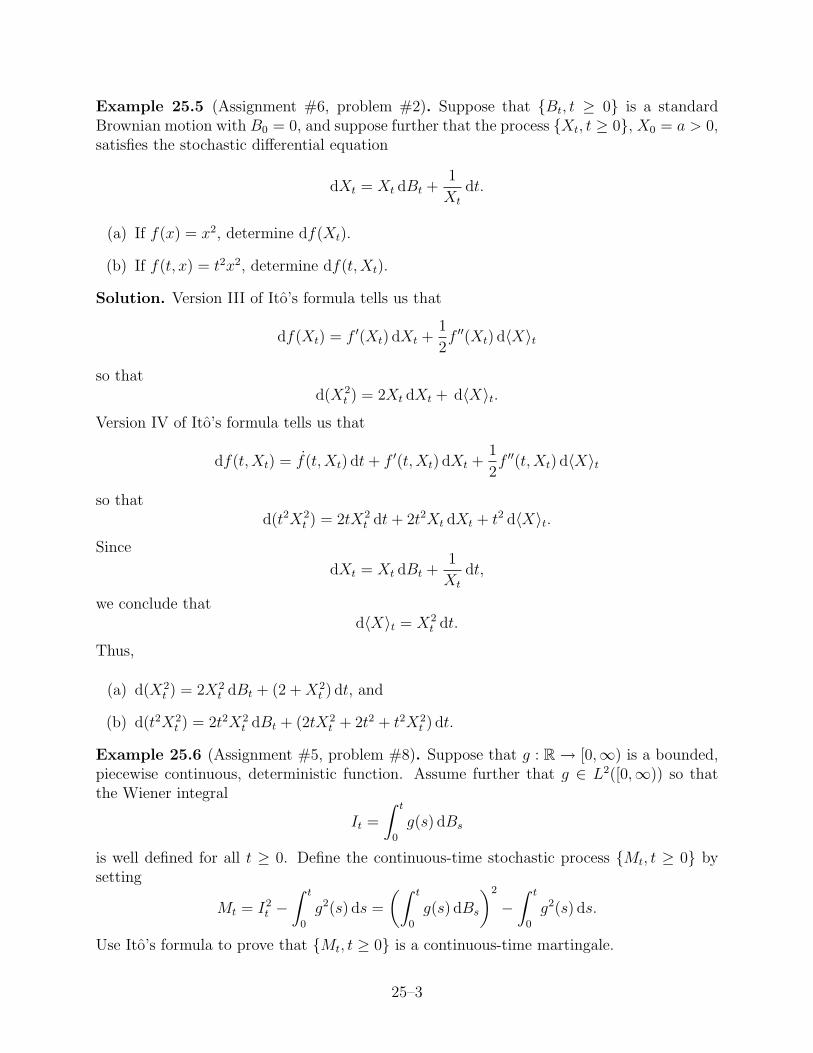
Example 25.5 (Assignment #6, problem #2). Suppose that Bt, t ≥ 0 is a standardBrownian motion with B0 = 0, and suppose further that the process Xt, t ≥ 0, X0 = a > 0,satisfies the stochastic differential equation
dXt = Xt dBt +1
Xt
dt.
(a) If f(x) = x2, determine df(Xt).
(b) If f(t, x) = t2x2, determine df(t,Xt).
Solution. Version III of Ito’s formula tells us that
df(Xt) = f ′(Xt) dXt +1
2f ′′(Xt) d〈X〉t
so thatd(X2
t ) = 2Xt dXt + d〈X〉t.
Version IV of Ito’s formula tells us that
df(t,Xt) = f(t,Xt) dt + f ′(t,Xt) dXt +1
2f ′′(t,Xt) d〈X〉t
so thatd(t2X2
t ) = 2tX2t dt + 2t2Xt dXt + t2 d〈X〉t.
Since
dXt = Xt dBt +1
Xt
dt,
we conclude thatd〈X〉t = X2
t dt.
Thus,
(a) d(X2t ) = 2X2
t dBt + (2 + X2t ) dt, and
(b) d(t2X2t ) = 2t2X2
t dBt + (2tX2t + 2t2 + t2X2
t ) dt.
Example 25.6 (Assignment #5, problem #8). Suppose that g : R → [0,∞) is a bounded,piecewise continuous, deterministic function. Assume further that g ∈ L2([0,∞)) so thatthe Wiener integral
It =
∫ t
0
g(s) dBs
is well defined for all t ≥ 0. Define the continuous-time stochastic process Mt, t ≥ 0 bysetting
Mt = I2t −
∫ t
0
g2(s) ds =
(∫ t
0
g(s) dBs
)2
−∫ t
0
g2(s) ds.
Use Ito’s formula to prove that Mt, t ≥ 0 is a continuous-time martingale.
25–3

Solution. If
It =
∫ t
0
g(s) dBs,
then dIt = g(t) dBt so that d〈I〉t = g2(t) dt. If
Mt = I2t −
∫ t
0
g2(s) ds,
then written in differential form we have
dMt = d(I2t )− g2(t) dt.
Version III of Ito’s formula implies
d(I2t ) = 2It dIt + d〈I〉t.
Substituting back therefore gives
dMt = d(I2t )− g2(t) dt = 2It dIt + d〈I〉t − g2(t) dt = 2g(t)It dBt + g2(t) dt− g2(t) dt
= 2g(t)It dBt.
Since Ito integrals are martingales, we conclude that Mt, t ≥ 0 is a continuous-time mar-tingale.
Example 25.7 (Assignment #5, problem #10). Suppose that Xt, t ≥ 0 is a time-inhomogeneous Ornstein-Uhlenbeck-type process defined by the SDE
dXt = σ(t) dBt − a(Xt − g(t)) dt
where g and σ are (sufficiently regular) deterministic functions of time. If Yt = expXt +ct,use Ito’s formula to compute dYt.
Solution. If dXt = σ(t) dBt − a(Xt − g(t)) dt and Yt = expXt + ct, then Version IV ofIto’s formula implies that
dYt = cYt dt + Yt dXt +Yt
2d〈X〉t.
Sinced〈X〉t = σ2(t)dt,
we conclude thatdYt
Yt
= σ(t) dBt +
[c− a(Xt − g(t)) +
σ2(t)
2
]dt.
Since we want a stochastic differential equation for Yt, we should really substitute back forXt in terms of Yt. Solving Yt = expXt + ct for Xt gives Xt = log(Yt)− ct so that
dYt
Yt
= σ(t) dBt +
[c− a(log(Yt)− ct− g(t)) +
σ2(t)
2
]dt
= σ(t) dBt +
[c(1 + at)− a log(Yt) + ag(t) +
σ2(t)
2
]dt.
25–4

Statistics 441 (Winter 2009) March 11, 2009Prof. Michael Kozdron
Lecture #26: Review
Example 26.1 (Assignment #5, problem #3). Suppose that the price of a stock Xt, t ≥ 0follows geometric Brownian motion with drift 0.05 and volatility 0.3 so that it satisfies thestochastic differential equation
dXt = 0.3Xt dBt + 0.05Xt dt.
If the price of the stock at time 2 is 30, determine the probability that the price of the stockat time 2.5 is between 30 and 33.
Solution. Since the price of the stock is given by geometric Brownian motion
dXt = 0.3Xt dBt + 0.05Xt dt,
we can read off the solution, namely
Xt = X0 exp
0.3Bt +
(0.05− 0.32
2
)t
= X0 exp0.30Bt + 0.005t.
Therefore,
P30 ≤ X2.5 ≤ 33|X2 = 30
= P
log(
30X0
)− 0.0125
0.30≤ B2.5 ≤
log(
33X0
)− 0.0125
0.30
∣∣∣∣B2 =log(
30X0
)− 0.01
0.30
= P
log(
30X0
)− 0.0125
0.30−
log(
30X0
)− 0.01
0.30≤ B0.5 ≤
log(
33X0
)− 0.0125
0.30−
log(
30X0
)− 0.01
0.30
= P
−0.0025
0.30≤ B0.5 ≤
log(
3330
)− 0.0025
0.30
using the stationarity of Brownian increments. If Z ∼ N (0, 1) so that B0.5 ∼√
0.5 Z, then
P −0.00833 ≤ B0.5 ≤ 0.3094 = P−0.0118 ≤ Z ≤ 0.4375 = 0.1587.
Remark. The solution to the previous exercise can be generalized as follows. Suppose thatXt, t ≥ 0 is geometric Brownian motion given by
dXt = σXt dBt + µXt dt
so that
Xt = X0 exp
σBt +
(µ− σ2
2
)t
.
26–1

If s ≥ 0, t > 0, then
log
(Xt+s
Xs
)= σ(Bt+s −Bs) +
(µ− σ2
2
)t.
Using the facts that (i) Bt+s − Bs is independent of Bs, and (ii) Bt+s − Bs ∼ Bt ∼ N (0, t)implies that (i) log (Xt+s/Xs) is independent of log Xs, and (ii)
log
(Xt+s
Xs
)∼(
Xt
X0
)∼ N
((µ− σ2
2
)t , σ2t
).
Therefore, we can conclude that if 0 < a < b and c > 0 are constants, then
Pa ≤ Xt+s ≤ b|Xs = c = P
log(a
c
)≤ log
(Xt+s
Xs
)≤ log
(b
c
)= P
log(a
c
)≤ log
(Xt
X0
)≤ log
(b
c
)
= P
log(
ac
)−(µ− σ2
2
)t
σ√
t≤ Z ≤
log(
bc
)−(µ− σ2
2
)t
σ√
t
where Z ∼ N (0, 1).
Example 26.2 (Assignment #5, problem #4). Consider the Ito process Xt, t ≥ 0 de-scribed by the stochastic differential equation
dXt = 0.10Xt dBt + 0.25Xt dt.
Calculate the probability that Xt is at least 5% higher than X0
(a) at time t = 0.01, and
(b) at time t = 1.
Solution. Since the price of the stock is given by geometric Brownian motion
dXt = 0.25Xt dt + 0.10Xt dBt,
we can read off the solution, namely
Xt = X0 exp
0.10Bt +
(0.25− 0.102
2
)t
= X0 exp0.10Bt + 0.245t.
Therefore, if Z ∼ N (0, 1), then
PXt ≥ 1.05X0 = P
Bt ≥
log(1.05)− 0.245t
0.10
= P
Z ≥ log(1.05)− 0.245t
0.10√
t
.
(a) If t = 0.01, then PX0.01 ≥ 1.05X0 = PZ ≥ 4.634 = 0.000002.
(b) If t = 1, then PX1 ≥ 1.05X0 = PZ ≥ −1.962 = 0.9751.
26–2

Example 26.3 (Assignment #5, problem #5). Consider the Ito process Xt, t ≥ 0 de-scribed by the stochastic differential equation
dXt = 0.05Xt dBt + 0.1Xt dt, X0 = 35.
Compute PX5 ≤ 48.
Solution. Since the price of the stock is given by geometric Brownian motion
dXt = 0.1Xt dt + 0.05Xt dBt, X0 = 35,
we can read off the solution, namely
Xt = 35 exp
0.05Bt +
(0.1− 0.052
2
)t
= 35 exp0.05Bt + 0.09875t.
Therefore, if Z ∼ N (0, 1), then
PX5 ≤ 48 = PB5 ≤ −3.5579 = P
Z ≤ −3.5579√
5
= PZ ≤ −1.5911 = 0.0558.
Example 26.4 (Assignment #5, problem #7; Assignment #7, problem #5). Suppose thatthe diffusion Xt, t ≥ 0 is defined by the SDE
dXt = σ(t)Xt dBt + µ(t)Xt dt
where σ(t) and µ(t) are deterministic functions of time. If we consider log Xt, then Ito’sformula implies
d log Xt =1
Xt
dXt −1
2X2t
d〈X〉t.
Since d〈X〉t = σ2(t)X2t dt, we conclude
d log Xt = σ(t) dBt + µ(t) dt− 1
2σ2(t) dt = σ(t) dBt +
(µ(t)− 1
2σ2(t)
)dt.
We can now integrate from 0 to t to find
log Xt − log X0 =
∫ t
0
σ(s) dBs +
∫ t
0
(µ(s)− 1
2σ2(s)
)ds.
Solving for Xt gives
Xt = X0 exp
∫ t
0
σ(s) dBs +
∫ t
0
(µ(s)− σ2(s)
2
)ds
.
26–3

Statistics 441 (Winter 2009) March 13, 2009Prof. Michael Kozdron
Lecture #27: Risk Neutrality
We will now use the Feynman-Kac representation theorem to derive a general solution to theBlack-Scholes option pricing problem for European call options. This representation of thesolution will be needed next lecture when we explain how to use the characteristic functionof a diffusion to price an option.
Suppose that the asset price process St, t ≥ 0 satisfies the stochastic differential equation
dSt = σ(t, St)St dBt + µ(t, St)St dt, (27.1)
or equivalently,dSt
St
= σ(t, St) dBt + µ(t, St) dt,
where Bt, t ≥ 0 is a standard Brownian motion with B0 = 0, and that the risk-freeinvestment D(t, St) evolves according to
dD(t, St) = rD(t, St) dt
where r > 0 is the risk-free interest rate.
Remark. We are writing Bt, t ≥ 0 for the Brownian motion that drives the asset priceprocess since the formula that we are going to derive for the fair price at time t = 0 of aEuropean call option on this asset involves a one-dimensional Brownian motion distinct fromthis one.
Remark. The asset price process given by (27.1) is similar to geometric Brownian motion,except that the volatility and drift do not necessarily need to be constant. Instead, they canbe stochastic, but the randomness is assumed to come from the asset price itself. In thisgeneral form, there is no explicit form for St, t ≥ 0 as the solution of the SDE (27.1).
Suppose further that we write V (t, St), 0 ≤ t ≤ T , to denote the price at time t of a Europeancall option with expiry date T on the asset St, t ≥ 0. If the payoff function is given byΛ(x), x ∈ R, then
V (T, ST ) = Λ(ST ).
(Recall that a European call option can be exercised only on the expiry date T and notearlier.) Our goal is to determine V (0, S0), the fair price to pay at time t = 0.
Furthermore, assume that there are no arbitrage opportunities so that there exists a replic-ating portfolio
Π(t, St) = A(t, St)St + D(t, St)
consisting of a cash deposit D and a number A of assets which is self-financing:
dΠ(t, St) = A(t, St) dSt + rD(t, St) dt.
27–1

As in Lecture #17, this implies that the change in V (t, St)−Π(t, St) over any time step is non-random and must equal the corresponding growth offered by the continuously compoundedrisk-free interest rate. That is,
d[V (t, St)− Π(t, St)
]= r[V (t, St)− Π(t, St)
]dt.
By repeating the calculations in Lecture #17 assuming that the asset price movement satis-fies (27.1) leads to the following conclusion. The function V (t, x), 0 ≤ t ≤ T , x ∈ R, satisfiesthe Black-Scholes partial differential equation
V (t, x) +σ2(t, x)
2x2V ′′(t, x) + rxV ′(t, x)− rV (t, x) = 0, 0 ≤ t ≤ T, x ∈ R, (27.2)
subject to the terminal conditionV (T, x) = Λ(x).
Note. The only difference between (27.2) and the Black-Scholes PDE that we derived inLecture #17, namely (17.10), is the appearance of the function σ(t, x) instead of the constantσ. Thus, (27.2) reduces to (17.10) when σ(t, x) = σ is constant.
At this point, we observe that the formulation of the option pricing problem sounds rathersimilar to the formulation of the Feynman-Kac representation theorem which we now recall.
Theorem 27.1 (Feynman-Kac Representation Theorem). Suppose that u ∈ C2(R), and letXt, t ≥ 0 be defined by the SDE
dXt = a(t,Xt) dBt + b(t,Xt) dt.
The unique bounded function f : [0,∞)× R → R satisfying the partial differential equation
(Af)(t, x) = b(t, x)f ′(t, x) +1
2a2(t, x)f ′′(t, x) + f(t, x) = 0, 0 ≤ t ≤ T, x ∈ R, (27.3)
subject to the terminal condition
f(T, x) = u(x), x ∈ R,
is given byf(t, x) = E[u(XT )|Xt = x].
However, the differential equation (27.2) that we need to solve is of the form
b(t, x)g′(t, x) +1
2a2(t, x)g′′(t, x) + g(t, x) = rg(t, x), 0 ≤ t ≤ T, x ∈ R, (27.4)
subject to the terminal condition
g(T, x) = u(x), x ∈ R.
27–2

In other words, we need to solve a non-homogeneous partial differential equation. Althoughthe theory for non-homogeneous PDEs is reasonably well-established, it is not too difficultto guess what the solution to our particular equation (27.4) must be. If we let
g(t, x) = e−r(T−t)f(t, x), 0 ≤ t ≤ T, x ∈ R,
where f(t, x) satisfies the homogeneous partial differential equation (Af)(t, x) = 0 givenin (27.3), then g(T, x) = f(T, x) = u(x), and
g′(t, x) = e−r(T−t)f ′(t, x), g′′(t, x) = e−r(T−t)f ′′(t, x), and
g(t, x) = e−r(T−t)f(t, x) + re−r(T−t)f(t, x)
so that
b(t, x)g′(t, x) +1
2a2(t, x)g′′(t, x) + g(t, x)
= b(t, x)e−r(T−t)f ′(t, x) +1
2a2(t, x)e−r(T−t)f ′′(t, x) + e−r(T−t)f(t, x) + re−r(T−t)f(t, x)
= e−r(T−t)
[b(t, x)f ′(t, x) +
1
2a2(t, x)f ′′(t, x) + f(t, x)
]+ re−r(T−t)f(t, x)
= e−r(T−t)(Af)(t, x) + rg(t, x)
= rg(t, x)
using the assumption that (Af)(t, x) = 0. In other words, we have established the followingextension of the Feynman-Kac representation theorem.
Theorem 27.2 (Feynman-Kac Representation Theorem). Suppose that u ∈ C2(R), and letXt, t ≥ 0 be defined by the SDE
dXt = a(t,Xt) dBt + b(t,Xt) dt.
The unique bounded function g : [0,∞)× R → R satisfying the partial differential equation
b(t, x)g′(t, x) +1
2a2(t, x)g′′(t, x) + g(t, x)− rg(t, x) = 0, 0 ≤ t ≤ T, x ∈ R,
subject to the terminal condition
g(T, x) = u(x), x ∈ R,
is given byg(t, x) = e−r(T−t)E[u(XT )|Xt = x].
At this point, let’s recall where we are. We are assuming that the asset price St, t ≥ 0evolves according to
dSt = σ(t, St)St dBt + µ(t, St)St dt
27–3

and we want to determine V (0, S0), the fair price at time t = 0 of a European call optionwith expiry date T and payoff V (T, ST ) = Λ(ST ) where Λ(x), x ∈ R, is given. We have alsoshown that V (t, x) satisfies the PDE
V (t, x) +σ2(t, x)
2x2V ′′(t, x) + rxV ′(t, x)− rV (t, x) = 0, 0 ≤ t ≤ T, x ∈ R, (27.5)
subject to the terminal conditionV (T, x) = Λ(x).
The generalized Feynman-Kac representation theorem tells us that the solution to
b(t, x)g′(t, x) +1
2a2(t, x)g′′(t, x) + g(t, x)− rg(t, x) = 0, 0 ≤ t ≤ T, x ∈ R, (27.6)
subject to the terminal condition g(T, x) = Λ(x) is
g(t, x) = e−r(T−t)E[Λ(XT )|Xt = x], (27.7)
where Xt satisfies the SDE
dXt = a(t,Xt) dBt + b(t,Xt) dt
and Bt, t ≥ 0 is a standard one-dimensional Brownian motion with B0 = 0. Note thatthe expectation in (27.7) is with respect to the process Xt, t ≥ 0 driven by the Brownianmotion Bt, t ≥ 0.Comparing (27.5) and (27.6) suggests that
b(t, x) = rx and a2(t, x) = σ2(t, x)x2
so thatdXt = σ(t,Xt)Xt dBt + rXt dt, (27.8)
or equivalently,dXt
Xt
= σ(t,Xt) dBt + r dt,
Hence, we have developed a complete solution to the European call option pricing problemwhich we summarize in Theorem 27.3 below.
Remark. The process Xt, t ≥ 0 defined by the SDE (27.8) is sometimes called the risk-neutral process associated with the asset price process St, t ≥ 0 defined by (27.1). As withthe asset price process, the associated risk-neutral process is similar to geometric Brownianmotion. Note that the function σ(t, x) is the same in both equations. However, Bt, t ≥ 0,the Brownian motion that drives St, t ≥ 0 is NOT the same as Bt, t ≥ 0, the Brownianmotion that drives Xt, t ≥ 0.
Remark. The approach we have used to develop the associated risk-neutral process wasvia the Feynman-Kac representation theorem. An alternative approach which we do notdiscuss is to use the Girsanov-Cameron-Martin theorem to construct an equivalent martingalemeasure.
27–4

Theorem 27.3. Let V (t, St), 0 ≤ t ≤ T , denote the fair price to pay at time t of a Europeancall option having payoff V (T, ST ) = Λ(ST ) on the asset price St, t ≥ 0 which satisfies thestochastic differential equation
dSt = σ(t, St)St dBt + µ(t, St)St dt
where Bt, t ≥ 0 is a standard Brownian motion with B0 = 0. The fair price to pay at timet = 0 is given by
V (0, S0) = e−rT E[Λ(XT )|X0 = S0]
where the associated risk-neutral process Xt, t ≥ 0 satisfies the stochastic differential equa-tion
dXt = σ(t,Xt)Xt dBt + rXt dt
and Bt, t ≥ 0 is a standard one-dimensional Brownian motion distinct from Bt, t ≥ 0.
Remark. Since S0, the value of the underlying asset at t = 0, is known, in order to calculatethe expectation E[Λ(XT )|X0 = S0], you need to know something about the distribution ofXT . There is no general formula for determining the distribution of XT in terms of thedistribution of ST unless some additional structure is known about σ(t, x). For instance,assuming that σ(t, x) = σ is constant leads to the Black-Scholes formula from Lecture #18,while assuming σ(t, x) = σ(t) is a deterministic function of time leads to an explicit formulawhich, though similar, is more complicated to write down.
Example 27.4. We now explain how to recover the Black-Scholes formula in the case thatSt, t ≥ 0 is geometric Brownian motion and Λ(x) = (x−E)+. Since the asset price processSDE is
dSt = σSt dBt + µSt dt
we conclude that the risk-neutral process is
dXt = σXt dBt + rXt dt.
The risk-neutral process is also geometric Brownian motion (but with drift r) so that
XT = X0 exp
σBT +
(r − σ2
2
)T
= S0 exp
σBT +
(r − σ2
2
)T
since we are assuming that X0 = S0. Since BT ∼ N (0, T ), we can write
XT = S0 exp
(r − σ2
2
)T
exp
σ√
TZ
for Z ∼ N (0, 1). Therefore,
V (0, S0) = e−rT E[Λ(XT )|X0 = S0] = e−rT E[(XT − E)+|X0 = S0]
can be evaluated using Exercise 4.7, namely if a > 0, b > 0, c > 0 are constants andZ ∼ N (0, 1), then
E[ (aebZ − c)+ ] = aeb2/2 Φ
(b +
1
blog
a
c
)− c Φ
(1
blog
a
c
),
27–5
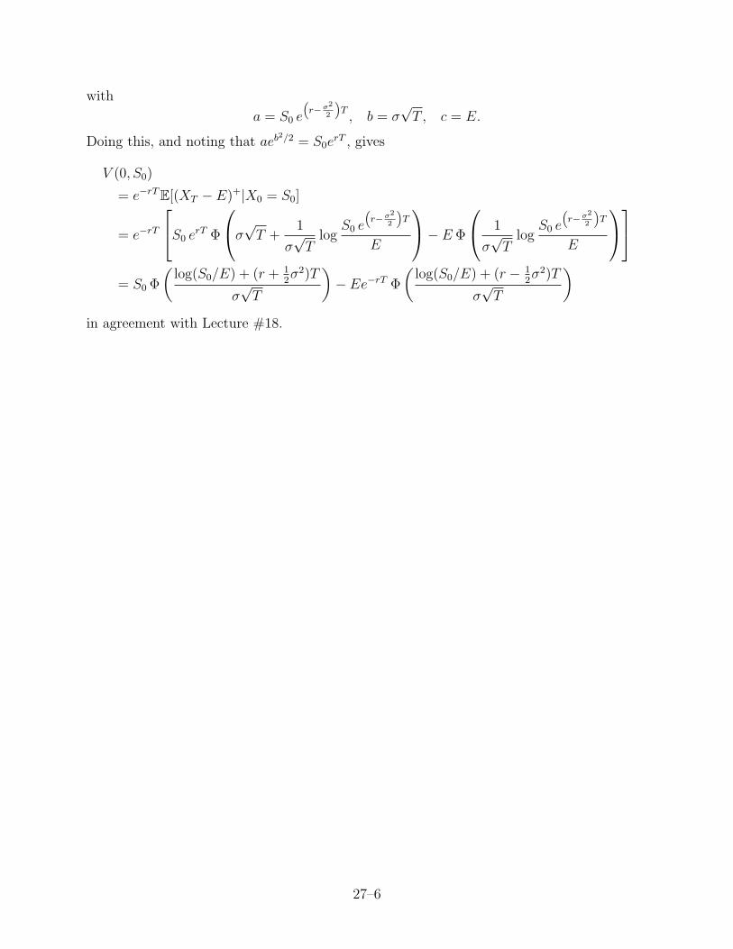
with
a = S0 e
“r−σ2
2
”T, b = σ
√T , c = E.
Doing this, and noting that aeb2/2 = S0erT , gives
V (0, S0)
= e−rT E[(XT − E)+|X0 = S0]
= e−rT
S0 erT Φ
σ√
T +1
σ√
Tlog
S0 e
“r−σ2
2
”T
E
− E Φ
1
σ√
Tlog
S0 e
“r−σ2
2
”T
E
= S0 Φ
(log(S0/E) + (r + 1
2σ2)T
σ√
T
)− Ee−rT Φ
(log(S0/E) + (r − 1
2σ2)T
σ√
T
)in agreement with Lecture #18.
27–6

Statistics 441 (Winter 2009) March 16, 2009Prof. Michael Kozdron
Lecture #28: A Numerical Approach to Option Pricing UsingCharacteristic Functions
As we discussed in Lectures #22 and #23, it is sometimes possible to determine the charac-teristic function ϕXT
(θ) for the random variable XT , which is defined via a diffusion. We thendiscussed risk-neutrality in Lecture #27, and derived a complete solution to the problem ofpricing European call options.
At this point, it is time to address the following question. How does knowing the character-istic function help us determine the value of an option?
In order to keep our notation straight, we will write St, t ≥ 0 for the underlying asset priceprocess driven by the Brownian motion Bt, t ≥ 0, and we will assume that
dSt
St
= σ(t, St) dBt + µ(t, St) dt.
We will then write Xt, t ≥ 0 for the associated risk-neutral process driven by the Brownianmotion Bt, t ≥ 0. Guided by Lecture #27, we will phrase all of our results in terms of therisk-neutral process Xt, t ≥ 0.
Note. The purpose of Example 22.4 with arithmetic Brownian motion and Example 22.5with the Ornstein-Uhlenbeck process was to illustrate how the characteristic function couldbe found without actually solving the SDE. Of course, neither of these is an adequate model ofthe asset price movement. Heston’s model, however, is an adequate model for the underlyingasset price, and in Lecture 23 we found the characteristic function without solving thedefining SDE.
Suppose that we are interested in determining the fair price at time t = 0 of a Europeancall option on the asset price St, t ≥ 0 with strike price E and expiry date T assuminga risk-free interest rate r. The payoff function is therefore Λ(x) = (x − E)+. If V (0, S0)denotes the fair price at time t = 0, then from Theorem 27.3, we can express the solution as
V (0, S0) = e−rT E[(XT − E)+|X0 = S0]
where the expectation is with respect to the associated risk-neutral process Xt, t ≥ 0driven by the Brownian motion Bt, t ≥ 0. As we saw in Lecture #27, the associatedrisk-neutral process is a geometric-type Brownian motion given by
dXt
Xt
= σ(t,Xt) dBt + r dt.
It turns out that for the following calculations it is more convenient to consider the processZt, t ≥ 0 where
Zt = log Xt.
28–1

Exercise 28.1. Suppose that Xt, t ≥ 0 satisfies the associated risk-neutral SDE
dXt = σ(t,Xt)Xt dBt + rXt dt.
Use Ito’s formula to determine the SDE satisfied by Zt, t ≥ 0 where Zt = log Xt.
We will now write the strike price E as ek (so that k = log E) and XT = eZT . Therefore,
V (0, S0) = e−rT E[(XT − E)+|X0 = S0] = e−rT E[(eZT − ek)+]
where Z0 = log X0 = log S0 is known.
Suppose further that we are able to determine the density function of the random variableZT which we write as fZT
(z) so that
V (0, S0) = e−rT E[(eZT − ek)+] = e−rT
∫ ∞
−∞(ez − ek)+fZT
(z) dz = e−rT
∫ ∞
k
(ez − ek)fZT(z) dz.
We will now view the fair price at time 0 as a function of the logarithm of the strike price kso that
V (k) = e−rT
∫ ∞
k
(ez − ek)fZT(z) dz.
As k → −∞ (so that E → 0) we see that V (k) → S0 which implies that V (k) is notintegrable: ∫ ∞
−∞V (k) dk does not exist.
It necessarily follows that V (k) is not square-integrable:∫ ∞
−∞V 2(k) dk does not exist.
However, if we considerW (k) = eckV (k), (28.1)
then W is square-integrable for a suitable c > 0 which may depend on the model forSt, t ≥ 0. The Fourier transform of W is the function W defined by
W (ξ) =
∫ ∞
−∞eiξkW (k) dk. (28.2)
Remark. The existence of the Fourier transform requires that the function W (k) be in L2.
Therefore, substituting in for W (k) gives
W (ξ) = e−rT
∫ ∞
−∞
∫ ∞
k
eiξkeck(ez − ek)fZT(z) dz dk
= e−rT
∫ ∞
−∞
∫ ∞
k
(eze(iξ+c)k − e(iξ+c+1)k
)fZT
(z) dz dk.
28–2

Switching the order of integration, we find
W (ξ) = e−rT
∫ ∞
−∞fZT
(z)
∫ z
−∞
(eze(iξ+c)k − e(iξ+c+1)k
)dk dz.
Since ∫ z
−∞
(eze(iξ+c)k − e(iξ+c+1)k
)dk =
eze(iξ+c)z
iξ + c− e(iξ+c+1)z
iξ + c + 1=
e(iξ+c+1)z
(iξ + c)(iξ + c + 1),
we conclude that
W (ξ) = e−rT
∫ ∞
−∞fZT
(z)e(iξ+c+1)z
(iξ + c)(iξ + c + 1)dz
=e−rT
(iξ + c)(iξ + c + 1)
∫ ∞
−∞e(iξ+c+1)zfZT
(z) dz
=e−rT
(iξ + c)(iξ + c + 1)
∫ ∞
−∞ei(ξ−i(c+1))zfZT
(z) dz
=e−rT
(iξ + c)(iξ + c + 1)E[ei(ξ−i(c+1))ZT ]
=e−rT
(iξ + c)(iξ + c + 1)ϕZT
(ξ − i(c + 1)). (28.3)
Remark. It can be shown that a sufficient condition for W (k) to be square-integrable is forW (0) to be finite. This is equivalent to
E(Sc+1T ) < ∞.
The choice c = 0.75 can be shown to work for the Heston model.
Given the Fourier transform W (ξ), one recovers the original function W (k) via the inverseFourier transform defined by
W (k) =1
π
∫ ∞
0
e−iξkW (ξ) dξ. (28.4)
Substituting (28.1) and (28.3) into (28.4) implies
eckV (k) =1
π
∫ ∞
0
e−iξk e−rT
(iξ + c)(iξ + c + 1)ϕZT
(ξ − i(c + 1)) dξ
so that
V (0, S0) = V (k) =e−cke−rT
π
∫ ∞
0
e−iξk
(iξ + c)(iξ + c + 1)ϕZT
(ξ − i(c + 1)) dξ (28.5)
is the fair price at time t = 0 of a European call option with strike price E = ek and expirydate T assuming the risk-free interest rate is r > 0.
28–3

Remark. Notice that (28.5) expresses the required price of a European call option in termsof ϕZT
(θ), the characteristic function of ZT = log XT , the logarithm of XT defined via therisk-neutral SDE. The usefulness of this formula is that it can be approximated numericallyin an extremely efficient manner using the fast Fourier transform (FFT). In fact, it is shownin [23] that the FFT approach to option pricing for Heston’s model is over 300 times fasterthan by pricing options using Monte Carlo simulations. There are, however, a number ofother practical issues to implementation that the FFT approach to option pricing raises; forfurther details, see [23].
Example 28.2. The Heston model assumes that the asset price process St, t ≥ 0 satisfiesthe SDE
dSt =√
vt St dB(1)t + µSt dt
where the variance process vt, t ≥ 0 satisfies
dvt = σ√
vt dB(2)t + a(b− vt) dt
and the two driving Brownian motions B(1)t , t ≥ 0 and B(2)
t , t ≥ 0 are correlated withrate ρ, i.e.,
d〈B(1), B(2)〉t = ρ dt.
Although this is a two-dimensional example, the risk-neutral process can be worked out ina similar manner to the one-dimensional case. The result is that
dXt =√
vt Xt dB(1)t + rXt dt.
If we now considerZt = log(Xt),
thendZt =
√vt dB
(1)t +
(r − vt
2
)dt,
and so
ϕZT(θ)
exp
iθx− (iθ+θ2)y
γ coth γT2
+(a−iσρθ)+ abT (a−iσρθ)
σ2 + iθrT
(cosh γT
2+ a−iσρθ
γsinh γT
2
) 2abσ2
where x = Z0 = log(X0) and y = v0.
28–4

Statistics 441 (Winter 2009) March 23, 2009Prof. Michael Kozdron
Lecture #29: An Introduction to Functional Analysis forFinancial Applications
For the remainder of the course, we are going to discuss some approaches to risk analysis.We will do this, however, with some formality. As such, we need to learn a little bit offunctional analysis.
In calculus, we analyze individual functions and study particular properties of these indi-vidual functions.
Example 29.1. Consider the function f(x) = x2. We see that the domain of f is all realnumbers, and the range of f is all non-negative real numbers. The graph of f is a parabolawith its vertex at (0, 0) and opening up. We can also compute
f ′(x) =d
dxx2 = 2x and
∫f(x) dx =
∫x2 dx =
x3
3+ C.
In functional analysis we study sets of functions with a view to properties possessed by everyfunction in the set. Actually, you would have seen a glimpse of this in calculus.
Example 29.2. Let X be the set of all differentiable functions with domain R. If f ∈ X ,then f is necessarily (i) continuous, and (ii) Riemann integrable on every finite interval [a, b].
In order to describe a function acting on a set of functions such as X in the previous example,we use the word functional (or operator).
Example 29.3. As in the previous example, let X denote the set of differentiable functionson R. Define the functional D by setting D(f) = f ′ for f ∈ X . That is,
f ∈ X 7→ f ′.
Formally, we define D by(Df)(x) = f ′(x)
for every x ∈ R, f ∈ X .
Example 29.4. We have already seen a number of differential operators in the context ofthe Feynman-Kac representation theorem. If we let X denote the space of all functions f oftwo variables, say f(t, x), such that f ∈ C1([0,∞))×C2(R), and a(t, x) and b(t, x) are givenfunctions, then we can define the functional A by setting
(Af)(t, x) = b(t, x)f ′(t, x) +1
2a2(t, x)f ′′(t, x) + f(t, x).
The next definition is of fundamental importance to functional analysis.
29–1

Definition 29.5. Let X be a space. A norm on X is a function(al) ||·|| : X → R satisfyingthe following properties:
(a) ||x|| ≥ 0 for every x ∈ X ,
(b) ||x|| = 0 if and only if x = 0,
(c) ||αx|| = |α|||x|| for every α ∈ R and x ∈ X , and
(d) ||x + y|| ≤ ||x||+ ||y|| for every x, y ∈ X .
Remark. We often call (d) the triangle inequality.
Example 29.6. The idea of a norm is that it generalizes the usual absolute value on R.Indeed, let X = R and for x ∈ X define ||x|| = |x|. Properties of absolute value immediatelyimply that
(a) ||x|| = |x| ≥ 0 for every x ∈ X ,
(b) ||x|| = |x| = 0 if and only if x = 0, and
(c) ||αx|| = |αx| = |α||x| = |α|||x|| for every α ∈ R and x ∈ X .
The triangle inequality |x + y| ≤ |x| + |y| is essentially a fact about right-angle triangles.The proof is straightforward. Observe that xy ≤ |x||y|. Therefore,
x2 + 2xy + y2 ≤ x2 + 2|x||y|+ y2 or, equivalently, (x + y)2 ≤ x2 + 2|x||y|+ y2.
Using the fact that x2 = |x|2 implies
|x + y|2 ≤ |x|2 + 2|x||y|+ |y|2 = (|x|+ |y|)2.
Taking square roots of both sides yields the result.
Exercise 29.7. Assume that x, y ∈ R. Show that the triangle inequality |x + y| ≤ |x|+ |y|is equivalent to the following statements:
(i) |x− y| ≤ |x|+ |y|,
(ii) |x + y| ≥ |x| − |y|,
(iii) |x− y| ≥ |x| − |y|, and
(iii) |x− y| ≥ |y| − |x|.
Example 29.8. Let X = R2. If x ∈ R2, we can write x = (x1, x2). If we define
||x|| =√
x21 + x2
2,
then ||·|| is a norm on X .
29–2

Exercise 29.9. Verify that ||x|| =√
x21 + x2
2 is, in fact, a norm on R2.
Example 29.10. More generally, let X = Rn. If x ∈ Rn, we can write x = (x1, . . . , xn). Ifwe define
||x|| =√
x21 + · · ·+ x2
n,
then ||·|| is a norm on X .
Example 29.11. Let X denote the space of continuous functions on [0, 1]. In calculus, wewould write such a function as f(x), 0 ≤ x ≤ 1. In functional analysis, we prefer to writesuch a function as x(t), 0 ≤ t ≤ 1. That is, it is traditional to use a lower case x to denotean arbitrary point in a space. It so happens that our space X consists of individual pointsx which happen themselves to be functions. If we define
||x|| = max0≤t≤1
|x(t)|,
then ||·|| is a norm on X . Indeed,
(a) |x(t)| ≥ 0 for every 0 ≤ t ≤ 1 and x ∈ X so that ||x|| ≥ 0,
(b) ||x|| = 0 if and only if x(t) = 0 for every 0 ≤ t ≤ 1 (i.e., x = 0), and
(c) ||αx|| = max0≤t≤1
|αx(t)| = |α| max0≤t≤1
|x(t)| = |α|||x|| for every α ∈ R and x ∈ X .
As for (d), notice that
||x + y|| = max0≤t≤1
|x(t) + y(t)| ≤ max0≤t≤1
(|x(t)|+ |y(t)|)
by the usual triangle inequality. Since
max0≤t≤1
(|x(t)|+ |y(t)|) ≤ max0≤t≤1
|x(t)|+ max0≤t≤1
|y(t)| = ||x||+ ||y||,
we conclude ||x + y|| ≤ ||x|| + ||y|| as required. Note that we sometimes write C[0, 1] for thespace of continuous functions on [0, 1].
Example 29.12. Let X denote the space of all random variables with finite variance. Inkeeping with the traditional notation for random variables, we prefer to write X ∈ X insteadof the traditional functional analysis notation x ∈ X . As we will see next lecture, if we define
||X|| =√
E(X2),
then this defines a norm on X . (Actually, this is not quite precise. We will be more carefulnext lecture.) A risk measure will be a functional ρ : X → R satisfying certain naturalproperties.
29–3
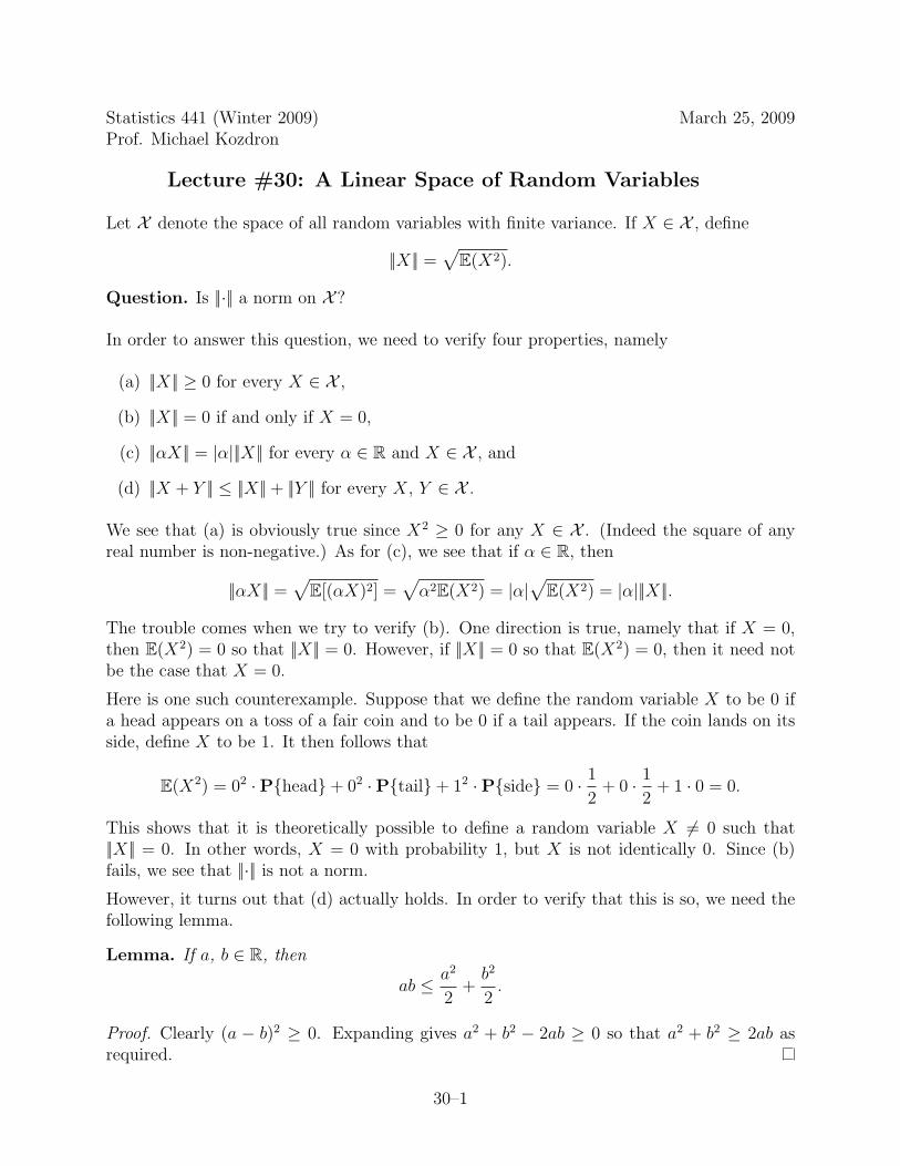
Statistics 441 (Winter 2009) March 25, 2009Prof. Michael Kozdron
Lecture #30: A Linear Space of Random Variables
Let X denote the space of all random variables with finite variance. If X ∈ X , define
||X|| =√
E(X2).
Question. Is ||·|| a norm on X ?
In order to answer this question, we need to verify four properties, namely
(a) ||X|| ≥ 0 for every X ∈ X ,
(b) ||X|| = 0 if and only if X = 0,
(c) ||αX|| = |α|||X|| for every α ∈ R and X ∈ X , and
(d) ||X + Y || ≤ ||X||+ ||Y || for every X, Y ∈ X .
We see that (a) is obviously true since X2 ≥ 0 for any X ∈ X . (Indeed the square of anyreal number is non-negative.) As for (c), we see that if α ∈ R, then
||αX|| =√
E[(αX)2] =√
α2E(X2) = |α|√
E(X2) = |α|||X||.
The trouble comes when we try to verify (b). One direction is true, namely that if X = 0,then E(X2) = 0 so that ||X|| = 0. However, if ||X|| = 0 so that E(X2) = 0, then it need notbe the case that X = 0.
Here is one such counterexample. Suppose that we define the random variable X to be 0 ifa head appears on a toss of a fair coin and to be 0 if a tail appears. If the coin lands on itsside, define X to be 1. It then follows that
E(X2) = 02 ·Phead+ 02 ·Ptail+ 12 ·Pside = 0 · 1
2+ 0 · 1
2+ 1 · 0 = 0.
This shows that it is theoretically possible to define a random variable X 6= 0 such that||X|| = 0. In other words, X = 0 with probability 1, but X is not identically 0. Since (b)fails, we see that ||·|| is not a norm.
However, it turns out that (d) actually holds. In order to verify that this is so, we need thefollowing lemma.
Lemma. If a, b ∈ R, then
ab ≤ a2
2+
b2
2.
Proof. Clearly (a − b)2 ≥ 0. Expanding gives a2 + b2 − 2ab ≥ 0 so that a2 + b2 ≥ 2ab asrequired.
30–1
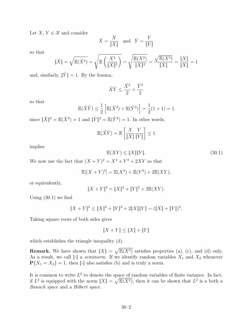
Let X, Y ∈ X and consider
X =X
||X||and Y =
Y
||Y ||so that
||X|| =
√E(X2) =
√E(
X2
||X||2
)=
√E(X2)
||X||2=
√E(X2)
||X||=||X||||X||
= 1
and, similarly, ||Y || = 1. By the lemma,
XY ≤ X2
2+
Y 2
2
so that
E(XY ) ≤ 1
2
[E(X2) + E(Y 2)
]=
1
2(1 + 1) = 1
since ||X||2 = E(X2) = 1 and ||Y ||2 = E(Y 2) = 1. In other words,
E(XY ) = E[
X
||X||Y
||Y ||
]≤ 1
impliesE(XY ) ≤ ||X||||Y ||. (30.1)
We now use the fact that (X + Y )2 = X2 + Y 2 + 2XY so that
E[(X + Y )2] = E(X2) + E(Y 2) + 2E(XY ),
or equivalently,||X + Y ||2 = ||X||2 + ||Y ||2 + 2E(XY ).
Using (30.1) we find
||X + Y ||2 ≤ ||X||2 + ||Y ||2 + 2||X||||Y || = (||X||+ ||Y ||)2.
Taking square roots of both sides gives
||X + Y || ≤ ||X||+ ||Y ||
which establishes the triangle inequality (d).
Remark. We have shown that ||X|| =√
E(X2) satisfies properties (a), (c), and (d) only.As a result, we call ||·|| a seminorm. If we identify random variables X1 and X2 wheneverPX1 = X2 = 1, then ||·|| also satisfies (b) and is truly a norm.
It is common to write L2 to denote the space of random variables of finite variance. In fact,if L2 is equipped with the norm ||X|| =
√E(X2), then it can be shown that L2 is a both a
Banach space and a Hilbert space.
30–2

Statistics 441 (Winter 2009) March 27, 2009Prof. Michael Kozdron
Lecture #31: Value at Risk
Suppose that Ω denotes the set of all possible financial scenarios up to a given expiry dateT . In other words, if we write St, t ≥ 0 to denote the underlying asset price process thatwe care about, then Ω consists of all possible trajectories on [0, T ]. We will abbreviate sucha trajectory simply by ω.
Therefore, we will let the random variable X denote our financial position at time T . Inother words, X : Ω → R is given by ω 7→ X(ω) where X(ω) describes our financial positionat time T (or our resulting net worth already discounted) assuming the trajectory ω wasrealized.
Our goal is to quantify the risk associated with the financial position X. Arbitrarily, wecould use Var(X) to measure risk. Although this is easy to work with, it is symmetric. Thisis not desirable in a financial context since upside risk is fine; it is perfectly acceptable tomake more money than expected!
As a first example, we will consider the so-called value at risk at level α. Recall that Xdenotes the space of all random variables of finite variance. As we saw in Lecture #30, ifwe define ||X|| =
√E(X2) for X ∈ X , then ||·|| defines a norm on X as long as we identify
random variables which are equal with probability one.
Example 31.1. Let X be a given financial position and suppose that α ∈ (0, 1). We willsay that X is acceptable if and only if
PX < 0 ≤ α.
We then define VaRα(X), the value at risk of the position X at level α ∈ (0, 1), to be
VaRα(X) = infm : PX + m < 0 ≤ α.
In other words, if X is not acceptable, then the value at risk is the minimal amount mof capital that is required to be added to X in order to make it acceptable. For instance,suppose that we declare X to be acceptable if PX < 0 ≤ 0.1. If X is known to have aN (1, 1) distribution, then X is not acceptable since PX < 0 = 0.1587. However, we find(accurate to 4 decimal places) that PX < −0.2816 = 0.1. Therefore, if X ∼ N (1, 1), then
VaR0.1(X) = infm : PX + m < 0 ≤ 0.1 = 0.2816.
Since X was not acceptable, we see that the minimal capital we must add to make it ac-ceptable is 0.2816. On the other hand, if X ∼ N (3, 1), then X is already acceptable andso
VaR0.1(X) = infm : PX + m < 0 ≤ 0.1 = −1.7184
since PX < 1.7184 = 0.1. Since X was already acceptable, our value at risk is negative.This indicates that we could afford to lower our capital by 1.7184 and our position would
31–1

still be acceptable. We can write VaRα(X) in terms of the distribution function FX of X asfollows. Let c = −m so that PX + m < 0 = PX − c < 0, and so
PX − c < 0 = PX < c = PX ≤ c −PX = c = FX(c−)
where c− denotes the limit from the left. Therefore,
VaRα(X) = inf−c : FX(c−) ≤ α = − supc : FX(c−) ≤ α.
Although value at risk is widely used, it has a number of drawbacks. For instance, it paysattention only to shortfalls (X < 0), but never to how bad they are. It may also penalizediversification. Mathematically, value at risk requires a probability measure P to be knownin advance, and it does not behave in a convex manner.
Exercise 31.2. Show that if X ≤ Y , then VaRα(X) ≥ VaRα(Y ).
Exercise 31.3. Show that if r ∈ R, then VaRα(X + r) = VaRα(X)− r.
As we will learn next lecture, any functional satisfying the properties given in the previoustwo exercises will be called a monetary risk measure. That is, value at risk is an example ofa monetary risk measure. As we will see in Lecture #35, however, it is not a coherent riskmeasure.
31–2

Statistics 441 (Winter 2009) March 30, 2009Prof. Michael Kozdron
Lecture #32: Monetary Risk Measures
As we saw last lecture, value at risk has a number of drawbacks, including the fact that itrequires a probability measure P to be known in advance.
Instead of using value at risk, we would like to have a measure of risk that does not requirean a priori probability measure. Motivated by the point-of-view of functional analysis, wewill consider a risk measure to be a functional on a space of random variables.
Unfortunately, we cannot work with the space of all random variables of finite variance. Thisis because the calculation of the variance of a random variable X requires one to computeE(X2). However, expectation is computed with respect to a given probability measure, andso to compute E(X2), one is required to know P in advance.
Thus, we need a more general setup. Suppose that Ω is the set of all possible financialscenarios, and let X : Ω → R be a function. Denote by X the space of all real-valuedbounded functions on Ω. That is, if we define
||X||∞ = supω∈Ω
|X(ω)|,
thenX = X : ||X||∞ < ∞.
It follows from Example 29.11 that ||·||∞ defines a norm on the space of bounded functionswhich is sometimes called the sup norm.
Since X with the sup norm does not require a probability to be known, this is the space thatwe will work with from now on.
Definition 32.1. We will call a functional ρ : X → R a monetary risk measure if it satisfies
(i) monotonicity, namely X ≤ Y implies ρ(X) ≥ ρ(Y ), and
(ii) translation invariance, namely ρ(X + r) = ρ(X)− r for every r ∈ R.
Remark. Notice that ρ(X) ∈ R so that translation invariance implies (with r = ρ(X))
ρ(X + ρ(X)) = ρ(X)− ρ(X) = 0.
Furthermore, translation invariance implies (with X = 0)
ρ(r) = ρ(0)− r.
In many situations, there is no loss of generality in assuming that ρ(0) = 0. In fact, we saythat a monetary risk measure is normalized if ρ(0) = 0. Notice that if ρ is normalized, then
ρ(r) = −r
for any r ∈ R.
32–1

Example 32.2. Define the worst-case risk measure ρmax by
ρmax(X) = − infω∈Ω
X(ω)
for all X ∈ X . The value ρmax(X) is the least upper bound for the potential loss that canoccur in any scenario. Clearly
infω∈Ω
X(ω) ≤ X.
If ρ is any monetary risk measure, then monotonicity implies
ρ
(infω∈Ω
X(ω)
)≥ ρ(X).
As in the previous remark, translation invariance invariance implies
ρ
(infω∈Ω
X(ω)
)= ρ(0)− inf
ω∈ΩX(ω) = ρ(0) + ρmax(X).
Combined, we seeρ(X) ≤ ρ(0) + ρmax(X).
Thus, if ρ is a normalized monetary risk measure, then
ρ(X) ≤ ρmax(X).
In this sense, ρmax is the most conservative measure of risk.
Exercise 32.3. Verify that ρmax is a monetary risk measure.
Theorem 32.4. Suppose that ρ : X → R is a monetary risk measure. If X, Y ∈ X , then
|ρ(X)− ρ(Y )| ≤ ||X − Y ||∞.
Proof. Clearly X ≤ Y + |X − Y | so that
X ≤ Y + supω∈Ω
|X(ω)− Y (ω)| = Y + ||X − Y ||∞.
Since ||X − Y ||∞ ∈ R, we can use monotonicity and translation invariance to conclude
ρ(X) ≥ ρ(Y + ||X − Y ||∞) = ρ(Y )− ||X − Y ||∞.
In other words,ρ(Y )− ρ(X) ≤ ||X − Y ||∞.
Switching X and Y implies ρ(X)− ρ(Y ) ≤ ||X − Y ||∞. from which we conclude
|ρ(X)− ρ(Y )| ≤ ||X − Y ||∞.
as required.
32–2
One of the basic tenets of measuring risk is that diversification should not increase risk. Thisis expressed through the idea of convexity.
Definition 32.5. We say that the monetary risk measure ρ is convex if
ρ(λX + (1− λ)Y ) ≤ λρ(X) + (1− λ)ρ(Y ) (32.1)
for any 0 < λ ≤ 1.
Remark. If ρ is a normalized, convex risk measure, then choosing Y = 0 in (32.1) implies
ρ(λX) ≤ λρ(X) (32.2)
for any 0 < λ ≤ 1.
Remark. If λ > 1, then λ−1 ∈ (0, 1). This means that (32.2) can be written as
ρ(λ−1X) ≤ λ−1ρ(X) or, equivalently, λρ(λ−1X) ≤ ρ(X) (32.3)
for any λ > 1. If we now replace X in (32.3) by λX, then we obtain
ρ(λX) ≥ λρ(X) (32.4)
for any λ > 1.
If we want to replace the inequalities in (32.2) and (32.4) with equalities, then we needsomething more than just convexity.
Definition 32.6. A monetary risk measure ρ : X → R is called positively homogeneous if
ρ(λX) = λρ(X)
for any λ > 0.
Remark. Suppose that ρ is positively homogeneous. It then follows that ρ(0) = 0; in otherwords, ρ is normalized. Indeed, let λ > 0 be arbitrary and take X = 0 so that ρ(0) = λρ(0).The only way that this equality can be true is if either λ = 1 or ρ(0) = 0. Since λ > 0 isarbitrary, we must have ρ(0) = 0.
We now say that a convex, positively homogeneous monetary risk measure is a coherent riskmeasure.
Definition 32.7. We will call a functional ρ : X → R a coherent risk measure if it satisfies
(i) monotonicity, namely X ≤ Y implies ρ(X) ≥ ρ(Y ),
(ii) translation invariance, namely ρ(X + r) = ρ(X)− r for every r ∈ R,
(iii) convexity, namely ρ(λX + (1− λ)Y ) ≤ λρ(X) + (1− λ)ρ(Y ) for any 0 < λ ≤ 1, and
(iv) positive homogeneity, namely ρ(λX) = λρ(X) for any λ > 0.
32–3

Remark. It is possible to replace (iii) in the definition of coherent risk measure with thefollowing:
(iii)′ subadditivity, namely ρ(X + Y ) ≤ ρ(X) + ρ(Y ).
Exercise 32.8. Show that a convex, positively homogeneous monetary risk measure is sub-additive.
Exercise 32.9. Show that a subadditive, positively homogeneous monetary risk measure isconvex.
As a result we have the following equivalent definition of coherent risk measure.
Definition 32.10. We will call a functional ρ : X → R a coherent risk measure if it satisfies
(i) monotonicity, namely X ≤ Y implies ρ(X) ≥ ρ(Y ),
(ii) translation invariance, namely ρ(X + r) = ρ(X)− r for every r ∈ R,
(iii)′ subadditivity, namely ρ(X + Y ) ≤ ρ(X) + ρ(Y ), and
(iv) positive homogeneity, namely ρ(λX) = λρ(X) for any λ > 0.
32–4

Statistics 441 (Winter 2009) April 1, 2009Prof. Michael Kozdron
Lecture #33: Risk Measures and their Acceptance Sets
Recall. We write X to denote the space of all bounded random variables X : Ω → R withnorm
||X|| = supω∈Ω
|X(ω)|.
A monetary risk measure ρ : X → R is a functional which satisfies
(i) monotonicity, namely X ≤ Y implies ρ(X) ≥ ρ(Y ), and
(ii) translation invariance, namely ρ(X + r) = ρ(X)− r for every r ∈ R.
If ρ also satisfies
(iii) convexity, namely ρ(λX + (1− λ)Y ) ≤ λρ(X) + (1− λ)ρ(Y ) for any 0 < λ ≤ 1, and
(iv) positive homogeneity, namely ρ(λX) = λρ(X) for any λ > 0,
then we say that ρ is a coherent risk measure.
Given a monetary risk measure ρ, we can define its associated acceptance set Aρ to be
Aρ = X ∈ X : ρ(X) ≤ 0.
In other words, Aρ ⊆ X consists of those financial positions X for which no extra capital isneeded to make them acceptable when ρ is used to measure risk.
Theorem 33.1. If ρ is a monetary risk measure with associated acceptance set Aρ, then thefollowing properties hold:
(i) if X ∈ Aρ and Y ∈ X with Y ≥ X, then Y ∈ Aρ,
(ii) infm ∈ R : m ∈ Aρ > −∞, and
(iii) if X ∈ Aρ and Y ∈ X , then
λ ∈ [0, 1] : λX + (1− λ)Y ∈ Aρ
is a closed subset of [0, 1].
Proof. The verification of both (i) and (ii) is straightforward. As for (iii), consider thefunction
λ 7→ ρ(λX + (1− λ)Y ).
It follows from Theorem 32.4 that this function is continuous. That is, for λ ∈ [0, 1], let
f(λ) = ρ(λX + (1− λ)Y ),
33–1

and note that if λ1, λ2 ∈ [0, 1], then
|f(λ1)− f(λ2)| = |ρ(λ1X + (1− λ1)Y )− ρ(λ2X + (1− λ2)Y )|≤ ||(λ1 − λ2)X + (λ2 − λ1)Y ||∞≤ ||(λ1 − λ2)X||∞ + ||(λ2 − λ1)Y ||∞= |λ1 − λ2|||X||∞ + |λ2 − λ1|||Y ||∞= |λ1 − λ2|(||X||∞ + ||Y ||∞)
where the first inequality follows from Theorem 32.4 and the second inequality follows fromthe triangle inequality. Since X, Y ∈ X , we have ||X||∞ + ||Y ||∞ < ∞. Therefore, if λ2 isfixed and λ1 → λ2, then f(λ1) → f(λ2) so that f is indeed continuous. We now note thatthe inverse image of a closed set under a continuous function is closed. Hence, the set ofλ ∈ [0, 1] such that ρ(λX + (1− λ)Y ) ≤ 0 is closed.
Remark. The intuition for (ii) is that some negative constants might be acceptable, but wecannot go arbitrarily far to −∞.
Alternatively, suppose that we are given a set A ⊆ X with the following two properties:
(i) if X ∈ A and Y ∈ X with Y ≥ X, then Y ∈ A, and
(ii) infm ∈ R : m ∈ A > −∞.
If we then define ρA : X → R by setting
ρA(X) = infm ∈ R : X + m ∈ A,
then ρA is a monetary risk measure.
Exercise 33.2. Verify that ρA(X) = infm ∈ R : X + m ∈ A is, in fact, a monetaryrisk measure. Both monotonicity and translation invariance are relatively straightforward toverify. The only tricky part is showing that ρA(X) is finite.
Theorem 33.3. If ρ : X → R is a monetary risk measure, then
ρAρ = ρ.
Proof. Suppose that ρ : X → R is given and let Aρ = X ∈ X : ρ(X) ≤ 0 be its acceptanceset. By definition, if X ∈ X , then
ρAρ(X) = infm ∈ R : X + m ∈ Aρ.
However, by definition again
infm ∈ R : X + m ∈ Aρ = infm ∈ R : ρ(X + m) ≤ 0.
Translation invariance implies ρ(X + m) = ρ(X)−m so that
infm ∈ R : ρ(X + m) ≤ 0 = infm ∈ R : ρ(X) ≤ m.
33–2

However, infm ∈ R : ρ(X) ≤ m is precisely equal to ρ(X). In other words,
ρAρ(X) = ρ(X)
for every X ∈ X and the proof is complete.
Theorem 33.4. If A ⊆ X is given, then A ⊆ AρA.
Proof. In order to prove A ⊆ AρA we must show that if X ∈ A, then X ∈ AρA . Therefore,suppose that X ∈ A so that ρA(X) = infm : X + m ∈ A ≤ 0. By definition
Aρ = X ∈ X : ρ(X) ≤ 0
for any monetary risk measure ρ. Thus, we must have X ∈ AρA since ρA(X) ≤ 0.
Remark. It turns out that the converse, however, is not necessarily true. In order toconclude that A = AρA there must be more structure on A. It turns out that the closureproperty (iii) is sufficient.
Theorem 33.5. Suppose A ⊆ X satisfies the following properties:
(i) if X ∈ Aρ and Y ∈ X with Y ≥ X, then Y ∈ Aρ,
(ii) infm ∈ R : m ∈ Aρ > −∞, and
(iii) if X ∈ Aρ and Y ∈ X , then
λ ∈ [0, 1] : λX + (1− λ)Y ∈ Aρ
is a closed subset of [0, 1].
It then follows that A = AρA.
Remark. As a consequence of Therorems 33.3 and 33.5, we have a dual view of risk measuresand their acceptance sets. Instead of proving a result directly for a monetary risk measure,it might be easier to work with the corresponding acceptance set. For instance, it is provedin [24] that ρA is a coherent risk measure if and only if A is a convex cone. Thus, if onecan find an acceptance set A which is a convex cone, then the resulting risk measure ρA iscoherent.
33–3
Statistics 441 (Winter 2009) April 3, 2009Prof. Michael Kozdron
Lecture #34: A Representation of Coherent Risk Measures
Recall from Example 32.2 that the worst-case risk measure ρmax was defined by
ρmax(X) = − infω∈Ω
X(ω)
for X ∈ X where
X =
X : Ω → R such that ||X||∞ = sup
ω∈Ω|X(ω)| < ∞
.
We then showed that if ρ is any normalized monetary risk measure, then
ρ(X) ≤ ρmax(X).
Fact. It turns out the corresponding acceptance set for ρmax is a convex cone so that ρmax
is actually a coherent risk measure. Since a coherent risk measure is necessarily normalized,we conclude that if ρ is a coherent risk measure, then
ρ(X) ≤ ρmax(X)
for any X ∈ X .
We also recall that it was necessary to introduce the space X of bounded financial positionsX since we wanted to analyze risk without regard to any underlying distribution for X.
It turns out, however, that we can introduce distributions back into our analysis of risk!Using two of the most important theorems in functional analysis, namely the Hahn-Banachtheorem and the Riesz-Markov theorem, it can be shown that ρmax(X) can be representedas
ρmax(X) = supP∈P
EP(−X)
where P denotes the class of all probability measures on Ω and EP denotes expectationassuming that the distribution of X is induced by P.
In other words, the representation of ρmax(X) is
− infω∈Ω
X(ω) = supP∈P
EP(−X). (34.1)
In order to motivate this representation, we will assume that X ≤ 0 and show that bothsides of (34.1) actually equal ||X||∞. For the left side, notice that
− infω∈Ω
X(ω) = supω∈Ω
(−X(ω)) = supω∈Ω
|X(ω)| = ||X||∞.
34–1

As for the right side, it is here that we need to use the Hahn-Banach and Riesz-Markovtheorems. The basic idea is the following. Suppose that the distribution P is given andconsider EP(−X). Since X ≤ 0, we see that
−X ≤ supω∈Ω
(−X(ω)) = ||X||∞
as above, and soEP(−X) ≤ EP(||X||∞) = ||X||∞EP(1) = ||X||∞.
If we now take the supremum over all P ∈ P , then
supP∈P
EP(−X) ≤ ||X||∞.
The Hahn-Banach and Riesz-Markov theorems say that the supremum is actually achieved.That is, there exists some P ∈ P for which EP(−X) = ||X||∞; in other words,
supP∈P
EP(−X) = ||X||∞.
The extension to a general bounded function X (as opposed to just X ≤ 0) is similar, butmore technical.
This also motivates the representation theorem that we are about to state. Since any coher-ent risk measure ρ is bounded above by the coherent risk measure ρmax, and since ρmax(X)can be represented as the supremum of EP(−X) over all P ∈ P , it seems reasonable that ρcan be represented as the supremum of EP(−X) over some suitable set of P ∈ P .
Theorem 34.1. A functional ρ : X → R is a coherent risk measure if and only if thereexists a subset Q ⊆ P such that
ρ(X) = supP∈Q
EP(−X)
for X ∈ X . Moreover, Q can be chosen as a convex set so that the supremum is attained.
This theorem says that if ρ is a given coherent risk measure, then there exists some subsetQ of P such that
ρ(X) = supP∈Q
EP(−X).
Of course, if Q ⊆ P , thensupP∈Q
EP(−X) ≤ supP∈P
EP(−X)
which just says that ρ(X) ≤ ρmax(X).
34–2

Statistics 441 (Winter 2009) April 6, 2009Prof. Michael Kozdron
Lecture #35: Further Remarks on Value at Risk
We introduced the concept of value at risk in Lecture #31. One of the problems withvalue at risk is that it requires a probability measure to be known in advance. This is thereason that we studied monetary risk measures in general culminating with Theorem 34.1,a representation theorem for coherent risk measures.
Assume for the rest of this lecture that a probability measure is known so that we cancompute the probabilities and expectations required for value at risk. Let X denote thespace of random variables of finite variance; that is,
X = X : Ω → R such that ||X|| =√
E(X2) < ∞.
Recall that if X ∈ X , then
VaRα(X) = inf−c : FX(c−) ≤ α = − supc : FX(c−) ≤ α.
If X is a continuous random variable, then FX(c−) = FX(c) and FX is strictly increasing sothat there exists a unique c such that FX(c) = α or, equivalently, c = F−1
X (α). Thus,
VaRα(X) = −F−1X (α).
Example 35.1. If X ∼ N (µ, σ), then it follows from Exercise 4.4 that
FX(x) = Φ
(x− µ
σ
).
Therefore, to determine VaRα(X) we begin by solving
Φ
(c− µ
σ
)= α
for c. Doing so gives c = µ + Φ−1(α)σ and so
VaRα(X) = −µ− Φ−1(α)σ.
We can write this in a slightly different way by noting that
−Φ−1(α) = Φ−1(1− α).
Indeed Exercise 4.3 implies that
Φ(−Φ−1(1− α)) = 1− Φ(Φ−1(1− α)) = 1− (1− α) = α
and so −Φ−1(1− α)) = Φ−1(α) as required. That is,
VaRα(X) = −µ + Φ−1(1− α)σ.
Finally, since E(X) = µ and SD(X) = σ we have
VaRα(X) = E(−X) + Φ−1(1− α) SD(X).
35–1

Example 35.2. Suppose that X has a Pareto distribution with scale parameter θ > 0 andshape parameter p > 1 so that
FX(x) = 1−(
θ
x + θ
)p
for x > 0. Solving
1−(
θ
c + θ
)p
= α
for c impliesc = θ(1− α)−1/p − θ
so thatVaRα(X) = θ − θ(1− α)−1/p.
Exercise 35.3. If X has a Raleigh distribution with parameter θ > 0 so that
fX(x) =2
θxe−x2/θ, x > 0,
determine VaRα(X).
Exercise 35.4. If X has a binomial distribution with parameters n = 3 and p = 1/2,determine VaRα(X) for α = 0.1 and α = 0.3.
If X is a random variable, we define the Sharpe ratio to be
E(X)
SD(X).
We will say that X is acceptable at level ` if
E(X)
SD(X)≥ `
so that the corresponding acceptance set is
A` =
X ∈ L2 :
E(X)
SD(X)≥ `
= X ∈ L2 : E(X) ≥ ` SD(X).
As in Lecture #33, the associated risk measure is
ρ`(X) = infm ∈ R : X + m ∈ A` = infm ∈ R : E(X + m) ≥ ` SD(X + m)= infm ∈ R : m ≥ E(−X) + ` SD(X)= E(−X) + ` SD(X).
Remark. If X ∼ N (µ, σ2), then VaRα(X) is of the form specified by the Sharpe ratio,namely
ρ`(X) = E(−X) + ` SD(X)
with ` = Φ−1(1− α).
35–2

We will now show that ρ`(X) is not, in general, a monetary risk measure.
Let X = eZ with Z ∼ N (0, σ2) so that X has a lognormal distribution. Using Exercise 4.25,we find
ρ`(X) = E(−X) + ` SD(X) = −eσ2/2 + `eσ2/2√
eσ2 − 1 = −eσ2/2[1− `
√eσ2 − 1
].
Monetary risk measures must satisfy monotonicity; in particular, if X ≥ 0, then ρ(X) ≤ 0.However, with X = eZ we see that X ≥ 0, but we can choose σ sufficiently large to guaranteeρ`(X) ≥ 0. That is,
1− `√
eσ2 − 1 ≤ 0
if and only ifσ ≥
√log(`−2 + 1).
Thus, ρ`(X) is not a monetary risk measure.
Remark. This does not show that value at risk is not a monetary risk measure. As wesaw in the exercises at the end of Lecture #31, value at risk is a monetary risk measure.However, it can be shown that value at risk is not a coherent risk measure.
Finally, value at risk is the basis for the following coherent risk measure which has beencalled tail value at risk, conditional tail expectation, tail conditional expectation, expectedshortfall, conditional value at risk, and average value at risk.
Let X ∈ X be given. For 0 < α ≤ 1, the average value at risk at level α is given by
AVaRα(X) =1
α
∫ α
0
VaRx(X) dx.
It is shown in [24] that average value at risk is a coherent risk measure.
Exercise 35.5. If X ∼ N (µ, σ2), determine AVaRα(X).
35–3

Statistics 441 (Winter 2009) April 8, 2009Prof. Michael Kozdron
Lecture #36: Midterm Review
Today we reviewed the questions on the Midterm given on March 18, 2009, as well as someof the exercises related to risk measures, in preparation for the final exam.
36–1
References
[1] Martin Baxter and Andrew Rennie. Financial Calculus. Cambridge University Press,Cambridge, United Kingdom, 1996.
[2] Zdzis law Brzezniak and Tomasz Zastawniak. Basic Stochastic Processes. Springer-Verlag,New York, NY, 1999.
[3] Tomas Bjork. Arbitrage Theory in Continuous Time. Oxford University Press, Oxford,Great Britain, 1998.
[4] Nicolas Bouleau. Financial Markets and Martingales. Springer-Verlag, New York, NY,2004.
[5] Marek Capinski and Tomasz Zastawniak. Mathematics for Finance. Springer, London,UK, 2003.
[6] Harold Cramer. Random Variables and Probability Distributions. Cambridge UniversityPress, London, England, 1963.
[7] Alison Etheridge. A Course in Financial Calculus. Cambridge University Press, Cam-bridge, United Kingdom, 2002.
[8] Allan Gut. An Intermediate Course in Probability. Springer, New York, NY, 1995.
[9] Allan Gut. Probability: A Graduate Course. Springer, New York, NY, 2005.
[10] David G. Heath and Glen Swindle, editors. Introduction to Mathematical Finance (SanDiego, California, January 1997), volume 57 of Proceedings of Symposia in Applied Math-ematics. American Mathematical Society, Providence, RI, 1999.
[11] Desmond J. Higham. An Introduction to Financial Option Valuation, Cambridge, 2004.
[12] Hui-Hsing Kuo. Introduction to Stochastic Integration. Springer, New York, NY, 2006.
[13] Robert Jarrow and Philip Protter. A short history of stochastic integration and mathem-atical finance: The early years, 1880–1970. In Anirban DasGupta, editor, A Festschriftfor Herman Rubin, volume 45 of Institute of Mathematical Statistics Lecture Notes–Monograph Series, pages 75–91. Institute of Mathematical Statistics, Beachwood, OH,2004.
[14] Mark Joshi, Andrew Downes, and Nick Denson. Quant Job Interview Questions andAnswers. CreateSpace, Seattle, WA, 2008.
[15] Masaaki Kijima. Stochastic Processes with Applications to Finance. Chapman &Hall/CRC, Boca Raton, FL, 2003.
[16] Ralf Korn and Elke Korn. Option Pricing and Portfolio Optimization: Modern Methodsof Financial Mathematics, volume 31 of Graduate Studies in Mathematics. AmericanMathematical Society, Providence, RI, 2001.
R–1
[17] Neal Madras, editor. Lectures on Monte Carlo Methods, volume 16 of Fields InstituteMonographs. American Mathematical Society, Providence, RI, 2002.
[18] Robert McDonald. Derivative Markets. Second Edition. Addison Wesley, Reading, MA,2006.
[19] A. V. Mel’nikov. Financial Markets, volume 184 of Translations of Mathematical Mono-graphs. American Mathematical Society, Providence, RI, 1999.
[20] Harry H. Panjer, editor. Actuarial Mathematics (Laramie, Wyoming, August 1985),volume 35 of Proceedings of Symposia in Applied Mathematics. American MathematicalSociety, Providence, RI, 1986.
[21] Steven Roman. Introduction to the Mathematics of Finance. Springer-Verlag, New York,NY, 2004.
[22] Walter Rudin. Principles of Mathematical Analysis. Third Edition. McGraw-Hill, NewYork, NY, 1976.
[23] P. Cızek, W. Hardle, and R. Weron. Statistical Tools for Finance and Insurance.Springer, Berlin, Germany, 2005.
[24] H. Follmer and A. Schied. Stochastic Finance, volume 27 of de Gruyter Studies inMathematics. Second Edition. de Gruyter, Berlin, Germany, 2004.
R–2