lecture notes on integer linear · pdf filelecture notes on integer linear programming ......

Lecture Notes on Integer Linear ProgrammingRoel van den Broek

October 26, 2017

These notes supplement the material on (integer) linear programmingcovered by the lectures in the course Algorithms for Decision Support.

Linear Programming

In an optimization problem we typically have to select the best so-lution from the set of all solutions, the solution space, that satisfy theconstraints of the problem. The evaluation of the quality of a solutionis based on an objective function that we have to either minimize ormaximize.

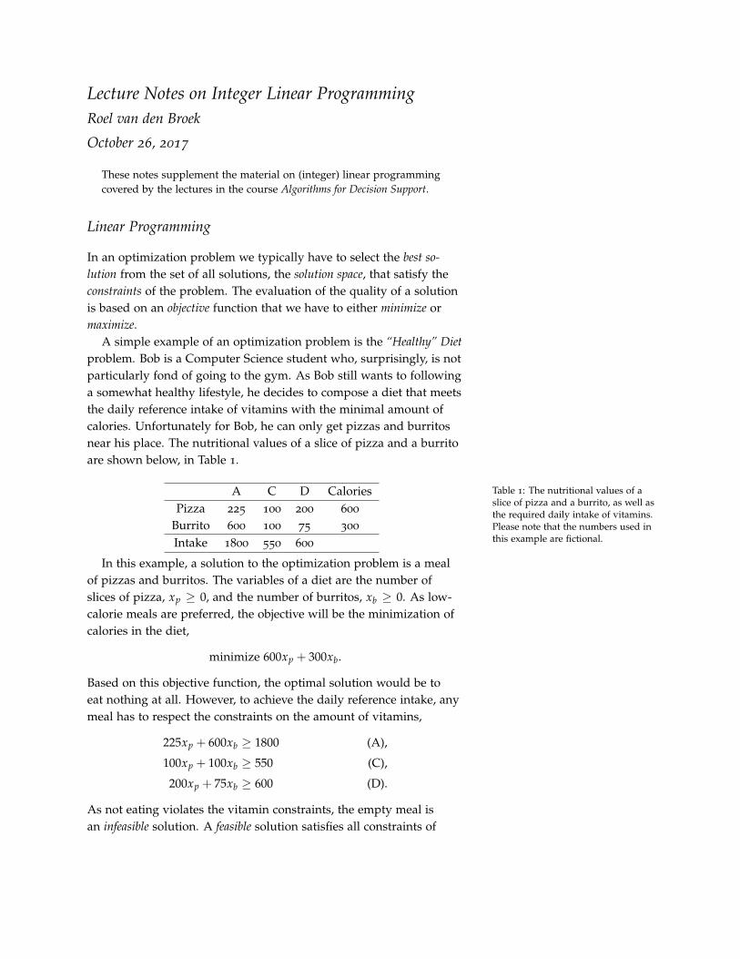
A simple example of an optimization problem is the “Healthy” Dietproblem. Bob is a Computer Science student who, surprisingly, is notparticularly fond of going to the gym. As Bob still wants to followinga somewhat healthy lifestyle, he decides to compose a diet that meetsthe daily reference intake of vitamins with the minimal amount ofcalories. Unfortunately for Bob, he can only get pizzas and burritosnear his place. The nutritional values of a slice of pizza and a burritoare shown below, in Table 1.

A C D CaloriesPizza 225 100 200 600

Burrito 600 100 75 300

Intake 1800 550 600

Table 1: The nutritional values of aslice of pizza and a burrito, as well asthe required daily intake of vitamins.Please note that the numbers used inthis example are fictional.

In this example, a solution to the optimization problem is a mealof pizzas and burritos. The variables of a diet are the number ofslices of pizza, xp ≥ 0, and the number of burritos, xb ≥ 0. As low-calorie meals are preferred, the objective will be the minimization ofcalories in the diet,

minimize 600xp + 300xb.

Based on this objective function, the optimal solution would be toeat nothing at all. However, to achieve the daily reference intake, anymeal has to respect the constraints on the amount of vitamins,

225xp + 600xb ≥ 1800 (A),

100xp + 100xb ≥ 550 (C),

200xp + 75xb ≥ 600 (D).

As not eating violates the vitamin constraints, the empty meal isan infeasible solution. A feasible solution satisfies all constraints of

http://www.cs.uu.nl/docs/vakken/mads/

lecture notes on integer linear programming 2

the optimization problem. Figure 1 shows the constraints as wellas the area containing feasible solutions, called the feasible region1.

1 The feasible region is empty if nosolution satisfies all constraints, inwhich case the optimization problemitself is infeasible.

Furthermore, we can see in Figure 1 that the optimal meal2 consists2 Disclaimer you should not take this“optimal” solution as sound dietaryadvise. Any reliance you place on thesediets is strictly at your own risk.

of eating four burritos and one and a half slices of pizza each day, fora total of 2100 calories.

obje

ctiv

e

600x

p+

300x

b

8100

0

xb

xp

0 1 2 3 4 5 6 7 8 9

0

1

2

3

4

5

6

7

8

9

225xp + 600xb ≥ 1800

100xp + 100xb ≥ 550

200xp + 75xb ≥ 600

Figure 1: The colored area contains thefeasible solution to the “Healthy” Dietproblem. The gradient shows the valueof the objective function in the solutionspace.

The formulation of the “Healthy” Diet problem is an example ofLinear Programmaing (LP), also known as Linear Optimization. In linearprogramming, a solution is represented of one or more variables,which are called decision variables, and the domain of each variableis an interval on the real line. Furthermore, both the objective and theconstraints are linear3 in the variables.

3 The linearity property of linear pro-grams means that, with two variablesx and y, the objective and constraintscan contain expressions such as x + yand y− x, but, for example, not x

y , x2

or x · y, as the latter three are non-linearexpressions.

The general linear programming formulation of a minimization4

4 Maximizing the objective functionf (x) is equivalent to minimizing − f (x).


problem is

minimizen

∑i=1

cixi

subject ton

∑i=1

ai1xi ≤ b1

...n

∑i=1

aimxi ≤ bm

xi ≥ 0 ∀i ∈ {1, . . . , n} (domain),

(1)

where solutions are encoded by n decision variables, x1 to xn, withassociated costs c1 to cn, and the objective is to minimize the totalcost. The decision variables are subject to m constraints of the form5

5 Linear constraints such as ∑ aixi = bor ∑ aixi ≥ b can be rewritten to thisform as well. Strict inequalities suchas ∑ aixi < b are — usually — notallowed in a linear program, since theoptimal solution to the LP might not bewell-defined. For example, in the singlevariable LP

max x

s.t. x < 1

x ≥ 0,

no solution is maximal.

∑ni=1 aijxi ≤ bj, and n domain constraints, xi ≥ 0. An optimal solution

is any solution that satisfies the constraints and has minimal cost6.

6 An optimization problem is calledunbounded it is feasible and we can findan arbitrarily good feasible solution,i.e. the constraints in the problem donot produce an upper bound on thegoodness of feasible solutions.

For many applications, it is easier to use the matrix form of anLP instead of the sum formulation shown in (1). Denote vectorsx = (x1, . . . , xn), c = (c1, . . . , cn), b = (b1, . . . , bm) and let

A =

a1,1 a1,2 · · · a1,n

a2,1 a2,2 · · · a2,n...

.... . .

...am,1 am,2 · · · am,n

.

Then the linear program (1) can be written in matrix form7 as7 The notation x ≥ 0 indicates that allelements xi of x should be at least zero.minimize cTx

subject to

Ax ≤ b

x ≥ 0.

(2)

Techniques to find the optimal solution of a linear program isnot covered in the lecture notes. Examples are shown on the lectureslides and in the first two chapters of Chvatal8. 8 Vasek Chvatal. Linear Programming.

Macmillan, 1983

Modeling

Linear programming is a flexible technique that can be applied tomany real-world problems. A major advantage of modeling a prob-lem as an LP is that linear programs are efficiently solvable. Thatis, the computation time of an LP is polynomial9 in the number of 9 In complexity theory we would denote

this property as LP ∈ P . More on thisin a few lectures.


variables and constraints. With the current state-of-the-art of com-mercial and open-source solvers, it is rarely necessary or beneficialto implement your own custom solver. The major challenge of linearprogramming is in the problem modeling: how do we translate anoptimization problem to a linear program that can be processed ef-ficiently by a solver? What decision variables will we use to encodethe solutions of the problem, and how can we rewrite the problemconstraints to linear equations? To further complicate matters, thereare problems for which we cannot formulate linear programs10. As 10 Fortunately, extensions to linear pro-

gramming allow us to model a muchbroader class of optimization problems,albeit at the cost of computation time insolvers.

there are no algorithms available that decide how, and if, an opti-mization problem can be modeled as an LP, modeling often has to bedone manually. In the next sections, we will look at several examplesof optimization problems, and show you how they can be modeled aslinear programs.

Assignment Problem

In the Assignment problem, we have n jobs that need to be per-formed; each job takes T time to complete. As we obviously do notwant to do the work ourselves, we hire n workers to perform thejobs. Each worker can be hired for at most T time units. The cost ofhiring a certain worker depends on both the employment durationand the job he/she has to perform; if worker i spends a fraction a ofits time on job j, it will cost us a times Cij. The objective of the As-signment problem is to assign the workers to jobs such that all jobsare completed with the lowest total cost.

To model this problem as a linear program, we need to have de-cision variables that encode all possible solutions, i.e. the differentassignments. A solution to the Assignment problem should statefor each worker the time11 it spends on each job. As the processing 11 Note that the problem description

does not limit a worker to a single job;workers can switch between jobs.

time of a job equals the maximum hiring duration of a worker, thisis equivalent to stating the fraction of job j completed by worker i.Therefore, we introduce for each worker-job pair (i, j) the variablexij ∈ [0, 1] that indicates the fraction of job j that is performed byworker i. The objective then becomes the minimization of the sum ofall variables xij multiplied by their cost Cij.

To ensure that each job j is completed, we have the constraintthat the sum of the fraction of work spend by all workers on job jis precisely one. Similarly, the work load of each worker i, the totalfraction of their time allocated to all jobs, should be no more thanone. The LP formulation of this model is shown below, (3).


minn

∑i=1

n

∑j=1

Cijxij (3a)

s.t.n

∑i=1

xij ≤ 1 ∀j ∈ {1, . . . , n} (work load) (3b)

n

∑j=1

xij = 1 ∀i ∈ {1, . . . , n} (job completion) (3c)

xij ∈ [0, 1] ∀i, j ∈ {1, . . . , n} (domain) (3d)

In the current problem statement, workers are allowed to be as-signed to multiple jobs, the only requirement is that they should notperform more than a single jobs worth of work. In practice, it mightbe inefficient if a worker has to switch jobs. Therefore, the constraintthat each job is completed by a single worker is preferable. That is,worker i performs job j either entirely or not at all. To model thisconstraint we restrict the domain of the xij variables, constraint (3d),to binary values,

xij ∈ {0, 1} ∀i, j ∈ {1, . . . , n} (binary domain). (3d′)

The meaning of the variables stays the same,

xij =

1 if worker i performs job j,

0 otherwise.

Integer Linear Programming

The program described by (3) with the additional constraints (3d′) isan example of Integer Linear Programming, abbreviated as ILP or IP,where each variable is restricted to integer values12. Integer linear 12 Models that contain both integer

and continuous variables are knownin literature as Mixed Integer (Linear)Programs or MI(L)Ps.

programming is an important tool in combinatorial optimization,as many problems feature discrete decisions that can be modeled inan ILP. We will examine a few examples of such problems in theselecture notes.

In our first example of an LP, the “Healty” Diet problem, supposethat Bob wants to avoid meals that consist of partial burritos or pizzaslices, as he does not like to eat leftovers of the previous day. Similarto the Assignment problem, Bob only has to set the domain of thevariables, xp and xb, to integers in his model to get the desired result:


min 600xp + 300xb (4a)

s.t.

225xp + 600xb ≥ 1800 (A) (4b)

100xp + 100xb ≥ 550 (C) (4c)

200xp + 75xb ≥ 600 (D) (4d)

xp, xb ∈N0 (domain) (4e)

Figure 2 shows the resulting feasible region of the new integerlinear program. Note that each feasible solution to the ILP is alsofeasible in the original LP, but not vice versa. In the ILP formulation,we now have three optimal solutions (x∗p, x∗b ), namely (2, 4), (1, 6)and (0, 8), each worth 2400 calories.

obje

ctiv

e

600x

p+

300x

b

8100

0

xb

xp

0 1 2 3 4 5 6 7 8 9

0

1

2

3

4

5

6

7

8

9

Figure 2: The colored dots are thefeasible solution of the “Healthy” Dietproblem without partial meals, thecolor of each dot shows the objectivevalue.

Knapsack

In the classical Knapsack problem we have n valuable items, and wewant to maximize our profit by selling some of them. However, thecarrying capacity B of our knapsack is limited, so we have to decide


which items we will take with us. Item i has a value of ci and weighsai units. Breaking items into smaller parts makes them worthless, sowe are not allowed to take a fractional part of an item.

A solution to the Knapsack problem consists of a set of items. Wecan encode the solutions by introducing a variable xi for every item i,indicating whether we take the item or not,

xi =

1 if we put item i in the knapsack,

0 otherwise.

These variables are binary, hence we are creating an integer linearprogram. Since an optimal solution should maximize the total profitof the selected items, and the main constraint of the problem is thecapacity of knapsack, we can use the ILP model

maxn

∑i=1

cixi

s.t.n

∑i=1

aixi ≤ B (capacity)

xi ∈ {0, 1} ∀i ∈ {1, . . . , n}.

(5)

Maximum Independent Set Problem

An example of an optimization problem on graphs is the Maximum

Independent Set problem. An independent set of a graph G =

(V, E) is a subset of vertices S ⊆ V with the property that no twovertices in S are adjacent in graph G. The Maximum Independent Setproblem consists of finding a largest independent set in the graph.

Figure 3: The colored vertices forman independent set of the graph, asno neighboring vertices are colored.Since this graph does not admit a largerindependent set, the colored vertices area maximum independent set.

Similar to the Knapsack problem, a natural solution represen-tation is to associate a binary variable to each vertex in the graph,modeling the decision on whether the vertex is included in the in-dependent set or not. Suppose that graph G has n vertices, v1 to vn.Then we associate a binary variable xi to each vertex, such that

xi =

1 if vi is in the independent set,

0 otherwise.

With this choice of variables, the objective simply becomes themaximization of the sum of all n variables. To define the constraints,we can observe that at most one vertex of each pair of neighboringvertices in the graph can be included in the independent set. Thisresults in the following integer linear program,


maxn

∑i=1

xi (6a)

s.t.

xi + xj ≤ 1 ∀(vi, vj) ∈ E (non-adjacent) (6b)

xi ∈ {0, 1} ∀vi ∈ V (domain). (6c)

Although modeling the Maximum Independent Set problemas an ILP is rather straightforward, finding the largest independentset is still a difficult task. In contrast to linear programs, which are allsolvable to optimality in polynomial time (in the number of variablesand constraints), there is no polynomial bound on the computationtime known for many integer linear programs13. 13 For the Maximum Independent

Set problem, it is unlikely that such abound exists, as it is a known NP-hardproblem. For more information, see thelectures on complexity theory.

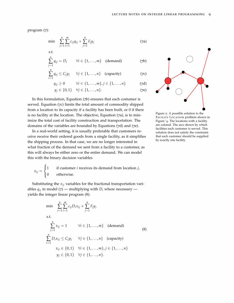
Facility Location Problem

Another classical example in combinatorial optimization is the Ca-pacitated Facility Location problem. A manufacturing com-pany has to meet the demand of m customers, with the demandof customer i ∈ {1, . . . , m} equal to Di ≥ 0. The company wantsto open a number of new production facilities, such that the costsof transporting the manufactured commodity to the customers isminimal. There are n possible building sites for the facilities, andthe cost of transporting of one unit of the commodity from locationj ∈ {1, . . . , n} to customer i is cij. Of course, constructing a facilitycosts money as well, the fixed construction cost at location j being Fj.Furthermore, the production capacity at location j is limited to Cj.

Figure 4: In the Facility Location

problem, there are n locations, shownin as circles, available for the facili-ties. These facilities have to serve mcustomers, the black dots.

In this problem we have to make two types of decisions:

• where to open the facilities, and

• how customers obtain their goods.

In line with this distinction, we define two types of variables forlocation j ∈ {1, . . . , n} and customer i ∈ {1, . . . , m}, namely thelocation variable

yj =

1 if we open a facility at location j

0 otherwise,

and the transportation variable

qij = the quantity of goods transported from location j to i.

One way of modeling the problem is the mixed integer linear


program (7):

minn

∑j=1

m

∑i=1

cijqij +n

∑j=1

Fjyj (7a)

s.t.n

∑j=1

qij = Di ∀i ∈ {1, . . . , m} (demand) (7b)

n

∑i=1

qij ≤ Cjyj ∀j ∈ {1, . . . , n} (capacity) (7c)

qij ≥ 0 ∀i ∈ {1, . . . , m}, j ∈ {1, . . . , n} (7d)

yj ∈ {0, 1} ∀j ∈ {1, . . . , n}. (7e)

Figure 5: A possible solution to theFacility Location problem shown inFigure ‘4. The locations with a facilityare colored. The arcs shown by whichfacilities each customer is served. Thissolution does not satisfy the constraintthat each customer should be suppliedby exactly one facility.

In this formulation, Equation (7b) ensures that each costumer isserved. Equation (7c) limits the total amount of commodity shippedfrom a location to its capacity if a facility has been built, or 0 if thereis no facility at the location. The objective, Equation (7a), is to min-imize the total cost of facility construction and transportation. Thedomains of the variables are bounded by Equations (7d) and (7e).

In a real-world setting, it is usually preferable that customers re-ceive receive their ordered goods from a single facility, as it simplifiesthe shipping process. In that case, we are no longer interested inwhat fraction of the demand we sent from a facility to a customer, asthis will always be either zero or the entire demand. We can modelthis with the binary decision variables

xij =

1 if customer i receives its demand from location j,

0 otherwise.

Substituting the xij variables for the fractional transportation vari-ables qij in model (7) — multiplying with Di where necessary —yields the integer linear program (8):

minn

∑j=1

m

∑i=1

cijDixij +n

∑j=1

Fjyj

s.t.n

∑j=1

xij = 1 ∀i ∈ {1, . . . , m} (demand)

n

∑i=1

Dixij ≤ Cjyj ∀j ∈ {1, . . . , n} (capacity)

xij ∈ {0, 1} ∀i ∈ {1, . . . , m}, j ∈ {1, . . . , n}yj ∈ {0, 1} ∀j ∈ {1, . . . , n}.

(8)


Towards solving an ILP: LP-relaxation

In our example of the “Healty” Diet problem, we restricted the do-main of the decision variables to integer values to find a meal with-out leftovers. The solution space of the resulting integer linear pro-gram was a subset of the set of feasible solutions of the original prob-lem, with the integral optimum containing slightly more calories thanthe best fractional solution. In general, restricting the domains ofthe variables will never lead to a better solution. The converse alsoholds: relaxing the domain of a variable from integers to a contin-uous real interval — that encompasses the original integral values— never results in a worse optimum. The linear program obtainedby relaxing the integrality constraints of an ILP is known as the LP-relaxation of the original problem. As linear programs can be solvedmore efficiently than integer linear programs, LP-relaxations providean efficient procedure to find a bound14 on the optimum of an ILP: 14 The LP-relaxation provides a lower

bound on the optimal objective valuefor minimization problems, and anupper bound in case of maximization.

1. Relax the integrality constraints.

2. Solve the resulting linear program.The LP-relaxation of the integer linear

program

min cT x

s.t.

Ax ≤ b

x ∈N0

is the linear program

min cT x

s.t.

Ax ≤ b

x ≥ 0.

If the optimal solution to the LP-relaxation happens to be inte-gral, then you do not even have to solve the ILP itself, because thebound guarantees that it will not find a better solution. Even if theLP-relaxation has a fractional optimal solution, the bound it providesis crucial in solving the ILP, as we will see in a few sections.

In the example of the Capacitated Facility Location prob-lem, we have seen that there can be multiple models of the sameproblem, and the optimal objective value of these models should bethe same. However, the LP-relaxations of the different models do nothave not result in the same bound on the optimum, as their solutionsspaces can be different. Due to the importance of the LP-relaxationbounds, we usually want to find a model with strong bound on theILP. In the next sections, we will see some examples of problems withmultiple models, for which we can prove that the LP-relaxation ofone model gives a better bound than the other.

Facility Location Problem (Revisited)

A common variant of the Facility Location problem is to removethe capacity constraints of the facilities, i.e. each facility can produceenough to supply all customers. Furthermore, in this Uncapaci-tated Facility Location problem we require each customer tobe served by exactly one facility. We can model this problem witha small modification to the ILP formulation shown in Equation (8).The capacity constraint is no longer needed. However, we do have to


ensure that customer i is only served from location j if we selected jas the construction site for a facility. Using the notation dij = cijDi,we get the ILP formulation

minn

∑j=1

m

∑i=1

dijxij +n

∑j=1

Fjyj (9a)

s.t.n

∑j=1

xij = 1 ∀i ∈ {1, . . . , m} (9b)

xij ≤ yj ∀i ∈ {1, . . . , m}, j ∈ {1, . . . , n} (9c)

xij ∈ {0, 1} ∀i ∈ {1, . . . , m}, j ∈ {1, . . . , n} (9d)

yj ∈ {0, 1} ∀j ∈ {1, . . . , n}. (9e)

Equation (9c) creates nm constraints, one for each of transportationvariable, to prevent customers being served by non-existing facilities.We can construct a more compact model by observing that if alltransportation variables x1j to xmj of location j are at most yj, thenthe sum of the variables xij will not be more than myj. Therefore,we can combine the nm separate transportation constraints into naggregated transportation constraints per location:

minn

∑j=1

m

∑i=1

dijxij +n

∑j=1

Fjyj (10a)

s.t.n

∑j=1

xij = 1 ∀i ∈ {1, . . . , m} (10b)

m

∑i=1

xij ≤ myj ∀j ∈ {1, . . . , n} (10c)

xij ∈ {0, 1} ∀i ∈ {1, . . . , m}, j ∈ {1, . . . , n} (10d)

yj ∈ {0, 1} ∀j ∈ {1, . . . , n}. (10e)

Both the separated model, (9), and the aggregated model, (10),have the same optimal value, yet the latter ILP has fewer constraints,suggesting that the compact formulation might be the preferredmodel for this problem. However, a comparison of the LP-relaxationsof both models — obtained by replacing the domain constraints inthe ILPS with 0 ≤ xij ≤ 1 and 0 ≤ yj ≤ 1 — will show that theseparated model provides a stronger bound on the optimal solutionof the ILP.

Theorem 1. The lower bound on the optimum value of the Uncapac-itated Facility Location problem obtained from the LP-relaxation


of separated model, Equation (9), is at least as high as the bound of the LP-relaxation of the aggregated model, Equation (10).

Proof. Let PILP, PLPS and PLPA be the sets of feasible solutions of re-spectively the ILP model15, the LP-relaxation of the separated model 15 The solution space and optimal value

of models (9) and (10) is the same.(9) and the LP-relaxation of the aggregated model (10). Every feasi-ble solution to the ILP is feasible for the two LP-relaxations as well,hence

PILP ⊆ PLPS and

PILP ⊆ PLPA.

Recall our earlier observation that, for any j ∈ {1, . . . , n},

∀i ∈ {1, . . . , m} : xij ≤ yj =⇒m

∑i=1

xij ≤ myj.

Since the two models differ only in constraints (9c) respectively (10c),each solution in PLPS is also a feasible solution to the aggregatedmodel:

PLPS ⊆ PLPA.

L1

y1 = 12

L2

y2 = 12

C1

C2

x11 = 1

x22 = 1

x12 = x21 = 0

Figure 6: A fractional solution to theUncapacitated Facility Location

problem with two locations and twocustomers.

In contrast, not all feasible solutions to the LP-relaxation of theaggregated model satisfy the constraints in (9c). Let’s consider thefollowing example of two customers, c1 and c2, and two locations,l1 and l2. A possible solution to this problem is y1 = y2 = 1/2,x11 = x22 = 1 and x12 = x21 = 0, as is shown in Figure 6. Eachcustomer is fully served in this solution and, since

x11 + x21 = 1 + 0 ≤ 2 ∗ 12= 2 ∗ y1 and

x12 + x22 = 1 + 0 ≤ 2 ∗ 12= 2 ∗ y2,

this solution is feasible for the LP-relaxation of the aggregated modelin Equation (10). However, the solution is not in PLPS, as it does notsatisfy all constraints in the LP-relaxation of the separated model:

x11 = 1 >12= y1.

Therefore, we have the following relation on the feasible solution sets:

PILP ⊆ PLPS ⊆ PLPA.

Let the optimal values of the three solution sets be ZILP, ZLPS andZLPA, then the relation above implies that

ZILP ≤ ZLPS ≤ ZLPA,

showing that the bound of the LP-relaxation of the separated modelis at least as good as the bound obtained from the aggregated modelof the Uncapacitated Facility Location problem.


Minimum Spanning Tree

A common task when working on graphs is to find a minimum span-ning tree. A tree T of a connected, undirected graph G = (V, E) is asubset of the edges E that is both connected and without cycles. TreeT is a spanning tree if it connects all n vertices V in G. Let ce be thecost of including edge e ∈ E in the spanning tree, then a minimumspanning tree is a spanning tree of minimum total cost of the includededges. An example is shown in Figure 7.

A B

C

D

E

1

1 1

0

0

0

Figure 7: An undirected graph withedge costs. The edges of a minimumspanning tree are colored.

Minimum spanning trees are usually constructed with an opti-mal, greedy algorithm, as it is much more efficient than known ILPmodels. Nevertheless, formulating the Minimum Spanning Tree

problem as an integer linear program allows us to look at some use-ful modeling patterns and provides another opportunity to compareLP-relaxations.

We will formulate two different models of the Minimum Span-ning Tree problem in this section. Both models use the same binaryvariables, one for each edge e ∈ E in the graph:

xe =

1 if e is included in the spanning tree,

0 otherwise.

We use two basic properties of a spanning tree T to create the firstmodel:

1. |T| = |V| − 1, i.e. the size of the tree is precisely one less than thenumber of vertices in the graph16. 16 The proof of this property is left as an

exercise to the reader. Have fun.2. T has no cycles.

The first property can be formulated directly as a constraint. Tomodel the second property, we use the (equivalent) property thatany subset S ⊂ V connected by |S| or more edges contains a cycle.Let

E(S) = {e = (v, w) ∈ E | v, w ∈ S},

be the set of edges between vertices in S ⊂ V, then the spanningtree T has no cycle in the set of vertices S if the sum of all xe withe ∈ E(S) is at most |S| − 1. This type of constraint is known as asubtour elimination constraint. To ensure that the entire spanning treedoes not contain a cycle, we have to add such a constraint for everysubset S of V, as can be seen in the first ILP model in Equation (11),


min ∑e∈E

cexe (11a)

s.t.

∑e∈E

xe = |V| − 1 (11b)

∑e∈E(S)

xe ≤ |S| − 1 ∀S ⊂ V (subtour) (11c)

xe ∈ {0, 1} ∀e ∈ E. (11d)

Our second model does not translate the acyclicity property di-rectly to a set of constraints. Instead of subtour elimination, it usesthe property that in any partition (S, V \ S)17 of the graph G = (V, E) 17 A partition (S, V \ S) of a graph G =

(V, E) splits the graph into two sets,S ⊆ V and V \ S, removing all edgesthat do not connect a vertex in S to avertex in V \ S. That is, the partition(S, V \ S) is the graph G′ = (V, E′) with

E′ = {e = (v, w) ∈ E | v ∈ S, w ∈ V \ S}.

the spanning tree has at least one edge from S to V \ S. Let the cut setδ(S) of S ⊂ V be the set of edges connecting S to V \ S,

δ(S) = {e = (v, w) ∈ E | v ∈ S, w ∈ V \ S},

then the cut set model is

min ∑e∈E

cexe (12a)

s.t.

∑e∈E

xe = |V| − 1 (12b)

∑e∈δ(S)

xe ≥ 1 ∀S ⊂ V (cut set) (12c)

xe ∈ {0, 1} ∀e ∈ E. (12d)

Unfortunately, the number of constraints in the two models growsexponentially with the size of the graph due to Equation (11b)and (12c). Although this makes both models impractical for largegraphs, we can prove that the LP-relaxation of the subtour modelgives a stronger lower bound on the optimum.

Theorem 2. The lower bound on the optimal value of the Minimum

Spanning Tree problem obtained from the LP-relaxation of the subtourmodel, Equation (11), is as least as high as the bound of the LP-relaxation ofthe cut set model, Equation (12) .

Proof. Let PLPS and PLPC be the feasible regions of the LP-relaxationsof respectively the subtour model and the cut set model. We startby showing that each feasible solution to relaxed subtour model isfeasible for the relaxed cut set models as well.

First note that, for any subset S of V, we have that

E(S) ∪ δ(S) ∪ E(V \ S) = E, (13)


as each edge e ∈ E connects either two vertices in S, two vertices inV \ S or a vertex in S to a vertex in V \ S.

Let x = {xe | e ∈ E} ∈ PLPS, i.e. a feasible solution to the LP-relaxation of the subtour model, then for any vertex set S ⊂ V

|V| − 1 = ∑e∈E

xe by Equation (11b)

= ∑e∈E(S)

xe + ∑e∈δ(S)

xe + ∑e∈E(V\S)

xe by Equation (13)

≤ |S| − 1 + ∑e∈δ(S)

xe + |V| − |S| − 1 by Equation (11c)

= |V| − 2 + ∑e∈δ(S)

xe,

which we can rewrite to

∑e∈δ(S)

xe ≥ 1. (14)

A B

C

D

E

1/2

1/2 1/2

1

1/2

1

Figure 8: A fractional, feasible solutionto the LP-relaxation of the cut setmodel, Equation (12), with the values ofvariables xe on the edges. The total costof this solution is 3/2. The colored edgesdo not satisfy the subtour constraint inEquation (11c).

As this holds for every subset of vertices in V, any feasible solu-tion to the LP-relaxation of model (11) satisfies the cut set constraintsin Equation (12c); hence, x belongs to PLPC, the feasible region of theLP-relaxation of the cut set model.

The example in Figure 8 shows that converse does not hold,as some solutions in PLPC are not feasible with respect to the LP-relaxation of the subtour model. We conclude that

PLPS ⊂ PLPC,

and, analogue to the proof of Theorem 1, that the lower bound ofsubtour model is at least as good as the lower bound of the cut setmodel.

Modeling the Minimum Spanning Tree problem as an ILPmight seem like a pointless exercise, as both models contain an ex-ponential number of constraints, and faster algorithms are availablefor this problem. However, the two constraint types shown in thissection are applicable to other, more difficult problems as well. Forexample, a solution to the classical Travelling Sales Person

problem, where we have to find a shortest tour that visits all verticesin a graph, should not contain any cycles smaller than the number ofvertices in the graph. An ILP model with subtour constraints is muchmore interesting18 for such a computationally hard problem, than it

18 We still have the “minor” problemof the exponential number of subtourconstraints. However, it turns outthat, in practice, you rarely need allof them to find a solution withoutsubtours. A common strategy is to startwithout (many) subtour constraints,and iteratively solve the model, addingnew constraints for any subtours inthe resulting solution, until a solutionwithout subtours is found.

is for the Minimum Spanning Tree problem.

Solving an ILP: branch-and-bound

We have seen examples of modeling optimization problems as integerlinear programs, and showed that we can get a bound on the optimal


objective value by relaxing the integrality constraints. However, thisdoes not provide us with an algorithm to actually solve the ILP mod-els. We might be fortunate enough to obtain an integral solution fromthe LP-relaxation, but this will not happen for all problem types andinstances.

The standard framework used to solve an ILP is branch-and-bound,where we repeatedly divide the problem in smaller subproblems.This framework creates a tree structure, with at the root the orig-inal problem. Each parent node in the tree splits, or branches, intomultiple child nodes by creating copies of the parent problem withadditional constraints, such that the child solution spaces partitionthe parent solution space.

If we would only branch, then the leaves of the tree would cor-respond to subproblems that either are infeasible or have all theirvariables fixed. By constructing the entire tree, we enumerate all fea-sible solutions to the original problem, and are thus guaranteed tofind the optimum. However, as the size of the tree tends to grow ex-ponentially with the number of variables in the model, it will take along time to actually find the optimal solution.

To avoid complete enumeration of solution space, we bring thebounding part of branch-and-bound into play. It uses the LP-relaxationof the integer linear program of the problem at each node to ob-tain a lower bound — in case of a minimization problem19 — and 19 In a maximization problem, the LP-

relaxation gives the upper bound andthe construction heuristic the lowerbound.

a heuristic that produces an upper bound on the optimal value byconstructing a good, integral solution20. Instead of simply branching

20 Many heuristics can be used to findfeasible, but not necessarily optimal,solutions to the ILP. A simple exampleis to round a fractional solution of theLP-relaxation to feasible integer values.

at each possible node, we use the bounds on the optimal value of thesubproblems to eliminate or bound unpromising branches early.

There are then four different outcomes at each node:

1. The subproblem of the branch is infeasible. In this case, we do notsplit the subproblem in smaller parts. This node becomes a leaf.

2. The solution of the LP-relaxation is integral. We have found theoptimal solution of this node, so further branching on this sub-problem will not result in a better solution. This node becomes aleaf. We update the best solution seen so far if necessary.

3. The lower bound on the current subproblem is at least as highas the objective value of the best solution found so far. Since wehave already discovered a solution that is better than the best thisbranch has to offer, we gain nothing by exploring it any further.This node becomes a leaf.

4. The lower bound on the current subproblem is lower than the ob-jective value of the best solution found so far. If we have a heuris-tic available, we will compute an upper bound on this subproblem,


and update the best solution seen so far if needed. We continuebranching on this node.

As this procedure only prunes unpromising branches, we geta tremendous speed up of the search process without losing theoptimal solution. However, branch-and-bound does not provideany guarantees on the computation time, and is heavily affected bythe implementation. As mentioned earlier, branch-and-bound is aframework, meaning that many parts have to be filled in by the user:

• Model Clearly, the model has a large influence on the search pro-cess. It determines the variables on which we can branch as wellas the bound of the LP-relaxation. The better the bound of the LP-relaxation, the more likely it is that we can eliminate bad branchesearly.

• Integer heuristic Similar to the LP-relaxation bound, a goodheuristic for integral solutions allows early pruning of unpromis-ing branches, reducing the solution space.

• Search strategy Since we are essentially constructing a tree nodeby node during branch-and-bound, we need to decide during thesearch, when the tree is not yet constructed fully, which node ofthe tree we wish to evaluate and branch on. Possible approachesare depth-first, breadth-first or selection strategies that expand themost “promising” node.

• Branching strategy In addition to selecting a node to branch on,we need to decide how we will branch. That is, how will we splitthe solution space of the selected node. A common approach whenbranching on decision variables is to split its domain into twoparts. For example, if we have a binary decision variable xi ∈{0, 1}, we can branch into xi = 0 and xi = 1. In case of an integraldecision variable xj ≥ 0, we might create two21 branches, splitting 21 Similar to a binary decision variable,

if an integral decision variable has anupper bound of k, with k not too large,we branch into k child nodes, one foreach possible value of the variable.

the domain in 0 ≤ xj ≤ 4 and xj ≥ 5. If the subproblem containsmore than one decision variable on which we can branch, we needto select one of them. For example, a simple strategy for decisionvariables is to select the variable with the most fractional22 value. 22 The rationale behind this strategy is

that fixing a highly fractional — closeto 1/2 — binary variable is likely to havea big impact on the overall solution,which hopefully allows us to prune thebranch with “wrong” decision early inthe search.

Branching on other aspects, such as xi + xj ≤ 6 and xi + xj ≥ 7,is possible as well, as long as at least one of the branches preservesthe optimal solution of the parent node in the branch-and-boundtree.

Knapsack (Revisited)

To illustrate the branch-and-bound framework, let us consider thefollowing example of the Knapsack problem. Our knapsack has a


capacity B of 15, and we have five items that we could carry in thebackpack. The values ci and weights ai are shown in Table 2. Usingthese data as input for ILP formulation (5) of the Knapsack problemgives us model (15):

i 1 2 3 4 5ci 8 12 7 15 12ai 4 8 3 6 5

ci/ai 2 11/2 21/3 21/2 22/5

Table 2: The values ci , weights ai andvalue-to-weight ratios of the five itemsin Knapsack problem.

max 8x1 + 12x2 + 7x3 + 15x4 + 12x5

s.t. 4x1 + 8x2 + 3x3 + 6x4 + 5x5 ≤ 15

x1, x2, x3, x4, x5 ∈ {0, 1}.

(15)

To use the branch-and-bound framework, we need to specify thesearch and branching strategies. The simple breadth-first-search strat-egy is used to explore the branch-and-bound tree, evaluating thenodes level by level. We base our branching strategy on the intuitionthat items with a large value-to-weight ratio are more favorable toput in the knapsack than low value, high weight items in the Knap-sack problem. Therefore, it is likely that the exclusion of an itemwith a high value-to-weight ratio will lead to a bad solution, allowingus to cut off the corresponding branch in the tree early in the searchprocess. The branching strategy that exploits this idea is to branch onthe binary decision variables in non-increasing value-to-weight ratio:x5 → x4 → x3 → x1 → x2.

Lower bounds can be obtained at each node by rounding down thefractional part of the optimal solution23 to the LP-relaxation. Figure 9

23 An optimal solution to the LP-relaxation can be constructed efficientlyby greedily selecting items with thehighest value-to-weight ration until theknapsack is full.

shows the branch-and-bound tree of our example.The exploration order of the nodes of the branch-and bound tree is

shown below:

N0. The root node corresponding to the original ILP model shownin(15). The lower bound heuristic constructs an initial solution; theglobal lower bound becomes 34. We branch on decision variablex5.

N1. The upper bound on the optimal value of this node is less than thecurrent best solution. We eliminate this branch.

N2. The optimal solution to the LP-relaxation is equal to the solution atthe root. We branch on x4.

N3. The upper bound of this node is less than the current best solu-tion. We eliminate this branch.

N4. The optimal solution of the LP-relaxation is equal to the solution atthe root. We branch on x3.

N5. The optimal solution of the LP-relaxation is integral, and is betterthan the current best solution; the global lower bound becomes 35.As the solution to the LP-relaxation is optimal for the ILP as well,we do not branch on this node.


1/4, 0, 1, 1, 1

34 36N0

1, 1/4, 1, 1, 0

27 33N1

x5 = 0

1/4, 0, 1, 1, 1

34 36N2

1, 3/8, 1, 0, 1

30 311/2N3

x4 = 0

1/4, 0, 1, 1, 1

34 36N4

1, 0, 0, 1, 1

35 35N5

x3 = 0

1/4, 0, 1, 1, 1

34 36N6

0, 1/8, 1, 1, 1

34 351/2N7

0, 0, 1, 1, 1

34 34N9

x2 = 0

0, 1, 1, 1, 1

infeasibleN10

x2 = 1

x1 = 0

1, 0, 1, 1, 1

infeasibleN8

x1 = 1

x3 = 1

x4 = 1

x5 = 1

Figure 9: A branch-and-bound tree forthe instance of Knapsack shown inTable 2. Each node shows at the top anoptimal solution to the LP-relaxationof the subproblem, and at the bottomright the corresponding objective value.This is an upper bound on the optimalsolution to the ILP. A lower bound,obtained by rounding down fractionaldecision variables in the LP solution,can be found in the bottom left ofa node. The labels at the arcs showbranching choices. A lower bound isunderlined if it improves the currentbest lower bound. Bold values in thesolution indicate variables that are fixedby branching. The branch-and-boundtree shows that 35 is the optimal valueof this Knapsack instance.


N6. Th optimal solution of the LP-relaxation is equal to the solution atthe root. We branch on x1.

N7. We branch on x2.

N8. The node is infeasible, because the total weight of the fixed items,18, exceed the maximum capacity of the knapsack. We do notbranch on this node.

N9. The upper bound of this node is less than the current best solu-tion. We eliminate this branch.

N10. The node is infeasible, because the total weight of the fixed items,22, exceed the maximum capacity of the knapsack. We do notbranch on this node.

The optimal solution is then the best solution that we have seen overall nodes. In this case, the solution consists of items 1, 4 and 5, with atotal value of 35.

Valid Inequalities

Branch-and-bound relies heavily on a strong LP-relaxation bound onthe optimum of each node in the search tree. In previous sections wehave seen that modeling choices in the ILP affect the strength of thebound. However, a good model is not always sufficient to find theintegral optimum in reasonable time. In that case, we can strengthenthe LP-relaxation by introducing additional constraints, called validinequalities or cutting planes. These constraints cut off part of the LPsolution space to tighten the bound on the integral optimum, withoutremoving integral solutions. By preserving the ILP space, we ensurethat the strengthened model remains valid with regard to the originalinteger linear program. Enhancing branch-and-bound by adding thevalid inequalities at each node to cut off fractional solutions is knownas branch-and-cut.

Gomory’s cuts

Suppose that we have an integer linear program with decision vari-ables x1, . . . , xn ≥ 0, and a constraint of the form

∑i

aixi = b.

Then, for any integral solution that satisfies this constraint, the in-equality obtained by rounding down the constant and the coefficientsin the constraint,

∑ibaicxi ≤ bbc,


holds as well, since the decision variables are all non-negative. As theinequality does not cut off integral solutions, it is valid for the ILPmodel. This type of valid inequality is known as Gomory’s cut.

One of the advantages of Gomory cuts is that we can generatenew cutting planes efficiently from the final dictionary24 of the LP- 24

relaxation. Consider the following example ILP,

max 2x1 + x2

s.t.

x1 − x2 ≤ 1

2x1 + 2x2 ≤ 7

x1, x2 ∈N0,

(16)

depicted in Figure 10. obje

ctiv

e

2x1+

x 2

12

0x1

x2

0 1 2 3 4

0

1

2

3

4

x1 − x2 ≤ 1

2x1 + 2x2 ≤ 7

Figure 10: The feasible region of theLP-relaxation of model (16).

We turn an inequality constraints to an equality with a slack vari-able, modeling the gap between the left- and right-hand side of theoriginal inequality. Introducing slack variables x3 and x4 in ourmodel yields

max 2x1 + x2

s.t.

x1 − x2 + x3 = 1

2x1 + 2x2 + x4 = 7

x1, x2, x3, x4 ∈N0.

(17)

The optimal solution of the LP-relaxation of this model is x1 =

21/3, x2 = 11/4, x3 = x4 = 0, with a value of 53/4. In the dictio-nary of this solution, the non-zero decision variables x1 and x2 areexpressed in the other, zero-valued decision variables,

x1 = 214− 1

2x3 −

14

x4 (18)

x2 = 114+

12

x3 −14

x4. (19)

We can derive a Gomory cut from the constraint of any fractionaldecision variable. For example, as x2 = 1 1

4 , rewriting Equation (19) to

x2 −12

x3 +14

x4 = 114

,

and rounding down gives the Gomory cut

x2 − b12cx3 + b

14cx4 = x2 − x3 ≤ b1

14c = 1. (20)

Not only are Gomory cuts generated efficiently from the final dic-tionary of an LP-relaxation, these cutting planes are also effective. In


our example, the current optimal LP-relaxation solution does notsatisfy inequality (20), since

114− 0 > 1.

The property of cutting off the current optimal solution of the LP-relaxation holds for any Gomory cut generated from the constraintof a fraction decision variable. This property is a direct result of theexpressing the non-zero decision variable in terms of the zero-valueddecision variables:

xk = bk + ∑i:xi=0

aixi = bk > bbkc if xi is fractional.

Therefore, adding the valid inequality in Equation (20) as a con-straint to our example model model (17) and solving the LP-relaxationyields a new optimum of 51/2 at x1 = 2, x2 = 11/2, as is illustrated inFigure 11.

obje

ctiv

e

2x1+

x 2

12

0x1

x2

0 1 2 3 4

0

1

2

3

4Gomory cut

Figure 11: The feasible region of theLP-relaxation of model (16) with theGomory cut in Equation (20). The grayarea is removed by the Gomory cut.

Since the optimum of the LP-relaxation of the extended model isfractional as well, we can repeat the process of adding Gomory cutsand solving the resulting LP-relaxation, until an integral solutionis found. This procedure, the cutting plane algorithm, is guaranteedto converge to an integral solution, although the number of cuttingplanes added to the model can be exponential. In branch-and-cut,we do not necessarily have to continue until an integral solution isfound, as a good bound on the objective of a node in the search treeis sufficient in many cases.

Problem specific cuts

Although the previous valid inequalities are generally applicable,cutting planes that exploit the structure of a problem are often ableto strengthen the bound of an LP-relaxation much more efficiently.In this section we will look at two of these problem specific validinequalities.

1/2 1/2

1/2

1/2

1/2

Figure 12: The fractional solution to theMaximum Independent Set problemthat assigns 1/2 to each vertex in theodd cycle is optimal, with a value of21/2, but does not satisfy the odd cycleinequality.

The first example relates to the Maximum Independent Set

problem. It is based on the observation that at most half of the ver-tices in a cycle in a graph can be included in an independent set. Thisresults for model (6) in the valid inequality

∑i∈C

xi ≤|C| − 1

2,

where C ⊆ V is an odd cycle in the graph. The odd cycle25 inequality 25 Of course, a similar inequality existsfor even cycles as well. However, asfeasible fractional solution satisfythe even cycle inequality, we do notstrengthen the LP-relaxation bound byadding it to our model.

eliminates fractional solutions such as the one shown in Figure 12.Another type of problem specific valid inequalities can be derived

for the Knapsack problem. Suppose that we have a subset of items


I ⊂ {1, . . . , n} with a total weight larger than the capacity of ourknapsack. Then we know that we cannot carry all items in the subsetwith us, i.e. every feasible solution in model (5) should satisfy

∑i∈I

xi ≤ |I| − 1.

This type of cutting plane, known as a cover inequality, is applicableto many other problems as well, and is commonly used strategy inmodern solvers to tighten the bound of the LP-relaxation. As anexample of its usage, take the subset of items I = {1, 3, 4, 5} for theproblem instance listed in Table 2. Since

∑i∈I

ai = 4 + 3 + 6 + 5 > 15,

the set I covers our knapsack. The corresponding cover inequality

x1 + x3 + x4 + x5 ≤ 3

cuts off the optimal solution to the LP-relaxation, x3 = x4 = x5 = 1,x1 = 1/4.

References

Vasek Chvatal. Linear Programming. Macmillan, 1983.

lecture notes on integer linear · pdf filelecture notes on integer linear programming ......

Documents