lecture notes on electrodynamics phy 841 – … · lecture notes on electrodynamics phy 841 –...
TRANSCRIPT

LECTURE NOTES ON ELECTRODYNAMICSPHY 841 – 2017
Scott PrattDepartment of Physics and Astronomy
Michigan State University
These notes are for the one-semester graduate level electrodynamics course taught at Michi-gan State University. These notes are more terse than a text book, they do cover all the mate-rial used in PHY 841. They are NOT meant to serve as a replacement for a text. The coursemakes use of two textbooks: The Classical Theory of Fields by L.D. Landau and E.M. Lifshitz,and Classical Electrodynamics by J.D. Jackson. Anybody is welcome to use the notes to theirheart’s content, though the text should be treated with the usual academic respect when itcomes to copying material. If anyone is interested in the LATEX source files, they should con-tact me ([email protected]). Solutions to the end-of-chapter problems are also provided on thecourse web site (http://www.pa.msu.edu/courses/phy841). Please beware that this is a webmanuscript, and is thus alive and subject to change at any time.

PHY 841 CONTENTS
Contents
1 Special Relativity Primer 41.1 γ Factors and Such . . . . . . . . . . . . . . . . . . . . . . . . . . . . . . . . . . 4
1.2 Lorentz Transformations . . . . . . . . . . . . . . . . . . . . . . . . . . . . . . . 6
1.3 Invariants and the metric tensor gαβ . . . . . . . . . . . . . . . . . . . . . . . . 9
1.4 Four-Velocities and Momenta . . . . . . . . . . . . . . . . . . . . . . . . . . . . 9
1.5 Examples of Invariants . . . . . . . . . . . . . . . . . . . . . . . . . . . . . . . . 11
1.6 Tensors . . . . . . . . . . . . . . . . . . . . . . . . . . . . . . . . . . . . . . . . 13
1.7 Homework Problems . . . . . . . . . . . . . . . . . . . . . . . . . . . . . . . . 14
2 Dynamics of Relativistic Point Particles 162.1 Lagrangian for a Free Relativistic Particle . . . . . . . . . . . . . . . . . . . . . . 16
2.2 Interaction of a Charged Particle with an External Electromagnetic Field . . . . . 19
2.3 Motion in a Constant Magnetic Field . . . . . . . . . . . . . . . . . . . . . . . . 20
2.4 Gauge Transformations . . . . . . . . . . . . . . . . . . . . . . . . . . . . . . . 21
2.5 The Electromagnetic Field Tensor . . . . . . . . . . . . . . . . . . . . . . . . . . 21
2.6 Homework Problems . . . . . . . . . . . . . . . . . . . . . . . . . . . . . . . . 22
3 Dynamic Electromagnetic Fields 243.1 Lagrangian (Density) for Free Fields: Deriving Maxwell’s Equations . . . . . . . . 24
3.2 Pseudo-Vectors and Pseudo-Scalars . . . . . . . . . . . . . . . . . . . . . . . . . 27
3.3 The Stress-Energy Tensor of the Electromagnetic Field . . . . . . . . . . . . . . . 28
3.4 Hyper-Surfaces and Conservation of Energy, Momentum and Angular Momentum 32
3.5 Homework Problems . . . . . . . . . . . . . . . . . . . . . . . . . . . . . . . . 34
4 Electrostatics 364.1 Gauss’s Law . . . . . . . . . . . . . . . . . . . . . . . . . . . . . . . . . . . . . 36
4.2 Potential Energy of a Fixed Continuous Charge Distribution . . . . . . . . . . . . 36
4.3 Laplace’s Equations and a Fixed Point Charge . . . . . . . . . . . . . . . . . . . 37
4.4 Laplace’s Equations in Cartesian Coordinates . . . . . . . . . . . . . . . . . . . . 38
4.5 Laplace’s Equations and Solutions in Spherical Coordinates . . . . . . . . . . . . 38
4.6 Solutions to Laplace’s Equations in Cylindrical Coordinates . . . . . . . . . . . . 42
4.7 Boundary Value Problems . . . . . . . . . . . . . . . . . . . . . . . . . . . . . . 43
4.7.1 Method of Images . . . . . . . . . . . . . . . . . . . . . . . . . . . . . . 43
4.7.2 Boundary Value Problems Using Cartesian Solutions to the Laplace Equation 44
4.7.3 Boundary Value Problems Using Spherical Harmonics . . . . . . . . . . . 45
1

PHY 841 CONTENTS
4.7.4 Boundary Value Problems Using Cylindrical Harmonics . . . . . . . . . . 46
4.8 Solving Boundary Value Problems Numerically . . . . . . . . . . . . . . . . . . 47
4.9 Homework Problems . . . . . . . . . . . . . . . . . . . . . . . . . . . . . . . . 48
5 Multipole Expansions 515.1 Expanding Coulomb Potential in Spherical Harmonics . . . . . . . . . . . . . . . 51
5.2 Electric Field of a Dipole . . . . . . . . . . . . . . . . . . . . . . . . . . . . . . . 55
5.3 Energy in arbitrary external field . . . . . . . . . . . . . . . . . . . . . . . . . . 57
5.4 Homework Problems . . . . . . . . . . . . . . . . . . . . . . . . . . . . . . . . 58
6 Magnetostatics 606.1 The Biot-Savart Law . . . . . . . . . . . . . . . . . . . . . . . . . . . . . . . . . 60
6.2 Magnetic Moments . . . . . . . . . . . . . . . . . . . . . . . . . . . . . . . . . . 61
6.3 Magnetic Forces and Torques . . . . . . . . . . . . . . . . . . . . . . . . . . . . 63
6.4 Overlapping Distributions and Hyperfine Splitting . . . . . . . . . . . . . . . . . 64
6.5 Homework Problems . . . . . . . . . . . . . . . . . . . . . . . . . . . . . . . . 68
7 Electromagnetic Waves 707.1 The Wave Equation . . . . . . . . . . . . . . . . . . . . . . . . . . . . . . . . . 70
7.2 Stress-Energy Tensor of Electromagnetic Waves . . . . . . . . . . . . . . . . . . . 71
7.3 The Doppler Effect . . . . . . . . . . . . . . . . . . . . . . . . . . . . . . . . . . 72
7.4 Wave Guides and Cavities . . . . . . . . . . . . . . . . . . . . . . . . . . . . . . 73
7.5 Homework Problems . . . . . . . . . . . . . . . . . . . . . . . . . . . . . . . . 76
8 Radiation 798.1 Coupling the Electromagnetic Field to Dynamic Currents and Charges . . . . . . 79
8.2 Radiation from an Accelerating Point Charge . . . . . . . . . . . . . . . . . . . . 81
8.3 Liénard-Wiechert Potentials . . . . . . . . . . . . . . . . . . . . . . . . . . . . . 83
8.4 Radiation from relativistic particles . . . . . . . . . . . . . . . . . . . . . . . . . 84
8.5 Frequency Dependence of Radiation from Accelerated Charge . . . . . . . . . . . 86
8.6 Radiation from Oscillating Systems with Well-Defined Frequencies . . . . . . . . 87
8.7 Electric and Magnetic Dipole Radiation . . . . . . . . . . . . . . . . . . . . . . . 88
8.8 Homework Problems . . . . . . . . . . . . . . . . . . . . . . . . . . . . . . . . 90
9 Scattering 939.1 Scattering in the Long Wavelength Limit . . . . . . . . . . . . . . . . . . . . . . 93
9.2 Thomson Scattering . . . . . . . . . . . . . . . . . . . . . . . . . . . . . . . . . 93
9.3 Compton Scattering . . . . . . . . . . . . . . . . . . . . . . . . . . . . . . . . . 94
2

PHY 841 CONTENTS
9.4 Scattering of Light from Confined Charges . . . . . . . . . . . . . . . . . . . . . 95
9.5 Homework Problems . . . . . . . . . . . . . . . . . . . . . . . . . . . . . . . . 96
3

PHY 841 1 SPECIAL RELATIVITY PRIMER
1 Special Relativity Primer
Electromagnetism is inherently relativistic. To see this, consider a charged particle movingthrough a magnetic field in deep space. The particle undergoes an acceleration proportionalto its velocity because magnetic force, F = qv × R, depend on velocity. But, who defines thevelocity? If an observer moves with the particle’s velocity, the speed of the particle is zero, andtherefore there is no magnetic force and no acceleration. Clearly, the acceleration cannot exist inone reference frame and disappear in another. The solution to this paradox is that if one booststhe observer to the frame of the particle, the boosted observer will then see an electric field. Thefact that velocity boosts mix magnetic and electric field is related to the fact that space and timeget interchanged in boosts due to the special theory of relativity. Thus, magnetism cannot beunderstood without relativity. The first part of the course will cover the relativistic formulationof Maxwell’s Equations. All such material will seem intimidating without a firm grasp of theprinciples and formalism of the special theory of relativity in the context of classical physics.
Students should also read through the first chapter of Landau and Lifshitz.
1.1 γ Factors and SuchFirst, we review the standard arguments for Lorentz length contraction and for time dilation,i.e., we will demonstrate how a meter stick moving with velocity v appears shorter by a factor1/γ, where γ = 1/
√1 − (v/c)2, and will also discuss how a moving clock has ticks separated
by extended times, γ.
Both these results stem from the basic postulate of special relativity, that the speed of light is thesame in all reference frames. First, we consider time dilation. Consider two mirrors separatedby distance L0. To an observer in the frame of the mirror, the time for light to bounce back andforth from the mirrors is t0 = 2L0/c. Now let the mirror move perpendicular to the path of thelight with speed v. An observer in the laboratory sees the same light pulse move with speed c,but that the path is longer than 2L0 because the return point will have moved a distance vtlab,making the entire distance equal to
L = 2√L2
0 + (vtlab/2)2. (1.1)
L0 v
L0
Figure 1.1: The upper clock functions by counting clicks separated in time by t0 = 2L0/c. If the clock ismoving, but if the speed of light is the same, more time is required for the time between pulses becausethe distance traveled is larger.
4
PHY 841 1 SPECIAL RELATIVITY PRIMER
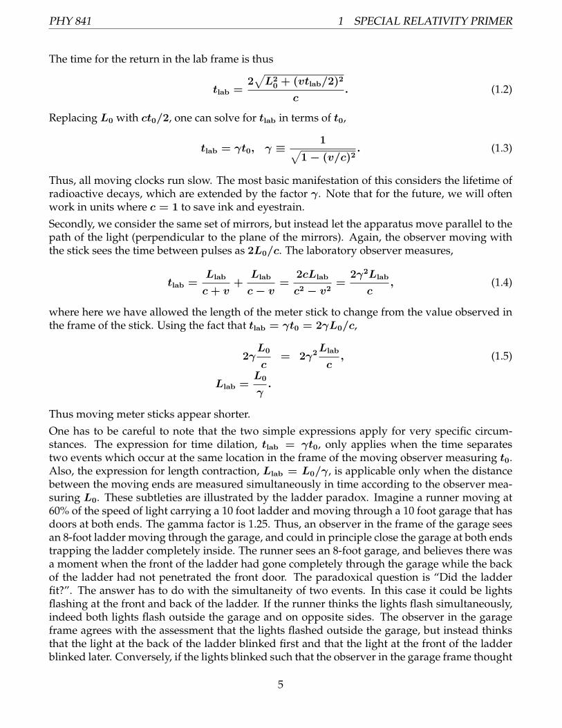
The time for the return in the lab frame is thus
tlab =2√L2
0 + (vtlab/2)2
c. (1.2)
Replacing L0 with ct0/2, one can solve for tlab in terms of t0,
tlab = γt0, γ ≡1√
1 − (v/c)2. (1.3)
Thus, all moving clocks run slow. The most basic manifestation of this considers the lifetime ofradioactive decays, which are extended by the factor γ. Note that for the future, we will oftenwork in units where c = 1 to save ink and eyestrain.
Secondly, we consider the same set of mirrors, but instead let the apparatus move parallel to thepath of the light (perpendicular to the plane of the mirrors). Again, the observer moving withthe stick sees the time between pulses as 2L0/c. The laboratory observer measures,
tlab =Llab
c+ v+
Llab
c− v=
2cLlab
c2 − v2=
2γ2Llab
c, (1.4)
where here we have allowed the length of the meter stick to change from the value observed inthe frame of the stick. Using the fact that tlab = γt0 = 2γL0/c,
2γL0
c= 2γ2
Llab
c, (1.5)
Llab =L0
γ.
Thus moving meter sticks appear shorter.
One has to be careful to note that the two simple expressions apply for very specific circum-stances. The expression for time dilation, tlab = γt0, only applies when the time separatestwo events which occur at the same location in the frame of the moving observer measuring t0.Also, the expression for length contraction, Llab = L0/γ, is applicable only when the distancebetween the moving ends are measured simultaneously in time according to the observer mea-suring L0. These subtleties are illustrated by the ladder paradox. Imagine a runner moving at60% of the speed of light carrying a 10 foot ladder and moving through a 10 foot garage that hasdoors at both ends. The gamma factor is 1.25. Thus, an observer in the frame of the garage seesan 8-foot ladder moving through the garage, and could in principle close the garage at both endstrapping the ladder completely inside. The runner sees an 8-foot garage, and believes there wasa moment when the front of the ladder had gone completely through the garage while the backof the ladder had not penetrated the front door. The paradoxical question is “Did the ladderfit?”. The answer has to do with the simultaneity of two events. In this case it could be lightsflashing at the front and back of the ladder. If the runner thinks the lights flash simultaneously,indeed both lights flash outside the garage and on opposite sides. The observer in the garageframe agrees with the assessment that the lights flashed outside the garage, but instead thinksthat the light at the back of the ladder blinked first and that the light at the front of the ladderblinked later. Conversely, if the lights blinked such that the observer in the garage frame thought
5

PHY 841 1 SPECIAL RELATIVITY PRIMER
they were simultaneous, the two lights could have both flashed inside the garage. However, therunner would have recorded the light at the front of the ladder blinking first.
The ladder paradox underscores the importance of thinking of times and distances as describingthe difference between two events, i.e., times and displacements are always relative to some-thing. There are other famous paradoxes in relativity that also lead to a better understandingof the essence of the theory, such as the twin paradox or whether the radius of a rotating wheelcontracts. However, the latter two involve acceleration and are thus related to the general theoryof relativity, which is not considered here, but would be considered in a course on gravity.
1.2 Lorentz Transformations
Space and time are even mixed together in non-relativistic (Newtonian) transformations. Forinstance, consider an event that occurs at time t and position x in the laboratory frame (Here weconsider only one spatial dimension). In a moving frame, the event occurs at:
xlab = x0 + vt0, tlab = t0, (1.6)
in a Newtonian transformation. For a relativistic transformation, we assume a more generallinear form,
xlab = Ax0 +Bvt0, (1.7)tlab = Ct0 +Dvx0, (1.8)
whereA,B,C andD are functions of v2. The powers of v are required by parity considerations.The inverse transformation should look the same, but with v → −v,
x0 = Axlab −Bvtlab, (1.9)t0 = Ctlab −Dvxlab.
First, we consider the decay of a relativistic particle which passes by the point (x = t = 0) inboth frames. Since the particle does not move in the particle frame (x0 = 0). The transforma-tions becomes
tlab = Ct0, (1.10)xlab = Bvt0.
The expression for time dilation in the previous section then yields,
C = γ. (1.11)
The decay occurs at the position xlab = vtlab, and since tlab = γt0, one finds
B = γ. (1.12)
To solve for the other two coefficients, consider the ladder paradox. Assume a light at the backend of the latter blinks at a time x = t = 0, and at the front end of the ladder a light blinkssimultaneously (in the frame of the ladder) at the space-time point, x0 = L0, t0 = 0. In the
6

PHY 841 1 SPECIAL RELATIVITY PRIMER
laboratory frame the lights blink at times different by an amount DvL0. The position at whichthe light blinks is
xlab = Llab + vtlab, (1.13)
where Llab is the length of the ladder. Since the apparent length of the ladder is shrunk by afactor γ, L.lab = x0/γ, and
xlab = x0/γ + vtlab, (1.14)
Rearranged,x0 = γxlab − γvtlab. (1.15)
This givesA = γ. To solve forD take the expressions, Eq.s (1.7,1.9,1.10) in the Lorentz transfor-mations, and solve forD. One findsD = γ.
The expressions for the coefficients defined in Eq.s (1.7-1.10)) can be summed up as a matrixequation,
rα = Lαβr
′β, (1.16)
L =
(γ γvγv γ
),
Here, the indices α are either 0 or 1, with “0” referring to time component and “1” referring tothe ‘x” component. If we included y and z, there would be four components representing thecoordinate of an event, t, x, y, z. These four components make up a “four-vector”. The Lorentzmatrix L performs a boost along the x axis and leaves the other two dimensions unchanged. Forour notes we will stick to the convention that greek indices label the components of four-vectors,while roman indices denote the components of three-vectors, i.e., α = 0, 1, 2, 3 and i = 1, 2, 3..The choice of making the indices upper vs. lower will be explained later.
For a boost along the x-axis, the 4 × 4 matrix becomes
L =
γ γv 0 0γv γ 0 00 0 1 00 0 0 1
. (1.17)
For rotations of a coordinate system, all three vectors are transformed according to the samerotation matrix U , r′i = Uijrj , regardless of whether the vector r refers to a spatial coordinateor a velocity or momentum. Similarly, for boosts all four-vectors are transformed the same,
rα = Lαβr
β, (1.18)
regardless of whether the quantity r represents the space-time coordinate of an event or a mo-menta (in which case the zero-th component is the energy).
Due to the identity, γ2 − γ2v2 = 1, one can express γ and γv as cosh η and sinh η respectively.The Lorentz matrix then becomes
L =
cosh η sinh η 0 0sinh η cosh η 0 0
0 0 1 00 0 0 1
, (1.19)
7

PHY 841 1 SPECIAL RELATIVITY PRIMER
which illustrates the similarity of the Lorentz transformations to rotations by an imaginary angle.
Whereas for a rotation, one finds that x1y1 + x2y2 + x3y3 = x · y is invariant to rotations,Lorentz transformations leave the quantity,
r · q ≡ r0q0 − r1q1 − r2q2 − r3q3 (1.20)
unchanged. To see this consider the the boosted quantities,
r′ = (γr0 − γvr1, γr1 − γvr0, r2, r3), (1.21)q′ = (γq0 − γvrq1, γrq1 − γvq0, q2, q3).
A little algebra shows that
r′0q′0 − r′1q
′1 − r′2q
′2 − r′3q
′3 = r0q0 − r1q1 − r2q2 − r3q3 (1.22)
= (γ2 − γ2v2)(r0q0 − r1q1) − r2q2 − r3q3
= r · q.
The “dot-product” of four vectors is as a Lorentz invariant, meaning a quantity unchanged byreference frame. The dot-product is also invariant to rotations in 3−space, and the combinationsof rotations and boosts is known as the Lorentz group. For a group, any combinations of transfor-mations can be expressed as a single transformation. If one adds parity and time-reversal, it isknown as the full Lorentz group, and if one adds translational symmetry, it becomes the Poincarégroup. Rotations and boosts are not in separable groups, i.e., if one performs two boosts, the re-sult is a boost plus a rotation. If the boosts had formed a group by themselves, any two boostswould have been equivalent to a single boost.
EXAMPLE:Consider two successive boosts along the x direction. The first defined by γv = sinh η1, andthe second one with γv = sinh η2. Show that the combination is equivalent to one boost withγv = sinh(η1 + η2).
Writing down the product of the two Lorentz matrices (2-dimensions is sufficient),(cosh η2 sinh η2sinh η2 cosh η2
)(cosh η1 sinh η1sinh η1 cosh η1
)=
(cosh η2 cosh η1 + sinh η2 sinh η1 cosh η2 sinh η1 + sinh η2 cosh η1cosh η2 sinh η1 + sinh η2 cosh η1 cosh η2 cosh η1 + sinh η2 sinh η1
)=
(cosh(η1 + η2) sinh(η1 + η2)sinh(η1 + η2) cosh(η1 + η2)
),
where double-angle formulas were applied for the last step. For high-energy phe-nomenology the the quantities η are referred to as “rapidities” when the boosts arealong the beam axis. The simplicity of rapidities comes from the fact that they addlike Newtonian velocities. However, this simple addition only works when the ra-pidities are defined along a single axis, i.e., if one defines sinh ηx = γvx, · · · , for allthree dimensions, the addition formulas break down due to the non-commutation ofboosts along different directions.
8

PHY 841 1 SPECIAL RELATIVITY PRIMER
1.3 Invariants and the metric tensor gαβ
As shown previously, the dot product of two vectors,
AαgαβBβ, (1.23)
gαβ ≡
1 0 0 00 −1 0 00 0 −1 00 0 0 −1
(1.24)
is invariant to both rotations and boosts. As a notional trick, one can define four-vectors Aα
(subscript rather than superscript) as
Aα ≡ gαβAβ, (1.25)
which means that AαAα is an invariant (summation of repeated indices inferred). In all calcu-lations the summed indices always appear with one superscript (contravariant) and one sub-scripted (covariant). The fact that multiplying by gαβ simply lowers the index also applies totensors, i.e.,
gαβCβγ = C γ
α . (1.26)
Note that this property means that gαβ is simply the unit matrix. Furthermore, this property alsoapplies to gαβ,
gαβCβγ = Cαγ. (1.27)
Derivatives might at first seem a little backwards. Consider a scalar function ϕ(x), where x is afour vector. For small changes in x, x
δϕ =∂ϕ
∂xµδxµ. (1.28)
Since δϕ is also a scalar, the vector ∂/∂xµ must transform as a covariant vector. This motivatesthe notation,
∂µ =∂
∂xµ. (1.29)
Note that for this convention, the equation of continuity is especially compact. For a four vectorJ , where J0 refers to the charge density and J i signals the current density, ∂ ·J = 0 → ∂tJ0+
∇ · J = 0. Maxwell equations also take on particularly beautiful forms, ∂αFαβ = Jβ, and
∂αFαβ = 0. Additionally, we point out that we will employ the convention throughout this
course that greek indices refer to all four components, while roman indices suggest only spatialcomponents. Bold face will refer to the vector components of a three-vector, while four-vectorswill not be put into bold face, i.e., p · x = p0x0 − p · x.
1.4 Four-Velocities and Momenta
For a particle that moves between two points by a small displacement ∆xα, one can define thequantity,
∆τ ≡√
∆xα∆xα, (1.30)
9

PHY 841 1 SPECIAL RELATIVITY PRIMER
which is an invariant. In the frame of the particle it is easy to see what this quantity represents,since in that frame the spatial components ∆xi are all zero. Thus ∆τ is the amount a clock,moving with the particle, has progressed during the differential displacement. Further, one candefine a vector,
uα ≡∆xα
∆τ, (1.31)
which is also a four-vector since ∆xα is a four-vector and ∆τ is a Lorentz scalar (or invariant).The four-vector uα is often referred to as the relativistic velocity, and given that ∆x0 = γ∆τ ,one can see that
u0 = γ, ui = γdxi
dt= γvi. (1.32)
It is easy to see thatuαuα = 1. (1.33)
The momentum is defined by multiplying uα by the particle’s mass m, which is also a scalar.This then gives,
pαpα = m2. (1.34)
The zeroth component of the momentum is identified as the energy. This gives the relation thatfor a particle at rest,
E = p0 = m. (1.35)
Of course, the more famous relation, E = mc2, requires keeping track of all the factors of c.
EXAMPLE:A beam of particles of mass mA is aimed a target with particles of mass mB. What kineticenergy,K, is required so that one can make a resonance of massmC .
The solution is based on energy-momentum conservation. One way to move forwardis to calculate the invariant mass in terms of the total momentum and set it tomC .
m2inv = (pA + pB)
2 = (K +mA +mB)2 − p2A
= (K +mA +mB)2 −
[(K +mA)
2 −m2A
]= m2
A +m2B + 2mB(K +mA) = m2
C,
K =m2
C − (mA +mB)2
2mB
.
EXAMPLE:Consider two particles recorded with momenta pA and pB at space times separated by rα =xα1 − xα
2 . In terms of relativistic invariants using pA, pB and r, solve for the impact parameter,i.e., the distance of closest approach as measured by an observer in the center-of-mass frame.
First, we consider two four vectors which will be used as projectors to eliminate thecomponents of r that, in the center-of-mass frame, are either time-like or along the
10

PHY 841 1 SPECIAL RELATIVITY PRIMER
direction of the relative momentum. First, the time-like vector is the total momen-tum,
Pα = pαA + pαB,
which in the c.o.m. frame becomes (EA + EB, 0, 0, 0). One can define a vector,
r′α ≡ rα − PαP · rP 2
.
In the center-of-mass frame, r′ looks exactly like r, except the α = 0 componentvanishes. Next, one defines a vector which in the c.o.m. frame is parallel to therelative momentum, and is zero for the α = 0 piece. This would be:
q′α = qα − PαP · qP 2
, qα = pαA − pαB.
Again, one can consider the c.o.m. frame, where it is clear that q′0 = 0 and q′i =(piA − piB). One can then project away the part of r′ parallel to q, and make a newvector b,
bα ≡ r′α − q′αq′ · r′
q′2
Finally, the impact parameter squared is, after some surprisingly painful algebra,
B2 = −b2 = −r2 +(q · r)2P 2 + (P · r)2q2 − 2(q · r)(P · r)(P · q)
P 2q2 − (P · q)2.
1.5 Examples of Invariants
Here I discuss several invariants you will encounter at various times throughout this course orin the literature. First, one can see that d4x is invariant to boosts by considering the Jacobian ofa Lorentz transformation along the x axis. In that case,
L =
cosh η sinh η 0 0sinh η cosh η 0 0
0 0 1 00 0 0 1
. (1.36)
The Jacobian is simply the determinant of the matrix, J = cosh2 − sinh2 = 1. Thus, d4x isinvariant. For a boost in an arbitrary direction, one can first to a rotation (d3x is invariant torotation) combined with a boost.
Then d4p is also invariant as is,∫d4p δ(p2 −m2)s(p) =
∫dp0d
3p δ(p20 − E2p)s(p) =
∫d3p
2Ep
s(p)|p0=Ep. (1.37)
11

PHY 841 1 SPECIAL RELATIVITY PRIMER
Here s(p) is some arbitrary scalar function. Since s could be anything, then one can state thatd3p/Ep is also invariant. This is why spectra in particle physics are expressed as one of the twoidentical forms below
EpdN
d3p=
dN
dϕptdptdy. (1.38)
The expression on the right-hand side can be found by seeing that dpz/E = dy, where y is therapidity. Since dN is the number of counts in a bin, and since a number of counts is invariant,you needn’t worry about how dN transforms.
Often, when calculating the number of particles in a box, one writes
N =
∫d3xd3p
(2π)3f(p), (1.39)
where f is the phase space density, or occupation probability. This must be an invariant. For in-stance, if you had fermions as zero temperature, f would be zero or unity depending on whetherit was inside or outside the Fermi sea. This would not change if viewed from a different referenceframe. Since f is invariant, and dN is invariant, it stands that d3x d3p is also invariant. To seethat this is true, one must remember that for this expression one assumes that dx measures thedistance between the boundaries of a cell where both the positions of the boundaries are mea-sured simultaneously, like measuring the length of a meter stick. If one compares the volumemeasured by an observer moving with the velocity of the particle, p/E, and compares to thelength in the lab frame one finds that d3x shorter by the Lorentz factor, E/m. If one considersd3p in the two frames, one sees that d3p in the lab frame must be larger by a factor of E/m sothat d3p/E is invariant. Thus, the product d3pd3x is invariant.
Another example that comes up often is a collision rate per volume and per time, dNc/d4x,
which is manifestly invariant. One can also consider the collision rate of particles from specificregions of momentum space, d3pa/Ea and d3p/Eb. The quantity would normally written as
EaEb
dNc
d4x d3pa d3pb= fa(pa)fb(pb)Something, (1.40)
where fa and fb are the phase space densities, or occupancies, of the two particles. Occupanciesare also invariant, i.e. if the Fermi sea is full, f = 1 regardless of what frame is considered.Here, Something has to be an invariant. Since it is invariant one can consider the center-of-mass frame where the momenta are back to back, pa = −pb. In that frame one knows fromkinematics that
Something =EaEb
(2π)6σ(
√s)vrel, (1.41)
where σ is the cross section and the relative velocity is vrel = |p|/Ea + |p|/Eb. One must thensimply write EaEbvrel as a Lorentz invariant. To do this,
EaEbvrel = paEb − pbEa|. (1.42)
One can now write Ea = pa · P/√s and replace pa with the spatial components of p′a ≡
pa − P (pa · P )/s to project out the zeroth components of pa. Doing the same for pb one then
12

PHY 841 1 SPECIAL RELATIVITY PRIMER
finds
(EaEbvrel)2 = − [(pb · P )(pa − P (pa · P )/s) − (pa · P )(pb − P (pb · P )/s)]2 /s
· · ·LOTS of algebra · · · (1.43)
=(s−m2
a +m2b)(s+m2
a −m2b)
4s
[s2 +m4
a +m4b − 2m2
am2b − 2sm2
a − 2sm2b
]=
(s−m2a +m2
b)(s+m2a −m2
b)
s
[(pa · pb)2 −m2
am2b
],
= wx
Here, numerous steps are omitted from the last step as this is related to a homework problem atthe beginning of the last chapter. Putting this all together, one finds
dNc
d4x=
∫d3pa
(2π)3Ea
d3pb
(2π)3Eb
fa(pa)fb(pb)σ(√s)√(pa · pb)2 −m2
am2b. (1.44)
1.6 Tensors
Tensors are quantities with two or more Lorentz indices. Examples are the stress-energy tensorand the electromagnetic field tensor. Similarly to how rotations in three-dimensional space affectthree-dimensional tensors,
M ′im = UijMjkU
−1Ukm, (1.45)
a relativistic tensor translates as
M ′αδ = LαβMβγL(−1)γδ. (1.46)
Again, note that summed indices always involve one covariant and one contravariant index. Sothe above equation can be rewritten a number of ways, e.g.
M ′αδ = LαβM γ
β L(−1)γδ. (1.47)
An example of a fourth-rank tensor is the anti-symmetric tensor,
ϵαβγδ =
1, for even permutations of αβγδ from 0123,
−1, for odd permutations of αβγδ from 0123,0, if any index repeats.
(1.48)
With these definitions,
ϵ0123 = ϵ1230 = ϵ2301 = ϵ3012 = ϵ0231 = ϵ2310 (1.49)= ϵ3102 = ϵ1023 = ϵ0312 = ϵ3120 = ϵ1203 = ϵ2031 = 1,
ϵ1023 = ϵ0231 = ϵ2310 = ϵ2310 = ϵ0132 = ϵ1320
= ϵ3201 = ϵ2013 = ϵ0213 = ϵ2130 = ϵ1302 = ϵ3021 = −1,
ϵαβγδ = 0 otherwise.
13

PHY 841 1 SPECIAL RELATIVITY PRIMER
1.7 Homework Problems
1. Suppose you are doing a fixed-target experiment at the LHC. The protons have a beamkinetic energy of 7 TeV. (The proton mass is 938.28 MeV/c2). If the experiment were redonewith a collider built with an equivalent center-of-mass energy, what would the kineticenergy of each beam be?
2. Find the equivalent fixed beam energy for a fixed target to have the same center-of-massenergy as the collider experiment at the LHC.
3. Consider a 1+1 dimension vector, (E, p), wherem2 ≡ E2−p2. Consider the transformedvector, p′α = Lαβp
β, where L is defined according to Eq. (1.19). Show that m′2 ≡ E′2 −p′2 = m2.
4. Consider two particles with four momenta pa and pb. Particle a is recorded at the spacetime point ra = (0, 0, 0, 0) and particle b is recorded at rb = r. For an observer movingwith particle a find the time at which particle b passes at the point of closest approach.Express your answer in terms of Lorentz invariants, i.e., dot products involving pa, pb andr.
5. Consider two particles of mass ma and mb with four momenta pa and pb. Show that therelative velocity, |va − vb|, according to an observer in the center-of-mass frame is:
v2rel =s2/4
(pa · P )2(pb · P )2
[s2 +m4
a +m4b − 2sm2
a − 2sm2b − 2m2
am2b
].
Here, P is the total momentum and s = P 2. FYI: The answer is sometimes called thetriangle function. If you have a triangle with sides of length (
√s,ma,mb) and solve for
the area of the triangle you get a similar function aside from the prefactor. This term forthe relative velocity appears often, e.g. you divide by this factor to convert rates fromFeynman diagrams into cross sections.
6. The Lorentz transformation is a tensor, Lαβ, which transforms some four vector pα ob-served by an observer moving with four velocity uα to a vector p′α as determined by anobserver moving with four-velocity u′α.
Lαβp
β = p′α.
Since L is a tensor it must be of the form,
Lαβ = Auαu′β +Bu′αuβ + Cuαuβ +Du′αu′β + Egαβ, (1.50)
whereA−E are scalar functions of u and u′. Since u2 = u′2 = 1, the only scalar functionavailable is u · u′. Consider the transformation from the rest frame u = (1, 0, 0, 0) to theframe u′ = (γ, γv, 0, 0). You know that the Lorentz transformation is:
Lαβ =
γ −γv 0 0
−γv γ 0 00 0 1 00 0 0 1
.14

PHY 841 1 SPECIAL RELATIVITY PRIMER
Further, u · u′ = γ. From the form in Eq. (1.50),
Lαβ =
Aγ +Bγ + C +Dγ2 + E −Aγv −Dγ2v 0 0
Bγv +Dγ2v −Dγ2v2 + E 0 00 0 E 00 0 0 E
.(a) Solve for the coefficientsA through E in terms of γ = u · u′.
(b) Show that for the four vector u′,
Lαβu′β = uα.
(c) Show thatLαβ(u, u′)Lβγ(u
′, u) = gαγ.
15

PHY 841 2 DYNAMICS OF RELATIVISTIC POINT PARTICLES
2 Dynamics of Relativistic Point Particles
We won’t discuss the dynamics of individual charged particles very much in this course, butit is good to review the least-action principle, and the example for relativistic particles. In thenext chapter we will apply these principles to field equations, deriving Maxwell’s equations,so it will be helpful to review the connection between least action and Lagrange’s equations,with an emphasis on how symmetries lead to conservation laws. In this chapter we consider theinteraction with an external electromagnetic field. This chapter closely follows the approach inLandau and Lifshitz.
2.1 Lagrangian for a Free Relativistic Particle
The action, S, is related to a Lagrangian by
S =
∫ tb
ta
dt L(r(t), ˙r(t), t). (2.1)
Usually, there L has no explicit dependence on t and only depends on r and ˙r. In that caseminimizing S leads to Lagrange’s equations,
δS =
∫ tb
ta
dt∑i
(∂L∂ri
δri +∂L∂ri
δri
)(2.2)
=
∫ tb
ta
dt∑i
(−d
dt
∂L∂ri
+∂L∂ri
)δri
= 0.
The equivalence must be true for any δri at any time, thus one derives the usual Lagrangeequations of motion,
d
dt
∂L∂ri
δri =∂L∂ri
. (2.3)
If there are symmetries, in that L does not depend on some coordinate, a conservation lawensues. For instance, if L is independent of ϕ (but not ϕ) the rotational symmetry gives,
d
dt
∂L∂ϕ
= 0, (2.4)
and pϕ = ∂L/∂ϕ is conserved. More generally, consider any small change xi → x + ϵi(x, t).For translational invariance ϵ is independent of x and δxi = ϵi(t), and setting δS = 0, onefinds
δS = 0 (2.5)
= −∫ tb
ta
dtd
dt
∂L∂xi
ϵi(t).
16
PHY 841 2 DYNAMICS OF RELATIVISTIC POINT PARTICLES
Thus ∂L/xi is conserved, and is the momentum in the i direction. For rotational invarianceabout an axis Ω, δxi = ϵijkxjΩkδϕ(t),
δS = 0 (2.6)
= −∫ tb
ta
dtd
dt
∂L∂xi
ϵijk(t)xj(t)Ωkδϕ(t).
This must be true for any small angle δϕ, and the conserved quantity is known as the angularmomentum vector about the Ω axis.
LΩ = −∂L∂xi
ϵijkxj(t)Ωk (2.7)
= (r × p) · Ω.
If there exists rotational invariance about any axis then all three components of L are conserved.
The connection between symmetries and conservation laws is as important a concept as anyin all of physics. For example, in quantum field theory, the arbitrary phase of a complex fieldoperator is related to conservation of electric charge.
Conservation of energy comes from Lagrange’s equations. Defining πi ≡ ∂L/∂qi, where qi arethe generalized coordinates,
d
dt(πiqi − L) = πiqi + πiqi −
∂L∂qq −
∂L∂qi
qi (2.8)
= 0.
Thus, the Hamiltonian H = πiqi − L is conserved. Note this was contingent on the lack ofexplicit time dependence in L. Thus, invariance under translation in time is associated withenergy conservation.
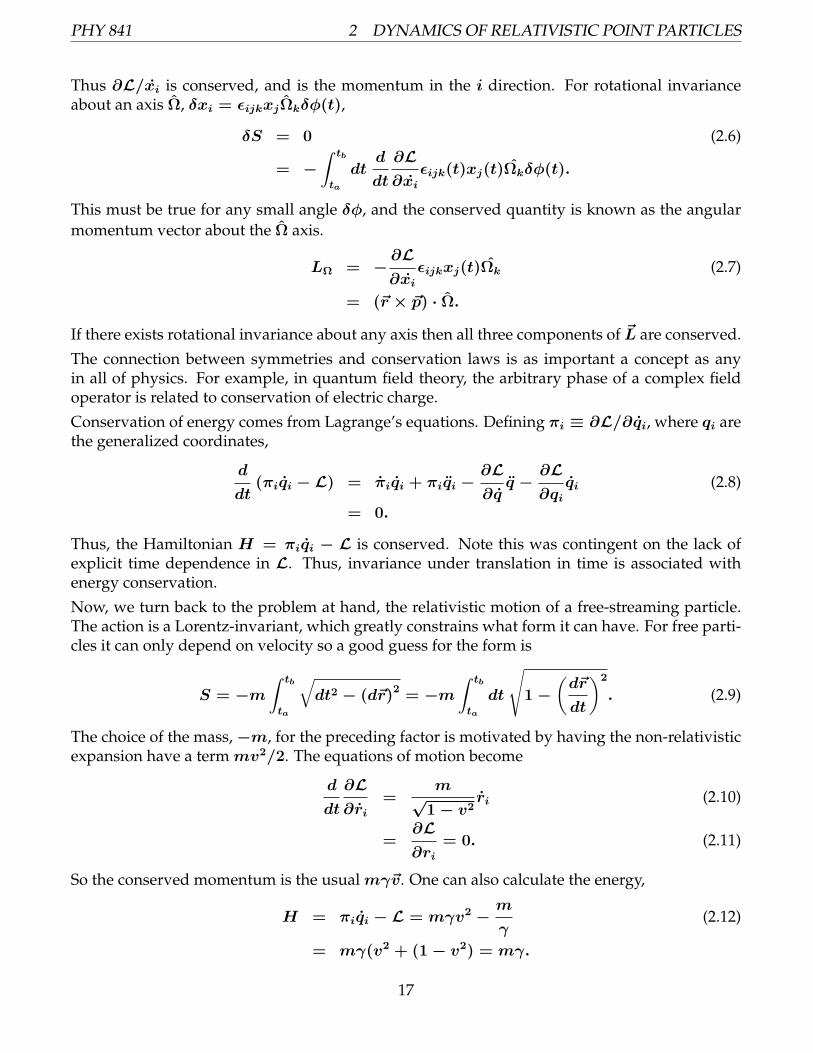
Now, we turn back to the problem at hand, the relativistic motion of a free-streaming particle.The action is a Lorentz-invariant, which greatly constrains what form it can have. For free parti-cles it can only depend on velocity so a good guess for the form is
S = −m∫ tb
ta
√dt2 − (dr)2 = −m
∫ tb
ta
dt
√1 −
(dr
dt
)2
. (2.9)
The choice of the mass, −m, for the preceding factor is motivated by having the non-relativisticexpansion have a termmv2/2. The equations of motion become
d
dt
∂L∂ri
=m
√1 − v2
ri (2.10)
=∂L∂ri
= 0. (2.11)
So the conserved momentum is the usualmγv. One can also calculate the energy,
H = πiqi − L = mγv2 −m
γ(2.12)
= mγ(v2 + (1 − v2) = mγ.
17

PHY 841 2 DYNAMICS OF RELATIVISTIC POINT PARTICLES
Of course, if you included the factors of cwe would get E = mc2 for v = 0.
Boost symmetries are a bit more difficult to consider due to the mixing of time and position. Thebest way to consider these is to define t = r0 and r in one frame, then consider the boost ofsmall velocities or rotations
r′α = rα + δΩαβ(t)rβ. (2.13)
Here, the tensor Ωαβ is any anti-symmetric tensor. The three 0i elements represent boosts, whilethe three non-zero ij elements represent rotations.
Now, we rewrite the Lagrangian and action as
S = −m∫ tb
ta
dt
√(dt′
dt
)2
−(dr′
dt
)2
. (2.14)
For δv = 0 the coordinates are t′ = t, r′i = ri, which gives the usual answer. For small δv,
δS =
∫ tb
ta
dt∂L∂rα
d
dt
(δΩαβrβ
)(2.15)
=
∫ tb
ta
dt
[−d
dt
(∂L∂rα
rβ
)+
(∂L∂rα
)rβ
]δΩαβ
=
∫ tb
ta
dt
[−d
dt(παrβ) + παrβ
]δΩαβ
= 0.
The second term disappears because δΩαβ is anti-symmetric and π is parallel to r. This must bezero for any contribution from given components δΩαβ and δΩβα = −δΩαβ,
d
dt
(rαpβ − pαrβ
)= 0, (2.16)
for any choice of αβ. For αβ both with space-like indices, these components correspond toangular momenta.
Mαβ = rαpβ − pαrβ, (2.17)M12 = Lz, M
23 = Lx, M31 = Ly.
For the components with α = 0,
M01 = tpx − xE, M02 = tpy − yE, M03 = tpz − zE. (2.18)
Each of the six elements represent conserved quantities. For theM0i elements the quantities rep-resent the fact that the center-of-mass moves with fixed velocity. If there were several particlesthe quantities would be ∑
a
(pat− rEa) = constant. (2.19)
18

PHY 841 2 DYNAMICS OF RELATIVISTIC POINT PARTICLES
Dividing the equation by the conserved energy, Etot =∑
aEa, one gets(∑a pa
Etot
)t −
∑aEara
Etot
= constant. (2.20)
Thus the center of mass is defined as an average sum over the positions weighted by their en-ergies, and it moves with constant velocity Ptot/Etot. Of course, all this is postulated on theLagrangian not having interactions that might destroy the Lorentz invariance assumed above.
2.2 Interaction of a Charged Particle with an External Electromagnetic Field
Here, the external electromagnetic field is a four-vector Aµ(r). The zeroth component is theelectric potentialϕ and the spatial components are the usual vector potential. To make a Lorentz-invariant action that has a contribution that looks like the usual potential energy, eϕ(r), weconsider
S =
∫dτ (−m− eu ·A) (2.21)
= −m∫dt
√(dt′
dt
)2
−(dr′
dt
)2
− e
∫dt(A0 − v · A
).
Here, we have used the fact that u0dτ = γdτ = dt and udτ = vdt. The conjugate momenta ischanged by the appearance of the velocity in the v · A term,
π = mγv + eA. (2.22)
Lagranges equations then become
d
dt(mγvi + eAi) = −e∂iA0 + ev∂i · A (2.23)
d
dtmγvi = −e∂tAi − e∂iA0 − ev · ∇Ai + ev∂i · A.
Here, we have made use of the fact that d/dt = ∂t + v · ∇. Next, the last two terms can bemanipulated with the vector identity,
A× (B × C) = B(A · C) − C(A · B), (2.24)d
dt(mγvi) = −e∂iA0 − e∂tAi + ev × (∇ × A).
Thus, the electric and magnetic fields are
E = −∇A0 − ∂tA, (2.25)B = ∇ × A,
and the equations of motion are
d
dt(mγvi) = eE + ev × B. (2.26)
19

PHY 841 2 DYNAMICS OF RELATIVISTIC POINT PARTICLES
The electric potential is the zeroth component of the four-vector potential. It is NOT a scalar.Since the four components of A mix during a boost, magnetic and electric fields also mix. Con-sider a frame where there is a constant electric field in the z direction due to a potential,
A0 = −zE, A = 0. (2.27)
If one boosts in the x direction by a velocity v,
A′0 = γ(−zE), (2.28)A′x = γv(−zE).
Using the fact that z = z′ for a boost along the x axis, the ensuing electric and magnetic fieldsare
E′ = γEz, (2.29)B′ = ∇ × A′ = −vEy.
2.3 Motion in a Constant Magnetic Field
Let’s consider the gauge where
A = xBy, (2.30)
which gives B = Bz. Beginning with the action, we solve Lagrange’s equations
S = −∫dtm√1 − v2 − exBvy
, (2.31)
py = mγvy + eBx, = constant because there is no y dependence,
px = mγvx,d
dtpx = eBvy. (2.32)
Now, let’s show that is indeed circular motion. We need to show that these equations (clockwisecircular motion) are satisfied by
x = x0 +R cos(ωt− ϕ), (2.33)y = y0 −R sin(ωt− ϕ),
vx = −ωR sin(ωt− ϕ),
vy = −ωR cos(ωt− ϕ).
From the equation for dpx/dt one sees that
ω =eB
mγ, (2.34)
which is the usual expression for the cyclotron frequency except for the 1/γ factor. Note this iswhy cyclotrons can’t work for relativistic energies.
20

PHY 841 2 DYNAMICS OF RELATIVISTIC POINT PARTICLES
Next, we must show that py is indeed a constant.
py = −mγV cos(ωt− ϕ) + eBx, (2.35)= −mγωR cos(ωt− ϕ) + eB(x0 +R cos(ωt− ϕ))
= eBx0. This emphasizes that p in not the velocity multiplied by the mass, but differs by eA. So havingpy being a constant does not mean that the y-component of the velocity is fixed.
2.4 Gauge Transformations
Consider the following change to the vector potential,
A′µ = Aµ + ∂µΛ(t, x, y, z). (2.36)
Here Λ is a arbitrary scalar function. The electric and magnetic fields become (with the use ofEq. (2.40))
E′i = Ei − ∂i∂tΛ + ∂t∂iΛ = Ei, (2.37)
B′i = Bi − ϵijk∂j∂kΛ = Bi. (2.38)
Thus, E and B are unchanged by the function Λ, even though A is changed. This is knownas gauge invariance. In nature, the fields A are indeed physical when one considers quantummechanics, e.g. the Aharonov-Bohm effect. However, even then gauge invariance is still true thescalar function Λ is arbitrary.
2.5 The Electromagnetic Field Tensor
One can define a second-rank anti-symmetric tensor using the vector potential,
Fαβ = ∂αAβ − ∂βAα. (2.39)
Using the definitions,
E = −∂tA− ∇A0, (2.40)B = ∇ × A,
one can consider Fαβ component-by-component and find
Fαβ =
0 Ex Ey Ez
−Ex 0 −Bz By
−Ey Bz 0 −Bx
−Ez −By Bx 0
, Fαβ =
0 −Ex −Ey −Ez
Ex 0 −Bz By
Ey Bz 0 −Bx
Ez −By Bx 0
. (2.41)
The equations of motion then take the form (see HW problem),
md
dτuα = eFαβuβ, (2.42)
where dτ =√dt2 − (dr)2, is the differential time step in the frame of the particle, i.e. its proper
time.
21

PHY 841 2 DYNAMICS OF RELATIVISTIC POINT PARTICLES
2.6 Homework Problems
1. Consider a system of free particles awith the Lagrangian set as
L = −ma
∑a
√(dt′adt
)2
−(dr′adt
)2
, (2.43)
with t′a = t before transforming. Now consider a translation in time,
t′a = t+ ϵ(t), r′a = ra.
Calculate δS and express it so that δS is proportional to ϵ(t), not ϵ. Show that this quicklygives energy conservation.
2. Consider a particle of charge e and mass m moving in a constant electric field in the xdirection,A0 = −eEx. The particle’s initial momentum is p(t = 0) = pyy.
(a) Solving Lagrange’s equation, find px(t).
(b) Using the fact that vx = px/√m2 + p2x + p2y, find x(t).
(c) Using the fact that vy = py/√m2 + p2x + p2y, find y(t).
(d) Find the trajectory, x(y).
(e) Take the limit py/m << 1 and find x(y) again. Solve non-relativistically and com-pare.
3. Consider a particle of charge e and mass m moving in a constant magnetic field in the zdirection. We will consider the gauge where,
Ay = xB/2, (2.44)Ax = −yB/2, (2.45)
A =Bρϕ
2. (2.46)
Here, ρ =√x2 + y2 and ϕ = y cosϕ − x sinϕ is one of the three unit vectors in the
cylindrical coordinate basis, z, ρ, and ϕ.
(a) Find the scalar function Λ that transforms the choice used in the earlier section, A =xBy to the vector potential used here.
(b) Find pϕ = ∂L∂ϕ
.
(c) Setting z = 0, consider motion in the x − y plane. Beginning with (d/dt)πϕ = 0,show that the solution with fixed radius (ρ = 0) will work if the ϕ is constant and isrelated to the cyclotron frequency as shown in the previous subsection,
ϕ =eB
mγ.
22

PHY 841 2 DYNAMICS OF RELATIVISTIC POINT PARTICLES
4. Consider a particle of massmmoving in a scalar field, Φ(r) = −Fx. This simply changesthe local mass tom = m0 − Fx, and the Lagrangian is
L = −(m0 − Fx)√
1 − v2.
The mass changes with time as m = m0 − Fx, and dm/dt = −vF , where v will be thevelocity in the x direction. For the questions below, assume there is no movement in the yor z directions.
(a) Using Lagrange’s equations, show
dv
dt= (1 − v2)
F
m(t).
(b) Consider a particle at rest at x = y = z = t = 0. Show that the solutions to theabove equations are
m = m0 cos(at), a = F/m0
v = sin(at),
x =1
a(1 − cos(at)).
(c) At what time, tmax, does the mass become zero?
(d) What is x(tmax)?
(e) What is v(tmax)?
(f) What is ux = γv at tmax?
5. It is easy to derive the spatial components of Eq. (2.42),
d
dτpi = qF iαuα,
by expressing Fαβ in terms of E and B using Eq. (2.41), then comparing the Eq. (2.26). Itis less obvious to see how one obtains the equation for d/dτp0. Given that p0 = mγ, onecan quickly see that
d
dτp0 = ev ·
d
dτp.
Beginning with the two expressions above, show that
d
dτp0 = qF 0βuβ.
Hint, you will need to use the fact that Fαβ is anti-symmetric.
23

PHY 841 3 DYNAMIC ELECTROMAGNETIC FIELDS
3 Dynamic Electromagnetic Fields
So far we have discussed the motion of particles in a field, but have ignored how the fields mightchange in time. To do so, we need to consider all three parts of the action: the action of a freeparticle, Sm, the action involving the interaction of matter with the field Sfm and, new for thischapter, the action of the field, Sf . We will show how this action leads to Maxwell’s equations.
3.1 Lagrangian (Density) for Free Fields: Deriving Maxwell’s Equations
In the last chapter we considered the motion of a particle in a field, Aα(r), where the field wasgiven as a function of time. First we will derive Maxwell’s equations, which describe how thefield responds to the current and how it evolves. For the moment, we ignore the external currentsand look at Sf ,
Sf =
∫d4rL(Aµ, ∂νA
µ), (3.1)
where A and ∂νA are functions of the four-position r. Here L is not actually the Lagrangian,it is the Lagrangian density, and
∫d3rL is the Lagrangian. However, people typically refer to
it as the Lagrangian anyway. A difference between the Lagrangian for a point particle is thatL is a function of all four derivatives, ∂tA
µ, ∂xAµ, ∂yA
µ and ∂zAµ. Again, we start with the
condition of minimizing the action,
δS =
∫d4r
(∂µδA
ν)∂L
∂∂µAν+ (δAν)
∂L∂Aν
(3.2)
=
∫d4r δAν
−∂µ
∂L∂∂µAν
+∂L∂Aν
.
Minimizing the action gives Lagrange’s field equations,
∂µ
∂L∂∂µAν
=∂L∂Aν
. (3.3)
Again, this assumes that L has no explicit dependence on r, as it only depends on r through itsdependence onA and derivatives ofA. The only visual difference between the usual Lagrangianequations and what we see here is that d/dt is replaced by ∂µ.
Our next step is to write the Lagrangian density for free fields. The form must be Lorentz invari-ant, and must ultimately lead to the usual expressions for the energy density. Another criteriais that it is gauge-invariant, i.e. that it should depend only on F µν , and not A. The choice thatworks is
L = −1
16πF µνFµν =
1
16πF µνFνµ. (3.4)
24

PHY 841 3 DYNAMIC ELECTROMAGNETIC FIELDS
The last step used the fact that F µν = ∂µAν − ∂νAµ is anti-symmetric. From Lagrange’s fieldequations, Eq. (3.3),
∂µ
∂L∂∂µAν
=1
16π∂µ
∂
∂∂µAν(∂αAβ − ∂βAα)(∂αAβ − ∂βAα) (3.5)
=1
4π∂µ (F µν) = 0.
If one adds the interaction between the fields and particles,
Sfm =
∫d4r J ·A, (3.6)
Lagrange’s field equations then become
1
4π∂µ (F µν) = Jν. (3.7)
Here, the current Jα is the current density which is a four-vector. For charged particles movingin a small volume Ω,
Jα =1
Ω
∑a∈Ω
qauα
a
γa. (3.8)
For J0 this u0/γ = 1 and one sees that J0 is the charge density. For the spatial components,u/γ = v and one sees that J i is the current density. One can also check to see that Jα(r) is afour-vector by writing it as
Jα(r) =∑a
∫dτa δ
4(ra − r)qauαa , (3.9)
=∑a
δ3(ra(r0) − r)qau
αa
γ.
If one averages this over some small volume Ω by integrating over the volume and dividing byΩ, one obtains Eq. (3.8). Thus, Eq.s (3.8) and (3.9) are equivalent expressions of the four-current.
Using Eq. (2.41) to express F µν in terms of E and B, these four equations (one equation for eachvalue of ν) then become
∇ · E = 4πJ0, (3.10)(∇ × B) − ∂tE = 4πJ.
The zeroth component of the current is the charge density, so this are simply a statement of twoof Maxwell’s equations. To obtain the other two equations we consider the tensor
F µν =1
2eµναβFαβ, (3.11)
25

PHY 841 3 DYNAMIC ELECTROMAGNETIC FIELDS
with F known as the dual electromagnetic tensor. One can them see that
∂µFµν = −
1
2ϵνµαβ∂µ(∂αAβ − ∂βAα) (3.12)
= 0.
Equating to zero comes from the fact that two derivatives, ∂µ∂α or ∂µ∂β, are contracted throughthe Levi-Civita tensor, which being anti-symmetric must cancel the contribution from the deriva-tives. Using Eq. (2.41) one can see that
Fαβ =
0 −Bx −By −Bz
Bx 0 −Ez Ey
By Ez 0 −Ex
Bz −Ey Ex 0
. (3.13)
Expressing Eq. (3.12) in terms of E and B,
∇ · B = 0, (3.14)∂tB + ∇ × E = 0.
Summarizing, Maxwell’s equations in covariant notation are
∂αFαβ = 4πJβ, (3.15)
∂αFαβ = 0.
For a point charge within a sphere of radiusR, Gauss’ law says that
4π
∫d3r J0 +
∮dA · E. (3.16)
Using symmetry, E = Er, and combined with the recognition that integrating the charge den-sity inside the sphere gives the charge
Q =
∫d3rJ0, (3.17)
one finds
4πQ = 4πR2E, (3.18)
E =Q
R2.
Compared to the expressions of Coulomb’s law to which one is usually accustomed, there isno 4πϵ0 in the denominator or constant k in the denominator. This is due to the way in whichcharge is defined. For example, if you read texts in nuclear physics you will typically find theCoulomb energy for a proton near a nucleus of atomic number Z written as
PE =Ze2
r. (3.19)
26

PHY 841 3 DYNAMIC ELECTROMAGNETIC FIELDS
If one wishes the energy to be in MeV, and the radius r to be in Fermi (aka femtometers), oneuses the fact that
e2 =ℏc
137.036, (3.20)
where e2/ℏc = 1/137.036 is known as the fine structure constant, which is dimensionless, andℏc = 197.327 MeV fm. In other fields one might more typically see a more arbitrary definition ofcharge, e.g. Coulombs. In such cases, Coulomb’s law must then be modified by some prefactor,e.g. 1/4πϵ0.
3.2 Pseudo-Vectors and Pseudo-Scalars
The vector potential Aα is a four-vector, and the field tensor Fαβ is a second-rank tensor. Theelectric field E = −∇A0 + ∂tA is a 3-vector, but one that transforms as part of a tensor if thetransformation involves a boost. The magnetic field B = ∇×A is a pseudo-vector. The "pseudo"comes from the fact that its definition, Bi = ϵijk∂jAk, involves two-vectors, so even though ithas only one vector index, it does not switch sign under parity (x → −x, y → −y, z → −z).Tensors can behave rather strangely under parity because some of the elements don’t changeunder parity while others do. One can define the pseudo-scalar
FαβFαβ = −4E · B. (3.21)
Like scalars, this is manifestly invariant under Lorentz transformation, however it is odd underparity. This can also be written as
FαβFαβ =1
2ϵαβγδFαβFγδ (3.22)
=1
2ϵαβγδ(∂αAβ)(∂γAδ).
Each term has a product of four four-vector components, one being a zeroth component and theother three being spatial. Thus, this quantity is odd under parity.
Finally, another obvious example of a scalar, which is even under parity, is
FαβFαβ = −2(|E|2 − |B|2). (3.23)
Thus, although E and B mix under boosts, the difference of their magnitudes remains fixed.
The sign of a pseudo-vector or pseudo-scalar changes if one changes from a right-handed toa left-handed coordinate system. This is because ϵijk was arbitrarily defined so that ϵxyz waspositive. Even though magnetic forces feature pseudo-vectors, the interaction conserves parity,i.e. it does not matter whether you used a right-handed or left-handed coordinate system. Thisis because the force, which is something you can observe, behaves as ∇ × B, Fi = qϵijkvjBk.Thus, in considering a force, the Levi-Civita symbol appears twice, once in defining B and oncein defining the force. Thus, one would see the same effect using a left-handed coordinate system.
The weak interaction does not conserve parity. If one aligns a nucleus so that its angular mo-mentum, which is a pseudo-vector, points along the positive z, and if that nucleus undergoes
27

PHY 841 3 DYNAMIC ELECTROMAGNETIC FIELDS
a weak-interaction decay (beta decay), the electrons are emitted with strong preference parallelto the angular momentum. This violates parity because the direction of the electrons is real, itmakes a difference if the electrons go up vs. down, but the direction of the angular momen-tum (or the magnetic field used to polarize the atoms) is a pseudo-vector and dependent on theright-handed vs. left-handed choice of coordinate system.
3.3 The Stress-Energy Tensor of the Electromagnetic Field
Just like the energy, H = πq − L, is conserved for a usual Lagrangian, one can define a sim-ilar quantity for the Lagrangian density. However, this quantity will be a second-rank tensorand will express local conservation of both energy and momentum. Just to reduce the indexoverload, we consider a function L(ϕ, ∂αϕ). We can replace ϕ with Aµ, but essentially theproof will be the same aside from summing over each of the four fields Aµ. First, we define thestress-energy tensor Tαβ,
Tαβ = πα∂βϕ− gαβL, (3.24)
πα ≡∂L
∂(∂αϕ)
When α = β = 0, this looks like the usual definition of energy, except this is the Lagrangiandensity so T 00 has dimensions of energy per length cubed. To see how this is related to a con-served quantity, consider
∂αTαβ = (∂απ
α)(∂βϕ) + πα(∂α∂βϕ) −
∂L∂ϕ
∂βϕ−∂L
∂(∂αϕ)∂α∂
βϕ. (3.25)
The first and third terms vanish via Lagrange’s field equations, Eq. (3.3), and the second andfourth terms cancel via the definition of the conjugate momentum, πα, in Eq. (3.24). Thus,
∂αTαβ = 0. (3.26)
Any function Jµ that satisfies the equation of continuity ∂µJµ = 0 implies that J is a conserved
current density. For such a four-vector, the zeroth component is the charge density and the threespatial components J i are current densities. The conservation ensues because
∂t
∫d3rJ0 = −
∫d3r∇ · J . (3.27)
The latter terms vanishes because the currents vanish at infinity so the net charge Q =∫d3rJ0
is conserved. The conservation is local because if one considers a small volume, the change inthe charge equals the flux of current through the boundary, also seen via the divergence theorem(aka Gauss’ law). The “charge” needn’t be electric charge but any conserved quantity.
In our case, for each value of β in Tαβ one has a conserved four-current. Thus, T 00, T 01, T 02 andT 03 represent densities of conserved quantities. Those quantities are the energy and momentumdensities. The quantities T 10, T 20 and T 30 represent the flux of energy density, i.e.
∂t
∮d3r T00 = −
∮dA · J , Jα = Tα0. (3.28)
28

PHY 841 3 DYNAMIC ELECTROMAGNETIC FIELDS
The three quantities T 0i represent momentum densities. It is not obvious, but the stress-energytensor is symmetric, and the flux of the energy, T i0 equals the momentum density, T 0i. To provethe symmetry once must consider the effect of an asymmetric term (further ahead). In this casethe one finds an infinite angular acceleration, and angular momentum is not conserved.
The other nine components of the stress-energy tensor represent the flux of momentum. Forexample, the quantity T xydSy represents the rate momentum Px flows through a surface ele-ment of area dSy which points in the y direction. This would be a shear. In hydrodynamics, thisvanishes and in the frame of the fluid (where T 0i = 0) T ij = Pδij , where P is the pressure.For field equations, the spatial components T ij simply represent momentum fluxes and can bequite complicated, thought the tensor does have to remain symmetric.
Now, to return to the specific case of the electromagnetic field. In that case, the quantities πα
and Tαβ discussed above are functions of four fields and to express the conjugate momenta orthe stress-energy tensor, one must simply extend the above relations to sums over all four fields.There are four conjugate momenta for each field, and becauseAα is effectively four fields, thereare four conjugate momenta for each α and the momenta are represented by a four-by-fourtensor.
παβ =∂L
∂(∂αAβ), (3.29)
Tαγ = παβ∂γAβ − gαγL.
Using L = − 116πFαβFαβ,
παβ =−1
4πFαβ, (3.30)
Tαγ =−1
4πFαβ∂γAβ +
1
16πgαγF µνFµν.
However, as previously stated the stress-energy tensor should be symmetric. To make it sym-metric, we add a derivative of the form ∂µG
µ, which by Gauss’s law will integrate to zero ifone considers all space. Thus if we add the term, (1/4π)∂β(F
αβAγ), the stress-energy tensorbecomes
Tαγ =−1
4πFαβ∂γAβ +
1
16πgαγF µνFµν +
1
4π∂β(F
αβAγ) (3.31)
=1
4πFαβF γ
β +1
16πgαγF µνFµν +
1
4π(∂βF
αβ)Aγ.
The last term vanishes for free fields because ∂αFαβ = 0 when there are no currents present, so
Tαγ =1
4πFαβF γ
β +1
16πgαγF µνFµν. (3.32)
In addition to being symmetric, the tensor is traceless, Tαα = 0. Expressing the components in
29

PHY 841 3 DYNAMIC ELECTROMAGNETIC FIELDS
terms of E and B,
T 00 =1
8π(E2 +B2), (3.33)
T 0i =1
4πϵijkEjBk,
T ij = −T ij =
1
8π(δij(E
2 +B2) − 2EiEj − 2BiBj).
The momentum density, or energy flux is T 0i or writing the three components as a vector, (E ×B)/4π. This is known as the Poynting vector.
To explain why the stress-energy tensor must be symmetric, consider an infinitesimal cube ofdimension a × a × a. Consider rotation about the z axis. The shear forces, Ti =j , contributeto the angular momentum. The forces on the four sides due to Txy and Tyx are Tyxa
2x on theupper face, −Tyxa
2x on the lower face, a−Txya2y on the right face and Txya
2y on the left-sideface. The net torque is thus
τ = a3(Tyx − Txy). (3.34)
However, the moment of inertia scales as a5, so the angular acceleration would scale as 1/a2 →∞, unless the tensor is anti-symmetric. To understand why T0i = Ti0, one can consider a boost.Under boosts, any such asymmetry would translate into an asymmetry in the ij components.
One can also show explicitly that the stress-energy tensor is conserved in the presence of in-teractions with currents. Beginning with the definition for the field contribution, T (f), in Eq.(3.32),
T (f)αβ =1
4πFαγF β
γ +1
16πgαβF µνFµν, (3.35)
∂αT(f)αβ =
1
4π(∂αF
αγ)F βγ +
1
4πFαγ∂αF
βγ +
1
8πFαγ∂βFαγ,
= JγF βγ +
Fαγ
4π
(∂α∂γA
β − ∂α∂βAγ +
1
2∂β∂αAγ −
1
2∂β∂γAα
)= JγF β
γ +Fαγ
4π
(∂α∂γA
β −1
2∂β∂αAγ −
1
2∂β∂γAα
)The terms inside the parenthesis vanish because they are explicitly symmetric in the αγ indices,which when contracted with the anti-symmetric tensor Fαγ , must vanish. Thus,
∂αT(f)αβ = JγF
γβ. (3.36)
Next, we consider the contribution to the stress energy tensor from the matter contribution. Todo this we consider matter to have a mass density
µ(r) =∑a
maδ(r − ra), (3.37)
which given that the total mass is conserved, for free particles, one can write a conserved masscurrent,
J0 = µ(r), (3.38)
Jα(r) =∑a
maδ(r − ra(r0))uα(r)/u0(r).
30

PHY 841 3 DYNAMIC ELECTROMAGNETIC FIELDS
To see that J is indeed a four-vector, one could write
Jα(r) =∑a
ma
∫dτaδ(r0 − ta)δ(r − ra(ta))u
αa (3.39)
=∑a
maδ(r − ra(r0))uαa/γa
=∑a
maδ(r − ra(r0))uα(r)/u0(r).
Here, the four-velocity dependence on r is some complicated function that has the correct veloc-ity for each particle awhen r = ra. The mass current is conserved, ∂ · J = 0. The stress energytensor can be written as
T (m)αβ(r) = Jα(r)uβ(r), (3.40)∂αT
(m)αβ = (∂ · J)uβ + (J · ∂)uβ(r).
The first term vanishes due to current conservation, and the second term becomes
∂αT(m)αβ =
∑a
maδ(ra(t) − r)(1/u0a)(ua · ∂)uβ
a. (3.41)
The derivative ua · ∂ is a Lorentz invariant, so it can be considered in the rest frame. In thatframe it becomes d/dτa, where τa is the proper time for the particle a. From the equations ofmotion for a particle of charge qa in an electromagnetic field, Eq. (2.42),
∂αT(m)αβ =
∑a
maδ(ra(t) − r)qaFβγua,γ/(u
0ama) (3.42)
=∑a
qaδ(ra(t) − r)F βγua,γ/u0a
= F βγJγ = −JγFγβ.
Thus, using Eq. (3.36), the sum of the field and matter contribution vanishes,
∂α
(T (f)αβ + T (m)αβ
)= 0. (3.43)
Conspicuous by its absence is the part of the action that represents the coupling between thecurrent and the field, −J · A. Indeed this would contribute a third portion of the stress-energytensor. However, when we wrote down the field-part of the contribution there was a step wherea term JαAγ was discarded due to being in a field-free region. If included, it would cancel thecontributions to the energy density from the J ·A term. The “field” energy effectively accountedfor the J · A part of the Lagrangian by ignoring the last term in Eq. (3.32). The energy density,T00 is thus
T 00 =1
8π(|E|2 + |B|2) + T (m)00, (3.44)
where the matter contribution is the kinetic energy of the particles. For a static charge distribu-tion, one expected the energy to have terms of the form,
∆PE =∑a<b
qaqb
|ra − rb|. (3.45)
31

PHY 841 3 DYNAMIC ELECTROMAGNETIC FIELDS
The mystery of the missing interaction comes from showing that the change of the electric fieldenergy due to bringing the two charges from infinity to their current locations is precisely theexpected value. To see this, we can consider the field energy of two charges qa and qb broughtto within a relative distanceR. The field energy is
U (f) =1
8π
∫d3r (Ea + Eb)
2, (3.46)
where Ea,b are the electric fields due to the two charges. We are interested to the change in U (f)
due to moving the charges, and can thus worry only about the term from Ea · Eb,
∆U (f) =1
4π
∫d3r Ea · Eb (3.47)
=qaqb
4π
∫d3r
r · (r − R)
r3|r − R|3
=qaqb
4π
∫d3r∇
1
r· ∇
(1
|r − R|
)
= −qaqb
4π
∫d3r
1
r∇2
(1
|r − R|
)
=qaqb
4π
∫d3r
1
r4πδ(r − R) (3.48)
=qqqb
R.
For an array of charges, the potential energy is a then the sum over the potential energy of eachpair, as expected.
One can also quickly show the usual description of the energy being related to the charge densityconvoluted with the the electric potential,
U (f) =1
8π
∫d3r E · E (3.49)
=1
8π
∫d3r(−∇A0(r)) · E
=1
8π
∫d3rA0(r)∇ · E
=1
2
∫d3rA0(r)J0(r).
The factor of 1/2 accounts for double counting the contributions from pairs of charges.
3.4 Hyper-Surfaces and Conservation of Energy, Momentum and AngularMomentum
The energy and momentum, Pα, in a three-dimensional hyper-surface element Ωγ is
PαΩ =
∮Ω
dΩγTγα. (3.50)
32

PHY 841 3 DYNAMIC ELECTROMAGNETIC FIELDS
Here Ωγ is a a region of four-space. If γ = 0 this corresponds to a region with fixed time, andis thus a volume, whereas if γ = 1, 2, 3 would correspond to a surface area multiplied by someduration in time. More formally,
Ωγ =
∫d4r∂γC(r). (3.51)
Here, C is some function that is unity in some region and zero outside. For instance, C =Θ(r0 − t) would correspond to a hyper-surface (volume in this case) at fixed time t. Only theγ = 0 component would then be non-zero. If one chose C = Θ(rx − x), the hypersurfacewould be an area for fixed x multiplied by the the entire time. The vector Pα is the energy ormomentum that traverses the hyper-surface Ω. As an example, consider the function
C(r) = Θ(r0 − t0)Θ(tf − r0)Θ(R2 − r2x − r2y − r2z), tf > t0. (3.52)
This is a sphere that appears at r0 = t0 and disappears at r0 = tf . For the contributionfrom r0 = t0, one has a contribution dPα = dΩ0 T
0α = d3r T 0α(r, t0), which is the en-ergy/momentum that appears in the volume at that time. For t0 < r0 < tf the differentialcontributions come as dPα = dSi dt T
iα(|r| = R, t), and represent/energy and momen-tum that flows in/out of the sphere during that time. Finally, the contribution for r0 = tf isdPα = −d3rT 0α(r, tf) is the loss of the remaining energy/momentum once the sphere disap-pears. The sum of these components must be zero, which can be seen by the divergence theoremin four dimensions, ∮
dΩαTαβ =
∫d4r(∂αC(r))Tαβ (3.53)
= −∫d4rC(r)∂αT
αβ = 0.
Thus, stress energy tensor element Tαβ represents the flow of momentumPα through the hyper-surface element dΩβ. Similarly the current Jβ represents the flow of charge through the hyper-surface element dΩβ.
This also works for angular momentum. As stated earlier the angular momentum is Lαβ =rαP β −Pαrβ. The angular momentum flux tensor will will require an additional component torepresent the angular momentum that travels through a hyper-surface element dΩα. Thus, wedefine
Mαβγ = rαT βγ − rβTαγ, (3.54)dLαβ = MαβγdΩγ.
The choice for M is motivated by the fact that if Ω is purely time-like, dΩ0 = d3r, then Mαβ0
indeed looks like the angular momentum density. One can also check this further by testingwhether ∂γT
αβγ = 0, which should be true for local conservation of angular momentum,
∂γMαβγ = ∂γ(r
αT βγ − rβTαγ) (3.55)= (∂γr
α)T βγ − (∂γrβ)Tαγ
= gαγ Tβγ − gγβTαγ
= T βα − Tαβ = 0.
In fact, if one believes in angular momentum conservation, this is proof that the stress-energytensor is symmetric.
33

PHY 841 3 DYNAMIC ELECTROMAGNETIC FIELDS
3.5 Homework Problems
1. Consider a sphere of radiusR and chargeQ, where the charge is spread uniformly through-out the sphere.
(a) Find the strength of the electric field as a function of r.
(b) Find the electric potential as a function of r.
(c) Find the potential energy required to move the charges to their positions,
PE =1
2
∫d3r ρ(r)V (r).
(d) Find the energy contained in the electric fields.
2. Beginning with Fαβ written in term of E and B, restate
∂αFαβ = 4πJβ
∂αFαβ = 0
as
∇ · E = 4πρ,
∇ × B = ∂tE + 4πJ,
∇ · B = 0,
∇ × E = −∂tB.
3. For a charge-free region, Jα = 0
(a) Use Maxwell’s equations to write a wave equation for E, and show the speed ofpropagation is unity (c).
(b) For a wave traveling in the z direction with the electric field in the ±x direction, writea solution for the propagating plane wave for both E(r, t) and B(r, t).
4. First calculate ℏc in standard mks units. Then, using the fact that the charge on an electronis 1.602 × 10⁻¹⁹ Coulombs, find the constant k in mks units used in Coulomb’s law,PE = kq2/r. Use the fact that PE = e2/r, where e2 = ℏc/137.036.
5. Consider two very large parallel capacitor plates of area A, carrying charge densities σand −σ, and oriented perpendicular to the z axis. The plates are initially at a very smallseparation at t = 0, but are pulled apart, moving with constant non-relativistic velocitiesv/2 and −v/2.
(a) What is the electric field between the plates?
(b) Find all four non-zero elements of the stress-energy tensor (Txx, Tyy, Tzz and T00).Check that the stress-energy tensor is traceless.
34

PHY 841 3 DYNAMIC ELECTROMAGNETIC FIELDS
(c) In hydrodynamics, the work done by an expanding a gas is PdV . Here, because theexpansion is along the z axis the work is TzzdV . What is the power required to pullthe plates apart at these velocities?
(d) What is energy density of the field between the plates?
(e) What is the rate (energy per time) at which the field energy between the plates in-creases due to the growing volume?
35

PHY 841 4 ELECTROSTATICS
4 Electrostatics
Here, we consider the electric field of fixed charge distributions. All currents are set to zero, sothere is only electric field, and all time derivatives in Maxwell’s equations are neglected.
4.1 Gauss’s Law
Beginning with
∇ · E = 4πρ, (4.1)
one can integrate over a volume, then use the divergence theorem (also known as Gauss’s theo-rem) to find Gauss’s law ∮
d3r∇ · E(r) = 4π
∮d3r ρ(r), (4.2)∮
dA · E = 4πQ. (4.3)
For a point charge, define the volume as a sphere of radius r surrounding the chargeQ, one thenquickly finds Coulomb’s law.
4πr2Er = 4πQ, (4.4)
Er =Q
r2. (4.5)
4.2 Potential Energy of a Fixed Continuous Charge Distribution
For a continuous charge density ρ(r), the potential energy required to bring the last bit of chargeδQ to a position r is
δPE = Φ(r)δQ, Φ = A0, (4.6)
=
∫d3r′ ρ(r′)
δQ
|r − r′|.
It would be tempting to write the entire potential energy as a sum over all δQ, or as a separateintegral of
∫d3r ρ(r), but that would lead to double counting. The double counting would
come from considering the effect of brining a differential charge δQ = d3rρ(r) towards eachdifferential charge δQ′ = d3r′ρ(r′), and the opposite. Thus, one introduces a factor of 1/2when writing the entire potential energy,
PE =1
2
∫d3rd3r′
ρ(r)ρ(r′)
|r − r′|(4.7)
=1
2
∫d3r ρ(r)Φ(r). (4.8)
36

PHY 841 4 ELECTROSTATICS
Example 4.1:Find the net potential energy for a chargeQ uniformly spread out in a sphere of radiusR.
First, find the potential Φ(r). For r > R, it is easy, Φ = Q/r. For r < R, you need to first findthe electric field. Beginning with Gauss’s law,
E =Qr3/R3
r2=Qr
R3,
Φ =Q
R+
∫ R
r
drE(r)
=Q
R+
1
2
Q
R3(R2 − r2)
=3Q
2R−Qr2
2R3.
Next, integrate over the charge density, 3Q/4πR3, to get the potential energy,
PE =1
2
3Q
4πR3
∫ R
0
4πr2dr
[3Q
2R−Qr2
2R3
]=
3Q2
5R.
4.3 Laplace’s Equations and a Fixed Point Charge
First, we consider expressions, mainly for the electric potential Φ = A0, where nothing changeswith time. In that case, Maxwell’s equation all terms with ∂tSomething are set to zero,
∇ · E = 4πρ, (4.9)E = −∇Φ,
∇2Φ = −4πρ.
If there is no charge density one is left with Laplace’s equation,
∇2Φ = 0. (4.10)
This is applicable for any region with no charge density, and if charges exist outside the region,one must solve Laplace’s equations with boundary conditions.
The most obvious example of a field free region, with a charge confined outside, is that of a pointcharge Q at the origin. In that case ρ = 0 for r > ϵ. Gauss’s law, combined with symmetrygives
4πR2|E| = 4πQ, (4.11)
E =Q
r2r.
37

PHY 841 4 ELECTROSTATICS
The potential must then be
Φ =Q
r. (4.12)
From this constraint, the identity
∇2
(1
r
)= −4πδ(r) (4.13)
becomes manifest. Thus, the functionQ/r is a solution to Laplace’s equation in the region r > ϵsatisfying the boundary condition that the electric flux entering the region is 4πQ.
4.4 Laplace’s Equations in Cartesian Coordinates
In Cartesian coordinates separation of variables assumes that Φ is a product of three pieces,
Φ(x, y, z) = ψx(x)ψy(y)ψz(z) (4.14)∂2xψ(x) = −k2
xψ(x),
∂2yψ(y) = −k2
yψ(y),
∂2zψ(z) = −k2
zψ(z),
∇2Φ = −(k2x + k2
y + k2z)Φ = 0,
k2x + k2
y + k2z = 0.
With these eigenvalues,
ψx(x) = Axeikxx +Bxe
−ikxx, (4.15)ψy(y) = Axe
ikyy +Bxe−ikyy,
ψz(z) = Azeikzz +Bze
−ikzz,
with Ai and Bi being arbitrary constants chosen to fit the boundary conditions. Because k2x +
k2y + k2
z = 0, at least one of the wave numbers must be complex.
4.5 Laplace’s Equations and Solutions in Spherical Coordinates
To obtain Laplace’s equation in spherical coordinates, we first write the gradient operator inthose coordinates,
∇ = rdr
dℓr∂r + θ
dθ
dℓθ∂θ + ϕ
dϕ
dℓθ∂ϕ, (4.16)
where the small steps dℓi represent a Cartesian coordinate system in those directions. The ge-ometry,
dℓr = dr, dℓθ = rdθ, dℓϕ = r sin θ, (4.17)
38

PHY 841 4 ELECTROSTATICS
gives
∇ = r∂r + θ1
r∂θ + ϕ
1
r sin θ∂ϕ. (4.18)
Next, before finding the Laplacian, ∇ · ∇, we realize that the unit vectors themselves dependon the angle. Thus, when one takes the second round of derivatives w.r.t. θ and ϕ, one mustremember that θ and ϕ depend on angle. For small changes in the angles
r = r0 + θ0δθ + ϕ0 sin θδϕ, (4.19)θ = θ0 − r0δθ + ϕ0 cos θδϕ,
ϕ = ϕ0 − r0 sin θδϕ− θ0 cos θδϕ.
Although we will set δθ and δϕ to zero, that will only be after taking the second divergence.The gradient operator is then
∇ = r0
(∂r − δθ
1
r∂θ − δϕ
cos θ
r sin θ∂ϕ
)(4.20)
+θ0
(1
r∂θ + δθ∂r − δϕ
cos θ
r sin θ∂θ
)+ϕ0
(1
r sin θ∂ϕ + δϕ sin θ∂r + δϕ cos θ
1
r∂θ
).
We will set δθ = δϕ = 0 after taking the second round of derivatives, so we need only worryabout the term with δθ term in the part proportional θ and the δϕ term in the part proportionalto ϕ because ∂θδθ = ∂ϕδϕ = 1 while all others are zero. Thus,
∇ · ∇ = ∂2r +
1
r2∂2θ +
1
r2 sin2 θ∂2ϕ +
1
r∂r +
1
r sin θ
(sin θ∂r + cos θ
1
r∂θ
)(4.21)
= ∂2r +
2
r∂r +
1
r2∂2θ +
cos θ
r2 sin θ∂θ +
1
r2 sin2 θ∂2ϕ,
∇2 =1
r2∂r(r
2∂r) +1
r2 sin θ∂θ(sin θ∂θ) +
1
r2 sin2 θ∂2ϕ. (4.22)
Next, to solve ∇2Φ = 0, we first write Φ as a product of three pieces,
Φ(r, θ, ϕ) = R(r)P (θ)Q(ϕ). (4.23)
If one assumes that each function satisfies the following differential equations,
∂2ϕQm(ϕ) = −m2ϕ, (4.24)
1
r2∂r(r
2∂rR) = λR,
1
sin θ∂θ(sin θPλm(θ)) −
m2
sin2 θPλm(θ) = −λPλm(θ)
Laplace’s equations will be satisfied. Because the function must be periodic,m is an integer. Thesolutions R(r) behave as rn and λ = n(n+ 1). For positive values, n = ℓ, one finds the same
39

PHY 841 4 ELECTROSTATICS
λ as for n = −ℓ− 1. Thus, we switch labels from λ to ℓ, with λ = ℓ(ℓ+ 1), and one can writethe general radial solutions as
Rℓ(r) = Arℓ +Br−ℓ−1, (4.25)1
sin θ∂θ(sin θ∂θPℓm(θ)) = (−ℓ(ℓ+ 1) +m2)Pℓm(θ).
The functions Pℓ,m(θ) are known as associated Legendre polynomials, and the products
Yℓ,m(θ, ϕ) = Pℓ,m(θ)eimϕ, (4.26)1
sin θ∂θ(sin θYℓ,m(θ)) +
1
sin2 θ∂2ϕYℓ,m(θ, ϕ) = ℓ(ℓ+ 1)Yℓ,m(θ, ϕ).
are referred to as spherical harmonics. The functions are orthonormal,∫dϕ d cos θ Yℓ,m(θ, ϕ)Yℓ′,m′(θ, ϕ) = δℓℓ′δmm′. (4.27)
Recurrence relations allow one to generate solutions for Yℓm for a given ℓ andm from solutionsfor lower ℓ or m. The operators, L+ and L− change Pℓ,m to Pℓ,m±1 and are known as raisingand lowering operators,
L± = −e±iϕ (±i∂θ − cot θ∂ϕ) , (4.28)L±Pℓm±1(θ, ϕ) = [ℓ(ℓ+ 1) −m(m± 1)]Pℓm(θϕ).
Checking this relation is a homework problem. One can see that because both ℓ and m areintegers that |m| ≤ ℓ, i.e. there 2ℓ + 1 values of m for each ℓ, from m = −ℓ to m = ℓ. Simpleexpansions provide the form Pℓm=0. Beginning with the definition of Legendre polynomials,
Pℓ(cos θ) ≡1
√2ℓ+ 1
Pℓ,m=0(θ, ϕ), (4.29)
one can express
∂x
[(1 − x2)∂xPℓ(x)
]= −ℓ(ℓ+ 1)Pℓ(x), (4.30)
Pℓ(x = cos θ) =1
2n
ℓ∑k=0
(ℓ!
(ℓ− k)!k!
)2
(x− 1)ℓ−k(x+ 1)k,
Pℓ(cos θ) =
√4π
2ℓ+ 1Yℓm=0(θ).
One can then use the raising and lowering operators to find expressions for Yℓm for anym.
40
PHY 841 4 ELECTROSTATICS
Various Yℓm(θ, ϕ):
Y0,0 =1
√4π, (4.31)
Y1,0 =
√3
4πcos θ,
Y1,±1 = ∓√
3
8πsin θei±ϕ,
Y2,0 =
√5
16π(3 cos2 θ − 1),
Y2,±1 = ∓√
15
8πsin θ cos θe±iϕ,
Y2,±2 =
√15
32πsin2 θe±2iϕ.
Various Pℓ(x):
P0(x) = 1, (4.32)P1(x) = x,
P2(x) =1
2(3x2 − 1),
P3(x) =1
2(5x3 − 3x),
P4(x) =1
8(35x4 − 30x2 + 3).
For negativem, one can use the identity,
Yℓ−m(θ, ϕ) = (−1)mY ∗ℓm(θ, ϕ). (4.33)
Legendre polynomials satisfy a number of identities,
Pℓ(x = 1) = 1, (4.34)∫ 1
−1
dx Pℓ(x)Pℓ′(x) =2
2ℓ+ 1δℓℓ′,∑
ℓ
(2ℓ+ 1)Pℓ(x)Pℓ(x′) = 2δ(x− x′),
(2ℓ+ 1)Pℓ(x) =d
dx[Pℓ+1(x) − Pℓ−1(x)] ,
(ℓ+ 1)Pℓ+1(x) = (2ℓ+ 1)xPℓ(x) − ℓPℓ−1(x),
Pℓ(x) =1
2ℓℓ!
dℓ
dxℓ(x2 − 1)ℓ (Rodriguez formula),
1√1 − 2xt+ t2
=∑ℓ
Pℓ(x)tℓ (generating function).
41

PHY 841 4 ELECTROSTATICS
4.6 Solutions to Laplace’s Equations in Cylindrical Coordinates
In cylindrical coordinates, ρ ≡√x2 = y2, ϕ ≡ tan−1 y/x and z, Laplace’s equation becomes
∇2Φ =
1
ρ∂ρ(ρ∂ρ)Φ +
1
ρ2∂2ϕ + ∂2
z
Φ = 0, (4.35)
Φ(ρ, ϕ, z) = R(ρ)Q(ϕ)Z(z).
First, chooseQ and Z to be eigenstate of the corresponding part of the Laplacian,
∂2zZ(z) = k2
zZ(z), (4.36)∂2ϕQ(ϕ) = −m2Q(ϕ).
With these choices,
Z(z) = Aekzz +Be−kzz, (4.37)Q(ϕ) = eimϕ.
The equation forR(ρ), which depends onm and kz so it is labeledRm(kz, ρ), is then(1
ρ∂ρ(ρ∂ρ) −
m2
ρ2+ k2
z
)Rm(kz, ρ) = 0, (4.38)(
∂2ρ +
1
ρ∂ρ
)Rm(kz, ρ) +
(k2z −
m2
ρ2
)Rm(kz, ρ) = 0.
If one makes the change of variables, and considers for R(x = kzρ), the differential equationbecomes (
∂2xRm(x) +
1
x∂x
)Rm(x) +
(1 −
m2
x2
)Rm(x) = 0. (4.39)
For the solution to have a form
Rm(x) = xα
∞∑j=0
ajx2, (4.40)
the lowest power of in the expansion, α, must either be |m| or −|m|. This can be seen by lettingk → 0 in Eq. (4.38), so that in Eq. (4.39) one can simplify the equation by replacing (1−m2/x2)with 1/x2 (see the end-of-chapter problem).
The solutions with each power are known as Jm(x) and Nm(x), with it being understood thatthe index is positive. The general solution has arbitrary constants A and B which will be deter-mined by boundary conditions,
Rm(x) = AJm(x) +BNm(x). (4.41)
As stated above, for small x andm > 0,
Jm(x) ∼ xm + · · · , (4.42)Nm(x) ∼ x−m + · · · ,
42

PHY 841 4 ELECTROSTATICS
where the functions J andN are known as Bessel functions or Neumann functions respectively.The numberm is known as the order of the equation. From the differential, one can see quicklyderive the recursion relation for the coefficients am in Eq. (4.40),
a2j = −1
4j(j + α)a2j−2, (4.43)
with all the odd coefficients vanishing.
The large and small x expansions are:
x ≪ 1, Jm(x) →1
Γ(m+ 1)
(x
2
)m
, (4.44)
Nm(x) → 2
π
[ln(x2
)+ 0.5772 · · ·
], m = 0
−Γ(m)
π
(2x
)m, m = 0.
,
and the expansion for large x are:
x ≫ 1,m Jm(x) →√
2
πxcos
(x−
mπ
2−π
4
), (4.45)
Nm(x) →√
2
πxsin
(x−
mπ
2−π
4
).
Each of these expressions assumesm ≥ 0, and the constant 0.57772 is Euler’s constant.
4.7 Boundary Value Problems
Boundary value problems involve finding solutions for Laplace’s equations that satisfy the B.C.for some region of space. The B.C. must be satisfied at all boundaries of the space. Often, theboundaries are either a conductor, constant potential, or at infinity, with the potential eithervanishing or behaving with a known manner, e.g. becoming a constant electric field. If thepotential is defined at the boundary, this is known as a Dirichlet problem. Another option wouldbe to define the electric field or charge density at a boundary, or one can have some mixture.
4.7.1 Method of Images
This method can be applied in certain situation where charges are in the presence of conductingsurfaces that divide space into separate regions. Conducting surfaces have equipotential, and ifone is considering a given sub-space (e.g. the region above an infinite conducting plane), one canattempt to consider how one could mimic the effect of the conducting surface by placing chargesin the other spaces (e.g. below the plane). The typical example is to consider a charge +Q abovean infinite grounded conducting plane defined by z = 0 at a postition x = y = 0, z = a. Forthe z > 0 region, one could consider an imaginary charge −Q at a position x = y = 0, z = −a.Clearly, this imaginary charge would lead to Φ(x, y, z = 0+) = 0. Thus, the overall potentialfor z > 0 is
Φ(x, y, z > 0) =Q
|r − az|−
Q
|r + az|. (4.46)
43

PHY 841 4 ELECTROSTATICS
For z < 0 the conducting plane shields the effect of the charge in the upper half plane, andΦ(x, y, z < 0) = 0.
Charges are attracted to their images, thus a charge is attracted to a nearby conductor. This isoften relevant to accelerator design.
Example 4.2:Consider a point charge +Q outside a grounded conducting sphere. The sphere has radius Rand is centered at the origin, and the point charge is at position az.
Solution:We will consider an image charge Qi place inside the sphere at position xi = yi = 0, zi = ai,so that the sum of the two potentials cancel at r = R,
Φ(r = R, θ) =Q√
R2 sin2 θ + (a−R cos θ)2+
Qi√R2 sin2 θ + (ai −R cos θ)2
(4.47)
=Q
R√1 + a2/R2 − 2(a/R) cos θ
+Qi
R√1 + a2
i/R2 − 2(ai/R) cos θ
In order for the potential to vanish for all cos θ,
Q√1 + a2/R2
= −Qi√
1 + a2i/R
2, (4.48)
2a/R
1 + a2/R2=
2ai/R
1 + a2i/R
2. (4.49)
The latter expression becomes a quadratic equation with two solutions, ai = a and ai = R2/a.The first solution is obvious – the image charge sits right on top of the of the real charge, but isin the same region, so we neglect it. The second solution is the one we desire, and solving forQi,
Qi = −Q
√1 + a2
i/R2
1 + a2/R2(4.50)
= −Q
√1 +R2/a2
1 + a2/R2
= −QR
a.
The potential is zero inside the sphere.
4.7.2 Boundary Value Problems Using Cartesian Solutions to the Laplace Equation
Example 4.3:
44

PHY 841 4 ELECTROSTATICS
a) Consider an infinite plane defined by z = 0, where the potential has the form
Φ(x, y, z = 0) = V0 cos(qx). (4.51)
Assuming the remainder of the volume is vacuum, find the potential for all x, y, z = 0.
Solution:To match the B.C. at z = 0, and to decay to zero for large z, the solution is
Φ(x, y, z) = V0 cos(qx)e−q|z|. (4.52)
4.7.3 Boundary Value Problems Using Spherical Harmonics
Laplace’s equation is applicable in any charge-free region, but doesn’t mean it doesn’t applyin problems with charge densities. You simply only use Laplace’s equation in the charge-freepart of the volume. There are a few, with emphasis on few, boundary-value problems onecan easily perform using the spherical harmonics mentioned before. The most common non-trivial example is a conducting sphere in a constant electric field, which we work out below.
Example 4.4:
A conductor of radius R is placed at the origin in a field which previously was uniform, E =E0z.
1. Find the potential for r > R. This region has no charges, hence it satisfies Laplace’sequations. For the solutions that behave as rℓ, only the ℓ = 1 solution can appear, becauseotherwise the solution would not look like a constant field at large r. Because a conductor’spotential has to be constant at r = R, only the ℓ = 1 term of the 1/rℓ+1 solutions can benon-zero, because they need to cancel the rℓ solutions to for all θ. Thus, the solution mustbe of the form,
Φ = cos θ
−E0r +
B
r2
, r > R,
E0R =B
R2,
B = E0R3,
Φ(r > R) = −E0 cos θ
r −
R3
r2
.
One can always add an arbitrary constant to the potential, which would correspond to theℓ = 0 term.
45

PHY 841 4 ELECTROSTATICS
2. Find the electric field for all r.
E = −∇Φ
= E0z − r∂rΦ − θ1
r∂θΦ
= E0z + r cos θ
(2E0R
3
r3
)+ θ sin θ
(E0R
3
r3
)= rE0 cos θ
(1 +
2R3
r3
)+ θE0 sin θ
(R3
r3− 1
).
The electric field must be perpendicular to a conducting surface, because it is at constantpotential, which is indeed satisfied by seeing that the θ component vanishes at r = R.
3. Find the charge density per unit area on the surface of the sphere. Because there is noelectric field inside the conductor, one can consider a small area dA on the sphere at angleθ. Gauss’s law relates the radial part of the electric field to the charge density σ,
ErdA = 4πσdA,
3E0 cos θ = 4πσ,
σ =3E0
4πcos θ.
4.7.4 Boundary Value Problems Using Cylindrical Harmonics
This is very similar in spirit to the spherical case.
Example 4.5:Consider a long conducting cylinder of radius R that is positioned so that its axis is perpendic-ular to an initially uniform electric field, E = E0x. Assuming the axis of the cylinder is definedby z = 0, find the electric potential and field at all points outside the conductor.
Solution:The initial field is
Φ = −E0ρ cosϕ. (4.53)
Since we only wish to add corrections with the correct ϕ dependence, we assume the answer tobe of the form
Φ(ρ, ϕ) = −E0ρ cosϕ+AJ1(kzρ) cos(ϕ) +BN1(kzρ) cosϕ, kz → 0. (4.54)
Because kz → 0, we need only consider the first order term when expanding in x. In that case,N1 expands as 1/ρ and J1 expands as ρ. We can neglect the term that expands as ρ because itwas already included by choosing the long-range field. Thus
Φ(ρ, ϕ) = −E0ρ cosϕ+C
ρcosϕ, kz → 0. (4.55)
46

PHY 841 4 ELECTROSTATICS
By inspection, to cancel the potential at ρ = R, C = R2E0,
Φ(ρ, ϕ) =
(−E0ρ+ E0
R2
ρ
)cosϕ, (4.56)
= −E0x+E0xR
2
ρ2
Ex = E0 −E0R
2
ρ2+E0x
2R2
ρ4,
Ey =E0xyR
2
ρ4.
4.8 Solving Boundary Value Problems Numerically
Typically, boundary value problems are multidimensional second-order differential equations(Laplace’s equation). Thus, they can be difficult to solve given that you need to know two layersof BC to integrate forward to the third layer, whereas boundary conditions are typically providedonly for one layer. One strategy for solving such problems is to look for iterative solutions.Assume you have a guess of the solution, Φ0(x, y, z), where x, y and z are discrete values.For example you might divide the x range, from xmin to xmax into N + 1 values of size dx =(xmax − xmin)/N . In the discretized space, Laplace’s equation becomes,
∂2xΦ + ∂2
yΦ + ∂2zΦ = 0, (4.57)
1
dx
(Φ(x+ dx, y, z) − Φ(x, y, z)
dx−
Φ(x, y, z) − Φ(x− dx, y, z)
dx
)+
1
dy
(Φ(x, y + dy, z) − Φ(x, y, z)
dy−
Φ(x, y, z) − Φ(x, y − dy, z)
dy
)+
1
dz
(Φ(x, y, z + dz) − Φ(x, y, z)
dz−
Φ(x, y, z) − Φ(x, y, z − dz)
dz
)1
dx2(Φ(x+ dx, y, z) − 2Φ(x, y, z) + Φ(x− dx, y, z))
+1
dy2(Φ(x, y + dy, z) − 2Φ(x, y, z) + Φ(x, y − dy, z))
1
dz2(Φ(x, y, z + dz) − 2Φ(x, y, z) + Φ(x, y, z − dz)) = 0.
One can solve for Φ(x, y, z) in terms of its neighbors,
Φ(x, y, z) =1
2
(dx)2(dy)2(dz)2
(dx)2(dy)2 + (dy)2(dz)2 + (dx)2(dz)2(4.58)
·(
1
(dx)2[Φ(x+ dx, y, z) + Φ(x− dx, y, z)]
+1
(dy)2[Φ(x, y + dy, z) + Φ(x, y − dy, z)]
+1
(dz)2[Φ(x, y, z + dz) + Φ(x, y, z − dz)]
).
47
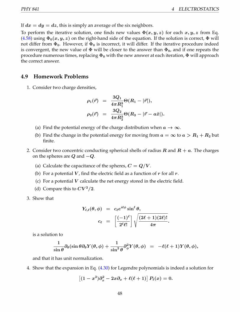
PHY 841 4 ELECTROSTATICS
If dx = dy = dz, this is simply an average of the six neighbors.
To perform the iterative solution, one finds new values Φ(x, y, z) for each x, y, z from Eq.(4.58) using Φ0(x, y, z) on the right-hand side of the equation. If the solution is correct, Φ willnot differ from Φ0. However, if Φ0 is incorrect, it will differ. If the iterative procedure indeedis convergent, the new value of Φ will be closer to the answer than Φ0, and if one repeats theprocedure numerous times, replacing Φ0 with the new answer at each iteration, Φ will approachthe correct answer.
4.9 Homework Problems
1. Consider two charge densities,
ρ1(r) =3Q1
4πR31
Θ(R1 − |r|),
ρ2(r) =3Q2
4πR32
Θ(R2 − |r − ax|).
(a) Find the potential energy of the charge distribution when a → ∞.
(b) Find the change in the potential energy for moving from a = ∞ to a > R1 +R2 butfinite.
2. Consider two concentric conducting spherical shells of radius R and R + a. The chargeson the spheres areQ and −Q.
(a) Calculate the capacitance of the spheres, C = Q/V .
(b) For a potential V , find the electric field as a function of r for all r.
(c) For a potential V calculate the net energy stored in the electric field.
(d) Compare this to CV 2/2.
3. Show that
Yℓ,ℓ(θ, ϕ) = cℓeiℓϕ sinℓ θ,
cℓ =
[(−1)ℓ
2ℓℓ!
]√(2ℓ+ 1)(2ℓ)!
4π.
is a solution to
1
sin θ∂θ(sin θ∂θY (θ, ϕ) +
1
sin2 θ∂2ϕY (θ, ϕ) = −ℓ(ℓ+ 1)Y (θ, ϕ),
and that it has unit normalization.
4. Show that the expansion in Eq. (4.30) for Legendre polynomials is indeed a solution for[(1 − x2)∂2
x − 2x∂x + ℓ(ℓ+ 1)]Pℓ(x) = 0.
48

PHY 841 4 ELECTROSTATICS
5. Show that the solution to Laplace’s equation in cylindrical coordinates when kz = 0,(∂2ρ +
1
ρ∂ρ
)R(ρ) −
m2
ρ2R(ρ) = 0,
becomes
Rm(ρ) =
Aρ−m +Bρm, m = 0,
C ln(ρ), m = 0.
6. Consider the function Φ = (x2 + y2) = r2 sin2 θ.
(a) Calculate ∇2Φ in Cartesian coordinates.
(b) Repeat in spherical coordinates
7. Consider a cavity that extends from x = −a to x = a and from y = 0 to y = ∞, i.e.it is infinite in the y direction. Assume it is infinite in both directions in the z direction.Along the y = 0 boundary, the surface is an insulator kept at a uniform potential V0,while the boundaries along the x = ±a surfaces are grounded. Note this means that atthe corner of the boundaries the potential is discontinuous, thus one might need to imaginean infinitesimal insulator at the intersection of the boundaries.
(a) Write down general solutions for the system that exponentially die for large y, andthat satisfy the B.C. that Φ(x = −a, y, z) = Φ(x = a, y, z) = 0. For the moment,ignore the B.C. at the y = 0 surface.
(b) Find the sum of such solutions from (a) that satisfies the B.C. that V (x, y = 0, z) =V0.
8. Consider the solution to a point charge outside a conducting sphere of radiusR performedwith images from the notes. Consider two point charges, one with charge Q at −az, anda second with charge −Q at az. As a → ∞, the sphere sees a constant electric field,E = 2Q/a2z. Find the electric potential from the two point charges and from the twoimages in the limit that a and Q both go to infinity in such a way that 2Q/a2 = E0.Compare your solution to that you get from using spherical harmonics.
9. Consider two infinite conducting planes at z = a and z = −a. A point charge Q isreplaced at the origin. Find a set of image charges that satisfy the B.C. for −a < z < a.
10. Using the solution for a conducting cylinder in a constant field from the notes, show thatthe electric field is perpendicular to the surface at ρ = R.
11. Consider a sphere of radiusR centered at the origin, The surface of the potential isV (cos θ).
(a) In spherical coordinates, using the azimuthal symmetry, the potential at r = R canbe written as
Φ(r = R, cos θ) =∑ℓ
aℓPℓ(cos θ).
Find Cℓ in the expression for aℓ of the form,
aℓ = Cℓ
∫ 1
−1
dx Φ(r = R, x)Pℓ(x).
49
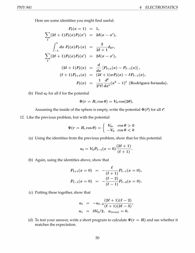
PHY 841 4 ELECTROSTATICS
Here are some identities you might find useful:
Pℓ(x = 1) = 1,∑ℓ
(2ℓ+ 1)Pℓ(x)Pℓ(x′) = 2δ(x− x′),∫ 1
−1
dx Pℓ(x)Pℓ′(x) =2
2ℓ+ 1δℓℓ′,∑
ℓ
(2ℓ+ 1)Pℓ(x)Pℓ(x′) = 2δ(x− x′),
(2ℓ+ 1)Pℓ(x) =d
dx[Pℓ+1(x) − Pℓ−1(x)] ,
(ℓ+ 1)Pℓ+1(x) = (2ℓ+ 1)xPℓ(x) − ℓPℓ−1(x),
Pℓ(x) =1
2ℓℓ!
dℓ
dxℓ(x2 − 1)ℓ (Rodriguez formula).
(b) Find aℓ for all ℓ for the potential
Φ(r = R, cos θ) = V0 cos(2θ).
Assuming the inside of the sphere is empty, write the potential Φ(r) for all r.
12. Like the previous problem, but with the potential
Φ(r = R, cos θ) =
V0, cos θ > 0−V0 cos θ < 0
(a) Using the identities from the previous problem, show that for this potential
aℓ = V0Pℓ−1(x = 0)(2ℓ+ 1)
(ℓ+ 1).
(b) Again, using the identities above, show that
Pℓ+1(x = 0) = −ℓ
(ℓ+ 1)Pℓ−1(x = 0),
Pℓ−1(x = 0) = −(ℓ− 2)
(ℓ− 1)Pℓ−3(x = 0).
(c) Putting these together, show that
aℓ = −aℓ−2
(2ℓ+ 1)(ℓ− 2)
(ℓ+ 1)(2ℓ− 3),
a1 = 3V0/2, a(even) = 0.
(d) To test your answer, write a short program to calculate Φ(r = R) and see whether itmatches the expectation.
50

PHY 841 5 MULTIPOLE EXPANSIONS
5 Multipole Expansions
Here, we consider fields due to compact figurations of static charges when viewed from faraway. The fields are dominated by the lowest non-zero moment of the charge distributions, e.g.monopole, dipole, quadrupole, etc.
5.1 Expanding Coulomb Potential in Spherical Harmonics
Consider a point charge Q at position az. We wish to express the Coulomb potential as anexpansion in 1/r, where if a = 0 only the first term survives.
Q
|r − az|=
Q√r2 − 2ar cos θ + a2
(5.1)
=Q
r
1√1 − 2(a/r) cos θ + (a/r)2
.
We now treat ϵ = 2(a/r) cos θ − (a/r)2 as a small number
Q
|r − az|=
Q
r
1√1 − ϵ
(5.2)
=Q
r
(1 + ϵ/2 + 3ϵ2/8 + 15ϵ3/48 · · ·
).
Organizing terms by powers of a/r,
Q
|r − az|=
Q
r
1 + (a/r) cos θ + (a/r)2
1
2(3 cos2 θ − 1) (5.3)
+(a/r)31
2(5 cos3 θ − 3 cos θ) + · · ·
.
One can see that this matches up with the expansion for the Legendre polynomials,
Q
|r − az|=
Q
r
∑ℓ
(a
r
)ℓ
Pℓ(cos θ). (5.4)
The above expression assumed the charge was along the z axis. One could prove this expressionterm-by-term, or simply apply the generating function for Legendre polynomials (copied fromEq. (4.34)),
1√1 − 2xt+ t2
=∑ℓ
Pℓ(x)tℓ. (5.5)
From one perspective, this generating function defines the Legendre polynomials, and otherproperties such as recurrence relations derive from the generating function.
51

PHY 841 5 MULTIPOLE EXPANSIONS
For our multipole expansion, we wish to find an expression for the field at some angle θ, ϕwhenthe charge is at angle θ′, ϕ′. The addition theorem for spherical harmonics,
Pℓ(cos γ) =4π
2ℓ+ 1
ℓ∑m=−ℓ
Y ∗ℓm(θ′, ϕ′)Yℓ,m(θ, ϕ), (5.6)
plays a critical role in going forward with the multipole expansion. The angle γ is the anglebetween the diretions θ, ϕ and θ′, ϕ′. Here is the proof, along with explanations of each step,(1)
(2)
(3)
(4)
(5)
(6)
(7)
(8)
Pℓ(cos γ) = Pℓ(cos γ)Pℓ(1) (5.7)
=4π
(2ℓ+ 1)Y ∗
ℓ0(0, 0)Yℓ0(γ, 0)
=4π
(2ℓ+ 1)⟨θ = 0, ϕ = 0|ℓ, 0⟩⟨ℓ, 0|γ, 0⟩
=4π
(2ℓ+ 1)
∑m
⟨θ = 0, ϕ = 0|ℓ,m⟩⟨ℓ,m|γ, 0⟩
=4π
(2ℓ+ 1)
∑m
⟨θ = 0, ϕ = 0|R−1R|ℓ,m⟩⟨ℓ,m|R−1R|γ, 0⟩
=4π
(2ℓ+ 1)
∑m
⟨θ = 0, ϕ = 0|R−1|ℓ,m⟩⟨ℓ,m|R|γ, 0⟩
=4π
(2ℓ+ 1)
∑m
⟨θ′, ϕ′|ℓ,m⟩⟨ℓ,m|ϕ, θ⟩
=4π
(2ℓ+ 1)
∑m
Y ∗ℓm(θ′, ϕ′)Yℓm(θ, ϕ). (5.8)
1. Use the fact that Pℓ(cos θ = 1) = 1.
2. Use the fact that Pℓ(cos θ) =√
4π/(2ℓ+ 1)Yℓ0(θ, ϕ).
3. Writing the Yℓm in bra-ket notation so that completeness is more apparent.
4. Yℓm(θ = 0) = 0 for all m = 0, so extra parts of sum can be added without changingresult.
5. R are rotations that move γ, 0 to θ, ϕ and 0, 0 to θ′, ϕ′.
6. Rotations don’t affect completeness |m⟩⟨m|.
7. Using definitions of rotation, note γ is angle between θ′, ϕ′ and θ, ϕ.
8. Leaving bra-ket notation.
The potential depends on the relative angle γ, so we can rewrite it as
Q
|r − a|=
4πQ
r
∑ℓm
1
(2ℓ+ 1)
(a
r
)ℓ
Y ∗ℓm(θ′, ϕ′)Yℓm(θ, ϕ), (5.9)
52
PHY 841 5 MULTIPOLE EXPANSIONS
where the potential is evaluated at r, θ, ϕ due to a charge at a, θ′, ϕ′.
Equation (5.9) has profound implications due to the fact that the same ℓm combination appearsin both spherical harmonics. If one expresses the angular distribution of the potential at somedistance r outside the charge distribution, the moments ℓ,m will depend only the moments ofthe local charge distribution with the same ℓ andm. To see this, we consider an array of charges,represented by a charge density ρ(r). Eq. (5.9) then gives
Φ(r) =4π
r
∫d3r′ ρ(r′)
∑ℓm
1
(2ℓ+ 1)
(r′
r
)ℓ
Y ∗ℓm(θ′, ϕ′)Yℓm(θ, ϕ), (5.10)
where θ, ϕ describe the direction of r and θ′, ϕ′ describe the direction of r′. For a fixed mag-nitude r, the θ, ϕ dependence of Φ(r) can be described by coefficients, Φℓm(r). Using thecompleteness relation for spherical harmonics,∫
dΩ Yℓ′m′(Ω)Yℓm(Ω) = δℓℓ′δmm′, (5.11)
one can see that the coefficients Φℓm can be consistently defined as
Φ(r, θ, ϕ) =∑ℓm
1
(2ℓ+ 1)Φℓm(r)Yℓm(θ, ϕ), (5.12)
Φℓm(r) = (2ℓ+ 1)
∫dΩ Y ∗
ℓ,m(θ, ϕ)Φ(r, θ, ϕ).
Thus, Eq. (5.9) becomes
Φℓm(r) =
∫dΩ Y ∗
ℓ,m(θ, ϕ)4π
r
∫d3r′ ρ(r′)
∑ℓ′m′
(r′
r
)ℓ′
Y ∗ℓ′m′(θ
′, ϕ′)Yℓ′m′(θ, ϕ) (5.13)
=4π
rℓ+1qℓm,
where qℓm are the multipole moments of the charge distribution,
qℓm =
∫d3r′ r′ℓρ(r′)Y ∗
ℓm(θ′, ϕ′). (5.14)
The potential can then be written as a sum over harmonic with coefficients given by qℓm,
Φ(r) =∑ℓm
4π
(2ℓ+ 1)qℓm
Yℓm(θ, ϕ)
rℓ+1. (5.15)
The moments, qℓm have dimension charge multiplied by length to the ℓth power, and the effectof higher moments falls off as 1/rℓ+1.
The lowest multipole moments can be re-expressed using the forms for the spherical harmonics
53

PHY 841 5 MULTIPOLE EXPANSIONS
in Eq.s (4.31),
q00 =1
√4π
∫d3r ρ(r) =
1√4πq, (5.16)
q11 = −√
3
8π
∫d3r ρ(r)(x− iy) = −
√3
8π(px − ipy),
q10 = −√
3
4π
∫d3r ρ(r)z = −
√3
4πpz,
q22 =
√15
32π
∫d3r ρ(r)(x− iy)2 =
√15
288π(Q11 − 2iQ12 −Q22),
q21 = −√
15
8π
∫d3r ρ(r)(x− iy)z = −
√15
72π(Q13 − iQ23),
q20 =
√5
16π
∫d3r ρ(r)(3z2 − r2) =
√5
16πQ33.
Here q is the net charge,
q =
∫d3r ρ(r), (5.17)
pi are the dipole moments,
pi =
∫d3r ρ(r)ri, (5.18)
andQij are the quadrupole moments,
Qij =
∫d3r ρ(r)(3rirj − r2δij). (5.19)
Example 5.1:Consider the charge density
ρ(r) = Axe−(x2+y2+z2)/2R2
.
Find all the multipole moments, qℓm for ℓ ≤ 2.Solution:First find the net charge q, the dipole moments pi and the quadrupole tensorQij . The net chargeq = 0 because the charge density is odd in x. Again, by symmetry, the only non-zero dipolemoment is px,
px = A
∫d3r x2e−(x2+y2+z2)/2R2
= (2πR2)3/2AR2.
The quadrupole tensor elements,Qij , are all zero because they all involve an overall even powerof coordinates. Some involve odd powers of x which would permit a non-zero result for the
54
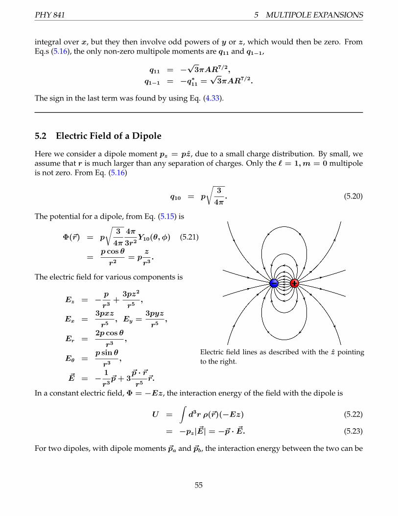
PHY 841 5 MULTIPOLE EXPANSIONS
integral over x, but they then involve odd powers of y or z, which would then be zero. FromEq.s (5.16), the only non-zero multipole moments are q11 and q1−1,
q11 = −√3πAR7/2,
q1−1 = −q∗11 =√3πAR7/2.
The sign in the last term was found by using Eq. (4.33).
5.2 Electric Field of a Dipole
Here we consider a dipole moment pz = pz, due to a small charge distribution. By small, weassume that r is much larger than any separation of charges. Only the ℓ = 1,m = 0 multipoleis not zero. From Eq. (5.16)
q10 = p
√3
4π. (5.20)
The potential for a dipole, from Eq. (5.15) is
Φ(r) = p
√3
4π
4π
3r2Y10(θ, ϕ) (5.21)
=p cos θ
r2= p
z
r3.
The electric field for various components is
Ez = −p
r3+
3pz2
r5,
Ex =3pxz
r5, Ey =
3pyz
r5,
Er =2p cos θ
r3,
Eθ =p sin θ
r3,
E = −1
r3p+ 3
p · rr5
r.
Electric field lines as described with the z pointingto the right.
In a constant electric field, Φ = −Ez, the interaction energy of the field with the dipole is
U =
∫d3r ρ(r)(−Ez) (5.22)
= −pz|E| = −p · E. (5.23)
For two dipoles, with dipole moments pa and pb, the interaction energy between the two can be
55

PHY 841 5 MULTIPOLE EXPANSIONS
found by considering the interaction energy of dipole b due to the field generated by dipole a,
U = −pb · Ea, (5.24)
Eb = −1
r3pb +
(pb · r)r5
r, r ≡ ra − rb,
U =pa · pbr3
−(pa · r)(pb · r)
r5.
In an extremely hot system, the average energy between two dipoles vanishes because on aver-age the directions of the dipoles are random and unaligned. However, if the system is at a finitetemperature T , a dipole moment is induced because the energy is lower if the dipole pointsparallel to the field. Finding the value of the average induced moment depends on how manyorientation states exist for the dipole, which is a matter for quantum mechanics. Classically, onewould average over all directions of the dipole,
⟨pz⟩ =
∫ 1
−1d cos θ p cos θepE cos θ/T∫ 1
−1d cos θ epE cos θ/T
(5.25)
=p
tanh(pE/T )−T
E.
For high temperatures, one can expand in pE/T and find
⟨pz⟩ =Ep2
3T.
The average interaction energy with an electric field is then
⟨U⟩ = −⟨p · E⟩ = −E2p2
3T, (5.26)
which is attractive. If the dipole in question, #1, is due to another dipole, #2, its interactionenergy depends only ⟨E2⟩ due to the dipole #2. If the two dipoles are separated by a distance r,and if the second dipole is basically randomly oriented (again, consistent with the high T limit),the average squared field is
⟨E2⟩ =1
2
∫ 1
−1
d cos θ[E2
r(r, θ) + E2θ(r, θ)
](5.27)
=p2
r6
∫ 1
0
d cos θ (4 cos2 θ + sin2 θ)
=2p2
r6.
The average interaction energy is then
⟨U⟩ = −4p4
3r6T. (5.28)
56

PHY 841 5 MULTIPOLE EXPANSIONS
An extra factor of two was added to account for the non-random part of the orientation of dipole#2 due to the random orientation with #1. This should be the dominant source of the potentialbetween two dipoles at large distances in the limit that the temperature is high enough that thedipoles are for the most part randomly distributed. At short distance, atoms or molecules beginto repel one another once the electronic wave functions attempt to overlap one another. Theseforces typically have forms that die off faster than 1/r6, perhaps exponentially or perhaps as ahigher power than 6. Indeed, the 1/r6 attractive force is known as the Van der Waals force andhas had great phenomenological success for a variety of phenomena. A common potential is the6-12 potential which behaves asA/r12 −B/r6.
5.3 Energy in arbitrary external field
As stated earlier, the energy of a charge in an external potential Φ, or that of a dipole in anexternal electric field is
U(monopole) = QΦ0, (5.29)
U(dipole) = −p · E0. (5.30)
The subscript “0” emphasizes that this is an external field, not the field from the charge or thedipole itself. This can be extended to arbitrary multipoles in an external field,
U =
∫d3r Φ(r)ρ(r), (5.31)
Φ(r) =∑
nxnynz
xnxynyznz
nx!ny!nz!∂nx
x ∂ny
y ∂nz
z Φ∣∣∣r=0
,
U =∑
nxnynz
1
nx!ny!nz!Mnxnynz ∂
nx
x ∂ny
y ∂nz
z Φ∣∣∣r=0
,
Mnxnynz =
∫d3r ρ(r)xnxynyznz .
The moments of the charge distribution,
M000 = q, (5.32)M100 = px,M010 = py,M001 = pz,
M200 = R11, M110 = R12, M101 = R13,
M110 = R21, M020 = R22, M011 = R23,
M101 = R31, M011 = R32, M002 = R33,
Rij ≡∫d3r ρ(r)rirj. (5.33)
57

PHY 841 5 MULTIPOLE EXPANSIONS
With these definitions,
U = qΦ0 − p · E0 −1
2Rij∂iE0j, (5.34)
= qΦ0 − p · E0 −1
6(Qij + Rδij)∂iE0j,
R ≡∫d3r r2ρ(r),
Qij ≡∫d3r (3rirj − r2δij)ρ(r).
where the fields and their derivatives are evaluated at r = 0. The term with R does not con-tribute to the energy because ∇ · E0 = 0 (the external field is that part of the field not affectedby local charge density), thus
U = qΦ0 − p · E0 −1
6Qij∂iE0j. (5.35)
Here, the quadrupole moment tensor Qij is defined as it was previously in this chapter, Eq.(5.19).
5.4 Homework Problems
1. Consider four charges +q,+q,−q,−q at the Cartesian positions (a, 0, 0), (0, a, 0), (−a, 0, 0),(0,−a, 0) respectively.
(a) Find the dipole moments pi and the quadrupole tensorQij for all i and j.
(b) Find all qℓm for all ℓ ≤ 2.
2. Consider a charge distribution with q21 = q2−1=some imaginary number iQa2, see defini-tions in Eq. (5.16). Draw a figure where you place a minimum number of discrete chargesthat reproduces the given q21 and q2−1, while having all other qij = 0 for ℓ ≤ 2.
(a) Provide the positions and find the individual charges, all of which are ±q, in terms ofQ. Only place charges on a lattice where the step size is a, i.e. at positions ia, ja, ka,where i, j, k are integers.
(b) In terms of the magnitude of the individual charges, q, and the lattice spacings a, findthe potential as a function of r, θ and ϕ.
3. Consider a simple model of an atom being a particle of charge e that moves in a three-dimensional harmonic oscillator with effective spring constant k. A constant electric fieldE0 is added.
(a) What is the magnitude of the induced dipole moment p?
(b) What is the change in total energy of the charge due to the introduction of the field?Give answer in terms of p and E0.
58

PHY 841 5 MULTIPOLE EXPANSIONS
4. Consider a point charge q at r′ = az.
(a) Find the moments, qℓm defined in Eq. (5.14), for all ℓ and m, defining the momentsaround the origin
(b) Show that the potential calculated with qℓm using Eq. (5.15) matches Eq. (5.9) for thecase where the charge is along the z axis.
(c) Show that for the case where Φ(r) is evaluated with r lying along the z-axis that thesum becomes q/(r − a).
5. Any function that can be written as a sum over Cartesian polynomials of order ≤ ℓ, i.e.,
F (x, y, z) =∑
ℓx+ℓy+ℓz≤ℓ
Aℓxℓyℓzxℓxyℓyzℓz ,
can be expressed as a sum of spherical harmonics with order ≤ ℓ,
F =∑
ℓ′,m′,ℓ′≤ℓ
Aℓ′m′(r)Yℓ′m′(θ, ϕ).
Using this fact prove that the multipole moments of order ≤ ℓ, for the case when all mo-ments qℓ′m′ vanish for ℓ′ < ℓ, are unaffected by a translation of the origin, and that thehigher moments, > ℓ, are affected by this change of the coordinate system. This meansthat the dominant multipole is unaffected by a translation of the coordinate system.Hint: Using the definition of the moments, Eq. (5.14), replace ρ(r) with ρ(r + a), thenexpress the new charge density as a Taylor expansion in powers of a.
59

PHY 841 6 MAGNETOSTATICS
6 Magnetostatics
Here, we consider magnetic fields from steady currents, and set the stage for fields from dynamicsources.
6.1 The Biot-Savart Law
In Chapter 2 we derived Maxwell’s equations from Lagrangians written in terms of the vectorpotential, and for electrostatics the Maxwell equation that was ∇2Φ = −∇ · E = −4πρ.This then led to Coulomb’s law. Here, we show one can similarly relate ∇2A = 4πJ , so thateach component of A is related to the corresponding component in J in the same manner thatΦ = A0 is related to ρ = J0.
To this we begin with the Maxwell relation in a static system (∂tE = 0),
∇ × ∇ × A = 4πJ, (6.1)∇2A− ∇(∇ · A) = −4πJ.
This last step is a simple vector identity, a× (b× c) = b(a · c)− (a · b)c, with a = b = ∇ andc = A.
Our difficulty going forward is the term ∇(∇ · A). However, one can eliminate that term bychoosing a convenient gauge. As show earlier, one can add a term to the vector potential, A′ =
A + ∇Λ, without changing any physics, because E and B are unchanged. This works for anyfunction Λ(x, y, z). We are in need of a new vector potential A′ where ∇ · A′ = 0,
∇ ·(A+ ∇Λ
)= 0, (6.2)
∇2Λ = −∇ · A.
If there were some charge density, ρ = ∇ · A, then finding Λ would be equivalent to findingthe potential corresponding to the static charge density. Of course, there is such a potential, thusthere is always a gauge such that ∇ · A = 0. Assuming one is in that gauge,
∇2A = −4πJ. (6.3)
Of course, due to gauge invariance there are many vector potentials one could choose, but theyall lead to the same electromagnetic fields. Thus, we are free to choose this gauge.
Equation (6.3) is actually three separate equations. Each one is effectively a Poisson’s equationwhere the components Ji play the role of charge densities. This is equivalent to Poisson’s equa-tion for the electric potential, ∇2Φ = −4πρ, so one can use the same results as before. Mainly,
A(r) =
∫d3r′ J(r′)
1
|r − r′|. (6.4)
60

PHY 841 6 MAGNETOSTATICS
The magnetic field is then
B(r) = ∇ × A (6.5)
=
∫d3r′
J(r′) × (r − r′)
|r − r′|3,
which is the Biot-Savart Law.
Note the expression assumes natural units, if the currents are in MKSA units, where Amperes(Coulombs/s) are the unit of current, the expression picks up an additional factor,
B(MKSA)(r) =µ0
4π
∫d3r′
J(r′) × (r − r′)
|r − r′|3, (6.6)
µ0 = 4π10−7 Tm/A.
Example 6.1:A 5 Ampere current travels through a thin wire in a circular loop of radiusR = 10 cm. Find thestrength of the magnetic field in the center of the loop.Solution:The current density element Jd3r′ becomes Idℓ for a thin wire. Each element Idℓ provides adifferential component to the magnetic field that is perpendicular to the plane of the loop (we’llcall it z). Integrating around the loop,
B(MKSA)(r = 0) =µ0I
4π
∫dℓ
z
R2, (6.7)
|B(MKSA)(r = 0)| =µ0I
2R= π · 10−5 T. (6.8)
6.2 Magnetic Moments
If one is outside a localized current distribution, the vector potential falls off according to thesame mathematics as used for multipole moments of the electric potential from the previouschapter. Because the net current density is zero for a confined static current,∫
d3r Ji(r) = 0, (6.9)
the “monopole” charge for each component i vanishes. Whereas p referred to the dipole momentof a charge distribution, here we will worry about equivalent of a dipole moment vector for eachcomponent Ji. Thus, we consider the moment
πij =
∫d3r′ Ji(r
′)r′j. (6.10)
61

PHY 841 6 MAGNETOSTATICS
Far away, the dipole contribution to the ith component of the vector potential is
Ai(r) =πijrj
r3, (6.11)
where we have simply translated from the result for the electric potential for a dipole, Φ =p · r/r3. Next, one can find the magnetic field,
Bi = ϵijk∂jAk (6.12)
= ϵijk
(πkj
r3− 3
πkℓrℓrj
r5
).
Using the identity,ϵijkϵkℓn = δiℓδjn − δinδjℓ, (6.13)
One can see that1
2ϵijkϵkℓnπℓn =
1
2(πij − πji) (6.14)
= πij,
where the last step used the fact that πij is anti-symmetric (which follows from current conser-vation, see end-of-chapter problem). Defining the magnetic moment m,
mi ≡ −1
2ϵijkπjk =
1
2ϵijkπkj, (6.15)
m =1
2
∫d3r r × J .
one can express πij in terms of m,
πij = −ϵijkmk. (6.16)
Inserting these into the expression for B in Eq. (6.12),
Bi =2mi
r3+
3
r5ϵijkϵkℓnmnrjrℓ (6.17)
=2mi
r3+
3
r5(δiℓδjn − δinδℓj)mnrjrℓ
= −mi
r3+
3ri
r5(m · r)
B = −m
r3+
3r
r5(m · r).
For a current loop with a thin wire, the magnetic moments have a simple geometric expression.For a thin wire one can
d3r = dℓd2r⊥, (6.18)
dℓ
∫d2r⊥J(r) = Idℓ,
m =1
2
∫dℓ r × I
=I
2
∫r × dℓ.
62

PHY 841 6 MAGNETOSTATICS
If the current lies in a plane, |m| = Ia, where a is the area of the loop, and the direction of m isperpendicular to the plane. Here, dℓ is along the direction of the wire and r⊥ is perpendicularto the wire.
6.3 Magnetic Forces and Torques
The magnetic force qv × B leads to torques on small current loops. In a magnetic field B, thenet force acting on some set of currents J is
F =
∫d3r J × B, (6.19)
because Jd3r is the differential contribution to qv. For a constant magnetic field B factors outfrom the integral and one can see that the net force acting on a static current distribution is zerobecause
∫d3r J = 0 (See end-of-chapter problem). Nonetheless, there is a net torque,
τ =
∫d3r′ r × (J(r′) × B), (6.20)
τi = Bk
∫d3r′ r′kJi(r
′) −Bi
∫d3r′ r′kJk(r
′).
Now one can use that fact that
πik ≡∫d3r′ r′iBk(r
′) (6.21)
is anti-symmetric to throw away the second term, and rewrite the first term,
τi =1
2Bk
∫d3r′
[r′kJi(r
′) − r′iJk(r′)]
(6.22)
τ =1
2
[∫d3r′ r′ × J(r′)
]× B
= m× B.
The work done by the torque in rotating an object is τdθ, so the potential energy of the dipole is
U = −m · B, (6.23)
and magnetic dipoles prefer to be aligned parallel to a magnetic field.
For two physically separated dipoles, ma and mb, one can then calculate the energy associatedwith their spin configuration using Eq. (6.17) which gives the magnetic field due to dipole a thatwould be experienced by dipole b,
U = −mb ·[−ma
r3+
3r
r5(ma · r)
](6.24)
=ma · mb
r3−
3r
r5(ma · r)(mb · r).
63

PHY 841 6 MAGNETOSTATICS
6.4 Overlapping Distributions and Hyperfine Splitting
Thus far, we have considered only the interaction between to distributions separated by a finiteamount. Sometimes, e.g. electrons interacting with a nucleus to produce the hyper-fine inter-action, the two distributions lay atop one another. Here, we consider the electric and magneticfield integrated over volumes that include all charges. This does not provide the entire distribu-tion of the field, but for energies such as −p · E or −m · B, it will give the interaction energiesfor a smooth distribution of electric or magnetic dipole densities within a volume. This mainlycomes into play in the interior of atoms. For examples, the smooth distribution of electron den-sity, and therefore the magnetic-dipole density, are well known from solving the Schrödingerequation. This interacts with the magnetic field due to the nuclear magnetic dipole. Because theelectron density is smooth, one needs only integrate the magnetic dipole density of the electronsmultiplied by the magnetic field due to the nuclear magnetic dipole.
To calculate the magnetic interaction of a nuclear magnetic moment, µN , with the intrinsic spinof electrons electrons in an atom, ρe, one would do the integral
U = −µe
∫d3r [ρe,↑ (r) − ρe,↓(r)] Bz(r), (6.25)
where Bz would be the field due to the nuclear magnetic moment. The magnetic moment of anelectron is
µe = geeℏ2me
, (6.26)
where ge ≈ 2.0 is the g−factor for electrons, and the ↑ and ↓ symbols denote the densities ofspin-up or spin-down electrons respectively. The difficulty with performing the integral in Eq.(6.25) is that we know how to calculate the magnetic field due to a magnetic moment at distancesoutside the nucleus, but within the current it is more difficulty. This is a small volume, but thefields are strong. Also due to the smallness, the density of electrons can be taken as constantwithin it, which means we need only the integrated value of Bz. The energy within this smallspherical volume of radius we denote as
UΩ ≈ −µe(ρe,↑ − ρe,↓)(r = 0)
∫r<R
d3r Bz(r). (6.27)
This approximation is excellent because the radius of a nucleus is ∼ 10−4 that of the electroncloud. Our goal is then to calculate
BV =
∫r<R
d3r B(r), (6.28)
due to the nuclear magnetic moment
µN = gNeℏ
2MN
z. (6.29)
We will consider both the cases of the electric and magnetic fields. First, we find an expressionfor EV and BV for the case where all charges and currents are within the volume, then move to
64

PHY 841 6 MAGNETOSTATICS
the case where all charges and currents are within the volume. The electric potential in a volumewith no charges can be expanded in spherical harmonics,
Φ(r) = Φ(r = 0) − E(r = 0) · r +∑
ℓ>2,m
AℓmYℓm(θ, ϕ)rℓ. (6.30)
Calculating the integrated electric field, only the ℓ = 1 term contributes and one finds,
EV = −∫r<R
d3r∇Φ (6.31)
=4πR3
3E(r = 0),
because all other terms will be constructed from Yℓ,ms with ℓ > 0 so they vanish. For example,if one applies the gradient operator, which transforms as an ℓ = 1 object, to rℓYℓ,m, the resultingpieces will consist of terms that behave as Yℓ−1,m′ and Yℓ+1,m, which will all integrate to zerofor ℓ ≥ 2. Thus, if there are no charges within a spherical volume, the integrated electric field isthe the electric field at the center multiplied by the volume. This means that the average electricfield within a spherical volume with no charges is the electric field at the center.
Similarly, one can do the same for the magnetic field. Again, one can make an expansion for thevector potential components in the Coulomb gauge, A, in spherical harmonics because ∇2A =0 in a region with no currents,
A(r) = A(r = 0) −1
2r × B(r = 0) +
∑ℓ>2,m
AℓmYℓm(θ, ϕ)rℓ. (6.32)
When calculating
BV =
∫r<R
d3r∇ × A (6.33)
=4πR3
3B(r = 0).
Thus the average magnetic field in a volume with no currents is the magnetic field at the center.
Next, we calcuate the average field in a spherical volume that contains all the charges or currents.First, we consider the electric field
EV =
∫r<R
d3r E(r) (6.34)
= −∫d3r∇Φ
= −R2
∫dΩ rΦ(R,Ω).
All the charges are inside R, so one can expand Φ in multipoles. Using the fact that the unitvector in the outward direction is
r = sin θ cosϕx+ sin θ sinϕy + cos θz, (6.35)
65

PHY 841 6 MAGNETOSTATICS
one can see that r only has ℓ = 1 terms of Φ contribute when the angular dependencies areexpressed in Yℓms. Thus, only the ℓ = 1 parts of Φ contribute, which are the dipole pieces.
EV = −R2
∫dΩ
p · rr3
r, (6.36)
EV,i = −R2
∫dΩ
pjrj
r3ri,
EV = −4π
3p.
To convince yourself the last step is correct, define the z axis to be along p, then only the z partof r contributes.
Next, one can calculate the corresponding quantity for magnetic fields. Similar as before,
BV =
∫r<R
d3r B(r) (6.37)
= ϵijk
∫d3r ∂jAk
= R2ϵijk
∫dΩ rjAk(R,Ω).
One can expand Ak in the same way Φ was expanded. Again, only the ℓ = 1 terms contribute.That term is given in Eq. (6.11),
BV = R2ϵijk
∫dΩ rj
πkℓrℓ
r3(6.38)
= −R2ϵijkϵkℓnmn
∫dΩ
rjrℓ
r4
= −4π
3ϵijkϵkjnmn
=8π
3mi,
BV =8π
3m.
Summarizing these results for the electric and magnetic fields,∫r<R
d3r E(r) =
−4πp/3, all charges within sphere
E(r = 0)V, all charges outside sphere(6.39)
E(r) ≈ Emultipole(r) −4π
3pδ3(r),∫
r<R
d3r B(r) =
8πm/3, all currents within sphere
B(r = 0)V, all currents outside sphere,
Here, V is the volume of the sphere. Putting these results together, we can express the magneticfield due to a magnetic moment as
B(r) ≈ Bmultipole(r) +8π
3mδ3(r). (6.40)
66

PHY 841 6 MAGNETOSTATICS
electron −2.00231930436182 ± 0.00000000000052muon −2.0023318418 ± 0.0000000013
proton 5.585694702 ± 0.000000017neutron −3.82608545 ± 0.00000090
Table 1: g factors for various particles. Even the neutral neutron has a magnetic moment because it isconstructed of charged up and down quarks.
These expressions assume the electric and magnetic dipoles are confined to a spatially small re-gion, with “small” being relative to the distributions with which they interact. The constructionclearly provides the correct field outside the volume of the dipole, and in the neighborhood ofthe dipole it integrates to the correct value. This is sufficient for the purposes of calculating thehyperfine interaction, between the magnetic field of the dipole and the smooth electron cloud.
The hyperfine interaction involves the coupling of the magnetic moments of the electron, mue
with the magnetic fields arising from the nuclear magnetic moment, µN .
U =(µN · µe)
r3−
3(µN · r)(µe · r)r5
−8π
3(µN · µe)δ
3(r) − e(µN · L)mr3
. (6.41)
The last term arises because if the electron is moving with finite angular momentum, it generatesa magnetic field which then couples with the nuclear magnetic moment. This term only comesinto play if the net orbital angular momentum of the electrons is non-zero.
Magnetic moments have dimensions of charge multiplied by velocity. For a classical particle ofcharge emoving in a circle of radiusRwith velocity v, the current and magnetic moment wouldbe
I =e
2πR/v, (6.42)
µ(class) =IR
2=ev
2
µ =eL
2m.
For intrinsic spin, S, this no longer holds, and we use a factor g to describe the ratio of µ to theclassical expectation,
µ = geS
2m= g
S
ℏ
(eℏ2m
). (6.43)
The last factor, eℏ/2m (or eℏ/2mc) depending on the units of magnetic field) is known as aBohr magneton. The g-factor is nearly 2.0 for point-particle fermions (e.g. electrons), differingfrom 2 due to higher-order perturbative corrections of order e2. Protons are not point particlesand the g-factor depends on details of the spin and angular momentum configuration of theconstituent quarks.
67

PHY 841 6 MAGNETOSTATICS
6.5 Homework Problems
1. Prove the following using current conservation (∇ · J = 0 for static systems):
(a) Beginning with ∫d3r (∇ · J(r))ri = 0,
show that ∫d3r Ji(r) = 0.
(b) Beginning with ∫d3r (∇ · J(r))rirj = 0,
show that πij is antisymmetric, where
πij ≡∫d3r Ji(r)rj.
2. Consider two current loops, each moving in the z = 0 plane. Each loop has current I andradius a. The first loop is centered at x = −a, y = 0 and is circulating clockwise, and thesecond loop is centered at x =, y = 0 and is circulating counter-clockwise.
(a) Calculate the analog of the quadrupole moment for calculating the ith component ofthe vector potential,
Qikℓ =
∫d3r Ji(r)(3rkrℓ − r2δkℓ).
(b) Find the vector potential Ai(r) far away, to order 1/r3. Use relations from the pre-vious chapter, where you merely add an additional index to account for the fact youare dealing with the vector potential. You can leave your answer in terms ofQikℓ, butclarify which components ofAi are zero, and how each component depends explicitlyon the angles θ and ϕ.
3. A particle of mass m and charge e moves in a circular orbit of radius R with angularmomentum L. What is the magnitude of the magnetic field at the origin? Note this wasused in writing the expression in Eq. (6.41) for the hyper-fine coupling.
4. Using Eq. (6.41), consider the hyper-fine energies for the 1s levels of a hydrogen atom.There are two levels because the electron and proton spin can couple to either zero orunity.
(a) Which terms in Eq. (6.41) contribute to the energy?
(b) Find the difference between the energy levels. Express your answer numerically ineV, using the electron mass and charge, and using the fact that the hydrogen atomelectron density for the 1s state behaves as
ρ(r) ∼ e−2r/a0,
a0 = 0.529 Å.
68

PHY 841 6 MAGNETOSTATICS
(c) What would the wavelength of light be for a transition between the states.
5. Consider a parallel-plate capacitor where the area of the plates is A and the small separa-tion is a. The charge on the plates are ±Q.
(a) What is the dipole moment of the capacitor if the plates are aligned in the z direction?
(b) What is the electric field in the capacitor?
(c) Determine whether Eq. (6.36) is satisfied in this case where the spherical volume en-gulfs the entire capacitor and one assumes the electric field is assigned to the interiorof the capacitor.
69

PHY 841 7 ELECTROMAGNETIC WAVES
7 Electromagnetic Waves
In the last several sections we have considered static systems, where we could neglect all the∂t · · · terms in Maxwell’s equations. In this chapter we consider the propagation of waves, andwave equations clearly require the ∂t.... terms.
7.1 The Wave Equation
Leaving off the current and charge density terms in Maxwell’s equations,
∇ · E = 0, (7.1)∇ · B = 0,
(∇ × B) − ∂tE = 0,
∂tB + ∇ × E = 0.
One can add the curl of the third equation to the time derivative of the fourth to obtain
∇ × (∇ × B) + ∂2t B = 0, (7.2)
−∇2B + ∇(∇ · B) + ∂2t B = 0,
∇2B = ∂2t B,
∂2B = 0.
This represents three separate wave equations, each with a wave velocity of unity. We wroteMaxwell’s equations in units where the speed of light is unity, otherwise the time derivativeswould change, ∂t → (1/c)∂t. Similarly, one can subtract the curl of the fourth equation abovefrom the time derivative of the second and obtain
∇2E = ∂2t E, (7.3)
∂2E = 0.
Equations (7.2) and (7.3) appear to represent six wave equations. For propagation along in thedirection of a wavenumber k axis, the solutions have the forms
Ei(r, t) = aieik·r−iωt, (7.4)
Bi(r, t) = bieik·r−iωt,
ω = |k|.
To discern the direction of propagation, one can ask for what δr would one considers a wavepacket with combinations of different wave numbers centered around k. The peak of the packetis defined by that point in coordinate space where the various wave numbers contribute with a
70

PHY 841 7 ELECTROMAGNETIC WAVES
steady phase, i.e.
∂ki
(ik · r − iω(k)t
)= 0, (7.5)
ri −∂ω(k)
∂kit = 0,
ri =k
|k|t.
The last step made use of the fact that ω = |k|. If one were in a medium, the group velocity,dω/dk, could differ from the speed of light, a subject for the next course.
The six solutions in Eq. (7.4) are not independent. In order to satisfy the connection between Eand B in Maxwell’s equations in Eq.s (7.1), once given E, one can find B, and vice versa. Also,in order to satisfy ∇ · E = 0 and ∇ · B = 0, the wave equations must satisfy
a · k = 0, (7.6)b · k = 0.
Thus, the six solutions for a given wave number become two. The amplitudes a and b must benormal to the wave number k and additionally, the third and fourth Maxwell’s equations requirethat
k × a = ωb, (7.7)k × b = −ωa.
There are two independent components of a given k. This defines the polarization. Once givena, b is also determined. The vector bwill be normal to both a and k. A solution with ax = 0 anday = 0 is considered linearly polarized in the x direction, whereas the solutions with ax = 0is linearly polarized in the y direction. One can consider ay = iax and find a solution wherethe real part of Ex is a cosine wave and the real part of Ey is a sine wave. These are circularlypolarized solutions.
7.2 Stress-Energy Tensor of Electromagnetic Waves
The zero-zero component of the stress-energy tensor is the energy density. Using the solutionsfor the waves in Eq. (7.4) and the stress-energy tensor for the electromagnetic field from Eq.
71

PHY 841 7 ELECTROMAGNETIC WAVES
(3.33),
T00 =1
8π
(|E|2 + |B|2
)(7.8)
=a2i + b2i8π
=|a|2
4πcos2(k · r − ωt),
T0i = ϵijkEjBk
4π
= ki|a|2
4πcos2(k · r − ωt),
T ij = −T ij =
1
8π(δij(E
2 +B2) − 2EiEj − 2BiBj)
=1
4π
|a|2δij − aiaj − bibj
cos2(k · r − ωt).
The factors cos2(k · r − ωt) arise from using only the real part of ei(k·r−ωt) and assuming a isreal (equivalent to saying the polarization is linear). Otherwise, phases, e.g. cos(k · r−ωt+ϕ)would enter.
For a wave moving along the z axis, with polarization components ax and ay,
T 00 =a2x + a2
y
4πcos2(kz − ωt), (7.9)
T 0z =a2x + a2
y
4πcos2(kz − ωt) = T 00,
T zz =a2x + a2
y
4πcos2(kz − ωt) = T 00,
T xx = T yy = T i =j = 0.
For the last expression, we used the fact that bx = −ay and by = ax, which comes fromEq. (7.7). These results are expected because T0z is both the momentum density and the fluxof energy. The energy flux is energy density multiplied by velocity, so one expects it to equalT00 because the velocity in unity. Further, Tzz is the flux of momentum, momentum densitymultiplied by velocity, so it equal to T0z = T00.
7.3 The Doppler Effect
An observer sees light from a source with wave number k. Its frequency is |k|. If the sourceis moving with velocity v, one can find the frequency of the emission according to an observermoving with the source, ωs, by treating the frequency and wave number as as four vector,
k = (ω, k). (7.10)
The frequency in the source frame is then found by the Lorentz transformation,
ωs = γ(ω − v · k) = ωγ(1 − v cos θ), (7.11)
72

PHY 841 7 ELECTROMAGNETIC WAVES
where θ is the angle between v and k. If the source is moving directly toward the observer,
ωs = ω
√1 − v
1 + v. (7.12)
If the source is moving away from the observer, the sign of v shifts, and the observed frequencyis less than the source frequency (red shift). If the source were to move perpendicular to theobserver, one would see the frequency shift by a factor γ, i.e. the red shift would be smaller butwould not vanish.
7.4 Wave Guides and Cavities
Here we consider oscillating solutions at fixed frequency. We consider the simplest case, that ofa vacuum surrounded by a perfect conductor. For non-perfect conductors the boundary condi-tions are more complicated due to the penetration of the fields into the media. Such penetrationalso leads to damping of waves. Because this course explicitly ignores electromagnetism in me-dia, our coverage of wave guides will be brief.
The boundary conditions for an electric field at a conductor are simple, E × n = 0 at thesurface. Any non-zero transverse field would cause an infinite current along the surface. Theconductor has no problem with the perpendicular component being non-zero. From Gauss’slaw, one can see that the surface charge density, σ = E · n/4π, can maintain the field beingzero inside the conductor. For waves the fields are changing in time, and Maxwell’s equation∇ × B = ∂tE demands that the presence of an oscillating electric field be accompanied byan oscillating magnetic field. Also, any oscillating magnetic field would be accompanied byan electric field due to the Maxwell’s equation, ∇ × E = −∂tB. This leads to the demand theB = 0 inside the conductor – except for static fields, which are not relevant for waves. Whereas acharge density can screen the perpendicular component of E, there is no such thing as magneticcharge density, ∇ · B = 0, so the boundary condition for magnetic field is B · n = 0. Onecan then consider the transverse magnetic field at the surface. One can draw a loop drawn justoutside the surface for a distance L, then cuts into the surface, return in the opposite direction−L inside the surface, then close the loop. If there is magnetic field along L outside the loop,one can still have no magnetic field inside the conductor if there is a surface current js. Thus,the boundary conditions for a perfect conductor are:
n× E = 0, (7.13)n · B = 0,
n · E = 4πσ,
n× B = 4πjs.
First we consider a rectangular wave guide, constrained in the x and y directions
0 < x < Lx, (7.14)0 < y < Ly.
73

PHY 841 7 ELECTROMAGNETIC WAVES
The equations of motion for a wave, rewriting Eq.s (7.2) and (7.3),
∇2E = ∂2t E, (7.15)
∇2B = ∂2t B,
and viewing the boundary conditions suggest solutions of the form for the electric field,
Ex(r, t) = E0xe−iωt+ikzz cos(qxx) sin(qyy), (7.16)
Ey(r, t) = E0ye−iωt+ikzz cos(qyy) sin(qxx),
Ez(r, t) = E0ze−iωt+ikzz sin(qyy) sin(qxx).
with
ω2 = q2x + q2y + k2z,
qx =nxπ
Lx
, qy =nyπ
Ly
,
nx and ny being any four integers. In principal, one could have imagined using different num-bers ni for Ex, Ey and Ez if they somehow added up to the same frequency due to a fortuitouschoice of Lx and Ly – we return to that further below. One can also write down solutions for themagnetic field wave equations,
Bx(r, t) = B0xe−iωt+ikzz sin(qxx) cos(qyy), (7.17)
By(r, t) = B0ye−iωt+ikzz sin(qyy) cos(qxx),
Bz(r, t) = B0ze−iωt+ikzz cos(qyy) cos(qxx).
By inspection one can see that these six components listed above have the same frequency andsatisfy the boundary conditions independently, i.e. any choice of the six amplitudesE0i andB0i
would work. However, one must also satisfy the Maxwell’s equations that link E and B,
∂tB = −∇ × E, (7.18)∂tE = ∇ × B.
This leads to the conditions
−iωB0x = ikzE0y + qyE0z, (7.19)−iωB0y = −ikzE0x − qxE0z,
−iωB0z = qxE0y − qyE0x,
iωE0x = ikzB0y + qyB0z,
iωE0y = −ikzB0x − qxB0z,
iωE0z = qxB0y − qyB0x.
It might seem worrisome that we have six unknown amplitudes and six conditions, as we cer-tainly expect more than one solution, not to mention an arbitary multiplicative constant. How-ever, these conditions are not independent.
74

PHY 841 7 ELECTROMAGNETIC WAVES
In fact, there are two independent sets of solutions, each with an arbitrary overall amplitude.The first set of solutions is referred to as transverse magnetic (TM) and the second as transverseelectric (TE). For TM solutions, we setB0z = 0 and for TE solutions we setE0z = 0. For the TMcase, we solve for the remaining amplitudes in terms of E0z. The algebra gives
E0x = −iqxkz
ω2 − k2z
E0z, (7.20)
E0y = −iqykz
ω2 − k2z
E0z,
B0x = −ikz
ω
qykz
ω2 − k2z
E0z − iqy
ωE0z,
B0y = ikz
ω
qxkz
ω2 − k2z
E0z + iqx
ωE0z.
Similarly, one can solve for TE amplitudes in terms ofB0z,
E0x = −ikz
ω
qykz
ω2 − k2z
B0z − iqy
ωB0z, (7.21)
E0y = ikz
ω
qxkz
ω2 − k2z
B0z + iqx
ωB0z,
B0x = −iqxkz
ω2 − k2z
B0z,
B0y = −iqykz
ω2 − k2z
B0z.
The group velocity is not the speed of light. From the dispersion relation (ω vs kz) one can findthe group velocity,
ω2 = k2z + q2x + q2y, (7.22)
vg =dω
dkz=kz
ω=
kz√k2z + q2x + q2y
.
The group velocity is less than the speed of light, and takes the form of a massive particle withm =
√q2x + q2y.
The procedure can be followed for any cross-sectional shape, assuming the wave-guide is trans-lationally invariant along the z axis. One can always divide the solutions into TM and TE modes.For the TM modes, one can solve the boundary conditions first for the function ψ(x, y), whichgives Ez(x, y) by the relation,
Ez = ψ(x, y)e−iωt+ikzz. (7.23)
One can solve the equations for ψ from the differential equation,
−(∂2x + ∂2
y)ψ = −(ω2 − k2z)ψ, (7.24)
75

PHY 841 7 ELECTROMAGNETIC WAVES
with the boundary conditions
ψ(x, y)|S = 0. (7.25)
This boundary condition forces Ez to be zero at the surface. Once one has solved the boundarycondition, the transverse components of the electric and magnetic fields can be found via,
Et(x, y) =ikz
(ω2 − k2z)e−iωt+ikzz∇tψ(x, y), (7.26)
Bt(x, y) =
(ω
kz
)z × Et.
The expression for Et manifestly points into the surface because ψ is constant along the surface.Then, Bt, which is normal to both Et and z must lie parallel to the surface. Our next task is toshow that these expressions solve each of the four Maxwell’s equations. For example,
∇ × B =? ∂tE, (7.27)(ω
kz
)∇ × (z × Et) =? −iω
(Et + ψe−iωt+ikzzz
), (7.28)
1
kzz(∇ · Et) −
1
kz∂zEt =? −i
(Et + ψe−iωt+ikzzz
), (7.29)
∇2tψ
(ω2 − k2z)
=? −ψ. (7.30)
One can check the other Maxwell equations (See HW problems).
For TE modes, a similar procedure can be applied. In that case
Bz = ψ(x, y)e−iωt+ikzz, (7.31)
with ψ(x, y) still satisfying Eq. (7.24), but with the boundary conditions
(n · ∇t)ψ(x, y)|S = 0. (7.32)
The transverse fields are then given by,
Bt(x, y) =ikz
(ω2 − k2z)e−iωt+ikzz∇tψ(x, y), (7.33)
Et(x, y) = −(ω
kz
)z × Bt.
7.5 Homework Problems
1. Consider the Lagrangian density
L =1
4F µνFνµ −
λ
2(∂ ·A)2.
Here, the action is S = (1/4π)∫d4x L. The extra term here (proportional to λ) is known
as the gauge-fixing term, which is a misnomer. This term explicitly destroys gauge invari-ance, so after one calculates quantities, one must actually use the Lorentz gauge, ∇·A = 0to recover the correct result.
76

PHY 841 7 ELECTROMAGNETIC WAVES
(a) Consider the Feynmann gauge (not actually a gauge, but just a choice for λ), whereλ = 1. Show that the Lagrangian, after integrating the action by parts, becomes
L = −1
2∂αAβ∂αAβ.
(b) Solve for the equations of motion in the Feynmann gauge. Then, setting ∂·A = 0, andusing Eq.s (2.40), show that the equations of motion become the Maxwell’s equationsfor free space,
∇ · E = 0, (7.34)∇ × B = −∂tE.
(c) (Extra Brownie Points) Write down the stress-energy tensor in the Feynmann gauge.Then, set ∂ · A = 0, show that T00 = (|E|2 + |B|2)/2. You may also need to applyequations of motion and use some messy vector identities.
2. Consider solutions for electro magnetic waves of frequency ω moving in the ±z directionswhich are linearly polarized in the x direction. Assume the incoming wave has a formE0xe
−iωt+ikz/2.
(a) Find the linear combination of such waves where the electric field vanishes at z = 0,i.e. reflecting off a conducting plane. Express your answer for both E and B as a realfield in terms of sines and cosines.
(b) Find the elements of the stress-energy tensor as a function of z and t.
(c) Show that the stress-energy tensor is traceless, T ii = 0.
3. Consider a plane wave moving in the z direction according to Eq. (7.4) with ay = iax andax real. Taking the real part of the solution, solve for the direction of a as a function of timeand position.
4. Consider a simple model of the universe where the expansion velocity for cosmologicalpurposes is v = r/t. This corresponds to a “flat” universe with gravitational effects ig-nored. All matter starts at a point (the origin) and there is no acceleration for any fluidelement. Observer A is moving with the source, and she records light being emitted at atime τ0 = 105 years after the birth of the universe, according to a clock in her pocket. Asecond observer, B, records the light moving past at a time τ = 1.4 × 10¹⁴ years afterthe beginning of the universe according to a watch in his pocket. Both A and B are at restrelative to the neighboring expanding matter. If observer A records the frequency of theemitted light as being f0, find the frequency f of the recorded light according to observerB.Some Help: the time measured by the co-moving observer, τ , is related to the time mea-sured by a different observer with velocity v by the relations:
τ =t
γ= t
√1 − v2 = t
√1 − r2/t2 =
√t2 − r2.
77

PHY 841 7 ELECTROMAGNETIC WAVES
5. Show that there is no solution to the conditions for the rectangular wave-guide amplitudesin Eq. (7.19) when both E0z and B0z are set to zero. This demonstrates that there are nosolutions other than the TE and TM solutions.
6. Show that Eq.s (7.23-7.26) satisfy the Maxwell relation ∇ × E = −∂tB.
7. Consider a cylindrical wave-guide of radiusR. Consider the lowest frequency TM solutionto the generating function ψ satisfying the differential equation
∇2tψ(ρ, ϕ) = −α2ψ(ρ, ϕ), α2 = ω2 − k2
z,
where kz is the wavenumber for longitudinal motion.
(a) Find a solution for ψ in polar coordinates. Express answer in terms of a0, the firstzero of the Bessel function J0.
(b) Find expressions for the electric and magnetic fields.
(c) What is the group velocity of a wave with momentum kz.
8. Consider two infinite parallel plates with the plane of the plates being along the x directionand the separation being Lx, i.e. a rectangular wave guide with Ly = ∞. Consider awave moving in the z direction with wave number kz. Using the method of generatingfunctions,
(a) Solve for the lowest frequency TM wave. Find expressions for the fields and the groupvelocity.
(b) Solve for the lowest frequency TE wave. Again find expressions for the fields and thegroup velocity.
78

PHY 841 8 RADIATION
8 Radiation
Here we discuss classical radiation. The source of such radiation is the J · A terms in the La-grangian, and the “classical” assumption is that the current does not change due to the radiatedphoton. In contrast, quantum emission involves changing discrete levels. For instance one couldfall from a p-state to an s-state, with the frequency determined by the change in energy levels.For classical emission the frequency is a property of how charge moves within the source, and itis assumed that there is no feedback from the radiation that alters the current. Additionally, theclassical assumption ignores the fact that light of a given frequency carries quantized amount ofenergy, but this latter part of the assumption is irrelevant if one records many photons.
8.1 Coupling the Electromagnetic Field to Dynamic Currents and Charges
To incorporate dynamics into the generation of electric and magnetic fields, we consider Maxwell’sequations for electric and magnetic fields, written in term of the four-vector potentialAµ,
∂αFαβ = 4πJβ, (8.1)
∂α(∂αAβ − ∂βAα) = 4πJβ,
∂2Aβ − ∂β(∂ ·A) = 4πJβ.
Similar as to our derivations for magneto-statics, this last expressions could be treated as fourseparate Poisson’s equations if the second term of the bottom expression would disappear.Again, we argue that this term can be ignored because one can choose a gauge that explicitlycancels it, and given that physical results cannot depend on the gauge, that term cannot matter.The choice of Λ,
Aα(new) = Aα
(old) + ∂αΛ, (8.2)
must be able to enforce ∂ ·A(new) = 0.
∂ ·A(new) = ∂ ·A(old) + ∂2Λ = 0, (8.3)∂2Λ = −∂ ·A(old).
Just as before, for any scalar function ∇·A(old), one can find a solution to Poisson’s equation forΛ where ∂ · A(old) serves as a source. Physics doesn’t depend on Λ, so we choose Λ to satisfythe gauge constraint, and are thus left with simpler equations. This is know as the Lorentzgauge, and aside from being convenient, has an attractiveness due to its invariance to boosts orrotations,
∂ ·A = 0. (8.4)
We are thus left with four independent equations,
∂2Aα = 4πJα. (8.5)
When the right-hand side was set to zero this is known as Laplace’s equation, when the right-hand side is non-zero, and independent of A, it is Poisson’s equation. The right-hand side can
79

PHY 841 8 RADIATION
be thought of as a source term. If there are no fields at t → −∞, any subsequent appearanceof fields is due to the source term. The equation is linear in A, so one can write the solutions asa sum (integral) over solutions from each differential contribution on the right-hand side. If theright-hand side were,
∂2G(x) = δ4(x), (8.6)
and if the solutionG> satisfied the boundary conditions of being zero for all negative times, onecan apply this solution to write solutions for any form on the right-hand side. For an arbitrarysource function, S(x), where one is searching for a solution F (x),
∂2F (x) = S(x), (8.7)
one could write the solution for F as
F (x) =
∫x′0<x0
d4x′ S(x′)GR(x− x′), (8.8)
which effectively is taking a linear combination of solutions for each differential source elementto generate a solution for a continuous source. For the case here, the source function for solvingfor the evolution ofAα(r) is 4πJα(r′), and
Aα(x) = 4π
∫x′0<x0
d4x′ Jα(x′)GR(x− x′). (8.9)
The function GR(r), the retarded Green’s Function, is independent of the source, and appliesto any Poisson equation. The retarded solution is the solution to the differential equation in Eq.(8.6) that vanishes for negative times.
The Green’s function is found by solving Eq. (8.6). By inspection, one can see that
G(t, r) =−1
(2π)4
∫dωd3k
eiωt−ik·r
ω2 − k2(8.10)
is a solution to Eq. (8.6). However, this solution does not satisfy the boundary conditions that itvanish for all negative times. Altering the solution to satisfy the boundary condition,
GR(t, r) =−1
(2π)4
∫dωd3k
eiωt−ik·r
(ω − k − iϵ)(ω + k − iϵ), ϵ → 0 + . (8.11)
Performing the integral over ω by contour integration,
GR(t, r) =−i
(2π)3
∫d3k
1
2k
(eikt−ik·r − e−ikt−ik·r
)Θ(t) (8.12)
=1
(2π)3
∫d3k
1
ksin(kt)e−ik·rΘ(t).
Next, choosing θ as the angle between r and k, writing eik·r = eikr cos θ, and integrating overcos θ then k,
GR(t, r) =1
4π2r
∫ ∞
−∞dk sin(kt) sin(kr)Θ(t) (8.13)
=1
4πrδ(t− r).
80

PHY 841 8 RADIATION
This allows the vector potential to be written in terms of an integral driven by currents at previ-ous times,
Aα(x) =
∫d4x′ 1
|x− x′|Jα(x′)δ(x0 − x′
0 − |x− x′|). (8.14)
The physical interpretation of this is clear, the vector potential is driven by the configuration ofthe currents along the light-front. For the static case, Jα does not depend on time, one quicklyrecovers the usual expressions given in the previous sections (See HW problem).
8.2 Radiation from an Accelerating Point Charge
Radiative energy flux is given by the Poynting vector, S = E × B/4π, and because for staticcases E and B fall off at least as quickly as 1/r2, the flux must fall off faster than 1/r2 and thusthere is no radiated energy. However, this changes for the case of accelerated charges becausethe current density depends on time. . We consider the equation for vector potential, Eq. (8.14),and consider a moving point charge of charge e. In that case,
d4x′Jα(x′) = euαdτ, (8.15)
when the differential covers the particle’s position. Here, dτ is the differential time as measuredin the frame of the charge. To verify this, consider the frame of the particle, u = (1, 0, 0, 0). Inthat frame J0d3x = e, Jd3x = 0, which is the correct answer, and because the Lorentz indicesmatch, d4x is a scalar, it must be correct in all frames.
The vector potential is then
Aα(x) = 2e
∫dτ uα(τ )δ[(x− r(τ ))2]Θ(x0 − r0), (8.16)
where rα(τ ) is the trajectory of the particle. The extra factor of 2 and stepfunction, and themissing 1/| x− r| arise from the fact that the delta function is now a function of the invariantdistance squared. Given that (d/dx)δ(f(x)) = δ(f(x))/f ′, the expressions are equivalent.Because the new delta function would also contribute when r0 > x0, the step function is added.To find the electro-magnetic fields,
∂αAβ = 2e
∫dτ uβ∂αδ[(x− r(τ ))2] (8.17)
= 2e
∫dτ uβ
∂δ[(x− r(τ ))2]
∂τ
∂τ
∂(x− r(τ ))2∂α(x− r(τ ))2
= −2e
∫dτuβ
(x− r)α
(r − x) · u∂δ[(x− r(τ ))2]
∂τ
= 2e
∫dτ δ[(x− r(τ ))2]∂τ
uβ(τ )(r(τ ) − x)α
u(τ ) · (r(τ ) − x)
.
Here, we have made use of the fact that uα = drα/dτ . We are only interested in the fieldsfar away, x0 ≈ |x| >> ri. Thus, we need only worry about derivatives of u above because
81

PHY 841 8 RADIATION
derivatives of xwould result in additional factors of 1/x. Taking the derivatives, then throwingaway all terms that fall off too quickly,
∂αAβ(x) ≈ 2e
∫dτ δ[(x− r(τ ))2]
xαaβ
(u · x)aβ −
xαuβ
(u · x)2(a · x)
, (8.18)
aβ ≡d
dτuβ.
The zeroth component a can be rewritten (see HW problem) as a0 = u · a/u0. One can nowagain use the chain rule for delta functions to obtain
∂αAβ(x) =e
(u · x)2xα
(aβ −
uβ(a · x)(u · x)
). (8.19)
We are interested in radiation, which implies the long-distance limit where x → ∞, so wereplaced the ≈ sign in Eq. (8.18) with an equal sign and replaced u · (x− r) with u · x.
The electric and magnetic fields can now be calculated,
Ei =e
(u · x)2
x0
(ai −
ui(a · x)(u · x)
)− xi
(a0 −
u0(a · x)(u · x)
). (8.20)
With a significant amount of algebraic effort, one can express this in the form,
E = e
n× [(n− β) × ˙β]
(1 − β · n)3|x|
. (8.21)
Here, n is a unit vector in the direction of x, and β = u/u0 = v/c is the non-relativistic velocity.Again, with a bit of effort, one can see that the magnetic field is given by
B = n× E. (8.22)
The direction of E defines the polarization. For small velocities that direction can be found by
taking the direction of ˙β, then projecting out the part of the vector along x. The small velocity
limit, β << 1, also makes it easy to calculate the net power. The power per area is given by themagnitude of the Poynting vector. For β << 1,
|S| =1
4π|E|2 (8.23)
=e2
4π|x|2| ˙β|2 sin2 θ,
where θ is the angle between n and β. Integrating over the area, dA = 2π|x|2d cos θ, the netpower is
P =2e2
3c| ˙β|2, (8.24)
82

PHY 841 8 RADIATION
which is known as Larmor’s formula. The factor 1/cwas added should you need to calculate inunits where c = 1.
For relativistic motion, the expression is more complicated. In Eq. (8.21) one cannot ignore theβ in the numerator, but more dramatically, the denominator,
1
(1 − β · n)3, (8.25)
diverges as β → 1 when the emission direction x is parallel to the velocity β. This is especiallytrue for circular motion of electrons in a high energy accelerator. Due to their light mass β isvery nearly unity. The acceleration is inward, toward the center of the motion, so one can useEq. (8.21) to see that the emitted light is linearly polarized with E perpendicular to both theacceleration and the direction of the light, which tends to be parallel to the velocity. Thus, thatlight is polarized perpendicular to the plane of the motion.
8.3 Liénard-Wiechert Potentials
The expressions for the fields due to currents in the previous section assumed that the observerwas far away, in both distance and time, from the fields. A more general expression for thevector potential was given in Eq. (8.16),
Aα(x) = 2e
∫dτ uα(τ )δ[(x− r(τ ))2]Θ(x0 − r0), (8.26)
=euα(τ )
u · (x− r(τ )).
Here r(τ ) is the position of the particle at a time when a light-pulse from the particle’s trajectorywould reach space-time point x. Effectively, one would follow the trajectory until one foundsuch a point. Because the particle moves slower than the speed of light, there can be only onesuch point. The factor 1/(u · (x− r)) can be factored into
u · (x− r) = u0(x0 − r0) (1 − n · v) , (8.27)
Aα(x) =e(uα(τ )/u0)
1 − n · v,
where n is the unit vector parallel to x− r. As was seen in the last section, in the non-relativisticlimit this factor simply provides the inverse distance from the point of emission to the observer.However, relativistically the additional factor (1−n·v)−1 amplifies the response of the potentialto the charge when the velocity approaches the speed of light and is pointed toward the observer.
In a simulation of relativistic charged particles interacting electromagnetically, Liénard-Wiechertpotentials offer one way (probably not the most computationally efficient way) of including re-tardation effects. Rather than assuming instantaneous interactions, where the potentials dependon the current positions and currents of the particles, one would calculate the contribution to theAα(x) for some point x by using the positions and velocities of each charge at the appropriateretarded time.
83

PHY 841 8 RADIATION
8.4 Radiation from relativistic particles
The velocity of a proton in the LHC is 99.9999991% the speed of light. Electrons are lighter, soeven though the energy of the LEP ring of the LHC is smaller than that of the LHC, the speed ofan electron in LEP is 99.9999999988% the speed of light. In such cases the relativistic factors aresurprisingly large and non-trivial.
Using the results of Eq.s (8.21) and (8.22), the power per solid angle from an accelerating chargeis
dP
dΩ=
e2
4π(1 − β · n)6|(n− β) × ˙
β)|2. (8.28)
This represents the energy emitted into the solid angle during a time dx0. During that timeinterval dx0, the time interval of the particle’s trajectory that contributed to the emission is
dr0 = dx0
dr0
dx0
, (8.29)
(r − x)2 = 0,
2(r0 − x0)(dr0 − dx0) − 2(r − x) · dr = 0,
dr0
[r0 − x0 − β · (r − x)
]= dx0(r0 − x0),
dr0
dx0
=1
(1 − β · n).
The energy emitted per time interval of the accelerated charge is thus
dP
dΩ=
e2
4π(1 − β · n)5|n× [(n− β) × ˙
β)]|2. (8.30)
Here, θ is the angle between β and n. With a devoted effort, one can integrate the differentialexpression for power. The result for the remarkably difficult integral is
P =2
3ce2γ6
[β2 − |β × ˙
β|2]. (8.31)
According to Jackson, this is the Liénard result from 1898, which is remarkable given that specialrelativity was not generally explained until 1905.
First, we consider the case where β and ˙β are parallel or anti-parallel. This would be the case for
a linear accelerator or for a charge gradually stopping. In that case
dP
dΩ=
e2
4π(1 − β cos θ)5| ˙β|2 sin2 θ. (8.32)
The unusual angular shape is solely determined by the magnitude of the velocity β. It vanishesin the forward direction due to the sin2 θ factor, then has a maxima at an angle θmax < π/2. Inthe β << 1 limit, the maximum θmax ≈ π/2, and in the ultra-relativistic limit the maximumθmax ≈ 0 and the emission is strongly forward-peaked. The angular shape is identical for
84

PHY 841 8 RADIATION
-1.0 -0.8 -0.6 -0.4 -0.2 -0.0 0.2 0.4 0.6 0.8 1.0
cosθ
010
42×1
043×1
04
sin
2θ/
(1−
cosθ
)5
β=0.95
β=0.7(×200)
β=0.3(×1000)
Figure 8.1: The angular dependence from Eq. (8.32) is shown for three velocities. As β approaches thespeed of light, the strength of the radiation increases dramatically and the emission becomes stronglyforward-peaked. For the same acceleration, radiation increases by more than three orders of magnitudeas β increases from 0.5 to 0.95.
accelerating or decelerating particles, and is peaked in the direction of β, not in the direction of˙β. From Eq. (8.31) one can see,
P =2e2β2
3cγ6. (8.33)
Another interesting example is for when β is perpendicular to the acceleration ˙β, as is the case
for circular motion. In this case Eq. (8.30) becomes
dP
dΩ=
e2
4π(1 − βnβ)5| ˙β|2
((1 − βnβ)
2 − (1 − β2)n2r
). (8.34)
Here, nβ is the component of n parallel to β and nr is the component parallel to ˙β. As nβ → 1,
nr vanishes and the angular dependence scales as 1/(1 − β)3. Unlike the form for the casewhere the acceleration and velocity were parallel, this does not vanish as θ → 0, and becomesinfinite in the limit that β → 1. For this reason, electron accelerators are excellent candidates forhigh-luminosity light sources. From Eq. (8.31) the net power is then
P =2
3ce2β2γ4. (8.35)
This differs from the case where β is parallel to ˙β by two powers of γ.
85
PHY 841 8 RADIATION
8.5 Frequency Dependence of Radiation from Accelerated Charge
For some trajectory, r(τ ), one can calculated the contribution to the electric field from Eq. (8.20),
E(x), and then find the Fourier transform of the electric field, ˜E(x, ω). From this, one can
calculate the energy radiated per unit frequency at some large distanceR and angle Ω,
dU
dΩ=
1
4πR2
∫dt E(R, t)2 (8.36)
=1
4π(2π)2R2
∫dtdωdω′ ˜
E(R, ω)˜E∗(R, ω′)ei(ω−ω′)t
=1
8π2R2
∫dω
∣∣∣ ˜E(R, ω)∣∣∣2 ,
=1
4π2R2
∫ ∞
0
dω∣∣∣ ˜E(R, ω)
∣∣∣2˜E(R, ω) ≡
∫dt eiωtE(R, ω).
Now, using Eq. (8.20) to express ˜E,
˜E(ω) =
e
R
∫dt eiωt
n× [n− β] × ˙β
(1 − β · n)3
ret
, (8.37)
=e
R
∫dt′eiω(t′+R−n·r(t′))
n× [n− β] × ˙β
(1 − β · n)2
.The third step shortened the integral over all frequencies to simply those over positive frequen-
cies by noting that | ˜E(ω)|2 is the same for ω and −ω. The first expression involves calculatingthe velocities at the retarded times but the integral is over the observers time, whereas the sec-ond expression involves replacing the integral over the observer’s time with an integral over theretarded time, t′,
t = t′ +R− n · r(t′), R ≡ |x|, (8.38)
dt/dt′ = 1 − β · n.
which should be accurate for largeR. For the next step we use an identity (See H.W. problem),
n× (n− β) × ˙β
(1 − β · n)2=
d
dt
[n× (n× β)
1 − β · n
]. (8.39)
Inserting this into Eq. (8.37) allows us to express ˜E(ω) in terms of an integral involving only the
velocity,
˜E(ω) =
e
Reiω(t′+R−n·r(t′)) n× (n× β)
1 − β · n
∣∣∣∣∣t′=tf
t′=ti
(8.40)
−ie
Rω
∫ tf
ti
dt′ eiω(t′+R−n·r(t′))[n× (n× β)
].
86

PHY 841 8 RADIATION
One can add a factor e−ϵ|t| to each integrand, which makes it possible to discard the first term.Effectively this term represents slowing down the currents at large times with infinitesimallyslow accelerations, which doesn’t cause any radiation, but allows one to regulate the integrals.Thus, for the radiative energy,
dU
dωdΩ=
e2ω2
4π2
∣∣∣∣∫ dt′ eiω(t′−n·r(t′))[n× (n× β)
]∣∣∣∣2 . (8.41)
8.6 Radiation from Oscillating Systems with Well-Defined Frequencies
All currents can be expressed in terms of Fourier transforms,
Jα(x) =1
2π
∫dω Jα(ω, x)e−iωx0. (8.42)
Each frequency component contributes to the vector potential. Equation 8.14 becomes
Aα(x, t) =1
2π
∫dωd3x′dt′ e−iωt′ J
α(ω, x′)
|x− x′|δ(t′ + |x− x′| − t) (8.43)
=1
2π
∫dωd3x′ eiω(|x−x′|−t)
Jα(ω, x′)
|x− x′|.
Any classically radiating system could be treated using the Fourier transform. However, thisdoes not always simplify the problem. If the J has a range of frequencies, they all contributeto the vector potential, and the intensities, which require squaring the fields, will likely involveintegrals over two frequencies, dωdω′J(ω)J(ω′) · · · .
However, the expressions simplify significantly when only one well defined frequency entersthe problem. In that case we forego using Fourier transforms, and instead assume that the timedependence of J(x) factors into a single phase e−iω0t,
Jα(x) = e−iω0tjα(x). (8.44)
This would be reasonable for well-designed antennas, or some other system driven by an os-cillating term. Some systems have a characteristic frequency, e.g. the orbital frequency in asynchotron, but the Fourier transform would include many harmonics of that motion due to thefact that the current of a single electron looks like a series of delta function pulses separated bythe orbital period. Note j0 is determined by j through current conservation.
iω0j0(x) = ∇ · j(x). (8.45)
In this case the solution forA from Eq. (8.14) becomes
Aα(x, t) = e−iω0t
∫d3x′ eiω0(|x−x′|) j
α(x′)
|x− x′|(8.46)
= e−ikt
∫d3x′ eik(|x−x′|) j
α(x′)
|x− x′|,
87

PHY 841 8 RADIATION
where k = ω0/c is the wave number for light with frequency ω0. Here, we switch the notationfrom ω0 to k to emphasize that for low frequencies we can expand about kx′ being a smallnumber.
We are interested in radiation, r → ∞, so we can expand
|x− x′| ≈ r − n · x′, (8.47)
where once again n points in the direction of r ≡ x. For radiation, we only wish terms that fallof as 1/r, so the Poynting vector falls as 1/r2, so
Aα(x, t) =eik(r−t)
r
∫d3x′ jα(x)e−ikn·x′
. (8.48)
For slower frequencies one can expand e−in·x′ in powers of k. This expansion converges well ifthe period of the oscillating source is much longer than the time it takes light to cross the source.
Aα(x, t) =eik(r−t)
r
∑n
(−ik)n
n!
∫d3x′ jα(x′)(n · x′)n. (8.49)
8.7 Electric and Magnetic Dipole Radiation
If one keeps the lowest term in the expansion of Eq. (8.49),
A(x, t) =eik(r−t)
r
∫d3x′ j(x′), (8.50)
Ai(x, t) =eik(r−t)
r
∫d3x′ jk(x
′)(∂kx′i)
= −eik(r−t)
r
∫d3x′ x′
i(∇ · j)
A(x, t) = −eik(r−t)
r
∫d3x′ x(∇ · j(x′))
= −ikeik(r−t)
r
∫d3x′ x′j0(x
′)
= −ikeik(r−t)
rp
p =
∫d3x′ x′j0(x
′).
After factoring out the e−iωt factor from ρ(x, t), p looks like the electric dipole moment. Here,the second step exploited current conservation. The magnetic and electric fields then become
B = k2(n× p)eik(r−t)
r, (8.51)
E = k2(p− n(n · p))eik(r−t)
r.
88

PHY 841 8 RADIATION
The power per solid angle is then
dP
dΩ=
1
8πE × B (8.52)
=1
8πk2|n× p|2.
The factor of 1/8π, instead of the usual 1/4π expression for the Poynting vector arises becauseone uses only the real part of the fields, and the average of cos2[k(r − t)] is one half. Finally,one can integrate the flux to find the net power radiated,
P =1
8πk2p2
∫dΩ sin2 θ (8.53)
=k4
3|p|2.
This is referred to as electric dipole radiation.
To extract the magnetic dipole moment one can look at the next power (n = 1) in the expansionin Eq. (8.49). This is one higher power in k,
A =eik(r−t)
r(−ik)
∫d3x′ j(x′)(n · x′). (8.54)
For the next step we make use of a vector identity
A(B · C) =1
2A(B · C) +
1
2B(A · C) +
1
2C × (A× B). (8.55)
With this identity,∫d3x′ j(x′)(n · x′) =
1
2
∫d3x′ n× [x′ × j(x′)] (8.56)
+1
2
∫d3x′
[j(x′)(n · x′) + x′(n · j(x′)
].
As was done for the electric dipole case, the second term can be written in terms of the chargedensity by applying current conservation and integrating by parts.∫
d3x′ j(x′)(n · x′) =1
2
∫d3x′ n× [x′ × j(x′)] (8.57)
−ik
2
∫d3x′ x′(n · x′)j0(x
′).
The second term involves second moments of x′ and leads to electric quadrupole radiation. Assuch, it is of a higher power of k. The first term is the magnetic dipole term,
A = (−ik)eik(r−t)
rm× n (8.58)
m =1
2
∫d3x′ x′ × j(x′).
89

PHY 841 8 RADIATION
Even though the magnetic dipole contribution as one higher power in k from the expansion inEq. (8.49) compared to the electric dipole term, both terms came out linear in k. This is becausethe use of current conservation, ikρ = ∇· j, added an additional factor of k to the electric dipoleterm. Calculating the electric and magnetic fields,
B(r, t) = k2(m− n(n · m))eik(r−t)
r, (8.59)
E(r, t) = −k2(n× m)eik(r−t)
r.
For the electric dipole case, the polarization is defined by the electric field pointing along thedirection of p after the n component was projected away. For magnetic dipole radiation, thedirection of the magnetic field in the wave is along the direction of m after the n component isprojected away.
Electric dipole radiation can come from having charge oscillating back and forth along a wire. Italso ensues from having a charge move in a circle. One would think that a particle moving in acircle would have magnetic dipole radiation because x′ × J is non-zero. However, this is con-stant in time for circular motion, so there is no finite frequency component, and thus radiationfrom circular motion proceeds through the electric dipole form.
8.8 Homework Problems
1. Consider Eq. (8.14) in the case where Jα has no time dependence. Show that one quicklyobtains the usual expressions for the potentials in the static case.
2. Using the fact that ∇2(1/r) = −4πδ3(r),
(a) show that any function f(r − t) satisfies the differential equation,
∂2
(f(r − t)
r
)= 4πf(r − t)δ3(r).
(b) Now, let f(r − t) = δ(r − t). Show that this satisfies the equation
∂2
(f(r − t)
r
)= 0
for all t > 0. Also, because r > 0 the function is zero for t < 0.
(c) Show that the form f(r − t) = δ(r − t) satisfies the integral of Eq. (8.7).∫ ϵ
−ϵ
dt
[∂2
(δ(r − t)
r
)]= −4π
∫dt δ4(x).
3. Consider a function f(x) that is a super-position of plane waves,
f(x) =
∫dk g(k′)eiω(k′)t−ik′x+iϕ0(k′),
90

PHY 841 8 RADIATION
where g(k′) is a narrow function centered about k, e.g.
g(k′) =1
√2πa2
e−(k′−k)2/2a2
,
with a << k.
(a) For a given time t find the position x at which the phase [iω(k′)t − ik′x + iϕ0(k′)]
is steady as a function of k′ at k′ = k, i.e.
d
dk′[iω(k′)t− ik′x+ iϕ0] = 0.
(b) What are the group velocities for the following cases:a) massless particle in a vacuum, ω = |k|cb) massive particles in a vacuum, ℏω = (ℏk)2/2mc) plasma oscillation, ω2 = ω2
p + 3k2v2th.
4. Show that u · a = 0, where u is the four-velocity and a = (d/dτ )u is the acceleration.Then show that a0 = u · a/u0.
5. Show that the electric field given in Eq. (8.20) is perpendicular to x.
6. Consider Eq. (8.24):
(a) Using the fact that e2/(ℏc) = α is dimensionless, show that Eq. (8.24) gives dimen-sions of energy per time.
(b) Suppose you had one Coulomb of charge and dropped it off a building, where itaccelerated downward with g = 9.8 m/s2. What power (in W) would be radiatedwhile it fell?
7. The circumference of the LHC is 27 km, and the energy of a proton in the ring is 6.5 TeV.The beam current of the LHC is 0.58 Amperes. (The mass of a proton is 938.3 MeV).
(a) What is the acceleration of a proton? Assume it moves in perfect circular motion,though in reality it passes between magnets for parts of its trajectory, so the accelera-tion falls between magnets and is higher while the proton is inside the dipoles.
(b) What is the power radiated by the proton?
(c) What fraction of the energy is lost during one revolution of the trajectory?
(d) If electrons were accelerated to the same energy, what would the fraction be? (Themass of an electron is 0.511 MeV)
(e) If electricity can be purchased for 10¢ per kwh, estimate the cost of the LHC due toradiative energy loss for running one day. Give cost for both protons and electrons (ifthey were put in at the same energy).
8. Consider a particle of charge e moving non-relativistically in a synchotron of radius Rwith the orbit around the z axis, such that
x = R cosωt, y = R sinωt.
91

PHY 841 8 RADIATION
(a) Find Jx(r, t) as defined in Sec.s 8.6 and 8.7.
(b) Mis-stated in original assignment – ignore
(c) Find px as defined in Sec. 8.7.
(d) Using Eq. (8.53), what is the radiated power? Be sure to include contribution fromboth px and py.
(e) Compare to the result for a non-relativistic point particle moving in a circle from Eq.(8.35).
(f) Why should you not apply Eq. (8.53) in the relativistic case?
92

PHY 841 9 SCATTERING
9 Scattering
Here we discuss scattering of light, i.e. light comes in with one wave vector, then leaves withanother. This includes Thomson scattering, Rayleigh scattering and Compton scattering.
9.1 Scattering in the Long Wavelength Limit
If the object from which light is scattered is small compared to the wavelength of light, it isconvenient to think of the problem in two steps. First, the object is excited by the electromagneticwave, inducing oscillating multipole moments of either the current or charge. These objectsthen radiate according to the moments. The incoming electromagnetic wave provides a drivingforce at the frequency of the light, ω. This incoming wave persists for a significant time, whichmeans that the response will settle down to the particular solution of the the differential equationdescribing the particle with which it interacts. This solution oscillates with the same frequencyas the driving frequency. The radiation from this source then also occurs at ω, which meansthe process can be considered as elastic scattering. The approach we consider here is only validin the classical limit, i.e. it ignores the momentum and energy of the outgoing particle. Forscatterings the momentum transferred to the object, ∆p, can approach 2ℏω if the scattering isbackward and the object is heavy. The outgoing kinetic energy of the object of mass M is then∆p2/2M ∼ ℏ2ω2/2M , which is negligible for for ℏω << M .
9.2 Thomson Scattering
For scattering off a free particle, the ℏω << M limit is known as Thomson scattering. If oneaccounts for the energy of the outgoing object, the frequency of the scattered light is reducedto conserve the energy of the scattered photon and one has Compton scattering. Thomson scat-tering was first explained by J.J. Thomson, the same scientist who discovered the electron andestablished many of the basic precepts of radioactivity. For Thomson scattering, we considerthe electric field acting on a particle at the origin. If the wave length is long compared to thesubsequent motion, we can consider the electric field as depending on time only,
E(t) = E0 cosωt. (9.1)
Here, E0 is the amplitude of the electro-magnetic field. If the polarization is in the x direction,the particle’s subsequent motion is given by
x =eE0
mcosωt, (9.2)
x = −eE0
mω2cosωt,
93

PHY 841 9 SCATTERING
where the particle’s mass and charge are m and e. The dipole moment and emitted power, seeEq. (8.53), are
px(t) = −e2E0
mω2cosωt, (9.3)
P =ω4
3p2x
=e4E2
0
3m2,
which is independent of ω. This can be expressed as a cross section σ by considering the expres-sion for the scattering rate,
Γ = nσv, (9.4)
where v in this case is the velocity of light, and n is the density of scatterers. The scattering rateΓ is the ratio of power emitted from the scatters within a volume V , divided by the electromag-netic energy of the incoming wave in that volume. The emitted power is the power off a singleelectron, Eq. (9.3), multiplied by the density of electrons and the overall volume,
Γ = ne4E2
0
3m2
(8π
E20
)=
8πne4
3m2,
and the cross section is
σ =8πe4
3m2. (9.5)
The differential cross section for polarized light, can be calculated with the help of Eq. (8.52),
dΓ
dΩ=
1
8πk2|n× p|2
(8π
E20
)(9.6)
dσ
dΩ=
e4
m2(sin2 θ sin2 ϕ+ cos2 θ),
where θ is the angle relative to the incoming wave and ϕ is relative to the polarization. Thus thescattered light prefers to travel transverse to the polarization of the incoming wave.
9.3 Compton Scattering
For Compton scattering, ℏ plays a role and it served as one of the original examples of quantumphenomena in the early 1920s. The effect was first observed by Arthur Compton with X-rays,to make ℏω large, and the scattering was off electrons, the lightest charge particle. In that caseenergy and momentum conservation required
ℏω +m = ℏω′ +√m2 + p2, (9.7)
ℏω = ℏω′ cos θ′ + p cos θp,
0 = ℏω′ sin θ′ + p sin θp.
94

PHY 841 9 SCATTERING
Next, we use these equations to find an expression where p and θp are eliminated. We firstcombine the last two equations to obtain
p2 = ℏ2(ω2 + ω′2 − 2ωω′ cos θ′), (9.8)
which we then insert into the first equation to obtain,
(ℏω +m− ℏω′)2 = m2 + ℏ2ω2 + ℏ2ω′2 − 2ℏ2ωω′ cos θ′, (9.9)2mℏω − 2mℏω′ − 2ℏ2ωω′ = −2ℏ2ωω′ cos θ′,
1
ω−
1
ω′=
ℏ(1 − cos θ′)
m,
λ′ − λ =2πℏ(1 − cos θ′)
m.
where λ = 2π/ω is the wave length. This can be written as
∆λ
λ=
ℏωm
(1 − cos θ′), (9.10)
to see that for low frequencies or very heavy targets, the wave length does not change, and onerecovers the Thomson limit.
9.4 Scattering of Light from Confined Charges
Most atoms are neutral, but are made of confined charges. These charges also react to the ex-ternal electric field. A simple example would be a charge in a damped harmonic oscillator withcharacteristic frequency ω0 and damping rate Γ. The equations of motion in an oscillating elec-tric field are
x− Γx+ ω20 =
(eE0
m
)cosωt. (9.11)
The particular solution is of the form, x = A cos(ωt− ϕ), and the amplitudeA determines thedipole moment, which then determines the power from Eq. (8.53), and then the cross section,
|A|2 =e2E2
0/m2
(ω2 − ω20)
2 + Γ2ω2, (9.12)
px = e|A| cos(ωt− ϕ),
P =ω4
3e2|A|2
=e4E2
0
3m2
ω4
(ω2 − ω20)
2 + Γ2ω2,
σ =8πe4
3m2
ω4
(ω2 − ω20)
2 + Γ2ω2.
If the harmonic oscillator is soft, ω0 << ω, one recovers the free particle limit, Thomson scat-tering. However, if the oscillator is stiff, ω0 >> ω, the scattering scales as ω4. This is the casefor visible light, where the energies are one or two eV, but the excitation energies are several eV.For this reason blue light scatters much more than red light, and when one looks at the sky awayfrom the sun, it appears blue. This limit is known as Rayleigh scattering.
95

PHY 841 9 SCATTERING
9.5 Homework Problems
1. For Thomson scattering, show that for un-polarized light the angular distribution of thescattered light ∼ (1 + cos2 θ), where θ is the scattering angle.
2. Consider the limit that Γ → 0 in Eq. (9.12). When ω → ω0 the cross section then diverges.Does the contribution to the integrated cross section,
I(ωa, ωb) ≡∫ ωb
ωa
dω σ(ω),
where ωa and ωb confine the integral to the region surrounding ω0, diverge as well?
96