LECTURE NOTES

ON

AVIONICS AND INSTRUMENTATION SYSTEM

IV B. Tech II semester (R16)

Ms M. Mary Thraza

Assistant Professor

AERONAUTICAL ENGINEERING

INSTITUTE OF AERONAUTICAL ENGINEERING

(Autonomous)

DUNDIGAL, HYDERABAD - 500 043

UNIT - I

AVIONICS TECHNOLOGY

1.1 Introduction to avionics, need system and Evolution of electronics:

Avionics’ is a word derived from the combination of aviation and electronics. It was first

used in the USA in the early 1950s and has since gained wide scale usage and

acceptance although it must be said that it may still be necessary to explain what it

means to the lay person on occasions.

The term ‘avionic system’ or ‘avionic sub-system’ is used in this book to mean any

system in the aircraft which is dependent on electronics for its operation, al- though

the system may contain electro-mechanical elements.

For example, a Fly- by-Wire (FBW) flight control system depends on electronic

digital computers for its effective operation, but there are also other equally essential

elements in the sys- tem.

These include solid state rate gyroscopes and accelerometers to measure the angular

and linear motion of the aircraft and air data sensors to measure the height, airspeed

and incidence.

There are also the pilot’s control stick and rudder sensor assemblies and electro-

hydraulic servo actuators to control the angular positions of the control surfaces.

The avionics industry is a major multi-billion dollar industry world-wide and the

avionics equipment on a modern military or civil aircraft can account for around 30%

of the total cost of the aircraft.

This figure for the avionics content is more like 40% in the case of a maritime

patrol/anti-submarine aircraft (or helicopter) and can be over 75% of the total cost in

the case of an airborne early warning aircraft (AWACS).

Modern general aviation aircraft also have significant avionics content. For example,

colour head down displays, GPS satellite navigation systems, radio com- munications

equipment.

1.2 Evolution of electronics

Avionics can account for 10% of their total cost.

It should be noted that unmanned aircraft (UMAs) are totally dependant on the avionic

systems.

These comprise displays, communications, data entry and control and flight control. The

Display Systems provide the visual interface between the pilot and the air- craft

systems and comprise

Head Up Displays (HUDS),

Helmet Mounted Displays (HMDS)

Head down Displays (HDDS).

Most combat aircraft are now equipped with a HUD. A small but growing number

of civil aircraft have HUDs installed

The HMD is also an essential system in modern combat aircraft and helicopters.

The prime advantages of the HUD and HMD are that they project the display in-

formation into the pilot’s field of view so that the pilot can be head up and can

concentrate on the outside world.

Fig 1.1. Core avionic systems

1.3 System integration:

The Data Entry and Control Systems are essential for the crew to interact with the

avionic systems.

Such systems range from keyboards and touch panels to the use of direct voice input

(DVI) control, exploiting speech recognition technology, and voice warning systems

exploiting speech synthesisers.

The Flight Control Systems exploit electronic system technology in two areas,

namely auto-stabilisation (or stability augmentation) systems and FBW flight con- trol

systems.

Most swept wing jet aircraft exhibit a lightly damped short period os- cillatory motion

about the yaw and roll axes at certain height and speed conditions, known as ‘Dutch

roll’, and require at least a yaw auto-stabiliser system to damp and suppress this

motion; a roll auto-stabiliser system may also be required. The short period motion

about the pitch axis can also be insufficiently damped and a pitch auto-stabiliser

system is necessary.

Most combat aircraft and many civil aircraft in fact require three axis auto-

stabilisation systems to achieve acceptable control and handling characteristics across

the flight envelope.

FBW flight control enables a lighter, higher performance aircraft to be produced

compared with an equivalent conventional design by allowing the aircraft to be de-

signed with a reduced or even negative natural aerodynamic stability.

It does this by providing continuous automatic stabilisation of the aircraft by computer

control of the control surfaces from appropriate motion sensors. The system can be

designed to give the pilot a manoeuvre command control which provides excellent

control and handling characteristics across the flight envelope.

‘Care free manoeuvring’ char- acteristics can also be achieved by automatically

limiting the pilot’s commands ac- cording to the aircraft’s state. A very high integrity,

failure survival system is of course essential for FBW flight control.

1.4. THE NATURE OF MICROELECTRONIC DEVICES

Microelectronics is a subfield of electronics. As the name suggests, microelectronics

relates to the study and manufacture (or microfabrication) of very small electronic

designs and components. Usually, but not always, this means micrometre-scale or

smaller. These devices are typically made from semiconductor materials. Many

components of normal electronic design are available in a microelectronic equivalent.

These are also include transistors, capacitors, inductors, resistors, diodes and

(naturally) insulators and conductors can all be found in microelectronic devices.

Unique wiring techniques such as wire bonding are also often used in microelectronics

because of the unusually small size of the components, leads and pads. This technique

requires specialized equipment and is expensive.

Digital integrated circuits (ICs) consist of billions of transistors, resistors, diodes, and

capacitors.

Analog circuits commonly contain resistors and capacitors as well. Inductors are used

in some high frequency analog circuits, but tend to occupy larger chip area due to their

lower reactance at low frequencies. Gyrators can replace them in many applications.

As techniques have improved, the scale of microelectronic components has continued

to decrease At smaller scales, the relative impact of intrinsic circuit properties such

as interconnections may become more significant. These are called parasitic effects,

and the goal of the microelectronics design engineer is to find ways to compensate for

or to minimize these effects, while delivering smaller, faster, and cheaper devices.

1.4. Integrated Modular Avionics Architectures

The background to integrated modular avionics architectures has been explained in

Section 9.1. The importance of finding a better way of implementing avionic systems

can be appreciated when it is realised that avionics currently account for some 30% of

the total cost of a new aircraft. Reducing these costs must thus play a major role in

containing overall system costs and halting the cost spiral inherent in federated

architectures as increasing performance and capability are sought. The IMA

architectures provide higher levels of performance and system capability, in- creased

equipment availability and reduced levels of maintenance, so lowering costs right across

the system life cycle. Space constraints limit the treatment of this topic

to that of an overview explaining the basic philosophy, aims and objectives of the

architectures and the implications of their implementation using standardised elec-

tronic modules.

The term avionics architecture is a deceptively simple description for a very com-

plex and multi-faceted subject. Essentially, an avionic architecture is the total set of

design choices which make up the avionic system and result in it performing as a

recognisable whole. In effect, the architecture is the total avionics system design.

The system complexity means that there are very many parts of an avionics ar-

chitecture and the architecture is best viewed as a hierarchy of levels comprising:

1. Functional allocation level. The arrangement of the major system components

and the allocation of system functions to those components.

2. Communications level. The arrangement of internal and external data pathways

and data rates, transmission formats, protocols and latencies.

3. Data processing level. Central or distributed processing, processor types, soft-

ware languages, documentation and CASE (computer aided software engineer-

ing) design tools.

4. Sensor level. Sensor types, location of sensor processing, extent to which com-

bining of sensor outputs is performed.

5. Physical level. Racking, box or module outline dimensions, cooling provisions,

power supplies.

This is not an exhaustive list and there are many other important aspects of the

avionics, e.g. control and displays, maintenance philosophy, etc., which are certainly

a part of the avionics architecture.

The influence of the architecture also continues down to lower levels of imple-

mentation and technology detail. It is the higher levels, however, which are most

often referred to as the ‘architecture’ and it is at these levels that integrated modular

avionic concepts are most able to influence overall system costs.

The software concept is also modular, comprising a number of application pro-

grams running under the control of an executive operating system. The basic system

requirements are:

Suitable stable specifications for the interconnection between modules, both

hardware and software.

Hardware that is independent of the application in which it will be used.

Executive and application software that is independent of the hardware on

which it will run.

• Standard interface between the executive and the hardware for input/output.

This is often referred to as a three-layer stack and is shown schematically

The modular avionics concept relies on the use of a limited range of standard

modules which are packaged in a standardised modular format and installed in a

small number of common racks.

The concept of modular equipment is not new, however, and avionics manufac-

turers have frequently used modular packaging to seek a competitive cost advantage

•

• •

Fig 1.2. The ‘three layer stack’ modular software concept.

within their own equipment. What is different with the integrated modular avionic

approach is:

(i) The use across a range of aircraft platforms (including helicopters) of standard

‘F3I’ form, that is ‘form, fit, function and interface’, interchangeable modules

procured from an ‘avionics supermarket’.

(ii) The integration of data and signal processing across traditionally separate air-

craft sub-systems enabling wide scale use of reconfiguration to improve avail-

ability.

(iii) The use of sufficient built in test to enable faulty modules to be correctly dia-

gnosed and replaced at first line without additional test equipment.

The use of a small number of standard modules potentially reduces the initial de-

velopment and procurement cost of equipment through competition and eventually

through economics of scale in the production of the modules. It also reduces the

maintenance costs by reducing spares holding.

Similarly, the integration of functions across traditional equipment boundaries

promises to reduce the proliferation of different module designs across the aircraft

and it allows reconfiguration strategies to be adopted economically – it is cheaper to

carry a spare set of modules that can be configured to act as different systems than

it is to carry complete spare systems. The requirement for a second line avionics

intermediate shop is eliminated since the high levels of fault detection and isolation

(typically >98%) using built in test circuitry allow maintenance to consist of the

replacement of a faulty module on the aircraft with the faulty module being returned

to the original manufacturer for repair.

However, with these advantages come many implications for the way equipment is

currently contracted for and built. The integrated system design increases enorm-

ously both the system complexity and the potential for interactions between sub-

systems. At the same time it blurs the traditional lines of responsibility that exist

in the industry and it therefore requires a very careful and systematic design ap-

proach if integrated systems are to be put together successfully. To implement such

highly integrated systems, very close collaboration between systems engineers from

different avionic, airframe and software suppliers is required.

The above is a summary of the aims and objectives of modular avionics architec-

tures and the broad issues that are being addressed.

The problems of component obsolescence in a standard module can be seen by

looking at the very rapid advances in technology that are being made. Provision

must therefore be made in a standard module design, particularly in the software, to

allow for component obsolescence and updating with later technology components.

The alternative is living with older technology and procuring sufficient devices in

the initial purchase to provide replacement spares for the service life of the equip-

ment.

To date, modular avionics is generally limited to the digital processing and com-

munication areas of the mission systems, and the power supplies necessary to run

them. Here, the complex functionality is implemented in software, and can be de-

veloped largely independent of the actual platform.

Both the Lockheed F-22 ‘Raptor’ fighter in service with the USAF, and the Lock-

heed Martin F-35 ‘Lightning 2’ Joint Strike Fighter, currently under development,

exploit modular avionics in their mission avionics systems.

An overall avionic systems architecture for a military aircraft and designed for

implementation using standard avionic modules is shown. The essential

intercommunication system provided by the high speed multiplex data buses can be

seen. The grouping together of the systems which carry out flight critical

functions, such as flight control, propulsion control, electrical power supply con-

trol, sensors and actuators, into the ‘aircraft management system’ is a noteworthy

feature.

1.4.1. Civil Integrated Modular Avionic Systems

As in military systems, the use of new hardware, software and communication tech-

nologies has enabled the design of new system architectures based on resource shar-

ing between different systems.

Current microprocessors are able to provide computing capabilities that exceed the

needs of single avionics functions. Specific hardware resources, coupled with the use

of Operating Systems with a standardised Application Programming Interface

provide the means to host independent applications on the same computing resource

in a segregated environment.

The AFDX Communication Network provides high data throughput coupled with

low latencies to multiple end users across the bus network. The basic concepts are

illustrated

The basic Line Replaceable Unit, LRU, becomes an avionics application which is

hosted on one, or more, Integrated Avionic Modules (IAMs), providing shared

computing resources (processing and memory and I/O).

External components like displays, sensors, actuators and effectors can be con-

nected to standard or specific interfaces in the module or to Remote Data Concen-

trators (RDCs), normally located close to the sensors and actuators. The RDCs are

connected to the IMA modules through data buses (ARINC 429 or CAN).

Note. CAN is a data bus system developed by the automobile industry, and is now

being used in certain application areas in avionic systems.

Fig. 1.3. Integrated avionic systems architecture.

The application software for a function will execute on one or more Core Pro-

cessing and Input Output Modules (CPIOMs) in a partitioned environment provid-

ing segregation from other functions.

Several modules may be used for a single function to provide high integrity op-

eration through cross-checking and/or increased availability.

The CPIOM provides a standard Application Programming Interface, API, to the

applications and segregated computing resources (processing time, memory and

I/O) to each application partition.

Input Output Modules (IOMs) provide interfaces between AFDX and other sig-

nal types (ARINC 429, CAN, discrete and analogue), but do not host applications.

Fig 1.4. Principles of Integrated Modular Avionics (by courtesy of Airbus).

Fig. 1.5. Integrated modular avionic systems on the A380 (by courtesy of Airbus).

Both IOMs and Core Processing and CPIOMs are configurable through loadable

configuration tables and also provide standard services such as data loading and

Resource BITE (Built In Test Equipment).

Figure1.5 shows the integrated modular avionic systems on the Airbus A380.

1.5. Commercial Off-the-Shelf (COTS)

The term Commercial Off-the-Shelf (COTS) refers to the use of commercially avail-

able electronic hardware and/or software for the implementation of avionics sys-

tems. This hardware and software is designed for the general electronics market-

place, especially in the industrial control and personal and industrial computing

sectors.

Until the mid-1990s, the majority of avionic systems were specifically designed

for the application, although these used commercial components where suitable

parts were available.

The technical development of semi-conductor devices was largely driven by the

needs of the military avionics sector until the mid-1980s, but since then the

commercial and industrial sectors have taken over, with the devel- opment and

continual advancement of items such as personal computers, computer games and

cell-phones. The use of complex electronic systems in the automotive sector is a

growth area that mirrors some of the environmental constraints required by

avionic systems, although to date, such systems have not employed COTS tech-

nology.

COTS systems and equipment are mainly being used in commercial and milit- ary

transport aircraft where the operating environment is relatively benign. This is

initially found in areas where there is minimal risk from the failure of the systems,

e.g. cabin entertainment systems, communications and long-term navigation, and

includes both hardware and software. The use of COTS display surfaces such as

matrix addressable LCDs has already been discussed briefly in Chapter 2.

The application of COTS equipment to military fighter and strike aircraft is lim-

ited due to all aspects of the operating environment; mechanical (vibration, shock),

climatic (temperature and pressure) and electromagnetic (including lightning and

radiation effects). Special ‘ruggedised’ hardware is available at a significant cost

premium; whether this should be referred to as COTS is questionable, since its ap-

plication to other types of system would be very limited.

The use of COTS hardware and software equipment for applications that are

safety-critical, e.g. flight and propulsion control sub-systems, raises issues associ-

ated with the certification of such systems. Certification imposes demonstration of

fitness for purpose, and assessments that all reasonable actions have been taken to

ensure that the risk of failure is at an acceptably low level. Experience has shown

that there are significant and possibly unacceptable risks with the use of COTS, both

hardware and software, because of:

• Lack of design quality, documentation, guarantees and warranty.

• Lack of stable standards and specifications.

• Short lifetime dictated by commercial pressures.

• Lack of guaranteed forward and backward compatibility.

Problems of software integrity would appear to preclude the use of most COTS

software in safety critical applications. The use of COTS components is, however,

likely to increase in military applications because of their intrinsic cost/performance

benefits. Provision in the system software to accommodate new COTS components

to replace obsolescent COTS components is clearly essential, as mentioned earlier.

The degree of environmental isolation which can be provided by a suitably de-

signed electronic rack/cabinet in terms of vibration isolation and cooling provision

(forced air or liquid cooling or possibly both) could extend the use of COTS com-

ponents in military applications.

The increasing use of COTS components in unmanned aircraft is also very likely.

1.6. Aircraft State Sensor Systems

These comprise the air data systems and the inertial sensor systems.

The Air Data Systems provide accurate information on the air data quantities, that

is the altitude, calibrated airspeed, vertical speed, true airspeed, Mach num- ber

and airstream incidence angle.

The Inertial Sensor Systems provide the information on aircraft attitude and the

direction in which it is heading which is essential information for the pilot in ex-

ecuting a manoeuvre or flying in conditions of poor visibility, flying in clouds or

at night.

Accurate attitude and heading information are also required by a number of

avionic sub-systems which are essential for the aircraft’s mission – for example,

the autopilot and the navigation system and weapon aiming in the case of a military

aircraft.

1.6.1. Navigation Systems

Accurate navigation information, that is the aircraft’s position, ground speed and

track angle (direction of motion of the aircraft relative to true North) is clearly es-

sential for the aircraft’s mission, whether civil or military.

Navigation systems can be divided into dead reckoning (DR) systems and position

fixing systems; both types are required in the aircraft.

The Dead Reckoning Navigation Systems derive the vehicle’s present position by

estimating the distance travelled from a known position from a knowledge of the

speed and direction of motion of the vehicle.

They have the major advantages of being completely self contained and

independent of external systems.

The main types of DR navigation systems used in aircraft are:

(a) Inertial navigation systems. The most accurate and widely used systems.

(b) Doppler/heading reference systems. These are widely used in helicopters.

(c) Air data/heading reference systems These systems are mainly used as a rever-

sionary navigation system being of lower accuracy than (a) or (b).

A characteristic of all DR navigation systems is that the position error builds up with

time and it is, therefore, necessary to correct the DR position error and update the

system from position fixes derived from a suitable position fixing system.

The Position Fixing Systems used are now mainly radio navigation systems based on

satellite or ground based transmitters.

A suitable receiver in the aircraft with a supporting computer is then used to

derive the aircraft’s position from the signals received from the transmitters.

1.6.2. Task Automation Systems

These comprise the systems which reduce the crew workload and enable minimum

crew operation by automating and managing as many tasks as appropriate so that

the crew role is a supervisory management one. The tasks and roles of these are very

briefly summarised below.

Navigation Management comprises the operation of all the radio navigation aid

systems and the combination of the data from all the navigation sources, such as

GPS and the INS systems, to provide the best possible estimate of the aircraft posi-

tion, ground speed and track.

The Autopilots and Flight Management Systems have been grouped together. Be-

cause of the very close degree of integration between these systems on modern civil

aircraft. It should be noted, however, that the Autopilot is a ‘stand alone’ system and

not all aircraft are equipped with an FMS.

The autopilot relieves the pilot of the need to fly the aircraft continually with the

consequent tedium and fatigue and so enables the pilot to concentrate on other tasks

associated with the mission. Apart from basic modes, such as height hold and head-

ing hold, a suitably designed high integrity autopilot system can also provide a very

precise control of the aircraft flight path for such applications as automatic landing

in poor or even zero visibility conditions

• Flight planning.

• Navigation management.

• Engine control to maintain the planned speed or Mach number.

• Control of the aircraft flight path to follow the optimised planned route.

Control of the vertical flight profile.

• Ensuring the aircraft is at the planned 3D position at the planned time slot; often

referred to as 4D navigation. This is very important for air traffic control.

• Flight envelope monitoring.

• Minimising fuel consumption.

• Fuel management. This embraces fuel flow and fuel quantity measurement and

control of fuel transfer from the appropriate fuel tanks to minimise changes in

the aircraft trim.

• Electrical power supply system management. Hydraulic power supply

system management. Cabin/cockpit pressurisation systems.

• Environmental control

system. Warning systems.

• Maintenance and monitoring systems.

− +

• +

• −

1.7. The Avionic Environment

Avionic systems equipment is very different in many ways from ground based

equipment carrying out similar functions. The reasons for these differences are

briefly explained in view of their fundamental importance.The importance of

achieving minimum weight.

1. The adverse operating environment particularly in military aircraft in terms of

operating temperature range, acceleration, shock, vibration, humidity range and

electro-magnetic interference.

2. The importance of very high reliability, safety and integrity.

1.7.1. Minimum Weight

There is a gearing effect on unnecessary weight which is of the order of 10:1. For ex-

ample a weight saving of 10 kg enables an increase in the payload capability of the

order of 100 kg.

The process of the effect of additional weight is a vicious circle. An increase in the

aircraft weight due to, say, an increase in the weight of the avionics equipment,

requires the aircraft structure to be increased in strength, and therefore made

heavier, in order to withstand the increased loads during manoeuvres.

Assum- ing the same maximum normal acceleration, or g, and the same safety

margins on maximum stress levels are maintained

1.7.2. Environmental Requirements

The environment in which avionic equipment has to operate can be a very severe

and adverse one in military aircraft; the civil aircraft environment is generally much

more benign but is still an exacting one.

Considering just the military cockpit environment alone, such as that experienced by the HUD and HDD. The operating temperature range is usually specified from

40◦C the pilot will not survive at these extremes but if the aircraft is left out in the Arctic cold or soaking in the Middle-East sun, for example, the equipment may well reach such temperatures. A typical specification can demand full performance at 20,000 ft within two minutes of take-off at any temperature within the range.

1.7.3. Reliability

The over-riding importance of avionic equipment reliability can be appreciated in

view of the essential roles of this equipment in the operation of the aircraft

Every possible care is taken in the design of avionic equipment to achieve max-

imum reliability.

A typical RST cycle requires the equipment to operate satisfactorily through the

cycle described below.

Soaking in an environmental chamber at a temperature of 70◦C for a given

period.

Rapidly cooling the equipment to 55◦C in 20 minutes and soaking at that

Temperature for a given period.

Subjecting the equipment to vibration, for example 0.5g amplitude at 50 Hz, for

periods during the hot and cold soaking phases. •

1.8. Data Bus Systems

Data bus systems are the essential enabling technologies of avionic systems integ-

ration in both federated and integrated modular avionics architectures.

They can be broadly divided into electrical data bus systems where the data are

transmitted as electrical pulses by wires, and optical data bus systems where the data

are transmitted as light pulses by optical fibres

1.8.1. Electrical Data Bus Systems

There are several electrical serial digital data bus systems in use in avionics systems.

These systems can be broadly divided into two categories in terms of their data

rate transmission capabilities, namely, data bus systems operating with a maximum

throughput of 1 to 2 Mbits/s and high speed data bus systems with a throughput of

50 Mbits/s to 100 Mbits/s.

Space constraints have restricted the coverage of the lower speed systems to the

MIL STD 1553B data bus system. This system is very widely used in military air-

craft worldwide, although it originated in the US. It has become the established and

dominant standard data bus system since its introduction in 1975.

It transmits and receives data at 1 Mbit/s and is also a relatively sophisticated data

bus system. An understanding of its operation reads across to the other sys- tems

in many areas, such as ARINC 429 which is a point to point system of lower

capabilities (10 Kbits/s data rate) used in civil avionic systems and the more recent

1.8.2. ARINC 629 data bus system.

The ARINC 629 data bus system has many similarities with the MIL STD 1553 B

system; the main difference is that it is an autonomous system, whereas the ‘1553’

system is a ‘command response’ system operated through a Bus Controller, It also

operates at 2 Mbits/s as opposed to 1 Mbits/s for ‘1553’ The ARINC 629 data bus

system is installed in the Boeing 777 airliner which entered airline service in 1995.

There are two standard high speed data buses which have been developed in the

US for military applications. These are the ‘Linear Token Passing Bus’, LTPB,

which operates at 50 Mbits/s and the ‘High Speed Ring Bus’, HSRB, which operates

at 100 Mbits/s.

The high speed data bus system, however, which is becoming widely adopted,

particularly in new civil aircraft (for example, the Airbus A380 airliner), is a sys-

tem based on the ‘Ethernet’ data bus. The Ethernet data bus system is very widely

used in commercial computing system applications. It has a data rate transmission

capability of 100 Mbits/s and is mainly used for data file transfer.

1.8.3. ARINC 429

Mark33 Digital Information Transfer System (DITS)," is also known as the

Aeronautical Radio INC. (ARINC) technical standard for the

predominant avionics data bus used on most higher-end commercial and transport

aircraft.

It defines the physical and electrical interfaces of a two-wire data bus and a data

protocol to support an aircraft's avionics local area network.

ARINC 429 is a data transfer standard for aircraft avionics. It uses a self-clocking,

self-synchronizing data bus protocol (Tx and Rx are on separate ports). The physical

connection wires are twisted pairs carrying balanced differential signaling. Data

words are 32 bits in length and most messages consist of a single data

word. Messages are transmitted at either 12.5 or 100 kbit/s

The transmitter constantly transmits either 32-bit data words or the NULL state

(0 Volts). A single wire pair is limited to one transmitter and no more than 20

receivers. The protocol allows for self-clocking at the receiver end, thus eliminating

the need to transmit clocking data. ARINC 429 is an alternative to MIL-STD-1553.

Fig1.6. Typical multiplex data bus system architecture.

The version which has been adapted for airborne applications is known as the

‘Avionics Full Duplex Switched Ethernet’, which has been shortened to ‘AFDX Eth-

ernet’ network. It meets the civil aircraft avionic system requirements in all aspects

and its commercially sourced components make it a very competitive system.

Its adoption in military aircraft avionic systems would appear to be a likely future

development because of its cost advantages.

1.8.4. MIL STD 1553 Bus System

MIL STD 1553B is a US military standard which defines a TDM multiple-source–

multiple-sink data bus system which is in very wide scale use in military aircraft in

many countries. It is also used in naval surface ships, submarines, and land vehicles

such as main battlefield tanks. The system is a half duplex system, that is operation

of a data transfer can take place in either direction over a single line, but not in both

directions on that line simultaneously.

Fig1.7. Logic ‘1’ and logic ‘0’.

the bus controller. Each sub-system is connected to the bus through a unit called a

remote terminal (RT). Data can only be transmitted from one RT and received by

another RT.

Fig1.8. Data encoding

A maximum of 31 terminals can be connected to the bus. The bus operation is

asynchronous, each terminal having an independent clock source for transmission.

Decoding is achieved in receiving terminals using clock information derived from

the messages.

A command word comprises six separate fields. These are briefly explained be-

low:

The SYNC signal field is an invalid Manchester waveform so that it cannot be

‘confused’ with any data bits.

The RT address field occupies 5 bits, each RT being assigned a unique 5 bit

address. Decimal address 31(11111) is not assigned as a unique address and is

•

•

a broadcast address.

The T/R bit is 0 if the RT is to receive, and 1 if the RT is to transmit.

The sub-address/mode field, comprising 5 bits, is used for either an RT sub-

address or mode control. The sub-address is used to route data to and from a

location in the RT. A code of all zeros (00000) in the sub-address/mode field

indicates that the contents of the word counts/mode field are to be decoded as

a five bit mode command.

Fig1.9. Word formats.

The data word count/mode code field, comprising 5 bits, is generally used for

data transfers. The word count field indicates the number of data words to be

transferred in any one message block, the maximum number being 32 (indic-

ated by all zeros).

• The parity bit is 1 if there is an odd number of bits in fields 1–19.

A status word is the first word of a response by an RT to a BC command. It provides:

(a) A summary of the status/health of the RT.

(b) The word count of the data words to be transmitted in response to a command.

The fields are briefly described below:

The SYNC signal field is the same as with a command word.

The RT address field (5 bits) confirms the correct RT is responding.

The status field comprises 11 bits. The message error bit is set if the previous

command was not correctly understood. The instrumentation bit =0 to distin-

guish the word from a command word.

• The parity bit is set by the RT in the same sense as a command word.

• •

•

• • •

Fig1.10. Transfer formats.

There are ten possible transfer formats, but the three most commonly used formats

are:

• BC to RT

• RT to BC

• RT to RT

Message data validation – the terminal is designed to detect improperly coded

signals, data drop-outs or excessively noisy signals.

Word validation – the terminal checks that each word conforms to the following

minimum criteria:

– Word begins with a valid SYNC field.

– Bits are in valid Manchester II code.

– Information field has 16 bit plus parity.

– Word parity is odd.

When a word fails to conform to the above criteria the word is considered

invalid.

Transmission continuity – the terminal checks the message is contiguous as

shown in the formats. Improperly timed data SYNCs are con- sidered a

continuity error.

Excessive transmission – the terminal includes a signal time-out which pre-

cludes a signal transmission greater than 1 ms plus or minus 0.34 ms.

The data word is deemed valid when the data meet the above criteria and are received

•

•

•

•

=

1.8.5. Optical Data Bus Systems

Most readers are probably familiar to some extent with the use of optical fibres to

transmit light signals. A brief explanation is set out below for those readers who

need to refresh themselves on the subject and also to make clear the difference

between multi-mode and single mode optical fibres and their respective applications.

The transmission of light signals along any optical fibre depends on the optical

property of total internal reflection.. Ray 1 is refracted in passing through the

second medium, the relationship between the angle the incident ray makes with the

normal, i, and the angle the refracted ray makes with the normal, r, being given by

Snell’s law:

sin i n2

sin r =

n1

Fig1.11. Total internal reflection.

Fig1.12. Multi-mode optical fibre.

At the critical incidence angle, icrit, ray 2 is refracted through an angle of 90◦ and

does not pass through the second medium (icrit sin−1 n2/n1). All rays with incid-

ent angles greater than icrit such as rays 3 and 4 are thus reflected back into the first

medium. This condition is known as total internal reflection and is effectively a loss

free process.

Fig1.12. Pulse broadening.

Fig1.13. Interconnection of Navigation System units by the AFDX network (by

courtesy of Air- bus).

Fig1.14. Switched Ethernet principle.

And communication constraints with the objective of connecting subscribers which

exchange large amounts of data with each other to the same switches.

1.9. AVIONICS PACKAGING

1.9.1 Putting Intelligence Closer to the Action

A distributed avionics system creates flexible capabilities in a smaller, lighter package.

The Mini Modular Rack Principle (MiniMRP), standardized in ARINC 836A, is fast

emerging as the leading choice for packaging of distributed systems. The MiniMRP

provides standardized modules that can be easily deployed through an aircraft, allowing

information to be collected and distributed around a fiber optic or copper backbone

1.9.2Modularity Simplifies Configuration:

By creating a series of standard modules, the MiniMRP system allows a mix-and-match

approach to design and deployment. Modules can be used singly or combined as needed

to create specific functionality throughout the aircraft. Module upgrades, replacements,

or expansions are easily accomplished.

1.9.3. Lower Costs through Standardization

By providing compact, standardized modules, MiniMRP enhances the ability to

distribute embedded computing functions throughout the aircraft. Standardization of

both connectors inserts and modular enclosures sizes provide a commonality of

components within an aircraft and across a wide range of different aircraft platforms.

1.9.4. Lower Costs – COTS Components

Designers of avionic systems can take advantage of commercial off-the-shelf (COTS)

components, thereby streamlining the design cycle to enable a faster time to market.

Additionally, they give designers access to well-established, high-volume products that

can lower costs through economies of scale. Standardization creates a competitive

ecosystem.

UNIT - II

AIRCRAFT INSTRUMENTATION - SENSORS AND DISPLAYS

2.1. Introduction

The cockpit display systems provide a visual presentation of the information and

data from the aircraft sensors and systems to the pilot (and crew) to enable the pilot

to fly the aircraft safely and carry out the mission. They are thus vital to the operation

of any aircraft as they provide the pilot, whether civil or military, with:

• Primary flight information,

• Navigation information,

• Engine data,

• Airframe data,

• Warning information.

The military pilot has also a wide array of additional information to view, such as:

• Infrared imaging sensors,

• Radar,

• Tactical mission data,

• Weapon aiming,

• Threat warnings.

The pilot is able to rapidly absorb and process substantial amounts of visual inform-

ation but it is clear that the information must be displayed in a way which can be

readily assimilated, and unnecessary information must be eliminated to ease the pi-

lot’s task in high work load situations. A number of developments have taken place

to improve the pilot–display interaction and this is a continuing activity as new tech-

nology and components become available. Examples of these developments are:

• Head up displays,

• Helmet mounted displays,

• Multi-function colour displays,

• Digitally generated colour moving map displays,

• Synthetic pictorial imagery,

Displays management using intelligent knowledge based system (IKBS) tech-

nology,

Improved understanding of human factors and involvement of human factors

specialists from the initial cockpit design stage.

Equally important and complementary to the cockpit display systems in the ‘man

machine interaction’ are the means provided for the pilot to control the operation

of the avionic systems and to enter data. Again, this is a field where continual de-

velopment is taking place. Multi-function keyboards and multi-function touch panel

displays are now widely used. Speech recognition technology has now reached suf-

ficient maturity for ‘direct voice input’ control to be installed in the new generation

of military aircraft. Audio warning systems are now well established in both milit-

ary and civil aircraft.

The integration and management of all the display surfaces by audio/tactile inputs

enables a very significant reduction in the pilot’s workload to be achieved in the

•

•

new generation of single seat fighter/strike aircraft. Other methods of data entry

which are being evaluated include the use of eye trackers.

It is not possible in the space of one chapter to cover all aspects of this subject

which can readily fill several books. Attention has, therefore, been concentrated

on providing an overview and explanation of the basic principles involved in the

following topics:

• Head up displays

• Helmet mounted displays

• Computer aided optical design

• Discussion of HUDs versus HMDs

• Head down displays

• Data fusion

• Intelligent displays management

• Display technology

• Control and data entry

2.2. Air data sensors

Air data is a measurement of the air mass surrounding an airplane. The two physical

characteristics measured are pressure and temperature. Air data is acquired through

various sensors on the aircraft and is used to calculate altitude, speed, rate of climb or

decent, and angle-of-attack or angle-of-sideslip.

The pressure measurements consist of static pressure (Ps) and total pressure (Pt).

Static Pressure (Ps) is the absolute pressure of still air surrounding the aircraft.

This is the barometric pressure at the altitude where the aircraft is traveling and

is independent of any pressure disturbances caused by the motion of the

aircraft.

Total Pressure (Pt) is the sum of the local atmospheric pressure (Ps) and the

impact pressure (Qc) caused by the aircraft's motion through the air.

Impact Pressure (Qc) is the pressure a moving stream of air produces against a

surface that brings part of the moving stream to rest. It is the difference

between the total pressure (Pt) and the static pressure (Ps).

These pressure properties are related by the formula: Qc = Pt - Ps

Ps and Pt are acquired by one or more pitot static probes on the aircraft body. Qc is

calculated from these values.

Ps is used to calculate the altitude of the aircraft.

Qc is used to calculate the speed of the aircraft.

Altitude is derived from a series of equations using the static pressure. Altitude

calculations are based on a "standard atmosphere," which assumes a known relationship

between pressure, temperature and atmospheric density. Generally, the lower the static

pressure, the higher the altitude.

Temperature is measured in order to calculate true airspeed (the actual speed of the

plane through air) from indicated airspeed and temperature. A temperature probe on the

body of the aircraft acquires temperature values. Pressure and temperature data sensing

is sometimes combined in the same sensor.

Indicated airspeed (IAS), true airspeed (TAS) and Mach number are versions of an

aircraft’s speed and have a temperature component incorporated

Indicated Airspeed (IAS): The speed of an aircraft relative to the surrounding

air. It is uncorrected for any installation or instrument errors. Indicated

airspeed equals true airspeed at standard sea level conditions only, and it is a

function of impact pressure (Qc).

True Airspeed (TAS): Indicated airspeed corrected for nonstandard

temperatures that can be determined using Mach number and total

temperature. It is the actual aircraft speed through the air mass.

Mach number: The ratio of true airspeed and the speed of sound in the

surrounding air. The speed of sound is proportional to the square root of the

average temperature. Mach number is calculated using the ratio of impact

pressure (Qc) to static pressure (Ps).

. 2.3. Magnetic Sensing

Magnetic sensors detect moving ferrous metal. The simplest magnetic sensor consists of

a wire coiled around a permanent magnet. A ferrous object approaching the sensor

changes magnetic flux through the coil, generating a voltage at the coil terminals.

Magnetic pickups sense linear or rotary motion without an external power source. They

have high resolution, generating many pulses/in. of target travel and can sense very

small ferrous objects. For example, one sensor responds to 96-pitch gears, while Hall-

effect sensors can only register 16-pitch gear teeth. In these applications, magnetic

transducers can be accurate to hundredths of a mechanical degree. For sensing rotating

shaft speed, on the other hand, output-pulse frequency is converted to rpm at an

accuracy of 0.1%.

Magnetic sensors measure speeds up to 600,000 rpm. Maximum sensor frequency is in

the megahertz region, with usable frequencies limited by internal sensor impedance and

external load.

Speeds near zero, however, cannot be measured because output voltage depends on the

rate of change of flux through the coils. As frequency approaches zero, sensor output

drops to the millivolt range.

The absence of electronic elements in magnetic sensors allows operation beyond

temperatures (-65 to 300°F) associated with solid-state devices. Magnetic sensors built

with special materials operate at cyrogenic temperatures and withstand temperatures

excursions greater than 400°F. Magnetic sensors are almost impervious to shock,

operating at levels exceeding 30,000 g.

Since magnetic sensors can detect ferrous discontinuities through nonferrous metals,

they can be hermetically sealed within nonferrous housings to withstand 100% humidity

or complete immersion in water and oil. Sensors enclosed in stainless steel can operate

in salt spray or sand and dust environments, and under differential pressures up to

20,000 psi.

Eddy Currents: Eddy-current sensors detect ferrous and nonferrous metals. A high-

frequency magnetic field induces eddy currents in metal targets. The eddy currents

generally change the sensor's oscillation amplitude, which is sensed by a coil to create

an output signal. For measuring speed, these sensors register metallic discontinuities in

a moving target at a rate of about 5 kHz, but some models respond up to about 20 kHz.

Maximum response speed is determined by the method used to sense oscillator

amplitude. Devices that sense amplitude changes with conventional

demodulator/integrator circuits are slower than those that convert oscillator amplitude

into a string of pulses whose widths vary with frequency.

Eddy-current devices also produce pulses with high positional accuracy. Because eddy-

current sensors do not depend on a time rate of change to register motion, their response

does not diminish near zero speed like that of magnetic pickups.

Eddy-current devices are seldom contaminated by dirt or metal particles, but sensing

distance is typically limited to the diameter of the sensor (usually 0.06 to 3 in.). These

sensors must also be enclosed in nonmetallic packages because they cannot sense

through metals.

2.4. Inertial Sensors

Inertial sensors are sensors based on inertia and relevant measuring principles. These

range from Micro Electro Mechanical Systems (MEMS) inertial sensors, measuring only

few mm, up to ring laser gyroscopes that are high-precision devices with a size of up to

50cm. Within this note, we will briefly summarize these cases of inertial sensors that are

most important to the autonomous navigation of unmanned aircraft. Inertial sensors for

aerial robotics typically come in the form of an Inertial Measurement Unit (IMU) which

consists of accelerometers, gyroscopes and sometimes also magnetometers.

Subsequently, we will briefly summarize the main principles of accelerometers and

gyroscopes widely used in unmanned aviation.

2.5. Accelerometers

Accelerometers are devices that measure proper acceleration ("g-force"). Proper acceleration

is not the same as coordinate acceleration (rate of change of velocity). For example, an

accelerometer at rest on the surface of the Earth will measure an acceleration g= 9.81 m/s^2

straight upwards. By contrast, accelerometers in free fall orbiting and accelerating due to the

gravity of Earth will measure zero.

Accelerometers are electromechanical devices that are able of measuring static and/or

dynamic forces of acceleration. Static forces include gravity, while dynamic forces can

include vibrations and movement. Accelerometers can measure acceleration on 1, 2 or 3

axes. Currently, 3-axes devices are becoming more common due to the great cost reduction.

Figure 1 depicts the axes found on such a device. It is highlighted that the accelerometer will

measure according to its own body of reference and based on the effect of the external forces

on it.

2.6. RADAR SENSORS

Radar is a detection system that uses radio waves to determine the range, angle, or velocity

of objects. It can be used to detect aircraft, ships, spacecraft, guided missiles, motor

vehicles, weather formations, and terrain. A radar system consists of

a transmitter producing electromagnetic waves in the radio or microwaves domain, a

transmitting antenna, a receiving antenna (often the same antenna is used for transmitting

and receiving) and a receiver and processor to determine properties of the object(s). Radio

waves (pulsed or continuous) from the transmitter reflect off the object and return to the

receiver, giving information about the object's location and speed.

Radar was developed secretly for military use by several nations in the period before and

during World War II. A key development was the cavity magnetron in the United Kingdom,

which allowed the creation of relatively small systems with sub-meter resolution. The

term RADAR was coined in 1940 by the United States Navy as

an acronym for RAdio Detection And Ranging

A radar system has a transmitter that emits radio waves called radar signals in

predetermined directions. When these come into contact with an object they are

usually reflected or scattered in many directions. But some of them absorb and penetrate into

the target to some degree. Radar signals are reflected especially well by materials of

considerable electrical conductivity—especially by most metals, by seawater and by wet

ground. Some of these make the use of radar altimeters possible. The radar signals that are

reflected back towards the transmitter are the desirable ones that make radar work. If the

object is moving either toward or away from the transmitter, there is a slight equivalent

change in the frequency of the radio waves, caused by the Doppler effect.

Radar receivers are usually, but not always, in the same location as the transmitter. Although

the reflected radar signals captured by the receiving antenna are usually very weak, they can

be strengthened by electronic amplifiers. More sophisticated methods of signal

processing are also used in order to recover useful radar signals.

The weak absorption of radio waves by the medium through which it passes is what enables

radar sets to detect objects at relatively long ranges—ranges at which other electromagnetic

wavelengths, such as visible light, infrared light, and ultraviolet light, are too strongly

attenuated. Such weather phenomena as fog, clouds, rain, falling snow, and sleet that block

visible light are usually transparent to radio waves. Certain radio frequencies that are

absorbed or scattered by water vapour, raindrops, or atmospheric gases (especially oxygen)

are avoided in designing radars, except when their detection is intended.

2.7. The electromechanical instrumented flight deck

An electronic flight instrument system (EFIS) is a flight deck instrument display system in

which the display technology used is electronic rather than electromechanical. EFIS normally

consists of

A primary flight display (PFD),

Multi-function display (MFD) and

Engine indicating and

Crew alerting system (EICAS) display.

Cathode ray tube (CRT) displays were used at first,

Liquid crystal displays (LCD) are now more common.

The complex electromechanical attitude director indicator (ADI) and horizontal situation

indicator (HSI) were the first candidates for replacement by EFIS. EFIS installations vary

greatly. A light aircraft might be equipped with one display unit, on which flight and

navigation data are displayed. A wide-body aircraft is likely to have six or more display

units. An EFIS installation will follow the sequence:

Displays

Controls

Data processors

A bas EFIS might have all these facilities in the one unit.

2.8. Head up Displays

2.8.1. Introduction

Without doubt the most important advance to date in the visual presentation of data

to the pilot has been the introduction and progressive development of the Head Up

Display or HUD.

(The first production HUDs, in fact, went into service in 1962 in the Buccaneer

strike aircraft in the UK.)

The HUD has enabled a major improvement in man–machine interaction (MMI)

to be achieved as the pilot is able to view and assimilate the essential flight data

generated by the sensors and systems in the aircraft whilst head up and maintaining

full visual concentration on the outside world scene.

Fig 2.1. Head-up presentation of primary flight information (by courtesy of BAE Systems

The pilot is thus free to concentrate on the outside world during manoeuvres and

does not need to look down at the cockpit instruments or head down displays. It

should be noted that there is a transition time of one second or more to re-focus

the eyes from viewing distant objects to viewing near objects a metre or less away,

such as the cockpit instruments and displays and adapt to the cockpit light environ-

ment. In combat situations, it is essential for survival that the pilot is head up and

scanning for possible threats from any direction. The very high accuracy which can

be achieved by a HUD and computerised weapon aiming system together with the

Fig2.2. Typical weapon aiming display (by courtesy of BAE Systems)

HUDs are now being installed in civil aircraft for reasons such as:

1. Inherent advantages of head-up presentation of primary flight information in-

cluding depiction of the aircraft’s flight path vector, resulting in improved situ-

ational awareness and increased safety in circumstances such as wind shear or

terrain/traffic avoidance manoeuvres.

2. To display automatic landing guidance to enable the pilot to land the aircraft

safely in conditions of very low visibility due to fog, as a back up and monitor

for the automatic landing system. The display of taxi-way guidance is also being

considered.

3. Enhanced vision using a raster mode HUD to project a FLIR video picture of the

outside world from a FLIR sensor installed in the aircraft, or, a synthetic picture

of the outside world generated from a forward looking millimetric radar sensor

Fig2.3 Civil HUD installation – BAE Systems VGS HUD installed in a Boeing

737-800 series airliner (by courtesy of BAE Systems).

in the aircraft. These enhanced vision systems are being actively developed and

will enable the pilot to land the aircraft in conditions of very low or zero visib-

ility at airfields not equipped with adequate all weather guidance systems such

as ILS (or MLS).

Illustrates a civil HUD installation.

2.8.2. Basic Principles

The basic configuration of a HUD is shown schematically in Figure. The pilot

views the outside world through the HUD combiner glass (and windscreen). The

combiner glass is effectively a ‘see through’ mirror with a high optical transmission

efficiency so that there is little loss of visibility looking through the combiner and

windscreen. It is called a combiner as it optically combines the collimated display

symbology with the outside world scene viewed through it.

Fig2.4. HUD schematic.

Fig2.5. Simple optical collimator.

Fig2.6. Simple optical collimator ray trace.

Fig2.7. Instantaneous and total FOV.

The analogy can be made of viewing a football match through a knot hole in the

fence and this FOV characteristic of a HUD is often referred to as the ‘knot hole

effect’.

Fig2.8. HUD installation constraints and field of view.

In order to achieve an adequate contrast ratio so that the display can be seen

against the sky at high altitude or against sunlit cloud it is necessary to achieve a

Fig2.9. Conventional refractive HUD combiner operation.

display brightness of 30,000 Cd/m2 (10,000 ft L) from the CRT. In fact, it is the

brightness requirement in particular which assures the use of the CRT as the dis-

play source for some considerable time to come, even with the much higher optical

efficiencies which can be achieved by exploiting holographic optical elements.

Fig2.10 Instantaneous FOV of conventional HUD.

Fig2.11. Instantaneous FOV of holographic HUD.

2.8.3. Holographic HUDs The requirement for a large FOV is driven by the use of the HUD to display a col-

limated TV picture of the FLIR sensor output to enable the pilot to ‘see’ through the

HUD FOV in conditions of poor visibility, particularly night operations.

Fig2.12. Off-axis holographic combiner HUD configuration.

Fig 2.13. Collimation by a spherical reflecting surface.

car round Hyde Park Corner with a shattered opaque windscreen with your vision

restricted to a hole punched through the window.)

Fig 2.14. The head motion box concept.

Because the collimating element is located in the combiner, the porthole is con-

siderably nearer to the pilot than a comparable refractive HUD design. The collim-

ating element can also be made much larger than the collimating lens of a refractive

HUD, within the same cockpit constraints. The IFOV can thus be increased by a

factor of two or more and the instantaneous and total FOVs are generally the same,

as the pilot is effectively inside the viewing porthole.

This is where a unique property of holographically generated coatings is used,

namely the ability to introduce optical power within the coating so that it can

correct the remaining aberration errors. The powered holographic coating produces

an effect equivalent to local variations in the curvature of the spherical reflecting

surface of the combiner to correct the aberration errors by diffracting.

Fig 2.15. Holographic coating.

Fig 2.16 Angularly selective reflection of monochromatic rays.

At any point on the surface, the coating will only reflect a given wavelength over

a small range of incidence angles. Outside this range of angles, the reflectivity drops

off very rapidly and light of that wavelength will be transmitted through the coating.

Fig 2.17. Holographic coat- ing

performance.

Uniformly across the reflector surface.

The process for producing the powered holographic combiner is very briefly out-

lined below.

The process has three key stages:

• Design and fabricate the Computer Generated Hologram (CGH).

• Produce master hologram.

• Replicate copies for the holographic combiner elements.

The CGH and construction optics create the complex wavefront required to produce

the master hologram. The CGH permits control of the power of the diffraction grat-

ing over the combiner thus allowing correction of some level of optical distortion

resulting in a simplified relay lens system.

Fig 2.18. Wide FOV holographic HUD installed in Eurofighter Typhoon (by courtesy

of BAE Systems).

2.9. HUD Electronics

The basic functional elements of a modern HUD electronic system are shown in

above figure. These functional elements may be packaged so that the complete

HUD system is contained in a single unit, as in the Typhoon HUD above.

Fig 2.19. HUD electronics.

The display processor processes this input data to derive the appropriate dis-

play formats, carrying out tasks such as axis conversion, parameter conversion

and format management.

In addition the processor also controls the following functions:

• Self test,

• Brightness control (especially important at low brightness levels),

• Mode sequencing,

• Calibration,

• Power supply control.

2.10. Helmet Mounted Displays

2.10.1. Introduction

The advantages of head-up visual presentation of flight and mission data by means

of a collimated display have been explained in the preceding section. The HUD,

however, only presents the information in the pilot’s forward field of view, which

even with a wide FOV holographic HUD is limited to about 30◦ in azimuth and 20◦

to 25◦ in elevation. Significant increases in this FOV are not practicable because of

the cockpit geometry constraints.

2.10.2. Helmet Design Factors

It is important that the main functions of the conventional aircrew helmet are appre-

ciated as it is essential that the integration of a helmet mounted display system with

the helmet does not degrade these functions in any way. The basic functions are:

1. To protect the pilot’s head and eyes from injury when ejecting at high airspeeds.

For example, the visor must stay securely locked in the down position when

subjected to the blast pressure experienced at indicated airspeeds of 650 knots.

The helmet must also function as a crash helmet and protect the pilot’s head as

much as possible in a crash landing.

2. To interface with the oxygen mask attached to the helmet. Combat aircraft use

a special pressurised breathing system for high g manoeuvring.

3. To provide the pilot with an aural and speech interface with the communica-

tions radio equipment. The helmet incorporates a pair of headphones which are

coupled to the outputs of the appropriate communications channel selected by

the pilot. The helmet and earpieces are also specifically designed to attenuate

the cockpit background acoustic noise as much as possible. A speech interface

is provided by a throat microphone incorporated in the oxygen mask.

4. In addition to the clear protective visor, the helmet must also incorporate a dark

visor to attenuate the glare from bright sunlight.

5. The helmet must also be compatible with NBC (nuclear–biological–chemical)

protective clothing and enable an NBC mask to be worn.

Fig 2.20. Helmet mounted sight and off-boresight missile launch (by courtesy of

BAE Systems)

2.10.3.Helmet Mounted Sights

A helmet mounted sight (HMS) in conjunction with a head tracker system

provides a very effective means for the pilot to designate a target.

The pilot moves his head to look and sight on the target using the collimated

aiming cross on the helmet sight.

The angular co-ordinates of the target sight line relative to the airframe are

then inferred from the measurements made by the head tracker system of

the attitude of the pilot’s head.

In air to air combat, the angular co-ordinates of the target line of sight (LOS)

can be supplied to the missiles carried by the aircraft.

The missile seeker heads can then be slewed to the target LOS to enable the

seeker heads to acquire and lock on to the target. (A typical seeker head

needs to be pointed to within about 2◦ of the target to achieve automatic

lock on.)

Missile lock on is displayed to the pilot on the HMS and an audio signal is

also given. The pilot can then launch the missiles.

2.10.4. Helmet Mounted Displays

As mentioned in the introduction, the HMD can function as a ‘HUD on the

hel- met’ and provide the display for an integrated night/poor visibility

viewing system with flight and weapon aiming symbology overlaying the

projected image from the sensor.

Although monocular HMDs have been built which are capable of

displaying all the information normally displayed on a HUD, there can be

problems with what is known as ‘monocular rivalry’.

This is because the brain is trying to process different images from each eye

and rivalry can occur between the eye with a display and that without.

The problems become more acute at night when the eye without the display

sees very little, and the effects have been experienced when night-flying

with a monocular system in a helicopter.

Fig 2.21. Optical mixing of IIT and CRT imagery.

It should be noted that special cockpit lighting is necessary as conventional cock- pit

lighting will saturate the image intensifiers. Special green lighting and comple-

mentary filtering are required.

Most night flying currently undertaken by combat aircraft is carried out using

NVGs which are mounted on a bracket on the front of a standard aircrew helmet.

The weight of the NVGs and forward mounting creates an appreciable out of balance

moment on the pilot’s head and precludes the pilot from undertaking manoeuvres

involving significant g. The NVGs must also be removed before ejecting because of

the g experienced during ejection. (A quick release mechanism is incorporated in

the NVG attachment.)

Fig 2.22. Helicopter HMD with integrated NVGs (by courtesy of BAE Systems).

This HMD forms part of the mission systems avionics for the Tiger 2 attack

helicopter for the German army.

Fig 2.23. Electronic combination of IIT and CRT.

The performance of current night vision cameras is, however, inherently lower in

terms of resolution than that provided by the best NVGs.

Fig 2.24. Eurofighter Typhoon binocular visor projected HMD (by courtesy of

BAE Systems).

Right side illustration shows optical ray trace. Displays images are collimated by

reflection from the spherical visor. Note use of ‘brow’ mirror to relay display

images and electrical parts can be replaced quickly and sent off for repair

without the pilot losing his personalised helmet. It should be noted, however, that a helmet with an integrated HMD system will

be a relatively expensive piece of kit and will need to be treated with more care and

respect by the pilots than the current aircrew helmet.

2.10.5. Head Tracking Systems

The need to measure the orientation of the pilot’s head to determine the angular co-

ordinates of the pilot’s line of sight with respect to the airframe axes has already been

explained. It should be noted that the problem of measuring the angular orientation

of an object which can both translate and rotate can be a fundamental requirement

in other applications such as robotics. In fact the solutions for head tracking systems

can have general applications.

Space does not permit a detailed review of the various head tracking systems

which have been developed. Most of the physical effects have been tried and ex-

ploited such as optical, magnetic and acoustic methods.

Optical tracking systems work in a number of ways, for example,

(a) Pattern recognition using a CCD camera.

(b) Detection of LEDs mounted on the helmet.

(c) Sophisticated measurement of laser generated fringing patterns.

Magnetic tracking systems measure the field strength at the helmet from a mag-

netic field radiator located at a suitable position in the cockpit. There are two types

of magnetic head tracker system:

(a) An AC system using an alternating magnetic field with a frequency of around

10 kHz.

(b) A DC system using a DC magnetic field which is switched at low frequency.

Both systems are sensitive to metal in the vicinity of the helmet sensor. This

causes errors in the helmet attitude measurement which are dependent on the cockpit

installation. These errors need to be measured and mapped for the particular cockpit

and the corrections stored in the tracker computer. The computer then corrects the

tracker outputs for the in situ errors. The AC system is more sensitive to these errors

than the DC system which is claimed to be 10 times less sensitive to metal than AC

systems.

2.11. Head Down Displays

2.11.1. Introduction

Electronic technology has exhibited an exponential growth in performance over four

decades and is still advancing. By the early 1980s, it became viable to effect a re-

volution in civil flight-decks and military cockpits by replacing the majority of the

traditional dial type instruments with multi-function colour CRT displays.

‘Wall to wall’ colour displays have transformed the civil flight-deck – from large

‘jumbo’ jets to small commuter aircraft.

Fig 2.25. Primary flight display (by courtesy of Airbus).

2.11.2. Civil Cockpit Head Down Displays

The displays are duplicated for the Captain and Second Pilot and being multi-

function it is possible to reconfigure the displayed information in the event of the

failure of a particular display surface.

The electronic Primary Flight Display (PFD) replaces six electro-mechanical in-

struments: altimeter, vertical speed indicator, artificial horizon/attitude director in-

dicator, heading/compass indicator and Mach meter. PFD formats follow the classic

‘T’ layout of the conventional primary flight instruments, as mentioned in Chapter 7.

All the primary flight information is shown on the PFD thereby reducing the pilot

scan, the use of colour enabling the information to be easily separated and emphas-

ised where appropriate.

Fig 2.26. Navigation (or horizontal situation) displays (by courtesy of Airbus).

Fig 2.27. Engine/Warning display (by courtesy of Airbus).

world visual cues are not present (e.g. flying in cloud or at night) as the pilot can

become disorientated. The normal display of attitude on the HUD is not suitable for

this purpose, being too fine a scale which consequently moves too rapidly.

Fig 2.28. Systems Display (by courtesy of Airbus).

ILS or VOR formats, a map mode showing the aircraft’s position relative to specific

waypoints and a North up mode showing the flight plan. Weather radar displays may

be superimposed over the map. The vertical flight profile can also be displayed.

2.11.3. Military Head down Displays

Video head down displays now include FLIR, LLTV and maps. All the HUD func-

tions may be repeated overlaid on the video pictures. Fuel and engine data, naviga-

tion waypoints and a host of ‘housekeeping’ functions (e.g. hydraulics, pressurisa-

tion) may be displayed. A stores management display is also required showing the

weapons carried and their status.

It is usual to have a bezel around the display with keys. Sometimes key functions

are dedicated or they may be ‘soft keys’ where the function is written beside the key

on the display. So called tactile surfaces are being introduced using such techniques

as infrared beams across the surface of the display or even surface acoustic waves

where the pressure applied can also be measured to give X, Y and Z co-ordinates.

Fig 2.29. Lockheed Martin ‘Lightning 2’ Joint Strike Fighter cockpit (by courtesy

of Lockheed Martin)

×

The other two displays are smaller 5 5 inch monochrome displays comprising a

Systems Status Display (SSD) displaying systems status data and a Systems Control

Display (SCD) displaying systems control data. Both displays have tactile data entry

overlay.

The advanced cockpits for the new generation of fighter/strike aircraft have just

two large colour displays as the primary head down displays.

2.12. Display Symbology Generation

Symbology such as lines, circles, curves, dials, scales, alpha-numeric characters,

tabular information, map display features is drawn as a set of straight line segment

approximation, or vectors (like a ‘join the dots’ children’s pictures)

Fig 2.30. Symbology generation and display.

The system electronics use ‘commercial off the shelf’ graphics processing chips,

frame stores and display drive processors (developed for video games, PCs, etc.).

2.13. Intelligent Displays Management

The exploitation of intelligent knowledge based systems (IKBS) technology, fre-

quently referred to as ‘expert systems’, to assist the pilot in carrying out the mission

is the subject of a number of very active research programmes, particularly in the

United States. One of the US programmes is the ‘pilot’s associate program’ which

aims to aid the pilot of a single seat fighter/attack aircraft in a similar way to the

way in which the second crew member of a two crew aircraft assists the pilot. The

prime aim is to reduce the pilot work load in high work load situations.

Space constraints do not permit more than a very brief introduction to this topic,

which is of major importance to the next generation of military aircraft as these will

use a single pilot to carry out the tasks which up to now have required a pilot and a

navigator/weapons systems officer.

The exploitation of IKBS technology on the civil flight deck will follow as the

technology becomes established in military applications.

A subset of all the proposed expert systems on an aircraft is an intelligent displays

management system to manage the information which is visually presented to the

pilot in high work load situations.

It is the unexpected or uncontrollable that leads to an excessive work load, ex-

amples being:

The ‘bounce’ interception by a counter attacking aircraft with very little

warning.

Evasion of ground threat – SAM (surface–air missile).

Bird strike when flying at low altitude.

Engine failure.

Weather aborts or weather diversion emergency.

Fig 2.31Intelligent displays management (by courtesy of BAE Systems)

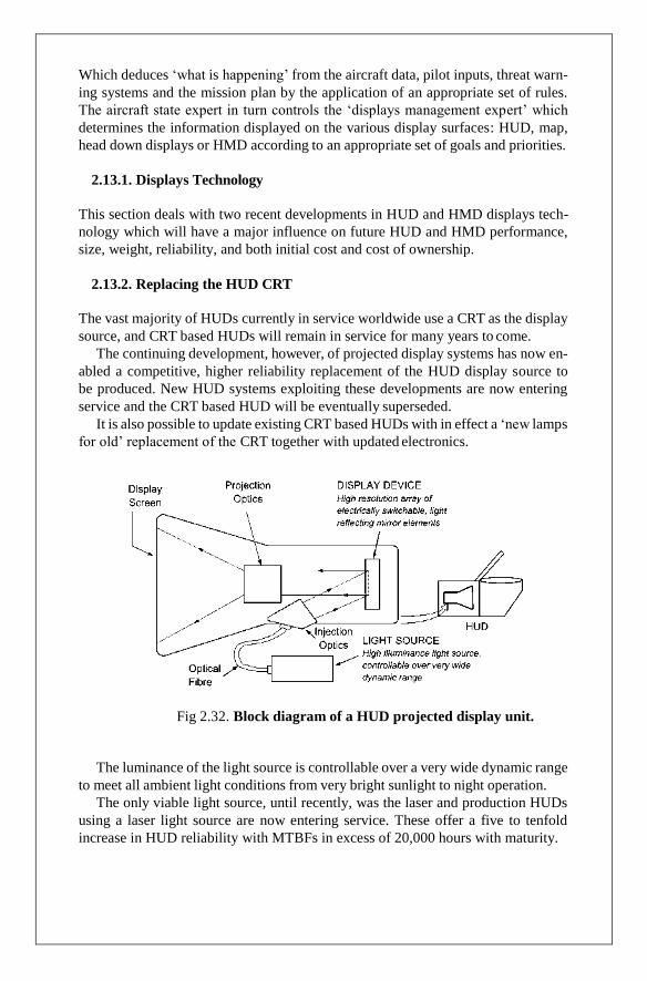
Which deduces ‘what is happening’ from the aircraft data, pilot inputs, threat warn-

ing systems and the mission plan by the application of an appropriate set of rules.

The aircraft state expert in turn controls the ‘displays management expert’ which

determines the information displayed on the various display surfaces: HUD, map,

head down displays or HMD according to an appropriate set of goals and priorities.

2.13.1. Displays Technology

This section deals with two recent developments in HUD and HMD displays tech-

nology which will have a major influence on future HUD and HMD performance,

size, weight, reliability, and both initial cost and cost of ownership.

2.13.2. Replacing the HUD CRT

The vast majority of HUDs currently in service worldwide use a CRT as the display

source, and CRT based HUDs will remain in service for many years to come.

The continuing development, however, of projected display systems has now en-

abled a competitive, higher reliability replacement of the HUD display source to

be produced. New HUD systems exploiting these developments are now entering

service and the CRT based HUD will be eventually superseded.

It is also possible to update existing CRT based HUDs with in effect a ‘new lamps

for old’ replacement of the CRT together with updated electronics.

Fig 2.32. Block diagram of a HUD projected display unit.

The luminance of the light source is controllable over a very wide dynamic range

to meet all ambient light conditions from very bright sunlight to night operation.

The only viable light source, until recently, was the laser and production HUDs

using a laser light source are now entering service. These offer a five to tenfold

increase in HUD reliability with MTBFs in excess of 20,000 hours with maturity.

Fig 2.33 ‘Digital Light Engine’ projector display unit (by courtesy of BAE

Systems).

Demonstrated very high reliability in a wide variety of civil and military display

applications. They are also widely used in very large screen projection systems to

display high definition video.

The Texas Instruments DMDTM is basically an array of over a million hinged

micro-mirrors which can be individually deflected mechanically through (12◦). Light modulation in a dark field projection system is achieved by tilting the micro-

Mirror to reflect light from the illuminating source on to, or away from the dis-

play screen. The micro-mirrors are matrix addressed and deflected by the electro-

static forces created by applying a voltage to the appropriate mirror electrodes; each

micro-mirror produces a display pixel.

2.13.3. HMD/HUD Optical System Technology

The preceding sections have covered the basic principles, functions and design of

HUDs and HMDs which are currently in service, and which will remain in service

for many years to come.

Fig 2.34. Block diagram of active CGH method of generating a fault tolerant

display.

Recent developments in holographic waveguide technology, however, will have

a profound impact on future HMD and HUD design. Exploitation of this technology

offers a major improvement in terms of mass, cost, volume, simplicity and optical

performance.

UNIT - III

COMMUNICATION AND NAVIGATION AIDS

3.1. Introduction

Gyroscopes (hereafter abbreviated to gyros) and accelerometers are known as in-

ertial sensors. This is because they exploit the property of inertia, namely the res-

istance to a change in momentum, to sense angular motion in the case of the gyro

and changes in linear motion in the case of the accelerometer.

They are fundamental to the control and guidance of an aircraft. For example, in a

FBW aircraft the rate gyros and accelerometers provide the aircraft motion feedback

which enables a man- oeuvre command control to be achieved and an

aerodynamically unstable aircraft to be stabilised by the flight control system (as

explained in Chapter 4).

Gyros and accelerometers are also the essential elements of the spatial reference

system or attitude/heading reference system (AHRS) and the inertial navigation sys-

tem (INS). They largely determine the performance and accuracy of these systems

and account for a major part of the system cost.

The AHRS and INS share common technology and operating principles. This

chapter covers gyros and accelerometers and attitude derivation from strap-down

gyros and accelerometers. It provides the basic background to inertial navigation

and AHRS systems, which are covered in Chapter 6 ‘Navigation Systems’.

3.2. Gyros and Accelerometers

The accuracy requirements for gyros and accelerometers can differ by several orders

of magnitude depending on the application.

Not surprisingly, the costs can also differ by an order of magnitude or more.

The quest for and attainment of the accuracies required for inertial navigation

have involved many billions of dollars expenditure worldwide and the continual ex-

ploitation of state of the art technology. For example, the world’s first laser was

demonstrated in 1960 and the first experimental ring laser gyro (RLG) was demon-

strated in 1963 with an accuracy of a few degrees per hour.

The first production RLG based inertial navigation systems (which requires

0.01◦/hour accuracy) went into large scale civil airline service in 1981. Strap-down RLG based IN systems now

dominate the market; a technology revolution

Fig 3.1. Tuning fork rate gyro.

ment suffers from the unacceptable characteristic that the smallest linear motions

applied to its base cause unacceptably large errors. To overcome the effect of base

motion, it is necessary to use balanced oscillations in which the oscillations of one

mass are counter-balanced by equal and opposite motion of a second equal mass.

Fig 3.2 Quartz rate sensor (courtesy of Systron Donner Inertial Division).

= ˙

Fig 3.3. Quartz rate sensor fabrication wafer with device overlaid (courtesy of

Systron Donner Inertial Division).

3.3. Optical Gyroscopes

3.3.1. Introduction

Optical gyroscopes such as the ring laser gyro and the fibre optic gyro measure

angular rate of rotation by sensing the resulting difference in the transit times for

laser light waves travelling around a closed path in opposite directions.

This time difference is proportional to the input rotation rate and the effect is

known as the ‘Sagnac effect’ after the French physicist G

The Sagnac effect time difference, OT , between the clockwise (cw) and anti-

clockwise (acw) paths is given by

OT 4A

θ

c2

where A is the area enclosed by the closed path, c the velocity of light and θ˙ the

angular rate of rotation about an axis normal to the plane of the closed path.

c

+ −

Fig 3.4. Sagnac interferometer. The clockwise and anti-clockwise waves interfere to produce a finge pattern which shifts when the interferometer is subjected to input rate, θ˙.

Fig 3.5. Sagnac effect.

OL = cOT

OL = 4A

θ

A rigorous derivation of the above formulae requires the use of the general theory

of relativity. A simpler kinematic explanation, however, is given below for the case

of a circular path in vacuo.

In time T , P has moved to P1 and the path length for the cw photon is equal to

(2πR RθT ) and the path length for the acw photon is equal to (2πR RθT ).

The difference in transit time,

Fig 3.6. Laser gyro schematic.

The IFOG operates basically as a Sagnac interferometer and measures the phase

shift in the fringe pattern produced by the input rotation rate. The accurate meas-

urement of very small Sagnac phase shifts has required the development of special

techniques which will be explained. The IFOG was initially developed to an AHRS

level of accuracy and the first large production orders for IFOG based AHRS were

placed in 1991. Development to inertial accuracy has since taken place in many

organisations and IFOG based IN systems are now available.

The resonator type of fibre optic gyro, or RFOG, operates in a similar manner to

the RLG but with the resonant ring of optical fibre driven by an external laser diode.

Two acousto-optical modulators are used to shift the laser frequency injected into the

cw and acw paths respectively with the modulation frequencies being controlled by

servo loops to maintain the resonance peak condition. The difference in the resonant

frequencies of the two paths is then directly proportional to the input rotation rate

as with the RLG. Development of the RFOG appears to be on the ‘back-burner’ at

the present time, as the IFOG type is giving an excellent all round performance.

Attention has thus been concentrated on the RLG and the IFOG.

3.4. The Interferometric Fibre Optic Gyro

The implementation of the interferometric type of FOG is best explained in a series

of stages starting with the simple basic system.

Light from the laser diode source is passed through a first beam splitter and a

single optical mode is selected. The light passes through a second beam splitter and

propagates in both directions around the fibre coil. In the absence of rotation, as

already explained, the transit times are identical so that when the light arrives back

at the second beam splitter, perfect constructive interference occurs with accompa-

nying fringe pattern. The gyro output signal is obtained by directing the returning

light via the first beam splitter to a photo-detector.

=

= ˙

= ˙

As explained, an input rotation rate about an axis normal to the plane of the coil

results in a difference in the transit times between the clockwise and anti-clockwise

beams as given by equation, viz.

OT 4A

θ

c2

If the fibre coil has N turns, A πR2 N where R is the mean radius of the coil, and

N can be expressed in terms of the length of the coil, L and the mean radius R, i.e.

Fig 3.7. Basic fibre optic gyro.

hence

L N =

2πR

OT LD

θ

c2

= = =

This transit time difference results in the Sagnac phase shift, given by

8s = ωOT

This phase shift between the clockwise and anti-clockwise travelling light waves

results in a reduction in the intensity of the light at the detector. This change in

intensity is very small for useful rotation rates and has required the development of

special techniques.

For example, a typical FOG with an optical path length L 200 m, coil diameter, D 70 mm and source laser wavelength 1.3 microns, when subjected to an input

rate of 10◦/sec will have a Sagnac phase shift of

2π × 200 × 70 × 10−2 ◦

8s = 1.3 × 10−6 × 3 × 10−8 × 10 = 2.26

Resolution of Earth’s rate (15◦/hour) requires the measurement of a phase shift

of 3.38 arc seconds. Resolution of 0.01◦/hour seems barely credible at first sight but is achievable as will be shown.

Fig 3.8. Phase modulation – open-loop IFOG.

The light intensity output signal from the photo-detector is converted to a digital

value by an A to D converter followed by digital demodulation and integration. The

loop is closed by driving the integrated optics phase modulator with a voltage ramp

whose slope is proportional to the input rate. This ramp produces a non-reciprocal

phase shift between the light waves so as to restore and maintain the sensor at the

zero rotation condition.

The advantages of the closed-loop system are:

(a) Output is independent of light source intensity variations as the system is al-

ways operated at null.

(b) Output is independent of the gains of individual components in the measure-

ment system as long as a very high open-loop gain is maintained.

(c) Output linearity and stability depend only on the phase transducer.

The voltage ramp driving the phase modulator generates a frequency difference

to null the phase difference produced by the input rate.

Fig 3.9Closed-loop interferometric FOG.

Frequency difference and phase shift are directly related. The phase shift, 8, that

light experiences in propagating along a single mode optical fibre of length, L, and

refractive index, n, is given by

= = =

nλ πD/4 λ(nπ D)

Fig 3.10. Fibre optic gyro inertial measuring unit (courtesy of Smiths

Industries).

i.e.

where K1 = D/nλ.

Of = K1θ

The output characteristic is thus the same as the RLG and the IFOG behaves as

an integrating rate gyro.

The scale factor stability is dependent on the stability of D, n and λ.

For the example FOG already used D 70 mm, λ 1.3 mm, n 1.5. Sub-

stituting these values, one output pulse corresponds to an angular increment of 5.75

arc seconds.

Equation (5.11) can be shown to be the same as the RLG output equation by

multiplying the numerator and denominator of (5.11) by πD/4, viz.

D

Of = πD/4

θ = 4A

θ

The equivalent optical perimeter (nπ D) corresponds to the RLG path length, L. The

inherent simplicity of the FOG and the use of Integrated Optic Chips where the

various electro-optical elements are integrated on to a substrate leads to low

manufacturing costs and the IFOG is a highly competitive gyro in terms of cost,

reliability, ruggedness and performance.

Integrated three axis versions are being produced with the three FOGs sharing the

same laser diode source.

= ×

m

+ +

+ + T L D

3.5. Accelerometers

3.5.1. Introduction – Specific Force Measurement

The acceleration of a vehicle can be determined by measuring the force required to

constrain a suspended mass so that it has the same acceleration as the vehicle on

which it is suspended, using Newton’s law: force mass acceleration.

The measurement is complicated by the fundamental fact that it is impossible

to distinguish between the force acting on the suspended mass due to the Earth’s

gravitational attraction and the force required to overcome the inertia and accelerate

the mass so that it has the same acceleration as the vehicle. The vehicle acceleration,

a, being produced by the vector sum of the external forces acting on the vehicle,

namely, the propulsive thrust, T, lift, L, drag, D, and the gravitational force, mg,

acting on the aircraft mass, m.

(The bold print denote the quantities are vector quantities.)

Fig 3.11. Simple spring restrained pendulous accelerometer.

T + L + D + mg = ma ( )

a = + g

The vector sum of the external forces excluding the gravitational force divided

by the aircraft mass, that is (T L D)/m, is known as the ‘specific force’. The

force, Fa, required to constrain the suspended mass, ma, is thus given by

Fa + mag = maa

Fa + g = a =

(T + L + D) + g

Hence

ma

Fa = ma

m

the accelerometer will thus measure the specific force component along its input

axis and not the vehicle acceleration component.

3.5.2. Simple Spring Restrained Pendulous Accelerometer

A simple spring restrained pendulous accelerometer is shown schematically. This

comprises an unbalanced pendulous mass which is restrained by the spring hinge

so that it can only move in one direction, that is along the input axis. The spring

hinge exerts a restoring torque which is proportional to the angular de- flection

from the null position. When the case is accelerated the pendulum deflects from

the null position until the spring torque is equal to the moment required to ac-

celerate the centre of mass of the pendulum at the same acceleration as the vehicle.

The transfer function of the simple accelerometer described is a simple quadratic

lag filter of the type

Output K0

Input Accln. =

D2 + 2ζ ω0D + ω02

K0 is the accelerometer scale factor, and the undamped natural frequency ω0

Fig 3.12. Torque balance pendulous accelerometer schematic.

(Strictly speaking, the specific force is measured.) Pulse torque operation of the

capture amplifier is generally used giving a pulse rate output which is directly

proportional to the input acceleration. Each pulse represents a velocity increment,

for example 0.05 m/s (0.1 knots approx.), providing an inherent integration.

Fig 3.13. ‘Solid state’ dry accelerometer construction.

Accelerometers used in very severe environments with very high vibration and

shock levels are generally oil filled to increase their robustness.

‘Solid state’ accelerometers fabricated from silicon using semi-conductor man-

ufacturing technology are now being widely used for lower accuracy applications.

The technology offers very small size and low manufacturing costs.

Fig 3.14. Torque balance accelerometer loop.

K

K

[ · + ]

given by

a = amax sin ωt

where amax is the peak value of the vibration acceleration, a, and ω is the angular

frequency.

The displacement of the pendulum from null is given by

ε = amax

sin(ωt + 8)

where K is dependent on the loop gain at frequency ω and 8 is the phase shift

between ε and a.

Sensed cross-axis acceleration is ε · amax sin ωt

a2

= max

sin ωt · sin(ωt + φ)

The product term sin ωt sin(ωt φ) has an average value of cos 8/2 so that

a proportion of the input vibration is rectified. This error source contributes to the

‘g2 error sensitivity’ of the accelerometer as it is proportional to the square of the

vibration acceleration.

Fig 3.14. Skewed axes sensors – dodecahedron configuration.

3.6. Skewed Axes Sensor Configurations

One of the attractive features of a strap-down system is that economical failure ab-

sorption configurations are available. One such configuration is an arrangement of

six single axis rate gyros and six accelerometers, with their input axes skewed with

respect to the principal axes

=

The gyro outputs denoted by letters A to F are functions of the body rates.

A = p sin α + r cos α B = −p sin α + r cos α C = p cos α + q sin α

D = p cos α − q sin α E = q cos α + r sin α F = q cos α − r sin α

where α 31.716747◦, the angle between the gyro input axes and the body axes.

There are thus six equations in three unknowns which can give two independent

measures of each body rate. Sophisticated algorithms can be used to isolate a failed

gyro and re-combine the data from the remaining sensors in an optimum way.

There are other configurations of skewed sensors which are also used. For ex- ample, three orthogonal sensors with their input axes aligned with the aircraft prin-

cipal axes and a fourth sensor with its input axis skewed at 45◦ to the principal

axes.

Two such independent sensor sub-assemblies can tolerate three gyro failures.

3.7. GPS – Global Positioning System

3.7.1. Introduction

GPS is basically a radio navigation system which derives the user’s position from

the radio signals transmitted from a number of orbiting satellites.

The fundamental difference between GPS and earlier radio navigation systems,

such as LORAN-C (now no longer in use), is simply the geometry of propagation

from ground based transmitters compared with space borne transmitters. An orbit-

ing satellite transmitter can provide line of sight propagation over vast areas of the

world. This avoids the inevitable trade-offs of less accuracy for greater range which

are inherent with systems using ground based transmitters. The satellite signals also

penetrate the ionosphere rather than being reflected by it so that the difficulties en-

countered with sky waves are avoided.

GPS provides a superior navigation capability to all previous radio navigation

systems. For these reasons and also space constraints, coverage of radio navigation

systems has been confined to GPS.

Satellite navigation can be said to have started with the successful launching by

the Russians of the world’s first orbiting satellite, SPUTNIK 1 in October 1957.

The development of the first satellite navigation system TRANSIT 1, was triggered

by observations made on the radio signals transmitted from SPUTNIK 1 and was

initiated at the end of 1958. TRANSIT 1 resulted in a worldwide navigation

system which has been in continuous operation since 1964.

Fig 3.15. Complementary filtered gyro/magnetic heading response to constant rate

of turn.

Fig 3.16. The GPS system.

A very similar satellite navigation system called GLONASS has been developed

by the Russians. Although designed for military applications (like GPS), it is avail-

able but is not being used elsewhere at the present time (2010).

3.8. GPS System Description

The overall GPS system comprises three segments, namely the space segment, the

control segment and the user segment and is shown schematically

Space Segment. This comprises 24 GPS satellites placed in six orbital planes at

55◦ to the equator in geo-synchronous orbits at 20,000 km above the Earth. The orbit tracks over the Earth, forming an ‘egg beater’ type pattern.

Twenty-one satellites are required for full worldwide coverage and three satellites

act as orbiting spares.

3.8.1. Basic Principles of GPS

The basic principle of position determination using the GPS system is to measure

the spherical ranges of the user from a minimum of four GPS satellites. The or-

bital positions of these satellites relative to the Earth are known to extremely high

accuracy and each satellite transmits its orbital position data.

Each satellite transmits a signal which is modulated with the C/A pseudo-random

code in a manner which allows the time of transmission to be recovered.

Fig 3.17. GPS spherical ranging.

The spherical range of the user from the individual transmitting satellite can be

determined by measuring the time delay for the satellite transmission to reach the

user.

Multiplying the time delay by the velocity of light then gives the spherical

range, R, of the user from the transmitting satellite. The user’s position hence lies

on the surface of a sphere of radius, R.

Fig 3.18. User–satellite geometry.

Fig 3.19. GPS satellite waveforms with perfect satellite clocks.

R1p = cOt1

R2p = cOt2

R3p = cOt3

R4p = cOt4

Let the range equivalent of the user’s clock offset be T , i.e.

T = cOT

Hence, from basic 3D co-ordinate geometry

R1 = [(X − X1)2 + (Y − Y1)

2 + (Z − Z1)

2]1/2 = R1p − T

R2 = [(X − X2)2 + (Y − Y2)

2 + (Z − Z2)

2]1/2 = R2p − T

R3 = [(X − X3)2 + (Y − Y3)

2 + (Z − Z3)

2]1/2 = R3p − T

R4 = [(X − X4)2 + (Y − Y4)

2 + (Z − Z4)

2]1/2 = R4p – T

when R1, R2, R3, R4 are the actual ranges from the user’s position to the four satel-

lites S1, S2, S3, S4 and the coordinates of these satellites are (X1 Y1 Z1), (X2 Y2

Z2), (X3 Y3 Z3), (X4 Y4 Z4) respectively.

.

Each satellite time is related to GPS time by a mathematical expression and the

user corrects the satellite time to the GPS time using the equation

t = ts/c − Ots/c

where t is the GPS time in seconds, ts/c is the effective satellite time at signal trans-

mission in seconds and Ots/c is the time offset between the satellite and GPS master

time.

The time offset is Ots/c computed from the following equation

Ots/c = a0 + a1(t − to/c) + a2(t − to/c)2 + Otr

where a0, a1, and a2 are polynomial coefficients representing the phase offset, fre-

quency offset and ageing term of the satellite clock with respect to the GPS master

time and Otr is the relativistic term (seconds). The parameter t is the GPS time and

to/c is the epoch time at which the polynomial coefficients are referenced and gener-

ally to/c is chosen at the mid point of the fit interval. The polynomial coefficients a0,

a1, a2 are estimated by the control segment for each satellite clock and periodically

uplinked to the satellite.

These coefficients are transmitted together with the satellite orbital position data,

termed the Ephemeris parameters, to the navigation user equipment as navigation

messages. The clock corrections for the four satellites are designated τ1, τ2, τ3, and

τ4.

The spherical ranges R1, R2, R3 and R4 are thus given by

R1 = c(Ot1 + OT − τ1) R2

= c(Ot2 + OT − τ2) R3 =

c(Ot3 + OT − τ3)

R4 = c(Ot4 + OT − τ4)

All satellite clocks are mathematically synchronised to the GPS master time by

means of these clock correction terms. The error in synchronisation will grow, how-

ever, if the polynomial coefficients a0, a1 and a2 are not updated periodically.

Fig 3.20. Satellite-Earth geometry. Ephemeris parameter definition.

The navigation equations are basically non-linear as can be seen in equa-

tions (6.56), (6.57), (6.58) and (6.59), but can be linearised about nominal values

for their solution by applying Taylor’s series approximations.

3.8.2. Integration of GPS and INS

GPS and INS are wholly complementary and their information can be combined to

the mutual benefit of both systems. For example:

Calibration and correction of INS errors – the GPS enables very accurate cal-

ibration and correction of the INS errors in flight by means of a Kalman filter.

The INS can smooth out the step change in the GPS position output which can

occur when switching to another satellite because of the change in inherent

errors.

Jamming resistance – like any radio system, GPS can be jammed, albeit over a

local area, although it can be given a high degree of resistance to jamming. The

INS, having had its errors previously corrected by the Kalman filter, is able to

provide accurate navigation information when the aircraft is flying over areas

subjected to severe jamming.

Antenna obscuration – GPS is a line of sight system and it is possible for the

GPS antenna to be obstructed by the terrain or aircraft structure during man-

oeuvres.

Antenna location corrections – the GPS derived position is valid at the antenna

and needs to be corrected for reference to the INS location. The INS provides

attitude information which together with the lever arm constants enables this

correction to be made.

•

•

•

•

•

3.9. Differential GPS

3.9.1. Introduction

As explained in the preceding section the horizontal position accuracy available to

all GPS users (civil and military) is now 16 m. This was not the case, however, until

2000 when the restriction of ‘Selective Availability’ was removed.

Concerns about potential enemies using GPS to deliver missiles and other

weapons against the US had led to a policy of accuracy denial, generally known

as Selective Availability. The GPS ground stations deliberately introduced satellite

timing errors to reduce the positioning accuracy available to civil users to a hori-

zontal positioning accuracy of 100 m to a 95% probability level.

Fig 3.21. The differential GPS concept.

DGPS can be defined as:

The positioning of a mobile station in real-time by corrected (and possibly

Doppler or phase smoothed) GPS pseudo ranges.

The corrections are determ- ined at a static ‘reference station’ and transmitted

to the mobile station. A monitor station may be part of the system, as a quality

check on the reference station transmissions.

The success of DGPS can be seen from its application to new markets such as loc-

ating land vehicles used by the emergency services. Successful trials for automatic

landings and taxi-way guidance have also been conducted.

It is now widely used in land and hydrographic surveying applications.

3.9.2. Basic Principles

The basic principle underlying DGPS is the fact that the errors experienced by two

receivers simultaneously tracking a satellite at two locations fairly close to each

other will largely be common to both receivers.

The basic differential GPS concept is illustrated. The position of the stationary

GPS Reference Station is known to very high accuracy so that the satellite ranges

can be very accurately determined, knowing the satellite ephemeris data.

Fig 3.22. GPS error sources.

The errors in the pseudo-range measurements can then be derived and the required

corrections computed and transmitted to the user’s receiver over a radio link. The

errors present in a GPS system are illustrated

GPS satellite clocks. GPS satellites are equipped with very accurate atomic

clocks and corrections are made via the Ground Stations, as explained in the pre-

ceding section.

Summary of GPS error sources.

Typical error budget (in metres)

Per satellite accuracy Standard GPS Differential

GPS

Satellite clocks 1.5 0 Orbit errors 2.5 0 Ionosphere 5.0 0.4 Troposphere 0.5 0.2 Selective availability∗ 30.0 0 Receiver noise 0.3 0.3 Multi-path (reflections) 0.6 0.6

Typical positioning

accuracy

Horizontal 50.0 1.3 Vertical 78.0 2.0 3D 93.0 2.8

∗Note: Selective Availability error is shown to demonstrate the effectiveness of the

DGPS technique, although the Selective Availability restriction has now been

removed.

A predicted correction factor for the Earth’s atmosphere path is made in the re-

ceiver but this is based on a statistical model and there are inevitable residual errors

present.

Multi-path errors. The GPS satellite signal is received by the direct line of sight

(LOS) path, but the signal may also be received as the result of reflections off local

obstructions.

Fig 3.23. Simplified functional diagram of a generic differential GPS system.

The satellite pseudo-range measurement in the user’s GPS receiver is carried out

by the correlation of the received satellite signal with the receiver generated replica

of the known satellite C/A code using a code tracking loop. The accuracy of the

time measurement by the C/A code tracking loop is inevitably ultimately limited by

noise sources such as multi-path reception.

Fig 3.24. Remote air traffic control.

GPS receivers also employ carrier tracking loops to monitor the Doppler shifted

carrier component of the satellite navigation signals. The Doppler shift is propor-

tional to the radial velocity of the receiver relative to the satellite. The velocity of

the user vehicle is computed from these Doppler shifts.

The Ground Reference GPS Station in the DGPS system uses these Doppler

frequency shift measurements to improve the accuracy of the pseudo-range meas-

urements. Integrating the Doppler shift over an interval provides a measurement of

the change in satellite-to-receiver range.

Future Augmented Satellite Navigation Systems

The advent of satellite navigation systems and satellite communication links has

provided new capabilities for aircraft precision navigation, particularly in civil op-

erations.

Providing the integrity and accuracy requirements can be met, satellite naviga-

tion systems are able to support all phases of flight including all-weather precision

approaches to airports not equipped with ILS (or MLS) installations.

Successful concept proving trials were, in fact, conducted by the UK Air Traffic

Control authorities in conjunction with British Airways around 1996. The trials used

the on-board GPS receivers and SAT COM radios in a British Airways Boeing 747

airliner to monitor the aircraft flight paths on normal commercial flights to the West

Indies.

Fig 3.25. Wide area augmentation system, WAAS, concept.

Extensive trials of a WAAS evaluation system have been conducted by the FAA

over the last decade, with very promising results. It appears very likely that the full

system will be built and become operational over the next decade.

UNIT - IV

MILITARY AIRCRAFT ADAPTATION

4.1. Introduction and Basic Principles

The dictionary definition of navigation is a good one.

Navigation – The act, science or art of directing the movement of a ship or

aircraft.

Navigation thus involves both control of the aircraft’s flight path and the guidance

for its mission.

The measurement of the aircraft’s attitude with respect to the horizontal plane in

terms of the pitch and bank angles and its heading, that is the direction in which it

is pointing in the horizontal plane with respect to North, is essential for both control

and guidance.

This information is vital for the pilot in order to fly the aircraft safely in all

weather conditions, including those when the normal visibility of the horizon and

landmarks is poor or not available, for example in haze or fog conditions, flying in

cloud and night flying. Attitude and heading information is also essential for the

key avionic systems which enable the crew to carry out the aircraft’s mission. These

systems include the autopilot system (e.g., Attitude and Heading Hold modes, Auto-

land, etc.) navigation system and the weapon aiming system. The information is also

required for pointing radar beams and infrared sensors.

.

In order of increasing accuracy these are:

1. Air data based DR navigation. The basic information used comprises the true

airspeed (from the air data computer) with wind speed and direction (forecast

or estimated) and the aircraft heading from the Attitude Heading Reference

System, (AHRS).

2. Doppler/heading reference systems. These use a Doppler radar velocity sensor

system to measure the aircraft’s ground speed and drift angle. The aircraft

heading is provided by the AHRS.

3. Inertial navigation systems. These derive the aircraft’s velocity components by

integrating the horizontal components of the aircraft’s acceleration with respect

to time. These components are computed from the outputs of very high accur-

acy gyroscopes and accelerometers which measure the aircraft’s angular and

linear motion.

4. Doppler inertial navigation systems. These combine the Doppler and INS out-

puts, generally by means of a Kalman filter, to achieve increased DR navigation

accuracy.

The primary DR navigation system which is also the primary source of very accurate

attitude and heading information is the Inertial Navigation System (INS). The term

Inertial Reference System (IRS), is also used in civil aircraft. The IRS can have

a lower inertial navigation accuracy of up to 4 NM/hour error compared with 1

to 2 NM/hour for a typical INS.

The attitude and heading accuracy, however, is still very high. The terminology

INS/IRS is used in this chapter to show they are essentially the same.

The main position fixing navigation systems in current use are briefly summar-

ised below.

(1) Range and Bearing (‘R/θ’) Radio Navigation Aids

These comprise VOR/DME and TACAN.

VOR (VHF omni-directional range) is an internationally designated short-

distance radio navigation aid and is an integral part of Air Traffic Control proced-

ures.

(2) Satellite Navigation Systems – GPS (Global Position System)

GPS is the most important and accurate position fixing system developed to date. It

is being used by every type of vehicle – aircraft – ships – land vehicles. Civilian use

is now very widespread, for example, GPS receivers are fitted in very many cars,

vans and lorries and they are readily affordable for ramblers.

The equipment required by the GPS user is entirely passive and requires a GPS

receiver only. Electronic miniaturisation has enabled very compact and light weight

GPS receivers to be produced.

Fig 4.1. Navigation system information flow to user systems.

R

˙ =

R

0

¸

0

¸

Terrain reference navigation systems derive the vehicle’s position by correlating the

terrain measurements made by a sensor in the vehicle with the known terrain feature

data in the vicinity of the DR estimated position. The terrain feature data is obtained

from a stored digital map database.

4.2. Basic Navigation Definitions

A very brief review of the terms and quantities used in navigation is set out below.

Position on the Earth’s surface is generally specified in terms of latitude and lon-

gitude co-ordinates which provide a circular grid over the surface of the Earth. The

Earth is basically a sphere – the variation in the radius of the Earth is only about

40 NM in a radius of 3,438 NM at the equator, being slightly flattened at the poles

(this variation is taken into account in the navigation computations).

Basic DR Navigation Systems

The basic principles of deriving a DR navigation position estimate are explained

below. The following quantities are required:

1. Initial position – latitude/longitude.

2. The northerly and easterly velocity components of the aircraft, VN and VE.

Referring to figure it can be seen that the rate of change of latitude is

the rate of change of longitude is

i.e.

λ = VN

µ VE

R cos λ

µ = VE

sec λ

The change in latitude over time, t, is thus equal to 1/R t VN dt and hence the

present latitude at time t can be computed given the initial latitude λ0.

Similarly, the change in longitude is equal to 1/R t VE sec λdt and hence the

present longitude can be computed given the initial longitude, µ0, viz.

It can be seen that a mathematical singularity is approached as λ approaches 90◦

and sec λ approaches infinity. This method of computing the latitude and longitude

of the DR position is hence limited to latitudes below 80◦.

A different co-ordinate reference frame is used to deal with high latitudes as will be explained later.

Fig 4.2 Derivation of rates of change of latitude and longitude.

Fig 4.3. Doppler/heading reference DR navigation system.

Hence

VN = VG cos ψT VE

= VG sin ψT

In the case of an air data based DR navigation system the northerly and easterly

velocity components of the aircraft can be derived as follows:

1. The horizontal velocity component VH of the true airspeed VT is obtained by

resolving VT through the aircraft pitch angle θ , viz.

VH = VT cos θ

2. The northerly and easterly velocity components of the airspeed are then derived

by resolving VH through the aircraft heading angle ψ, viz.

Northerly airspeed = VH cos ψ

Easterly airspeed = VH sin ψ

3. The forecast (or estimated) wind speed VW and direction ψW is resolved into

its northerly and easterly components, viz.

Northerly wind component = VW cos ψW

Easterly wind component = VW sin ψW

4. The northerly and easterly velocity components of the aircraft are then given

by:

VN = VH cos ψ + VW cos ψW (6.5)

VE = VH sin ψ + VW sin ψW (6.6)

Such a system provides a reversionary DR navigation system in the absence of

Doppler (or an INS) and would generally be used in conjunction with a radio nav-

igation system.

4.3. Inertial Navigation

4.3.1. Introduction

It is instructive to briefly review the reasons for the development of inertial naviga-

tion and its importance as an aircraft state sensor.

The attributes of an ideal navigation and guidance system for military applica-

tions can be summarised as follows:

• High accuracy

• Self-contained

• Autonomous – does not depend on other systems

• Passive – does not radiate

• Unjammable

• Does not require reference to the ground or outside world.

In the late 1940s these attributes constituted a ‘wish list’ and indicated the develop-

ment of inertial navigation as the only system which could be capable of meeting

all these requirements. It was thus initially developed in the early 1950s for the nav-

igation and guidance of ballistic missiles, strategic bombers, ships and submarines

(Ships Inertial Navigation System, SINS).

Accurate position in whatever coordinates are required – e.g. latit-

ude/longitude, etc.

• Ground speed and track angle.

• Euler angles: heading, pitch and roll to very high accuracy.

Fig 4.4. Basic principles of inertial navigation.

• Aircraft velocity vector (in conjunction with the air data system).

Accurate velocity vector information together with an accurate vertical reference

are essential for accurate weapon aiming and this has led to the INS being installed

in military strike aircraft from the early 1960s onwards as a key element of the

navigation/weapon aiming system.

4.3.2. Initial Alignment and Gyro Compassing

Inertial navigation can only be as accurate as the initial conditions which are set

in. It is therefore essential to know the orientation of the accelerometer measuring

axes with respect to the gravitational vector, the direction of true North, the initial

position and the initial velocity components to very high accuracy.

The two basic references used to align an inertial system are the Earth’s gravita-

tional vector and the Earth’s rotation vector.

The initial alignment process is basically the same in a stable platform and strap-

down INS.

The difference being that in a stable platform INS, the stable platform is

physically rotated to bring it into alignment with the local NED axes by applying

precession torques to the vertical and azimuth gyros on the platform.

It is thus easier to visualise (literally). Whereas the strap-down system carries

out the axis rotations within the system computer to create, in effect, a virtual stable

platform as explained earlier.

The North pointing virtual accelerometer will hence be tilting away from the

horizontal at a rate K cos λ.Oψ in the absence of any levelling or gyro compassing

•

Fig 4.5. Fine levelling and gyro compassing loops.

loops. (This is assuming the appropriate corrections are made to compensate for

K cos λ and K sin λ respectively.)

The gyro compassing loop adjusts the computed heading until the east compon-

ent of the gyro angular rate measurement in the horizontal plane is nulled, the angu-

lar rate of rotation about the East axis being estimated from the summed East axis

OθE =

K cos λ.Oψdt)

The allowable gyro drift rate uncertainty can be determined from the accuracy re-

quired of the heading alignment. For example, if an accuracy of 0.1◦ is required for

a latitude of 45◦, then the component of the Earth’s rate sensed at this latitude with

a misalignment of 0.1◦ is equal to (0.1/57.3) sin 45◦ degrees per hour, that is 0.017

degrees per hour.

It can be seen that the magnitude of the component of Earth’s rate to be sensed decreases with increasing latitude, so that gyro compassing is effectively restricted

to latitudes below 80◦.

The major factors which affect alignment accuracy and alignment times are:

(a) Initial tilt.

(b) Aircraft movements, e.g., effect of wind gusts etc.

(c) Accelerometer bias errors and gyro drift rates.

(d) Change of the above quantities (c) with time as the system warms up.

(e) Accelerometer resolution and gyro threshold.

The loop gains in the levelling and gyro compassing loops are generally con-

trolled by means of a Kalman filter to give an optimal alignment process. Typical

alignment times are of the order of seven minutes for full accuracy IN performance.

=

E N

Reduced alignment times are sometimes used and the system corrected to give

full IN accuracy by subsequent position fixes using a position fixing navigation

system (e.g., GPS).

4.3.3. Effect of Azimuth Gyro Drift

The effect of azimuth gyro drift is to cause position errors which build up with time

and are a function of azimuth error, aircraft velocity and latitude.

From the previous section on gyro compassing it can be seen that an azimuth er- ror Oψ, will effectively inject a drift of K cos λ.Oψ about the East axis. An error of

0.2◦ for instance, would generate an effective drift of 0.033◦/hour (two minutes of

arc/hour approximately).

4.3.4. Vertical Navigation Channel

It has been shown in Section 6.2.2 that Schuler tuning effectively constrains the error

build up with time in the horizontal channels of the INS. Unfortunately, however,

there is no such action in the vertical channel and small errors in computing the

vertical acceleration correction terms are integrated with time – in fact the vertical

distance error builds up exponentially with time. As explained earlier, the principal

correction terms for the vertical accelerometer channel are:

(i) Gravity – gravity varies with altitude according to the inverse square law. The

gravitational acceleration at an altitude H is given by

R2

g = g0 0

(R0 + H)2

where g0 = gravitational acceleration at the earth’s surface.

Errors in correcting for the variation in gravitational acceleration with height

result in a vertical distance error which builds up as cosh function of time. Also,

gravity varies over the Earth’s surface and has anomalous values in certain

places.

(ii) Centrifugal acceleration – a vehicle moving over the Earth’s surface is describ- ing a circular trajectory in space and so will experience a centrifugal acceler- ation (V

2 + V

2 )/R where VE and VN are the easterly and northerly velocity

components of the vehicle respectively. (iii) Coriolis acceleration – the component of the Earth’s rotation rate K cos λ about

the North axis is combined with the easterly velocity VE and generates a Cori-

Consider first the simple second-order mixing system shown in bold. The

baro-inertial feedback loop is capable of being opened and the gains K1 and

K2 which determine the damping and response times respectively are also

capable of being varied. The system response can be shown to be given by

+ + + + + +

D2 (K2 + K1D) 1

HI = (D2 K1D K2)

·H + (D2 K1D K2)

·HP + (D2 K1D K2)

·OaD

(6.21)

where H is the true height, HP is the pressure altitude, OaD is the uncorrected

vertical acceleration error and HI is the baro/inertial mixed height.

The inertially derived component of HI , that is

D2

(D2 + K1D + K2) · H

(a)

(b)

Fig 4.6 (a) Baro-inertial mixing. Simple second-order baro-inertial mixing shown

in bold lines. Integral term correction for inertial drift shown in dotted lines. (b)

Fourth-order baro-inertial mix- ing (with correction for inertial channel drift and

pressure altitude error).

couples the inertially measured height through a second-order high pass filter trans-

fer function which responds to dynamic changes in height without lag, but ‘DC

blocks’ the steady-state value.

The barometrically derived component of HI , that is

(K2 + K1D)

(D2 + K1D + K2) · HP

couples the barometrically derived height through a low pass filter which smooths

the pressure height signal and attenuates the noise present in the signal. The dy-

namic response is thus slugged by the low pass filter but the steady-state value of

the pressure height is not affected. The combination of the two components results

in a fast response with a low noise content.

4.3.5. Choice of Navigation Co-ordinates

The choice of a navigation co-ordinate system reduces practically to either:

(a) Spherical co-ordinates (latitude/longitude).

(b) Direction cosines.

A spherical co-ordinate system has two mathematical ‘poles’ or singularities where

the value of one co-ordinate (the longitude) is indeterminate and near which the

high rates of change of that co-ordinate make any system implementation imprac-

tical (longitude rate µ = (VE/R) sec λ becomes infinite when λ = 90◦).

With the latitude/longitude co-ordinate system (also known as the geographical or

‘geodetic’ system) these poles are the true North and South poles of the Earth.

This co-ordinate system is satisfactory provided there is no requirement for navigation

in the polar regions. It also provides the latitude/longitude information for display to

the flight crew.

When polar navigational capability is required there are three possible ways to

overcome the difficultly, namely:

(a) A spherical co-ordinate system with the poles removed to some other regions.

(b) A ‘unipolar’ system.

(c) Direction cosines.

The spherical co-ordinate system with transferred poles gives rise to added complic-

ations in the ellipsoidal corrections because of the asymmetry which results from the

misalignment between the main co-ordinate axis and the axis of the geographic el-

lipsoid. More seriously, it is a solution of limited usefulness because the singularities

still exist.

.

Fig 4.7. Strap-down INS computing flow diagram.

4.3.6. Strap-down IN System Computing

The basic computing flow diagram for a strap-down INS is shown in. A strap-down

IN system carries out the same functions as a stable platform type. INS and many

elements and functional areas are common to both systems. There are two crucial

areas in the strap-down mechanisation. These are:

1. Attitude integration whereby the vehicle attitude is derived by an integration

process from the body incremental angular rotations measured by the gyros.

2. Accelerometer resolution whereby the corrected outputs of the body mounted

accelerometers are suitably resolved to produce the horizontal and vertical ac-

celeration components of the aircraft.

The derivation of the aircraft attitude from the strap-down gyro outputs by con-

tinuously updating the four

Fig 4.8. Solid state modular implementation of a strap-down INS.

The derivation of the equivalent (or virtual) horizontal and vertical accelerometer

outputs from the body mounted accelerometers is as explained in Chapter 5, Sec-

tion 5.3.2.2, using the Direction Cosine Matrix derived from the Euler parameters.

The computing system, after deriving the equivalent North, East, Down acceler-

ometer outputs and transforming the co-ordinate frame rates from local NED axes

to aircraft body axes, is then the same as for a stable platform mechanisation.

The implementation of a strap-down INS is shown. The aim is to give the

reader an appreciation of the small number of solid state modules required. These

comprise:

1. The Inertial Measuring Unit (IMU) comprising three orthogonally mounted

laser gyros and three orthogonally mounted accelerometers.

2. The Processor Module carrying out all the processing tasks just described, and

also monitoring and self test functions.

3. The Interface Module carrying out all the interfacing tasks.

4. The Power Supply Unit.

The complexity resides in the software and the processor and interface micro-chips.

The Honeywell Laseref VI Micro Inertial Reference System is an example of a

current state of the art INS. The inset illustration and data are published by courtesy

of Honeywell.

564

• Overall size: 6.5jj × 6.4jj × 6.4jj 16.5 cm × 12.3 cm × 12.3 cm)

• Weight: 9.1 lbs (4.14 kg)

• Power consumption: 20 watts

• Reliability > 50,000 hours

Position accuracy (unaided) is 2 NM/hour.

The inertial sensors comprise the Honeywell GG 1320 AN Digital Laser Gyro and

the QA 2000 Q Flex Accelerometer, a closed-loop, torque balance accelerometer.

The system incorporates GPS integration. Hybrid mode position and velocity ac-

curacy is 12 metres and 0.25 knots (0.13 m/s). GPS integration also enables IRS

alignment in motion and even despatch prior to navigation mode. This feature elim-

inates delays while waiting for the IRS to align.

4.4. Aided IN Systems and Kalman Filters

The time dependent error growth of an IN system makes it necessary that some form

of aided navigation system using an alternative navigation source is introduced to

correct the INS error build up on long distance flights. For example, as mentioned

earlier, a good quality unaided INS of 1 NM/hour accuracy could have a positional

error of 5 NM after a five hour flight.

A variety of navigation aids can be used for this purpose, for example GPS.

Fig 4.9. Aided INS with simple positional reset.

To recap, the various navigation sources comprise:

1. Position Data

• GPS, VOR/DME, TACAN.

• Terrain reference navigation systems.

565

• Radar.

• Visual fixes (e.g., use of helmet mounted sight).

• Astro (Stellar) navigation (using automatic star trackers).

2. Velocity Data

• Doppler radar.

• GPS.

3. Altitude Data

• Barometric altitude from the air data computer.

• Radio altimeter.

These sources provide good information on the average at low frequency but are

subject to high frequency noise due to causes such as instrument noise, atmospheric

effects, antenna oscillation, unlevel ground effects, etc.

Fig 4.10. Block diagram of aided IN system with Kalman filter.

Fig 4.11. Aided INS with Kalman filter.

566

however, is poor due to the inherent long term drift characteristics, as already ex-

plained.

It should be stressed at this point that a Kalman filter can be used to provide an

optimum estimate of the errors in any measuring system and its use is not confined to

navigation systems, although it has been particularly effective in this field. Examples

of other applications include:

• Radar and infrared automatic tracking systems.

• Fault detection and in monitoring of multiple (redundant) sensors.

• Initial alignment and gyro compassing of an INS.

Fig 4.12. Application of Kalman filters to mixed navigation systems.

The Kalman filter was first introduced in 1960 by Dr. Richard Kalman (see reference

list at the end of this chapter). It is essentially an optimal, recursive data processing

algorithm which processes sensor measurements to estimate the quantities of in-

terest (states) of the system using:

1. A knowledge of the system and the measurement device dynamics.

2. A statistical model of the system model uncertainties, noises, measurement

errors.

3. Initial condition information.

UNIT - V

AIRBORNE RADAR, ASTRIONICS - AVIONICS FOR SPACECRAFT

5.1. Introduction

Autopilots and flight management systems (FMS) have been grouped together in

one chapter as modern aircraft require a very close degree of integration between

the two systems, particularly in their respective control laws.

Much of the background to the understanding of autopilots has been covered

in earlier chapters. For instance, the dynamics of aircraft control and fly-by-wire

flight control systems, including pitch rate and roll rate manoeuvre command

control systems. Chapter 4 also covers the meth- ods used to achieve the very high

integrity and safety required to implement FBW flight control through the use of

redundancy.

Similar levels of safety and integrity are required in some autopilot modes, for

example automatic landing and automatic terrain following (T/F). The digital

implementation of flight control systems is also covered.

The autopilot is thus an essential equipment for most military and civil aircraft,

including helicopters. The advent of the micro-processor has also enabled relatively

sophisticated and affordable autopilots to be installed in large numbers of general

aviation type aircraft.

The prime role of the flight management system is to assist the pilot in managing

the flight in an optimum manner by automating as many of the tasks as appropriate

to reduce the pilot workload. The FMS thus performs a number of functions, such

as:

• Automatic navigation and guidance including ‘4D’ navigation.

• Presentation of information.

• Management of aircraft systems.

• Efficient management of fuel.

• Reduction of operating costs.

The broad concepts and operation of an FMS are covered in Section 8.3. It should

be appreciated that the detailed implementation of an FMS is a complex subject and

can involve over 100 man-years of software engineering effort and very extensive

(and expensive) flight trials before certification of the system can be obtained from

the regulatory authorities. It is only possible, therefore, because of space constraints

to give an overview of the subject.

It should also be pointed out that an FMS has an equally important role in

a military aircraft. Accurate adherence to an optimum flight path and the abil-

ity to keep a rendezvous at a particular position and time for, say, flight re-

fuelling or to join up with other co-operating aircraft are clearly very important

requirements.

Fig 5.1 Autopilot loop.

5.2. Autopilots

5.2.1. Basic Principles

The basic loop through which the autopilot controls the aircraft’s flight path is shown

in the block diagram

The autopilot exercises a guidance function in the outer loop and generates

commands to the inner flight control loop.

These com- mands are generally attitude commands which operate the aircraft’s

control surfaces through a closed-loop control system so that the aircraft rotates

about the pitch and roll axes until the measured pitch and bank angles are equal to

the commanded angles.

The changes in the aircraft’s pitch and bank angles then cause the aircraft flight

path to change through the flight path kinematics.

For example, to correct a vertical deviation from the desired flight path, the air-

craft’s pitch attitude is controlled to increase or decrease the angular inclination of

the flight path vector to the horizontal. The resulting vertical velocity component

thus causes the aircraft to climb or dive so as to correct the vertical displacement

from the desired flight path.

To correct a lateral displacement from the desired flight path requires the aircraft

to bank in order to turn and produce a controlled change in the heading so as to

correct the error.

The pitch attitude control loop and the heading control loop, with its inner loop

commanding the aircraft bank angle, are thus fundamental inner loops in most auto-

pilot control modes.

The outer autopilot loop is thus essentially a slower, longer period control loop

compared with the inner flight control loops which are faster, shorter period loops.

= −

g

Fig 5. 2. Height control (heavy lines show FBW pitch rate command loop). Pitch

rate gyro and AHRS are shown separately for clarity. In a modern aircraft, a strap-

down AHRS/INS provides both θ and q outputs.

5.2.2. Height Control

Height is controlled by altering the pitch attitude of the aircraft, as just explained.

The basic height control autopilot loop is shown in figure.

The pitch rate command inner loop provided by the pitch rate gyro feedback en-

ables a fast and well damped response to be achieved by the pitch attitude command

autopilot loop. As mentioned earlier, a FBW pitch rate command flight control sys-

tem greatly assists the autopilot integration.

The pitch attitude loop bandwidth thus determines the bandwidth of the height

loop so that the importance of achieving a fast pitch attitude response can be seen.

The transfer function of the flight path kinematics is derived as follows. Vertical

component of the aircraft’s velocity vector is

VT sin θF = H˙

5.2.3. Heading Control Autopilot

The function of the heading control mode of the autopilot is to automatically steer

the aircraft along a particular set direction. As explained in Chapter 3, Section 3.5,

aircraft bank to turn, and assuming a perfectly co-ordinated turn (i.e. no sideslip).

Hence, for small bank angles

W = U

8

The basic control law used to control the aircraft heading is thus to demand a

bank angle, 8D, which is proportional to the heading error, WE (WCOM W),

where WCOM is the commanded heading angle and W the heading angle.

8D = KW · WE

where Kψ is the heading error gain.

Fig 5.3. Heading control loop (heavy lines show FBW roll rate command loop).

Roll rate gyro and AHRS are shown separately for clarity. In a modern aircraft, a

strap-down AHRS/INS provides both p and 8 outputs.

However, a good appreciation of the aircraft and autopilot behaviour can be ob-

tained by assuming pure rolling motion and neglecting the effects of cross-coupling

between the roll and yaw axes.

This can also be justified to some extent by assuming effective auto-stabilisation

loops which minimise the cross-coupling effects.

8 = p + q sin 8 tan θ + r cos 8 tan θ

These assumptions are used in the worked example which follows in order to sim-

plify the aircraft dynamics.

It is also assumed that there is no loss of height when the aircraft banks to correct

heading, appropriate changes to the pitch attitude and hence incidence being

effected by the height hold autopilot control.

= =

=

= −

E

D

Fig 5.4. Block diagram of bank angle demand loop.@

5.3. Worked Example of Heading Control Autopilot

The aircraft in this example has a roll rate response time constant TR 0.5 seconds

and Lp/Lξ 20◦/second per degree aileron deflection.

The response of the aileron servo actuators approximates to that of a simple first-

order filter with a time constant of 0.08 seconds. The aircraft’s forward velocity,

U 250 m/sec (approximately 500 knots) and is assumed to be constant.

Determine suitable values for the autopilot gains (or gearings) Kp, Kφ and Kψ .

The overall loop for the heading control is as shown in figure. The block diagram

for the bank angle demand loop is shown in figure.

It should be noted that the Laplace operator, s, has been substituted for operator

D(d/dt).

Determination of Roll Rate Eerror Gain, Kp

The open-loop transfer function of the innermost loop, namely, the roll rate feedback

loop is p Kp20

p =

(1 + 0.08s)(1 + 0.5s) = KG(s)

where pE pD p.

The closed-loop transfer function p/pD is given by

p KG(s)

p =

1 + KG(s)

The stability of the closed loop is determined by the roots of the characteristic equa-

tion

1 + KG(s) = 0

i.e.

0

. Σ

= × = =

0

Fig 5. 5. Roll rate response.

(1 + 0.08s)(1 + 0.5s) + 20Kp = 0

s2 + 14.5s + 25 1 + 20Kp = 0

Comparing with the standard form of second-order equation

2ζω0 = 14.5

ω2 = 25(1 + 20Kp)

Choosing a damping ratio, ζ 0.7, requires the undamped natural frequency,

ω0 10.4 rad/sec (14.5/2 0.7). From which Kp 0.165◦ aileron angle per degree/second roll rate error.

Kp = 0.165 seconds

p 0.767 p

= 2ζ 1

2

D 1 + ω0 s +

ω2 s

where ω0 = 10.4 and ζ = 0.7.

Σ

ω0

Σ

ω0

..

.

.ω

...

.

·

.

E s 1 + 2ζ

s + 1 s2

E .

ω0

Σ

ω0

Determination of Bank Angle Error Gain, Kφ

Consider now the bank angle demand loop. The open-loop transfer function is

8

8 = .

0.767Kφ

ω 2 0

where ω0 = 10.4 and ζ = 0.7.

The value of Kφ is determined using frequency response methods, as follows.

The open-loop frequency response can be obtained by substituting jω for s.

8

8 (jω) =

K

jω

.

1 − ω

2

+ j 2ζ ω

where K = 0.767Kφ.

= KF1 (jω) · F2 (jω)

1

F1(jω) = jω

1

F2 (jω) = 1 −

. ω

2 + j 2 ζ

ω

F1(jω) and F2(jω) can be expressed in terms of their respective moduli and phase

angles (or arguments)

F1 (jω) =

.. 1 .

, ∠−90◦

It is convenient to use a non-dimensional frequency, u = ω/ω0, in F2(jω)

1

F2(jω) = 1 − u2 + j 2ζu

F2(jω) =

.

. , 1

(1 − u2)2 + 4ζ 2u2

, ∠ tan−1

2ζu

1 − u2

The evaluation of KF1(jω) F2(jω) at specific values of ω is carried out using

the logarithms of the moduli of the respective elements of the transfer function.

20 log10 |KF1(jω) · F2(jω)|= 20 log10 K + 20 log10 |F1(jω)|+ 20 log10 |F2(jω)|

The log modulus of the overall transfer function is thus the sum of the logs of the

moduli of the individual elements.

The overall phase angle is similarly the sum of the individual phase angles of the

respective elements

ω 0 Σ

=

− −

Frequency response.

F1(j ω) F2(j ω) F1(j

ω) · F2(j ω) ω 20 log M Phase 20 log M

Phase 20 log M Phase

0.5 6 dB −90◦ 0 dB −3.9◦ 6 dB −94◦ 1 0 dB −90◦ 0 dB −7.8◦ 0 dB −98◦ 2 −6 dB −90◦ 0 dB −15.6◦ −6 dB −106◦

3 −9.5 dB −90◦ 0 dB −23.8◦ −9.5 dB −114◦ 5 −14 dB −90◦ −0.2 dB −41.2◦ −14.2 dB −131◦ 7 −16.9 dB −90◦ −0.7 dB −59.9◦ −17.6 dB −150◦ 10.4 −20.3 dB −90◦ −2.9 dB −90◦ −23.2 dB −180◦ 15 −23.5 dB −90◦ −7 dB −118.1◦ −30.5 dB −208◦ 20 −26 dB −90◦ −11.6 dB −135.1◦ −37.6 dB −225◦

30 −29.5 dB −90◦ −18.4 dB −151.1◦ −47.9 dB −241◦

M = Modulus

∠F1(jω) · F2(jω) = ∠F1(jω) + ∠F2(jω)

The overall open-loop frequency response in terms of log gain and phase has been

calculated from the above formulae.

It should be noted that there are standard tables and graphs of the frequency

responses of the common transfer function elements. There are also computer pro-

grams for evaluating the overall frequency response of a transfer function compris-

ing a number of elements.

The open-loop frequency response is plotted. Which shows the log gain and phase

at the specific values of ω chosen in the table. Such a graph is known as a ‘Nichol’s

chart’. Lines of constant gain and phase loci for converting the open- loop

frequency response into the closed-loop frequency response are normally su-

perimposed on such a chart. The lines corresponding to 3 dB and 90◦ are shown

on the figure, but the rest have been omitted for clarity.

The Nichol’s chart has the following advantages:

1. The logarithmic gain scale enables the response at all the frequencies of interest

to be shown on the graph.

2. The effect of shaping the open-loop response can be readily seen. For example,

increasing the loop gain, or introducing phase advance or one plus integral of

error control, or the effect of additional lags in the system.

3. The closed-loop frequency response can be obtained using the constant gain

and phase loci.

4. The gain and phase margins can be read off directly.

The value for the open-loop scalar gain, K 1, gives a very stable loop, with a

gain margin of 23.2 dB and a phase margin of 82◦. The bandwidth, however, is relatively low. The closed-loop response is 3 dB down at ω = 1.2 approximately (the intersection of the −3 dB loci with the open-loop response). The phase lag is

= =

= −

E

Fig 5. 6. Bank angle open-loop frequency response (Nichol’s chart).

90◦ at ω 2.8 approximately (the intersection of the 90◦ loci with the open-loop

response).

Increasing the open-loop scalar gain K to 2.3, that is by 7.2 dB, improves the

closed-loop bandwidth considerably. The closed-loop response is 3 dB down at ω

3.8 approximately, and there is 90◦ phase lag at ω 4.2 approximately. The gain

and phase margins are reduced to 16 dB and 71◦ respectively, but are still very

adequate.

The open-loop transfer function is

φ 2.3

φ =

s(1 + 0.1346s + 0.0092456s2)

The closed-loop stability and damping can be confirmed by finding the roots of the

characteristic equation

+

=

=

D

−

s(1 + 0.1346s + 0.0092456s2) + 2.3 = 0

i.e.

This factorises into

s3 + 14.56s

2 + 108.16s + 246.77 = 0

(s + 3.63)(s2 + 10.93s + 68.5) = 0

The (s 3.63) factor produces an exponential subsidence component in the re-

sponse with a time constant of 1/3.63 seconds, that is 0.28 seconds. The quadratic

factor (s2+10.93s +68.5) produces an expon√entially damped sinusoidal component

with an undamped natural frequency ω0 = 68.5, that is 8.28 rad/s (1.32 Hz) and

with a damping ratio ζ 0.66, confirming a reasonably well damped closed-loop

response. Hence

8 1

8 =

(1 + 0.28s)(1 + 0.16s + 0.0146s2)

The required value of Kφ is obtained from K = 0.767Kφ = 2.3

Kφ = 3

Determination of Heading Error Gain, Kψ

It can be seen that the open-loop transfer function of the heading control loop is

The factors in the denominator have been expressed in a form which enables the

cut off frequencies to be readily seen. The scalar gain K Kψ g/U . It can be seen

from the above expression that at low frequencies (considerably lower than the first

cut off frequency of 3.63 rad/s), both the first and second-order filter components of

the transfer function approach unity.

The open-loop gain thus falls at 6 dB/octave at low frequencies.

The value of the frequency at which the open-loop gain is equal to unity (that is 0

dB) is known as the ‘0 dB cross-over frequency’.

The value of K is chosen to give a 0 dB cross-over frequency such that the rate of

change of open-loop gain with frequency is 6 dB/octave for well over an octave in

frequency either side of the 0 dB cross-over frequency.

This satisfies Bode’s stability criterion.

The 0 dB cross-over frequency is chosen to be 0.7 rad/s.

Hence

K

0.7 = 1

K = 0.7 = Kψ 9.81/25

=

=

−

− −

± ±

− − − − =

− = = −

Kψ 18 degrees bank angle per degree heading error.

From the open-loop transfer function it can be seen that the gain starts to fall off at

12 dB/octave (1/ω2) between ω 3.63 and ω 8.28 and then at 24 dB /octave

(1/ω4) above ω 8.28 rad/s. The phase changes very rapidly over this frequency

range, for example 115◦ at 1 rad/s, 138◦ at 2 rad/s, 180◦ at 4.1 rad/s, 246◦ at

8.28 rad/s, 310◦ at 15 rad/s and approaches 360◦ as the frequency increases still

higher.

The gain and phase margins with Kψ 18 are approximately 19 dB and 73◦

respectively. The closed-loop bandwidth is about 1.4 rad/s when the phase lag is

90◦. The 3 dB down frequency is just over 1 rad/s. The loop gain clearly varies with forward velocity, U , and a generous gain margin

has been allowed to cope with changes in speed. Gain scheduling with speed is

required, however, to cover the whole of the aircraft speed envelope.

A bank angle limiter is also required to prevent too large a bank angle being demanded when there is a significant initial heading error on engaging the autopilot. As stated earlier, the aircraft dynamics have been simplified in this example to give an insight into the design of the inner and outer autopilot loops.

In practice, a full representation of the aircraft dynamics including the yaw/roll

cross-coupling effects would be used to establish the autopilot design.

5.4. Automatic Landing

5.4.1. Introduction

The previous sections have described the automatic coupled approach phase of an

automatic landing using the guidance signals from the ILS (or MLS) system in Cat.I

or Cat. II visibility conditions. The pilot, however, takes over control from the

autopilot when the decision height is reached and lands the aircraft under manual

control.

Attempting to land an aircraft under manual control with decision heights of

less than 100 ft, as in Cat. III conditions, is very demanding because of the lack

of adequate visual cues and the resulting disorientation which can be experienced.

There are only two alternatives for effecting a safe landing in such conditions:

(a) A fully automatic landing system with the autopilot controlling the landing

to touchdown. A very high integrity autopilot system is required with failure

survival capability provided by redundancy such that the probability of a cata-

strophic failure is less than 10−7/hour. High integrity autopilot systems capable of carrying out a fully automatic landing in Cat. III conditions are now at a ma-

ture stage of development and large numbers of civil jet aircraft operated by

major airlines worldwide are now equipped with such systems.

(b) The use of an enhanced vision system with a HUD as described using a

millimetric wavelength radar sensor in the aircraft to derive a synthetic

runway image. This is presented on the HUD together with the primary flight

data, including the flight path velocity vector, and provides sufficient informa-

tion for the pilot to land the aircraft safely under manual control.

Visibility categories.

Category Minimum Visibility Ceiling

Runway Visual Range

I 200 ft 800 m II 100 ft 400 m IIIa 12–35 ft 100–300 m

Depending on aircraft type and size IIIb 12 ft <100 m IIIc 0 ft 0 m

and France should also be acknowledged. At that time, efforts in both countries

were directed towards the development of simpler fail passive automatic landing

systems. The Sud Aviation SE 210 Caravelle airliner was in fact certified for Cat.

III operation with a decision height of 50 ft around the same time as the Trident III.

The experience and the design methodologies developed on these pioneering sys-

tems, such as redundancy management and techniques such as failure modes and

effects analyses have been of great value in subsequent programmes and have been

disseminated worldwide.

5.4.2. Satellite Landing Guidance Systems

The navigation position accuracy of 1 m which can be achieved with the differen-

tial GPS technique is being exploited in the US for landing guidance with a system

called the Ground Based Augmentation System, GBAS. The Ground Based Aug-

mentation System, when installed at an airport, will be able to provide the high

integrity and accurate guidance necessary for landing in Cat. III visibility condi-

tions.

The equipment is simpler and less expensive to install and maintain than an

Instrument Landing System (ILS) or Microwave Landing System (MLS), so the

GBAS life-cycle operation costs are a fraction of the other systems. It is therefore

an attractive proposition for the many smaller airports which are not equipped with

ILS or MLS.

It is also a more flexible system. For example, the final approach path need not

be limited to straight line approaches, but can be curved or stepped, horizontally or

vertically.

Fig 5. 7. GBAS landing guidance system.

The flight path kinematics to align the aircraft’s flight path with the commanded

flight path are the same whether this is defined by a radio/microwave beam or the

GBAS

The signals from the GBAS are tailored to provide an ‘ILS look alike’ guidance

for the pilot’s displays in terms of their sensitivity. This is to maximise pilot and

operator acceptability.

An optional provision is made in the GBAS for additional ranging signals to be

provided by ground based transmitters called ‘pseudolites’ which can be installed

to meet high availability requirements.

5.4.3. Speed Control and Auto-Throttle Systems

Control of the aircraft speed is essential for many tasks related to the control of the

aircraft flight path, for example the position of the aircraft relative to some reference

point.

The aircraft speed is controlled by changing the engine thrust by altering the

quantity of fuel flowing to the engines by operating the engine throttles. Automatic

control of the aircraft’s airspeed can be achieved by a closed-loop control system

whereby the measured airspeed error is used to control throttle servo actuators which

operate the engine throttles. The engine thrust is thus automatically increased or

decreased to bring the airspeed error to near zero and minimise the error excursions

resulting from disturbances. A typical airspeed control system is shown in the block.

Fig 5. 8. Airspeed control system.

In any closed-loop system, the lags in the individual elements in the loop result-

ing from energy storage processes (e.g. accelerating inertias) exert a destabilising

effect and limit the loop gain and hence the performance of the automatic control

system.

The dynamic behaviour of the engines over the range of flight conditions, the

throttle actuator response and the aircraft dynamics must thus be taken into ac-

count in the design of the speed control system.

Fig 5. 9. Flight management system block diagram.

5.5. Flight Management Systems

5.5.1. Introduction

The FMS has become one of the key avionics systems because of the major reduc- tion

in pilot work load which is achieved by its use. In the case of military aircraft, they have

enabled single crew operation of advanced strike aircraft.

Flight management systems started to come into use in the mid 1980s and are now in

very wide scale use, ranging from relatively basic systems in commuter type aircraft to

‘all-singing, all-dancing’ systems in long range wide body jet airliners. They have

enabled two crew operation of the largest civil airliners and are generally a dual FMS

installation because of their importance.

Block diagram of a typical flight management system. The benefits they

confer are briefly set out below:

Quantifiable economic benefits – provision of automatic navigation and flight

path guidance to optimise the aircraft’s performance and hence minimise flight

costs.

Air traffic – growth of air traffic density and consequently more stringent ATC

requirements, particularly the importance of 4D navigation.

•

•

Accurate navigation sources – availability of accurate navigation sources. For

example, INS /IRS, GPS, VOR, DME and ILS / MLS.

Computing power – availability of very powerful, reliable, affordable com-

puters.

• Data bus systems – ability to interconnect the various sub-systems.

The FMS carries out the following tasks:

1. Flight guidance and lateral and vertical control of the aircraft flight path.

2. Monitoring the aircraft flight envelope and computing the optimum speed for

each phase of the flight and ensuring safe margins are maintained with respect

to the minimum and maximum speeds over the flight envelope.

3. Automatic control of the engine thrust to control the aircraft speed.

In addition the FMS plays a major role in the flight planning task, provides a com-

puterised flight planning aid to the pilot and enables major revisions to the flight

plan to be made in flight, if necessary, to cope with changes in circumstances.

Fig 5. 10. FMS architecture (by courtesy of Airbus).

•

•

Fig 5. 11. Dual Mode operation (by courtesy of Airbus).

5.5.2. Dual Mode

Both flight management systems, FMS-1 and FMS-2, are healthy. the configuration

in normal operation in the left side illustration and the configura- tion after a single

flight management computer failure in the right side illustration.

Fig 5. 12. Independent Mode and Single Mode configurations (by courtesy of

Airbus).

In normal operation, FMC-A provides data to FMS-1, FMC-B provides data to

FMC-2 and FMC-C is the standby computer.

Of the two active computers, one FMC is the ‘master’ and the other is the ‘slave’,

depending on which autopilot is active and the selected position of the FMS Source

Select Switch.

The two active FMCs independently calculate data, and exchange, compare and

synchronise these data. The standby computer does not perform any calculations,

but is regularly updated by the master FMC.

Independent Mode

In the Independent Mode, FMS-1 and FMS-2 are both operative, but there is no

data exchange between them because they disagree on one or more items such as

aircraft position, gross weight, etc.

Single Mode

The loss of two FMC’s causes the loss of either FMS-1 or FMS-2.

The data from the operative FMS is displayed to the flight crew by operating the

Source Select Switch.

5.5.3.Radio Navigation Tuning

The FMS automatically tunes the radio navigation aids, (NAVAIDs), used for the

radio position computation, the NAVAIDS for display on the Navigation Displays

and the landing system NAVAIDS.

In ‘Dual’ and ‘Independent’ modes each FMS tunes its onside NAVAIDS.

Fig 5.13. NAVAIDS tuning and POSITION/NAVAIDS Page displays on MFD

(by courtesy of Airbus).

These comprise, in the case of the A380, one VOR, four DMEs, one ILS

(MLS/GLS optional), one ADF (optional).

In ‘Single’ FMS mode, or in the case of a communications failure between an

FMS and its onside Radio Management Panel (RMP), the available FMS will tune

the NAVAIDS on both sides.

The tuning of the onside NAVAIDS passes through the onside RMP, to synchron-

ise the NAVAIDS tuning between the FMS and the RMP.

Manual tuning always has priority over automatic tuning.

5.5.4. Navigation

The FMS combines the data from the navigational sources, comprising the inertial

systems, GPS and the radio navigation systems, in a Kalman filter to derive the best

estimate of the aircraft position. The accuracy of this estimate is also evaluated.

Each FMS computes the aircraft position and the position accuracy. The FMS

computed position is an optimum combination of the inertial position and the GPS

or radio position, depending on which equipment provides the most accurate data.

Fig 5.14. Kalman filtering of navigational data sources.

This results in four navigation modes in decreasing order of priority:

• Inertial (IRS) – GPS.

• Inertial (IRS) – DME/DME.

• Inertial (IRS) – VOR/DME.

• Inertial (IRS) only.

The FMS aircraft position always uses the inertial position. This computation is not

possible if the inertial position is not valid, and in this case all the FMS navigation

and flight planning functions are no longer available.

The FMS continually computes the Estimated Position Uncertainty (EPU), and

the EPU is used, together with the Required Navigation Performance (RNP,) to

define the aircraft navigation accuracy.

The FMS continuously compares the actual EPU with the current RNP, and

defines the navigation class as:

• HIGH, if the EPU is less than, or equal to the RNP.

• LOW, if the EPU is greater than the RNP.

The navigation class has to satisfy the Airworthiness Authorities Accuracy Require-

ments (AAAR).

The FMS computes ground speed, track, wind direction and velocity. (It should

be noted that the air data system provides the height information for vertical navig-

ation.) As stated earlier, the FMS provides both lateral and vertical guidance signals

to the autopilot to control the aircraft flight path.

In the lateral case, the FMS computes the aircraft position relative to the flight

plan and the lateral guidance signals to capture and track the flight path specified by

the flight plan.

Three-dimensional vertical guidance is provided to control the vertical flight pro-

file including the time dimension as will be explained in more detail later.

This is of particular benefit during the descent and approach.

5.5.5. Flight Planning

As explained earlier, a major function of an FMS is to help the flight crew with flight

planning and it contains a database of:

Radio NAVAIDS – VOR, DME, VORTAC, TACAN, NDB, comprising identi-

fication, latitude/longitude, altitude, frequency, magnetic variation, class, air-

line figure of merit.

Waypoints – usually beacons.

Airways – identifier, sequence number, waypoints, magnetic course.

Airports – identifier, latitude, longitude, elevation, alternative airport.

Runways – length, heading, elevation, latitude, longitude.

Airport procedures – ICAO code, type, SID, STAR, ILS, profile descent.

Company routes – original airport, destination airport, route number, type,

cruise altitudes, cost index.

The navigation data base is updated every 28 days, according to the ICAO AiRAC

cycle, and is held in non-volatile memory.

It is clearly essential to maintain the recency and quality of the data base and the

operator is responsible for the detail contents of the data base which is to ARINC

424 format.

The flight crew can change the flight plan at any time; a change to the lateral plan

is called a ‘lateral revision’ and a change to the vertical plan a ‘vertical revision’.

The FMS can simultaneously memorise four flight plans:

One active flight plan for lateral and vertical long term guidance and for radio

navigation auto-tuning.

Three secondary flight plans with drafts to compare predictions, to anticipate

a diversion or to store company, ATC and Onboard Information System flight

plans.

The lateral flight plan includes the departure, cruise and arrival and is composed of

waypoints that are linked with flight plan legs and transitions between legs.

•

• • • • • •

•

•

Fig 5.15. Section of radio navigation chart (by courtesy of British Airways

AERAD).

• •

Fig 5.16. ‘Active Initialisation’ Page and ‘Active Fuel’ Page displays on MFD (by

courtesy of Airbus).

The ease and visibility of the data entry process can be appreciated.

A flight plan can be created in three ways:

1. By inserting an origin/destination pair and then manually selecting the depar-

ture, waypoints, airways and arrival.

2. By inserting a company route stored in the database.

3. By sending a company request to the ground for an active Flight Plan (F-PLN)

uplink.

The flight crew can perform the following lateral revisions:

Delete and insert waypoints.

Departure procedures: Takeoff runway, Standard Instrument Departure (SID)

and transition.

Arrival procedures: Runway, type of approach, Standard Terminal Arrival

Route ( STAR), via, transition.

• Airways segments.

The flight crew can also perform the following vertical revisions:

• Time constraints.

• Speed constraints.

• Constant Mach segments.

• Altitude constraints.

• Step altitudes.

• Wind.

•

Fig 5.17. ‘Active Flight Plan’ Page display on MFD (by courtesy of Airbus).

5.6. Performance Prediction and Flight Path Optimisation

The FMS is able to optimise specific aspects of the flight plan from a knowledge of

the aircraft type, weight, engines and performance characteristics, information on

the wind and air temperature and the aircraft state – airspeed, Mach number, height,

etc.

The FMS continually monitors the aircraft envelope and ensures that the speed

envelope restrictions are not breached.

It also computes the optimum speeds for the various phases of the flight profile.

This is carried out taking into account factors such as:

Aircraft weight – computed from a knowledge of the take-off weight and the

fuel consumed (measured by the engine flow meters). It should be noted that

fuel can account for over 50% of the aircraft weight at take off.

• CG position – computed from known aircraft loading and fuel consumed.

• Flight level and flight plan constraints.

• Wind and temperature models.

• Company route cost index.

•

The recommended cruise altitude and the maximum altitude are also computed from

the above information.

The flight crew enter the following data to enable the performance computations

and flight plan predictions to be made.

• Zero Fuel Weight (ZFW) and Zero Fuel Centre of Gravity (ZFCG).

• Block fuel.

• Airline Cost Index (CI).

• Flight conditions (Cruise Flight Level (CRZ FL), temperature, wind).

The FMS computes the following predictions from the flight plan and the flight crew

data entries:

• Wind and temperature.

• Speed changes.

• Pseudo waypoint computation: T/C, T/D, LVL OFF.

• For each waypoint or pseudo waypoint:

– Distance

– Estimated Time of Arrival (ETA)

– Speed

– Altitude

– Estimated Fuel on Board (EFOB)

– Wind for each waypoint or pseudo waypoint

• For primary and alternate destination

– ETA

– Distance to destination

– EFOB at destination

These predictions are continually updated depending on:

• Revisions to the lateral and vertical flight plans.

• Current winds and temperature.

• Actual position versus lateral and vertical flight plans.

• Current guidance modes.

The predictions and the lateral flight plan combine to form a vertical profile that has

six flight phases.

Fig 5.18. ‘Active Performance’ Page display on MFD (by courtesy of

Airbus).

Fig 5.19. Speed scale showing safe limiting values on PFD (by courtesy of

Airbus).

Fig 5.20. Flight plan – vertical definition (by courtesy of Airbus).

5.7. Control of the Vertical Flight Path Profile

The FMS selects the speeds, altitudes and engine power settings during climbs,

cruises and descents taking into account the flight plan, the prevailing conditions

and the optimisation of the operation of the aircraft.

The tasks which can be carried out and the facilities provided by the FMS during

the various phases of the flight are briefly summarised below:

TAKE OFF – The critical speeds V1, VR, and V2 are inserted by the crew and

displayed on the primary flight displays.

CLIMB – The FMS uses the manually input speed, the ATC constraint speed

or the economical speed. It determines the start of the climb during take-off

and predicts the end of the climb and the optimum cruising flight level.

CRUISE – Five flight levels can be defined manually in the FMS. Two flight

levels can be stored for every route in the navigation data base. During the

cruise, ATC or the crew may change the cruise altitude and the FMS can per-

form a ‘step’ climb at economical speed or a ‘step’ descent at 1000 ft/min

at an economical speed. These events are also displayed symbolically on the

navigation display.

DESCENT – The FMS uses the manually input speed, the ATC constraint

speed or the economic speed. The altitude and speed during the descent are

computed as a function of the distance to the destination and a geometric pro-

file is formed. The flight path is then computed backwards to satisfy the con-

straints.

APPROACH – The FMS can be coupled to the autopilot or alternatively

provide guidance information to the pilot for manual control of the aircraft.

Speed is critical during this phase and the approach speed is computed with

respect to VREF and the landing configuration (flaps, slats, etc.) and the wind at

the destination.

The approach mode is entered at the end of the descent and the approach

ends either with landing or goes around. Lateral guidance is provided by the

FMS from

•

•

•

•

•

Fig 5.21. Aircraft trajectory in vertical plane displayed on lower section of

Navigation Display (by courtesy of Airbus).

the computed aircraft position and vertical guidance from barometric altitude

when an RNAV approach has been selected. The FMS also provides speed

control.

At the end of an RNAV approach the crew takes control to carry out the landing

using visual references.

When an ILS approach has been selected, the FMS tunes the ILS frequency

and selects the runway heading as required for the runway selected by the

crew.

The approach and landing guidance is carried out by the autopilot using the

ILS localiser references for horizontal guidance and the ILS glide slope

references for the vertical guidance until the glide extension and flare phases,

unless the crew elect to carry out an automatic go around or elect to take over

control.

GO AROUND – This is always assumed.

The FMS manages the climb to the accelerating altitude or a selected altitude

and provides track guidance from the outbound track defined in the flight plan.

The lower section of the Navigation Display is known as the ‘Vertical Display Zone’

and is used to display the vertical flight profile. (Refer to Figure 2.37 in Chapter 2,

which shows a typical Navigation Display.)

5.8. Operational Modes

The FMS provides a number of very useful operational modes

•

Fig 5.22. Operational modes.

Tangential go direct to mode – This is and provides navigation from the

current position to any waypoint in the flight plan or entered during the flight.

Turn anticipation – This is shown and avoids overshooting waypoints. It

reduces both the distance flown and off-track manoeuvring.

Parallel offset tracking – This is illustrated. The lateral offset allows ATC to

increase traffic flows in certain cases.

Holding pattern – This is illustrated. The FMS produces a precision holding

pattern based on published ICAO entry procedure to reduce the pilot work

load.

•

•

•

•

Fig 5.23. 4D descent control variables.

5.9. 4D Flight Management

4D navigation has already been briefly referred to a number of times; in fact ‘4D

flight management’ is a better description of the process. 4D flight management

covers the optimisation of the aircraft’s flight along the most fuel conservative 3D

path through climb, cruise and descent within the constraints of the air traffic control

environment.

Most importantly, the arrival time of the aircraft is also controlled so that it fits

into the air traffic flow without incurring or causing delays. This is achieved by

the automatic closed-loop control exercised by the FMS through the autopilot and

auto-throttle systems.

These control the aircraft’s flight path so that its 3D position at any time

corresponds closely with the optimum time referenced flight path generated by the

FMS computer.

When instructed to resume the descent the FMS then re-engages and guides the

aircraft down to the ATC specified position at the pre-established time.

The process of automatic 4D descent control is very briefly described below.

An ideal 4D trajectory, which is defined by a table of time, range and altitude, is

pre-computed as briefly explained earlier.

The air traffic control system also specifies the arrival time of the aircraft to the

nearest integral minute, so the aircraft must have at least 30 seconds of arrival time

flexibility to fit. Delays caused by traffic or weather also require some flexibility.

Besides arrival time flexibility, there must also be some path flexibility. For example,

air traffic control may require the aircraft to vector off course because of traffic.

The 4D guidance and control exercised by the FMS then automatically re-engages

the descent and computes the new course to the position specified by the ground

ATC and makes good the original or newly specified arrival time.

Occasionally aircraft are required to level-off in their descent, for example when

the high altitude air traffic controller hands the aircraft off to the low altitude

controller.

The first major step towards integrating avionic systems was taken in the mid-

1950s with the establishment of the ‘weapon system’ concept.

These concepts were incorporated in the 1960s generation of aircraft, some of

which are still in service. The concept requires a total system approach to the task

of carrying out the mission effectively with a high probability of success.

The aircraft, weapons and the avionic systems required by the crew to carry out

the mission effectively must thus be con- sidered as an integrated combination

As an example of the overall system approach, consider the requirements for a

naval strike aircraft. The aircraft must be able to operate from an aircraft carrier

in all weathers and be able to find the target and attack it with a suitable weapon

(or weapons) with a high probability of success.

Radar – target acquisition in all weather conditions.

Doppler – accurate ((4 knots) velocity sensor for DR navigation. (Note: IN

systems capable of accurate initial alignment at sea on a moving carrier were

still under development in the early 1960s.)

Attitude heading reference system (or master reference gyro system – UK ter-

minology) – attitude and heading information for pilot’s displays, navigation

computer, weapon aiming computer, autopilot.

Air data computer – height, calibrated airspeed, true airspeed, Mach number

information for pilot’s displays, weapon aiming, reversionary DR navigation,

autopilot.

Radio altimeter – very low level flight profile during attack phase and all

weather operation.

Navigation computer – essential for mission.

Autopilot – essential for reduction of pilot work load.

Weapon aiming computer – essential for mission.

HUD – all the advantages of the HUD plus weapon aiming for low level attack;

for example, ‘toss’ bombing.

Stores management system – control and release of the weapons.

Electronic warfare (EW) systems – radar warning receivers, radar jamming

equipment. Essential for survivability in hostile environment.

• •

•

•

•

• • • •

• •

Identification system (identification friend or foe – ‘IFF’) – essential to avoid

attack by friendly forces.

Radio navigation aids – location of parent ship on return from mission.

Communications radio suite – essential for communicating to parent ship, co-

operating aircraft, etc.

A significant degree of integration was required between the avionic sub-systems.

For example, the weapon aiming system required the integration of the HUD,

weapon aiming computer, AHRS, air data computer and the radar system.

.

These first generation airborne digital computers were very expensive and it is in-

teresting to note that a number of proposals were made during the 1960s to promote

the concept of carrying out as many of the avionic sub-system computing tasks as

possible with a powerful central digital computer. These proposals were not taken

up for a number of reasons, such as:

1. Vulnerability – ‘all the eggs in one basket’, whereby a failure in the central

digital computer affected all the sub-systems sharing its computing facilities.

2. Inflexibility – changes in an individual sub-system could involve changes in the

main computer software with possible ramifications and ‘knock on’ effects on

all the other sub-systems sharing the computing facility. This was particularly

relevant with the computing speeds achievable at the time and the high cost

and limited capacity of the non-volatile memory technology which depended

on magnetic core stores. (Typical store sizes were 8K to 16K at that time.)

3. Cost and weight of redundant central computer configurations was unaccept-

able.

The availability today, however, of affordable, very powerful processors with large

memory capacity and high speed data buses has radically changed the situation.

Fig 5.24. Interconnection of avionic sub-systems before introduction of multiplexed

data buses.

•

• •

Fig 5.25. Interconnections of avionic sub-systems by multiplexed data bus.

By the mid-1970s, it became possible to implement many more avionic sub-

systems digitally, exploiting task orientated processors and the newly developed

micro-processors and so eliminate the analogue computing elements and the ana-

logue input/output components such as synchros and potentiometers, etc.