lecture notes msf200/mve330 stochastic processes · lecture notes msf200/mve330 stochastic...
TRANSCRIPT

LECTURE NOTES
MSF 200/ MVE 330 Stochastic Processes
3rd Quarter Spring 2010
By Patrik Albin
March 5, 2010


Lecture 1, Thursday 21 January
Chapter 6 Markov chains
6.1 Markov processes
Definition 6.1.1. A family of integer valued random variables X = Xn∞n=0 defined
on a common probability space is a Markov1 chain if
P
Xn+1 = in+1
∣
∣Xn = in, . . . , X0 = i0
= PXn+1 = in+1|Xn = in
for all n≥ 0 and i0, . . . , in+1 ∈Z.
The Markov chain property means that the future Xn+1 of the stochastic process
X depends on the history of the process Xn, . . . , X0 only through the value (or state)
of the process right now Xn (but not on how that value was obtained).
Markov chains may also take values in other countable sets (so called state spaces)
than the integers, but when developing the theory it is enough to consider the integers.
Definition 6.1.4. A Markov chain X is (time) homogeneous if
PXn+1 = j |Xn = i = PX1 = j |X0 = i
does not depend on n≥ 0 for any i, j ∈ Z.
We will (unless otherwise is explicitely stated) only deal with homogeneous Markov
chains. Thus Markov chain will mean homogeneous Markov chain for us in the sequel.
Definition 6.1.4. The transition matrix P = (pij) of a (homogeneous) Markov
chain X is made up of the transition probabilities
pij = PXn+1 = j |Xn = i = PX1 = j |X0 = i.
Theorem 6.1.5. The transition matrix P is a stochastic matrix, which is to say that
pij ≥ 0 for all i, j and∑
j pij = 1 for all i.
Proof. Trivial. 2
1Andrey Andreyevich Markov, Russian mathematician 1856-1922. Tried to develop the theory of stochas-
tic processes.
1

Example 6.1.9. (Simple random walk) Let Xn =∑n
i=1 Yi for n ≥ 0 where
Yi∞i=1 are iid. random variables with PYi = 1 = 1−PYi =−1 = p. We have
P
Xn+1 = j∣
∣Xn = i, Xn−1 = in−1, . . . , X0 = i0
= P
Yn+1 = j−i∣
∣Xn = i, Xn−1 = in−1, . . . , X0 = i0
= PYn+1 = j−i= PYn+1 = j−i |Xn = i= PXn+1 = j |Xn = i,
so that X is a Markov chain with transition probabilities
pij = PYn+1 = j−i =
p for j−i = 1,
1−p for j−i =−1.#
Definition 6.1.6. The n-th step transition matrix P (n) = (pij(n)) is made up of
the n-th step transition probabilities
pij(n) = PXm+n = j |Xm = i.
Theorem 6.1.7. (Chapman-Kolmogorov2) P (n) = P n.
Proof. We have
pij(n) = PXm+n = j |Xm = i=∑
k
PXm+n = j, Xm+1 = k |Xm = i
=∑
k
PXm+n = j, Xm+1 = k, Xm = iPXm+1 = k, Xm = i
PXm+1 = k, Xm = iPXm = i
=∑
k
pkj(n−1) pik
= (P P (n−1))ij,
so that P (n) = P P (n−1) = P P P (n−2) = . . . = P n. 2
Definition. The distribution at time n is the row matrix µ(n) = (µ(n)i ) with entries
µ(n)i = PXn = i.
2Andrey Nikolaevich Kolmogorov, Russian mathematician 1903-1987. The most important probabilist
ever by a wide margin.
2

Lemma 6.1.8. µ(m+n) = µ(m)P n and in particular µ(n) = µ(0)P n.
Proof. We have
µ(m+n)i = PXm+n = i
=∑
k
PXm+n = i |Xm = kPXm = k
=∑
k
pki(n) µ(m)k
= (µ(m)P n)i. 2
Example 6.1.12. (Bernoulli3 process) Let Xn =∑n
k=1 Yk mod 10, where
Yk∞k=1 are iid. Bernoulli distributed random variables with PYk = 1 = 1 −PYk = 0 = p. Then X can take values in 0, . . . , 9 and P is the 10×10-matrix
P =
1−p p 0 0 0 0 0 0 0 0
0 1−p p 0 0 0 0 0 0 0
0 0 1−p p 0 0 0 0 0 0
0 0 0 1−p p 0 0 0 0 0
0 0 0 0 1−p p 0 0 0 0
0 0 0 0 0 1−p p 0 0 0
0 0 0 0 0 0 1−p p 0 0
0 0 0 0 0 0 0 1−p p 0
0 0 0 0 0 0 0 0 1−p p
p 0 0 0 0 0 0 0 0 1−p
. #
6.2 Classification of states
Definition 6.2.1. The state (value) i of a Markov chain X is persistent (same as
reccurent) if
PXn = i for some n≥ 1 |X0 = i = 1.
States that are not persistent are transient.
Definition. We write
fij(n) = P
X1 6= j, . . . , Xn−1 6= j, Xn = j∣
∣X0 = i
for n ≥ 1
with the convention fij(0) = 0 for all i and j. Further, fij =∑∞
n=1 fij(n).
3Jakob Bernoulli, Swiss mathematician 1654-1705. Wrote the first essential work on probability theory.
3

Corollary 6.2.4. (a) A state j is persistent if (and only if)∑∞
n=1 pjj(n) =∞, and
in that case∑∞
n=1 pij(n) =∞ for all states i with fij > 0.
(b) A state j is transient if (and only if)∑∞
n=1 pjj(n) < ∞, and in that case∑∞
n=1 pij(n) <∞ for all states i.
Proof. To prove (a) we employ the generating functions
Pij(s) =∞∑
n=0
sn pij(n) and Fij(s) =∞∑
n=0
snfij(n) for s ∈ [0, 1).
Note that lims↑1 Pij(s) =∑∞
n=0 pij(n) and lims↑1 Fij(s) = fij. Further, we have
pij(n) =n∑
k=1
fij(k) pjj(n−k) for n ≥ 1,
so that
Pij(s)− δij =∞∑
n=1
sn pij(n)
=∞∑
n=1
snn∑
k=1
fij(k) pjj(n−k)
=∞∑
k=1
skfij(k)∞∑
n=k
sn−k pjj(n−k)
= Fij(s)Pjj(s).
It follows that∑∞
n=1 pjj(n) is infinite if and only if lims↑1 Pjj(s) = lims↑1 1/(1 −Fjj(s)) = ∞, which in turn holds if and only if lims↑1 Fjj(s) = fjj is 1. However,
fjj = 1 is equivalent with persistence. 2
Exercise. Prove option of (b) of Corollary 6.2.4.
Corollary 6.2.5. If j is transient then pij(n)→ 0 as n→∞ for all states i.
Proof. Trivial consequence of Corollary 6.2.4. 2
Example 6.2.12. For the simple random walk in Example 6.1.9 we have
pjj(n) =
0 if n is odd,
( n
n/2
)
pn/2 (1−p)n/2 if n is even.
We can check how pjj(n) behaves for large even n by means of Stirling’s4 formula.
From this in turn we can check whether∑∞
n=1 pjj(n) = ∞ or not (depending on
the value of p) to find out whether the random walk is persistent or transient. #
4James Stirling, Scottish mathematician 1692-1770.
4

Exercise. Prove that a simple random walk is persistent if and only if it is sym-
metric (p = 1/2).
Definition 6.2.8. The mean reccurence time µi5 of a state i is defined
µi = E
infn≥1 : Xn = i∣
∣X0 = i
=
∑∞n=1 n fii(n) if i is persistent,
∞ if i is transient.
A persistent state i is non-null if ui <∞ while i is null if ui =∞.
Theorem 6.2.9. A persistent state j is null if and only if pjj(n) → 0 as n → ∞.
In that case pij(n)→ 0 as n→∞ for all states i.
Proof. Omitted! 2
Example 6.2.12. (continued) A symmetric simple random walk is null. #
Exercise. Prove that a symmetric simple random walk is null.
Definition 6.2.10. A state i has period d(i) if
d(i) ≡ gcdn : pii(n) > 0 > 1.
Otherwise the state i is aperiodic.
Definition 6.2.11. A state i is ergodic if it is persistent, non-null and aperiodic6.
5Note the silly convention to use µ to denote two different things!
6I.e., 3 “good” properties out of 3.
5

6

Lecture 2, Friday 22 January
6.3 Classification of chains
Definition 6.3.1. State i communicates with state j for a Markov chain X, denoted
i → j, if pij(n) > 0 for some n ≥ 0. When i does not communicate with j we write
i 6→ j. States i and j intercommunicate, denoted i↔ j, when i→ j and j → i.
Proposition. Intercommunication ↔ is an equivalence relation on the state space.
Proof. Since it is obvious that i↔ i [as pii(0) > 0], it is enough to prove that i↔ j
and j ↔ k imply i↔ k. However, when i↔ j and j ↔ k we get i→ k from the fact
that pik(m+n) ≥ pij(m) pjk(n) > 0 whenever pij(m), pjk(n) > 0, while k → i follows
from the symmetric argument. 2
Theorem 6.3.2. If i↔ j, then i and j have the same period (if any), i is transient
if and only if j is, and i is null (non-null) persistent if and only if j is.
Proof. We have
pii(k +m+n) ≥ pij(k) pjj(m) pji(n) = α pjj(m),
where α > 0 for some k and n when i↔ j. Hence
∞∑
m=1
pjj(m) ≤ 1
α
∞∑
m=1
pii(k +m+n) ≤ 1
α
∞∑
m=1
pii(m) <∞
when i is transient, so that also j is transient (recall Corollary 6.2.4). By the sym-
metric argument i is transient if j is. From the above we also see that pjj(n)→ 0 as
n→∞ if pii(n)→ 0 as n→∞, so that j is null persistent if i is. By the symmetric
argument i is null persistent if j is. The statement about periods is proved in a
similar way and is left as a difficult exercise. 2
Exercise. (Difficult) Prove the statement about periods in Theorem 6.3.2.
Definition 6.3.3. A set of states C is closed if pij = 0 whenever i ∈ C and j /∈ C.
A set of states C is irreducible if i↔ j for all i, j ∈ C.
Obviously, a chain which enters into a closed set of states will never leave that
closed set (although in can start up outside it).
7
Theorem 6.3.4. (Decomposition theorem) The set of possible values S of a
Markov chain can be partioned as S = T ∪ C1 ∪ C2 ∪ . . ., where T are the transient
states of the chain and C1, C2, . . . are disjoint irreducible closed sets of persistent
states. The partition is unique except for the ordering of the closed sets.
Proof. Let T be the transient states. Partition the set of all persistent states of the
chain into irreducible sets C1, C2, . . . of persistent states that are equivalence classes
of↔. This decomposition is possible by Theorem 6.3.2 together with basic properties
of equivalence relations. It remains to show that the sets C1, C2, . . . are closed. If
some Ck is not closed so that we can move out of it, then there exists an i ∈ Ck and
an j 6∈ Ck such that pij > 0. We cannot have pjℓ(n) > 0 for any ℓ ∈ Ck, because
this together with i ↔ ℓ would give i ↔ j, which contradicts the fact that j 6∈ Ck.
Hence we can never come back to Ck from j, which in turn violates the fact that i is
persistent, because then we can never come back to i either. Hence Ck is closed. 2
Lemma 6.3.5. If the set of possible values S of a Markov chain is finite, then at
least one state is persistent and all persistent states are non-null.
Proof. Pick an i ∈ S. As∑
j∈S pij(n) = 1 for each n ≥ 0, there must exist an j ∈ S
such that pij(n) 6→ 0 as n→∞. Therefore∑∞
n=1 pij(n) =∞, so that Corollary 6.2.4
gives∑∞
n=1 pjj(n) =∞ (as finiteness of the latter sum implies finiteness of the former
by that corollary). Hence j is persistent by Corollary 6.2.4.
Now consider a decomposition S = T ∪ C1 ∪ · · · ∪ Cm of the state space S of
the chain where T are the transient states and C1, . . . , Cm are disjoint irreducible
closed sets of persistent states. Assume that some Ci has a null persistent state. As
Ci is irreducible Theorem 6.3.2 then shows that all states in Ci are null persistent.
By Theorem 6.2.9 we therefore have pkj(n) → 0 as n → ∞ for all j ∈ Ci for all
k ∈ S. However, picking an k ∈ Ci, the fact that Ci is closed (and finite) then gives
1 =∑
j∈S pkj(n) =∑
j∈Cipkj(n)→ 0 as n→∞. As this is a contradiction it follows
that all persistent states are non-null. 2
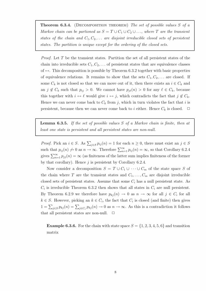
Example 6.3.6. For the chain with state space S = 1, 2, 3, 4, 5, 6 and transition
matrix
8

P =
1/2 1/2 0 0 0 0
1/4 3/4 0 0 0 0
1/4 1/4 1/4 1/4 0 0
1/4 0 1/4 1/4 0 1/4
0 0 0 0 1/2 1/2
0 0 0 0 1/2 1/2
we have S = T ∪C1 ∪C2, where T = 3, 4 are transient aperiodic states and C1
and C2 are irreducible closed sets of ergodic states. #
6.4 Stationary distributions and the limit theorem
Definition 6.4.1. A row matrix π is a stationary distribution for a Markov chain
X if π is a probability distribution on the integers such that πP = π.
Proposition. If µ(m) = π then µ(m+n) = π for all n ≥ 0.
Proof. µ(m+n) = µ(m)P n = µ(m)P P n−1 = π P n = π P n−1 = . . . = π. 2
Theorem 6.4.3. An irreducible chain has a stationary distribution π if and only if
all states are non-null persistent. In that case πi = 1/µi for each state i.
Proof. Omitted! 2
Example 6.1.12. (continued) The Bernoulli process is clearly irreducible and
non-null persistent. We want to find the expectation ETi of the time Ti =
infn ≥ 1 : Xn = i it takes to the state i ∈ 1, . . . , 9, given that X0 = 0. To
that end we note that ETi = µi− 1 where µi is the mean reccurance time for
the modified chain with state space 0, . . . , i and transistion matrix
P =
1−p p 0 · · · 0 0
0 1−p p · · · 0 0
0 0 1−p · · · 0 0...
......
. . ....
...
0 0 0 · · · 1−p p
1 0 0 · · · 0 0
.
As µi = 1/πi (where π refers to the modified chain), we can determine µi by
determining π. This in turn is done by solving the equation
9

π P = π ≡
(1−p) π0 + πi = π0,
p πk−1 + (1−p) πk = πk for k = 1, . . . , i−1,
p πi−1 = πi,
which boils down to
p πk−1 = p πk for k = 1, . . . , i−1 and p π0 = p πi−1 = πi.
Hence we have
π = (π0 · · · π0 p π0) =( 1
i+ p· · · 1
i+ p
p
i+ p
)
,
giving
ETi = µi =i+ p
p− 1 =
i
p.
It should be noted that this result can be established in an entirely different way
making use of the fact that the waiting time in each state before transition to
the next state for the Bernoulli process is geometrically distributed with expected
value 1/p. #
Theorem 6.4.17. For an irreducible aperiodic chain we have pij(n) → 1/µj as
n→∞ for all states i and j.
Proof. Omitted! 2
10

Lecture 3, Thursday 28 January
6.8 Birth processes and the Poisson process
This section belongs to the course but is covered by the treatment of Section 6.9.
6.9 Continuous-time Markov chains
Definition 6.9.1. A family of integer valued random variables X = X(t)t≥0 de-
fined on a common probability space is a Markov chain if
P
X(tn+1) = in+1
∣
∣X(tn) = in, . . . , X(t1) = i1
= PX(tn+1) = in+1|X(tn) = in
for all 0≤ t1 ≤ . . . ≤ tn ≤ tn+1 and i1, . . . , in+1 ∈ Z.
A continuous-time Markov chain may take values in any countable state space,
but when developing the theory it is enough to let the state space be the integers.
Definition. A Markov chain X(t)t≥0 is (time) homogeneous if
PX(t+s) = j |X(s) = i = PX(t) = j |X(0) = i
does not depend on s≥ 0 but only on t≥ 0 for all i, j ∈ Z.
We will (unless otherwise is explicitely stated) only deal with homogeneous Markov
chains. Thus Markov chain will mean homogeneous Markov chain for us in the sequel.
Definition 6.9.2. The transition matrices Ptt≥0 = (pij(t))t≥0 of a (homoge-
neous) Markov chain X(t)t≥0 is made up of the transition probabilities
pij(t) = PX(t+s) = j |X(s) = i = PX(t) = j |X(0) = i
for s, t≥ 0 and i, j ∈Z.
Theorem 6.9.3. The family of transition matrices Ptt≥0 is a stochastic semigroup,
which is to say that
(a) P0 = I (the identity matrix);
(b) Pt is a stochastic matrix (cf. Theorem 6.1.5), which is to say that all pij(t) ≥ 0
and∑
j pij(t) = 1 for all i∈ Z and t≥ 0;
(c) the Chapman-Kolmogorov equations Ps+t = PsPt holds for s, t≥ 0.
11

Proof. The properties (a) and (b) are immediate, while the property (c) follows as
(cf. the proof of Theorem 6.1.7)
(Ps+t)ij = PX(s+t) = j |X(0) = i=∑
k
PX(s+t) = j, X(s) = k |X(0) = i
=∑
k
PX(s+t) = j, X(s) = k, X(0) = iPX(s) = k, X(0) = i
PX(s) = k, X(0) = iPX(0) = i
=∑
k
pkj(t) pik(s)
= (PsPt)ij . 2
We will henceforth assume that the transition semigroup Ptt≥0 is element wise
differentiable from the right at t = 0. The corresponing matrix of derivatives
G = limt↓0
Pt − I
t
is called the generator of the continuous-time Markov chain and takes over the role
of the transition matrix P for discrete-time chains.
Theorem 6.9.5. We may express Pt = (pij(t)) in terms of the generator G = (gij)
as
pij(h) =
gijh + o(h) as h ↓ 0 for i 6= j,
1 + gjjh + o(h) as h ↓ 0 for i = j.
Proof. This is just another way to phrase the fact that G = limt↓0(Pt − I)/t. 2
Note that we must have
gij ≥ 0 for i 6= j while gjj ≤ 0 .
Furthermore, the following formal calculation
1 =∑
j
pij(h) = 1 + gjjh + o(h) +∑
j 6=i
(
gijh + o(h))
= 1 +(∑
j
gij
)
h + o(h)
gives∑
j
gij = 0 .
However, occasionally this formula may fail, which is explained by the fact that
the formal calculation uses a change of order of limit operation that might not be
correct when o(h) is moved outside the sum. We will resolve this issue by restricting
our attention to continuous-time Markov chains for which the above kind of formal
arguments apply (which happens to be the case for virtually all chains of any interest).
12
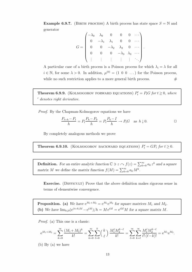
Example 6.9.7. (Birth process) A birth process has state space S = N and
generator
G =
−λ0 λ0 0 0 0 · · ·0 −λ1 λ1 0 0 · · ·0 0 −λ2 λ2 0 · · ·0 0 0 −λ3 λ3 · · ·...
......
......
. . .
.
A particular case of a birth process is a Poisson process for which λi = λ for all
i ∈ N, for some λ > 0. In addition, µ(0) = (1 0 0 . . . ) for the Poisson process,
while no such restriction applies to a more general birth process. #
Theorem 6.9.9. (Kolmogorov forward equations) P ′t = PtG for t≥ 0, where
′ denotes right derivative.
Proof. By the Chapman-Kolmogorov equations we have
Pt+h−Pt
h= Pt
Ph−P0
h= Pt
Ph− I
h→ PtG as h ↓ 0. 2
By completely analogous methods we prove
Theorem 6.9.10. (Kolmogorov backward equations) P ′t = GPt for t≥ 0.
Definition. For an entire analytic function C ∋ z y f(z) =∑∞
k=0 ak zk and a square
matrix M we define the matrix function f(M) =∑∞
k=0 ak Mk.
Exercise. (Difficult) Prove that the above definition makes rigorous sense in
terms of elementwise convergence.
Proposition. (a) We have eM1+M2 = eM1eM2 for square matrices M1 and M2.
(b) We have limh↓0(e(t+h)M− etM )/h = M etM = etMM for a square matrix M .
Proof. (a) This one is a classic:
eM1+M2 =
∞∑
k=0
(M1+M2)k
k!=
∞∑
k=0
k∑
ℓ=0
( k
ℓ
)M ℓ1M
k−ℓ2
k!=
∞∑
ℓ=0
∞∑
k=ℓ
M ℓ1M
k−ℓ2
ℓ! (ℓ−k)!= eM1eM2.
(b) By (a) we have
13

e(t+h)M− etM
h=
e(h+t)M − etM
h=
etM (ehM− I)
h=
(ehM− I) etM
h→ etMM = M etM
as h ↓ 0 since (ehM − I)/h =∑∞
k=1 hk−1Mk/k!. 2
Theorem 6.9.12. Pt = etG for t≥ 0.
Proof. By the Kolmogorov backward equations and the above proposition we have
0 = P ′t −GPt = etG d
dte−tGPt =⇒ d
dte−tGPt = 0 =⇒ e−tGPt = I =⇒ Pt = etG. 2
In view of Theorem 6.9.12 a continuous-time Markov chain is completely specified
by (the state space,) the start distribution µ0) together with the generator G, recall
Example 6.9.7.
Theorem 6.9.13. The time Ti = inft > 0 : X(t) 6= i |X(0) = i spent in state i for
a continuous-time Markov chain is exponetially distributed with parameter −gii.
Proof. For the non-increasing function
f(t) = PX(r) = i for r ∈ (0, t] |X(0) = i
the Markov property and time homogenity give
f(t+s)
f(s)=
PX(r) = i for r ∈ (0, t+s] |X(0) = iPX(r) = i for r ∈ (0, s] |X(0) = i
=PX(r) = i for r ∈ [0, t+s]PX(r) = i for r ∈ [0, s]
= P
X(r) = i for r ∈ (s, t+s]∣
∣X(r) = i for r ∈ [0, s]
= PX(r) = i for r ∈ (s, t+s]|X(s) = i= f(t) for s, t≥ 0.
Hence the non-decreasing function g(t) = − log(f(t)) satisfies the so called Cauchy
functional equation g(t+s) = g(t) + g(s) for s, t≥ 0, the only solutions of which take
the form g(t) = C t for some constant C ∈R.
Now note that for small h > 0 and a grid 0 = h0 < h1 < . . . < hn = h such that
max1≤i≤n hi−hi−1 → 0 as n→∞ we have
PX(r) = i for r ∈ (0, h] |X(0) = i ← P
∩ni=1 X(hi) = i
∣
∣X(0) = i
=n∏
i=1
pii(hi−hi−1)
14
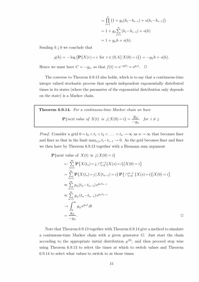
=n∏
i=1
(
1 + gii(hi−hi−1) + o(hi−hi−1))
= 1 + gii
n∑
i=1
(hi−hi−1) + o(h)
= 1 + giih + o(h).
Sending h ↓ 0 we conclude that
g(h) = − log(
PX(r) = i for r ∈ (0, h] |X(0) = i)
= −giih + o(h).
Hence we must have C = −gii, so that f(t) = e−g(t) = egiit. 2
The converse to Theorem 6.9.13 also holds, which is to say that a continuous-time
integer valued stochastic process that spends independent exponentially distributed
times in its states (where the parameter of the exponential distribution only depends
on the state) is a Markov chain.
Theorem 6.9.14. For a continuous-time Markov chain we have
Pnext value of X(t) is j |X(0) = i =gij
−giifor i 6= j.
Proof. Consider a grid 0 = t0 < t1 < t2 < . . . < tn→∞ as n→∞ that becomes finer
and finer so that in the limit maxi≥1 ti−ti−1 → 0. As the grid becomes finer and finer
we then have by Theorem 6.9.13 together with a Riemann sum argument
Pnext value of X(t) is j |X(0) = i
←∞∑
n=1
P
X(tn)=j,∩n−1i=0 X(s)= i
∣
∣X(0) = i
=∞∑
n=1
PX(tn)=j |X(tn−1) = iP
∩n−1i=0 X(s)= i
∣
∣X(0) = i
≈∞∑
n=1
pij(tn−tn−1) egiitn−1
≈∞∑
n=1
gij (tn−tn−1) egiitn−1
→∫ ∞
0
gij egiit dt
=gij
−gii. 2
Note that Theorem 6.9.13 together with Theorem 6.9.14 give a method to simulate
a continuous-time Markov chain with a given generator G: Just start the chain
according to the appropriate initial distribution µ(0), and then proceed step wise
using Theorem 6.9.13 to selcet the times at which to switch values and Theorem
6.9.14 to select what values to switch to at those times.
15
Example. Consider a reliability system consisting of two iid. components with
exponentially distributed life times with parameter λ > 0. The system is started
at time t = 0 with two functioning components X(0) = 2. Then there is a
waiting time equals the minimum of two iid. exponentially distributed life times
with parameter λ, which is to say an exponentially distributed random waiting
time with parameter 2λ, until the system changes to one functioning component
X(t) = 1. Then, by the lack of memory proprty for exponential distributions, there
is a final exponentially distributed random waiting time with parameter λ until
the system changes to its terminal state with no functioning components X(t) = 0.
The process has state space S = 0, 1, 2, starting distribution µ(0) = (0 0 1) and
generator
G =
0 0 0
λ −λ 0
0 2λ −2λ
. #
Definition 6.9.17. A continuous-time Markov chain is irreducible if pij(t) > 0 for
some t≥ 0 for every pair of states i, j.
Theorem 6.9.16. For an irreducible chain we have pij(t) > 0 for all t > 0 for every
pair of states i, j.
Proof. By Theorem 6.9.13 we have
pii(t) ≥ PX(r) = i for r ∈ (0, t] |X(0) = i = egiit > 0
for some t > 0. Now, as the chain is irreducible we have pij(t) > 0 for some t > 0
for i 6= j (since pij(0) = 0). Hence Theorem 6.9.13 shows that there must exist states
i 6= k1 6= . . . 6= kn 6= j such that gik1, gk1k2
, . . . , gknj > 0. For all sufficiently small h > 0
we therefore have pij((n+1)h) ≈ gik1h gk1k2
h · . . . · gknjh > 0. From this in turn we get
pij(t) ≥ pij((n+1)h) pjj(t− (n+1)h) for all t > 0 (picking h > 0 samll enough). 2
Definition 6.9.18. A row matrix π is a stationary distribution for a continuous-
time Markov chain if πPt = π for all t≥ 0.
Theorem 6.9.19. A row matrix π is a stationary distribution if and only if πG = 0.
Proof. We have πPt =∑∞
k=0 πtkGk/k! = π if πG = 0. If on the other hand πPt = π
16

for all t ≥ 0, then we must have∑∞
k=1 πtkGk/k! = 0 for all t ≥ 0, which can only
happen (e.g, by differetiating at t = 0) if πG = 0. 2
We have the following important continuous-time version of the discrete-time limit
Theorem 6.4.17:
Theorem 6.9.21. For an irreducible chain we have limt→∞ pij(t) = πj for all states i
and j if there exists a stationary distribution π. Otherwise we have limt→∞ pij(t) = 0
for all states i and j.
Proof. Omitted! 2
6.11 Birth-death processes (but no imbedding)
Example. (Birth-death process) A birth-death process is the general form of
a continuous-time Markov chain with state space S = N that can only change its
values one unit at a time (upwards or downwards). In other words the generator
is given by
G =
−λ0 λ0 0 0 0 · · ·µ1 −(λ1+µ1) λ1 0 0 · · ·0 µ2 −(λ2+µ2) λ2 0 · · ·0 0 µ3 −(λ3+µ3) λ3 · · ·...
......
......
. . .
. #
Example 6.11.6. (Simple death with immigration) A birth-death process
with death rate µi = i µ proportional to the current state i and constant birth
rate λi = λ. #
Example. To find the stationary distribution π for a birth-death process (if it
exists) we use Theorem 6.9.19 and note that the equation π G = 0 takes the form
−π0λ0 + π1µ1 = 0
πi−1λi−1−πi(µi+λi)+πi+1λi+1 = 0 for i≥ 1⇔ πi =
λ0 . . . λi−1
µ1 . . . µi
π0 for i≥ 1.
We see that this solution is a probability distribution if and only if
∞∑
i=1
λ0 . . . λi−1
µ1 . . . µi<∞ and π0 = 1
/(
1 +
∞∑
i=1
λ0 . . . λi−1
µ1 . . . µi
)
. #
17

Example 6.11.6. (Continued) For the birth-death process with simple death
and immigration we have the stationary distribution is Poisson distributed with
parameter λ/µ. #
18

Lecture 4, Friday 29 January
Chapter 8 Random processes
8.1 Introduction
Definition. Given a sample space Ω a stochastic process X = X(t)t∈T with
parameter set T is a function X : Ω×T → R such that X( · , t) : Ω→ R is a random
variable for each t∈T .
Note that all memebers X(t), t ∈ T , of a stochastic process should be random
variables defined on a common sample space.
The dependence of ω ∈ Ω for a stochastic process X is usually supressed in the
notation (as we did already in the definition), so that we write X(t) or X(t)t∈T
instead of X(ω, t) or X(ω, t)(ω,t)∈Ω×T .
It is natural to belive that a stochastic process is more or less “determined” by its
univariate marginal distributions FX(t)(x) = PX(t)≤ x for x ∈ R, for each t ∈ T .
But this is not true at all as the following exercise demonstrates:
Exercise. Consider the stochastic process X(t) = ξ for t∈R, where ξ is a single
standard normal N(0, 1) distributed random variable. Let Y (t) be a stochastic
process that is N(0, 1) distributed at each t∈R, but with all random values of the
process at different times independent of each other. Find the univariate marginal
distributions FX(t) and FY (t). Pick a “typical” ω ∈ Ω and, for that choice of ω,
plot a likely appearance of the graphs, the so called realisations,
R ∋ t y X(t) = X(ω, t)∈R and R ∋ t y Y (t) = Y (ω, t)∈R.
The univariate marginal distributions do not give any information at all about the
dependence structure of the process at hand. To get such information we consider
Definition. The finite dimensional distributions (fidi’s) FX(t1),...,X(tn) : t1, . . . , tn ∈T, n ∈N of a stochastic process X(t)t∈T are given by
FX(t1),...,X(tn)(x1, . . . , xn) = PX(t1)≤ x1, . . . , X(tn)≤ xn for x1, . . . , xn ∈R.
Although the fidi’s of a process usually offer sufficient information about the
process for probabilistic analysis, it might happen that not even all this information
is sufficient as the following exercise demonstrates:
19

Exercise. Find two stochastic processes X(t)t∈[0,1] and Y (t)t∈[0,1] that have
common fidi’s but that satisfy
PX(t) 6= Y (t) for some t∈ [0, 1] = 1.
8.2 Stationary processes
Definition 8.2.1. A stochastic process X(t)t∈T with T ⊆R is strongly stationary
if(
X(t1+h), . . . , X(tn+h))
=D
(
X(t1), . . . , X(tn))
for all t1+h, . . . , tn+h, t1, . . . , tn ∈ T (where =D denotes equality of distributions).
Definition 8.2.2. A stochastic process X(t)t∈T with T ⊆ R is weakly stationary
if the function T ∋ t y EX(t) is a (finite) constant and if the function T ×T ∋(s, t) y CovX(s), X(t) (is finite and) only depends on the difference t−s between
s and t.
Grimmett and Stirzaker adopt the practice to understand stationary (without any
additional information) as weakly stationary. In doing so they go against common
practice which instead is to understand stationary as strongly stationary. However,
as we use their book we have to follow their practice ...
Example 8.2.8. An iid. sequence of random variables Xnn∈Z is quite obviously
strongly stationary. #
Exercise. Show that strongly stationary processes are stationary when their
expectations and covariances are well-defined.
Exercise. Exemplify that strongly stationary processes need not necessarily be
stationary.
Exercise. Exemplify that stationary processes need not necessarily be strongly
stationary.
Example 8.2.4. A continuous-time Markov chain that has stationary distribu-
tion π is strongly stationary if µ(0) = π. This is so since we then have µ(h) = π
for all h≥ 0, so that
P
X(t1+h)≤ x1, . . . , X(tn+h)≤ xn
20

=∑
k
P
X(t1+h)≤ x1, . . . , X(tn+h)≤ xn
∣
∣X(h) = k
µ(h)k
=∑
k
∑
k1≤x1
· · ·∑
kn≤xn
pkk1(t1) pk1k2
(t2−t1) · . . . · pkn−1kn(tn−tn−1) πk,
where the right-hand side does not depend on h≥ 0. #
Example 8.2.5. For A and B uncorrelated zero-mean unit variance random
variables and λ ∈R a constant the cosine process
X(t) = A cos(λt) + B sin(λt), t∈R,
is stationary since EX(t) = 0 is a constant and
CovX(s), X(t) = VarA cos(λs) cos(λt)
+ CovA, B cos(λs) sin(λt)
+ CovB, A sin(λs) cos(λt)
+ VarB sin(λs) sin(λt)
= cos(λs) cos(λt) + sin(λs) sin(λt)
= cos(λ(t−s))
only depends on the difference t−s between s and t. #
8.3 Renewal processes
Definition 8.3.3. A renewal process N = N(t)t≥0 is given by
N(t) = maxn∈N : Tn ≤ t for t≥ 0,
where Tn =∑n
i=1 Xi and Xi∞i=1 is an iid. sequence of non-negative random variables.
Example 8.3.1. A room is lit by a single light bulb with a random life time X1.
When the bulb fails it is replaced immediately with an iid. copy with life time X2,
and so on . . . . Then Tn =∑n
i=1 Xi is the time to failure of the n-th bulb, and
the renewal process N(t) = maxn∈N : Tn ≤ t is the number of bulbs that have
failed up to time t. #
Example. A renewal process is a Poisson process if and only if the Xi’s are ex-
ponentially distributed. #
Example 8.3.2. Let Yn∞n=0 be a discrete-time Markov chain with Y0 = i for
21

some non-random i∈ Z and define T0 = 0 and
Tn = infn > Tn−1 : Yn = i for n≥ 1.
Then Xn = Tn− Tn−1, n ≥ 1, are iid. non-negative random variables so that the
number of revisits N(t) = maxn∈N : Tn ≤ t to the state i up to time t is a re-
newal process. #
Theorem 8.3.5. A renewal process is a Markov chain if and only if it is a Poisson
process.
Proof. This is Exercise 8.3.5. 2
8.4 Queues
A queue process Q(t)t≥0 counts the total number of customers in a queuing system
at time t≥ 0. The probabilistic behaviour of the queue process will depend on factors
such as
• in what manner do customers arrive to the queuing system?
• what is the queuing disciplin for customers that have arrived to the queue and
are waiting to be served?
• how long are service times for customers?
The simplest kind of queues are birth-and-death continuous-time Markov process.
More complicated queues, albeit not Markov, may be analyzed through an imbedded
discrete-time Markov chain. The most complicated queues are more complicated still.
8.5 The Wiener process
Definition. A Levy7 process is a stochastic process X(t)t≥0 with X(0) = 0 such
that
X(t1)−X(t0), . . . , X(tn)−X(tn−1) are independent random variables
for 0≤ t0 < t1 < . . . < tn−1 < tn, that is, independent increments, and
the distribution of X(t+s)−X(s) does not depend on s≥ 0 but only on t≥ 0,
that is, stationary increments.
7Paul Pierre Levy 1886-1971, very important French probabilist.
22

Definition. A Levy process W (t)t≥0 the increments W (t+s)−W (s) of which are
zero-mean normal distributed is called a Wiener8 process or Brown9ian motion.
The Wiener process is the most important stochastic process in the world.
Theorem. The vector of process values (W (t1), . . . , W (tn)) of a Wiener process has
a zero-mean multivariate normal distribution with covariance matrix
CovW (ti), W (tj) = VarW (1)minti, tj for i, j = 1, . . . , n.
Proof. Assume without loss of generality that 0 ≤ t1 ≤ . . . ≤ tn. We have to check
that the linear combination∑n
i=1 aiW (ti) is univariate normal distributed for any
choice of constants a1, . . . , an ∈R. To that end we note that
n∑
i=1
aiW (ti) =n∑
i=1
( n∑
j=i
aj
)
(W (ti)−W (ti−1)),
where t0 = 0. As the increments of W are independent normal distributed it follows
from elementary properties of the normal distribution that the linear combination∑n
i=1 aiW (ti) is univariate normal distributed.
As W (0) = 0 the fact that increments are zero-mean implies that all process values
W (ti) = (W (ti+0)−W (0)) + W (0) are zero-mean. As for covariances, independence
and stationarity of increments give
CovW (s), W (s+t) = CovW (s), W (s)+ CovW (s), W (s+t)−W (s)= VarW (s)+ 0 for s, t≥ 0.
Here independence and stationarity of increments give
VarW (s+t)= VarW (s+t)−W (t)+ 2CovW (s+t)−W (t), W (t)+ VarW (t)= VarW (s)+ VarW (t) for s, t≥ 0.
We see that f(t) = VarW (t), t≥ 0, is a non-decreasing function of t that solves the
Cauchy functional equation f(s+t) = f(s) + f(t) for s, t≥ 0. However, recalling the
proof of Theorem 6.9.13, the only possible solutions to this equation are f(t) = C t
for some constant C ∈R. In our case that constant must be C = VarW (1). 2
8Norbert Wiener, American scientist 1894-1964 who gave important contributions to mathematics as
well as many other areas of science including early computer science.
9Robert Brown 1773-1858, Scottish botanist who made the first empirical observations of Brownian
motion as the movement pattern of small particles in a fluid.
23

24
Lecture 5, Thursday 4 February
Chapter 9 Stationary processes
9.1 Introduction
Recall Definitions 8.2.1 and 8.2.2 of strong stationarity and (weak) stationarity, re-
spectively.
In this chapter it will sometimes be natural to consider complex valued stochastic
processes: A complex valued stochastic process is a family X(t)t∈T of complex
valued random variables defined on a common sample space Ω. A complex valued
random variable X, in turn, simply is a function X : Ω→C. Eqivalently, a complex
valued random variable X is given by X = X1 + iX2, where the real and imaginary
part of X, X1 and X2, respectively, are ordinary real valued random variables.
The Definition 8.2.1 of strong stationarity that
(
X(t1+h), . . . , X(tn+h))
=D
(
X(t1), . . . , X(tn))
for all t1 +h, . . . , tn +h, t1, . . . , tn ∈ T formally remains valid for a complex valued
process X(t)t∈T . Now the above equality in distribution =D simply means that
P
X(t1+h)∈A1, . . . , X(tn+h) ∈An
= P
X(t1) ∈A1, . . . , X(tn) ∈An
for all subsets A1, . . . , An of C.
The expected value of a complex valued random variable X = X1 + iX2 with real
and imaginary part X1 and X2, respectively, is defined EX = EX1+ iEX2.
Definition 9.1.1. The covariance between two complex valued random variables X
and Y defined on a common probability space is given by
CovX, Y = E
(
X−EX) (
Y −EY )
.
Having resolved the of issue how to define expectations and covariaces for complex
valued random variables, the Definition 8.2.2 of (weak) stationarity that the function
T ∋ t y EX(t) is a constant and that the function T ×T ∋ (s, t) y CovX(s),
X(t) only depends on the difference t−s between s and t remains valid for a complex
valued process X(t)t∈T .
Definition 9.1.2. The variance of a complex valued random variable X is given by
VarX = CovX, X.
25

Definition 9.1.3. Two complex valued random variables X and Y are orthogonal if
CovX, Y = 0.
Example 9.1.4. Pick an integer m ≥ 2 and let X(t) = e2πi(Z+N(t))/m, where
N(t)t≥0 is a Poisson process with intensity λ > 0 and Z is a random variable
that is independent of N and uniformly distributed over the integers 1, . . . , m.By symmetry considerations it is clear that EX(t) = 0. Further, we have
CovX(t), X(t+h) = E
X(t) X(t+h)
= E
e2πi(N(t)−N(t+h))/m
= E
e−2πi N(h)/m
= e−λh(1+2πi/m) for h≥ 0
(by basic properties of Poisson processes and elementary calculations), so that X is
stationary with covariance CovX(t), X(t+h) = e−λ|h|−2πiλh/m) for h∈R, see the
following exercise. #
Exercise. Explain how the formula CovX(t), X(t+h) = e−λ|h|−2πiλh/m) for
h∈R in Example 9.1.4 follows from the fact that the formula holds for h≥ 0.
9.2 Linear prediction
Theorem 7.9.17. Given random variables X1, . . . , Xn and a square-integrable ran-
dom variable Y , the function φ : Rn→R that minimizes the mean-square prediction
error
E
[Y −φ(X1, . . . , Xn)]2
is given by the minimum mean-square error predictor
φ(x1, . . . , xn) = E
Y∣
∣X1 =x1, . . . , Xn =xn
.
Proof. For the linear space H of square-integrable functions h(X1, . . . , Xn) we have
E
[Y −φ(X1, . . . , Xn)]Z
= E
E
[Y −φ(X1, . . . , Xn)]Z∣
∣X1, . . . , Xn
= E
E
Y −φ(X1, . . . , Xn)∣
∣X1, . . . , Xn
Z
= E
[
E
Y∣
∣X1, . . . , Xn
− E
Y∣
∣X1, . . . , Xn
]
Z
= 0 for Z ∈H.
26

From this in turn it follows that
E
[Y −Z]2
= E
[Y −φ(X1, . . . , Xn)]2
+ 2E
[Y −φ(X1, . . . , Xn)] [φ(X1, . . . , Xn)−Z]
+ E
[φ(X1, . . . , Xn)−Z]2
= E
[Y −φ(X1, . . . , Xn)]2
+ E
[φ(X1, . . . , Xn)−Z]2
≥ E
[Y −φ(X1, . . . , Xn)]2
for any Z ∈H. 2
Given the information about the values of the random variables X1, . . . , Xn, the
minimum mean-square error predictor of the random variable Y is given by Theorem
7.9.17. However, the actual evaluation of that predictor as a rule requires knowledge
about the joint distribution of (Y, X1, . . . , Xn), which is usually not available in a
typical statistical application. In practice, one therefore often instead employ the
following alternative predictor which only requires knowledge about the covariance
structure between the random variables Y, X1, . . . , Xn:
Theorem 9.2.1. Given square-integrable random variables X1, . . . , Xn and Y , the
linear function (x1, . . . , xn) ∋ Rn y∑n
i=1 aixi → R that minimizes the mean-square
prediction error
E
[Y −∑n
i=1aiXi]2
is given by the minimum mean-square error linear predictor for which aini=1 satisfy
EXiY =∑n
j=1 aj EXiXj for i = 1, . . . , n.
In particular, if the random variables X1, . . . , Xn are zero-mean, then
CovXi, Y =∑n
j=1 aj CovXi, Xj for i = 1, . . . , n.
Proof. The idea of the proof is the same as that in the proof of Theorem 7.9.17: For
any linear predictor∑n
j=1 biXi we have
E
[Y −∑n
j=1ajXj]∑n
i=1biXi
=n∑
i=1
bi
(
EXiY −∑n
j=1aj EXiXj)
= 0,
so that
E
[Y −∑n
i=1biXi]2
= E
[Y −∑n
j=1ajXj ]2
+ 2E
[Y −∑n
j=1ajXj ]∑n
i=1(ai−bi)Xi
+ E
[∑n
i=1(ai−bi)Xi]2
= E
[Y −∑nj=1ajXj ]
2
+ E
[∑n
i=1(ai−bi)Xi]2
≥ E
[Y −∑n
j=1ajXj ]2
. 2
27

Example 9.2.5. (Autoregressive scheme) Let Znn∈Z be a sequence of
independent zero-mean random variables with common variances σ2. Let Xnn∈Z
be a stationary so called AR-process such that for some constant α∈ (−1, 1)
Zn is independent of Xn−1, Xn−2, . . . for n ∈Z,
Xn = α Xn−1 + Zn for n ∈Z.
Then stationarity gives
EXn = αEXn−1+ EZn = α EXn+ 0 =⇒ EXn = 0,
while the autocovariance function (see the next definition below) is given by
c(k) ≡ CovXn−k, Xn = CovXn−k, α Xn−1 + Zn = α c(k−1) + 0 for k ≥ 1,
so that c(k) = c(0) α|k| for k ∈Z. Here stationarity gives
c(0) = VarXn = Varα Xn−1+Zn = α2 VarXn−1+VarZn = α2 c(0)+σ2,
so that
c(k) =σ2
1−α2α|k| for k ∈Z.
Hence Theorem 9.2.1 shows that the minimum mean-square error linear predictor∑n
i=1 aiXi of Xn+k is given by the equations
CovXi, Xn+k =∑n
j=1 aj CovXi, Xj for i = 1, . . . , n,
which is to say that
αn+k−i =∑n
j=1 aj α|j−i| for i = 1, . . . , n.
This system of equations is solved by a1 = . . . = an−1 = 0 and an = αk. #
9.3 Autocovariances and spectra
Definition. The autocovariance function c of a complex valued (weakly) stationary
process X = X(t)t∈T is defined as
c(t) = CovX(s), X(s+t) for s, s+t∈ T.
When considering stationary processes we will henceforth assume (unless other-
wise is explicitely stated) that the (constant) expected value of the process is zero, as
28
that only amounts to a shift of a constant level as compared with the general case.
Theorem 9.3.2. The autocovariance function c of a complex valued stationary pro-
cess X = X(t)t∈T is hermitian, which is to say that
c(−t) = c(t) for all t,
and non-negative definite, which is to say that
n∑
i,j=1
c(ti−tj) zizj ≥ 0 for all n ∈N, z1, . . . , zn ∈C and t1, . . . , tn ∈ T.
Proof. By Definition 9.1.1 we have
c(−t) = CovX(s), X(s−t) = CovX(s+t), X(s) = CovX(s), X(s+t) = c(t),
while Definition 9.1.2 gives
0 ≤ Var
n∑
i=1
ziX(ti)
= Cov
n∑
i=1
ziX(ti),n∑
j=1
zjX(tj)
=n∑
i,j=1
c(ti−tj) zizj . 2
Definition 9.3.3. The autocorrelation function ρ of a complex valued stationary
process X = X(t)t∈T is defined as
ρ(t) =CovX(s), X(s+t)
√
VarX(s)VarX(s+t)=
c(t)
c(0)for s, s+t∈ T
whenever c(0) > 0.
The following important theorem is given without proof because the proof belongs
to a course in advanced calculus (in particular Fourier transforms) and do not have
any probabilistic content:
Theorem 9.3.4. (Spectral theorem for autocorrelations) If a stationary
process has variance c(0) > 0 and autocorrelation function ρ(t) that is continuous at
t = 0, then there exists a probability distribution function F , the so called spectral
distribution function of the process, such that ρ is the characteristic function of F ,
which is to say that
ρ(t) =
∫ ∞
−∞
eitλ dF (λ) for all t.
Proof. Omitted. 2
The interpretation of the spectral representation of the autocorrelation function
29

is just the usual one of Fourier transforms as the build up of the autocorrelation
function by means of its frequency content.
The integral in the spectral representation is a so called Riemann-Stieltjes integral
which is obtained as the limit of approximating Riemann-Stieltjes sums∫ ∞
−∞
eitλ dF (λ) = limmax
n(λn−λn−1)↓0
∑
n
eitλn−1(
F (λn)−F (λn−1))
as the mesh −∞← . . . < λ−2 < λ−1 < λ0 < λ1 < λ2 . . . →∞ becomes finer and finer.
If the spectral distribution is a continuous distribution with probability density
function f(λ) = F ′(λ), so that
F (λn)−F (λn−1) = (λn−λn−1) f(λn−1) + o(λn−λn−1) as maxn
(λn−λn−1) ↓ 0,
the we have
ρ(t) =
∫ ∞
−∞
eitλ f(λ) dλ for all t,
as a Riemann sum argument shows that∫ ∞
−∞
eitλ dF (λ) = limmax
n(λn−λn−1)↓0
∑
n
eitλn−1(
F (λn)−F (λn−1))
= limmax
n(λn−λn−1)↓0
∑
n
eitλn−1(λn−λn−1) f(λn−1)
=
∫ ∞
−∞
eitλ f(λ) dλ.
In this case we call f the spectral density function of the process.
If X is a real-valued process, then Theorem 9.3.2 shows that ρ is a symmetric
function (as c is). From this we get that the spectral distribution must be a symmetric
distribution, by uniqueness of Fourier-Stieltjes transforms together with the fact that∫ ∞
−∞
eitλ dF (λ) = ρ(t) = ρ(−t) =
∫ ∞
−∞
e−itλ dF (λ) =
∫ ∞
−∞
eitλ dF (−λ).
In this case we may also use the following simplified spectral representation
ρ(t) =ρ(t)+ρ(−t)
2=
∫ ∞
−∞
eitλ +e−itλ
2dF (λ)
=
∫ ∞
−∞
cos(tλ) dF (λ)
= 2
∫ ∞
0
cos(tλ) dF (λ).
Definition 9.3.10. The spectrum of a stationary process with spectral distribution
function F is the set
λ ∈R : F (λ+ε)−F (λ−ε) > 0 for all ε > 0.
30
Remembering the definition of the Riemann-Stieltjes integral as the limit of ap-
proximating Riemann-Stieltjes sums we see that the spectrum simply consists of
those frequencies that contributes to the build up of the autocorrelations function
(by means of its frequencies).
Theorem. For a continuous time stationary process X(t)t∈R possessing an inte-
grable autocorrelation function∫ ∞
−∞
|ρ(t)| dt <∞
that is continuous at zero, we have
ρ(t) =
∫ ∞
−∞
eitλ f(λ) dλ for t ∈R,
where the spectral density function f is given by
f(λ) =1
2π
∫ ∞
−∞
e−itλ ρ(t) dt for λ ∈R.
Proof. This simply is Fourier transform theory. 2
We will return to examples of application of this theorem later, e.g., when we
study Gaussian processes. We will now instead consider discrete time processes.
Theorem. For a discrete time stationary process X(t)t∈Z possesing an autocorre-
lation function ρ that is continuous at zero, we have
ρ(n) =
∫
(−π,π]
eitλ dF (λ) for n∈ Z,
for a spectral distribution function F such that F (−π) = 0 and F (π) = 1.
Proof. Writing G for the spectral distribution function for the process X that is
provided by Theorem 9.3.4, we have
ρ(n) =
∫ ∞
−∞
einλ dG(λ)
=
∞∑
k=−∞
∫
((2k−1)π,(2k+1)π]
einλ dG(λ)
=
∞∑
k=−∞
∫
(−π,π]
ein(λ+2kπ) dG(λ+2kπ)
=
∫
(−π,π]
einλ
(
∞∑
k=−∞
dG(λ+2kπ)
)
. 2
31

Exercise. (Difficult) There is a possible element of “cheating” in the appli-
cation of Theorem 9.3.4 in the above proof – explain what can be the problem!
Theorem 9.3.15. For a discrete time stationary process X(t)t∈Z possesing a
summable autocorrelation function
∞∑
n=−∞
|ρ(n)| <∞
that is continuous at zero, we have
ρ(n) =
∫ π
−π
einλ f(λ) dλ for n∈ Z,
where the spectral density function f is given by
f(λ) =1
2π
∞∑
n=−∞
e−inλ ρ(n) for λ ∈ [−π, π].
Proof. This simply is Fourier series theory. 2
Example 9.3.19. (Disrete time white noise) A sequence Xnn∈Z of un-
correlated zero-mean random variables with unit variance is stationary with au-
tocovariance function and autocorrelation function given by c(n) = ρ(n) = δ(n)
(Kronecker’s10 delta). As ρ is summable the process has spectral density function
f(λ) =1
2π
∞∑
n=−∞
e−inλ ρ(n) =1
2πfor λ ∈ [−π, π]. #
Example 9.3.20. (Identical sequence) A process Xnn∈Z given by Xn = Y
for n ∈Z for a single zero-mean and unit variance random variable Y is stationary
with autocovariance function and autocorrelation function given by c(n) = ρ(n) =
1 for n ∈ Z. This ρ is not summable, but we see that the spectral distribution
function F corresponds to a unit mass at zero as that gives
ρ(n) =
∫
(−π,π]
eitλ dF (λ) = eit·0 = 1 for n∈ Z. #
Example 9.2.5. (continued) The AR-process Xnn∈Z in Example 9.2.5 has
autocorrelation fucntion ρ(n) = α−|n|, so that the spectral density function is
f(λ) =1
2π
∞∑
n=−∞
e−inλ α−|n| = · · · = 1−α2
2π (1+α2−2α cos(λ))for λ ∈ [−π, π]. #
10Leopold Kronecker, German mathematician 1823-1891.
32

Lecture 6, Friday 5 February
9.4 Stochastic integration and the spectral representation
This section is in essence a single very long proof of the so called spectral theorem.
The details of that proof are argubly not terribly important on their own, and they
will therefore be omitted. Also, no hand-in exercise is required for this section.
Theorem 9.4.2. (Spectral theorem) If a stationary process X has autocorrela-
tion function ρ(t) that is continuous at t = 0 with spectral distribution function F ,
then there exists a complex valued zero-mean stochastic process S(λ)λ∈R called the
spectral process of X, that has orthogonal increments, which is to say
Cov
S(λ)−S(µ), S(η)−S(ν)
= 0 for −∞< µ≤ λ≤ ν ≤ η <∞,
and that satisfies
VarS(λ)−S(µ) = F (λ)−F (µ) for −∞< µ≤ λ<∞,
such that X has spectral representation
X(t) =
∫ ∞
−∞
e−itλ dS(λ) for all t.
Proof. Omitted. 2
The stochastic integral∫∞
−∞e−itλ dS(λ) in the spectral representation is a (stochas-
tic) Riemann-Stieltjes integral obtained as the limit
X(t) =
∫ ∞
−∞
e−itλ dS(λ) = limmax
n(λn−λn−1)↓0
∑
n
e−itλn−1(
S(λn)−S(λn−1))
of approximating Riemann-Stieltjes sums as the mesh −∞ ← . . . < λ−2 < λ−1 <
λ0 < λ1 < λ2 . . . →∞ becomes finer and finer, see also the text following Theorem
9.3.4. As we are talking about convergence of random variables here, we must specify
in which sense that convergence is. And that is in mean-square, which is to say that
the convergence displayed in the previous formula really means (by definition) that
limmax
n(λn−λn−1)↓0
E
(
X(t)−∑
n
e−itλn−1(
S(λn)−S(λn−1))
)2
= 0.
Example. The spectral theorem implies the spectral representation in Theorem
9.3.4 of the autocorrelation function, as
ρ(t)
= CovX(s), X(s+t)
33
= limCov
∑
m
e−isλm−1(
S(λm)−S(λm−1))
,∑
n
e−i(s+t)λn−1(
S(λn)−S(λn−1))
= lim∑
m
∑
n
ei(s+t)λn−1−isλm−1Cov
S(λm)−S(λm−1), S(λn)−S(λn−1)
= lim∑
n
eitλn−1 Var
S(λn)−S(λn−1)
= lim∑
n
eitλn−1(
F (λn)−F (λn−1))
=
∫ ∞
−∞
eitλ dF (λ). #
9.5 The ergodic theorem
Also the treatment of this section will be shortened and rather summary. However,
for this section a hand-in exercise is required. (We will instead use our time to give
a rather extensive treatment of Gaussian processes in the next section.)
The strong law of large numbers states that for an iid. sequence of random variables
Xn∞n=1 that are integrable, E|X1| <∞, we have
1
n
n∑
i=1
Xi → EX1 as n→∞.
Here the convergence is strong, which is to say that the sequence on the left-hand
side converges to the limit on the right-hand side for all ω ∈ Ω (or for all ω except
those in an event with probability zero).
Ergodic theorems deal with generalizations of the strong law of large numbers
to sequences of random variables that are strongly or weakly stationary, but not
necessarily iid.
Theorem 9.5.2. (Ergodic theorem for strongly stationary processes)
If Xn∞n=1 is a strongly stationary sequence of random variables that are integrable,
E|X1| <∞, then there exists an integrable random variable Y such that
1
n
n∑
i=1
Xi → Y as n→∞
in the sense of strong convergence (see above) as well as in the sense of mean con-
vergence, which is to say that
E
∣
∣
∣
∣
1
n
n∑
i=1
Xi − Y
∣
∣
∣
∣
→ 0 as n→∞.
Proof. Omitted. 2
34
Theorem 9.5.3. (Ergodic theorem for stationary processes) If Xn∞n=1
is a stationary sequence of random variables, then there exists a square-integrable
random variable Y with EY = EX1 such that
1
n
n∑
i=1
Xi → Y as n→∞
in the sense of mean-square convergence, which is to say that
E
(
1
n
n∑
i=1
Xi − Y
)2
→ 0 as n→∞.
Proof. Omitted. 2
Exercise. Prove that mean-square convergence implies mean convergence.
The following example illustrates the usefulness of ergodicity results:
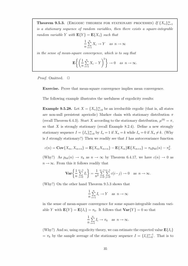
Example 9.5.28. Let X = Xn∞n=0 be an irreducible ergodic (that is, all states
are non-null persistent aperiodic) Markov chain with stationary distribution π
(recall Theorem 6.4.3). Start X according to the stationary distribution, µ(0) = π,
so that X is strongly stationary (recall Example 8.2.4). Define a new strongly
stationary sequence I = In∞n=0 by In = 1 if Xn = k while In = 0 if Xn 6= k. (Why
is I strongly stationary?) Then we readily see that I has autocovariance function
c(n) = CovXm, Xm+n = EXmXm+n − EXmEXm+n = πkpkk(n)− π2k.
(Why?) As pkk(n) → πk as n → ∞ by Theorem 6.4.17, we have c(n) → 0 as
n→∞. From this it follows readily that
Var
1
n
n−1∑
i=0
Ii
=1
n2
n−1∑
i=0
n−1∑
j=0
c(i−j)→ 0 as n→∞.
(Why?) On the other hand Theorem 9.5.3 shows that
1
n
n∑
i=1
Ii → Y as n→∞
in the sense of mean-square convergence for some square-integrable random vari-
able Y with EY = EI1 = πk. It follows that VarY = 0 so that
1
n
n∑
i=1
Ii → πk as n→∞.
(Why?) And so, using ergodicity theory, we can estimate the expected value EI1= πk by the sample average of the stationary sequence I = Iin−1
i=0 . That is to
35

say that we can move along a single sample path of I to estimate an theoret-
ical expected value by means of a smaple average, instead of (as in elementary
statistics) requiring several independent copies of I. #
Exercise. Answer the four whys in Example 9.5.28.
36

Lecture 7, Thursday 11 February
9.6 Gaussian processes
Definition 9.6.3. A stochastic process X(t)t∈T is Gaussian11 if each vector of
process values (X(t1), . . . , X(tn)) is multivariate normal distributed, which is to say,
n∑
i=1
aiX(ti) is univariate normal distributed
for each choice of n∈N and a1, . . . , an ∈R.
By Theorem 9.3.2 the autocovariance function of a real-valued stationary process
X(t)t∈T is symmetric and non-negative definite. This result has the converse that
every symmetric and non-negative definite function is the autocovariance function for
some stationary process. More precisely, we have the following result:
Theorem 9.6.1. If T \T ∋ t y c(t) ∈ R is a symmetric and non-negative definite
function, then there exists a zero-mean stationary Gaussian process X(t)t∈T that
has autocovariance function c.
Proof. The proof of this result is very closely linked to the so called Kolmogorov
Consistency theorem; a result that we have omitted as it goes into the very hart of
Lebesgue measure theory. 2
Example 9.6.13. The treatment of the Wiener process in Section 8.5 shows that
the Wiener process is a Gaussian process. #
It is an immediate consequence of Definition 9.6.3 that each process value X(t) of
a Gaussian process X(t)t∈T is normal distributed (take n = 1, t1 = t and a1 = 1).
However, the converse is not true, which is to say that a process for which each
process value X(t) is normal distributed need not be Gaussian.
Example. Let ξ and η be independent standard normal distributed random vari-
ables and consider the process X = X(t)t∈0,1 defined by X(0) = sign(ξ)η and
X(1) = sign(η)ξ. Then X is not Gaussian albeit X(0) and X(1) are both standard
normal distributed, see Exercise below. #
Exercise. (Difficult) The process in the above example is not Gaussian.
11Johann Carl Friedrich Gauss, German mathematcian 1777-1855. Argubly the greatest mathematician
of all time (albeit, also argubly, an equally distinguished bore).
37
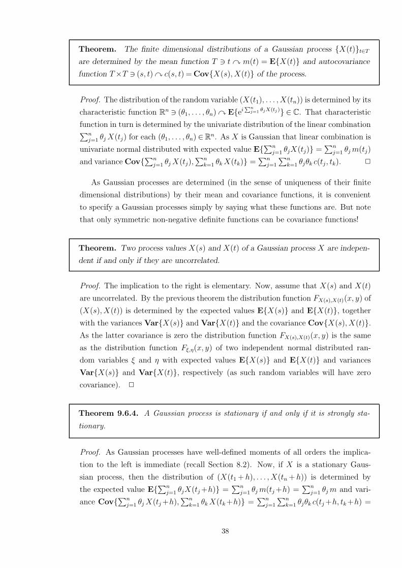
Theorem. The finite dimensional distributions of a Gaussian process X(t)t∈T
are determined by the mean function T ∋ t y m(t) = EX(t) and autocovariance
function T×T ∋ (s, t) y c(s, t) = CovX(s), X(t) of the process.
Proof. The distribution of the random variable (X(t1), . . . , X(tn)) is determined by its
characteristic function Rn ∋ (θ1, . . . , θn) y Eei
Pnj=1
θjX(tj ) ∈ C. That characteristic
function in turn is determined by the univariate distribution of the linear combination∑n
j=1 θj X(tj) for each (θ1, . . . , θn) ∈Rn. As X is Gaussian that linear combination is
univariate normal distributed with expected value E∑n
j=1 θjX(tj) =∑n
j=1 θj m(tj)
and variance Cov∑n
j=1 θj X(tj),∑n
k=1 θk X(tk) =∑n
j=1
∑nk=1 θjθk c(tj , tk). 2
As Gaussian processes are determined (in the sense of uniqueness of their finite
dimensional distributions) by their mean and covariance functions, it is convenient
to specify a Gaussian processes simply by saying what these functions are. But note
that only symmetric non-negative definite functions can be covariance functions!
Theorem. Two process values X(s) and X(t) of a Gaussian process X are indepen-
dent if and only if they are uncorrelated.
Proof. The implication to the right is elementary. Now, assume that X(s) and X(t)
are uncorrelated. By the previous theorem the distribution function FX(s),X(t)(x, y) of
(X(s), X(t)) is determined by the expected values EX(s) and EX(t), together
with the variances VarX(s) and VarX(t) and the covariance CovX(s), X(t).As the latter covariance is zero the distribution function FX(s),X(t)(x, y) is the same
as the distribution function Fξ,η(x, y) of two independent normal distributed ran-
dom variables ξ and η with expected values EX(s) and EX(t) and variances
VarX(s) and VarX(t), respectively (as such random variables will have zero
covariance). 2
Theorem 9.6.4. A Gaussian process is stationary if and only if it is strongly sta-
tionary.
Proof. As Gaussian processes have well-defined moments of all orders the implica-
tion to the left is immediate (recall Section 8.2). Now, if X is a stationary Gaus-
sian process, then the distribution of (X(t1 +h), . . . , X(tn +h)) is determined by
the expected value E∑n
j=1 θjX(tj +h) =∑n
j=1 θj m(tj +h) =∑n
j=1 θj m and vari-
ance Cov∑n
j=1 θj X(tj +h),∑n
k=1 θk X(tk +h) =∑n
j=1
∑nk=1 θjθk c(tj +h, tk +h) =
38
∑nj=1
∑nk=1 θjθk c(tk−tj) for any θ1, . . . , θn ∈ R, see the proof of the theorem on the
top of the previous page. As these quantities do not depend on h the process is
strongly stationary. 2
The above established properties for Gaussian processes are very special and can-
not at all be expected to hold for stochastic processes in general!
Example. If X = Xnn∈N consists of iid. standardized normal distributed ran-
dom variables, then by Example 9.3.19 X is stationary with mean function 0 and
covariance function Kronecker’s delta. This process is Gaussian since∑n
i=1 aiXi
is zero-mean normal distributed with variance∑n
i=1 a2i for a1, . . . , an ∈ R. Hence
(unsurprisingly by Example 8.2.8), X is strongly stationary by Theorem 9.6.4. #
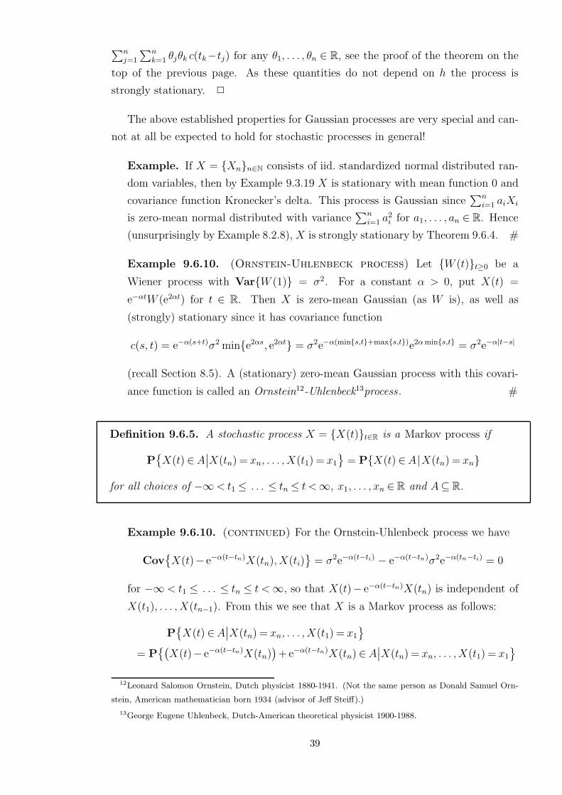
Example 9.6.10. (Ornstein-Uhlenbeck process) Let W (t)t≥0 be a
Wiener process with VarW (1) = σ2. For a constant α > 0, put X(t) =
e−αtW (e2αt) for t ∈ R. Then X is zero-mean Gaussian (as W is), as well as
(strongly) stationary since it has covariance function
c(s, t) = e−α(s+t)σ2 mine2αs, e2αt = σ2e−α(mins,t+maxs,t)e2α mins,t = σ2e−α|t−s|
(recall Section 8.5). A (stationary) zero-mean Gaussian process with this covari-
ance function is called an Ornstein12-Uhlenbeck13process. #
Definition 9.6.5. A stochastic process X = X(t)t∈R is a Markov process if
P
X(t) ∈A∣
∣X(tn) = xn, . . . , X(t1) = x1
= PX(t) ∈A |X(tn) = xn
for all choices of −∞< t1 ≤ . . . ≤ tn ≤ t <∞, x1, . . . , xn ∈R and A⊆R.
Example 9.6.10. (continued) For the Ornstein-Uhlenbeck process we have
Cov
X(t)− e−α(t−tn)X(tn), X(ti)
= σ2e−α(t−ti) − e−α(t−tn)σ2e−α(tn−ti) = 0
for −∞ < t1 ≤ . . . ≤ tn ≤ t <∞, so that X(t)− e−α(t−tn)X(tn) is independent of
X(t1), . . . , X(tn−1). From this we see that X is a Markov process as follows:
P
X(t) ∈A∣
∣X(tn) = xn, . . . , X(t1) = x1
= P(
X(t)− e−α(t−tn)X(tn))
+e−α(t−tn)X(tn) ∈A∣
∣X(tn) = xn, . . . , X(t1) = x1
12Leonard Salomon Ornstein, Dutch physicist 1880-1941. (Not the same person as Donald Samuel Orn-
stein, American mathematician born 1934 (advisor of Jeff Steiff).)
13George Eugene Uhlenbeck, Dutch-American theoretical physicist 1900-1988.
39

= P(
X(t)− e−α(t−tn)X(tn))
+e−α(t−tn)X(tn) ∈A∣
∣X(tn) = xn
= PX(t) ∈A |X(tn) = xn. #
Theorem. A stationary zero-mean Gaussian process X(t)t∈R is Markov if and
only if it is an Ornstein-Uhlenbeck process.
Proof. The implication to the left follows from Example 9.6.10. Conversely, if X is
stationary zero-mean Gaussian with covariance function c, then we have
EX(t+s) |X(s) = y = E
X(t+s)− c(t)
c(0)X(s)
∣
∣
∣
∣
X(s) = y
+c(t)
c(0)y =
c(t)
c(0)y
for t ≥ 0, since X(t+s)− (c(t)/c(0)) X(s) is independent of X(s) (as these random
variables are uncorrelated). If in addition X is Markov, it follows that
c(t+s)
c(0)=
EX(t+s)X(0)c(0)
=1
c(0)
∫ ∞
−∞
∫ ∞
−∞
EX(t+s)X(0) |X(0) = x, X(s) = y dFX(0),X(s)(x, y)
=1
c(0)
∫ ∞
−∞
∫ ∞
−∞
xEX(t+s) |X(s) = y dFX(0),X(s)(x, y)
=c(t)
c(0)2
∫ ∞
−∞
∫ ∞
−∞
xy dFX(0),X(s)(x, y)
=c(t)
c(0)2EX(s)X(0)
=c(t)
c(0)
c(s)
c(0)for s, t≥ 0.
Hence we must have c(t)/c(0) = e−αt for t ≥ 0 for some constant α ≥ 0 (recall The-
orem 6.9.13 and see Exercise below), so that c(t) = c(0) e−α|t| for t ∈R by symmetry
of c. Hence X is an Ornstein-Uhlenbeck process. 2
Exercise. Show that if a stationary stochastic process X(t)t∈R has covariance
function c(t) = c(0) e−α|t| for t ∈ R for some constant α ∈ R, then it must hold
that α≥ 0.
Remeber that you must do two hand-in exercises for this lecture!
40

Lecture 8, Friday 12 February
Chapter 10 Renewals
10.1 The renewal equation
Definition 10.1.1. Given a sequence Xi∞i=1 of iid. non-negative random variables
and writing Tn =∑n
i=1 Xi, a renewal process N = N(t)t≥0 is given by
N(t) = maxn : Tn ≤ t for t≥ 0.
Theorem. We have N(t)≥ n if and only if Tn ≤ t.
Proof. The implication to the left is immediate from Definition 10.1.1. Conversely, if
Tn > t, then Definition 10.1.1 shows that N(t) < n. 2
Theorem 10.1.2. If EX1 > 0 then PN(t) <∞ = 1.
Proof. If EX1 > 0 then PX1≥ δ ≥ ε for some selection of δ, ε > 0, so that
PN(t) < n = PTn > t = 1−PTn≤ t ≥ 1−P
Bin(n, ε)≤ t
δ
→ 1
as n→∞ (see Exercise below). 2
Exercise. Explain the last two steps in the equation in the proof of Theorem
10.1.2.
Henceforth we always assume not only that µ = EX1 is strictly positive (and
finite), but that X1 is strictly positive, which is to say that PX1> 0 = 1.
Example 10.1.15. A Poisson process is a renewal process with X1 exponentially
distributed. Recall from Theorem 8.3.5 that this is the only renewal process that is
a Markov chain. #
Definition. The distribution functions of X1 and Tn are denoted F and Fn, respec-
tively.
Lemma 10.1.4. Fn+1(x) =∫ x
0Fn(x−y) dF (y) for x > 0 and n≥ 1.
41

Proof. We have
Fn+1(x) = PTn+1 ≤ x= PTn+Xn+1 ≤ x
=
∫ x
0
PTn+y ≤ x dF (y)
=
∫ x
0
Fn(x−y) dF (y). 2
Lemma 10.1.5. PN(t) = n = Fn(t)− Fn+1(t) for t > 0 and n≥ 1.
Proof. We have
PN(t) = n = PN(t)≥ n −PN(t)≥ n+1= PTn≤ t −PTn+1 ≤ t= Fn(t)− Fn+1(t). 2
Definition 10.1.6. The renewal function m is given by m(t) = EN(t).
Lemma 10.1.7. m(t) =∑∞
n=1 Fn(t) for t > 0.
Proof. We have
EN(t) =
∞∑
k=1
k PN(t) = k
=∞∑
k=1
k∑
n=1
PN(t) = k
=
∞∑
n=1
∞∑
k=n
PN(t) = k
=
∞∑
n=1
PN(t)≥ n
=
∞∑
n=1
PTn ≤ t
=∞∑
n=1
Fn(t). 2
Lemma 10.1.8. m(t) = F (t) +∫ t
0m(t−x) dF (x) for t > 0.
42

Proof. We have
EN(t) =
∫ ∞
0
EN(t) |X1 =x dF (x)
= 0 +
∫ t
0
EN(t−x)+1 dF (x)
=
∫ t
0
m(t−x) dF (x) + F (t). 2
Lemma 10.1.8 can be expressed in terms of convolution language as
m = F + m ⋆ F .
Definition 10.1.10. Given a bounded function H we call the equation
µ(t) = H(t) +
∫ t
0
µ(t−x) dF (x) for t > 0
a renewal-type equation (where a solution µ is sought after).
Note that the renewal-type equation in Definition 10.1.10 can be expressed as
µ = H + µ ⋆ F .
Theorem 10.1.11. The renewal-type equation in Definition 10.1.10 has solution
µ = H + H ⋆ m.
Proof. As m = F + m ⋆ F by Lemma 10.1.8 it follows that µ = H + H ⋆ m satisfies
µ = H + H ⋆ m = H + H ⋆ (F +m ⋆ F ) = H + (H +H ⋆ m) ⋆ F = H + µ ⋆ F. 2
Example 10.1.15. A Poisson process N(t)t≥0 with intensity λ has expected
value EN(t) = λt. We may recover this result using that N is a renewal
process with X1 exponentially distributed with parameter λ, so that Tn is Γ(n, λ)-
distributed and Lemma 10.1.7 gives
m(t) =∞∑
n=1
PTn ≤ t =∞∑
n=1
∫ t
0
λ (λs)n−1
(n−1)!e−λs ds =
∫ t
0
λ ds = λt. #
10.2 Limit theorems
Theorem 10.2.1. We have N(t)/t→ 1/µ as t→∞.
Proof. By the strong law of large numbers we have∑n
i=1 Xi/n → µ as n→∞. It
43

follows that
N(t)
t=
maxn :∑n
i=1 Xi ≤ tt
= max
n
t:
1
n
n∑
i=1
Xi ≤t
n
→ max
n
t: µ≤ t
n
=1
µas t→∞. 2
Theorem 10.2.2. If σ2 = VarX1 <∞, then
P
N(t)− t/µ√
tσ2/µ3≤ x
→ Φ(x) as t→∞ for x∈R.
Proof. Noting that
s =t
µ+
xσ√
t√
µ3=⇒ t = µs− xσ
√s + o(
√s) as s, t→∞
the central limit theorem gives
P
N(t)− t/µ√
tσ2/µ3≤ x
= P
N(t) ≤ t
µ+
xσ√
t√
µ3
= P
N(
µs−xσ√
s+ o(√
s))
≤ s
= P
Ts ≥ µs−xσ√
s+ o(√
s)
= P
Ts−µs
σ√
s≥ −x+ o(
√1)
→ 1−Φ(−x)
= Φ(x) as s, t→∞. 2
Definition 10.2.4. A random variable X is arithmetic with span λ > 0 if X takes
values in the set nλ : n∈ Z and λ is the maximal real number with this property.
The proof of the following important result is long and complicated and must
therefore be omitted.
Theorem 10.2.5. (Renewal theorem) If X1 is not arithmetic, then
m(t+h)−m(t)→ h
µas t→∞ for h > 0.
If X1 is arithmetic with span λ, then the above limit holds for h a multiple of λ.
44
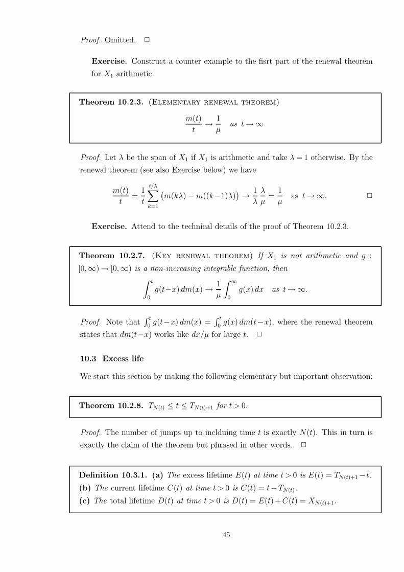
Proof. Omitted. 2
Exercise. Construct a counter example to the fisrt part of the renewal theorem
for X1 arithmetic.
Theorem 10.2.3. (Elementary renewal theorem)
m(t)
t→ 1
µas t→∞.
Proof. Let λ be the span of X1 if X1 is arithmetic and take λ = 1 otherwise. By the
renewal theorem (see also Exercise below) we have
m(t)
t=
1
t
t/λ∑
k=1
(
m(kλ)−m((k−1)λ))
→ 1
λ
λ
µ=
1
µas t→∞. 2
Exercise. Attend to the technical details of the proof of Theorem 10.2.3.
Theorem 10.2.7. (Key renewal theorem) If X1 is not arithmetic and g :
[0,∞)→ [0,∞) is a non-increasing integrable function, then∫ t
0
g(t−x) dm(x)→ 1
µ
∫ ∞
0
g(x) dx as t→∞.
Proof. Note that∫ t
0g(t−x) dm(x) =
∫ t
0g(x) dm(t−x), where the renewal theorem
states that dm(t−x) works like dx/µ for large t. 2
10.3 Excess life
We start this section by making the following elementary but important observation:
Theorem 10.2.8. TN(t) ≤ t ≤ TN(t)+1 for t > 0.
Proof. The number of jumps up to inclduing time t is exactly N(t). This in turn is
exactly the claim of the theorem but phrased in other words. 2
Definition 10.3.1. (a) The excess lifetime E(t) at time t > 0 is E(t) = TN(t)+1−t.
(b) The current lifetime C(t) at time t > 0 is C(t) = t−TN(t).
(c) The total lifetime D(t) at time t > 0 is D(t) = E(t)+C(t) = XN(t)+1.
45
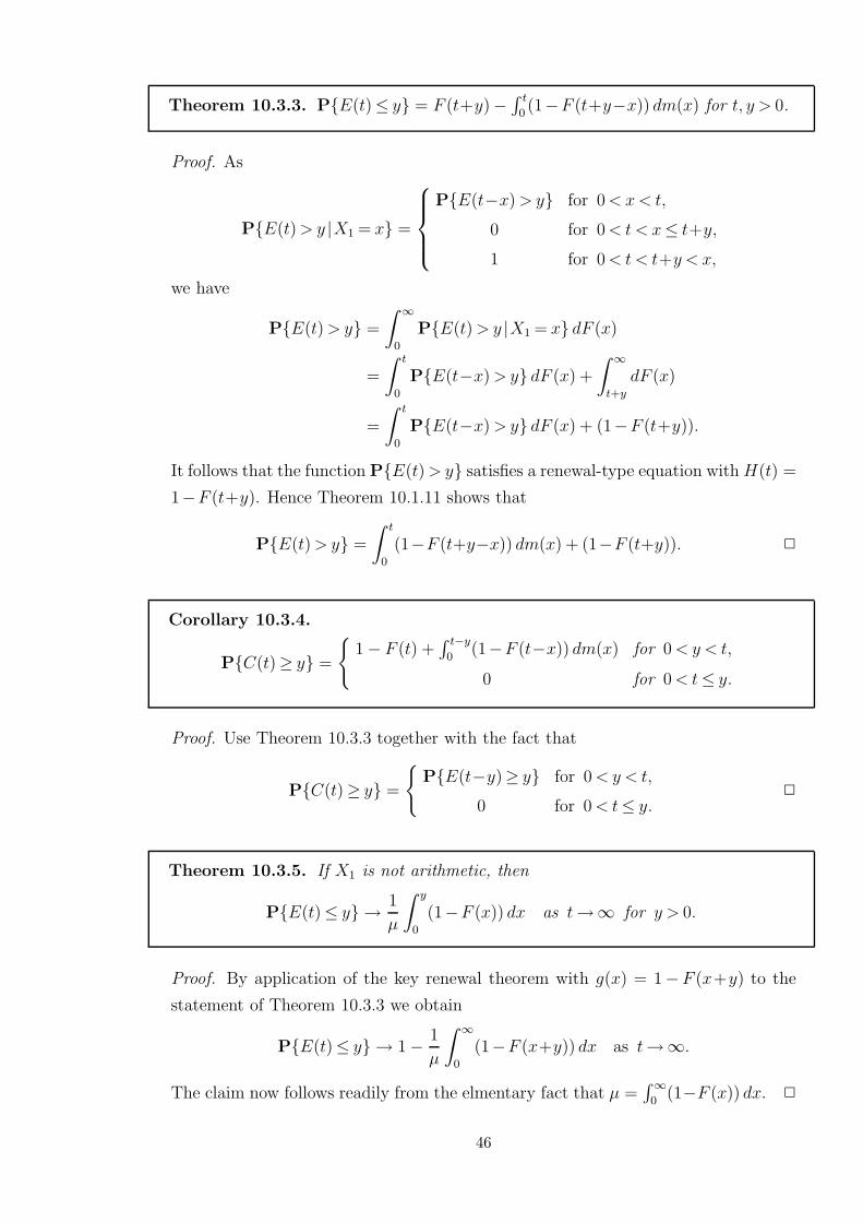
Theorem 10.3.3. PE(t)≤ y = F (t+y)−∫ t
0(1−F (t+y−x)) dm(x) for t, y > 0.
Proof. As
PE(t) > y |X1 = x =
PE(t−x) > y for 0 < x < t,
0 for 0 < t < x≤ t+y,
1 for 0 < t < t+y < x,
we have
PE(t) > y =
∫ ∞
0
PE(t) > y |X1 = x dF (x)
=
∫ t
0
PE(t−x) > y dF (x) +
∫ ∞
t+y
dF (x)
=
∫ t
0
PE(t−x) > y dF (x) + (1−F (t+y)).
It follows that the function PE(t) > y satisfies a renewal-type equation with H(t) =
1−F (t+y). Hence Theorem 10.1.11 shows that
PE(t) > y =
∫ t
0
(1−F (t+y−x)) dm(x) + (1−F (t+y)). 2
Corollary 10.3.4.
PC(t)≥ y =
1− F (t) +∫ t−y
0(1−F (t−x)) dm(x) for 0 < y < t,
0 for 0 < t≤ y.
Proof. Use Theorem 10.3.3 together with the fact that
PC(t)≥ y =
PE(t−y)≥ y for 0 < y < t,
0 for 0 < t≤ y.2
Theorem 10.3.5. If X1 is not arithmetic, then
PE(t)≤ y → 1
µ
∫ y
0
(1−F (x)) dx as t→∞ for y > 0.
Proof. By application of the key renewal theorem with g(x) = 1−F (x+y) to the
statement of Theorem 10.3.3 we obtain
PE(t)≤ y → 1− 1
µ
∫ ∞
0
(1−F (x+y)) dx as t→∞.
The claim now follows readily from the elmentary fact that µ =∫∞
0(1−F (x)) dx. 2
46

Lecture 9, Friday 19 February
10.4 Applications
Example 10.4.1. (Dead periods) Let N(t) be a renewal process with excess
life-time process E(t). Assume that the renewal process is locked a time Li after
the i’th jump of N , so that no new jumps can be made during that locking time.
Here Li∞i=0 are iid. random variables that are independent of N and jumps
during locking times are simply neglected. The process N = N(t)t≥0 that
results from this is started up with an initial locking time L0. Writing Xi∞i=1
for the interarrival times of N Theorem 10.3.3 gives
PX1 ≤ x =
∫ x
0
P
L0+E(L0)≤ x∣
∣L0 = ℓ
dFL(ℓ)
=
∫ x
0
PE(ℓ)≤ x−ℓ dFL(ℓ)
=
∫ x
0
F (ℓ+x−ℓ) dFL(ℓ)−∫ x
0
(∫ ℓ
0
(1−F (ℓ+x−ℓ−z)) dm(z)
)
dFL(ℓ)
= F (x)FL(x)−∫ x
0
m(ℓ)dFL(ℓ) +
∫ x
0
(∫ ℓ∧x
0
F (x−z) dm(z)
)
dFL(ℓ)
= F (x)FL(x)−∫ x
0
m(ℓ)dFL(ℓ) +
∫ x
0
(∫ x
z
F (x−z) dFL(ℓ)
)
dm(z)
= F (x)FL(x)−∫ x
0
m(ℓ)dFL(ℓ) +
∫ x
0
F (x−z) (FL(x)−FL(z)) dm(z).
Here Lemma 10.1.8 shows that∫ x
0F (x−z) dm(z) = m(x)− F (x), so that we get
PX1 ≤ x
= F (x)FL(x)−∫ x
0
m(ℓ)dFL(ℓ) + FL(x) (m(x)−F (x))−∫ x
0
F (x−z)FL(z) dm(z)
=
∫ x
0
FL(ℓ) dm(ℓ)−∫ x
0
F (x−z)FL(z) dm(z)
=
∫ x
0
(1−F (x−z)) FL(ℓ) dm(ℓ).
Now, this is just the distribution of X1, where in general the interarrival times
Xi∞i=1 are neither independent nor identically distributed, so more work is re-
quired to find the distribution of the n’th arrival Tn = X1+ . . . + Xn. However,
when N is a Poisson process the lack of memory property for the exponential
distribution makes N a renewal process with interarrival times Li−1+Xi∞i=1. #
Example 10.4.4. (Alternating renewal process) A machine breaks down
repeatedly, where after the n’th breakdown it is repaired a time Yn after which
it runs a time Zn before its n+1’th breakdown. Here Yn∞n=1 and Zn∞n=0 are
47
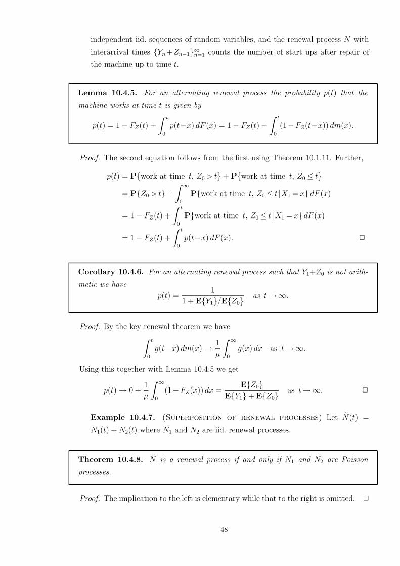
independent iid. sequences of random variables, and the renewal process N with
interarrival times Yn+Zn−1∞n=1 counts the number of start ups after repair of
the machine up to time t.
Lemma 10.4.5. For an alternating renewal process the probability p(t) that the
machine works at time t is given by
p(t) = 1− FZ(t) +
∫ t
0
p(t−x) dF (x) = 1− FZ(t) +
∫ t
0
(1−FZ(t−x)) dm(x).
Proof. The second equation follows from the first using Theorem 10.1.11. Further,
p(t) = Pwork at time t, Z0 > t+ Pwork at time t, Z0 ≤ t
= PZ0 > t+
∫ ∞
0
Pwork at time t, Z0 ≤ t |X1 = x dF (x)
= 1− FZ(t) +
∫ t
0
Pwork at time t, Z0 ≤ t |X1 = x dF (x)
= 1− FZ(t) +
∫ t
0
p(t−x) dF (x). 2
Corollary 10.4.6. For an alternating renewal process such that Y1+Z0 is not arith-
metic we have
p(t) =1
1 + EY1/EZ0as t→∞.
Proof. By the key renewal theorem we have
∫ t
0
g(t−x) dm(x)→ 1
µ
∫ ∞
0
g(x) dx as t→∞.
Using this together with Lemma 10.4.5 we get
p(t)→ 0 +1
µ
∫ ∞
0
(1−FZ(x)) dx =EZ0
EY1+ EZ0as t→∞. 2
Example 10.4.7. (Superposition of renewal processes) Let N(t) =
N1(t) + N2(t) where N1 and N2 are iid. renewal processes.
Theorem 10.4.8. N is a renewal process if and only if N1 and N2 are Poisson
processes.
Proof. The implication to the left is elementary while that to the right is omitted. 2
48

Definition 10.4.12. A (version of a) renewal process Nd = Nd(t)t≥0 where the
first interarrival time X1 has another distribution function F d than the following ones
Xi∞i=2 is called a delayed renewal process.
Theorem. For a delayed renewal process we have
md(t) ≡ ENd(t) = F d(t) +
∫ t
0
m(t−x) dF d(x).
Proof. By analogy with the proof of Lemma 10.1.8 we have
md(t) =
∫ ∞
0
ENd(t) |X1 =x dF d(x)
= 0 +
∫ t
0
EN(t−x)+1 dF d(x)
=
∫ t
0
m(t−x) dF d(x) + F d(t). 2
Theorem 10.4.15. For a delayed renewal process we have
md(t)
t→ 1
µas t→∞.
If X2 is not arithmetic the we further have
md(t+h)−md(t)→ h
µas t→∞ for h≥ 0.
If X2 is arithmetic with span λ then the above limit holds for h a mutiple of λ.
Proof. The time X1 to the first jump of Nd does not affect limit properties of Nd(t)
as t→∞, which are thus the same as those of N . 2
Theorem 10.4.17. A delayed renewal process Nd has stationary increments if and
only if
F d(y) =1
µ
∫ y
0
(1−F (x)) dx for y ≥ 0.
Proof. The implication to the left is omitted. For that to the right we note that if
Nd has stationary increments, then we must have md(t+s) = md(t) + md(s), so that
md(t) = ct for some constant c≥ 0. As a previous theorem gives
md(t) = F d(t) +
∫ t
0
F d(t−x) dm(x),
49

we might use Theorem 10.1.11 to conclude that
F d(t) = md(t)−∫ t
0
md(t−x) dF (x) = md(t)−∫ t
0
F (t−x) dmd(x) = c
∫ t
0
(1−F (x)) dx,
where we get c = 1/µ by sending t→∞. 2
10.5 Renewal-reward processes
Definition. Given a sequence (Xi, Ri)∞i=1 of pairs of iid. random variables such that
PX1 > 0 = 1 and writing Tn =∑n
i=1 Xi, a renewal-reward process C = C(t)t≥0
is given by
C(t) =
N(t)∑
i=1
Ri where N(t) = maxn : Tn ≤ t for t≥ 0.
Definition. The reward function c of a renewal-reward process C is given by c(t) =
EC(t).
Theorem 10.5.1. (Renewal-reward theorem) If EX1 <∞ and E|R1| <
∞, then we have
C(t)
t→ ER1
EX1and
c(t)
t→ ER1
EX1as t→∞.
Proof. By Theorem 10.2.1 together with the strong law of large numbers we have
C(t)
t=
1
t
N(t)∑
i=1
Ri =N(t)
t
1
N(t)
N(t)∑
i=1
Ri →1
EX1ER1 as t→∞.
Since the event that N(t) ≥ i−1 = X1+. . .+Xi−1 ≤ t is independent of Ri the
elementary renewal Theorem 10.2.3 further gives that
c(t)
t=
1
tE
N(t)∑
i=1
Ri
=1
tE
N(t)+1∑
i=1
Ri
− ERN(t)+1t
=1
tE
∞∑
i=1
1N(t)+1≥iRi
− ERN(t)+1t
50
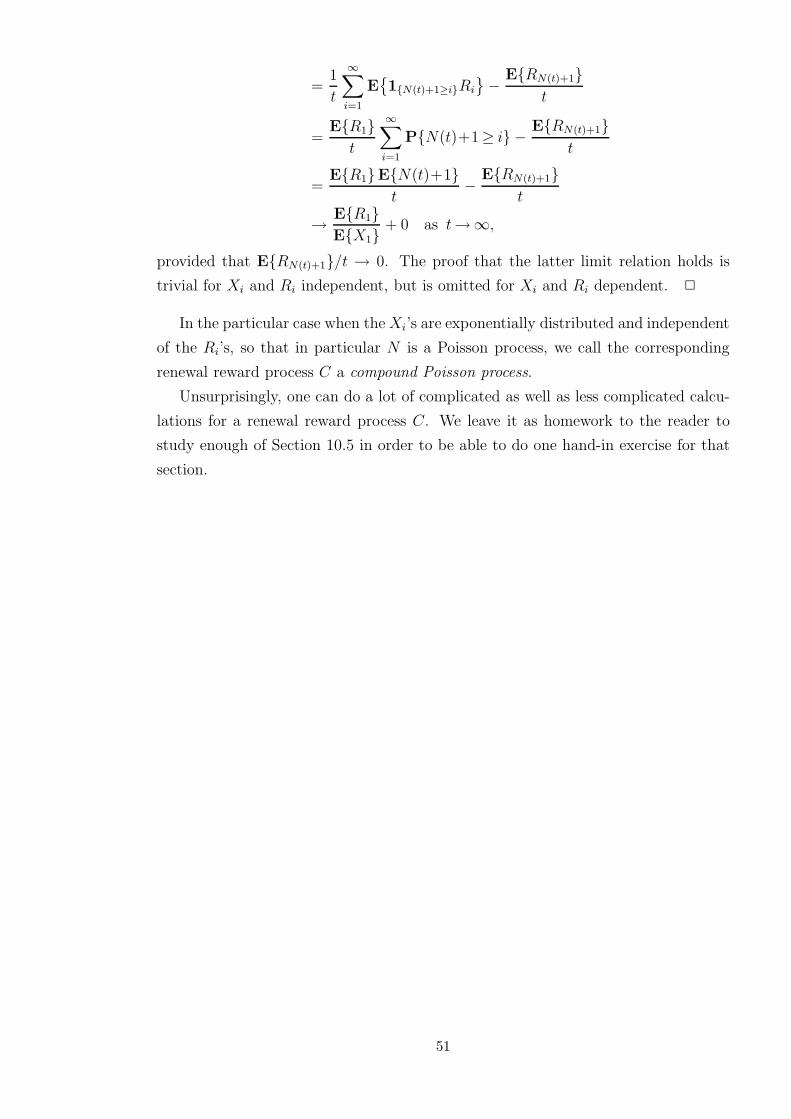
=1
t
∞∑
i=1
E
1N(t)+1≥iRi
− ERN(t)+1t
=ER1
t
∞∑
i=1
PN(t)+1≥ i − ERN(t)+1t
=ER1EN(t)+1
t− ERN(t)+1
t
→ ER1EX1
+ 0 as t→∞,
provided that ERN(t)+1/t → 0. The proof that the latter limit relation holds is
trivial for Xi and Ri independent, but is omitted for Xi and Ri dependent. 2
In the particular case when the Xi’s are exponentially distributed and independent
of the Ri’s, so that in particular N is a Poisson process, we call the corresponding
renewal reward process C a compound Poisson process.
Unsurprisingly, one can do a lot of complicated as well as less complicated calcu-
lations for a renewal reward process C. We leave it as homework to the reader to
study enough of Section 10.5 in order to be able to do one hand-in exercise for that
section.
51

52
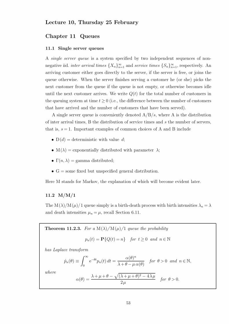
Lecture 10, Thursday 25 February
Chapter 11 Queues
11.1 Single server queues
A single server queue is a system specified by two independent sequences of non-
negative iid. inter arrival times Xn∞n=1 and service times Sn∞n=1, respectively. An
arriving customer either goes directly to the server, if the server is free, or joins the
queue otherwise. When the server finishes serving a customer he (or she) picks the
next customer from the queue if the queue is not empty, or otherwise becomes idle
until the next customer arrives. We write Q(t) for the total number of customers in
the queuing system at time t≥ 0 (i.e., the difference between the number of customers
that have arrived and the number of customers that have been served).
A single server queue is conveniently denoted A/B/s, where A is the distribution
of inter arrival times, B the distribution of service times and s the number of servers,
that is, s = 1. Important examples of common choices of A and B include
• D(d) = deterministic with value d;
• M(λ) = exponentially distributed with parameter λ;
• Γ(n, λ) = gamma distributed;
• G = some fixed but unspecified general distribution.
Here M stands for Markov, the explanation of which will become evident later.
11.2 M/M/1
The M(λ)/M(µ)/1 queue simply is a birth-death process with birth intensities λn = λ
and death intensities µn = µ, recall Section 6.11.
Theorem 11.2.3. For a M(λ)/ M(µ)/1 queue the probability
pn(t) = PQ(t) = n for t≥ 0 and n∈N
has Laplace transform
pn(θ) ≡∫ ∞
0
e−θtpn(t) dt =α(θ)n
λ+ θ−µ α(θ)for θ > 0 and n ∈N,
where
α(θ) =λ+µ+ θ−
√
(λ+µ+ θ)2 − 4λµ
2µfor θ > 0.
53

Proof. Let Pt and G denote the transition matrix and generator, respectively, for the
above mentioned birth-death process. Note that µ(0) is the one-point distribution at
zero, so that Qt = µ(0)Pt = (p0(t) p1(t) . . . ) satisfies Q′t = QtG by the Kolmogorov
forward equations. Spelled out explicitely that system of equations in turn become
p′n(t) = λ pn−1(t)− (λ+µ) pn(t) + µ pn+1(t) for n≥ 1,
p′0(t) = −λ p0(t) + µ p1(t).
Noting that∫ ∞
0
e−θtp′n(t) dt =[
e−θtpn(t)]∞
t=0+ θ
∫ ∞
0
e−θtpn(t) dt = −δ(n) + θ pn(θ),
we may Laplace transform the above system of equations to obtain
λ pn−1(θ)− (λ+µ+ θ) pn(θ) + µ pn+1(θ) = 0 for n≥ 1,
(λ+ θ) p0(θ)− µ p1(θ) = 1.
From difference equation techniques it is known that the first of these equations has
two solutions, namely
pn(θ) =
(
λ+µ+ θ−√
(λ+µ+ θ)2 − 4λµ
2µ
)n
p0(θ) = α(θ)n p0(θ) for n≥ 1
and
pn(θ) =
(
λ+µ+ θ +√
(λ+µ+ θ)2 − 4λµ
2µ
)n
p0(θ) for n≥ 1.
Here the second solution must be invalid as the value of pn(θ) because pn(θ) ≤ 1/θ
for n ≥ 0, while the second solution goes to ∞ as n → ∞ for θ > 0 sufficiently
large. (As p0 is an analytic function it can not be zero for large θ.) Now we may
insert p1(θ) = α(θ) p0(θ) in the equation (λ+θ) p0(θ)− µ p1(θ) = 1 to obtain p0(θ) =
1/(λ+ θ−µ α(θ)). This proves the claim of the theorem. 2
Definition. The traffic intensity ρ of a queue is given by ρ = ES/EX.
Unsurprisingly the qualitative behaviour of an M(λ)/M(µ)/1 queue depends on
whether ρ < 1 or ρ≥ 1:
Theorem 11.2.8. Consider a M(λ)/ M(µ)/1 queue with traffic intensity ρ = λ/µ.
(a) If ρ < 1 then PQ(t) = n → πn as t→∞ where πn = (1− ρ) ρn is the unique
stationary distribution.
(b) If ρ ≥ 1 then PQ(t) = n → 0 as t → ∞ and there exists no stationary
distribution.
54

Proof. This follows from the limit Theorem 6.9.21 for continuous time Markov chains
together with the second last example of Section 6.11. 2
Let Un∞n=1 be the sequence of times at which the number of customers Q(t) in
a M(λ)/M(µ)/1 queue changes. Setting Qn = Q(U+n ) for n ≥ 1 and Q0 = 0 we see
that Qn∞n=0 is a discrete time Markov chain such that
Qn+1 =
Qn +1 with probabilityλ
λ+µ=
ρ
1+ρ
Qn−1 with probabilityµ
λ+µ=
1
1+ρ
for Qn ≥ 1,
while Qn+1 = 1 for Qn = 0. In other words, Qn∞n=0 is a random walk on the
non-negative integers with a reflecting barrier at zero.
Looking for a stationary distribution for the Markov chain Qn∞n=0 we study the
system of equations π P = π, which spelled out becomes
1
1+ρπ1 = π0,
π0 +1
1+ρπ2 = π1,
ρ
1+ρπn−1 +
1
1+ρπn+1 = πn for n≥ 2.
From difference equation techniques it is known that the last of these equations has
two solutions, namely
πn = π1 for n≥ 2 and πn = ρn−1 π1 for n≥ 2.
In order for π to be a stationary distribution we must disregard the first of these
solution, while the second solution will give a stationary distribution if and only if
ρ < 1. In the latter case we may insert π2 = ρ π1 in the first two equations of the
system of equations π P = π to see that they reduce to π1 = (1+ρ) π0. Using that∞∑
n=0
πn = π0 + (1+ρ) π0 +
∞∑
n=2
(1+ρ) ρn−1π0 = . . . =2
1−ρπ0,
we conclude that the chain is non-null persistent with stationary distribution
π0 =1−ρ
2and πn =
1−ρ2
2ρn−1 for n≥ 1
when ρ < 1. Unsurprisingly, it can be shown that the chain is null persistent for
ρ = 1, while it is transistent for ρ > 1. We leave this as an exercise to the reader.
Exercise. (Difficult) Prove that the Markov chain Qn∞n=0 is null persistent
when ρ = 1 and transistent for ρ > 1.
The chain Qn∞n=0 is called an imbedded Markov chain, and we shall see in the
following two sections that such imbedding techniques are important for the study of
M/G/1 and G/M/1 queues.
55

11.3 M/G/1
Let Dn be the time at which the n’th customer departs from a M(λ)/G/1 queue for
n≥ 1. Set Qn = Q(D+n ) for n≥ 1 and Q0 = 0.
Theorem 11.3.4. For a M(λ)/G/1 queue the sequence Qn∞n=0 is a discrete time
Markov chain with transition matrix
P =
δ0 δ1 δ2 δ3 δ4 · · ·δ0 δ1 δ2 δ3 δ4 · · ·0 δ0 δ1 δ2 δ3 · · ·0 0 δ0 δ1 δ2 · · ·0 0 0 δ0 δ1 · · ·...
......
......
. . .
,
where δ is the probability distribution on N with entries
δj = E
(λS)j
j!e−λS
for j ∈N.
Proof. Writing An for the number of customers that arrive during the service time
of the n’th customer, we have
Qn+1 = Q(D+n+1) =
An+1 +Q(D+n )−1 if Qn > 0,
An+1 if Qn = 0.
It follows that
PQn+1 = j |Qn = i =
PAn+1 = j−i+1 for j ≥ i > 0,
PAn+1 = j for j ≥ i = 0.
As each An is Po(λS) distributed the claim of the theorem follows. 2
Theorem 11.3.5. Consider a M(λ)/G/1 queue with traffic intensity ρ = λES.(a) If ρ < 1 then the chain Qn∞n=0 is ergodic with a unique stationary distribution
π having generating function
Gπ(s) =
∞∑
j=0
sj πj = (1−ρ) (s−1)MS(λ (s−1))
s−MS(λ (s−1))for s ∈ [0, 1),
where MS(t) = EetS is the moment generating function of S.
(b) If ρ = 1 then the chain Qn∞n=0 is null persistent.
(c) If ρ > 1 then the chain Qn∞n=0 is transient.
56

Proof. We omit the proof of claims b and c, but note that they are very natural and
expected. As for the proof of claim a, we note that Theorem 11.3.4 shows that the
equation π = π P takes the form
πj = π0δj +
j+1∑
i=1
πi δj−i+1 for j ∈N.
Writing ∆(s) =∑∞
j=0 sj δj for the generating function of δ it follows that
Gπ(s) =
∞∑
j=0
sj πj
= π0 ∆(s) +∞∑
j=0
sj
(
j+1∑
i=1
πi δj−i+1
)
= π0 ∆(s) +∞∑
i=1
πi si−1
(
∞∑
j=i−1
sj−(i−1) δj−(i−1)
)
= π0 ∆(s) +Gπ(s)−π0
s∆(s),
so that by rearrangement
Gπ(s) =∆(s) (s−1)
s−∆(s)π0.
Here we may use the Taylor expansion
∆(s) = ∆(1) + (s−1) ∆′(1) + o(s−1) = 1 + (s−1) ∆′(1) + o(s−1) as s ↑ 1
to conclude that
1← Gπ(s) =∆(s) (s−1)
s−∆(s)π0 →
1
1−∆′(1)π0 as s ↑ 1,
so that
Gπ(s) =∆(s) (s−1)
s−∆(s)(1−∆′(1)).
Now it is sufficient to check that ∆(s) = MS(λ (s−1)) = EeλS(s−1), because then
∆′(1) = EλS = ρ, and the claim of the theorem follows. However,
∆(s) =
∞∑
j=0
sj E
(λS)j
j!e−λS
= E
eλsSe−λS
= MS(λ (s−1)). 2
Corollary 11.3.6. A busy period B during which the server is continuously occupied
for a M(λ)/G/1 queue satisfies
(a) EB <∞ for ρ < 1;
(b) EB =∞ and PB <∞ = 1 for ρ = 1;
(c) PB <∞ < 1 for ρ > 1.
57

Proof. As B is the reccurence time for the state 0 for the chain Qn∞n=0, the corollary
follows immediately from Theorem 11.3.5. 2
Theorem 11.3.16. The waiting time W a customer has to wait in the queue after
arrival before coming to the server for a M(λ)/G/1 queue with traffic intensity ρ < 1
in equilibrium has moment generating function
MW (s) =(1−ρ) s
λ+ s− λ MS(s).
Proof. Equilibrium means that the queue follows its stationary distribution, which is
to say that it is started according to that distribution. Then with obvious notation a
customer that waits a time W leaves a Po(λ(W+S)) distributed number of customers
behind him (or her) in the queue. Using this together with Theorem 11.3.5 we get
(1−ρ) (s−1)MS(λ (s−1))
s−MS(λ (s−1))= E
sQn+1
= E
sPo(λ(W+S))
=∞∑
k=0
sk E
(λ(W +S))k
k!e−λ(W+S)
= E
eλ(s−1)(W+S)
= MW (λ(s−1)) MS(λ(s−1)),
so that
MW (λ(s−1)) =(1−ρ) λ (s−1)
λ + λ (s−1)− λ MS(λ (s−1)). 2
Theorem 11.3.17. The moment generating function MB for the busy period B of
a M(λ)/G/1 queue with traffic intensity ρ < 1 in equilibrium satisfies the equation
MB(s) = MS
(
s−λ+λ MB(s))
.
Proof. Defining A as in the proof of Theorem 11.3.4 we have with obvious notation
that B = S +∑A
j=1 Bj. Recalling that A is Po(λS) distributed we may condition on
the value of S to obtain
MB(s) = E
es(S+PA
j=1Bj)
=
∫ ∞
0
∞∑
k=0
E
es(x+Pk
j=1Bj) (λx)k
k!e−λx dFS(x)
=
∫ ∞
0
esx+(MB(s)−1)λx dFS(x)
= MS
(
s−λ+λ MB(s))
. 2
58

Lecture 11, Friday 26 February
11.4 G/M/1
Let Tn be the time at which the n’th customer arrives to the queuing system for a
G/ M(µ)/1 queue for n≥ 1. Set Qn = Q(T−n+1) for n≥ 0.
Theorem 11.4.3. For a G/ M(µ)/1 queue the sequence Qn∞n=0 is a discrete time
Markov chain with transition matrix
P =
1−α0 α0 0 0 0 · · ·1−α0−α1 α1 α0 0 0 · · ·
1−α0−α1−α2 α2 α1 α0 0 · · ·1−α0−α1−α2−α3 α3 α2 α1 α0 · · ·
1−α0−α1−α2−α3−α4 α4 α3 α2 α1 · · ·...
......
......
. . .
,
where α is the probability distribution on N with entries
αj = E
(µX)j
j!e−µX
for j ∈N.
Proof. If Vn is the number of customers that depart from the queuing system during
the time interval [Tn, Tn+1), then we have Qn+1 = Qn +1−Vn for n≥ 0. Here Vn has
a truncated Po(µXn+1) distribution, which is to say
PQn+1 = j |Qn = i = PVn = i+1−j =
E
(µX)i+1−j
(i+1−j)!e−µX
if 1≤ j ≤ i+1,
∑
k>i
E
(µX)k
k!e−µX
if j = 0.2
Theorem 11.4.4. Consider a G/ M(µ)/1 queue with traffic intensity ρ = 1/(µEX).(a) If ρ < 1 then the chain Qn∞n=0 is ergodic with a unique stationary distribution π
given by πj = (1−η) ηj for j ∈N, where η is the smallest positive root to the equation
η = MX(µ (η−1)) and MX is the moment generating function for X.
(b) If ρ = 1 then the chain Qn∞n=0 is null persistent.
(c) If ρ > 1 then the chain Qn∞n=0 is transient.
Proof. Taking off from Theorem 11.4.3, the proof of this theorem is very similar
to that of Theorem 11.3.5 (taking off from Theorem 11.3.4). The proof is therefore
omitted. 2
59

Theorem 11.4.12. The waiting time W a customer has to wait in the queue after
arrival before coming to the server for a G/ M(µ)/1 queue with traffic intensity ρ < 1
in equilibrium has distribution function
PW ≤ x =
0 if x < 0,
1− η if x = 0,
1− η e−µ(1−η)x if x > 0,
where η is as in Theorem 11.4.4.
Proof. By the lack of memory property the waiting time Wn for the n’th customer
that arrives to the queue is the sum of Qn−1 independent exponentially distributed
random variables with parameter µ. Using this together with Theorem 11.4.4 we get
MW (s) =
∞∑
j=0
(Eexp(µ))jπj =
∞∑
j=0
(
µ
µ− s
)j
(1−η) ηj = · · · = (1−η)+ηµ(1−η)
µ(1−η)− s,
which is to say a mixture of a distribution that is zero with probability 1−η and an
exponential distribution with parameter µ(1−η) with probability η. 2
11.5 G/G/1
Theorem 11.5.1. (Lindley’s14 equation) For a G/G/1 queue we have
Wn+1 = max
0, Wn +Sn−Xn+1
.
Proof. Writing Tn for the arrival time of the n’th customer to the queuing system
and noting that Tn+1−Tn = Xn+1 we readily see that
Tn+1 + Wn+1 = max
Tn+1, Tn + Wn + Sn
.
Subtracting Tn+1 from both sides of this equation we get the claim of the theorem. 2
Theorem 11.5.2. For a G/G/1 queue we have
PWn+1 ≤ x =
0 if x < 0,∫ x
−∞
PWn≤ x−y dG(y) if x≥ 0,
where G is the distribution function of Un = Sn−Xn+1. In particular it follows that
the limit limn→∞ PWn≤ x exists.
14Dennis Victor Lindley, British statistician born 1923.
60

Proof. The first claim follows from Lindley’s equation. As for the second claim, it
is sufficient to prove that PWn+1 ≤ x ≤ PWn ≤ x for all n and x. Now this is
trivially true for n = 1 as PW1 ≤ 0 = 1. Further, if the inequality holds for all x
for n = k, then it holds for all x for n = k+1 by the first claim of the theorem. 2
Theorem 11.5.7. For a G/G/1 queue the random variable Wn+1 has the same
distribution as
W ′n+1 ≡ max
0, U1, U1+U2, . . . , U1+. . .+Un
.
Proof. Use Lindley’s equation to deduce that W1 = 0, W2 = max0, W1 +U1 =
max0, U1, W3 = max0, W2+U2 = max0, U2, U1+U1, . . . , Wn+1 = max0, Un,
Un+Un−1, . . . , Un+. . .+U1. Then use that the vectors (U1, . . . , Un) and (Un, . . . , U1)
are identically distributed. 2
Theorem 11.5.4. Consider a G/G/1 queue with traffic intensity ρ = ES/EX.(a) If ρ < 1 then the limit F (x) = limn→∞ PWn≤ x is a distribution function.
(b) If ρ = 1 and VarU > 0 then F (x) = 0 for x∈R.
(c) If ρ > 1 then F (x) = 0 for x ∈R.
Proof. We omit the proof of claims b and c, but note that they are very natural
and expected. As for claim a we note that W ′n ≤ W ′
n+1 for all n, so that the limit
limn→∞ W ′n = W ′ exists. Using Theorem 11.5.7 we now get
F (x) = limn→∞
PW ′n≤ x = PW ′ ≤ x = P
∑n
j=1 Uj ≤ x for all n
.
As we assume ρ < 1, which is to say EU < 0, the strong law of large numbers gives
P∑n
j=1 Uj > 0 for infinitely many n
= P
1
n
n∑
j=1
Uj −EU > −EU for infinitely many n
= 0.
Hence W ′ is with probability 1 the maximum of only finitely many members of the
sequence ∑n
j=1 Uj∞n=1, and thus a well-defined finite random variable. 2
11.6 Heavy traffic
Many real-world queues are designed to have a traffic intensity ρ strictly less than one
(for reasons of stability), but just barely so (for reasons of economy). It is therefore
interesting to investigate the behaviour of a queue as ρ ↑ 1. The following theorem
exemplifies such an investigation:
61

Theorem 11.6.1. Let a M(λ)/D(d)/1 queue have traffic intensity ρ = dλ < 1.
If Qρ is a random variable with the stationary distribution (recall Theorem 11.3.5),
then (1−ρ) Qρ converges in distribution to an exponential distribution with expected
value 1/2 as ρ ↑ 1.
Proof. As MS(t) = etd Theorem 11.3.5 shows that
M(1−ρ)Qρ(s) = MQρ((1−ρ) s)
= Gπ
(
e(1−ρ)s)
= (1−ρ) (e(1−ρ)s−1)exp
ρ (e(1−ρ)s−1)
e(1−ρ)s− exp
ρ (e(1−ρ)s−1)
=(1−ρ) (e(1−ρ)s−1)
exp
(1−ρ) s−ρ (e(1−ρ)s−1)
− 1
=(1−ρ)
(
(1−ρ) s+ o(1−ρ))
(1−ρ)2s− (1−ρ)2s2/2+ o((1−ρ)2)
→ 2
2− s
=
∫ ∞
0
esx 2 e−2x dx as ρ ↑ 1. 2
62

Lecture 12, Thursday 4 March
Chapter 12 Martingales
In this chapter we will be much concerned with conditional expectations and proba-
bilities. Given random variables X0, . . . , Xn, Y , recall that
EY |X0 =x0, . . . , Xn =xn = f(x0, . . . , xn)
and
PY ≤y |X0 =x0, . . . , Xn =xn = g(y, x0, . . . , xn)
are functions of x0, . . . , xn and y, x0, . . . , xn, respectively. Hence we may define
EY |X0, . . . , Xn = f(X0, . . . , Xn)
and
PY ≤y |X0, . . . , Xn = g(y, X0, . . . , Xn),
so that EY |X0, . . . , Xn and PY ≤y |X0, . . . , Xn become random variables.
12.1 Introduction
Definition 12.1.1. A sequence Yn∞n=0 of random variables is a martingale15 with
respect to a sequence Xn∞n=0 of random variables if
E|Yn| <∞ and EYn+1|X0, . . . , Xn = Yn for all n.
The most common selection of the sequence Xn∞n=0 is to take it to be equal to
Yn∞n=0, so that the martingale definition boils down to
E|Yn| <∞ and EYn+1|Y0, . . . , Yn = Yn for all n.
Whatever the choice of the sequence Xn∞n=0 we write Fn to denote the information
corresponding to the knowledge of the random variables Xn∞n=0, so that
EY |X0, . . . , Xn = EY |Fn.
Two important formulae associated with this formalism is that
E
EY |Fm+n∣
∣Fn
= EY |Fn and E
EY |Fn∣
∣Fm+n
= EY |Fn
for m+n≥ n≥ 0.
15See http://www.emis.de/journals/JEHPS/juin2009/Mansuy.pdf for information on the origin of the
word martingale. (It is not a person!)
63

Example 12.1.2. (Simple random walk) Let Yn =∑n
i=1 Xi−n (p−q) where
Xn∞n=0 are iid. −1, 1-valued random variables such that PXn = 1 = p and
PXn = −1 = q = 1− p. Then it is clear that Yn∞n=0 is a martingale with
respect to Xn∞n=0, see exercise below. #
Exercise. Prove the claim of Example 12.1.2 in full detail.
Example 12.1.4. (De Moivre’s16 martingale) Take Xn∞n=0 as in Examp-
le 12.1.2 and define Yn = (q/p)X1+...+Xn . Then Yn∞n=0 is a martingale with
respect to Xn∞n=0 because
EYn+1|X0, . . . , Xn = (q/p)X1+...+Xn E
(q/p)Xn+1
= Yn
(q
pp +
p
qq)
= Yn. #
Definition 12.1.9. (a) A sequence Yn∞n=0 of random variables is a submartingale
with respect to Fn∞n=0 if
E|Yn| <∞17, EYn|Fn = Yn and EYn+1|Fn ≥ Yn for all n.
(b) A sequence Yn∞n=0 of random variables is a supermartingale with respect to
Fn∞n=0 if
E|Yn| <∞, EYn|Fn = Yn and EYn+1|Fn ≤ Yn for all n.
Clearly, a process that is both a submartingale and a supermartingale (with re-
spect to a common sequence) is a martingale (with respect to that sequence). Also,
if Yn∞n=0 is a submartingale then −Yn∞n=0 is a supermartingale, and vice versa.
Proposition. A submartingale have non-decreasing mean.
Proof. We have
EYn+1 = EEYn+1|Fn ≥ EYn. 2
By the above proposition together with the text following Definition 12.1.9 mar-
tingales have constant means while supermartingales have non-increasing means.
The next theorem is quit basic and follows from a few simple arguments, but is
of fundamental importance anyway:
16Abraham de Moivre, French mathematician 1667-1754.
17The weaker integrability condition employed by Grimmett and Stirzaker in their definition of submartin-
gales and supermartingales is wrong!
64

Theorem. (a) If Yn∞n=0 is a martingale and g : R→R a convex function such that
E|g(Yn)| <∞ for all n, then g(Yn)∞n=0 is a submartingale.
(b) If Yn∞n=0 is a submartingale and g : R→ R a non-decreasing convex function
such that E|g(Yn)| <∞ for all n, then g(Yn)∞n=0 is a submartingale.
Proof. This is Exercises 12.1.6 and 12.1.7, respectively, in the book. 2
The next theorem turns out to be one of the few most important results for the
build up of the more advanced martingale theory:
Theorem 12.1.10. (Doob18 decomposition) A submartingale Yn∞n=0 with re-
spect to Fn∞n=0 may be expressed in a unique way as Yn = Mn + Sn where Mn∞n=0
is a martingale with respect to Fn∞n=0 and Sn∞n=0 is a non-decreasing process with
S0 = 0 such that ESn+1|Fn = Sn+1 for all n.
Proof. As for uniqueness we note that if we have two representations Yn = Mn +Sn
and Yn = M ′n +S ′
n for Y of the stipulated type, then
S ′n+1−S ′
n = ES ′n+1−S ′
n|Fn = EYn+1−Yn|Fn = ESn+1−Sn|Fn = Sn+1−Sn.
From this together with a telescope sum argument and the fact that S0 = S ′0 = 0 we
get Sn = S ′n, which in turn gives Mn = M ′
n.
As for existence, define M and S recursively by M0 = Y0, S0 = 0,
Mn+1 = Mn + Yn+1−EYn+1|Fn and Sn+1 = Sn−Yn +EYn+1|Fn for n≥ 1.
By adding the last two equations we see that Mn+1−Mn+ Sn+1−Sn = Yn+1−Yn for
n ≥ 1, so that a telescope sum argument together with the fact that M0 + S0 = Y0
give Yn = Mn +Sn. Further, EMn+1|Fn = Mn holds for n = 0, since
EM1|F0 = EM0|F0 = EY0|F0 = Y0 = M0.
If EMn+1|Fn = Mn holds for n = k then we further have
EMk+2|Fk+1 = E
Mk+1+Yk+2−EYk+2|Fk+1∣
∣Fk+1
= EMk+1|Fk+1= E
Mk+Yk+1−EYk+1|Fk∣
∣Fk+1
= EMk|Fk+1+ Yk+1− EYk+1|Fk= Mk + Yk+1− EYk+1|Fk= Mk+1,
18Joseph Leo Doob, American mathematician 1910-2004, who made founding contributions to the theory
of stoachastic processes and in particular to martingale theory.
65

because
EMk|Fk+1 = E
EMk+1|Fk∣
∣Fk+1
= EMk+1|Fk = Mk.
As it is obvious that the S process is non-decreasing (when Y is a submartingale),
it remains to prove that ESn+1|Fn = Sn+1, which in turn by inspection of the
definition of S holds if ESn|Fn = Sn. As the latter equation holds if ESn|Fn−1= Sn (see exercise below), it is sufficient to prove that ES1|F0 = S1, which in turn
holds by inspection of the definition of S. 2
Exercise. Show that ESn|Fn = Sn if ESn|Fn−1 = Sn in the proof of The-
orem 12.1.10.
12.2 Martingale differences (but not Hoeffding’s inequality)
Definition 12.2.1. A sequence Dn∞n=1 of random variables are martingale differ-
ences if
E|Dn| <∞, EDn|Fn = Dn and EDn+1|Fn = 0 for all n.
Theorem. Dn∞n=1 are martingale differences if and only if ∑n
i=1 Di∞n=0 is a
martingale.
Exercise. Prove the above theorem.
12.3 Crossings and convergence
Historically, martingale theory emerged from a desire to generalize the classical limit
theorems in probability from iid. sequences of random variables to more general set-
tings. The following theorem is just one example of a limit theorem for martingales:
Theorem 12.3.1. If Yn∞n=0 is a submartingale such that supn≥0 E|Yn| < ∞,
then Yn→ Y∞ as n→∞ for some random variable Y∞.
Proof. Omitted. 2
Theorem 12.3.7. If Yn∞n=0 is either a non-positive submartingale or a non-
negative supermartingale, then Yn→ Y∞ as n→∞ for some random variable Y∞.
66

Proof. The first statement follows from Theorem 12.3.7 together with the fact that
submartingales have non-decreasing expectations, so that
supn≥0
E|Yn| = supn≥0
E−Yn = − infn≥0
EYn = −EY0 <∞.
The second statement follows from applying the first statement to −Yn∞n=0. 2
Example 12.3.9. (Doob’s martingale) Let Z be an integrable random vari-
able E|Z| <∞ and set Yn = EZ |Fn for n ∈N. Then we have
E|Yn| = E∣
∣EZ |Fn∣
∣
≤ E
E|Z| |Fn∣
∣
= E|Z| <∞ for n∈N,
as well as
EYn+1|Fn = E
EZ |Fn+1∣
∣Fn = EZ |Fn = Yn for n∈N.
Hence Yn∞n=0 is a martingale that statisfies the hypothesis of Theorem 12.3.7,
so that Yn→ Y∞ as n→∞ for some random variable Y∞. #
12.4 Stopping times
Definition 12.4.1. An N-valued random variable T is called a stopping time (or
optional time) if
PT = n |Fn = 1T=n for n∈N.
Exercise. Show that if T is a stopping time, then we have
PT ≤m |Fn = 1T≤m for m≤ n and PT > n |Fn = 1T>n.
Example 12.4.3. (Coin tossing) Let Xn = 1 if the n’th throw of a fair coin
gives a head while Xn = 0 if the n’th throw gives tails. Then the first time T for
a head is a stopping time with respect to Xn∞n=0, because
PT = n |X0, . . . , Xn = 1X0=...=Xn−1=0,Xn=1 = 1T=n. #
Example 12.4.4. (First passage time) The argument employed in Example
12.4.3 extends to show that T = infn ∈ N : Xn ∈ B is a stopping time with
respect to a given sequence of random variables Xn∞n=0 for any set B ⊆R. #
Theorem 12.4.5. If Yn∞n=0 is a submartingale and T a stopping time, then
Yn∧T∞n=0 is a submartingale.
67

Proof. We have
Yn∧T =
n∑
k=0
Yk 1T=k + Yn 1T>n
From this it follows that
E|Yn∧T | ≤n∑
k=0
E|Yk|+ E|Yn| <∞
as well as (by inspection) EYn∧T |Fn = Yn∧T . Further, we have
EY(n+1)∧T |Fn = E
n+1∑
k=0
Yk 1T=k + Yn+1 1T>n+1
∣
∣
∣
∣
∣
Fn
= E
Yn∧T + Yn+1 1T=n+1 − Yn 1T>n + Yn+11T>n+1
∣
∣
∣
∣
∣
Fn
= Yn∧T + E
(Yn+1−Yn) 1T>n
∣
∣Fn
= Yn∧T + EYn+1−Yn|Fn 1T>n
= Yn∧T +(
EYn+1|Fn − Yn
)
1T>n
≥ Yn∧T
as Y is a submartingale. 2
Theorem 12.4.7. (Optional switching) If Xn∞n=0 and Yn∞n=0 are martin-
gales and T a stopping such that XT = YT , then the following process Zn∞n=0 is a
martingale:
Zn =
Xn for T ≤ n,
Yn for T > n,for n∈N.
Proof. By the martingale properties of X and Y and the fact that XT = YT we have
Zn = EXn+1|Fn 1T≤n + EYn+1|Fn 1T>n
= E
Xn+1 1T≤n + Yn+11T>n
∣
∣Fn
= E
Zn+1 −Xn+1 1T=n+1 + Yn+11T=n+1
∣
∣Fn
= EZn+1|Fn − E
(XT−YT ) 1T=n+1
∣
∣Fn
= EZn+1|Fn. 2
Theorem 12.4.11. (Optional sampling theorem) For a submartingale Yn∞n=0
and a stopping time T that is bounded above by a deterministic finite constant we have
E|YT | <∞ and EYT |F0 ≥ Y0.
68

Proof. By Theorem 12.4.5 Zn = Yn∧T , n∈N, is a submartingale. Selecting an N ∈N
such that T ≤N it follows that E|YT | <∞ in the same way as the first part of the
proof of Theorem 12.4.5. Further, we have
EYT |F0 = EZN |F0 ≥ Z0 = Y0. 2
Theorem 12.4.13. For a martingale Yn∞n=0 we have
P
max0≤k≤n
Yk ≥ x
≤ EY +n
xand P
max0≤k≤n
|Yk| ≥ x
≤ E|Yn|x
for x > 0.
Proof. The second inequality follows from the first one as
P
max0≤k≤n
|Yk| ≥ x
≤ P
max0≤k≤n
Yk ≥ x
+ P
max0≤k≤n
−Yk ≥ x
≤ EY +n
x+
EY −n
x
=E|Yn|
x.
As for the first inequality, write T = infn ∈ N : Yn ≥ x. Then Example 12.4.4
shows that T is a stopping time with respect to Yn∞n=0, from which it follows that
T is also a stopping time with respect to Fn∞n=0, see the exercise below. Hence
T ∧n is a bounded stopping time (see the exercise below), so that
EYT∧n = E
EYT∧n|F0
= EY0 = EYn
by the optional sampling theorem together with the martingale property of Y . It
follows that
EY +n ≥ EY +
n 1T≤n≥ EYn 1T≤n= EYn −EYn 1T>n= EYT∧n −EYT∧n 1T>n= EYT∧n1T≤n= EYT 1T≤n≥ xE1T≤n= xPT ≤ n. 2
Exercise. In the proof of Theorem 12.4.13, show that T is a stopping time with
respect to Fn∞n=0 when it is a stopping time with respect to Yn∞n=0, and that
T ∧n is a stopping time when T is a stopping time.
69

70
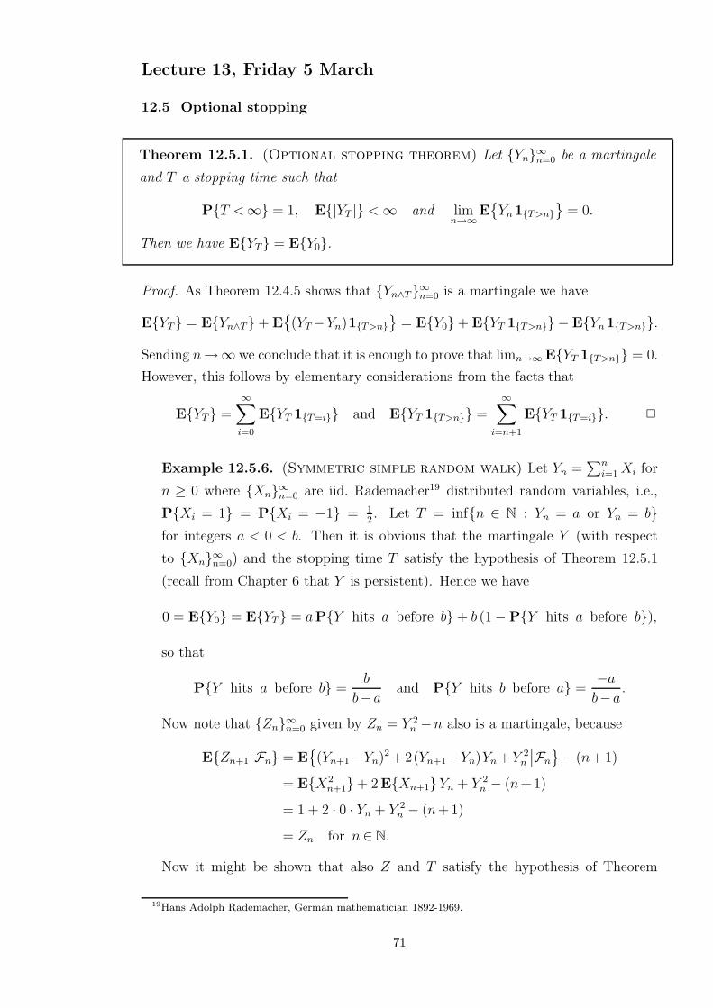
Lecture 13, Friday 5 March
12.5 Optional stopping
Theorem 12.5.1. (Optional stopping theorem) Let Yn∞n=0 be a martingale
and T a stopping time such that
PT <∞ = 1, E|YT | <∞ and limn→∞
E
Yn 1T>n
= 0.
Then we have EYT = EY0.
Proof. As Theorem 12.4.5 shows that Yn∧T∞n=0 is a martingale we have
EYT = EYn∧T+ E
(YT−Yn)1T>n
= EY0+ EYT 1T>n −EYn 1T>n.
Sending n→∞ we conclude that it is enough to prove that limn→∞ EYT 1T>n = 0.
However, this follows by elementary considerations from the facts that
EYT =∞∑
i=0
EYT 1T=i and EYT 1T>n =∞∑
i=n+1
EYT 1T=i. 2
Example 12.5.6. (Symmetric simple random walk) Let Yn =∑n
i=1 Xi for
n ≥ 0 where Xn∞n=0 are iid. Rademacher19 distributed random variables, i.e.,
PXi = 1 = PXi = −1 = 12. Let T = infn ∈ N : Yn = a or Yn = b
for integers a < 0 < b. Then it is obvious that the martingale Y (with respect
to Xn∞n=0) and the stopping time T satisfy the hypothesis of Theorem 12.5.1
(recall from Chapter 6 that Y is persistent). Hence we have
0 = EY0 = EYT = aPY hits a before b + b (1−PY hits a before b),
so that
PY hits a before b =b
b−aand PY hits b before a =
−a
b−a.
Now note that Zn∞n=0 given by Zn = Y 2n −n also is a martingale, because
EZn+1|Fn = E
(Yn+1−Yn)2 +2(Yn+1−Yn)Yn +Y 2n
∣
∣Fn
− (n+1)
= EX2n+1+ 2EXn+1 Yn + Y 2
n − (n+1)
= 1 + 2 · 0 · Yn + Y 2n − (n+1)
= Zn for n∈N.
Now it might be shown that also Z and T satisfy the hypothesis of Theorem
19Hans Adolph Rademacher, German mathematician 1892-1969.
71

12.5.1, see exercise below. Hence we have
0 = EZ0 = EZT = a2 b
b−a+ b2 −a
b−a−ET,
so that we get ET = −ab by rearranging. #
Exercise. Explain in detail why the process Y and the stopping time T in Ex-
ample 12.5.6 satisfy the hypothesis of Theorem 12.5.1.
Exercise. (Difficult) Explain in detail why the process Z and the stopping
time T in Example 12.5.6 satisfy the hypothesis of Theorem 12.5.1.
Example 12.5.12. (Wald’s20 equation) Let Xn∞n=0 be iid. integrable ran-
dom variables and T a stopping time with finite mean. Then we have
E
T∑
n=1
Xn
= EX1ET.
This can be proved by application of Theorem 12.5.1. However, as it is not easy to
verify the hypothesis of that theorem for the setting under consideration it turns
out to be more convenient to prove the result by direct calculations as follows:
E
T∑
n=1
Xn
−EX1ET = E
T∑
n=1
(Xn−EX1)
= E
∞∑
i=1
i∑
n=1
(Xn−EX1) 1T=i
= E
∞∑
n=1
∞∑
i=n
(Xn−EX1) 1T=i
=∞∑
n=1
E
(Xn−EX1) 1T≥n
= −∞∑
n=1
E
(Xn−EX1) 1T≤n−1
= −∞∑
n=1
E
E
(Xn−EX1) 1T≤n−1
∣
∣Fn−1
= −∞∑
n=1
E
E
(Xn−EX1)∣
∣Fn−1
1T≤n−1
= 0. #
20Abraham Wald, mathematician 1902-1950 born in Austria-Hungary.
72

12.6 The maximal inequality
We have the following important generalization of Theorem 12.4.13:
Theorem 12.6.1. (Doob maximal inequality) For a submartingale Yn∞n=0 we
have
P
max0≤k≤n
Yk ≥ x
≤ EY +n
xfor x > 0.
Proof. As Y +n ∞n=0 is a non-negative submartingale (since ( · )+ is a non-decreasing
convex function), we may define a stopping time T = infn ∈ N : Y (t) ≥ x and
deduce that
EY +n ≥ E
Y +n 1max0≤k≤n Y +
k ≥x
= E
Y +n
n∑
k=0
1T=k
= E
n∑
k=0
E
Y +n 1T=k
∣
∣Fk
= E
n∑
k=0
EY +n |Fk 1T=k
≥ E
n∑
k=0
Y +k 1T=k
= E
Y +T 1max0≤k≤n Y +
k≥x
= E
YT 1max0≤k≤n Yk≥x
≥ xE
1max0≤k≤n Yk≥x
= xP
max0≤k≤n
Yk ≥ x
. 2
Example 12.6.7. (Doob-Kolmogorov inequality) For a square-integrable
martingale Yn∞n=0 we may apply Theorem 12.6.1 to the non-negative submartin-
gale Y 2n ∞n=0 to obtain
P
max0≤k≤n
|Yk| ≥ x
= P
max0≤k≤n
Y 2k ≥ x2
≤ EY 2n
xfor x > 0. #
73

12.7 Backward martingales and continuous-time martingales
Definition 12.7.1. A sequence Yn∞n=0 of random variables is a backward martin-
gale with respect to a sequence Xn∞n=0 of random variables if
E|Yn| <∞ and EYn|Xn+1, Xn+2, . . . = Yn+1 for all n.
Example 12.7.2. (Strong law of large numbers) Let Xn∞n=1 be iid.
integrable random variables. Then Sn =∑n
i=1 Xi is integrable and satisfies
ESn|Sn+1, Sn+2, . . . = ESn|Sn+1 =n
n+1ESn+1|Sn+1 =
n
n+1Sn+1,
so that Sn/n∞n=1 is a backward martingale. By employing limit theorems for
backward martingales the strong law of large numbers may thus be recovered. #
Definition. A stochastic process Y (t)t≥0 is a martingale with respect to a stochas-
tic process X(t)t≥0 if E|Y (t)| <∞ for t≥ 0 and
EY (t)|X(s1), . . . , X(sn), X(s) = Y (s) for 0≤ s1 ≤ . . . ≤ sn ≤ s≤ t.
Unlike discrete time martingale theory, continuous time martingale theory is very
heavily burdened with difficult technicalities that cannot at all be adressed rigorously
at the undergraduate level. We will feel satisfied with giving the most important
example of a continuous time martingale.
Example. If X(t)t≥0 is a finite mean independent increment process, then by
writing X(t) = (X(t)−X(s)) + X(s) and using independence of the increments
it is readily seen that Y (t) = X(t) − EX(t) is a martingale with respect to
X(t)t≥0. #
12.8 Some examples
From this section you should read just enough to make it possible for you to complete
one hand-in exercise.
74