lecture notes: harmonic analysis - mathematicsrbrown/courses/ma773.s.12/notes.pdf · 2015-02-17 ·...

Lecture notes: harmonic analysis

Russell BrownDepartment of mathematics

University of KentuckyLexington, KY 40506-0027

February 16, 2015

Contents

Preface vii

1 The Fourier transform on L1 1

1.1 Definition and symmetry properties . . . . . . . . . . . . . . . . . . . . . 1

1.2 The Fourier inversion theorem . . . . . . . . . . . . . . . . . . . . . . . . 9

2 Tempered distributions 11

2.1 Test functions . . . . . . . . . . . . . . . . . . . . . . . . . . . . . . . . 11

2.2 Tempered distributions . . . . . . . . . . . . . . . . . . . . . . . . . . . . 16

2.3 Operations on tempered distributions . . . . . . . . . . . . . . . . . . . . 17

2.4 The Fourier transform . . . . . . . . . . . . . . . . . . . . . . . . . . . . 20

2.5 More distributions . . . . . . . . . . . . . . . . . . . . . . . . . . . . . . 22

3 The Fourier transform on L2. 25

3.1 Plancherel’s theorem . . . . . . . . . . . . . . . . . . . . . . . . . . . . . 25

3.2 Multiplier operators . . . . . . . . . . . . . . . . . . . . . . . . . . . . . . 27

3.3 Sobolev spaces . . . . . . . . . . . . . . . . . . . . . . . . . . . . . . . . 29

4 Interpolation of operators 31

4.1 The Riesz-Thorin theorem . . . . . . . . . . . . . . . . . . . . . . . . . . 31

4.2 Interpolation for analytic families of operators . . . . . . . . . . . . . . . 37

4.3 Real methods . . . . . . . . . . . . . . . . . . . . . . . . . . . . . . . . . 38

5 The Hardy-Littlewood maximal function 41

5.1 The Lp-inequalities . . . . . . . . . . . . . . . . . . . . . . . . . . . . . . 41

5.2 Differentiation theorems . . . . . . . . . . . . . . . . . . . . . . . . . . . 45

iii

iv CONTENTS

6 Singular integrals 516.1 Calderon-Zygmund kernels . . . . . . . . . . . . . . . . . . . . . . . . . . 516.2 Some multiplier operators . . . . . . . . . . . . . . . . . . . . . . . . . . 57

7 Littlewood-Paley theory 637.1 A square function that characterizes Lp . . . . . . . . . . . . . . . . . . . 637.2 Variations . . . . . . . . . . . . . . . . . . . . . . . . . . . . . . . . . . . 65

8 Fractional integration 698.1 The Hardy-Littlewood-Sobolev theorem . . . . . . . . . . . . . . . . . . . 708.2 A Sobolev inequality . . . . . . . . . . . . . . . . . . . . . . . . . . . . . 76

9 Singular multipliers 819.1 Estimates for an operator with a singular symbol . . . . . . . . . . . . . 819.2 A trace theorem. . . . . . . . . . . . . . . . . . . . . . . . . . . . . . . . 91

10 The Dirichlet problem for elliptic equations. 9510.1 Domains in Rn . . . . . . . . . . . . . . . . . . . . . . . . . . . . . . . . 9510.2 The weak Dirichlet problem . . . . . . . . . . . . . . . . . . . . . . . . . 103

11 Inverse Problems: Boundary identifiability 10911.1 The Dirichlet to Neumann map . . . . . . . . . . . . . . . . . . . . . . . 10911.2 Identifiability . . . . . . . . . . . . . . . . . . . . . . . . . . . . . . . . . 11311.3 Notes . . . . . . . . . . . . . . . . . . . . . . . . . . . . . . . . . . . . . . 123

12 Spaces adapted to the operator ∆ + 2ζ · ∇ 12512.1 Spaces adapted to ∆ + 2ζ · ∇ . . . . . . . . . . . . . . . . . . . . . . . . 12512.2 Estimates for potentials of negative order . . . . . . . . . . . . . . . . . . 12812.3 An averaged estimate . . . . . . . . . . . . . . . . . . . . . . . . . . . . . 13212.4 Notes . . . . . . . . . . . . . . . . . . . . . . . . . . . . . . . . . . . . . . 135

13 Inverse Problems: Global uniqueness for C1 conductivities 137

14 Bessel functions 143

15 Restriction to the sphere 145

16 The uniform Sobolev inequality 147

17 Inverse problems: potentials in Ln/2 149

CONTENTS v

18 Scattering for a two-dimensional system 15118.1 Jost solutions . . . . . . . . . . . . . . . . . . . . . . . . . . . . . . . . . 15218.2 Estimates . . . . . . . . . . . . . . . . . . . . . . . . . . . . . . . . . . . 15318.3 Notes . . . . . . . . . . . . . . . . . . . . . . . . . . . . . . . . . . . . . . 158

19 Global existence of Jost solutions 15919.1 Uniqueness . . . . . . . . . . . . . . . . . . . . . . . . . . . . . . . . . . 15919.2 Existence of solutions. . . . . . . . . . . . . . . . . . . . . . . . . . . . . 16219.3 Behavior for large z . . . . . . . . . . . . . . . . . . . . . . . . . . . . . . 163

20 Differentiability of the Jost solutions 16720.1 Differentiability of the Jost solution with respect to x. . . . . . . . . . . . 16720.2 Differentiability with respect to z . . . . . . . . . . . . . . . . . . . . . . 16920.3 Higher derivatives with respect to z . . . . . . . . . . . . . . . . . . . . . 172

21 Asymptotic expansion of the Jost solutions 17521.1 Expansion with respect to x . . . . . . . . . . . . . . . . . . . . . . . . . 17521.2 Expansion in z . . . . . . . . . . . . . . . . . . . . . . . . . . . . . . . . 17721.3 The inverse of the scattering map. . . . . . . . . . . . . . . . . . . . . . . 179

22 The scattering map and evolution equations 18322.1 A quadratic identity . . . . . . . . . . . . . . . . . . . . . . . . . . . . . 18322.2 The tangent maps . . . . . . . . . . . . . . . . . . . . . . . . . . . . . . . 18522.3 The evolution equations . . . . . . . . . . . . . . . . . . . . . . . . . . . 188

A Some functional analysis 191A.1 Topologies . . . . . . . . . . . . . . . . . . . . . . . . . . . . . . . . . . . 191A.2 Compact operators . . . . . . . . . . . . . . . . . . . . . . . . . . . . . . 192A.3 Derivatives . . . . . . . . . . . . . . . . . . . . . . . . . . . . . . . . . . . 192

vi CONTENTS

Preface

These notes are intended for a course in harmonic analysis on Rn which was offered tograduate students at the University of Kentucky in Spring of 2001. The background forthis course is a course in real analysis which covers measure theory and the basic factsof life related to Lp spaces. The students who were subjected to this course had studiedfrom Measure and integral by Wheeden and Zygmund and Real analysis: a modernintroduction, by Folland.

Much of the material in these notes is taken from the books of Stein Singular integralsand differentiability properties of functions, [29] and Harmonic analysis [30] and the bookof Stein and Weiss, Fourier analysis on Euclidean spaces [31]. The monograph of LoukasGrafakos, Classical and modern Fourier analysis [14] provides an excellent treatment ofthe Fourier analysis in the first half of these notes.

The exercises serve a number of purposes. They illustrate extensions of the mainideas. They provide a chance to state simple results that will be needed later. Theyoccasionally give interesting problems.

These notes are at an early stage and far from perfect. Please let me know of anyerrors.

Participants in the 2008 version of the course include Jun Geng, Jay Hineman, JoelKilty, Julie Miker, Zhongyi Nie, Michael Shaw, and Justin Taylor. Their contributionsto improving these notes are greatly appreciated.

Participants in the 2011 version of the course include Murat Akman, Daniel Corral,Megan Gier, Laura Graham, Tao Huang, Michael Music, Aaron Saxton, Ryan Walker,and Robert Wolf.

Russell Brown, [email protected]

vii

viii PREFACE

This work is licensed under the Creative Commons Attribution-Noncommercial-ShareAlike 3.0 United States License. To view a copy of this license, visit

http://creativecommons.org/licenses/by-nc-sa/3.0/us/

or send a letter to Creative Commons, 171 Second Street, Suite 300, San Francisco,California, 94105, USA.

The latex source is available from the author.

Chapter 1

The Fourier transform on L1

In this chapter, we define the Fourier transform and give the basic properties of theFourier transform of an L1(Rn) function. Recall that L1(Rn) is the space of Lebesguemeasurable functions for which the norm ‖f‖1 =

∫Rn |f(x)| dx is finite. For 0 < p <

∞, Lp(Rn) denotes the space of Lebesgue measurable functions for which the norm‖f‖p = (

∫Rn |f(x)|p dx)1/p is finite. When p = ∞, the space L∞(Rn) is the collection of

measurable functions which are essentially bounded. For 1 ≤ p ≤ ∞, the space Lp(Rn)is a Banach space. We recall that a vector space V over C with a function ‖ · ‖ is calleda normed vector space if ‖ · ‖ : V → [0,∞) and satisfies

‖f + g‖ ≤ ‖f‖+ ‖g‖, f, g ∈ V‖λf‖ = |λ|‖f‖, f ∈ v, λ ∈ C

‖f‖ = 0, if and only if f = 0.

A function ‖ · ‖ which satisfies these properties is called a norm. If ‖ · ‖ is a norm, then‖f − g‖ defines a metric. A normed vector space (V, ‖ · ‖) is called a Banach space if Vis complete in the metric defined using the norm. Throughout these notes, functions areassumed to be complex valued.

1.1 Definition and symmetry properties

We define the Fourier transform. In this definition, x · ξ is the inner product of twoelements of Rn, x · ξ =

∑nj=1 xjξj.

Definition 1.1 If f ∈ L1(Rn), then the Fourier transform of f , f , is a function defined

1

2 CHAPTER 1. THE FOURIER TRANSFORM ON L1

on Rn and is given by

f(ξ) =

∫Rn

f(x)e−ix·ξ dx.

The Fourier transform is a continuous map from L1 to the bounded continuous func-tions on Rn.

Proposition 1.2 If f ∈ L1(Rn), then f is continuous and

‖f‖∞ ≤ ‖f‖1.

Proof. The estimate follows since e−ix·ξ is of modulus 1. Let ξj be a sequence in Rn

with limj→∞ ξj = ξ, then we have limj→∞ e

−ix·ξjf(x) = f(x)e−ix·ξ and |e−ix·ξjf(x)| ≤|f(x)|. By the Lebesgue dominated convergence theorem, we have limj→∞ f(ξj)→ f(ξ).

The inequality in the conclusion of Proposition 1.2 is equivalent to the continuity ofthe map f → f . This is an application of the conclusion of the following exercise.

Exercise 1.3 A linear map T : V → W between normed vector spaces is continuous ifand only if there exists a constant C so that

‖Tf‖W ≤ C‖f‖V .

In the following proposition, we use A−t = (A−1)t for the transpose of the inverse ofan n× n matrix, A.

Exercise 1.4 Show that if A is an n× n invertible matrix, then (A−1)t = (At)−1.

Exercise 1.5 Show that A is an n× n matrix, then Ax · y = x · Aty.

Proposition 1.6 If A is an n× n invertible matrix with real entries, thenf A = | detA|−1f A−t.

Proof. If we make the change of variables, y = Ax in the integral defining f A, thenwe obtain f A(ξ) =

∫Rn

f(Ax)e−ix·ξ dx

= | detA|−1

∫Rn

f(y)e−iA−1y·ξ dy

= | detA|−1

∫Rn

f(y)e−iy·A−tξ dy.

1.1. DEFINITION AND SYMMETRY PROPERTIES 3

If we set fε(x) = ε−nf(x/ε) for ε > 0, then a simple application of Proposition 1.6gives

fε(ξ) = f(εξ). (1.7)

Recall that an orthogonal matrix is an n× n-matrix with real entries which satisfiesOtO = In where In is the n×n identity matrix. Such matrices are clearly invertible sinceO−1 = Ot. The group of all such matrices is usually denoted by O(n).

Corollary 1.8 If f ∈ L1(Rn) and O is an orthogonal matrix, then f O = f O.

Exercise 1.9 If x ∈ Rn, show that there is an orthogonal matrix O so that Ox =(|x|, 0, . . . , 0).

Exercise 1.10 Let A be an n× n matrix with real entries. Show that A is orthogonal ifand only if Ax · Ax = x · x for all x ∈ Rn.

We say that function f defined on Rn is radial if there is a function F on [0,∞) sothat f(x) = F (|x|). Equivalently, a function is radial if and only if f(Ox) = f(x) for allorthogonal matrices O.

Corollary 1.11 Suppose that f is in L1 and f is radial, then f is radial.

Proof. We fix ξ in Rn and choose O so that Oξ = (|ξ|, 0, . . . , 0). Since f O = f , we

have that f(ξ) = f O(ξ) = f(Oξ) = f(|ξ|, 0, . . . , 0).

We shall see that many operations that commute with translations can be expressedas multiplication operators using the Fourier transform. One important operation whichcommutes with translations is differentiation. Below we shall see how to display thisoperation as a multiplication operator. As our first example of this principle, we willsee that the operation of translation by h (which surely commutes with translations)corresponds to multiplying the Fourier transform by eih·ξ. We will use τh to denotetranslation by h ∈ Rn, τhf(x) = f(x+ h).

Exercise 1.12 If f is a differentiable function on Rn, show that

∂

∂xjτhf = τh

∂

∂xjf.

Proposition 1.13 If f is in L1(Rn), then

τhf(ξ) = eih·ξf(ξ).

Also,(eix·hf ) = τ−h(f). (1.14)

Proof. We change variables y = x+ h in the integral

τhf(ξ) =

∫f(x+ h)e−ix·ξ dx =

∫f(y)e−i(y−h)·ξ dy = eih·ξf(ξ).

The proof of the second identity is just as easy and is left as an exercise.

Example 1.15 If I = x : |xj| < 1, then the Fourier transform of f = χI is easilycomputed,

f(ξ) =n∏j=1

∫ 1

−1

eixjξj dxj =n∏j=1

2 sin ξjξj

.

In the next exercise, we will need to write integrals in polar coordinates. For ourpurposes, this means that we have a Borel measure σ on the sphere, Sn−1 = x′ ∈ Rn :|x′| = 1 so that ∫

Rn

f(x) dx =

∫ ∞0

∫Sn−1

f(rx′) dσ(x′)rn−1 dr.

Exercise 1.16 If Br(x) = y : |x − y| < r and f = χB1(0), compute the Fourier

transform f .Hints: 1. Since f is radial, it suffices to compute f at (0, . . . , r) for r > 0. 2.

Write the integral over the ball as an iterated integral where we integrate with respect tox′ = (x1, . . . , xn−1) and then with respect to xn. 3. You will need to know the volume of aball, see exercise 1.30 below. 4. At the moment, we should only complete the computationin 3 dimensions (or odd dimensions, if you are ambitious). In even dimensions, theanswer cannot be expressed in terms of elementary functions. See Chapter 14 for theanswer in even dimensions. One possible answer is

f(ξ) =ωn−2

n− 1

∫ 1

−1

e−it|ξ|(1− t2)(n−1)/2 dt.

Here, ωn−2 is the surface area of the unit ball as defined in Exercise 1.30.


Theorem 1.17 (Riemann-Lebesgue) If f is in L1(Rn), then

lim|ξ|→∞

f(ξ) = 0.

Proof. We let X ⊂ L1(Rn) be the collection of functions f for which lim|ξ|→∞ f(ξ) = 0.It is easy to see that X is a vector space. Thanks to Proposition 1.2, X is closed inthe L1-norm. According to Example 1.15, Proposition 1.13 and Proposition 1.6 thecharacteristic function of every rectangle is in X. Since finite linear combinations ofcharacteristic functions of rectangles are dense in L1, X = L1(Rn).

Combining the Riemann-Lebesgue Lemma and Proposition 1.2, we can show that theimage of L1(Rn) under the Fourier transform is contained in C0(Rn), the continuousfunctions on Rn which vanish at infinity. This containment is strict. We will see thatthe Fourier transform of the surface measure on the sphere Sn−1 is in C0(Rn). It is adifficult and unsolved problem to describe the image of L1 under the Fourier transform.

One of our goals is to relate the properties of f to those of f . There are two generalprinciples which we will illustrate below. These principles are: If f is smooth, then fdecays at infinity and If f decays at infinity, then f is smooth. We have already seenseveral examples of these principles. Proposition 1.2 asserts that if f is in L1, whichrequires decay at infinity, then f is continuous. The Riemann-Lebesgue Lemma tells usthat if f is in L1, and thus is smoother than the distributions to be discussed below,then f has limit 0 at infinity. The propositions below give further illustrations of theseprinciples.

Proposition 1.18 If f and xjf are in L1, then f is differentiable and the derivative isgiven by

i∂

∂ξjf = xjf.

Furthermore, we have

‖ ∂f∂ξj‖∞ ≤ ‖xjf‖1.

Proof. Let h ∈ R and suppose that ej is the unit vector parallel to the xj-axis. Usingthe mean-value theorem from calculus, one obtains that∣∣∣∣e−ix·(ξ+hej) − e−ix·ξh

∣∣∣∣ ≤ |xj|.


Our hypothesis that xjf is in L1 allows us to use the dominated convergence theorem tobring the limit inside the integral and compute the partial derivative

∂f(ξ)

∂ξj= lim

h→0

∫e−ix·(ξ+hej) − e−ix·ξ

hf(x) dx =

∫(−ixj)e−ix·ξf(x) dx.

The estimate follows immediately from the formula for the derivative.

Note that the notation in the previous proposition is not ideal since the variable xjappears multiplying f , but not as the argument for f . One can resolve this problem bydecreeing that the symbol xj stands for the multiplication operator f → xjf and the jthcomponent of x.

For the next proposition, we need an additional definition. We say f has a partialderivative with respect to xj in the Lp sense if f is in Lp and there exists a function∂f/∂xj in Lp(Rn) so that

limh→0‖1

h(τhejf − f)− ∂f

∂xj‖p = 0.

Proposition 1.19 If f is differentiable with respect to xj in the L1-sense, then

iξj f =∂f

∂xj.

Furthermore, we have

‖ξj f‖∞ ≤∥∥∥∥ ∂f∂xj

∥∥∥∥1

.

Proof. Let h > 0 and let ej be a unit vector in the direction of the xj - axis. Since thedifference quotient converges in L1, we have∫

Rn

e−ix·ξ∂f

∂xj(x) dx = lim

h→0

∫Rn

e−ix·ξf(x+ hej)− f(x)

hdx.

In the last integral, we can make a change of variables y = x+hej to move the differenceoperator to the exponential function∫

Rn

e−i(x−hej)·ξ − e−ix·ξ

hf(x) dx.

Since the difference quotient of the exponential converges pointwise and boundedly in xto iξje

−ix·ξ, we can use the dominated convergence theorem to obtain ∂f/∂xj = iξj f .


Finally, our last result on translation invariant operators involves convolution. Recallthat if f and g are measurable functions on Rn, then the convolution is defined by

f ∗ g(x) =

∫Rn

f(x− y)g(y) dy

provided the integral on the right is defined for a.e. x.Some of the basic properties of convolutions are given in the following exercises. The

solutions can be found in most real analysis texts.

Exercise 1.20 If f is in L1 and g is in Lp, with 1 ≤ p ≤ ∞, show that f ∗ g(x) isdefined a.e. and

‖f ∗ g‖p ≤ ‖f‖1‖g‖p.

Exercise 1.21 Show that the convolution is commutative. If f ∗ g(x) is given by aconvergent integral, then

f ∗ g(x) = g ∗ f(x).

If f , g and h are in L1, show that convolution is associative

f ∗ (g ∗ h) = (f ∗ g) ∗ h.

Hint: Change variables.

Exercise 1.22 The map f → f ∗ g commutes with translations:

τh(f ∗ g) = (τhf) ∗ g.

Exercise 1.23 (Young’s convolution inequality) If the exponents p, q and s satisfy 1/s =1/p+ 1/q − 1, then

‖f ∗ g‖s ≤ ‖f‖p‖g‖q.

The following proposition shows that the image of L1 under the Fourier transformis an algebra under pointwise multiplication. This algebra is usually called the Wieneralgebra.

Proposition 1.24 If f and g are in L1, then

(f ∗ g) = f g.

Proof. The proof is an easy application of Fubini’s theorem.


Next, we calculate a very important Fourier transform. The function W in the nextproposition gives (a multiple of) the Gaussian probability distribution.

Proposition 1.25 Let W (x) be defined by W (x) = exp(−|x|2/4). Then

W (ξ) = (√

4π)n exp(−|ξ|2).

Proof. We use Fubini’s theorem to write W as a product of one-dimensional integrals∫Rn

e−|x|2/4e−ix·ξ dx =

n∏j=1

∫R

e−x2j/4e−ixjξj dxj.

To evaluate the one-dimensional integral, we use complex analysis. We complete thesquare in the exponent for the first equality and then use Cauchy’s integral theorem toshift the contour of integration in the complex plane. This gives∫

R

e−x2/4e−ixξ dx = e−|ξ|

2

∫R

e−(x2

+iξ)2 dx = e−|ξ|2

∫R

e−|x|2/4 dx =

√4πe−|ξ|

2

.

Exercise 1.26 Carefully justify the shift of contour in the previous proof.

Exercise 1.27 Establish the formula∫Rn

e−π|x|2

dx = 1

which was used above. a) First consider n = 2 and write the integral over R2 in polarcoordinates.

b) Deduce the general case from this special case.

Exercise 1.28 In this exercise, we give an alternate proof of Proposition 1.25 in thecase n = 1.

Let φ(ξ) =∫Re−x

2/4e−ix·ξ dx. Differentiate under the integral sign and use Proposition1.19 to show that φ′(ξ) = −2ξφ(ξ). Use exercise 1.27 to compute φ(0). Thus φ is asolution of the initial-value problem

φ′(ξ) = −2ξφ(ξ)φ(0) = (4π)1/2

One solution of this initial-value problem is given by (4π)1/2e−ξ2.

To establish uniqueness, suppose that ψ is a solution of ψ′(ξ) = −2ξψ(ξ) and differ-entiate to show that the ψ(ξ)eξ

2is constant.

1.2. THE FOURIER INVERSION THEOREM 9

In the next exercise, we use the Γ function, defined for Re s > 0 by

Γ(s) =

∫ ∞0

e−ttsdt

t.

Exercise 1.29 a) Use exercise 1.27 to find Γ(1/2).b) Integrate by parts to show that Γ(s + 1) = sΓ(s). Conlude that Γ(n + 1) = n! for

n = 1, 2, 3, . . . .c) Use the formula Γ(s + 1) = sΓ(s) to extend Γ to the range Re s > −1. Find

Γ(−1/2).

Exercise 1.30 a) Use the result of exercise 1.27 and polar coordinates to compute ωn−1,the n− 1-dimensional measure of the unit sphere in Rn, and show that

ωn−1 = σ(Sn−1) =2πn/2

Γ(n/2).

b) Let m(E) denote the Lebesgue measure of a set in Rn. Use the result of part a)and polar coordinates to find the volume of the unit ball in Rn. Show that

m(B1(0)) = ωn−1/n.

1.2 The Fourier inversion theorem

In this section, we show how to recover an L1-function from the Fourier transform. Aconsequence of this result is that we are able to conclude that the Fourier transformis injective. The proof we give depends on the Lebesgue differentiation theorem. Wewill discuss the Lebesgue differentiation theorem in the chapter on maximal functions,Chapter 4.

We begin with a simple lemma.

Lemma 1.31 If f and g are in L1(Rn), then∫Rn

f(x)g(x) dx =

∫Rn

f(x)g(x) dx.

Proof. We consider the integral of f(x)g(y)e−iy·x on R2n. We use Fubini’s theorem towrite this as an iterated integral. If we compute the integral with respect to x first, weobtain the integral on the left-hand side of the conclusion of this lemma. If we computethe integral with respect to y first, we obtain the right-hand side.


We are now ready to show how to recover a function in L1 from its Fourier transform.

Theorem 1.32 (Fourier inversion theorem) If f is in L1(Rn) and we define ft for t > 0by

ft(x) =1

(2π)n

∫Rn

e−t|ξ|2

eix·ξf(ξ) dξ,

thenlimt→0+‖ft − f‖1 = 0

andlimt→0+

ft(x) = f(x), a.e. x.

Proof. We consider the function g(x) = e−t|x|2+iy·x. By Proposition 1.25, (1.7) and

(1.14), we have that

g(x) = (2π)n(4πt)−n/2 exp(−|y − x|2/4t).

Thus applying Lemma 1.31 above, we obtain that

1

(2π)n

∫Rn

f(ξ)eix·ξe−t|ξ|2

dξ =

∫Rn

f(x)(4πt)−n/2 exp(−|y − x|2

4t) dx.

Thus, ft(x) is the convolution of f with the Gaussian and it is known that ft → fin L1. That ft converges to f pointwise a.e. is a standard consequence of the Lebesguedifferentiation theorem. A proof will be given in Chapter 5.

It is convenient to have a notation for the inverse operation to the Fourier transform.The most common notation is f . Many properties of the inverse Fourier transform followeasily from the properties of the Fourier transform and the inversion. The followingsimple formulae illustrate the close connection:

f(x) =1

(2π)nf(−x) (1.33)

¯f(x) =1

(2π)nˆf(x). (1.34)

If f is in L1, then the limit in t in the Fourier inversion theorem can be brought insidethe integral (by the dominated convergence theorem) and we have

f(x) =1

(2π)n

∫Rn

f(ξ)eix·ξ dξ.

Exercise 1.35 Prove the formulae (1.33) and (1.34) above.

Chapter 2

Tempered distributions

In this chapter, we introduce the Schwartz space. This is a space of well-behaved functionson which the Fourier transform is invertible. One of the main interests of this spaceis that other interesting operations such as differentiation are also continuous on thisspace. Then, we are able to extend differentiation and the Fourier transform to act onthe dual space. This dual space is called the space of tempered distributions. The wordtempered means that in a certain sense, the distributions do not grow too rapidly atinfinity. Distributions have a certain local regularity–on a compact set a distributioncan be obtained by differentiating a continuous function finitely many times. Giventhe connection between the local regularity of a function and the growth of its Fouriertransform, it seems likely that any space on which the Fourier transform acts should havesome restriction on the growth at infinity.

2.1 Test functions

The main notational complication of this chapter is the use of multi-indices. A multi-index is an n-tuple of non-negative integers, α = (α1, . . . , αn). For a multi-index α, welet

xα = xα11 . . . xαnn .

We also use this notation for partial derivatives,

∂α

∂xα=

∂α1

∂xα11

. . .∂αn

∂xαnn.

Several other related notations are

|α| = α1 + · · ·+ αn and α! = α1! . . . αn!.

11

12 CHAPTER 2. TEMPERED DISTRIBUTIONS

Note that the notation of the length of a multi-index α, |α|, conflicts with the standardnotation for the Euclidean norm. This inconsistency is firmly embedded in analysis andI will not try to change it.

Below are a few exercises which illustrate the use of this notation.

Exercise 2.1 The multi-nomial theorem.

(x1 + · · ·+ xn)k =∑|α|=k

|α|!α!

xα.

Exercise 2.2 Show that

(x+ y)α =∑

β+γ=α

α!

β!γ!xβyγ.

Exercise 2.3 The Leibniz rule. If f and g have continuous derivatives of order up to kon Rn and α is a multi-index of length k, then

∂α(fg)

∂xα=∑

β+γ=α

α!

β!γ!

∂βf

∂xβ∂γg

∂xγ. (2.4)

Exercise 2.5 Show for each multi-index α,

∂α

∂xαxα = α!.

More generally, show that∂β

∂xβxα =

α!

(α− β)!xα−β.

The right-hand side in this last equation is defined to be zero if any component of α− βis negative.

To define the Schwartz space, we define a family of semi-norms on the collection ofinfinitely differentiable functions on Rn, C∞(Rn). For each pair of multi-indices α andβ, we let

ραβ(f) = supx∈Rn

|xα∂βf

∂xβ(x)|.

We say that a function f is in the Schwartz space on Rn if ραβ(f) < ∞ for all α andβ. This space is denoted by S(Rn). Recall that a norm was defined in Chapter 1. If

2.1. TEST FUNCTIONS 13

a function ρ : V → [0,∞) satisfies ρ(f + g) ≤ ρ(f) + ρ(g) for all f and g in V andρ(λf) = |λ|ρ(f), then ρ is called a semi-norm on the vector space V .

The Schwartz space is given a topology using the semi-norms ραβ in the followingway. Let ρj∞j=1 be an arbitrary ordering of the norms ραβ. Let ρj = min(ρj, 1) andthen define

ρ(f − g) =∞∑j=1

2−j ρj(f − g).

Lemma 2.6 The function ρ is a metric on S(Rn) and S(Rn) is complete in this metric.The vector operations (f, g)→ f + g and (λ, f)→ λf are continuous on S(Rn).

Exercise 2.7 Prove Lemma 2.6.

Note that our definition of the metric involves an arbitrary ordering of the norms ραβ.One consequence of the next proposition, Proposition 2.8 is that the topology on S(Rn)does not depend on the ordering of the semi-norms.

Proposition 2.8 A set O is open in S(Rn) if and only for each f ∈ O, there existfinitely many semi-norms ραiβi and ε > 0, i = 1, . . . , N so that

g : ραiβi(f − g) < ε, i = 1, . . . , N ⊂ O.

We will not use this proposition, thus the proof is left as an exercise.

Exercise 2.9 Prove Proposition 2.8 Hint: Read the proof of Proposition 2.11.

Exercise 2.10 The Schwartz space is an example of a Frechet space. A Frechet spaceis a vector space X with a countable family of semi-norms ρj. We define ρ(f − g) byρ(f − g) =

∑2−j ρj(f − g). The space X is Frechet if ρ is a metric and if X is complete

in the metric ρ.Show that S(Rn) is a Frechet space.

Proposition 2.11 a) A linear map T from S(Rn) to S(Rn) is continuous if and onlyif for each semi-norm ραβ, there exists a finite collection of semi-norms ραiβi : i =1 . . . , N and a constant C so that

ραβ(Tf) ≤ CN∑i=1

ραiβi(f).

b) A map u from S(Rn) to a normed vector space V is continuous if and only if thereexists a finite collection of semi-norms ραiβi : i = 1 . . . , N and a constant C so that

‖u(f)‖V ≤ C

n∑i=1

ραiβi(f).

Proof. To prove part a), we first suppose that T : S → S is continuous. Let thegiven semi-norm ραβ = ρN under the ordering used to define the metric. Then T iscontinuous at 0 and hence given ε = 2−N−1, there exists δ > 0 so that if ρ(g) < δ, thenρ(Tg) < 2−N−1. We may choose M so that

∑∞j=M+1 2−j < δ/2. Given f , we set

g =δ

2

f∑Mj=1 2−jρj(f)

.

The function g satisfies ρ(g) < δ and thus ρ(Tg) < 2−N−1. This implies that ρN(Tg) <1/2. Thus, by the homogeneity of ρN and T , we obtain

ρN(Tf) ≤ 1

δ

M∑j=1

2−jρj(f).

Now suppose that the second condition of our theorem holds and we verify that theε − δ formulation of continuity holds. Since the map T is linear, it suffices to provethat T is continuous at 0. Let ε > 0 and then choose N so that 2−N < ε/2. For eachj = 1, . . . , N , there exists Cj > 0 and Mj so that

ρj(Tf) ≤ Cj

Mj∑k=1

ρk(f).

If we set M0 = max(M1, . . . ,MN), and C0 = max(C1, . . . , CN), then we have

ρ(Tf) ≤N∑j=1

2−jρj(Tf) +ε

2

≤ C0

N∑j=1

(2−j

N0∑k=1

ρk(f)

)+ε

2. (2.12)

Now we define δ by δ = 2−M0 min(1, ε/(2M0C0)). If we have ρ(f) < δ, then we haveρk(f) < 1 and ρk(f) < ε/(2M0C0) for k = 1, . . . ,M0. Hence, we have ρk(f) < ε/(2M0C0)for k = 1, . . . ,M0. Substituting this into the inequality (2.12) above gives that ρ(Tf) < ε.

The proof of the part b) is simpler and is left as an exercise.

2.1. TEST FUNCTIONS 15

Exercise 2.13 Show that the map f → ∂f/∂xj is continuous on S(Rn).

Exercise 2.14 Show that the map f → xjf is continuous on S(Rn).

Finally, it would be embarrassing to discover that the space S(Rn) contains only thezero function. The following exercise implies that S(Rn) is not trivial.

Exercise 2.15 a) Let

φ(t) =

exp(−1/t), t > 00, t ≤ 0.

Show that φ(t) is in C∞(R). That is, φ has derivatives of all orders on the real line.Hint: Show by induction that φ(k)(t) = P2k(1/t)e

−1/t for t > 0 where P2k is a polynomialof order 2k.

b) Show that φ(1 − |x|2) is in S(Rn). Hint: This is immediate from the chain ruleand part a).

Lemma 2.16 If 1 ≤ p <∞, then S(Rn) is dense in Lp(Rn).

Proof. Let φ be the function defined in part b) of exercise 2.15 and then define η =φ/(∫φ dx) so that

∫Rn η(x) dx = 1. Define ηε(x) = ε−nη(x/ε) and given f in Lp(Rn), set

fε = ηε ∗ f . It is known that if 1 ≤ p <∞, then

limε→0+

‖fε − f‖p = 0, 1 ≤ p <∞.

See [40], for example.

Finally, let

fε1,ε2(x) = φ(ε2x)fε1(x).

Since φ(0) = 1, we can choose ε1 and then ε2 small so that ‖f − fε1,ε2‖p is as small as welike. Since fε1,ε2 is infinitely differentiable and compactly supported, we have proven thedensity of S(Rn) in Lp.

Exercise 2.17 Show that if we take the closure of S(Rn) in the norm of L∞, we obtainC0(Rn), the class of continuous functions on Rn which vanish at infinity.

In particular, we can conclude that Lemma 2.16 does not hold for p =∞.


2.2 Tempered distributions

We define the space of tempered distributions, S ′(Rn) as the dual of S(Rn). If V is atopological vector space, then the dual is the vector space of continuous linear functionalson V . We give some examples of tempered distributions.

Example 2.18 Each f ∈ S gives a tempered distribution by the formula

g → uf (g) =

∫Rn

f(x)g(x) dx.

In the following example, we introduce the standard notation 〈x〉 = (1 + |x|2)1/2.

Example 2.19 If f is in Lp(Rn) for some p, 1 ≤ p ≤ ∞, then we may define a tempereddistribution uf by

uf (g) =

∫Rn

f(x)g(x) dx

To see this, note that if N is a non-negative integer, then 〈x〉N |f(x)| is bounded bya linear combination of the norms, ρα0(f) for |α| ≤ N . Thus, for f ∈ S(Rn), we havethat there exists a constant C = C(n,N) so that

(

∫|f(x)|p dx)1/p ≤ C

∑α≤N

ρα0(f)(

∫Rn

〈x〉−pN dx)1/p.

If we fix N so that pN > n, then the integral on the right-hand side of the above inequality(2.20) is finite and we obtain a constant C so that

‖f‖p ≤ C(n, p)∑|α|≤N

ρα0(f). (2.20)

Note that for p = ∞, the estimate ‖f‖∞ ≤ ρ00(f) is obvious. Now for f is in Lp, wehave |uf (g)| ≤ ‖f‖p‖g‖p′ from Holder’s inequality. Now the inequality (2.20) applied tog and the Lp

′norm and Proposition 2.11 imply that uf is continuous.

Exercise 2.21 For 1 ≤ p ≤ ∞ and k ∈ R we may define a weighted Lp-space Lpk(Rn) =

f : 〈x〉f(x) ∈ Lp with the norm

‖f‖Lpk =

(∫Rn

|f(x)|p〈x〉pk dx)1/p

.

Show that if f ∈ Lpk for some p and k then uf (g) =∫fg dx defines a tempered

distribution.

2.3. OPERATIONS ON TEMPERED DISTRIBUTIONS 17

Exercise 2.22 Suppose that f is a locally integrable function and that there are constantsC and N so that ∫

x:|x|<R|f(x)| dx ≤ CRN , R > 1.

Show that f defines a tempered distribution.

Exercise 2.23 Show that the map f → uf from S(Rn) into S ′(Rn) is injective.

Example 2.24 The delta function δ is the tempered distribution given by

δ(f) = f(0).

Example 2.25 More generally, if µ is any finite Borel measure on Rn, we have a dis-tribution uµ defined by

uµ(f) =

∫f dµ.

This is a tempered distribution because

|uµ(f)| ≤ |µ|(Rn)ρ00(f).

Example 2.26 Any polynomial P gives a tempered distribution by

uP (f) =

∫P (x)f(x) dx.

Example 2.27 For each multi-index α, a distribution is given by

δ(α)(f) =∂αf(0)

∂xα.

2.3 Operations on tempered distributions

If T is a continuous linear map on S(Rn) and u is a tempered distribution, then f →u(Tf) is also a distribution. The map u → u T is called the transpose of T and issometimes written as T tu = u T . This construction is an important part of extendingfamiliar operations on functions to tempered distributions. Our first example considersthe map

f → ∂αf

∂xα


which is clearly continuous on the Schwartz space. Thus if u is a distribution, then wecan define a new distribution by

v(f) = u(∂αf

∂xα).

If we have a distribution u which is given by a Schwartz function f , we can integrate byparts and show that

(−1)|α|uf (∂αg

∂xα) = u∂αf/∂xα(g).

Thus we will define the derivative of a distribution u by the formula

∂αu

∂xα(g) = (−1)|α|u(

∂αg

∂xα).

This extends the definition of derivative from smooth functions to distributions. Whenwe say extend the definition of an operation T from functions to distributions, this meansthat we have

Tuf = uTf

whenever f is a Schwartz function.This definition of the derivative on distributions is an example of a general procedure

for extending maps from functions to distributions. Given a map T : S(Rn) → S(Rn),we can extend T to S ′(Rn) if if we can find a (formal) transpose of T , T t, that satisfies∫

Rn

Tfg dx =

∫Rn

fT tg dx

for all f, g ∈ S(Rn). Then if T t is continuous on S(Rn), we can define T on S ′(Rn) byTu(f) = u(T tf).

Exercise 2.28 Show that if α and β are multi-indices and u is a tempered distribution,then

∂α

∂xα∂β

∂xβu =

∂β

∂xβ∂α

∂xαu.

Hint: A standard result of vector calculus tells us when partial derivatives of functionscommute.

Exercise 2.29 Suppose that f is in Lp for some p with 1 ≤ p ≤ ∞ and that the partialderivative ∂f/∂xj exists in the Lp sense. Let uf be the tempered distribution give by thefunction f and show that

∂

∂xjuf = u∂f/∂xj .

2.3. OPERATIONS ON TEMPERED DISTRIBUTIONS 19

Exercise 2.30 Let H(t) be the Heaviside function on the real line. Thus H(t) = 1 ift > 0 and H(t) = 0 if t < 0. Find the distributional derivative of H. That is find H ′(φ)for φ in S.

We give some additional examples of extending operations from functions to distribu-tions. If P is a polynomial, then we f → Pf defines a continuous map on the Schwartzspace. We can define multiplication of a distribution by a polynomial by Pu(f) = u(Pf).

Exercise 2.31 Show that this definition extends to ordinary product of functions in thesense that if f is a Schwartz function,

uPf = Puf .

Exercise 2.32 Show that if f and g are in S(Rn), then fg is in S(Rn) and that themap

f → fg

is continuous.

Exercise 2.33 Show that 1/x defines a distribution on R by

u(f) = limε→0+

∫x:|x|>ε

f(x)1

xdx.

This way of giving a value to an integral which is not defined as an absolutely convergentintegral is called the principal value of the integral. Hint: The function 1/x is odd, thusif we consider

∫ε<|x|<1 f(x)/x dx, we can subtract a constant from f without changing

the value of the integral.

Exercise 2.34 Let u(f) = limR→∞∫ R−∞ f(t)et dt, provided the limit exists. Is u a tem-

pered distribution?

Exercise 2.35 Let u(f) = limR→∞∫ R−∞ e

t sin(et) dt, provided the limit exists. Is the mapu a tempered distribution?

Next we consider the convolution of a distribution and a test function. If f and g arein the Schwartz class, we have by Fubini’s theorem that∫

Rn

f ∗ g(x)h(x) dx =

∫Rn

f(y)

∫Rn

h(x)g(y − x) dx dy.

The reflection of g, g is defined by g(x) = g(−x). Thus, we can define the convolutionof a tempered distribution u and a test function g, g ∗ u by

g ∗ u(f) = u(f ∗ g).

This will be a tempered distribution thanks to exercise 2.37 below.


2.4 The Fourier transform

Proposition 2.36 The Fourier transform is a continuous linear map from S(Rn) toS(Rn) with a continuous inverse, f → f .

Proof. We use the criterion of Proposition 2.11 to show that the Fourier transform iscontinuous. If we consider the expression in a semi-norm, we have

ξα∂β

∂ξβf(ξ) = (

∂α

∂xαxβf )

where we have used Propositions 1.18 and 1.19. By the Leibniz rule in (2.4), we have

(∂α

∂xαxβf ) =

∑γ+δ=α

α!

γ!δ!((∂γ

∂xγxβ)

∂δ

∂xδf ).

Hence, using the observation of (2.20) and Proposition 1.18, we have that there is aconstant C = C(n) so that

ραβ(f) ≤ C∑

λ≤β,|γ|≤|α|+n+1

ργλ(f).

Now, Proposition 2.11 implies that the map f → f is continuous. In addition, as f isin S(Rn) and hence in L1, we may use the Fourier inversion theorem, Theorem 1.32 to

obtain thatˇf = f .

Given (1.34) or (1.33) the continuity of f → f on S(Rn) is immediate from thecontinuity of f → f and it is clear that f lies in the Schwartz space for f ∈ S(Rn).Then, we can use (1.34) and then the Fourier inversion theorem for L1, Theorem 1.32,to show

ˆf =1

(2π)n

¯¯f =

¯f = f.

Exercise 2.37 Show that if f and g are in S(Rn), then f ∗ g ∈ S(Rn). Furthermore,show that f → f ∗ g is continuous on S. Hint: One way to do this is to use the Fouriertransform and reduce to a problem about pointwise products.

Next, recall the identity ∫f(x)g(x) dx =

∫f(x)g(x) dx

2.4. THE FOURIER TRANSFORM 21

of Lemma 1.31 which holds if f and g are Schwartz functions. Using this identity, it isclear that we want to define the Fourier transform of a tempered distribution by

u(g) = u(g).

Then the above identity implies that if uf is a distribution given by a Schwartz function,or an L1 function, then

uf (g) = uf (g).

Thus, we have defined a map which extends the Fourier transform.In a similar way, we can define u for a tempered distribution u by u(f) = u(f).

Theorem 2.38 The Fourier transform is an invertible linear map on S ′(Rn).

Proof. We know that f → f is the inverse of the map f → f on S(Rn). Thus, it is easyto see that u→ u is an inverse to u→ u on S ′(Rn).

Exercise 2.39 If f is L1, we have two ways to talk about the Fourier transform of f . Wedefined f as the Fourier transform of an L1 function in Chapter 1 and in this chapter,we defined the Fourier transform of the distribution uf given by uf (g) =

∫fg dx. Show

thatuf = uf .

Exercise 2.40 Show that if f is in S, then f has a derivative in the L1-sense.

Exercise 2.41 Show from the definitions that if u is a tempered distribution, then

(∂α

∂xαu) = (iξ)αu

and that

((−ix)αu) = (∂αu

∂ξα).

We define convergence of distributions. We will say that a sequence of distributionsuj converges to u in S ′(Rn) if

limj→∞

uj(f) = u(f), for every f ∈ S(Rn).

The standard topology on the space of distributions, S ′(Rn) is the weak-* topol-ogy. To define this topology, we recall the notation uf to denote the distributiong →

∫Rn fg dx. The weak-* topology is the weakest topology that makes the family

of maps uf : f ∈ S(Rn) continuous.

Exercise 2.42 Show that a sequence of distributions converges in the weak-* topology ifand only if it converges in the sense described above.

Exercise 2.43 If fj is a sequence of functions and fj converges in Lp(Rn) to f , showthat the distributions ufj given by fj converge to uf .

Exercise 2.44 Let uj be a sequence of L1(Rn) functions and suppose that uj are uni-formly bounded and converge pointwise a.e. to a function v. Show that we may define atempered distribution u by u(f) = limj→∞ uj(f) and that u(f) =

∫fv dx.

Exercise 2.45 Let u be the temperered distribution defined in Exercise 2.33,

u(f) = limε→0+

∫|x|>ε

f(t)dt

t.

Find u. Hint: Consider the sequence of function fj(t) = 1tχ1/j<|t|<j(t) and use the

previous exercise.

Exercise 2.46 (Poisson summation formula) If f is in S(R), show that we have

∞∑k=−∞

f(x+ 2πk) =1

2π

∞∑k=−∞

f(k)eikx.

Hint: The standard proof requires basic facts about Fourier series.b) Show that P =

∑∞j=−∞ δj defines a tempered distribution and that

P = 2π∞∑

k=−∞

δ2πk.

2.5 More distributions

In addition to the tempered distributions discussed above, there are two more spaces ofdistributions that are commonly studied. The (ordinary) distributions D′(Rn) and thedistributions of compact support, E ′(Rn). The D′ is defined as the dual of D(Rn), theset of functions which are infinitely differentiable and have compact support on Rn. Thespace E ′ is the dual of E(Rn), the set of functions which are infinitely differentiable onRn.

2.5. MORE DISTRIBUTIONS 23

Since we have the containments,

D(Rn) ⊂ S(Rn) ⊂ E(Rn),

we obtain the containments

E ′(Rn) ⊂ S ′(Rn) ⊂ D′(Rn).

To see this, observe that (for example) each tempered distribution defines an ordinarydistribution by restricting the domain of u from S to D.

The space D′(Rn) is important because it can also be defined on open subsets of Rn

or on manifolds. The space E ′ is interesting because the Fourier transform of such adistribution will extend holomorphically to Cn. The books of Laurent Schwartz [26, 27]are still a good introduction to the subject of distributions.

Chapter 3

The Fourier transform on L2.

In this section, we prove that the Fourier transform acts on L2 and that f → (2π)−n/2fis an isometry on this space. Each L2 function gives a tempered distribution and thusits Fourier transform is defined. Thus, the new result is to prove the Plancherel identitywhich asserts that f → (2π)−n/2f is an isometry.

3.1 Plancherel’s theorem

Proposition 3.1 If f and g are in the Schwartz space, then we have∫Rn

f(x)g(x) dx =1

(2π)n

∫Rn

f(ξ)¯g(ξ) dξ.

Proof. According to the Fourier inversion theorem, Theorem 1.32,

g =1

(2π)nˆg.

Thus, we can use the identity of Lemma 1.31 of Chapter 1 to conclude the Plancherelidentity for Schwartz functions.

Theorem 3.2 (Plancherel) If f is in L2, then f is in L2 and we have∫|f(x)|2 dx =

1

(2π)n

∫|f(ξ)|2 dξ.

Furthermore, the map f → f is invertible.

25

26 CHAPTER 3. THE FOURIER TRANSFORM ON L2.

Proof. According to Lemma 2.16 we may approximate f by a sequence of functions fjtaken from the Schwartz class, fj. Applying the previous proposition with f = g =

fi − fj we conclude that the sequence fj is Cauchy in L2. Since L2 is complete, thesequence fj has a limit, F . Since fj → F in L2 we also have that fj converges toF as tempered distributions. To see this, we use the definition of the Fourier transform,and then that fj converges in L2 to obtain that

uf (g) =

∫fg dx = lim

i→∞

∫fig dx =

∫fig dx =

∫Fg dx.

Thus f = F . The identity holds for f and f since it holds for each fj.

We know that f has an inverse on S, f → f . The Plancherel identity tells us thisinverse extends continuously to all of L2. It is easy to see that this extension is still aninverse on L2.

Recall that a Hilbert space H is a complete normed vector space where the normcomes from an inner product. An inner product is a map 〈·, ·〉 : H × H → C whichsatisfies

〈x, y〉 = 〈y, x〉, if x, y ∈ H〈λx, y〉 = λ〈x, y〉, x, y ∈ H, λ ∈ C〈x, x〉 ≥ 0, x ∈ H〈x, x〉 = 0, if and only if x = 0

Exercise 3.3 Show that the Plancherel identity holds if f takes values in finite dimen-sional Hilbert space. Hint: Use a basis.

Exercise 3.4 Show by example that the Plancherel identity may fail if f does not takevalues in a Hilbert space. Hint: The characteristic function of (0, 1) ⊂ R should providean example. Norm the complex numbers by the ∞-norm, ‖z‖ = max(Re z, Im z).

Exercise 3.5 (Heisenberg inequality.) If f is a Schwartz function, show that we havethe inequality:

n

∫Rn

|f(x)|2 dx ≤ 2‖xf‖2‖∇f‖2.

Hint: Write ∫Rn

n|f(x)|2 dx =

∫Rn

( div x)|f(x)|2 dx

3.2. MULTIPLIER OPERATORS 27

and integrate by parts. Recall that the gradient operator ∇ and the divergence operator,div are defined by

∇f = (∂f

∂x1

, . . . ,∂f

∂xn) and div (f1, . . . , fn) =

n∑j=1

∂fj∂xj

.

This inequality is a version of the Heisenberg uncertainty principle in quantum me-chanics. The function |f(x)|2 is a probability density and thus has integral 1. The integralof |xf |2 measures the uncertainty of the position of the particle represented by f and theintegral of |∇f | measures the uncertainty in the momentum. The inequality gives a lowerbound on the product of the uncertainty in position and momentum.

If we use Plancherel’s theorem and Proposition 1.19, we obtain∫Rn

|∇f |2 dx = (2π)−n∫Rn

|ξf(ξ)|2 dξ.

If we use this to replace ‖∇f‖2 in the above inequality, we obtain a quantitative versionof the statement “We cannot have f and f concentrated near the origin.”

3.2 Multiplier operators

If σ is a tempered distribution, then σ defines a multiplier operator TσS(Rn)→ S ′(Rn)by

(Tσf ) = σf .

The function σ is called the symbol of the operator. It is clear that Tσ maps S(Rn) toS ′(Rn).

Our main interest is when σ is a locally integrable function. Such a function will bea tempered distribution if there are constants C and N so that∫

BR(0)

|σ(ξ)| dξ ≤ CRN , for all R > 1.

See exercise 2.22.

Exercise 3.6 Is this condition necessary for a positive function to give a tempered dis-tribution?

There is a simple, but extremely useful condition for showing that a multiplier op-erator is bounded on L2. Recall that in Exercise 1.3 we showed that a linear mapT : V → W between normed vector spaces is continuous if and only if we have theinequality ‖Tf‖W ≤ A‖f‖V for some A < ∞ and all v ∈ V . We introduce the operatornorm ‖T‖L(V,W ) which is defined by

‖T‖L(V,W ) = supv∈V \0

‖Tv‖W‖v‖V

.

When V = W , we will generally list the space once.

Theorem 3.7 Suppose Tσ is a multiplier operator given by a measurable function m.The operator Tσ is bounded on L2 if and only if σ is in L∞. Furthermore, ‖Tσ‖L(L2) =‖σ‖∞.

Proof. If σ is in L∞, then Plancherel’s theorem implies the inequality

‖Tσf‖2 ≤ ‖σ‖∞‖f‖2.

Now consider Et = ξ : |σ(ξ)| > t and suppose this set has positive measure. If wechoose Ft ⊂ Et with 0 < m(Ft) <∞ and so that m is bounded on Ft, then we have

‖Tm(χFt)‖2 ≥ t‖χFt‖2.

Since we have this inequality for all t < ‖σ‖∞, we may conclude ‖Tσ‖L(L2) ≥ ‖σ‖∞.

Exercise 3.8 (Open.) Find a necessary and sufficient condition for Tm to be boundedon Lp.

Exercise 3.9 Fix h ∈ Rn and suppose that τhf(x) = f(x + h). Show that τh is acontinuous map on S(Rn) and find an extension of this operator to S ′(Rn).

Exercise 3.10 Suppose that Tm : S(Rn) → S ′(Rn). Show that Tm commutes withtranslations.

Example 3.11 If s is a real number, then we can define Js, the Bessel potential operatorof order s by

(Jsf ) = 〈ξ〉−sf .If s ≥ 0, then Theorem 3.7 implies that Jsf lies in L2 when f is L2. Furthermore, if αis multi-index of length |α| ≤ s, then we have∥∥∥∥ ∂α∂xαJsf

∥∥∥∥L2

≤ C‖f‖2.

The operator f → ∂α

∂xαJsf is a multiplier operator with symbol (iξ)α/〈ξ〉s, which is

bounded. Since the symbol is bounded by 1, we know that this operator is bounded on L2.

3.3. SOBOLEV SPACES 29

3.3 Sobolev spaces

The Example 3.11 motivates the following definition of the Sobolev space L2,s. Sobolevspaces are so useful that each mathematician has his or her own notation for them. Someof the more common ones are Hs, W s,2, F 2,s

2 , and B2,s2 .

Definition 3.12 The Sobolev space L2,s(Rn) is the image of L2(Rn) under the map Js.The norm is given by

‖Jsf‖2,s = ‖f‖2

or, since Js J−s is the identity, we have

‖f‖2,s = ‖J−sf‖2.

Note that if s ≥ 0, then L2s ⊂ L2 as observed in Example 3.11. For s = 0, we have

L20 = L2. For s < 0, the elements of the Sobolev space are tempered distributions, which

are not, in general, given by functions. The following propositions are easy consequencesof the definition and the Plancherel theorem, via Theorem 3.7.

Proposition 3.13 If s ≥ 0 is an integer, then a function f is in the Sobolev space L2,s

if and only if f and all its derivatives of order up to s are in L2.

Proof. If f is in the Sobolev space L2,s, then f = Js J−sf . Using the observation ofExample 3.11 that

f → ∂α

∂xαJsf

is bounded on L2 when |α| ≤ s, we conclude that

‖ ∂α

∂xαf‖2 = ‖ ∂

α

∂xαJs J−sf‖2 ≤ C‖J−sf‖2 = ‖f‖2,s.

If f has all derivatives of order up to s in L2, then we have that there is a finiteconstant C so that

〈ξ〉s|f(ξ)| ≤ C(1 +n∑j=1

|ξj|s)|f(ξ)|.

Since each term on the right is in L2, we have f is in the Sobolev space, L2,s(Rn).


The characterization of Sobolev spaces in the above theorem is the more standarddefinition of Sobolev spaces. It is more convenient to define a Sobolev spaces for sa positive integer as the functions which have (distributional) derivatives of order lessor equal s in L2 because this definition extends easily to give Sobolev spaces on opensubsets of Rn and Sobolev spaces based on Lp. The definition using the Fourier transformprovides a nice definition of Sobolev spaces when s is not an integer.

Proposition 3.14 If s > 0, 0 ≤ |α| ≤ s, and f ∈ L2(Rn), then ∂αf/∂xα is in L2,−s(Rn)and

‖∂αf

∂xα‖2,s ≤ ‖f‖2.

Proof. According to Definition 3.12, it suffices to show that Js∂αf∂xα

lies in L2. But

(Js∂αf

∂xα) =

(iξ)α

〈x〉sf(ξ).

Since (iξ)α/〈ξ〉s is bounded by one, it is easy to see the right-hand side lies in L2 andthen Theorem 3.7 implies that Js

∂αf∂xα

lies in L2.

Exercise 3.15 Show that for all s in R, the map

f → ∂αf

∂xα

maps L2,s → L2,s−|α|.

Exercise 3.16 Show that L2,−s is the dual of L2,s. More precisely, show that if λ : L2,s →C is a continuous linear map, then there is a distribution u ∈ L2,−s so that

λ(f) = u(f)

for each f ∈ S(Rn). Hint: This is an easy consequence of the theorem that all continuouslinear functionals on the Hilbert space L2 are given by f →

∫fg.

Chapter 4

Interpolation of operators

In the section, we will say a few things about the theory of interpolation of operators.For a more detailed treatment, we refer the reader to the book of Stein and Weiss [31]and the book of Bergh and Lofstrom [5].

An interpolation theorem is the following type of result. If T is a linear map which isbounded 1 on X0 and X1, then T is bounded on Xt for t between 0 and 1. It should notbe clear what we mean by “between” when we are talking about pairs of vector spaces.In the context of Lp spaces, Lq is between Lp and Lr will mean that q is between p andr.

For these results, we will work on a pair of σ-finite measure spaces (M,M, µ) and(N,N , ν).

4.1 The Riesz-Thorin theorem

We begin with the Riesz-Thorin convexity theorem.

Theorem 4.1 Let pj, qj, j = 0, 1 be exponents in the range [1,∞]. If T is a linearoperator defined (at least) on simple functions in L1(M) into measurable functions on Nthat satisfies

‖Tf‖qj ≤ Aj‖f‖pj .If we define pt and qt by

1

pt=

1− tp0

+t

p1

and1

qt=

1− tq0

+t

q1

,

1A linear map T : X → Y is bounded as a map from the normed vector space X to Y if the inequality‖Tf‖Y ≤ C‖f‖X holds. The least constant C for which this inequality holds is called the operator normof T .

31

32 CHAPTER 4. INTERPOLATION OF OPERATORS

then we have that

‖Tf‖qt ≤ At‖f‖pt .

The operator norm, At satisfies At ≤ A1−t0 At1. If pt < ∞, then we have that T extends

to a bounded operator operator T : Lpt(M)→ Lqt(N).

Before giving the proof of the Riesz-Thorin theorem, we look at some applications.

Proposition 4.2 (Hausdorff-Young inequality) The Fourier transform satisfies for 1 ≤p ≤ 2

‖f‖p′ ≤ (2π)n/p′‖f‖p.

Proof. Proposition 1.2 tells us that the Fourier transform maps L1 to L∞ and Plancherel’stheorem, Theorem 3.2 tells us that the Fourier transform maps L2 into itself. Using theRiesz-Thorin Theorem, Theorem 4.1 gives that the Fourier transform satisfies

‖f‖qt ≤ (2π)tn/2‖f‖pt

with 1/pt = (1− t) + t/2 and 1/qt = t/2, 0 ≤ t ≤ 1. If we express t and qt in terms of ptto obtain t = 2/p′t and 1/qt = 1/p′t to give the desired result.

The next result appeared as an exercise when we introduced convolution.

Proposition 4.3 (Young’s convolution inequality) If f ∈ Lp(Rn) and g ∈ Lq(Rn), 1 ≤p, q, r ≤ ∞ and

1

r=

1

p+

1

q− 1,

then

‖f ∗ g‖r ≤ ‖f‖p‖g‖q.

Proof. We fix p, 1 ≤ p ≤ ∞, and let f ∈ Lp(Rn). We will apply Theorem 4.1 to themap g → f ∗ g. Our endpoints are Holder’s inequality which gives

|f ∗ g(x)| ≤ ‖f‖p‖g‖p′

and thus g → f ∗g maps Lp′(Rn) to L∞(Rn) and the simpler version of Young’s inequality

which tells us that if g is in L1, then

‖f ∗ g‖p ≤ ‖f‖p‖g‖1.

4.1. THE RIESZ-THORIN THEOREM 33

Thus g → f ∗ g also maps L1 to Lp. Thus, this map also takes Lqt to Lrt where

1

qt=

1− t1

+ t(1− 1

p) and

1

rt=

1− tp

+t

∞.

If we subtract the definitions of 1/rt and 1/qt, then we obtain the relation

1

rt− 1

qt= 1− 1

p.

The condition q ≥ 1 is equivalent with t ≥ 0 and r ≥ 1 is equivalent with the conditiont ≤ 1. Thus, we obtain the stated inequality for precisely the exponents p, q and r in thehypothesis.

Exercise 4.4 The simple version of Young’s inequality used in the proof above can beproven directly using Holder’s inequality. A proof can also be given which uses the Riesz-Thorin theorem. To do this, use Tonelli’s and then Fubini’s theorem to establish theinequality

‖f ∗ g‖1 ≤ ‖f‖1‖g‖1.

The other endpoint is Holder’s inequality:

‖f ∗ g‖1 ≤ ‖f‖1‖g‖∞.

Then, apply Theorem 4.1 to the map g → f ∗ g.

Below is a simple, useful result that is a small generalization of the simple version ofYoung’s inequality.

Exercise 4.5 a) Suppose that K : Rn ×Rn → C is measurable and that∫Rn

|K(x, y)| dy ≤M∞

and ∫Rn

|K(x, y)| dx ≤M1.

Show that

Tf(x) =

∫Rn

K(x, y)f(y) dy

defines a bounded operator T on Lp and

‖Tf‖p ≤M1/p1 M1/p′

∞ ‖f‖p.

Hint: Show that M1 is an upper bound for the operator norm on L1 and M∞ is an upperbound for the operator norm on L∞ and then interpolate with the Riesz-Thorin Theorem,Theorem 4.1.

b) Use the result of part a) to provide a proof of Young’s convolution inequality

‖f ∗ g‖p ≤ ‖f‖1‖g‖p.

To do this, write f ∗ g(x) =∫Rn f(x− y)g(y) dy and then let K(x, y) = f(x− y).

Our next step is a lemma from complex analysis, that is called the three lines theorem.This is one of a family of theorems which state that the maximum modulus theoremcontinues to hold in unbounded regions, provided we put an extra growth condition atinfinity. This theorem considers analytic functions in the strip z : a ≤ Re z ≤ b.

Lemma 4.6 (Three lines lemma) If f is analytic in the strip z : a < Re z < b and fis bounded and continuous in the strip z : a ≤ Re z ≤ b. Define

Ma = sup |f(a+ it)| and Mb = sup |f(b+ it)|,

then

|f(x+ iy)| ≤Mb−xb−aa M

x−ab−ab .

Proof. We consider fε(x + iy) = eε(x+iy)2f(x + iy)Mx+iy−bb−a

a Ma−(x+iy)b−a

b for ε > 0. Thisfunction satisfies

|fε(a+ iy)| ≤ eεa2

and |fε(b+ iy)| ≤ eεb2

.

and

limy→±∞

supa≤x≤b

|fε(x+ iy)| = 0.

Thus by applying the maximum modulus theorem on sufficiently large rectangles, we canconclude that for each z ∈ S,

|fε(z)| ≤ max(eεa2

, eεb2

).

Letting ε→ 0+ implies the Lemma.

4.1. THE RIESZ-THORIN THEOREM 35

Exercise 4.7 If instead of assuming that f is bounded, we assume that

|f(x+ iy)| ≤ eM |y|

for some M > 0, then the above Lemma holds and with the same proof. Show this. Whatis the best possible growth condition for which the above proof works? What is the bestpossible growth condition? See [28].

The proof of the Riesz-Thorin theorem relies on constructing the following family ofsimple functions.

Lemma 4.8 Let p0, p1 and p with p0 0 and Ej isa pairwise disjoint collection of measurable sets where each is of finite measure. Suppose‖s‖p = 1. Let

1

pz=

1− zp0

+z

p1

and define

sz =J∑j=1

αjap/pzj χEj .

This family satisfies‖sz‖pRe z

= 1, for 0 ≤ Re z ≤ 1.

Proof. We have that ∫M

|sz|pRe z dµ =J∑j=1

apjµ(Ej).

Exercise 4.9 State and prove a similar lemma for the family of Sobolev spaces. Supposethat u lies in L2

s(Rn) with s0 < s < s1 and ‖u‖L2

s= 1. Let st = (1− t)s0 + ts1 and find

a family of distributions uz so that

‖uz‖L2sRe z

= 1, 0 ≤ t ≤ 1

This family will be analytic in the sense that if f ∈ S(Rn), then uz(f) is analytic.

We are now ready to give the proof of the Riesz-Thorin theorem, Theorem 4.1.

Proof of Riesz-Thorin theorem. We are now ready to give the proof of the Riesz-Thorintheorem, Theorem 4.1. We fix a p = pt0 , 0 < t0 < 1 and consider simple functions s onM and s′ on N which satisfy ‖s‖pt0 = 1 and ‖s′‖q′t0 = 1. In the case that pt0 < ∞ and

qt0 < ∞, we may let sz and s′z be the families from Lemma 4.8 where sz is constructedusing pj, j = 0, 1 and s′z is constructed using the exponents q′j, j = 0, 1.

According to our hypothesis,

φ(z) =

∫N

s′z(x)Tsz(x) dν(x)

is an analytic function of z. Also, using Lemma 4.8 and the assumption on T ,

supy∈R|φ(j + iy)| ≤ Aj, j = 0, 1.

Thus by the three lines theorem, Lemma 4.6, we can conclude that

|∫s′Ts dµ| ≤ A1−t0

0 At01 .

Since, s′ is an arbitrary simple function with norm 1 in Lq′, we can conclude that

‖Ts‖qt0 ≤ A1−t00 At01 .

Finally, since simple functions are dense in Lpt , we may take a limit to conclude that Tcan be extended to all of Lp and is bounded.

In the case that pt0 =∞, then we have that p0 = p1 =∞. If q′t0 <∞, we may still usethe above proof with sz constant to conclude that T maps into Lqt0 . If q0 = q1 = qt0 = 1and p0 < p1, we may again adapt the above proof to show T maps Lpt0 into Lp.

As long as pt < ∞, simple functions are dense in Lpt and it is a standard fact thatwe may extend T to all of Lpt .

The next exercise may be used to carry the extension of T from simple functions toall of Lp.

Exercise 4.10 Suppose T : A → Y is a map defined on a subset A of a metric spaceX into a metric space Y . Show that if T is uniformly continuous, then T has a uniquecontinuous extension T : A → Y to the closure of A, A. If in addition, X is a vectorspace, A is a subspace and T is linear, then the extension is also linear.

Exercise 4.11 Show that if T is a linear map (say defined on S(Rn)) which maps L2sj

into L2rj

for j = 0, 1, then T maps L2st into L2

rt for 0 < t < 1, where st = (1− t)s0 + ts1

and rt = (1− t)r0 + tr1.

4.2. INTERPOLATION FOR ANALYTIC FAMILIES OF OPERATORS 37

4.2 Interpolation for analytic families of operators

The main point of this section is that in the Riesz-Thorin theorem, we might as welllet the operator T depend on z. This is a very simple idea which has many cleverapplications.

I do not wish to get involved the technicalities of analytic operator valued functions.(And am not even sure if there are any technicalities needed here.) If one examines theabove proof, we see that the hypothesis we will need on an operator Tz is that for all setsof finite measure, E ⊂M and F ⊂ N , we have that

z →∫N

χETz(χF ) dν (4.12)

is an analytic function of z. This hypothesis can often be proven by using Morera’stheorem which replaces the problem of determining analyticity by the simpler problemof checking if an integral condition holds. The integral condition can often be checkedwith Fubini’s theorem.

Theorem 4.13 (Stein’s interpolation theorem) For z in S = z : 0 ≤ Re z ≤ 1, letTz be a family of linear operators defined simple functions for which we have that thefunction in 4.12 is bounded and analytic in S. We assume that for j = 0, 1, Tj+iy mapsLpj(M) to Lqj(N). Also assume that 1 ≤ p0 < p1 ≤ ∞. We let pt and qt have themeanings as in the Riesz-Thorin theorem and define

Mt = supy∈R‖Tt+iy‖

where ‖Tt+iy‖ denotes the norm of Tt+iy as an operator from Lpt(M) to Lqt(N). Weconclude that Tt maps Lpt to Lqt and we have

Mt ≤M1−t0 M t

1.

The proof of this theorem is the same as the proof of the Riesz-Thorin theorem.

Exercise 4.14 (Interpolation with change of measure) Suppose that T is a linear mapwhich which maps Lpj(dµ) into Lqj(ωjdν) for j = 0, 1. Suppose that ω0 and ω1 are twonon-negative functions which are integrable on every set of finite measure in N . Showthat T maps Lpt(dµ) into Lqt(ωt) for 0 < t < 1. Here, qt and pt are defined as in theRiesz-Thorin theorem and ωt = ω1−t

0 ωt1.

Exercise 4.15 Formulate and prove a similar theorem where both measures µ and ν areallowed to vary.

4.3 Real methods

In this section, we give a special case of the Marcinkiewicz interpolation theorem. Thisis a special case because we assume that the exponents pj = qj are the same. The fulltheorem includes the off-diagonal case which is only true when q ≥ p. To indicate theidea of the proof, suppose that we have a map T which is bounded on Lp0 and Lp1 . If wetake a function f in Lp, with p between p0 λ.

(4.16)

and then fλ = f − fλ. Since fλ is Lp0 and fλ is in Lp1 , then we can conclude thatTf = Tfλ + Tfλ is defined. As we shall see, if we are clever, we can do this splittingin such a way to see that not only is Tf defined, but we can also compute the norm ofTf in Lp. The theorem applies to operators which are more general than bounded linearoperators. Instead of requiring the operator T to be bounded, we require the followingcondition. Let 0 < q ≤ ∞ and 0 λ) ≤(A‖f‖pλ

)q.

If q =∞, then an operator is of weak-type p,∞ if there exists a constant A so that

‖Tf‖∞ ≤ A‖f‖p.

We say that a map T is strong-type p, q if there is a constant A so that

‖Tf‖q ≤ A‖f‖p.

For linear operators, this condition is the same as boundedness. The justification forintroducing the new term “strong-type” is that we are not requiring the operator T tobe linear.

Exercise 4.17 Show that if T is of strong-type p, q, then T is of weak-type p, q. Hint:Use Chebyshev’s inequality.

The condition that T is linear is replaced by the condition that T is sub-linear. Thismeans that for f and g in the domain of T , then

|T (f + g)(x)| ≤ |Tf(x)|+ |Tg(x)|.

The proof of the main theorem will rely on the following well-known representationof the Lp norm of f .

4.3. REAL METHODS 39

Lemma 4.18 Let p <∞ and f be measurable, then

‖f‖pp = p

∫ ∞0

µ(x : |f(x)| > λ)λp dλλ.

Proof. It is easy to see that this holds for simple functions. Write a general function asan increasing limit of simple functions.

Our main result is the following theorem:

Theorem 4.19 Let 0 < p0 < p1 ≤ ∞ for j = 0, 1 and let T take measurable functionson M to measurable functions on N . Assume also that T is sublinear and the domain ofT is closed under taking truncations. If T is of weak-type pj, pj for j = 0, 1, then T is ofstrong-type pt, pt for 0 < t < 1 and we have for p0 < p < p1, that when p1 <∞

‖Tf‖p ≤ 2(pAp00

p− p0

+p1A

p11

p1 − p)1/p‖f‖p.

When p1 =∞, we obtain

‖Tf‖p ≤ (1 + A1)(Ap00 p

p− p0

)1/p‖f‖pp.

Proof. We first consider the case when p1 < ∞ We fix p = pt with 0 < t < 1, choosef in the domain of T and let λ > 0 . We write f = fλ + fλ as in (4.16). Since T issub-linear and then weak-type pj, pj, we have that

ν(x : |Tf(x)| > 2λ) ≤ ν(x : |Tfλ(x)| > λ) + ν(x : |Tfλ(x)| > λ)

≤(A0‖fλ‖p0

λ

)p0+

(A1‖fλ‖p1

λ

)p1. (4.20)

We use the representation of the Lp-norm in Lemma 4.18, the inequality (4.20) and thechange of variables 2λ→ λ to obtain

2−p‖Tf‖pp ≤ Ap00 pp0

∫ ∞0

∫ ∞0

µ(x : |fλ(x)| > τ)τ p0 dττλp−p0

dλ

λ

+Ap11 pp1

∫ ∞0

∫ λ

0


dλ

λ. (4.21)

Note that the second integral on the right extends only to λ since fλ satisfies the inequality|fλ| ≤ λ. We consider the second term first. We use that µ(x : |fλ(x)| > τ) ≤ µ(x :


|f(x)| > τ) and thus Tonelli’s theorem gives the integral in the second term is boundedby

pp1

∫ ∞0

µ(x : |fλ(x)| > τ)∫ ∞τ

λp−p1dλ

λ

dτ

τ≤ pp1

(p1 − p)

∫ ∞0

µ(x : |f(x)| > τ)τ p dττ

=p1

p− p1

‖f‖pp. (4.22)

We now consider the first term to the right of the inequality sign in (4.21). We observethat when τ > λ, µ(x : |fλ(x)| > τ) = µ(x : |f(x)| > τ), while when τ ≤ λ, we haveµ(x : |fλ(x)| > τ) = µ(x : |f(x)| > λ). Thus, we have

pp0

∫ ∞0

∫ ∞0


dλ

λ

= pp0

∫ ∞0

∫ ∞λ

µ(x : |f(x)| > τ)τ p0 dττλp−p0

dλ

λ

+p

∫ ∞0

µ(x : |f(x)| > λ)λpdλλ

= (p0

p− p0

+ 1)‖f‖pp. (4.23)

Using the estimates (4.22) and (4.23) in (4.21) gives

‖Tf‖pp ≤ 2p(pAp00

p− p0

+p1A

p11

p1 − p)‖f‖pp.

Which is what we hoped to prove.Finally, we consider the case p1 =∞. Since T is of type∞,∞, then we can conclude

that, with fλ as above, ν(x : |Tfλ(x)| > A1λ) = 0. To see how to use this, we write

ν(x : |Tf(x)| > (1 + A1)λ) ≤ ν(x : |Tfλ(x)| > λ) + ν(x : |Tfλ(x)| > A1λ)= ν(x : |Tfλ(x)| > λ).

Thus, using Lemma 4.18 that T is of weak-type p0, p0, and the calculation in (4.22) wehave

(1 + A1)−p‖Tf‖pp = Ap00 pp0

∫ ∞0

∫ ∞λ


dλ

λ

≤ Ap00 p

p− p0

‖f‖pp.

Chapter 5

The Hardy-Littlewood maximalfunction

In this chapter, we introduce the Hardy-Littlewood maximal function and prove theLebesgue differentiation theorem. This is the missing step of the Fourier uniquenesstheorem in Chapter 1.

Since the material in this chapter is familiar from real analysis, we will omit some ofthe details. In this chapter, we will work on Rn with Lebesgue measure.

5.1 The Lp-inequalities

We let χ = nχB1(0)/ωn−1 be the characteristic function of the unit ball, normalized sothat

∫χdx = 1 and then we set χr(x) = r−nχ(x/r). If f is a measurable function, we

define the Hardy-Littlewood maximal function by

Mf(x) = supr>0|f | ∗ χr(x).

Here and throughout these notes, we use m(E) to denote the Lebesgue measure of a setE.

Note that the Hardy-Littlewood maximal function is defined as the supremum ofan uncountable family of functions. Thus, the sort of person who is compulsive aboutdetails might worry that Mf may not be measurable. The following lemma implies themeasurability of Mf .

Lemma 5.1 If f is measurable, then Mf is lower semi-continuous.

41

42 CHAPTER 5. THE HARDY-LITTLEWOOD MAXIMAL FUNCTION

Recall that an extended real-valued function f : Rn → [−∞,∞] is lower semi-continuous if and only if the sets x : f(x) > λ are open for all λ.

Proof. If Mf(x) > λ, then we can find a radius r so that

1

m(Br(x))

∫Br(x)

|f(y)| dy > λ.

Since this inequality is strict, for s slightly larger than r, say r+ δ > s > r, we still have

1

m(Bs(x))

∫Br(x)

|f(y)| dy > λ.

But then by the monotonicity of the integral,

Mf(z) > λ

if Bs(z) ⊃ Br(x). That is if |z − x| < δ. We have shown that the set x : Mf(x) > λ isopen.

Exercise 5.2 If fα : α ∈ I is a family of continuous real valued functions on Rn showthat

g(x) = supα∈I

fα(x)

is lower semi-continuous.

If f is locally integrable, then χr ∗ f is continuous for each r > 0 and the previousexercise can be used to establish the lower semi-continuity of Mf . Our previous lemmaalso applies to functions for which the integral over a ball may be infinite.

We pause briefly to define local integrability. We say that a function is locally inte-grable if it is in L1

loc(Rn). We say that a function f is Lploc(R

n) if f ∈ Lp(K) for eachcompact set K. One may also define a topology by defining the semi-norms,

ρn(f) = ‖f‖Lp(Bn(0)), for n = 1, 2 . . . .

Given this countable family of semi-norms it is easy to define a topology by following theprocedure we used to define a topology on the Schwartz space (see exercise 2.10).

Exercise 5.3 Show that a sequence converges in the metric for Lploc(Rn) if and only if

the sequence converges in Lp(K) for each compact set K.

5.1. THE LP -INEQUALITIES 43

Exercise 5.4 Let f = χ(−1,1) on the real line. Show that Mf ≥ 1/|x| if |x| > 1.Conclude that Mf is not in L1.

Exercise 5.5 Let f(x) = χ((0,1/2))(x)x−1(log(x))−2. Show that there is a constant c > 0so that

Mf(x) ≥ c

x(− log(x)), if 0 < x < 1/2.

Remark: This exercise shows that there is a function f in L1 for which f ∗ is notlocally integrable.

Exercise 5.6 Show that if Mf is in L1(Rn), then f is zero.

Exercise 5.7 Let Eαα∈I be a collection of measurable sets. Suppose there is a constantc0 so that for each α we may find a ball Br(0) so that Eα ⊂ Br(0) and so that m(Eα) ≥c0m(Br(0)). Define a maximal function by

Nf(x) = sup 1

m(Eα)

∫Eα

|f(x+ y)| dy : α ∈ I.

a) Show that there is a constant so that

Nf(x) ≤ CMf(x).

b) Show that if Eα is the collection of all cubes containing 0, then we may find aconstant C depending only on dimension so that

C−1Nf(x) ≤Mf(x) ≤ CMf(x).

We will show that the Hardy-Littlewood maximal function is finite a.e. when f is inL1(Rn). This is one consequence of the following theorem.

Theorem 5.8 If f is measurable and λ > 0, then there exists a constant C = C(n) sothat

m(x : |Mf(x)| > λ) ≤ C

λ

∫Rn

|f(x)| dx.

The observant reader will realize that this theorem asserts that the Hardy-Littlewoodmaximal operator is of weak-type 1, 1. It is easy to see that it is sub-linear and of weaktype ∞,∞ and thus by the diagonal case of the Marcinkiewicz interpolation theorem,Theorem 4.19, we can conclude the maximal operator is of strong-type p, p.

The proof of this theorem depends on a Lemma which allows us to extract from acollection of balls, a sub-collection whose elements are disjoint and whose total measureis relatively large.


Lemma 5.9 Let β = 1/(2 · 3n). If E is a measurable set of finite measure in Rn and wehave a collection of balls B = Bαα∈A so that E ⊂ ∪Bα, then we can find a sub-collectionof the balls B1, . . . , BN which are pairwise disjoint and which satisfy

N∑j=1

m(Bj) ≥ βm(E).

Proof. We may find K ⊂ E which is compact and with m(K) > m(E)/2. Since K iscompact, there is a finite sub-collection of the balls B1 ⊂ B which cover E. We let B1 bethe largest ball in B1 and then we let B2 be the balls in B1 which do not intersect B1.We choose B2 to be the largest ball in B2 and continue until BN+1 is empty. The ballsB1, B2, . . . , BN are disjoint by construction. If B is a ball in B1 then either B is one ofthe chosen balls, call it Bj0 or B was discarded in going from Bj0 to Bj0+1 for some j0.In either case, B intersects one of the chosen balls, Bj0 , and B has radius which is lessthan or equal to the radius of Bj0 . Hence, we know that

K ⊂ ∪B∈B1B ⊂ ∪Nj=13Bj

where if Bj = Br(x), then 3Bj = B3r(x). Taking the measure of the sets K and ∪3Bj,we obtain

m(E) ≤ 2m(K) ≤ 2 · 3nN∑j=1

m(Bj).

Now, we can give the proof of the weak-type 1,1 estimate for Mf in Theorem 5.8.

Proof. (Proof of Theorem 5.8) We let Eλ = x : Mf(x) > λ and choose a measurableset E ⊂ Eλ which is of finite measure. For each x ∈ Eλ, there is a ball Bx so that

m(Bx)−1

∫Bx

|f(x)| dx > λ (5.10)

We apply Lemma 5.9 to the collection of balls B ⊂ Bx : x ∈ E to find a sub-collectionB1, . . . , BN ⊂ B of disjoint balls so that

m(E)

2 · 3n≤

N∑j=1

m(Bj) ≤1

λ

∫Bj

|f(y)| dy ≤ ‖f‖1

λ.

5.2. DIFFERENTIATION THEOREMS 45

The first inequality above is part of Lemma 5.9, the second is (5.10) and the last holdsbecause the balls Bj are disjoint. Since E is an arbitrary, measurable subset of Eλ offinite measure, then we can take the supremum over all such E and conclude Eλ alsosatisfies

m(Eλ) ≤2 · 3n‖f‖1

λ.

Frequently, in analysis it becomes burdensome to keep track of the exact value ofthe constant C appearing in the inequality. In the next theorem and throughout thesenotes, we will give the constant and the parameters it depends on without computing itsexact value. In the course of a proof, the value of a constant C may change from oneoccurrence to the next. Thus, the expression C = 2C is true even if C 6= 0!

Theorem 5.11 If f is measurable and 1 < p ≤ ∞, then there exists a constant C = C(n)

‖Mf‖p ≤Cp

p− 1‖f‖p.

Proof. This follows from the weak-type 1,1 estimate in Theorem 5.8, the elementaryinequality that ‖Mf‖∞ ≤ ‖f‖∞ and Theorem 4.19. The dependence of the constant canbe read off from the constant in Theorem 4.19.

5.2 Differentiation theorems

The Hardy-Littlewood maximal function is a gadget which can be used to study theidentity operator. At first, this may sound like a silly thing to do–what could be easierto understand than the identity? We will illustrate that the identity operator can beinteresting by using the Hardy-Littlewood maximal function to prove the Lebesgue dif-ferentiation theorem–the identity operator is a pointwise limit of averages on balls. Infact, we will prove a more general result which was used in the proof of the Fourier in-version theorem of Chapter 1. This theorem amounts to a complicated representation ofthe identity operator. In addition, we will introduce approximations of the zero operator,f → 0 in a few chapters.

The maximal function is constructed by averaging using balls, however, it is not hardto see that many radially symmetric averaging processes can be estimated using M . Thefollowing useful result is lifted from Stein’s book [29]. Before stating this proposition,given a function φ on Rn, we define the non-increasing radial majorant of φ by

φ∗(x) = sup|y|>|x|

|φ(y)|.


Proposition 5.12 Let φ be in L1 and f in Lp, then

supr>0|φr ∗ f(x)| ≤

∫φ∗(x) dxMf(x).

Proof. It suffices to prove the inequality

φr ∗ f(x) ≤∫φ(x) dxMf(x)

when φ is non-negative and radially non-increasing and thus φ = φ∗ a.e. Also, we mayassume f ≥ 0. We begin with the special case when φ(x) =

∑j ajχBρj (0)(x) and then

φr ∗ f(x) = r−n∑j

ajm(Brρj(x))

m(Brρj(x))

∫Brρj (x)

f(y) dy

≤ r−nMf(x)∑j

ajm(Brρj(x))

= Mf(x)

∫φ, a.e..

The remainder of the proof is a picture. We can write a general, non-increasing, radialfunction as an increasing limit of sums of characteristic functions of balls. The mono-tone convergence theorem and the special case already treated imply that φr ∗ f(x) ≤Mf(x)

∫φ dx and the Proposition follows.

|x|

Finally, we give the result that is needed in the proof of the Fourier inversion theorem.We begin with a Lemma. Note that this Lemma suffices to prove the Fourier inversiontheorem in the class of Schwartz functions. The full differentiation theorem is only neededwhen f is in L1.

Lemma 5.13 If f is continuous and bounded on Rn and φ ∈ L1(Rn), then for all x,

limε→0+

φε ∗ f(x) = f(x)

∫φ.

Proof. Fix x in Rn and η > 0. Recall that∫φε is independent of ε and thus we have

φε ∗ f(x)− f(x)

∫φ(x) dx =

∫φε(y)(f(x− y)− f(x)) dy

Since f is continuous at x, there exists δ > 0 so that |f(x− y)− f(x)| < η if |y| < δ. Inthe last integral above, we consider |y| < δ and |y| ≥ δ separately. We use the continuityof f when |y| is small and the boundedness of |f | for |y| large to obtain:

|φε ∗ f(x)− f(x)

∫φ dx| ≤ η

∫y:|y|<δ

|φε(y)| dy + 2‖f‖∞∫y:|y|>δ

|φε(y)| dy

The first term on the right is finite since φ is in L1 and in the second term, a change ofvariables and the dominated convergence theorem implies we have

limε→0+

∫y:|y|>δ

|φε(y)| dy = limε→0+

∫y:|y|>δ/ε

|φ(y)| dy = 0.

Thus, we conclude that

lim supε→0+

|φε ∗ f(x)− f(x)

∫φ(y) dy| ≤ η

∫|φ| dy.

Since η > 0 is arbitrary, the conclusion of the lemma follows.

Theorem 5.14 If φ has radial non-increasing majorant in L1, and f is in Lp for somep, 1 ≤ p ≤ ∞, then for a.e. x ∈ Rn,

limε→0+

φε ∗ f(x) = f(x)

∫φ dx.

Proof. The proof for p = 1, 1 < p <∞ and p =∞ are each slightly different.Let θ(f)(x) = lim supε→0+ |φε ∗ f(x) − f(x)

∫φ|. Our goal is to show that θ(f) = 0

a.e. Observe that according to Lemma 5.13, we have if g is continuous and bounded,then

θ(f) = θ(f − g).

Also, according to Proposition 5.12, we have that there is a constant C so that withI = |

∫φ|,

θ(f − g)(x) ≤ |f(x)− g(x)|I + CM(f − g)(x). (5.15)

If f is in L1 and λ > 0, we have that for any bounded and continuous g that

m(x : θ(f)(x) > λ) ≤ m(x : θ(f − g)(x) > λ/2) +m(x : I|f(x)− g(x)| > λ/2)

≤ C

λ

∫Rn

|f(x)− g(x)| dx.

The first inequality uses (5.15) and the second uses the weak-type 1,1 property of themaximal function and Tchebishev. Since we can approximate f in the L1 norm byfunctions g which are bounded and continuous, we conclude that m(x : θ(x) > λ) = 0.Since this holds for each λ > 0, then we have that m(x : θ(x) > 0) = 0

If f is in Lp, 1 λ) ≤ C

λp

∫|f(x)− g(x)|p dx.

Again, continuous and bounded functions are dense in Lp, if p <∞ so we can concludeθ(f) = 0 a.e.

Finally, if p = ∞, we claim that for each natural number, n, the set x : θ(f)(x) >0 and |x| < n has measure zero. This implies the theorem. To establish the claim,we write f = χB2n(0)f + (1 − χB2n(0))f = f1 + f2. Since f1 is in Lp for each p finite,we have θ(f1) = 0 a.e. and it is easy to see that θ(f2)(x) = 0 if |x| < 2n. Sinceθ(f)(x) ≤ θ(f1)(x) + θ(f2)(x), the claim follows.

The standard Lebesgue differentiation theorem is a special case of the result provedabove.

Corollary 5.16 If f is in L1loc(R

n), then

f(x) = limr→0+

1

m(Br(x))

∫Br(x)

f(y) dy.


Corollary 5.17 If f is in L1loc(R

n), then there is a measurable set E, with Rn \ E ofLebesgue measure 0 and so that

limr→0+

1

m(Br(x))

∫Br(x)

|f(y)− f(x)| dy = 0, x ∈ E.

We omit the proof of this last Corollary.The set E from the previous theorem is called the Lebesgue set of f . It is clear from

the definition that the choice of the representative of f may change E by a set of measurezero.

Chapter 6

Singular integrals

In this section, we will introduce a class of symbols for which the multiplier operatorsintroduced in Chapter 3 are also bounded on Lp. The operators we consider are modeledon the Hilbert transform and the Riesz transforms. They were systematically studiedby Calderon and Zygmund in the 1950’s and are typically called Calderon-Zygmundoperators. These operators are (almost) examples of pseudo-differential operators oforder zero. The distinction between Calderon Zygmund operators and pseudo-differentialoperators is the viewpoint from which the operators are studied. If one studies theoperator as a convolution operator, which seems to be needed to make estimates inLp, then one is doing Calderon Zygmund theory. If one is studying the operator as amultiplier, which is more efficient for computing inverses and compositions, then one isstudying pseudo-differential operators. One feature of pseudo-differential operators isthat there is a general flexible theory for variable coefficient symbols. Our symbols willonly depend on the frequency variable ξ.

6.1 Calderon-Zygmund kernels

In this chapter, we will consider linear operators T : S(Rn) → S ′(Rn). In addition, weassume that the operator T has a kernel K : Rn × Rn → C which gives the action ofT away from the diagonal. The kernel K is a function which is locally integrable onRn ×Rn \ (x, y) : x = y. That K gives the action of T away from the diagonal meansthat that for any two functions f and g in D(Rn) and which have disjoint support, wehave that

Tf(g) =

∫R2n

K(x, y)f(y)g(x) dx dy. (6.1)

51

52 CHAPTER 6. SINGULAR INTEGRALS

Note that the left-hand side of this equation denotes the distribution Tf paired with thefunction g. We say that K is a Calderon-Zygmund kernel if there is a constant CK sothat K satisfies the following two estimates:

|K(x, y)| ≤ CK|x− y|n

(6.2)

|∇xK(x, y)|+ |∇yK(x, y)| ≤ CK|x− y|n+1

(6.3)

Exercise 6.4 Show that the kernel is uniquely determined by the operator.

Exercise 6.5 What is the kernel of the identity operator?

Exercise 6.6 Let α be a multi-index. What is the kernel of the operator

Tφ =∂αφ

∂xα?

Conclude that the operator is not uniquely determined by the kernel.

If an operator T has a Calderon-Zygmund kernel K as described above and T isL2 bounded, then T is said to be a Calderon-Zygmund operator. In this chapter, wewill prove two main results. We will show that Calderon-Zygmund operators are alsoLp-bounded, 1 < p <∞ and we will show that a large class of multipliers operators areCalderon-Zygmund operators.

Since Calderon-Zygmund kernels are locally bounded in the complement of (x, y) :x = y, if f and g are L2 and have disjoint compact supports, then (6.1) continues tohold. To see this we approximate f and g by smooth functions and note that we canarrange that we only increase the support by a small amount when we approximate.

Exercise 6.7 Suppose that Ω is a smooth function near the sphere Sn−1 ⊂ Rn, thenshow that

K(x, y) = Ω(x− y|x− y|

)1

|x− y|n

is a Calderon-Zygmund kernel.

Exercise 6.8 If n ≥ 3 and j, k are in 1, . . . , n, then

∂2

∂xj∂xk

1

|x− y|n−2

6.1. CALDERON-ZYGMUND KERNELS 53

is a Calderon-Zygmund kernel. Of course, this result is also true for n = 2, but it is notvery interesting.

In two dimensions, show that for any j and k,

∂2

∂xj∂xklog |x− y|

is a Calderon-Zygmund kernel.

Exercise 6.9 Let z = z1 + iz2 give a point in the complex plane. Show that the kernel

K(z, w) =1

(z − w)2

gives a Calderon-Zygmund kernel on R2.

Theorem 6.10 If T is a Calderon-Zygmund operator, then for 1 < p < ∞ there is aconstant C so that

‖Tf‖p ≤ C‖f‖p.

The constant C ≤ Amax(p, p′) where A depends on the dimension n, the constant in theestimates for the Calderon-Zygmund kernel, and the norm of T as an operator on L2.

The main step of the proof is to prove a weak-type 1,1 estimate for T and then tointerpolate to obtain the range 1 < p < 2. The range 2 < p <∞ follows by applying thefirst case to the adjoint of T .

Exercise 6.11 Let H be a Hilbert space with inner product 〈, 〉 If T : H → H is a boundedlinear map on a Hilbert space, then the map x → 〈Tx, y〉 defines a linear functional onH. Hence, there is a unique element y∗ so that 〈Tx, y〉 = 〈x, y∗〉.

a) Show that the map y → y∗ = T ∗y is linear and bounded. The map T ∗ is called theadjoint of the operator T .

b) Suppose now that T is bounded on the Hilbert space L2, and that, in addition tobeing bounded on L2, the map T satisfies ‖Tf‖p ≤ A‖f‖p, say for all f in L2. Show that‖T ∗f‖p′ ≤ A‖f‖p′.

Exercise 6.12 If T : H → H is a bounded linear operator on a Hilbert space, show thatwe have ‖T‖L(H) = ‖T ∗‖L(H).

Exercise 6.13 If T is a Calderon-Zygmund operator with kernel K, show that T ∗ is alsoa Calderon-Zygmund operator and that the kernel of T ∗ is

K∗(x, y) = K(y, x).

Exercise 6.14 If Tm is a multiplier operator with bounded symbol, show that the adjointis a multiplier operator with symbol m, T ∗m = Tm.

Our next theorem gives a weak-type 1,1 estimate for Calderon-Zygmund operators.

Theorem 6.15 If T is a Calderon-Zygmund operator, f is in L2(Rn) and λ > 0, then

m(x : |Tf(x)| > λ) ≤ C

λ

∫Rn

|f(x)| dx.

This result depends on the following decomposition lemma for functions. In thisLemma, we will use cubes on Rn. By a cube, we mean a set of the form Qh(x) = y :|xj − yj| ≤ h/2. We let D0 be the mesh of cubes with side-length 1 and whose verticeshave integer coordinates. For k an integer, we define Dk to be the cubes obtained byapplying the dilation x→ 2kx to each cube in D0. The cubes in Dk have side-length 2k

and are obtained by bisecting each of the sides of the cubes in Dk−1. Thus, if we takeany two cubes Q and Q′, in D = ∪kDk, then either one is contained in the other, or thetwo cubes have disjoint interiors. Also, given a cube Q, we will refer to the 2n cubesobtained by dividing Q as the children of Q. And of course, if Q is a child of Q′, then Q′

is a parent of Q. The collection of cubes D will be called the dyadic cubes on Rn.

Lemma 6.16 (Calderon-Zygmund decomposition) If f ∈ L1(Rn) and λ > 0, then wecan find a family of cubes Qk∞k=1 with disjoint interiors so that |f(x)| ≤ λ a.e. inRn \ ∪kQk and for each cube we have

λ <1

m(Qk)

∫Qk

|f(x)| dx ≤ 2nλ.

As a consequence, we can write f = g + b where |g(x)| ≤ 2nλ a.e. and b =∑bk

where each bk is supported in one of the cubes Qk, each bk has mean value zero∫bk = 0

and satisfies ‖bk‖1 ≤ 2∫Qk|f | dx. The function g satisfies ‖g‖1 ≤ ‖f‖1

Proof. Given f ∈ L1 and λ > 0, we let E be the collection of cubes Q ∈ D which satisfythe inequality

1

m(Q)

∫Q

|f(x)| dx > λ. (6.17)

6.1. CALDERON-ZYGMUND KERNELS 55

Note that because f ∈ L1, if m(Q)−1‖f‖1 ≤ λ, then the cube Q will not be in E . Thatis E does not contain cubes of arbitrarily large side-length. Hence, for each cube Q′ in E ,there is a largest cube Q in E which contains Q′. We let these maximal cubes form thecollection M = Qk, which we index in an arbitrary way. If Q′k is the parent of someQk in M, then Q′k is not in E and hence the inequality (6.17) fails for Q′k. This impliesthat we have ∫

Qk

|f(x)| dx ≤∫Q′k

|f(x)| ≤ 2nm(Qk)λ. (6.18)

Hence, the stated conditions on the family of cubes hold.For each selected cube, Qk, we define bk = (f −m(Qk)

−1∫Qkf(x) dx)χQk on Qk and

zero elsewhere. We set b =∑

k bk and then g = f − b. It is clear that∫bk = 0. By the

triangle inequality, ∫|bk(x)| dx ≤ 2

∫Qk

|f(x)| dx.

It is clear that ‖g‖1 ≤ ‖f‖1. We verify that |g(x)| ≤ 2nλ a.e. On each cube Qk, thisfollows from the upper bound for the average of |f | on Qk. For each x in the complementof ∪kQk, there is sequence of cubes in D, with arbitrarily small side-length and whichcontain x where the inequality (6.17) fails. Thus, the Lebesgue differentiation theoremimplies that |g(x)| ≤ λ a.e.

Our next step in the proof is the following Lemma regarding the kernel.

Lemma 6.19 If K is a Calderon-Zygmund kernel and x, y are in Rn with |x− y| ≤ d,then ∫

Rn\B2d(x)

|K(z, x)−K(z, y)| dz ≤ C.

The constant depends only on the dimension and the constant appearing in the definitionof the Calderon-Zygmund kernel.

Proof. We apply the mean-value theorem of calculus to conclude that if y ∈ Bd(x) andz ∈ Rn \B2d(x), then the kernel estimate (6.3) implies

|K(z, x)−K(z, y)| ≤ |x− y| supy∈Bd(x)

|∇yK(z, y)| ≤ 2n+1CK |x− y||x− z|−n−1. (6.20)

The second inequality uses the triangle inequality |y − z| ≥ |x − z| − |y − x| and thenthat |x− z| − |y − x| ≥ |x− z|/2 if |x− y| ≤ d and |x− z| ≥ 2d. Finally, if we integratethe inequality (6.20) in polar coordinates, we find that∫

Rn\B2d(x)

|K(z, x)−K(z, y)| dz ≤ dCK2n+1ωn−1

∫ ∞2d

r−n−1rn−1 dr = CK2nωn−1.


This is the desired conclusion.

Now, we give the proof of the weak-type 1,1 estimate in Theorem 6.15.

Proof of Theorem 6.15. We may assume that f is in L1 ∩ L2. We let λ > 0. We applythe Calderon-Zygmund decomposition, Lemma 6.16 at λ to write f = g + b. We have

x : |Tf(x)| > λ ⊂ x : |Tg(x)| > λ/2 ∪ x : |Tb(x)| > λ/2.

Using Tchebisheff’s inequality, the L2-boundedness of T , and then that |g(x)| ≤ 2nλ weobtain

m(x : |Tg(x)| > λ/2) ≤ C

λ2

∫Rn

|g(x)|2 dx ≤ C

λ

∫Rn

|g(x)| dx

Finally, since ‖g‖1 ≤ ‖f‖1, we have

m(x : |Tg(x)| > λ/2) ≤ C

λ‖f‖1.

Now, we turn to the estimate of Tb. We let Oλ = ∪Bk where each ball Bk is chosento have center xk, the center of the cube Qk and the radius of Bk is

√n multiplied by the

side-length of Q. Thus, if y ∈ Qk, then the distance |xk − y| is at most half the radiusof Bk. This will be needed to apply Lemma 6.19. We estimate the measure of Oλ usingthat

m(Oλ) ≤ C∑k

m(Qk) ≤1

λ

∑k

∫Qk

|f | dx ≤ C

λ‖f‖1.

Next, we obtain an L1 estimate for Tbk. If x is in the complement of Qk, we know thatTbk(x) =

∫K(x, y)bk(y) dy =

∫(K(x, y) − K(x, xk))bk(y) dy where the second equality

uses that bk has mean value zero. Now, applying Fubini’s theorem and Lemma 6.19, wecan estimate∫

Rn\Bk|Tbk(x)| dx ≤

∫Qk

|bk(y)|∫Rn\Bk

|K(x, y)−K(x, xk)| dx dy

≤ C

∫Qk

|bk(y)| dy ≤ C

∫Qk

|f(y)| dy

Thus, if we add on k, we obtain∫Rn\Oλ

|Tb(y)| dy ≤∑k

∫Rn\Bk

|Tbk(y)| dy ≤ C‖f‖1 (6.21)

6.2. SOME MULTIPLIER OPERATORS 57

Finally, we estimate

m(x : Tb(x) > λ/2) ≤ m(Oλ) +m(x ∈ Rn \Oλ : |Tb(x)| > λ/2)

≤ C

λ‖f‖1.

Where the the last inequality uses Chebishev and our estimate (6.21) for the L1-norm ofTb in the complement of Oλ.

Exercise 6.22 Let Q be a cube in Rn of side-length h > 0, Q = x : 0 ≤ xi ≤ h.Compute the diameter of Q. Hint: The answer is probably h

√n.

Proof of Theorem 6.10. Since we assume that T is L2-bounded, the result for 1 < p < 2,follows immediately from Theorem 6.15 and the Marcinkiewicz interpolation theorem,Theorem 4.19. The result for 2 < p < ∞ follows by observing that if T is a Calderon-Zygmund operator, then the adjoint T ∗ is also a Calderon-Zygmund operator and henceT ∗ is Lp-bounded, 1 < p < 2. Then it follows that T is Lp-bounded for 2 < p <∞.

The alert reader might observe that Theorem 4.19 appears to give a bound for theoperator norm which grows like |p− 2|−1 near p = 2. This growth is a defect of the proofand is not really there. To see this, one can pick one’s favorite pair of exponents, say4/3 and 4 and interpolate (by either Riesz-Thorin or Marcinkiewicz) between them tosee that norm is bounded for p near 2.

Exercise 6.23 Suppose that T is an operator on functions on the real line that is givenoff the diagonal by the kernel K(x, y) = 1/(x−y). Show that we may not have Tf in L1.Hint: Let f(x) be smooth, non-negative function which is supported in (−1, 1). What canyou say about Tf(x) for x > 2?

6.2 Some multiplier operators

In this section, we study multiplier operators where the symbol m is smooth in thecomplement of the origin. For each k ∈ R, we define a class of multipliers which we callsymbols of order k. We say m is symbol of order k if for each multi-index α, there existsa constant Cα so that ∣∣∣∣∂αm∂ξα (ξ)

∣∣∣∣ ≤ Cα|ξ|−|α|+k. (6.24)

The operator given by a symbol of order k corresponds to a generalization of a differ-ential operator of order k. Strictly speaking, these operators are not pseudo-differential

operators because we allow symbols which are singular near the origin. The symbols westudy transform nicely under dilations. This makes some of the arguments below moreelegant, however the inhomogeneous theory is probably more useful.

Exercise 6.25 a) If P (ξ) is homogeneous polynomial of degree k, then P is a symbol oforder k.

b) The multiplier for the Bessel potential operator (1 + |ξ|2)−s/2 is a symbol of order−s for s ≥ 0. What if s < 0?

We begin with a lemma to state some of the basic properties of these symbols.

Lemma 6.26 a) If mj is a symbol of order kj for j = 1, 2, then m1m2 is a symbol oforder k1 + k2 and each constant for m1m2 depends on finitely many of the constants form1 and m2.

b) If η ∈ S(Rn), then η is a symbol of order k for any k ≤ 0.c) If m is a symbol of order k, then for all ε > 0, ε−km(εξ) is a symbol of order k

and the constants are independent of ε.d) If mj, j = 1, 2 are symbols of order k, then m1 +m2 is a symbol of order k.

Proof. A determined reader armed with the Leibniz rule will find that these results areeither easy or false.

Exercise 6.27 a) Use Lemma 6.26 to show that if m is a symbol of order 0 and η ∈S(Rn) with η = 1 near the origin, then mε(ξ) = η(εξ)(1 − η(ξ/ε))m(ξ) is a symbol oforder 0.

b) Show that if η(0) = 1, then for each f ∈ L2(Rn) the multiplier operators given bym and mε satisfy

limε→0+

‖Tmf − Tmεf‖2 = 0.

c) Do we have limε→0+ ‖Tm − Tmε‖ = 0? Here, ‖T‖ denotes the operator norm of Tas an operator on L2.

Exercise 6.28 Show that if m is a symbol of order 0 and there is a δ > 0 so that|m(ξ)| ≥ δ for all ξ 6= 0, then m−1 is a symbol of order 0.

Lemma 6.29 If m is in the Schwartz class and m is a symbol of order k > −n, thenthere is a constant C depending only on finitely many of the constants in (6.24) so that

|m(x)| ≤ C|x|−n−k.

Proof. To see this, introduce a cutoff function η0 ∈ D(Rn) which satisfies η0(ξ) = 1 if|ξ| < 1 and η0(ξ) = 0 if |ξ| > 2. Also, we set η∞ = 1− η0. We write

Kj(x) = (2π)−n∫eix·ξηj(ξ|x|)m(ξ) dξ, j = 0,∞.

For j = 0, the estimate is quite simple since η0(ξ|x|) = 0 if |ξ| > 2/|x|. Thus,

|K0(x)| ≤ (2π)−n∫|ξ|<2/|x|

|ξ|k dξ = C|x|−k−n.

For the part near ∞, we need to take advantage of the cancellation that results fromintegrating the oscillatory exponential against the smooth symbol m. Thus, we write(ix)αeix·ξ = ∂α

∂ξαeix·ξ and then integrate by parts to obtain

(2π)n(ix)αK∞(x) =

∫Rn

(∂α

∂ξαeix·ξ)η∞(ξ|x|)m(ξ) dξ = (−1)|α|

∫eix·ξ

∂α

∂ξα(η∞(ξ|x|)m(ξ)) dξ.

The boundary terms vanish since the integrand is in the Schwartz class. Using the symbolestimates (6.24) and that η∞ is zero for |ξ| near 0, we have for k − |α| < −n, that

|(ix)αK∞(x)| ≤ C

∫|ξ|>1/|x|

|ξ|k−|α| dξ = C|x|−n−k+|α|.

This implies the desired estimate that |K∞(x)| ≤ C|x|−n−k.

We are now ready to show that the symbols of order 0 give Calderon Zygmundoperators.

Theorem 6.30 If m is a symbol of order 0, then Tm is a Calderon-Zygmund operator.

Proof. The L2-boundedness of Tm is clear since m is bounded, see Theorem 3.7. Wewill show that the kernel of Tm is of the form K(x− y) and that for all multi-indices αthere is a constant Cα so that K satisfies

| ∂α

∂xαK(x)| ≤ C|x|−n−|α|.

The inverse Fourier transform of m, m, is not, in general, a function. Thus, it isconvenient to approximate m by nice symbols. To do this, we let η ∈ D(Rn) satisfyη(x) = 1 if |x| < 1 and η(x) = 0 if |x| > 2. We define mε(ξ) = η(εξ)(1 − η(ξ/ε))m(ξ).

By Lemma 6.26, we see that mε is a symbol with constants independent of ε. Sincemε ∈ S(Rn), by Lemma 6.29 we have that Kε = mε satisfies for each multi-index α,

| ∂α

∂xαKε(x)| ≤ C|x|−n−|α|. (6.31)

This is because the derivative of order α of Kε by Proposition 1.19 is the inverse Fouriertransform of (−iξ)αmε(ξ), a symbol of order |α|. Since the constants in the estimates areuniform in ε, we can apply the Arzela-Ascoli theorem to prove that there is a sequenceεj with limj→∞ εj = 0 so that Kεj and all of its derivatives converge uniformly oncompact subsets of Rn \ 0 and of course the limit, which we call K, satisfies theestimates (6.31).

It remains to show that K(x− y) is a kernel for the operator Tm. Let f be in S(Rn).By the dominated convergence theorem and the Plancherel theorem, Tmεf → Tmf in L2

as ε→ 0+. By Proposition 1.24, Tmεf = Kε ∗f . Finally, if f and g have disjoint support,then ∫

Tmf(x)g(x) dx = limj→∞

∫Tmεj f(x)g(x) dx

= limj→∞

∫Kεj(x− y)f(y)g(x) dx dy

=

∫K(x− y)f(y)g(x) dx dy.

The first equality above holds because Tmεf converges in L2, the second follows fromProposition 1.24 and the third equality holds because of the locally uniform convergenceof K in the complement of the origin. This completes the proof that K(x− y) is a kernelfor Tm.

We can now state a corollary which is usually known as the Mikhlin multiplier theo-rem.

Corollary 6.32 If m is a symbol of order 0, then the multiplier operator Tm is boundedon Lp for 1 < p <∞.

We conclude with a few exercises.

Exercise 6.33 If m is infinitely differentiable in Rn \ 0 and is homogeneous of degree0, then m is a symbol of order zero.

Exercise 6.34 We consider the symbol m(ξ) = −i sign(ξ) on the real line. Let φ be asmooth function which 0 if t < 1 and 1 if t > 2 and set mε(ξ) = φ(|ξ|/ε)(1−φ(ε|ξ|))m(ξ).Let Hε be the multiplier operator given by Hεf = (mεf ) and let kε = mε.

a) Show that kε(x) ≤ C/|x|.b) Show that kε is an odd function.c) Show that

limε→0+

kε(y) =1

πy.

d) Show that for f in S(R) and all x ∈ R, we have

limε→0+

kε ∗ f(x) = limε→0+

∫|y|>ε

f(x− y)

ydy.

Exercise 6.35 Let u be the principal value distribution on the complex plane given by

u(f) = limε→0+

∫|z|>ε

f(z)

z2dz.

Find u. (I am not sure how hard this one will be, let me know if you have a good hint.)

In the next exercise, we introduce the Laplacian ∆ =∑n

j=1∂2

∂x2j.

Exercise 6.36 Let 1 < p < ∞, n ≥ 3. If f ∈ S(Rn), then we can find a tempereddistribution u so that ∆u = f and we have the estimate

‖ ∂2u

∂xj∂xk‖p ≤ C‖f‖p

where the constant in the estimate C depends only on p and n. Why is n = 2 different?In two dimensions, show that we can construct u if f(0) = 0. (This construction can beextended to all of the Schwartz class, but it is more delicate when f(0) 6= 0.)

This exercise gives an estimate for the solution of ∆u = f . The estimate followsimmediately from our work so far. We should also prove uniqueness: If u is a solutionof ∆u = 0 and u has certain growth properties, then u = 0. This is a version of theLiouville theorem. The above inequality is not true for every solution of ∆u = f . Forexample, on R2, if u(x) = ex1+ix2 , then we have ∆u = 0, but the second derivatives arenot in any Lp(R2).

Exercise 6.37 Let 2 = ∂2

∂t2−∆ be the wave operator which acts on functions of n + 1

variables, (x, t) ∈ Rn ×R. Can we find a solution of 2u = f and prove estimates likethose in Exercise 6.36? Why or why not?

Exercise 6.38 Show that if λ ∈ C is not a negative real number, the operator given bym(ξ) = (λ+ |ξ|2)−1 is bounded on Lp for 1 < p <∞ and that we have the estimate

‖Tmf‖p ≤ C‖f‖p.

Find the dependence of the constant on λ.

Using the machinery of singular integrals, we can extend our characterization ofSobolev spaces from Chapter 3 to p 6= 2.

Exercise 6.39 For 1 < p < ∞ and k = 0, 1, 2, . . . , let Lp,k be the Sobolev space offunctions f so that for |α| ≤ k, the derivatives ∂αf/∂xα lie in Lp.

For 1 < p <∞, show that f ∈ Lp,k if and only if ((1 + |ξ|2)k/2f ) lies in Lp.

Chapter 7

Littlewood-Paley theory

In this chapter, we look at a particular singular integral and see how this can be usedto characterize the Lp norm of a function in terms of its Fourier transform. The theorydiscussed here has its roots in the theory of harmonic functions in the disc or the up-per half-plane. The expressions Qkf considered below, share many properties with the2−k∇u(x′, 2−k) where u is the harmonic function in the upper-half plane xn > 0 whoseboundary values are f . Recently, many of these ideas have become part of the theoryof wavelets. The operators Qkf decompose f into pieces which are of frequency approx-imately 2k. A wavelet decomposition combines this decomposition in frequency with aspatial decomposition, in so far as this is possible.

7.1 A square function that characterizes Lp

We let ψ be a real-valued function in D(Rn) which is supported in ξ : 1/2 < |ξ| < 4and which satisfies

∑∞k=−∞ ψk(ξ)

2 = 1 in Rn \ 0 where ψk(ξ) = ψ(ξ/2k) and we willcall ψ a Littlewood-Paley function. It is not completely obvious that such a functionexists.

Lemma 7.1 A Littlewood-Paley function exists.

Proof. We take a function ψ ∈ D(Rn) which is non-negative, supported in ξ : 1/2 <|ξ| < 4 and which is strictly positive on ξ : 1 < |ξ| < 2. We set

ψ(ξ) = ψ(ξ)/(∞∑

k=−∞

ψ2(ξ/2k))0.5.

63

64 CHAPTER 7. LITTLEWOOD-PALEY THEORY

For f in Lp, say, we can define Qkf = ψk ∗ f = (ψkf ). We define the square functionS(f) by

S(f)(x) = (∞∑

k=−∞

|Qk(f)(x)|2)1/2.

From the Plancherel theorem, Theorem 3.2, it is easy to see that

‖f‖2 = ‖S(f)‖2 (7.2)

and of course this depends on the identity∑

k ψ2k = 1. We are interested in this operator

because we can characterize the Lp spaces in a similar way.

Theorem 7.3 Let 1 < p <∞. There is a finite nonzero constant C = C(p, n, ψ) so thatif f is in Lp, then

C−1p ‖f‖p ≤ ‖S(f)‖p ≤ Cp‖f‖p.

This theorem will be proven by considering a vector-valued singular integral. Thekernel we consider will be

K(x, y) = (. . . , 2nkψ(2k(x− y)), . . . ).

Lemma 7.4 If ψ is in S(Rn), then the kernel K defined above is a Calderon-Zygmundkernel.

Proof. We write out the norm of K

|K(x, y)|2 =∞∑

k=−∞

22nk|ψ((2k(x− y))|2.

We choose N so that 2N ≤ |x− y| < 2N+1 and split the sum above at −N . Recall thatψ is in S(Rn) and decays faster than any polynomial. Near 0, that is for k ≤ −N , weuse that ψ(x) ≤ C. For k > −N , we use that ψ(x) ≤ C|x|−n−1. Thus, we have

|K(x, y)|2 ≤ C(−N∑

k=−∞

22nk +∞∑

k=−N+1

22nk(2k+N)−2(n+1)) = C2−2nN .

Recalling that 2N is approximately |x − y|, we obtain the desired upper-bound forK(x, y). To estimate the gradient, we observe that ∇xK(x, y) = (. . . , 2−(n+1)k(∇ψ)((x−y)2k), . . . ). This time, we will need a higher power of |x| to make the sum converge.Thus, we use that |∇ψ(x)| ≤ C near the origin and |∇ψ(x)| ≤ C|x|−n−2. This gives that

|∇K(x)|2 ≤ C(−N∑

k=−∞

22k(n+1) +∞∑

k=−N+1

22k(n+1)(2k+N)−2(n+2)) = C2−2N(n+1).

Recalling that 2N is approximately |x− y| finishes the proof.

7.2. VARIATIONS 65

Proof of Theorem 7.3. To establish the right-hand inequality, we fix N and considerthe map f → (ψ−N f , . . . , ψN f ) = KN ∗ f . The kernel KN is a vector-valued functiontaking values in the vector space C2N+1. We observe that the conclusion of Lemma 6.19continues to hold, if we interpret the absolute values as the norm in the Hilbert spaceC2N+1, with the standard norm, |(z−N , . . . , zN)| = (

∑Nk=−N |zk|2)1/2.

As a consequence, we conclude that KN ∗ f satisfies the Lp estimate of Theorem 6.10and we have the inequality

‖(N∑

k=−N

|Qkf |2)1/2‖p ≤ ‖f‖p. (7.5)

We can use the monotone convergence theorem to let N →∞ and obtain the right-handinequality in the Theorem.

To obtain the other inequality, we argue by duality. First, using the polarizationidentity, we can show that for f, g in L2,∫

Rn

∞∑k=−∞

Qk(f)(x)Qk(g)(x) dx =

∫Rn

f(x)g(x) dx. (7.6)

Next, we suppose that f is L2∩Lp and use duality to find the Lp norm of f , the identity(7.6), and then Cauchy-Schwarz and Holder to obtain

‖f‖p = sup‖g‖p′=1

∫Rn

f(x)g(x) dx = sup‖g‖p′=1

∫Rn

∑Qk(f)(x)Qk(g)(x) dx ≤ ‖S(f)‖p‖S(g)‖p′ .

Now, if we use the right-hand inequality, (7.5) which we have already proven, we obtainthe desired conclusion. Note that we should assume g is in L2(Rn) ∩ Lp′(Rn) to makeuse of the identity (7.2).

A straightforward limiting argument helps to remove the restriction that f is in L2

and obtain the inequality for all f in Lp.

7.2 Variations

In this section, we observe two simple extensions of the result above. These modificationswill be needed in a later chapter.

For our next proposition, we consider an operators Qk which are defined as above,except, that we work only in one variable. Thus, we have a function ψ ∈ D(R) and

suppose that∞∑

k=−∞

|ψ(ξn/2k)|2 = 1.

We define the operator f → Qkf = (ψ(ξn/2k)f(ξ)).

Proposition 7.7 If f ∈ Lp(Rn), then for 1 < p <∞, we have

Cp‖f‖pp ≤ ‖(∑k

|Qkf |2)1/2‖pp ≤ Cp‖f‖pp.

Proof. If we fix x′ = (x1, . . . , xn−1), then we have that

Cp‖f(x′, ·)‖pLp(R) ≤ ‖(∑k

|Qkf(x′, ·)|2)1/2‖pp ≤ Cp‖f(x′, ·)‖pLp(R).

This is the one-dimensional version of Theorem 7.3. If we integrate in the remainingvariables, then we obtain the Proposition.

We will need the following Corollary for the one-dimensional operators. Of course thesame result holds, with the same proof, for the n-dimensional operator.

Corollary 7.8 If 2 ≤ p <∞, then we have

‖f‖p ≤ C(∞∑

k=−∞

‖Qkf‖2p)

1/2.

If 1 < p ≤ 2, then we have

(∞∑

k=−∞

‖Qkf‖2p)

1/2 ≤ C‖f‖p.

Proof. To prove the first statement, we apply Minkowski’s inequality bring the sum outthrough an Lp/2 norm to obtain

(

∫Rn

(∞∑

k=−∞

|Qkf(x)|2)p/2 dx)2/p ≤∞∑

k=−∞

‖Qkf‖2p.

The application of Minkowski’s inequality requires that p/2 ≥ 1. If we take the squareroot of this inequality and use Proposition 7.7, we obtain the first result of the Corollary.

7.2. VARIATIONS 67

The second result has a similar proof. To see this, we use Minkowski’s integralinequality to bring the integral out through the `2/p norm to obtain

(∞∑

k=−∞

(

∫Rn

|Qkf(x)|2 dx)2/p)p/2 ≤∫Rn

(∞∑

k=−∞

|Qkf(x)|2)p/2.

Now, we may take the pth root and apply Proposition 7.7 to obtain the second part ofour Corollary.

Chapter 8

Fractional integration

In this chapter, we study the fractional integration operator or Riesz potential. To moti-vate these operators, we consider the following peculiar formulation of the fundamentaltheorem of calculus: If f is a nice function, then

f(x) =

∫ x

−∞f ′(t)(x− t)1−1 dt.

Thus the map g →∫ x−∞ g(t) dt is a left-inverse to differentiation. For α > 0, we define a

family of fractional integral operators by

I+α f(x) =

1

Γ(α)

∫ x

−∞f(t)(x− t)α−1 dt.

Exercise 8.1 Show that if α > 0and β > 0, then

I+α (I+

β (f)) = I+α+β(f).

In this section, we consider a family of similar operators in all dimensions. We willestablish the Lp mapping properties of these operators. We also will consider the Fouriertransform of the distribution given by the function |x|α−n. Using these results, we willobtain the Sobolev inequalities.

We begin by giving an example where these operators arise in nature. This exercisewill be much easier to solve if we use the results proved below.

Exercise 8.2 If f is in S(Rn), then

f(x) =1

(2− n)ωn−1

∫Rn

∆f(y)|x− y|2−n dy.

69

70 CHAPTER 8. FRACTIONAL INTEGRATION

Exercise 8.3 For a point x ∈ R2, we let x = x1 + ix2 denote a point in R2. If f is inD(R2) and ∂f(x) = 1

2( ∂f∂x1

+ i ∂f∂x2

), show that

f(x) =1

π

∫R2

∂f(y)

x− ydy.

Hint: Verify that ∂1/x = 0 if x 6= 0 and then apply the divergence theorem in R2 \Bε(x). Let ε→ 0+.

8.1 The Hardy-Littlewood-Sobolev theorem

The operators we consider in Rn are the family of Riesz potentials

Iα(f)(x) = γ(α, n)

∫Rn

f(y)|x− y|α−n (8.4)

for α satisfying 0 < α < n. The constant, γ(α, n) is given by

γ(α, n) =2n−αΓ((n− α)/2)

(4π)n/2Γ(α/2).

The condition α > 0 is needed in order to guarantee that |x|α−n is locally integrable.Our main goal is to prove the Lp mapping properties of the operator Iα. We first observethat the homogeneity properties of this operator imply that the operator can map Lp toLq only if 1/p − 1/q = α/n. By homogeneity properties, we mean: If r > 0 and we letδrf(x) = f(rx) be the action of dilations on functions, then we have

Iα(δrf) = r−αδr(Iαf). (8.5)

This is easily proven by changing variables. This observation is essential in the proof ofthe following Proposition.

Proposition 8.6 If the inequality

‖Iαf‖q ≤ C‖f‖p

holds for all f in S(Rn) and a finite constant C, then

1

p− 1

q=α

n.

8.1. THE HARDY-LITTLEWOOD-SOBOLEV THEOREM 71

Proof. Observe that we have ‖δrf‖p = r−n/p‖f‖p. This is proven by a change of variablesif 0 < p < ∞ and is obvious if p = ∞. (Though we will never refer to the case p < 1,there is no reason to restrict ourselves to p ≥ 1.) Next, if f is in S(Rn), then by (8.5)

‖Iα(δrf)‖q = r−α‖δr(Iαf)‖q = r−α−n/q‖Iαf‖q.

Thus if the hypothesis of our proposition holds, we have that for all Schwartz functionsf and all r > 0, that

r−α−n/q‖Iαf‖q ≤ C‖f‖pr−n/p.

If ‖Iαf‖q 6= 0 then the truth of the above inequality for all r > 0 implies that theexponents on each side of the inequality must be equal. If f 6= 0 is non-negative, thenIαf > 0 everywhere and hence ‖Iαf‖q > 0 and we can conclude the desired relation onthe exponents.

Next, we observe that the inequality must fail at the endpoint p = 1. This follows bychoosing a nice function with

∫φ = 1. Then with φε(x) = ε−nφ(x/ε), we have that as

ε→ 0+,

Iα(φε)(x)→ γ(α, n)|x|α−n.

If the inequality ‖Iαφε‖n/(n−α) ≤ C‖φε‖1 = C holds uniformly as ε, then Fatou’s Lemmawill imply that |x|α−n lies in Ln/(n−α) , which is false.

Exercise 8.7 Show that Iα : Lp → Lq if and only if Iα : Lq′ → Lp

′. Hence, we can

conclude that Iα does not map Ln/α to L∞.

Exercise 8.8 Can you use dilations, δr to show that the inequality

‖f ∗ g‖r ≤ ‖f‖p‖g‖q

can hold only if 1/r = 1/p+ 1/q − 1?

Exercise 8.9 Show that the estimate

‖∇f‖p ≤ C‖f‖q

can not hold. That is if we fix p and q, there is no constant C so that the above inequalityis true for all f in the Schwartz class. Hint: Let f(x) = η(x)eiλx1 where η is a smoothbump.

We now give the positive result. The proof we give is due Lars Hedberg [16]. Theresult was first considered in one dimension (on the circle) by Hardy and Littlewood.The n-dimensional result was considered by Sobolev.

Theorem 8.10 (Hardy-Littlewood-Sobolev) If 1/p − 1/q = α/n and 1 < p < n/α, thenthere exists a constant C = C(n, α, p) so that

‖Iαf‖q ≤ C‖f‖p.

The constant C satisfies C ≤ C(α, n) max((p− 1)−(1−αn

), (1p− α

n)−(1−α

n)).

Proof of Hardy-Littlewood-Sobolev inequality. We may assume that the Lp norm of fsatisfies ‖f‖p = 1. We consider the integral defining Iα and break the integral into setswhere |x− y| < R and |x− y| > R:

Iαf(x) ≤ γ(α, n)

(∫BR(x)

|f(y)||x− y|n−α

dy +

∫Rn\BR(x)

|f(y)||x− y|n−α

dy

)≡ γ(α, n)(I + II).

By Proposition 5.12, we can estimate

I(x,R) ≤Mf(x)ωn−1

∫ R

0

rα−nrn−1 dr = Mf(x)Rα

αωn−1

where we need that α > 0 for the integral to converge. To estimate the second integral,II(x,R), we use Holder’s inequality to obtain

II(x,R) ≤ ‖f‖pω1/p′

n−1

(∫r>R

r(α−n)p′+n−1 dr

)1/p′

= ‖f‖pω1/p′

n−1

(R(α−n)p′+n

(n− α)p′ − n)

)1/p′

= ‖f‖pω1/p′

n−1

Rα−np

((n− α)p′ − n)1/p′

where we need α < n/p for the integral in r to converge. Using the previous twoinequalities and recalling that we have set ‖f‖p = 1, we have constants C1 and C2 sothat

|Iα(f)(x)| ≤ C1RαMf(x) + C2R

α−np . (8.11)

If we were dedicated analysts, we could obtain the best possible inequality (that thismethod will give) by differentiating with respect to R and using one-variable calculusto find the minimum value of the right-hand side of (8.11). However, we can obtain an

answer which is good enough by choosing R = Mf(x)−p/n. We substitute this value ofR into (8.11) and obtain

|Iαf(x)| ≤ (C1 + C2)Mf(x)1−αn/p

and if we raise this inequality to the power pn/(n− αp) we obtain

|Iαf(x)|np/(n−αp) ≤ (C1 + C2)np/(n−αp)Mf(x)p.

Now, if we integrate and use the Hardy-Littlewood theorem Theorem 5.11 we obtain theconclusion of this theorem.

Exercise 8.12 The dependence of the constants on p, α and n is probably not clear fromthe proof above. Convince yourself that the statement of the above theorem is correct.

Exercise 8.13 In this exercise, we use the behavior of the constants in the Hardy-Littlewood-Sobolev theorem, Theorem 8.10, to obtain an estimate at the endpoint, p =n/α.

Suppose that f is in Ln/α and f = 0 outside B1(0). We know that, in general, Iαf isnot in L∞. The following is a substitute result. Consider the integral∫

B1(0)

exp([ε|Iαf(x)|n/(n−α)]) dx =∞∑k=1

1

k!εnk/(n−kα)

∫B1(0)

|Iαf(x)|knn−α dx.

Since f is in Ln/α and f is zero outside a ball of radius 1, we have that f is in Lp(Rn) forall p < n/α. Thus, Iαf is in every Lq-space for ∞ > q > n/(n − α). Hence, each termon the right-hand side is finite. Show that in fact, we can sum the series for ε small.

Exercise 8.14 If α is real and 0 < α < n, show by example that Iα does not map Ln/α

to L∞. Hint: Consider a function f with f(x) = |x|−α(− log |x|)−1 if |x| < 1/2.

Next, we compute the Fourier transform of the tempered distribution γ(α, n)|x|α−n.More precisely, we are considering the Fourier transform of the tempered distribution

f → γ(α, n)

∫Rn

|x|α−nf(x) dx.

Theorem 8.15 If 0 < Reα < n, then

γ(α, n)(|x|α−n) = |ξ|−α.

Proof. We let η(|ξ|) be a standard cutoff function which is 1 for |ξ| < 1 and 0 for |ξ| > 2.We set mε(ξ) = η(|ξ|ε)(1 − η(|ξ|/ε))|ξ|−α. The multiplier mε is a symbol of order −αuniformly in ε. Hence, by the result Lemma 6.29 of Chapter 6, we have that Kε = mε

satisfies the estimates

| ∂β

∂xβKε(x)| ≤ C(α, β)|x|α−n−|β|. (8.16)

Hence, applying the Arzela-Ascoli theorem we can extract a sequence εi with εi → 0so that Kεi converges uniformly to some function K on each compact subset of Rn \ 0.We choose f in S(Rn) and recall the definition of the Fourier transform of a distributionto obtain ∫

Rn

K(x)f(x) dx = limj→∞

∫Kεj(x)f(x) dx

= limj→∞

∫mεj(ξ)f(ξ) dξ

=

∫|ξ|−αf(ξ) dξ.

The first equality depends on the uniform estimate for Kε in (8.16) and the locallyuniform convergence of the sequence Kεj . Thus, we have that K(ξ) = |ξ|−α in the senseof distributions. Note that each mε is radial. Hence, Kε and thus K is radial. SeeChapter 1.

Our next step is to show that the kernel K is homogeneous:

K(Rx) = Rα−nK(x). (8.17)

To see this, observe that writing K = limj→∞Kεj again gives that∫Rn

K(Rx)f(x) dx = limj→∞

∫Rn

Kεj(Rx)f(x) dx

= R−n limj→∞

∫Rn

mεj(ξ/R)f(ξ) dξ = Rα−n∫Rn

|ξ|α−nf(ξ) dξ

= Rα−n∫K(x)f(x) dx.

This equality for all f in S(Rn) implies that (8.17) holds. If we combine the homogeneitywith the rotational invariance of K observed above, we can conclude that

m(x) = c|x|α−n.


It remains to compute the value of c. To do this, we only need to find one function wherewe can compute the integrals explicitly. We use the friendly gaussian. We consider

c

∫|x|α−ne−|x|2 dx = (4π)−n/2

∫|ξ|−αe−|ξ|2/4 dξ = 2n−α(4π)−n/2

∫|ξ|−αe−|ξ|2 dξ. (8.18)

Writing the integrals in polar coordinates, substituting s = r2, and then recalling thedefinition of the Gamma function, we obtain∫

Rn

|x|−βe−|x|2 dx = ωn−1

∫ ∞0

rn−βe−r2 dr

r

=ωn−1

2

∫ ∞0

s(n−β)/2e−sds

s

=1

2Γ(n− β

2)ωn−1.

Using this to evaluate the two integrals in (8.18) and solving for c gives

c =2n−αΓ((n− α)/2)

(4π)n/2Γ(α/2).

We give a simple consequence.

Corollary 8.19 For f in S(Rn), we have

Iα(f) = (f(ξ)|ξ|−α).

A reader who is not paying much attention, might be tricked into thinking that thisis just an application of Proposition 1.24. Though I like to advocate such sloppiness, itis traditional to be a bit more careful. Note that Proposition 1.24 does not apply to thestudy of Iαf because Iαf is not the convolution of two L1 functions. A proof could begiven based on approximating the multiplier |ξ|−α by nice functions. This result couldhave appeared in Chapter 2. However, we prefer to wait until it is needed to give theproof.

Proposition 8.20 If u is a tempered distribution and f is a Schwartz function, then

(f ∗ u) = f u.


Proof. Recall the definition for convolutions involving distributions that appeared inChapter 2. By this and the definition of the Fourier transform and inverse Fouriertransform, we have

(f ∗ u)(g) = f ∗ u(g) = ˇu(f ∗ g) = u((f ∗ g)).

Now, we argue as in the proof of Proposition 1.24 and use the Fourier inversion theorem,1.32 to obtain

(f ∗ g)(x) = (2π)−n∫R2n

f(ξ − η)g(η)eix·((ξ−η+η)) dξdη = f(x)g(x).

Thus, we have (f ∗ u)(g) = u(f g) = (f u)(g).

Proof of Corollary 8.19. This is immediate from Theorem 8.15 which gives the Fouriertransform of the distribution given by γ(α, n)|x|α−n and the previous proposition.

8.2 A Sobolev inequality

Next step is to establish an inequality relating the Lq-norm of a function f with theLp-norm of its derivatives. This result, known as a Sobolev inequality is immediate fromthe Hardy-Littlewood-Sobolev inequality, once we have a representation of f in terms ofits gradient.

Lemma 8.21 If f is a Schwartz function, then

f(x) =1

ωn−1

∫Rn

∇f(y) · (x− y)

|x− y|ndy.

Proof. We let z′ ∈ Sn−1 and then write

f(x) = −∫ ∞

0

d

dtf(x+ tz′) dt = −

∫ ∞0

z′ · (∇f)(x+ tz′) dt.

If we integrate both sides with respect to the variable z′, and then change from the polarcoordinates t and z′ to y which is related to t and z′ by y − x = tz′, we obtain

ωn−1f(x) = −∫Sn−1

∫ ∞0

z′ ·∇f(x+tz′)tn−1+1−n dt dz′ =

∫Rn

x− y|x− y|

·∇f(y)1

|x− y|n−1dy.

This gives the conclusion.

8.2. A SOBOLEV INEQUALITY 77

Theorem 8.22 If 1 < p < n (and thus n ≥ 2), f is in the Sobolev space Lp,1 and q isdefined by 1/q = 1/p− 1/n, then there is a constant C = C(p, n) so that

‖f‖q ≤ C‖∇f‖p.

Proof. According to Lemma 8.21, we have that for nice functions,1

|f(x)| ≤ I1(|∇f |)(x).

Thus, the inequality of this theorem follows from the Hardy-Littlewood-Sobolev theoremon fractional integration. Since the Schwartz class is dense in the Sobolev space, a routinelimiting argument extends the inequality to functions in the Sobolev space.

The Sobolev inequality continues to hold when p = 1. However, the above argumentfails. The standard argument for p = 1 is an ingenious argument due to Gagliardo, seeStein [29, pp. 128-130] or the original paper of Gagliardo [13].

Exercise 8.23 If p > n, then the Riesz potential, I1 produces functions which are inHolder continuous of order γ = 1− (n/p). If 0 < γ < 1, define the Holder semi-norm by

‖f‖Cγ = supx 6=y

|f(x)− f(y)||x− y|γ

,

a) Show that if f is a Schwartz function, then ‖I1(f)‖Cγ ≤ C‖f‖p provided p > n andγ = 1 − (n/p). b) Generalize to Iα. c) The integral defining I1(f) is not absolutelyconvergent for all f in Lp if p > n. Show that the differences I1f(x) − I1f(y) can beexpressed as an absolutely convergent integral. Conclude that if f ∈ Lp,1, then f ∈ Cγ

for γ and p as above.

Exercise 8.24 Show by example that the Sobolev inequality, ‖f‖∞ ≤ C‖∇f‖n fails ifp = n and n ≥ 2. Hint: For appropriate a, try f with f(x) = η(x)(− log |x|)a with η asmooth function which is supported in |x| < 1/2.

Exercise 8.25 Show that there is a constant C = C(n) so that if g = I1(f), then

supr>0,x∈Rn

1

m(Br(x))

∫Br(x)

|g(x)− (g)r,x| dx ≤ C‖f‖n.

Here, (f)r,x denotes the average of f on the ball Br(x).

(f)r,x =1

m(Br(x))

∫Br(x)

f(y) dy.

1This assumes that ω−1n−1 = γ(1, n), which I have not checked.

Exercise 8.26 Show that in one dimension, we have the inequality ‖f‖∞ ≤ ‖f ′‖1 fornice f . State precise hypotheses that f must satisfy.

We now consider an operator in two-dimensions that will be of interest in a fewchapters. In the next two exercises, we will use a complex variable x = x1 + ix2 to denotea point in R2.

Exercise 8.27 We define the Cauchy transform of a Schwartz function by

gf(x) =1

π

∫C

f(y)

x− ydy.

Here, we are using dy to denote the two-dimensional Lebesgue measure on the plane. a)Let u denote the distribution given by

u(f) =1

π

∫C

f(y)

ydy.

Verify that if we use the definition of the convolution of a tempered distribution and testfunction as in Chapter 3, we have

u ∗ f(g) =

∫g(f)(x)h(x) dx.

b) For f in S(C), show that

∂g(f)(x) = f(x).

c) If f is in Lp for 1 ε

f(y)

(x− y)2dy.

Here, ∂ = 12( ∂∂x1− i ∂

∂x2). We define the Beurling operator by Bf(x) = ∂g(f)(x).

e) Show that we have

Bf(ξ) =ξ

ξf(ξ).

8.2. A SOBOLEV INEQUALITY 79

Again, we are using the complex variable ξ = ξ1 + iξ2 to denote a point in C. Concludethat ‖Bf‖p ≤ Cp‖f‖p, for 1 < p <∞.

f) Suppose f is in S(C). Show that∫C

|∂f |2 dx =

∫C

|∂f |2 dx.

Hint: Integrate by parts.

Exercise 8.28 The functions of bounded mean oscillation are the class of functions forwhich the expression

‖f‖∗ = sup∫B

|f(x)− fB| dx

is finite. Here, fB denotes the average of f on B. The supremum is taken over all ballsin Rn.

Note that in general, the expression ‖f‖∗ will not be a norm but only a seminorm.If f is a Schwartz function on R2, show that

‖gf‖∗ ≤ C‖f‖2.

Chapter 9

Singular multipliers

In this section, we establish estimates for an operator whose symbol is singular. Theresults we prove in this section are more involved than the simple L2 multiplier theoremthat we proved in Chapter 3. However, roughly speaking what we are doing is takinga singular symbol, smoothing it by convolution and then applying the L2 multipliertheorem. As we shall see, this approach gives estimates in spaces of functions where wecontrol the rate of increase near infinity. Estimates of this type were proven by Agmonand Hormander. The details of our presentation are different, but the underlying ideasare the same.

9.1 Estimates for an operator with a singular symbol

For the next several chapters, we will be considering a differential operator in Rn, n ≥ 3,

∆ + 2ζ · ∇ = e−x·ζ∆ex·ζ

where ζ ∈ Cn satisfies ζ · ζ =∑n

j=1 ζjζj = 0.

Exercise 9.1 Show that ζ ∈ Cn satisfies ζ · ζ = 0 if and only if ζ = ξ + iη where ξ andη are in Rn and satisfy |ξ| = |η| and ξ · η = 0.

Exercise 9.2 a) Show that ∆ex·ζ = 0 if and only if ζ · ζ = 0. b) Find conditions onτ ∈ R and ξ ∈ Rn so that eτt+x·ξ satisfies

(∂2

∂t2−∆)etτ+x·ξ = 0.

81

82 CHAPTER 9. SINGULAR MULTIPLIERS

The symbol of this operator is

−|ξ|2 + 2iζ · ξ = | Im ζ|2 − | Im ζ + ξ|2 + 2iRe ζ · ξ.

Thus it is clear that this symbol vanishes on a sphere of codimension 2 which lies in thehyperplane Re ζ · ξ = 0 and which has center − Im ζ and radius | Im ζ|. Near this sphere,the symbol vanishes to first order. This means that the reciprocal of the symbol is locallyintegrable. In fact, we have the following fundamental estimate.

Lemma 9.3 If η ∈ Rn, 0 ≤ s ≤ 1 and r > 0 then there exists a constant C dependingonly on the dimension n so that∫

Br(η)

∣∣∣∣ |ξ|s

−|ξ|2 + 2iζ · ξ

∣∣∣∣ dξ ≤ Crn−1

|ζ|1−s.

Proof. We first observe that we are trying to prove a dilation invariant estimate, and wecan simplify our work by scaling out one parameter. If we make the change of variables,ξ = |ζ|x, we obtain∫

Br(η)

∣∣∣∣ |ξ|s

−|ξ|2 + 2iζ · ξ

∣∣∣∣ dξ = |ζ|n−2+s

∫Br/|ζ|(η/|ζ|)

|x|s

−|x|2 + 2ζ · xdx

where ζ = ζ/|ζ|. Thus, it suffices to consider the estimate when |ζ| = 1 and we assumebelow that we have |ζ| = 1.

We also, may make rotation ξ = Ox so that Ot Re ζ = e1/√

2, with e1 the unit vectorin the x1 direction and Ot Im ζ = e2/

√2. Then, we have that∫

Br(η)

|ξ|s

| − |ξ|2 + 2iζ · ξ|dξ =

∫Br(Otη)

|x|s

| − |x|2 + 2iOtζ · x|dx.

Thus, it suffices to prove the Lemma in the special case when ζ = (e1 + ie2)/√

2.We let Σζ = ξ : −|ξ|2 + 2iζ · ξ = 0 be the zero set of the symbol.Case 1. The ball Br(η) satisfies r < 1/100, dist(η,Σζ) < 2r. Since |ξ|s is bounded by

a constant on Br(η), it suffices to consider the case s = 0. We make an additional changeof variables. We rotate in the variables (ξ2, . . . ξn) about the center of Σζ , −e1/

√2, so

that η is within 2r units of the origin. We can find a ball B3r of radius 3r and centered 0in Σζ so that Br(η) ⊂ B3r Now, we use coordinates x1 = Re ζ ·ξ, x2 = | Im ζ|2−| Im ζ+ξ|2and xj = ξj for j = 3, . . . , n. We leave it as an exercise to compute the Jacobian andshow that it is bounded above and below on Br(η). This gives the bound∫

B3r

∣∣∣∣ 1

−|ξ|2 + 2iζ · ξ

∣∣∣∣ dξ ≤ C

∫BCr(0)

1

|x1 + ix2|dx1 dx2 . . . dxn = Crn−1.

9.1. ESTIMATES FOR AN OPERATOR WITH A SINGULAR SYMBOL 83

1ξ

ξ

ξ2

3

ζΣ

Case 2. We have Br(η) with dist(η,Σζ) > 2r. In this case, we have

supξ∈Br(η)

|ξ|s

| − |ξ|2 + 2iζ · ξ|≤ C/r.

If dist(η,Σζ) < 8, then this follows since | − |ξ|2 + 2iζ · ξ| is comparable to dist(ξ, σζ) onBr(η). If dist(η,Σζ) ≥ 8, then | − |ξ|2 + 2iζ · ξ| is comparable to |ξ|2 for ξ ∈ Br(η). TheLemma follows easily.

Case 3. The ball Br(η) satisfies r > 1/100 and dist(η,Σζ) < 2r.In this case, write Br(η) = B0∪B∞ where B0 = Br(η)∩B4(0) and B∞ = Br(η)\B4(0).

By case 1 and 2, ∫B0

|ξ|s

| − |ξ|2 + 2iζ · ξ|dξ ≤ C.

Since B4(0) contains the set Σζ , one can show that

|ξ|s

| − |ξ|2 + 2iζ · ξ|≤ C/|ξ|2−s

on B∞ and integrating this estimate gives∫B∞

|ξ|s

| − |ξ|2 + 2iζ · ξ|dξ ≤ Crn−2+s.

Since r > 1/100, the estimates on B0 and B∞ imply the estimate of the Lemma in thiscase.

As a consequence of this Lemma, we can define the operator Gζ : S(Rn) → S ′(Rn)by

Gζf =

(f(ξ)

−|ξ|2 + 2iξ · ζ

)ˇ

Lemma 9.4 The map Gζ is bounded from S(Rn) to S ′(Rn) and we have

(∆ + 2ζ · ∇)Gζf = Gζ(∆ + 2ζ · ∇)f = f

if f ∈ S(Rn).

Proof. According to the previous lemma, the symbol of Gζ satisfies the growth conditionof Example 2.26 in Chapter 2. Hence Gζf is in S ′(Rn). The remaining results rely onthe Proposition 1.18 of Chapter 1.

It is not enough to know that Gζf is a tempered distribution. We would also liketo know that the map Gζ is bounded between some pair of Banach spaces. This will beuseful when we try to construct solutions of perturbations of the operator ∆ + 2ζ · ∇.The definition of the spaces we will use appears similar to the Besov spaces and theLittlewood-Paley theory in Chapter 7. However, now we are decomposing f rather thanf . To define these spaces, we let

Bj = B2j(0)

and then put Rj = Bj \Bj−1. We let Mp,sq (Rn) denote the space of functions u for which

the norm

‖u‖Mp,sq

=

(∞∑

k=−∞

[2ks‖u‖Lp(Rk)

]q)1/q

<∞.

Also, we let Mp,sq be the space of measurable functions for which the norm

‖u‖Mp,sq

=

(‖u‖qLp(B0) +

∞∑k=1

[2ks‖u‖Lp(Rk)

]q)1/q

.

These definitions are valid for 0 < p ≤ ∞, s ∈ R and 0 < q <∞. We will also need thecase when q =∞ and this is defined by replacing the `q norm of the sequence 2ks‖u‖Lp(Rk)

by the supremum. Our primary interests are the spaces where p = 2, q = 1 and s = 1/2and the space where p = 2, q = ∞ and s = −1/2. The following exercises give somepractice with these spaces.


Exercise 9.5 For which a do we have

(1 + |x|2)a/2 ∈M2,1/2∞ (Rn).

Exercise 9.6 Show that if r ≥ q, then

M2,sq ⊂M2,s

r .

Exercise 9.7 Show that if s > 0, then

M2,s1 ⊂ M2,s

1 .

Exercise 9.8 Let T be the multiplication operator

Tf(x) = (1 + |x|2)−(1+ε)/2f(x).

Show that if ε > 0, then

T : M2,−1/2∞ →M

2,1/21 .

Exercise 9.9 Show that we have the inclusion M2,1/21 ⊂ L2(Rn, dµs) where dµs = (1 +

|x|2)2sdx. This means that we need to establish that for some C depending on n and s,we have the inequality

‖u‖L2(B0) +∞∑k=1

‖u‖L2(Rk) ≤ C(

∫Rn

|u(x)|2(1 + |x|2)s dx)1/2

Hint: The integral on Rn dominates the integral on each ring. On each ring, theweight changes by at most a fixed factor. Thus, it makes sense to replace the weight byits smallest value. This will give an estimate on each ring that can be summed to obtainthe M

2,1/21 norm.

The main step of our estimate is the following lemma.

Lemma 9.10 Let ψ and ψ′ are Schwartz functions on Rn and set ψk(x) = ψ(2−kx) andψ′j(x) = ψ′(2−jx). We define a kernel K : Rn ×Rn → C by

K(ξ1, ξ2) =

∫Rn

ψ′j(ξ1 − ξ)ψk(ξ − ξ2)

−|ξ|2 + 2iζ · ξdξ.


Then there is a constant C so that

supξ1

∫|K(ξ1, ξ2)| dξ2 ≤

C2j

|ζ|(9.11)

supξ2

∫|K(ξ1, ξ2)| dξ1 ≤

C2k

|ζ|. (9.12)

As a consequence, the operator Tj,k given by

Tj,kf(ξ1) =

∫K(ξ1, ξ2)f(ξ2) dξ2

satisfies

‖Tj,kf‖p ≤C

|ζ|2k/p2j/p

′‖f‖p. (9.13)

Proof. Observe that ψk(ξ) = 2knψ(ξ2k) = (ψ)2−k(ξ). Thus, ‖ψk‖1 is independent of k.Since ψ ∈ S(Rn), we have that ‖ψ‖1 is finite. Thus if we use Tonelli’s theorem, we have∫

Rn

|K(ξ1, ξ2)| dξ2 ≤ ‖ψ‖1

∫ |ψ′j(ξ1 − ξ)|| − |ξ|2 + 2iζ · ξ|

dξ.

To estimate the integral on the right of this inequality, we break the integral into ringscentered at ξ1 and use that ψ′ decays rapidly at infinity so that, in particular, we haveψ′(ξ) ≤ C min(1, |ξ|−n). Then applying Lemma 9.3 gives us∫ |ψ′j(ξ1 − ξ)|| − |ξ|2 + 2iζ · ξ|

dξ ≤ ‖ψ‖∞2nj∫B

2−j (ξ1)

1

| − |ξ|2 + 2iζ · ξ|dξ

+∞∑l=1

C2nj2−n(j−l)∫B

2−j+l (ξ1)\B2−j+l−1 (ξ1)

1

| − |ξ|2 + 2iζ · ξ|dξ

≤ C

|ζ|2j∞∑l=0

2−l.

This gives the first estimate (9.11). The second is proven by interchanging the roles ofξ1 and ξ2. The estimate (9.11) gives a bound for the operator norm on L∞. The estimate(9.12) gives a bound for the operator norm on L1. The bound for the operator norm onLp follows by the Riesz-Thorin interpolation theorem, Theorem 4.1. See exercise 4.5.

Exercise 9.14 Show that it suffices to prove the following theorem for |ζ| = 1. That is,show that if the theorem holds when |ζ| = 1, then by rescaling, we can deduce that theresult holds for all ζ with ζ · ζ = 0.

Exercise 9.15 The argument given should continue to prove an estimate as long as Re ζand Im ζ are both nonzero. Verify this and show how the constants depend on ζ.

Theorem 9.16 The map Gζ satisfies

supj

2−j/2‖Gζf‖L2(Bj) ≤C

|ζ|‖f‖

M2,1/21

and

supj

2−j/2‖Gζf‖L2(Bj) ≤C

|ζ|‖f‖

M2,1/21

.

Proof. We first suppose that f is in the Schwartz space. We choose ψ ≥ 0 as in Chapter7 so that suppψ ⊂ x : 1/2 ≤ x ≤ 2 and with ψk(x) = ψ(2−kx), we have

∞∑k=−∞

ψ2k = 1, in Rn \ 0.

We let φ = 1 if |x| < 1, φ ≥ 0, φ ∈ D(Rn) and set φj(x) = φ(2−jx). We decompose fusing the ψk’s to obtain

φjGζf =∞∑

k=−∞

φjGζψ2kf.

The Plancherel theorem implies that

‖φjGζ(ψ2kf)‖2

2 = (2π)−n∫|Tj,kψkf |2 dξ.

Here, the operator Tj,k is as in the previous lemma but with ψ replaced by φ and ψ′

replaced by ψ. Hence, from Lemma 9.10 we can conclude that

‖φjGζψ2kf‖2 ≤

C

|ζ|2j/22k/2

∑|`|≤1

‖ψk+`f‖2. (9.17)

Now, using Minkowski’s inequality, we have

‖Gζf‖L2(Bj) ≤ C∑

k=−∞∞‖φjGζψ

2kf‖L2(Rn). (9.18)

The first conclusion of the theorem now follows from (9.17) and (9.18).The estimate in the inhomogeneous space follows by using Cauchy-Schwarz to show

0∑k=−∞

2k/2‖f‖L2(Rk) ≤

(0∑

k=−∞

‖f‖2L2(Rk)

)1/2( 0∑k=−∞

2k/2

)1/2

=

( √2√

2− 1

)1/2

‖f‖L2(B0).

Finally, to remove the restriction that f is in the Schwartz space, we observe that theLemma below tells us that Schwartz functions are dense in M

2,1/21 and M

2,1/21 .

Lemma 9.19 We have that S(Rn) ∩ M2,1/21 is dense in M

2,1/21 and S(Rn) ∩M2,1/2

1 is

dense in M2,1/21 .

Proof. To see this, first observe that if we pick f in M2,1/21 and define

fN(x) =

0, |x| < 2−N or |x| > 2N

f(x), 2−N ≤ |x| ≤ 2N

then fN converges tof in M2,1/21 . Next, if we regularize with a standard mollifier, then

fN,ε = fN ∗ ηε converges to fN in L2. If we assume that η is supported in the unit ball,then for ε < 2−N−1, fN,ε will be supported in the shell x : 2−N−1 ≤ |x| ≤ 2N+1. Forsuch functions, we may use Cauchy-Schwarz to obtain

‖fN − fN,ε‖M2,11≤

(N+1∑k=−N

‖fN,ε − fN‖2L2(Rk)

)1/2( N+1∑k=−N

2k

)1/2

= C‖fN − fN,ε‖2.

Hence, for functions supported in compact subsets of Rn \ 0, the L2 convergence of

fN,ε to fN implies convergence in the space M2,1/21 . Approximation in M

2,1/21 is easier

since we only need to cut off near infinity.

Exercise 9.20 Are Schwartz functions dense in M2,−1/2∞ ?

Exercise 9.21 Use the ideas above to show that

supj

2−j/2‖∇Gζf‖L2(Bj) ≤ C‖f‖M

2,1/21

.

Hint: One only needs to find a replacement for Lemma 9.3.

Exercise 9.22 Use the ideas above to show that Iα : M2,α/21 → M

2,−α/2∞ . Hint: Again,

the main step is to find a substitute for Lemma 9.3.

Finally, we establish uniqueness for the equation ∆u + 2ζ · ∇u = 0 in all of Rn. Inorder to obtain uniqueness, we will need some restriction on the growth of u at infinity.

Theorem 9.23 If u in L2loc and satisfies

limj→∞

2−j‖u‖L2(Bj(0)) = 0

and ∆u+ 2ζ · ∇u = 0, then u = 0.

The following is taken from Hormander [18], see Theorem 7.1.27.

Lemma 9.24 If u is a tempered distribution which satisfies

lim supR→∞

R−d‖u‖L2(BR(0)) = M <∞

and u is supported in a compact surface S of codimension d, then there is a functionu0 ∈ L2(S) so that

u(φ) =

∫S

φu0dσ

and ‖u0‖L2(S) ≤ CM .

Proof. We choose φ ∈ D(Rn), suppφ ⊂ B1(0), φ even,∫φ = 1 and consider u ∗ φε. By

Plancherel’s theorem, we have that∫|u ∗ φ2−j |2 dξ =

∫|φ(2−jx)u(x)|2 dx ≤ C2−djM2.

To establish this, we break the integral into the integral over the unit ball and integralsover shells. We use that φ is in S(Rn) and satisfies |φ(x)| ≤ C min(1, |x|−(d+1)). For jlarge enough so that 2−jd‖u‖L2(Bj) ≤ 2M , we have∫

|φ(2−jx)|2|u(x)|2 dx ≤∫Bj

|u(x)|2 dx+∞∑k=j

∫Rk+1

|φ(2−jx)|2|u(x)|2 dx

≤ C22jd4M2 + C22j(d+1)

∞∑k=j

2−2k4M2 = CM22dj.

If we let Sε = ξ : dist(ξ, suppS) < ε and ψ is in the Schwartz class, then we have∫S

|ψ(x)|2 dσ = Cd limε→0+

ε−d∫Sε

|ψ(x)|2 dx.


Since φε ∗ ψ → ψ in S, we have

u(ψ) = limj→∞

u(φ2−j ∗ ψ).

Then using Cauchy-Schwarz and the estimate above for u ∗ φ2−j , we obtain

|u(ψ ∗ φ2−j)| = |∫S2−j

u ∗ φ2−j(x)ψ(x) dx| ≤ CM2jd(

∫S2−j

|ψ(x)|2 dx)1/2.

If we let ε → 0+, we obtain that |u(ψ)| ≤ CM‖ψ‖L2(S). This inequality implies theexistence of u0.

Now we can present the proof of our uniqueness theorem.

Proof of Theorem 9.23. Since ∆u+ 2ζ · ∇u = 0, we can conclude that the distributionu is supported on the zero set of −|ξ| + 2iζ · ξ, a sphere of codimension 2. Now thehypothesis on the growth of the L2 norm and the previous lemma, Lemma 9.24 implythat u = 0.

Corollary 9.25 If f is in M2,1/21 , then there is exactly one solution u of

∆u+ 2ζ · ∇u = f

which lies in M2,−1/2∞ . This solution satisfies

|ζ|‖u‖M

2,−1/2∞

+ ‖∇u‖M

2,−1/2∞

≤ C‖f‖M

2,1/21

.

Proof. The existence follows from Theorem 9.16 and exercise 9.21. If u is in M2,−1/2∞ ,

then we have u is in L2loc and that

limj→∞

2−αj‖u‖L2(B2j

(0) = 0

if α > 1/2. Thus, the uniqueness follows from Theorem 9.23.

9.2. A TRACE THEOREM. 91

9.2 A trace theorem.

The goal of this section is to provide another application of the ideas presented above.The result proven will not be used in this course. Also, this argument will serve tointroduce a technical tool that will be needed in Chapter 15.

We begin with a definition of a Ahlfors condition. We say that a Borel measure µin Rn satisfies an Ahlfors condition if for some constant A it satisfies µ(Br(x)) ≤ Arn−1.This is a property which is satisfied by surface measure on the boundary of a C1-domainas well as by surface measure on a graph (x′, xn) : xn = φ(x′) provided that the‖∇φ‖∞ <∞.

Our main result is the following theorem.

Theorem 9.26 If f is in S(Rn) and µ satisfies the Ahlfors condition, then there is aconstant C so that ∫

Rn

|u(ξ)|2 dµ ≤ C‖u‖2

M2,1/21

.

This may seem peculiar, but as an application, we observe that this theorem impliesa trace theorem for Sobolev spaces.

Corollary 9.27 If µ satisfies the Ahlfors condition and s > 1/2 then we have∫Rn

|u|2 dµ ≤ C‖u‖2L2s(R

n).

Proof. First assume that u ∈ S(Rn). Applying the previous theorem to u(x) =(2π)−nu(−x) gives that ∫

|u|2 dµ(x) ≤ C‖u‖M

2,1/21

.

It is elementary (see exercise 9.9), to establish the inequality

‖v‖M

2,1/21≤ Cs

∫Rn

|v(x)|2(1 + |x|2)s dx

when s > 1/2. Also, from exercise 9.7 or the proof of theorem 9.16, we have

‖v‖M

2,1/21≤ Cs‖v‖M2,1/2

1.

Combining the two previous inequalities with v = u gives the desired conclusion.


Lemma 9.28 The map g →∫·g dx is an isomorphism from M

2,−1/2∞ to the dual space

of M2,1/21 , M

2,1/21

′.

Proof. It is clear by applying Holder’s inequality twice that∫Rn

fg dx ≤ ‖f‖M

2,1/21‖g‖

M2,−1/2∞

.

Thus, our map takes M2,1/2∞ into the dual of M

2,1/21 . To see that this map is onto, suppose

that λ ∈ M2,1/21

′. Observe L2(Rk) ⊂ M

2,1/21 in the sense that if f ∈ L2(Rk), then the

function which is f in Rk and 0 outside Rk lies in M2,1/21 . Thus, for such f ,

λ(f) ≤ ‖λ‖M

2,1/21

′‖f‖M2,1/2∞

= 2k/2‖λ‖M

2,1/21

′‖f‖L2(Rk).

Since we know the dual of L2(Rk), we can conclude that there exists gk with

‖gk‖L2(Rk) ≤ 2k/2‖λ‖M

2,1/21

′ (9.29)

so that

λ(f) =

∫Rk

fg dx (9.30)

for f ∈ L2(Rk). We set g =∑∞

k=−∞ gk. Note that there can be no question about themeaning of the infinite sum since for each x at most one summand is not zero. Theestimate (9.29) implies ‖g‖

M2,−1/2∞

≤ ‖λ‖M

2,1/21

′ . If f is supported in ∪Nk=−NRk, then

summing (9.30) implies that

λ(f) =

∫fg dx.

Finally, such f are dense in M2,1/21 , so we conclude λ(f) =

∫fg dx for all f .

We have defined the adjoint of an operator on a Hilbert space in exercise 6.11. Here,we need a slightly more general notion. If T : X → H is a continuous linear map froma normed vector space into a Hilbert space, then x → 〈Tx, y〉 is a continuous linearfunctional of X. Thus, there exists y∗ ∈ X ′ so that y∗(x) = 〈Tx, y〉. One can showthat the map y → y∗ = T ∗y is linear and continuous. The map T ∗ : H → X ′ is theadjoint of the map T . There adjoint discussed here is closely related to the transpose ofa map introduced when we discussed distributions. For our purposes, the key distinctionis that the transpose satisfies (Tf, g) = (f, T tg) for a bilinear pairing, while the adjointis satisfies 〈Tf, g〉 = 〈f, T ∗g〉 for a sesquilinear pairing (this means linear in first variable

9.2. A TRACE THEOREM. 93

and conjugate linear in the second variable). The map T → T t will be linear, while themap T → T ∗ is conjugate linear.

The following lemma is a simple case of what is known to harmonic analysts as thePeter Tomas trick. It was used to prove a restriction theorem for the Fourier transformin [38].

Lemma 9.31 Let T : X → H be a map from a normed vector space X into a Hilbertspace H. If T ∗T : X → X ′, and

‖T ∗Tf‖X′ ≤ A2‖f‖X

then‖Tf‖H ≤ A‖f‖X .

Proof. We haveT ∗Tf(f) = 〈Tf, Tf〉 = ‖Tf‖2

H

and since |T ∗Tf(f)| ≤ ‖T ∗Tf‖X′‖f‖X ≤ A2‖f‖X , the lemma follows.

Proof of Theorem 9.26. We consider f in M2,1/21 and let T denote the map f → f as a

map into L2(µ). The map T ∗T is given by

T ∗Tf(x) =

∫Rn

f(ξ)e−ix·ξ dµ(ξ).

Using the Ahlfors condition on the measure µ one may repeat word for word our proof ofTheorem 9.16 to conclude T ∗T maps M

2,1/21 → M

2,−1/2∞ . Now the two previous Lemmas

give that T : M2,1/21 → L2(µ).

Exercise 9.32 Prove a similar result for other co-dimensions–even fractional ones. Thatis suppose that µ(Br(x)) ≤ Crn−α for 0 < α < n. Then show that∫

Rn

|f(ξ)|2 dµ(ξ) ≤ C‖f‖M

2,α/21

.

Chapter 10

The Dirichlet problem for ellipticequations.

In this chapter, we introduce some of the machinery of elliptic partial differential equa-tions. This will be needed in the next chapter to introduce the inverse boundary valueproblem we will study.

10.1 Domains in Rn

For O an open subset of Rn, we let Ck(O) denote the space of functions on O which havecontinuous partial derivatives of all orders α with |α| ≤ k. We let Ck(O) be the spaceof functions for which all derivatives of order up to k extend continuously to the closureO, O. Finally, we will let D(O) to denote the space of functions which are infinitelydifferentiable and are compactly supported in O.

We say that Ω ⊂ Rn is a domain if Ω is a bounded connected open set. We say that adomain is of class Ck if for each x ∈ Ω, there is an r > 0, φ ∈ Ck(Rn−1) and coordinates(x′, xn) ∈ Rn−1×R (which we assume are a rotation of the standard coordinates) so that

∂Ω ∩B2r(x) = (x′, xn) : xn = φ(x′)Ω ∩B2r(x) = (x′, xn) : xn > φ(x′).

Here, ∂Ω is the boundary of a set. We will need that the map x→ (x′, 2φ(x′)− xn) mapΩ ∩ Br(x) into Ωc. This can always be arranged by decreasing r. We also will assumethat ∇φ is bounded in all of Rn−1.

95

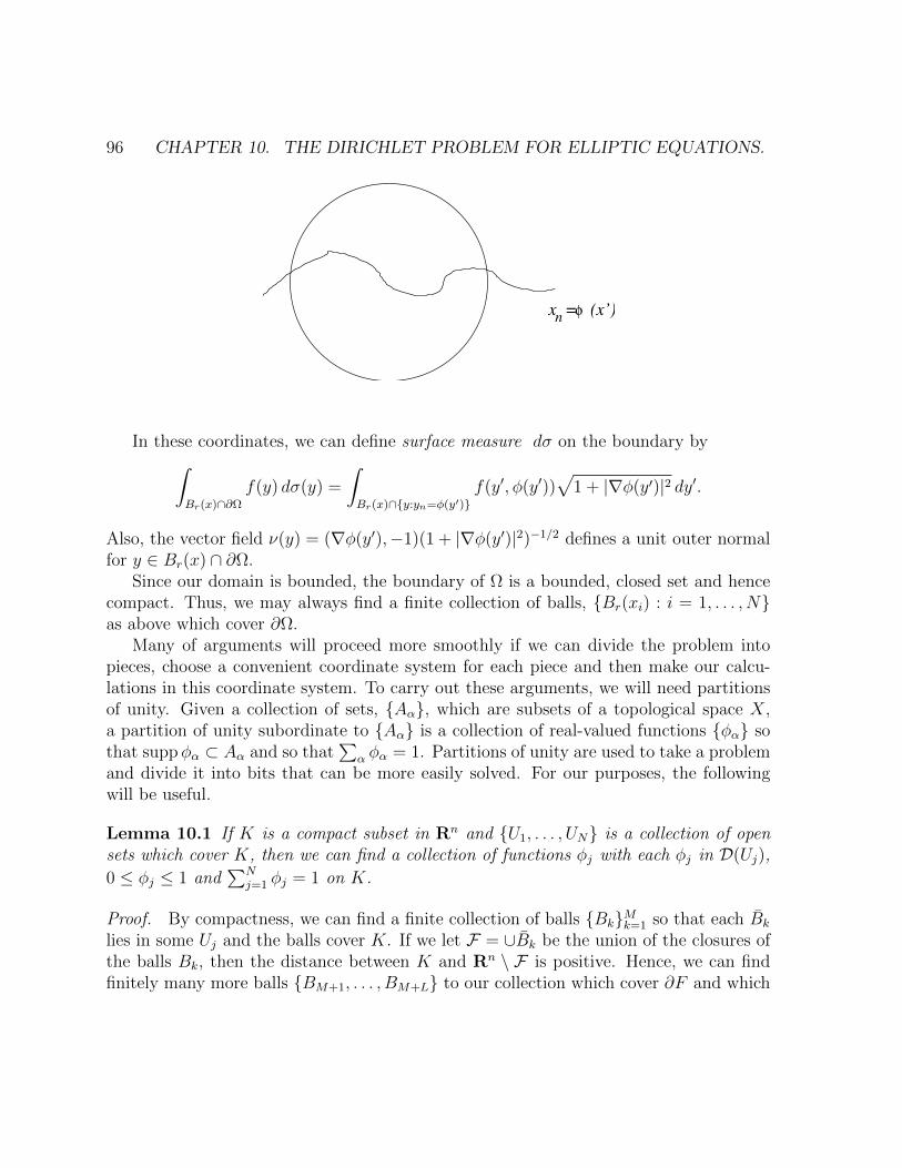
96 CHAPTER 10. THE DIRICHLET PROBLEM FOR ELLIPTIC EQUATIONS.

x = (x’)φn

In these coordinates, we can define surface measure dσ on the boundary by∫Br(x)∩∂Ω

f(y) dσ(y) =

∫Br(x)∩y:yn=φ(y′)

f(y′, φ(y′))√

1 + |∇φ(y′)|2 dy′.

Also, the vector field ν(y) = (∇φ(y′),−1)(1 + |∇φ(y′)|2)−1/2 defines a unit outer normalfor y ∈ Br(x) ∩ ∂Ω.

Since our domain is bounded, the boundary of Ω is a bounded, closed set and hencecompact. Thus, we may always find a finite collection of balls, Br(xi) : i = 1, . . . , Nas above which cover ∂Ω.

Many of arguments will proceed more smoothly if we can divide the problem intopieces, choose a convenient coordinate system for each piece and then make our calcu-lations in this coordinate system. To carry out these arguments, we will need partitionsof unity. Given a collection of sets, Aα, which are subsets of a topological space X,a partition of unity subordinate to Aα is a collection of real-valued functions φα sothat suppφα ⊂ Aα and so that

∑α φα = 1. Partitions of unity are used to take a problem

and divide it into bits that can be more easily solved. For our purposes, the followingwill be useful.

Lemma 10.1 If K is a compact subset in Rn and U1, . . . , UN is a collection of opensets which cover K, then we can find a collection of functions φj with each φj in D(Uj),

0 ≤ φj ≤ 1 and∑N

j=1 φj = 1 on K.

Proof. By compactness, we can find a finite collection of balls BkMk=1 so that each Bk

lies in some Uj and the balls cover K. If we let F = ∪Bk be the union of the closures ofthe balls Bk, then the distance between K and Rn \ F is positive. Hence, we can findfinitely many more balls BM+1, . . . , BM+L to our collection which cover ∂F and which

10.1. DOMAINS IN RN 97

are contained in Rn \K. We now let ηk be the standard bump translated and rescaledto the ball Bk. Thus if Bk = Br(x), then ηk(y) = exp(−1/(r2 − |y − x|2)) in Bk and 0outside Bk. Finally, we put η =

∑M+Lk=1 ηk and then ηk = ηk/η. Each ηk, k = 1, . . . ,M is

smooth since η is strictly positive on O. Then we have∑M

k=1 ηk = 1 on K and we maygroup to obtain one φj for each Uj.

The following important result is the Gauss divergence theorem. Recall that for a Cn

valued function F = (F1, . . . , Fn), the divergence of F , is defined by

divF =n∑j=1

∂Fj∂xj

.

Theorem 10.2 (Gauss divergence theorem) Let Ω be a C1 domain and let F : Ω→ Cn

be in C1(Ω). We have ∫∂Ω

F (x) · ν(x) dσ(x) =

∫Ω

divF (x) dx.

The importance of this result may be gauged by the following observation: the theoryof weak solutions of elliptic pde (and much of distribution theory) relies on making thisresult an axiom.

An important Corollary is the following version of Green’s identity. In this Corollaryand below, we should visualize the gradient of u, ∇u as a column vector so that theproduct A∇u is makes sense as a matrix product.

Corollary 10.3 If Ω is a C1-domain, v is in C1(Ω), u is in C2(Ω) and A(x) is an n×nmatrix with C1(Ω) entries, then∫

∂Ω

v(x)A(x)∇u(x) · ν(x) dσ(x) =

∫Ω

A(x)∇u(x) · ∇v(x) + v(x) divA(x)∇u(x) dx.

Proof. Apply the divergence theorem to vA∇u.

Next, we define Sobolev spaces on open subsets of Rn. Our definition is motivated bythe result in Proposition 3.13. For k a positive integer, we say that u ∈ L2,k(Ω) if u hasweak or distributional derivatives for all α for |α| ≤ k and these derivatives, ∂αu/∂xα,lie in L2(Ω). This means that for all test functions φ ∈ D(Ω), we have∫

Ω

u∂α

∂xαφ(x) dx = (−1)|α|

∫Ω

φ∂α

∂xαu(x) dx.


The weak derivatives of u are defined as we defined the derivatives of a tempered dis-tribution. The differences are that since we are on a bounded open set, our functionsare supported there and in this instance we require that the derivative be a distributiongiven by a function.

It should be clear how to define the norm in this space. In fact, we have that thesespaces are Hilbert spaces with the inner product defined by

〈u, v〉 =

∫Ω

∑|α|≤k

∂αu

∂xα∂αv

∂xαdx. (10.4)

We let ‖u‖L2,k(Ω) be the corresponding norm.

Exercise 10.5 Show that if Ω is a bounded open set, then Ck(Ω) ⊂ L2,k(Ω).

Example 10.6 If u is in the Sobolev space L2,k(Rn) defined in Chapter 3 and Ω is anopen set, then the restriction of u to Ω, call it ru, is in the Sobolev space L2,k(Ω). If Ωhas reasonable boundary, (C1 will do) then the restriction map r : L2,k(Rn)→ L2,k(Ω) isonto. However, this may fail in general.

Exercise 10.7 a) Prove the product rule for weak derivatives. If φ is in Ck(Ω) and allthe derivatives of φ, ∂αφ/∂xα with |α| ≤ k are bounded, then we have that

∂αφu

∂xα=∑

β+γ=α

α!

β!γ!

∂βφ

∂xβ∂γu

∂xγ.

b)If φ ∈ Ck(Ω), conclude that the map u → φu takes L2,k(Ω) to L2,k(Ω) and isbounded.

c) If φ ∈ C1(Ω), show that the map u→ φu maps L2,10 (Ω)→ L2,1

0 (Ω).

Lemma 10.8 If Ω is a C1 domain and u is in the Sobolev space L2,k(Ω), then we maywrite u =

∑Nj=0 uj where u0 has support in a fixed (independent of u) compact subset

of Ω and each uj, j = 1, . . . , N is supported in a ball Brj(xj) as in the definition of C1

domain.

Proof. We cover the boundary, ∂Ω by balls B1, . . . , BN as in the definition of C1

domain. Then, K = Ω\∪Nk=1Bk is a compact set so that the distance from K to Rn \Ω ispositive, call this distance δ. Thus, we can find an open set U0 = x : dist(x, ∂Ω) > δ/2which contains K and is a positive distance from ∂Ω. We use Lemma 10.1 to make apartition of unity 1 =

∑Nj=0 ηj for the open cover of Ω U0, B1 . . . , BN and then we

decompose u =∑N

j=0 ηju . The product rule of exercise 10.7 allows us to conclude that

each term uj = ηju is in L2,k(Ω).

Recall that we proved in Chapter 2 that smooth (Schwartz, actually) functions aredense in Lp(Rn), 1 ≤ p <∞. One step of the argument involved considering the map

η ∗ u

where η is a Schwartz function with∫η = 1. This approach may appear to break down

u is only defined in an open subset of Rn, rather than all of Rn. However, we can makesense of the convolution in most of Ω if we require that the function η have compactsupport. Thus, we let η ∈ D(Rn) be supported in B1(0) and have

∫η = 1.

Lemma 10.9 Suppose u is the Sobolev space Lp,k(Ω), 1 ≤ p < ∞, for k = 0, 1, 2, . . . .Set Ωε = Ω ∩ x : dist(x, ∂Ω) > ε. If we set uδ = ηδ ∗ u, then for |α| ≤ k, we have

∂α

∂xαuδ = (

∂α

∂xαu)δ, for x ∈ Ωε with δ < ε.

Hence, for each ε > 0, we have

limδ→0+

‖u− uδ‖Lp,k(Ωε) = 0.

Proof. We assume that u is defined to be zero outside of Ω. The convolution u ∗ ηδ(x)is smooth in all of Rn and we may differentiate inside the integral and then express thex derivatives as y derivatives to find

∂α

∂xαu ∗ ηδ(x) =

∫Ω

u(y)∂α

∂xαηδ(x− y) dy = (−1)|α|

∫Ω

u(y)∂α

∂yαηδ(x− y) dy.

If we have δ < ε and x ∈ Ωε, then ηδ(x − ·) will be in the space of test functions D(Ω).Thus, we can apply the definition of weak derivative to conclude

(−1)|α|∫

Ω

u(y)∂α

∂yαηδ(x− y) dy =

∫Ω

(∂α

∂yαu(y))ηδ(x− y) dy.

Lemma 10.10 If Ω is a C1-domain and k = 0, 1, 2, . . . , then C∞(Ω) is dense in L2,k(Ω).

Proof. We may use Lemma 10.8 to reduce to the case when u is zero outside Br(x)∩Ωfor some ball centered at a boundary point x and ∂Ω is given as a graph, (x′, xn) : xn =φ(x′) in Br(x). We may translate u to obtain uε(x) = u(x + εen). Since uε has weakderivatives in a neighborhood of Ω, by the local approximation lemma, Lemma 10.9 wemay approximate each uε by functions which are smooth up to the boundary of Ω.

Lemma 10.11 If Ω and Ω′ are bounded open sets and F : Ω → Ω′ is C1(Ω) and F−1 :Ω′ → Ω is also C1(Ω′), then we have u ∈ L2,1(Ω′) if and only if u F ∈ L2,1(Ω).

Proof. The result is true for smooth functions by the chain rule and the change ofvariables formulas of vector calculus. Note that our hypothesis that F is invertibleimplies that the Jacobian is bounded above and below. The density result of Lemma10.9 allows us to extend to the Sobolev space.

Lemma 10.12 If Ω is a C1-domain, then there exists an extension operator E : L2,k(Ω)→L2,k(Rn).

Proof. We sketch a proof when k = 1. We will not use the more general result. Thegeneral result requires a more substantial proof. See the book of Stein [29], whose resulthas the remarkable feature that the extension operator is independent of k.

For the case k = 1, we may use a partition of unity and to reduce to the case where uis nonzero outside Br(x)∩Ω and that ∂Ω is the graph (x′, xn) : xn = φ(x′) in Br(x). Bythe density result, Lemma 10.10, we may assume that u is smooth up to the boundary.Then we can define Eu by

Eu(x) =

u(x), xn > φ(x′)u(x′, 2φ(x′)− xn), xn < φ(x′)

If ψ is test function in Rn, then we can apply the divergence theorem in Ω and inRn \ Ω to obtain that ∫

Ω

Eu∂ψ

∂xj+ ψ

∂Eu

∂xjdx =

∫∂Ω

ψEuν · ej dσ∫Rn\Ω

Eu∂ψ

∂xj+ ψ

∂Eu

∂xjdx = −

∫∂Ω

ψEuν · ej dσ

In the above expressions, the difference in sign is due to the fact that the normal whichpoints out of Ω is the negative of the normal which points out of Rn \ Ω.

Adding these two expressions, we see that Eu has weak derivatives in Rn. These weakderivatives are given by the (ordinary) derivative ∂Eu/∂xj, which is defined except on∂Ω. In general, Eu will not have an ordinary derivative on ∂Ω. Using Lemma 10.11, onecan see that this extension operator is bounded. The full extension operator is obtainedby taking a function u, writing u =

∑Nj=0 ηju as in Lemma 10.8 where the support of η0

does not meet the boundary. For each ηj which meets the boundary, we apply the local


extension operator constructed above and then sum to obtain Eu = η0u+∑N

j=1E(ηju).

Once we have defined the extension operator on smooth functions in L2,1, then we canuse the density result of Lemma 10.10 to define the extension operator on the full space.

Next, we define an important subspace of L2,1(Ω), L2,10 (Ω). This space is the closure

of D(Ω) in the norm of L2,1(Ω). The functions in L2,10 (Ω) will be defined to be the

Sobolev functions which vanish on the boundary. Since a function u in the Sobolev spaceis initially defined a.e., it should not be clear that we can define the restriction of u to alower dimensional subset. However, we saw in Chapter 9 that this is possible. We shallpresent a second proof below. The space L2,1

0 (Ω) will be defined as the space of functionswhich have zero boundary values.

Remark: Some of you may be familiar with the spaces L2,1(Ω) as H1(Ω) and L2,10 (Ω)

as H10 (Ω).

We define the boundary values of a function in L2,1(Ω) in the following way. Wesay that u = v on ∂Ω if u − v ∈ L2,1

0 (Ω). Next, we define a space L2,1/2(∂Ω) to be theequivalence classes [u] = u+L2,1

0 (Ω) = v : v− u ∈ L2,1(Ω). Of course, we need a normto do analysis. The norm is given by

‖u‖L2,1/2(∂Ω) = inf‖v‖L2,1(Ω) : u− v ∈ L2,10 (Ω). (10.13)

It is easy to see that this is a norm and the resulting space is a Banach space. It isless clear L2,1/2(∂Ω) is a Hilbert space. However, if the reader will recall the proof ofthe projection theorem in Hilbert space one may see that the space on the boundary,L2,1/2(∂Ω), can be identified with the orthogonal complement of L2,1

0 (Ω) in L2,1(Ω) andthus inherits an inner product from L2,1(Ω).

This way of defining functions on the boundary should be unsatisfyingly abstract tothe analysts in the audience. The following result gives a concrete realization of thespace.

Proposition 10.14 Let Ω be a C1-domain. The map

r : C1(Ω)→ L2(∂Ω)

which takes φ to the restriction of φ to the boundary, rφ satisfies

‖ru‖L2(∂Ω) ≤ C‖u‖L2,1(Ω)

and as a consequence extends continuously to L2,1(Ω). Since r(L2,10 (Ω)) = 0, the map

r is well-defined on equivalence classes in L2,1/2(∂Ω) and gives a continuous injectionr : L2,1/2(∂Ω)→ L2(∂Ω).


Exercise 10.15 Prove the above proposition.

Exercise 10.16 If Ω is a C1 domain, let H be a space of functions f on ∂Ω defined asfollows. We say that f ∈ H if for each ball Br(x) as in the definition of C1 domains andeach η ∈ D(Br(x)), we have (ηf)(y′, φ(y′)) is in the space L2,1/2(Rn−1) defined in Chapter3. In the above, φ is the function whose graph describes the boundary of Ω near x. Anorm in the space H may be defined by fixing a covering of the boundary by balls as inthe definition of C1-domains, and then a partition of unity subordinate to this collectionof balls,

∑ηk and finally taking the sum∑

k

‖ηkf‖L2,1/2(Rn−1)

.Show that H = L2,1/2(∂Ω).Hint: We do not have the tools to solve this problem. Thus this exercise is an excuse

to indicate the connection without providing proofs.

Lemma 10.17 If Ω is a C1 domain and u ∈ C1(Ω), then there is a constant C so that∫∂Ω

|u(x)|2 dσ(x) ≤ C

∫Ω

|u(x)|2 + |∇u(x)|2 dx.

Proof. According to the definition of a C1-domain, we can find a finite collection of ballsBj : j = 1, . . . , N and in each of these balls, a unit vector, αj, which satisfies αj · ν ≥δ > 0 for some constant δ. To do this, choose αj to be −en in the coordinate system whichis used to describe the boundary near Bj. The lower bound will be minj(1+‖∇φj‖2

∞)−1/2

where φj is the function which defines the boundary near Bj. Using a partition of unity∑j φj subordinate to the family of balls Bj which is 1 on ∂Ω, we construct a vector field

α(x) =N∑j=1

φj(x)αj.

We have α(x) · ν(x) ≥ δ since each αj satisfies this condition and each φj takes values in[0, 1]. Thus, the divergence theorem gives

δ

∫∂Ω

|u(x)|2 dσ(x) ≤∫∂Ω

|u(x)|2α(x) · ν(x) dx

=

∫Ω

|u|2( divα) + 2 Re(u(x)α · ∇u(x)) dx.

Applying the Cauchy-Schwarz inequality proves the inequality of the Lemma. The con-stant depends on Ω through the vector field α and its derivatives.

10.2. THE WEAK DIRICHLET PROBLEM 103

Proof of Proposition 10.14. The proposition follows from the lemma. That the map rcan be extended from nice functions to all of L2,1(Ω) depends on Lemma 10.10 whichasserts that nice functions are dense in L2,1(Ω).

Exercise 10.18 Suppose that Ω is a C1 domain. Show that if φ ∈ C1(Ω) and φ(x) = 0on ∂Ω, then φ(x) is in the Sobolev space L2,1

0 (Ω).

Finally, we extend the definition of one of the Sobolev spaces of negative order todomains. We define L2,−1(Ω) to be the dual of the space L2,1

0 (Ω). As in the case of Rn,the following simple lemma gives examples of elements in this space.

Proposition 10.19 Assume Ω is an open set of finite measure, and g and f1, . . . , fn arefunctions in L2(Ω). Then

φ→ λ(φ) =

∫Ω

g(x)φ(x) +n∑j=1

fj(x)∂φ(x)

∂xjdx

is in L2,−1(Ω).

Proof. According to the Cauchy-Schwarz inequality, we have

λ(φ) ≤(∫

Ω

|u(x)|2 + |∇u(x)|2 dx)1/2

(∫Ω

|g(x)|2 + |n∑j=1

fj(x)2| dx

)1/2

.

10.2 The weak Dirichlet problem

In this section, we introduce elliptic operators. We let A(x) be function defined on anopen set Ω and we assume that this function takes values in n × n-matrices with realentries. We assume that each entry is Lebesgue measurable and that A satisfies thesymmetry condition

At = A (10.20)

and ellipticity condition, for some λ > 0,

λ|ξ|2 ≤ A(x)ξ · ξ ≤ λ−1|ξ|2, ξ ∈ Rn, x ∈ Ω. (10.21)


We say that u is a local weak solution of the equation divA(x)∇u = f for f ∈ L2,−1(Ω)if u is in L2,1

loc(Ω) and for all test functions φ ∈ D(Ω), we have

−∫

Ω

A(x)∇u(x) · ∇φ(x) dx = f(φ).

Since the derivatives of u are locally in L2, we can extend to test functions φ which arein L2,1

0 (Ω) and which (have a representative) which vanishes outside a compact subset ofΩ. However, let us resist the urge to introduce yet another space.

Statement of the Dirichlet problem. The weak formulation of the Dirichlet problemis the following. Let g ∈ L2,1(Ω) and f ∈ L2,−1(Ω), then we say that u is a solution ofthe Dirichlet problem if the following two conditions hold:

u ∈ L2,1(Ω) (10.22)

u− g ∈ L2,10 (Ω) (10.23)

−∫

Ω

A(x)∇u(x)∇φ(x) dx = f(φ) φ ∈ L2,10 (Ω). (10.24)

Note that both sides of the equation (10.24) are continuous in φ in the topology ofL2,1

0 (Ω). Thus, we only need to require that this hold for φ in a dense subset of L2,10 (Ω).

A more traditional way of writing the Dirichlet problem is, given g and f find u whichsatisfies

divA∇u = f, in Ωu = g, on ∂Ω

Our condition (10.24) is a restatement of the equation, divA∇u = f . The condition(10.23) is a restatement of the boundary condition u = f . Finally, the condition (10.22)is needed to show that the solution is unique.

Theorem 10.25 If Ω is an open set of finite measure and g ∈ L2,1(Ω) and f ∈ L2,−1(Ω),then there is exactly one weak solution to the Dirichlet problem, (10.22-10.24). There isa constant C(λ, n,Ω) so that the solution u satisfies

‖u‖L2,1(Ω) ≤ C(‖g‖L2,1(Ω) + ‖f‖L2,−1(Ω)).

Proof. Existence. If u ∈ L2,10 (Ω) and n ≥ 3 then Holder’s inequality and then the

Sobolev inequality of Theorem 8.22 imply∫Ω

|u(x)|2 dx ≤(∫

Ω

|u(x)|2nn−2 dx

)1− 2n

m(Ω)2/n ≤ Cm(Ω)2/n

∫Ω

|∇u(x)|2 dx.


If n = 2, the same result holds, though we need to be a bit more persistent and useHolder’s inequality, the Soboleve inequality and Holder again to obtain:∫

Ω

|u(x)|2 dx ≤(∫

Ω

|u(x)|4 dx)1/2

m(Ω)1/2 ≤(∫

Ω

|∇u(x)|4/3 dx)3/2

m(Ω)1/2

≤∫

Ω

|∇u(x)|2 dx m(Ω).

Note that in each case, the application of the Sobolev inequality on Rn is allowed becauseL2,1

0 (Ω) may be viewed as a subspace of L2,1(Ω) by extending functions on Ω to be zerooutside Ω. Thus we have

‖u‖L2(Ω) ≤ Cm(Ω)1/n‖∇u‖L2(Ω). (10.26)

Next, we observe that the ellipticity condition (10.21) implies that

λ

∫Ω

|∇u(x)|2 ≤∫

Ω

A(x)∇u(x)∇u(x) dx ≤ λ−1

∫Ω

|∇u(x)|2 dx. (10.27)

We claim the expression ∫Ω

A(x)∇u(x)∇v(x) dx (10.28)

provides an inner product on L2,10 (Ω) which induces the same topology as the standard

inner product on L2,10 (Ω) ⊂ L2,1(Ω) defined in (10.4). To see that the topologies are the

same, it suffices to establish the inequalities∫Ω

|∇u(x)|2 + |u(x)|2 dx ≤ λ−1(1 + Cm(Ω)2/n)

∫Ω

A(x)∇u(x)∇u(x) dx

and that∫Ω

A(x)∇u(x)∇u(x) dx ≤ λ−1

∫Ω

|∇u(x)|2 dx ≤ λ−1

∫Ω

|∇u(x)|2 + |u(x)|2 dx.

These both follow from the estimates (10.26) and (10.27). As a consequence, standardHilbert space theory tells us that any continuous linear functional on L2,1

0 (Ω) can berepresented using the inner product defined in (10.28). We apply this to the functional

φ→ −∫

Ω

A∇g∇φ dx− f(φ)


and conclude that there exists v ∈ L2,10 (Ω) so that∫

Ω

A(x)∇v(x)∇φ(x) dx = −∫

Ω

A(x)∇g(x)∇φ(x) dx− f(φ), φ ∈ L21,0(Ω). (10.29)

Rearranging this expression, we can see that u = g+v is a weak solution to the Dirichletproblem.

Uniqueness. If we have two solutions of the Dirichlet problem u1 and u2, then theirdifference w = u1 − u2 is a weak solution of the Dirichlet problem with f = g = 0. Inparticular, w is in L2,1

0 (Ω) and we can use w as a test function and conclude that∫A(x)∇w(x) · ∇w(x) dx = 0.

Thanks to the inequalities (10.26) and (10.27) we conclude that∫Ω

|w(x)|2 dx = 0.

Hence, u1 = u2.Stability. Finally, we establish the estimate for the solution. We replace the test

function φ in (10.29) by v. Using the Cauchy-Schwarz inequality gives∫Ω

A∇v · ∇v dx ≤ λ−1‖v‖L2,10 (Ω)‖∇g‖L2,1(Ω) + ‖f‖L2,−1(Ω)‖v‖L2,1

0 (Ω).

If we use that the left-hand side of this inequality is equivalent with the norm in L2,10 (Ω),

cancel the common factor, we obtain that

‖v‖L2,10 (Ω) ≤ C‖g‖L2,1

0 (Ω) + ‖f‖L2,−1(Ω).

We have u = v + g and the triangle inequality gives

‖u‖L2,1(Ω) ≤ ‖g‖L2,1(Ω) + ‖v‖L2,10 (Ω)

so combining the last two inequalities implies the estimate of the theorem.

Exercise 10.30 (Dirichlet’s principle.) Let g ∈ L2,1(Ω) and suppose that f = 0 in theweak formulation of the Dirichlet problem.

a) Show that the expression

I(u) =

∫Ω

A(x)∇u(x) · ∇u(x) dx


attains a minimum value on the set g + L2,10 (Ω) = g + v : v ∈ L2,1

0 (Ω). Hint: Use thefoil method. This is a general fact in Hilbert space.

b) If u is a minimizer for I, then u is a weak solution of the Dirichlet problem,divA∇u = 0 and u = g on the boundary.

c) Can you extend this approach to solve the general Dirichlet problem divA∇u = fin Ω and u = g on the boundary?

Chapter 11

Inverse Problems: Boundaryidentifiability

11.1 The Dirichlet to Neumann map

In this section, we introduce the Dirichlet to Neumann map. Recall the space L2,1/2(∂Ω)which was introduced in Chapter 10. We let Ω be a bounded open set, A a matrix whichsatisfies the ellipticity condition and given f in L2,1/2(∂Ω), we let u = uf be the weaksolution of the Dirichlet problem

divA∇u = 0, on Ωu = f, on ∂Ω.

(11.1)

Given u ∈ L2,1(Ω) we can define a continuous linear functional on L2,1(Ω) by

φ→∫

Ω

A(x)∇u(x)∇φ(x) dx.

If we recall the Green’s identity (10.3), we see that if u and A are smooth, then∫∂Ω

A(x)∇u(x) · ν(x)φ(x) dσ(x) =

∫Ω

A(x)∇u(x)∇φ(x) + φ(x) divA(x)∇u(x) dx.

Thus, if u solves the equation divA∇u = 0, then it reasonable to define A∇u · ν as alinear functional on L2,1/2(∂Ω) by

A∇u · ν(φ) =

∫Ω

A(x)∇u(x) · ∇φ(x) dx. (11.2)

109

110 CHAPTER 11. INVERSE PROBLEMS: BOUNDARY IDENTIFIABILITY

We will show that this map is defined on L2,1/2(∂Ω) The expression A∇u · ν is called theconormal derivative of u at the boundary. Note that it is something of a miracle that wecan make sense of this expression at the boundary. To appreciate that this is surprising,observe that we are not asserting that the full gradient of u is defined at the boundary,only the particular component A∇u · ν. The gradient of u may only be in L2,(Ω) andthus there is no reason to expect that any expression involving ∇u could make sense onthe boundary, a set of measure zero.

A potential problem is that this definition may depend on the representative of φwhich is used to define the right-hand side of (11.2). Fortunately, this is not the case.

Lemma 11.3 If u ∈ L2,1(Ω) and u is a weak solution of divA∇u = 0, then the value ofA∇u · ν(φ) is independent of the extension of φ from ∂Ω to Ω.

The linear functional defined in (11.2) is a continuous linear functional on L2,1/2(∂Ω).

Proof. To establish that A∇u · ν is well defined, we will use that u is a solution ofdivA∇u = 0. We choose φ1, φ2 in L2,1(Ω) and suppose φ1 − φ2 ∈ L2,1

0 (Ω). According tothe definition of weak solution,∫

Ω

A(x)∇u(x) · ∇(φ1(x)− φ2(x)) dx = 0.

To establish the continuity, we need to choose a representative of φ which is close tothe infinum in the definition of the L2,1/2-norm (see (10.13)). Thus we need ‖φ‖L2,1(Ω) ≤2‖rφ‖L2,1/2(∂Ω). Here, rφ denotes the restriction of φ to the boundary. With this choiceof φ and Cauchy-Schwarz we have

|A∇u · ν(φ)| ≤ C‖∇u‖L2(Ω)‖∇φ‖L2(Ω).

This inequality implies the continuity.

We will define L2,−1/2(∂Ω) as the dual of the space L2,1/2(∂Ω). Now, we are ready todefine the Dirichlet to Neumann map. This is a map

ΛA : L2,1/2(Ω)→ L2,−1/2(∂Ω)

defined byΛAf = A∇u · ν

where u is the solution of the Dirichlet problem with boundary data f .The traditional goal in pde is to consider the direct problem. For example, given

the coefficient matrix A, show that we can solve the Dirichlet problem. If we were more

11.1. THE DIRICHLET TO NEUMANN MAP 111

persistent, we could establish additional properties of the solution. For example, we couldshow that the map A→ ΛA is continuous, on the set of strictly positive definite matrixvalued functions on Ω.

However, that would be the easy way out. The more interesting and difficult problemis the inverse problem. Given the map ΛA, can we recover the coefficient matrix, A. Thatis given some information about the solutions to a pde, can we recover the equation. Theanswer to the problem, as stated, is no, of course not.

Exercise 11.4 Let Ω be a bounded domain and let F : Ω→ Ω be a C1(Ω) diffeomorphismthat fixes a neighborhood of the boundary. Show that if A gives an elliptic operator divA∇on Ω, then there is an operator divB∇ so that

divA∇u = 0 ⇐⇒ divB∇u F = 0.

As a consequence, it is clear that the maps ΛA = ΛB. Hint: See Lemma 11.10 below forthe answer.

Exercise 11.5 Show that the only obstruction to uniqueness is the change of variablesdescribed in the previous problem.

Remark: This has been solved in two dimensions, by John Sylvester [35]. In threedimensions and above, this problem is open.

Exercise 11.6 Prove that the map A→ ΛA is continuous on the set of strictly positivedefinite and bounded matrix-valued functions. That is show that

‖ΛA − ΛB‖L(L2,1/2,L2,−1/2) ≤ Cλ‖A−B‖∞.

Here, ‖ · ‖L(L2,1/2,L2,−1/2) denotes the norm on linear operators from L2,1/2 to L2,−1/2.

a) As a first step, show that if we let uA and uB satisfy divA∇uA = divB∇uB = 0in an open set Ω and uA = uB = f on ∂Ω, then we have∫

Ω

|∇uA −∇uB|2 dx ≤ C‖f‖L2,1/2(∂Ω)‖A−B‖2∞.

Hint: We have divB∇uA = div (B − A)∇uA since uA is a solution.

b) Conclude the estimate above on the Dirichlet to Neumann maps.


However, there is a restricted version of the inverse problem which can be solved. Inthe remainder of these notes, we will concentrate on elliptic operators when the matrixA is of the form A(x) = γ(x)I where I is the n× n identity matrix and γ(x) is a scalarfunction which satisfies

λ ≤ γ(x) ≤ λ−1 (11.7)

for some constant λ > 0. We change notation a bit and let Λγ be the Dirichlet toNeumann map for the operator div γ∇. Then the inverse conductivity problem can beformulated as the following question:

Is the map γ → Λγ injective?

We will answer this question with a yes, if the dimension n ≥ 3 and we have some rea-sonable smoothness assumptions on the domain and γ. This is a theorem of J. Sylvesterand G. Uhlmann [36]. The following year, closely related work was done by Henkin andR. Novikov [17, 23]. One can also ask for a more or less explicit construcion of the inversemap. A construction is given in in the work of Novikov and the work of A. Nachman[22] for three dimensions and [21] in two dimensions. This last paper also gives the firstproof of injectivity in two dimensions. My favorite contribution to this story is in [9].But this is not the the place for a complete history.

We take a moment to explain the appearance of the word conductivity in the above.For this discussion, we will assume that function u and γ are smooth. The problem weare considering is a mathematical model for the problem of determining the conductivityγ by making measurements of current and voltage at the boundary. To try and explainthis, we suppose that u represents the voltage potential in Ω and then ∇u is the electricfield. The electric field is what makes electrons flow and thus we assume that the currentis proportional to the electric field, J = γ∇u where the conductivity γ is a constant ofproportionality. Since we assume that charge is conserved, for each subregion B ⊂ Ω,the net flow of electrons or current through B must be zero. Thus,

0 =

∫∂B

γ∇u(x) · ν(x) dσ(x).

The divergence theorem gives that

0 =

∫∂B

γ(x)∇u(x) · ν(x) dσ(x) =

∫B

div γ(x)∇u(x) dx.

Finally, since the integral on the right vanishes, say, for each ball B ⊂ Ω, we can concludethat div γ∇u = 0 in Ω.

11.2. IDENTIFIABILITY 113

11.2 Identifiability

Our solution of the inverse conductivity problem has two steps. The first is to show thatthe Dirichlet to Neumann map determines γ on the boundary. The second step is touse the knowledge of γ on the boundary to relate the inverse conductivity problem to aproblem in all of Rn which turns out to be a type of scattering problem. We will use theresults of Chapter 9 to study this problem in Rn.

Theorem 11.8 Suppose that ∂Ω is C1. If γ is in C0(Ω) and satisfies (11.7), then foreach x ∈ ∂Ω, there exists a sequence of functions uN so that

γ(x) = limN→∞

ΛγuN(uN).

Theorem 11.9 Suppose Ω and γ are as in the previous theorem and also ∂Ω is C2 andγ is in C1(Ω). If e is a constant vector and uN as in the previous theorem, then we have

∇γ(x) · e = limN→∞

∫∂Ω

(γ(x)|∇uN(x)|2e · ν(x)− 2 Re γ(x)

∂uN∂ν

(x)e · ∇u(x)

)dσ.

The construction of the solutions uN proceeds in two steps. The first step is to writedown an explicit function which is an approximate solution and show that the conclusionof our Theorem holds for this function. The second step is to show that we really do havean approximate solution. This is not deep, but requires a certain amount of persistence.I say that the result is not deep because it relies only on estimates which are a byproductof our existence theory in Theorem 10.25.

In the construction of the solution, it will be convenient to change coordinates so thatin the new coordinates, the boundary is flat. The following lemma keeps track of howthe operator div γ∇ transforms under a change of variables.

Lemma 11.10 Let A be an elliptic matrix and F : Ω′ → Ω be a C1(Ω′)-diffeomorphism.We have that divA∇u = 0 if and only if divB∇u F where

B(y) = | detDF (y)|DF−1(F (y))tA(F (y))DF−1(F (y)).

Proof. The proof of this lemma indicates one of the advantages of the weak formulationof the equation. Since the weak formulation only involves one derivative, we only needto use the chain rule once.

We use the chain rule to compute

∇u(x) = ∇(u(F (F−1(x))) = DF−1(x)∇(u F )(F−1(x)).


This is valid for Sobolev functions also by approximation (see Lemma 10.11). We insertthis expression for the gradient and make a change of variables x = F (y) to obtain∫

Ω

A(x)∇u(x) · ∇φ(x) dx

=

∫Ω′A(F (y))DF−1(F (y))∇(u F (y)) ·DF−1(F (y))∇(φ F (y))| detDF (y)| dy

=

∫Ω′| detDF (y)|DF−1(F (y))tA(F (y))DF−1(F (y))∇(u F (y)) · ∇(φ F (y)) dy.

This last integral is the weak formulation of the equation divB∇u = 0 with the testfunction φ F . To finish the proof, one must convince oneself that the map φ → φ Fis an isomorphism1 from L2,1

0 (Ω) to L2,10 (Ω′).

Exercise 11.11 Figure out how to index the matrix DF−1 so that in the application ofthe chain rule in the previous Lemma, the product DF−1∇(uF ) is matrix multiplication.Assume that the gradient is a column vector.

Solution The chain rule reads

∂

∂xiu G =

∂Gj

∂xi

∂u

∂xjG.

Thus, we want

(DG)ij =∂Gj

∂xi.

In the rest of this chapter, we fix a point x on the boundary and choose coordinatesso that x is the origin. Thus, we suppose that we are trying to find the value of γand ∇γ at 0. We assume that ∂Ω is C1 near 0 and thus we have a ball Br(0) so thatB2r(0) ∩ ∂Ω = (x′, xn) : xn = φ(x′) ∩ B2r(0). We let x = F (y′, yn) = (y′, φ(y′) + yn).Note that we assume that the function φ is defined in all of Rn−1 and thus, the map F isinvertible on all of Rn. In the coordinates, (y′, yn), the operator div γ∇ takes the form

divA∇u = 0

with A(y) = γ(y)B(y). (Strictly speaking, this is γ(F (y)). However, to simplify thenotation, we will use γ(z) to represent the value of γ at the point corresponding to z

1An isomorphism for Banach (or Hilbert spaces) is an invertible linear map with continuous inverse.A map which also preserves the norm is called an isometry.

in the current coordinate system. This is a fairly common convention. To carry it outprecisely would require yet another chapter that we don’t have time for...) The matrixB depends on φ and, by the above lemma, takes the form

B(y) =

(1n−1 −∇φ(y′)

−∇φ(y′)t 1 + |∇φ(y′)|2).

Apparently, we are writing the gradient as a column vector. The domain Ω′ has 0 on theboundary and near 0, ∂Ω′ lies in the hyperplane yn = 0 and Ω′ lies in the regions yn > 0.We introduce a real-valued cutoff function η(y) = f(y′)g(yn) where f is supported in|y′| < 2 and is normalized so that ∫

Rn−1

f(y′)2 dy′ = 1 (11.12)

and so that g(yn) = 1 if |yn| < 1 and g(yn) = 0 if |yn| > 2. Our next step is to setηN(x) = N (n−1)/4η(N1/2y). We choose a vector α ∈ Rn and which satisfies

B(0)α · en = 0 (11.13)

B(0)α · α = B(0)en · en. (11.14)

We define EN byEN(y) = N−1/2 exp(−N(yn + iα · y))

and then we putvN(y) = ηN(y)EN(y). (11.15)

The function vN is our approximate solution. The main facts that we need to proveabout vN are Lemma 11.18 and Lemma 11.25 below. Lemma 11.25 asserts that vN is anappoximate solution of an elliptic equation. To visualize why this might be true, observethat EN is a solution of the equation with constant coefficients B(0). The cutoff functionoscillates less rapidly than EN (consider the relative size of the gradients) and thus itintroduces an error that is negligible for N large and allows us to disregard the fact thatEN is not a solution away from the origin.

Our proof will require yet more lemmas. The function vN is concentrated near theboundary. In the course of making estimates, we will need to consider integrals pairingvN and its derivatives against functions which are in L2,1

0 (Ω). To make optimal estimates,we will want to exploit the fact that functions in L2,1

0 (Ω) are small near the boundary.The next estimate, a version of Hardy’s inequality makes this precise. If we have notalready made this definition, then we define

δ(x) = infy∈∂Ω|x− y|.

The function δ gives the distance from x to the boundary of Ω.

Lemma 11.16 (Hardy’s inequality) a) Let f be a C1 function on the real line and sup-pose that f(0) = 0, then for 1 < p ≤ ∞,∫ ∞

0

|f(t)

t|p dt ≤ p′

∫ ∞0

|f ′(t)|p dt.

b) If f is in L2,10 (Ω), then∫

Ω

∣∣∣∣f(x)

δ(x)

∣∣∣∣2 dx ≤ C

∫Ω

|∇f(x)|2 + |f(x)|2 dx.

Proof. a) We prove the one-dimensional result with p <∞ first. We use the fundamentaltheorem of calculus to write

f(t) = −∫ t

0

f ′(s) ds

Now, we confuse the issue by rewriting this as

−t1p−1f(t) =

∫(t/s)−1/p′χ(1,∞)(t/s)s

1/pf(s)ds

s

=

∫K(t/s)s1/pf ′(s)

ds

s(11.17)

where K(u) = u−1/p′χ(1,∞)(u). A computation shows that∫ ∞0

K(t/s)ds

s=

∫ ∞0

K(t/s)dt

t= p′

which will be finite if p > 1. Thus, by exercise 4.5 we have that g →∫K(t/s)g(s) ds/s

maps Lp(ds/s) into itself. Using this in (11.17) gives(∫ ∞0

∣∣∣∣f(t)

t

∣∣∣∣p dt)1/p

≤ p′(∫ ∞

0

|f ′(t)|p dt)1/p

.

Which is what we wanted to prove. The remaining case p =∞ where the Lp norms mustbe replaced by L∞ norms is easy and thus omitted.

b) Since D(Ω) is dense in L2,10 (Ω), it suffices to consider functions in D(Ω). By a

partition of unity, as in Lemma 10.8 we can further reduce to a function f which iscompactly supported Br(x) ∩ Ω, for some ball centered at x on the boundary, or to a

function f which is supported at a fixed distance away from the boundary. In the firstcase have that ∂Ω is given by the graph (y′, yn) : yn = φ(y′) near x. Applying theone-dimensional result in the yn variable and then integrating in the remaining variables,we may conclude that∫

Ω∩Br(x)

|f(y)|2

(yn − φ(y′))2dy ≤ 4

∫Ω∩Br(x)

| ∂u∂yn

(y)|2 dy.

This is the desired inequality once we convince ourselves that (yn−φ(y′))/δ(y) is boundedabove and below in Br(x) ∩ Ω.

The second case where f is supported strictly away from the boundary is an easyconsequence of the Sobolev inequality, Theorem 8.22, because 1/δ(x) is bounded aboveon each compact subset of Ω.

The following Lemma will be useful in obtaining the properties of the approximatesolutions and may serve to explain some of the peculiar normalizations in the definition.

Lemma 11.18 Let vN , EN and ηN be as defined in (11.15). Let β be continuous at 0then

limN→∞

N

∫Ω′β(y)|ηN(y)|2e−2Nyn dy = β(0)/2. (11.19)

If k > −1 and η ∈ D(Rn), then for N sufficiently large there is a constant C so that

|∫

Ω′δ(y)kη(N1/2y)e−2Nyn dy| ≤ CN

1−n2−1−k. (11.20)

Proof. To prove the first statement, we observe that by the definition and the normal-ization of the cutoff function, f , in (11.12) we have that∫

Ω′ηN(y)2e−2Nyn dy = N

n−12

∫y:yn>0

f(N1/2y′)2e−2Nyn dy

+Nn−12

∫y:yn>0

(g(N1/2yn)2 − 1)f(N1/2y′)2e−2Nyn dy.

The first integral is 1/(2) and the second is bounded by a multiple of (2N)−1e−2N1/2.

The estimate of the second depends on our assumption that g(t) = 1 for t < 1. Thus,we have that

limN→∞

N

∫Ω′ηN(y)2e−2Nyndy = 1/2.

Using this to express the 12

as a limit gives

|12β(0)− lim

N→∞N

∫Ω′β(y)ηN(y)2e−2Nyndy| ≤ lim

N→∞N

∫Ω′|β(0)− β(y)|

×ηN(y)2e−2Nyndy

≤ limN→∞

supy:|y|<21/2N−1/2

1

2|β(0)− β(y)|

×N∫

Ω′ηN(y)2e−2Nyndy.

Now the continuity of β implies that this last limit is 0.The inequalities in the second statement follow easily, by observing that for N suffi-

ciently large, we have δ(y) = yn on the support of η(N1/2y). If supp η ⊂ BR(0), then wecan estimate our integral by∣∣∣∣∫

Ω′δ(y)kη(N1/2y)e−2Nyn dy

∣∣∣∣ ≤ ‖η‖∞∫y′:|y′|<N−1/2R

∫ ∞0

ykne−2Nyn dy′dyn

≤ CN1−n2−1−k.

We can now evaluate a limit involving our approximate solution.

Lemma 11.21 With Ω′ and vN as above, suppose β is a bounded function on Ω′ whichis continuous at 0, then

limN→∞

∫Ω′β(y)B(y)∇vN(y) · ∇vN(y) dy = β(0)B(0)en · en.

Proof. Using the product rule, expanding the square and that ηN is real valued gives∫Ω′β(y)B(y)∇vN(y)∇vN(y) dy = N

∫β(y)(B(y)α · α +B(y)en · en)ηN(y)2e−2Nyn dy

−2

∫β(y)(B(y)∇ηN(y) · en)ηN(y)e−2Nyn dy

+N−1

∫Ω′β(y)B(y)∇ηN(y) · ∇ηN(y)e−2Nyn dy

= I + II + III.


By (11.19) of our Lemma 11.18, we have that

limN→∞

I = β(0)(B(0)en · en). (11.22)

where we have used (11.14) to replace B(0)α · α by B(0)en · en. The integral II can bebounded above by

II ≤ 2Nn2 ‖βB‖∞

∫Ω′|(∇η1)(N1/2y)η1(N1/2y)|e−2Nyn dy ≤ CN−1/2. (11.23)

Here, we are using the second part of Lemma 11.18, (11.20). The observant reader willnote that we have taken the norm of the matrix B in the above estimate. The estimateabove holds if matrices are normed with the operator norm–though since we do not careabout the exact value of the constant, it does not matter so much how matrices arenormed.

Finally, the estimate for III also follows from (11.20) in Lemma 11.18 as follows:

III ≤ Nn−12 ‖βB‖∞

∫Ω′|(∇η1)(N1/2y)|2e−2Nyn dy ≤ CN−1. (11.24)

The conclusion of the Lemma follows from (11.22–11.24).

Now, we can make precise our assertion that vN is an approximate solution of theequation divA∇v = 0.

Lemma 11.25 With vN and Ω′ as above,

limN→∞

‖ divA∇vN‖L2,−1(Ω′) = 0.

Proof. We compute and use that divA(0)∇EN = 0 to obtain

divA(y)∇vN(y) = div (A(y)− A(0))∇vN(y) + divA(0)∇vN(y)

= div (A(y)− A(0))∇vN(y)

+2A(0)∇ηN(y)∇EN(y) + EN divA(0)∇ηN(y)

= I + II + III.

In the term I, the divergence must be interpreted as a weak derivative. To estimate thenorm in L2,−1(Ω), we must pair each of I through III with a test function ψ. With I,

we use the definition of weak derivative and recall that ηN is supported in a small ballto obtain

|I(ψ)| =

∣∣∣∣∫ (A(y)− A(0))∇vN(y) · ∇ψ(y) dy

∣∣∣∣≤ sup

|y|<23/2N−1/2

|A(y)− A(0)|‖∇vN‖L2(Ω)‖∇ψ‖L2(Ω).

This last expression goes to zero with N because A is continuous at 0 and according to(11.21) the L2(Ω) of the gradient of vN is bounded as N → 0.

To make estimates for II, we multiply and divide by δ(y), use the Cauchy-Schwarzinequality, the Hardy inequality, Lemma 11.16, and then (11.20)

|II(ψ)| = |∫

Ω′2A(0)∇ηN(y)∇EN(y)ψ(y) dy|

≤

(∫Ω′

∣∣∣∣ψ(y)

δ(y)

∣∣∣∣2 dy)1/2(

Nn+32

∫Ω′δ(y)2|(∇η1)(N1/2y)|2e−2Nyn dy

)1/2

≤ CN−1/2‖ψ‖L2,10 (Ω′).

Finally, we make estimates for the third term

|III(ψ)| =

∣∣∣∣∫ EN(y) divA(0)∇ηN(y) dy

∣∣∣∣≤

(∫Ω′

∣∣∣∣ψ(y)

δ(y)

∣∣∣∣2 dy)1/2(

Nn+12

∫Ω′δ(y)2|( divA(0)∇η1)(N1/2y)|2e−2Nyn dy

)1/2

≤ C‖ψ‖L2,10 (Ω′)N

−1.

Now, it is easy to patch up vN to make it a solution, rather than an approximatesolution.

Lemma 11.26 With Ω′ and B as above, we can find a family of solutions, wN , ofdivA∇wN = 0 with wN − vN ∈ L2,1

0 (Ω′) so that

limN→∞

∫Ω′β(y)B(y)∇wN(y) · ∇wN(y) dy = β(0)B(0)en · en.


Proof. According to Theorem 10.25 we can solve the Dirichlet problemdivA∇vN = − divA∇vN , in Ω′

vN = 0, on ∂Ω

The solution vN will satisfy

limN→∞

‖∇vN‖L2(Ω′) ≤ limN→∞

C‖ divA∇vn‖L2,−1(Ω′) = 0 (11.27)

by the estimates from the existence theorem, Theorem 10.25 and the estimate of Lemma11.25.

If we set wN = vN + vN , then we have a solution with the correct boundary valuesand by (11.27) and Lemma 11.21

limN→∞

∫Ω′β(y)B(y)∇wN(y) · ∇wN(y) dy = lim

N→∞

∫Ω′A∇vN(y) · ∇vN(y) dy

= β(0)B(0)en · en.

We will need another result from partial differential equations–this one will not beproven in this course. This Lemma asserts that solutions of elliptic equations are assmooth as one might expect.

Lemma 11.28 If A is matrix with C1(Ω) entries and Ω is a domain with C2-boundary,then the solution of the Dirichlet problem,

divA∇u = 0 in Ωu = f on ∂Ω

will satisfy‖u‖L2,2(Ω) ≤ C‖f‖L2,2(Ω).

As mentioned above, this will not be proven. To obtain an idea of why it mightbe true. Let u be a solution as in the theorem. This, we can differentiate and obtainthat v = ∂u/∂xj satisfies an equation of the form div γ∇v = div (∂γ/∂xj)∇u. Theright-hand side is in L2,−1 and hence it is reasonable to expect that v satisfies the energyestimates of Theorem 10.25. This argument cannot be right because it does not explainhow the boundary data enters into the estimate. To see the full story, take MA633.

Finally, we can give the proofs of our main theorems.


Proof of Theorem 11.8 and Theorem 11.9. We let F : Ω′ → Ω be the diffeomorphismused above and let uN = wN F−1/(1 + |∇φ(0)|2). According to the change of variableslemma, uN will be a solution of the original equation, div γ∇uN = 0 in Ω. Also, theDirichlet integral is preserved:∫

Ω

β(x)|∇uN(x)|2 dx =1

1 + |∇φ(0)|2

∫Ω′β(y)B(y)∇wN(y) · ∇wN(y) dy.

Thus, the recovery of γ at the boundary follows from the result in Ω′ of Lemma 11.26and we have

γ(0) = limN→∞

∫Ω

γ(x)|∇uN(x)|2 dx = limN→∞

Λγ(uN)(uN).

For the proof of the second theorem, we use the same family of solutions and theRellich identity [25]:∫

∂Ω

γ(x)e · ν(x)|∇uN(x)|2 − 2 Re γ(x)∂u

∂ν(x) e · ∇u(x) dx =

∫Ω

e · ∇γ(x)|∇uN(x)|2 dx.

This is proven by an application of the divergence theorem. The smoothness result inLemma 11.28 is needed to justify the application of the divergence theorem: we need toknow that uN has two derivatives to carry this out. The full gradient of uN is determinedby the boundary values of uN and the Dirichlet to Neumann map.

By Lemma 11.21, if γ ∈ C1(Ω), we can take the limit of the right-hand side andobtain that

∂γ

∂xj(0) = lim

N→∞

∫Ω

∂γ

∂xj(x)|∇uN(x)|2 dx.

Corollary 11.29 If we have a C2 domain and for two C1(Ω) functions, Λγ1 = Λγ2, thenγ1 = γ2 on the boundary and ∇γ2 = ∇γ1 on the boundary.

Proof. The boundary values of the function uN are independent of γj. The expressionΛγuN(uN) in Theorem 11.8 clearly depends only on uN and the map Λγ. The left-handside Theorem 11.9 depends only on γ and ∇uN . Since ∇uN which can be computed fromuN and the normal derivative of uN . Hence, we can use Theorem 11.9 to determine ∇γfrom the Dirichlet to Neumann map.

11.3. NOTES 123

Exercise 11.30 If γ and ∂Ω are regular enough, can we determine the second orderderivatives of γ from the Dirichlet to Neumann map?

It is known that all derivatives of u are determined by the Dirichlet to Neumannmap. I do not know if there is a proof in the style of Theorems 11.8 and 11.9 which tellhow to compute second derivatives of γ by looking at some particular expression on theboundary.

Exercise 11.31 If one examines the above proof, one will observe that there is more tobe done. We made an arbitrary choice for the vector α and used α in the determination ofone function, γ. We can use this observation to study boundary values of conductivitiesthat are more general than γI.

See the work of Alessandrini and Gaburro [2]. and Kang and Yun [19].

11.3 Notes

A uniqueness result for the boundary values of a conductivity was given by Kohn andVogelius [20]. They show that if two Dirichlet to Neumann maps are equal, then all deriva-tives of the Dirichlet to Neumann map agree at the boundary. Sylvester and Uhlmann[37] give a constructive result. That is they show how to recover the conductivity fromthe Dirichlet to Neumann map, at least if the domain sufficiently smooth. Alessandrini[1] gives a proof that requires less regularity. The argument presented in this chapter istaken from the work of the author [6].

Chapter 12

Spaces adapted to the operator∆ + 2ζ · ∇

In this section, we show that we can recover the conductivity from the Dirichlet toNeumann map when the conductivity is continuously differentiable. The result and themethod we give for recovery are from a recent manuscript of Haberman and Tataru, [15].Haberman and Tataru build on the fundamental work of Sylvester and Uhlmann [36] whoobserved that a crucial step in solving the inverse problem is constructing solutions of aSchrodinger equation which are asymptotic to complex exponentials at infinity. Thus weconsider harmonic exponentials of the form exp(x · ζ) with ζ ∈ V = ζ ∈ Cn : ζ · ζ = 0.If we conjugate the Laplacian by exp(x · ζ), we obtain the operator

∆ + 2ζ · ∇.The first innovation of Haberman and Tataru is to consider spaces which are adapted tothe operator in the style of Bourgain’s Xs,b spaces.

12.1 Spaces adapted to ∆ + 2ζ · ∇Thus, we let pζ(ξ) = −|ξ|2 + 2iζ · ξ be the symbol of the operator ∆ + 2ζ · ∇. We definethe space Xb

ζ to be closure of the Schwartz space in the norm

‖f‖2Xbζ

=

∫Rn

|f(ξ)|2|pζ(ξ)|2b dξ

We will also consider the inhomogeneous version of this space, Xbζ which is normed by

‖f‖2Xbζ

=

∫Rn

|f(ξ)|2(|ζ|+ |pζ(ξ)|)2b dξ

125

126 CHAPTER 12. SPACES ADAPTED TO THE OPERATOR ∆ + 2ζ · ∇

We will restrict our attention to b = ±1/2. It is clear that the operator ∆ + 2ζ · ∇ :

X1/2ζ → X

−1/2ζ is an isomorphism. Thus, the interesting part of studying these spaces

will the study of operator u→ qu on these spaces.Our first result gives local regularity of the functions in the space X

1/2ζ . We will

need the following simple result on maps between weighted L2 spaces. If w is a non-negative, Borel measurable function (or weight), we let L2(w) denote the collection ofBorel measurable functions for which the norm

‖f‖2L2(w) =

∫Rn

|f(ξ)|2w(ξ) dξ

is finite.

Lemma 12.1 Let φ be in L1(Rn) and let v and w be weights on Rn. Define Tf by

Tf(ξ) =

∫Rn

φ(ξ − η)f(η) dη.

We have‖Tf‖L2(w) ≤ A‖φ‖1/2

L1 ‖f‖L2(v)

where A = min(A1, A2) and A1 and A2 are given by

A21 = sup

ξ∈Rn

∫|φ(ξ − η)|w(ξ)

v(η)dη

A22 = sup

η∈Rn

∫|φ(ξ − η)|w(ξ)

v(η)dξ.

Proof. It is easy to see that the boundedness of T : L2(v) → L2(w) is equivalent toshowing that S : L2 → L2 where S is the map

Sf(ξ) =

∫Rn

w(ξ)1/2φ(ξ − η)v(η)−1/2f(η) dη.

In addition, the norm of T on the weighted spaces is equal to the norm of S on theunweighted space.

To estimate ‖Sf‖L2 , we use the Cauchy-Schwarz inequality and then Tonelli to obtain

‖Sf‖2L2 ≤

∫Rn

|∫Rn

φ(ξ − η)v(η)−1/2 dη|2w(ξ) dξ

≤∫Rn

|f(η)|2∫|φ(ξ − η)|w(ξ)

v(η)dξ dη

∫Rn

|φ(λ)| dλ.

12.1. SPACES ADAPTED TO ∆ + 2ζ · ∇ 127

Thus, we have that the operator norm ‖S‖L(L2) is majorized by ‖φ‖L1A2. An identi-

cal argument gives that the norm of S∗ is controlled by ‖φ‖1/2

L1 A1. Since ‖S‖L(L2) =‖S∗‖L(L2) = ‖T‖L(L2(v),L2(w)), the Lemma follows.

Our next Lemma shows that functions in the space X1/2ζ are locally in L2. For this

Lemma, we introduce operators H and L which give the high and low-frequency parts ofu. We let φ be smooth a function which is 1 for |ξ| < 1, 0 for |ξ| > 2. Given ζ, we defineLf = (φ(·/16|ζ|)f ) and Hf = f − Lf .

We note that the operator L has the property that

‖ ∂α

∂xαLf‖L2(Rn) ≤ C|ζ||α|‖f‖L2(Rn). (12.2)

Lemma 12.3 Let ψ be a Schwartz function and suppose that ζ ∈ V, with |ζ| > 1. thenwe have

‖ψu‖X−1/2ζ

≤ C‖u‖X−1/2ζ

(12.4)

‖ψu‖X

1/2ζ≤ C‖u‖

X1/2ζ

(12.5)

‖ψu‖L2 ≤ C|ζ|−1/2‖u‖X

1/2ζ

(12.6)

‖∇H(ψu)‖L2 ≤ C‖u‖X

1/2ζ

(12.7)

‖H(ψu)‖L2 ≤ C|ζ|−1‖u‖X

1/2ζ

(12.8)

The constant depends on n and ψ but is independent of the dimension.

Proof. If we take the Fourier transform of uψ, we obtain the convolution of u and ψ.Thus (12.4) will follow from Lemma 12.1, if we can show that∫

Rn

|ψ(ξ − η)| |pζ(η)|+ |ζ||pζ(ξ)|

dξ ≤ C. (12.9)

To establish (12.9), we write pζ(η) = −|η− ξ + ξ|2 + 2i(η− ξ + ξ) = −|η− ξ|2− 2ξ · (η−ξ) + 2iζ · (η − ξ) + pζ(ξ) and thus we have expression in (12.9) is controlled by∫

Rn

|ψ(ξ − η)|(| |ζ|+ |ξ − η|2 + |ζ||ξ − η|

|pζ(ξ)|+|ξ||ξ − η||pζ(ξ)|

+ 1) dξ. (12.10)

We fix η and we will establish the estimate∫Rn

|ψ(ξ − η)||ζ||pζ(ξ)|

dξ ≤ C. (12.11)

The remaining terms in (12.10) are handled in a similar manner.To establish (12.11), we let Bk = ξ : |ξ − η| < 2k then put Ak = Bk \ Bk−1. Using

Lemma 9.3 and that ψ is in S(Rn), we obtain for any N∫Rn

|ψ(ξ − η)||ζ||pζ(ξ)|

dξ ≤∫B0

|ψ(ξ − η)||ζ||pζ(ξ)|

dξ +∞∑k=1

∫Ak

|ψ(ξ − η)||ζ||pζ(ξ)|

dξ

≤ C∞∑k=0

2k((n−1)−N).

If we choose N > n− 1, we obtain the desired bound.We turn to the proof of the remaining estimates. The estimate (12.5) is the transpose

of (12.4). The adjoint of the map Tu = ψu is T ∗u = ψu. As we know that T ∗ : X−1/2ζ →

X−1/2ζ , it follows that T : X

1/2ζ → X

1/2ζ . The estimate (12.6) follows from (12.5) since we

have |ζ|1/2 ≤ (|ζ|+ |pζ(ξ)|)1/2.Estimates (12.7-12.8) follow easily if we recall the definition of H and observe that

|pζ(ξ)| ≥ 12|ξ|2 if |ξ| > 4|ζ|.

12.2 Estimates for potentials of negative order

Given a conductivity γ which continuously differentiable and is one near infinity, we maydefine a map mq : S(Rn)→ S ′(Rn) by

mq(u)(v) = −∫∇√γ · ∇(

uv√γ

) dx.

When γ has two derivatives, it is easy to see that mq(u) is the function qu where q =∆√γ/√γ. It is clear that the expression for mq(u)(v) can be extended to functions u

and v which lie in the Sobolev space L2,1loc. Our next step is to study the expression

mq(u)(v) when u and v lie in X1/2ζ . Note that because we assume that γ is one near

infinity, it follows that q is compactly supported. Thus if ψ is a function which is one ona neighborhood of the support of q, we have mq(u)(v) = mq(ψu)(ψv). This observationallows us to apply the estimates of Lemma 12.3.

12.2. ESTIMATES FOR POTENTIALS OF NEGATIVE ORDER 129

We introduce the Holder or Lipschitz spaces, W s,∞(Rn). If s ≥ 0, we write s = k+ θwith 0 < θ ≤ 1. The space of Holder continuous functions of order s is the collectionof functions u so that ∂α

∂xαu ∈ L∞(Rn) for |α| ≤ k the derivatives of order k are Holder

continuous (or Lipschitz) with exponent θ. Thus, if

[u]θ = supx 6=y

|u(x)− u(y)||x− y|θ

a function u is in W s,∞(Rn) if the norm defined below is finite

‖u‖W s,∞(Rn) =∑|α|≤k

‖∂αu

∂xα‖L∞(Rn) +

∑|α|=k

[∂αu

∂xα]θ.

Our main result is the following Theorem.

Theorem 12.12 Let ζj ∈ V, for j = 1, 2 and suppose that |ζ1| = |ζ2| and supposeθ ∈ [0, 1]. If γ ∈ W 1+θ,∞(Rn), ∇γ is compactly supported, and γ ≥ c for some c > 0,then we have

|mq(u)(v)| ≤ Cω(‖ log γ‖W 1+θ,∞(Rn))|ζ1|−θ‖u‖X1/2ζ1

‖v‖X

1/2ζ2

.

where the function ω satisfies limt→0+ ω(t) = 0.In addition, if θ = 0, we have

|mq(u)(v)| ≤ Cω(γ, |ζ|)‖u‖X

1/2ζ1

‖v‖X

1/2ζ2

.

where lims→∞ ω(γ, s) ≤ limε→0+ ‖ log γ − (log γ)ε‖W 1,∞(Rn).

Exercise 12.13 Let φ be a standard mollifier. Thus φ is supported in a ball of radius 1,∫B1(0)

φ dy = 1, and φ ∈ D(Rn). Set φε = ε−nφε for ε > 0. Let θ be in (0, 1]. Prove that

for α with |α| ≥ 1, we have

ε−θ‖u− uε‖L∞(Rn) + ε|α|−θ‖ ∂α

∂xαuε‖L∞(Rn) ≤ C(α, φ)[u]θ.

Again, let θ ∈ (0, 1]. Conversely, show that for any locally integrable function u, aftermodifying u on a set of measure we have

[u]θ ≤ supε>0

(ε−θ‖u− uε‖L∞(Rn) + ε1−θ‖∇uε‖L∞(Rn)).


Exercise 12.14 Let φ be a standard mollifier, set φε(x) = ε−n(x/ε) and f locally inte-grable, define fε = φε ∗ f . Define

d = limε→0+

‖f − fε‖L∞ .

Suppose that f is compactly supported in Rn. Show that d is the distance in L∞ from fto the continous functions. That is show that

d = inf‖f − g‖L∞(Rn) : g ∈ C(Rn).Our Theorem follows easily from the following Lemma.

Lemma 12.15 Let ζ1 and ζ2 lie in V and |ζ1| = |ζ2|, suppose θ ∈ [0, 1] and let f be avector-valued function in W θ,∞(Rn). Let ψ be a Schwartz function and put uψ = ψu.Then we have ∫

f · ∇(uψvψ) ≤ C‖f‖L∞(Rn)‖u‖X1/2ζ1

‖v‖X

1/2ζ2

(12.16)∫f · ∇(uψvψ) ≤ Cs−1‖∇f‖L∞(Rn)‖u‖X1/2

ζ1

‖v‖X

1/2ζ2

(12.17)∫f · ∇(uψvψ) ≤ Cs−θ‖f‖W θ,∞(Rn)‖u‖X1/2

ζ1

‖v‖X

1/2ζ2

(12.18)

The constants depend on n, θ, and ψ.

Proof. To prove (12.17), we integrate parts and use estimate (12.6) from Lemma 12.3.To prove (12.16), we write uψ = Huψ + Luψ and vψ = Hvψ + Lvψ and then∫

Rn

f · ∇(uψvψ) dy =

∫f · ∇(HuψHvψ +HuψLvψ + LuψHvψ + LuψLvψ) dy.

Thus, we have four terms to consider. For the term involving the product of high-frequency terms, we use the Leibniz rule, the Cauchy-Schwarz inequality, and estimates(12.7) and (12.8) to obtain

|∫Rn

f · ∇(HuψHvψ) dy| ≤ Cs−1‖f‖L∞(Rn)‖u‖X1/2ζ1

‖v‖X

1/2ζ2

.

To estimate the mixed terms involving HuψLvψ, we use the Leibniz rule, the Cauchy-Schwarz inequality, and the estimates (12.2), (12.5), (12.7), and (12.8) to obtain

|∫Rn

f · (Lvψ∇Huψ +Huψ∇Lvψ) dy|

≤ C‖f‖L∞(Rn)(‖∇Huψ‖L2(Rn)‖Lvψ‖L2(Rn) + ‖Huψ‖L2(Rn)‖∇Lvψ‖L2(Rn)

≤ C‖f‖L∞(Rn))‖u‖X1/2ζ1

‖v‖X

1/2ζ2

.

12.2. ESTIMATES FOR POTENTIALS OF NEGATIVE ORDER 131

Of course, the mixed term involving LuψHvψ can be handled by permuting u and v.Finally, for the term involving LuψLvψ, we observe that the Leibniz rule and estimate(12.2) give

‖∇(LuψLvψ)‖L1(Rn) ≤ C|ζ|‖Luψ‖L2(Rn)‖Lvψ‖L2(Rn).

Now the estimate (12.6) gives

‖∇(LuψLvψ)‖L1(Rn) ≤ C‖u‖X

1/2ζ1

‖v‖X

1/2ζ2

.

We turn to the proof of the third estimate (12.18). This follows by a simple inter-polation argument. We let φε be a standard mollifier and set fε = φε ∗ f . We observethat for 0 ≤ θ ≤ 1, we have ‖f − fε‖L∞(Rn) ≤ Cεθ‖f‖W θ,∞(Rn) and ‖∇fε‖L∞(Rn) ≤Cεθ−1‖f‖W θ,∞(Rn). Thus, using estimates (12.16) and (12.17), we have∫

f · ∇(uφvψ) dy =

∫(f − fε) · ∇(uφvψ) dy +

∫fε · ∇(uφvψ) dy

≤ C(εθ + |ζ|−1εθ−1)‖f‖W θ,∞(Rn)‖u‖X1/2ζ1

‖v‖X

1/2ζ2

.

Choosing ε = 1/s gives (12.18).

We now give the proof of the estimates of Theorem 12.12.

Proof of Theorem 12.12. We choose a function ψ ∈ D(Rn) which is one on a neighbor-hood of the support ∇γ. With uψ = ψu, we have

mq(u)(v) = −∫Rn

∇√γ√γ· ∇(uψvψ)−

|∇√γ|2

γuψvψ dy

From the estimate (12.6), it is easy to see that

|∫ |∇√γ|2

γuψvψ dy| ≤ C|ζ1|−1‖ log

√γ‖2

W 1,∞(Rn)‖u‖X1/2ζ1

‖v‖X

1/2ζ2

which is stronger than the conclusion of the Theorem. For the other term in mq(u)(v),we obtain the estimate

|∫Rn

∇ log√γ · ∇(uψvψ) dy| ≤ C|ζ|−θ‖ log

√γ‖W 1+θ,∞(Rn)‖u‖X1/2

ζ1

‖v‖X

1/2ζ2

.

Finally, when log√γ is only Lipschitz (and compactly supported), we let (log

√γ)ε

denote a standard mollification of log√γ. We add and subtract the smoothed out version


of (log√γ)ε, integrate by parts in the second term and use the estimates (12.18) and

(12.6) to obtain

|∫Rn

∇ log√γ · ∇(uψvψ) dy|

≤ |∫Rn

∇(log√γ − (log

√γ)ε) · ∇(uψvψ) dy|+ |

∫Rn

∆(log(√γ)ε) · (uψvψ) dy|

≤ C(‖∇(log√γ − (log

√γ)ε)‖L∞(Rn) + ε−1|ζ|−1‖∆(log

√γ)ε‖L∞(Rn))‖u‖X1/2

ζ1

‖v‖X

1/2ζ2

.

If we choose ε = |ζ|−1/2, then we obtain the last conclusion of the theorem.

12.3 An averaged estimate

We will construct solutions of the Schrodinger equation in the form exp(x · ζ)(1 + ψ)where ζ ∈ V . The function ψ will satisfy ψ−Gζ(qψ) = Gζ(q) with Gζ = (∆ + 2ζ · ∇)−1.

It is trivial to see that Gζ : X−1/2ζ → X

1/2ζ and Theorem 12.12 tells us that mq maps

X1/2ζ → X

−1/2ζ . It remains to study the right-hand side, Gζ(q). The new ingredient in

Tataru-Haberman’s argument is the following averaged estimate for this function.Before stating the main lemma, we introduce some notation. For the remainder on

this chapter, we fix a vector k ∈ Rn and let P be a plane that is perpendicular to k (orP may be an arbitrary plane if k = 0). We let e1 and e2 be an orthonormal basis for Pand define

e1(θ) = e1 cos(θ)− e2 cos(θ)

e2(θ) = e1 sin(θ) + e2 cos(θ)

For s > |k|, we let

ζ1(s, θ) = se1(θ) + i(k

2+√s2 − |k|2/4e2(θ)

ζ2(s, θ) = −se1(θ) + i(k

2−√s2 − |k|2/4e2(θ)

Lemma 12.19 Let λ > |k| and fix ψ ∈ S(Rn). If f ∈ L2,θ(Rn), 0 ≤ θ ≤ 1, then forj = 1 or 2, we have

1

λ

∫ 2π

0

∫ 2λ

λ

‖ψ∇f‖2

X−1/2ζj

ds dθ ≤ C(ψ, k)λ−θ‖f‖2L2,θ . (12.20)

12.3. AN AVERAGED ESTIMATE 133

If f ∈ L2, then

1

λ

∫ 2π

0

∫ 2λ

λ

‖ψ∇f‖2

X−1/2ζ

ds dθ = o(1), as λ→∞.

Proof. We let ζ1 = ζ and give the proof in detail for ζ. The proof for ζ2 can be carriedby replacing the basis e1, e2 by −e1,−e2. We claim the following two estimates.∫ 2π

0

∫ 2λ

λ

‖ψ∇f‖2

X−1/2ζ

ds dθ ≤ C‖∇f‖2L2 (12.21)

1

λ

∫ 2π

0

∫ 2λ

λ

‖ψ∇f‖2

X−1/2ζ

ds dθ ≤ C‖f‖2L2 (12.22)

To establish (12.21), we use (12.4) and the elementary estimate ‖∇f‖2

X−1/2ζ

≤ |ζ|−1‖∇f‖2L2

and then integrate in s and λ.The second estimate (12.22) is more interesting because it is not proved by integrating

a pointwise estimate. The average is substantially smaller than maximum. To establish,(12.22), we begin by using (12.4) to replace the homogeneous space X

−1/2ζ by the inho-

mogeneous space X−1/2ζ , then we use Plancherel’s theorem and divide the integral on Rn

into three regions,

1

λ

∫ 2π

0

∫ 2λ

λ

‖ψ∇f‖2

X−1/2ζ

ds dθ ≤ C1

λ

∫ 2π

0

∫ 2λ

λ

‖∇f‖2

X−1/2ζ

ds dθ

≤ C

λ

∫ 2π

0

∫ 2λ

λ

∫|ξ|<16|k|

|ξ|2

|pζ(ξ)|+ |ζ||f(ξ)|2 dξ dsdθ

+C

λ

∫ 2π

0

∫ 2λ

λ

∫|ξ|2<16λ|ξ⊥|

|ξ|2

|pζ(ξ)|+ |ζ||f(ξ)|2 dξ ds dθ

+C

λ

∫ 2π

0

∫ 2λ

λ

∫|ξ|2>16λ|ξ⊥|,|ξ|>16|k|

|ξ|2

|pζ(ξ)|+ |ζ||f(ξ)|2 dξ ds dθ

= I + II + III (12.23)

We use ξ⊥ denote the projection of ξ onto the plane P . Note that |ξ⊥|2 = |e1(θ) · ξ|2 +|e2(θ) · ξ|2.

In the region |ξ| < 16|k|, we have

I ≤ C|k|2

|ζ|‖f‖2

L2

which is sufficient since our constants may depend on k.To estimate II, we will have to work harder. We change variables in the (s, θ) integral

by setting t1 = Re pζ(ξ) = −|ξ|2 − k · ξ −√s2 − |k|2/4 e2(θ) · ξ and t2 = Im pζ(ξ) =

2se1(θ) · ξ. It is easy to compute J , the Jacobian of the map (s, θ)→ t as

J =

∣∣∣∣∣2s√

s2−|k|2/4e2(θ) · ξ 2e1(θ) · ξ

2√s2 − |k|2/4 e1(θ) · ξ −2se2(θ)

∣∣∣∣∣= 4

√s2 − |k|2/4|e1(θ) · ξ|2 +

4s2√s2 − |k|2/4

|e2(θ) · ξ|2.

Under our assumption that s ≥ λ ≥ |k|, we have that 2s√

3|ξ⊥|2 ≤ J ≤ (8s/√

3)|ξ⊥|2.We also have that the image of (λ, 2λ)× (0, 2π) under the map (s, θ)→ (t1 + it2) lies ina disk of radius 4λ|ξ⊥|. Thus, we have

II ≤ C

∫|ξ|2<16λ|ξ⊥|

|f(ξ)|2 |ξ|2

λ2|ξ⊥|2

∫|t|<4λ|ξ⊥|

1

|t|dt dξ ≤ C‖f‖2

L2 .

The integral in t is taken over a disk centered at the origin as this disk gives the largestvalue. This calculation gives the desired bound in the region ξ : |ξ|2 ≤ 16λ|ξ⊥|. Finally,when |ξ| > 16|k| and |ξ|2 > 16λ|ξ⊥| we have |pζ(ξ)| ≥ 1

2|ξ|2 + |ξ|(1

4|ξ| − |k|) + (1

4|ξ|2 −

4λ|ξ⊥|) ≥ 12|ξ|2 and thus it is easy to see that III ≤ C‖f‖2

L2 .The first conclusion of the theorem follows by interpolating between (12.21) and

(12.22). See (4.9). To prove the second we write f = fε + (f − fε) where fε is a standardmollification of f . Then from (12.21) and (12.22), we obtain

1

λ

∫ 2π

0

∫ 2λ

λ

‖ψ∇f‖2

X−1/2ζ

ds dθ ≤ C(λ−1‖∇fε‖2L2 + ‖f − fε‖L2).

If we let ε = λ−1/2, the right-hand side goes to zero.

Theorem 12.24 Let γ satisfy (11.7), suppose that γ = 1 outside some compact set andthat ∇γ is in L2(Rn). Let k and ζj(s, θ) be as in Lemma previous result. Then we have

limλ→∞

1

λ

∫ 2λ

λ

∫ 2π

0

‖∆√γ/√γ‖2

X−1/2ζj

dθ ds = 0.

Proof. We may write ∆√γ/√γ as div (∇ log

√γ) + |∇ log

√γ|2. We may estimate the

average of the X−1/2ζ`

norm for the first term by Lemma 12.19. As |∇ log√γ|2 is in L2(Rn),

we may use (12.4) and the elementary inequality (|ζ| + |pζ(ξ)|)−1 ≤ |ζ|−1 to concludethat ‖ψ|∇ log

√γ|2‖

X−1/2ζ`

≤ |ζ|−1/2‖∇ log√γ‖L2(Rn). We may average this estimate to

obtain the desired limit.

12.4. NOTES 135

12.4 Notes

The results of this chapter are taken from the work of Haberman and Tataru [15]. Theinverse conductivity problem or Calderon problem was introduced to the mathematicscommunity by A.P. Calderon in [10]. Sylvester and Uhlmann’s groundbreaking paper[36] constructed the complex geometrical optics solutions and showed how they could beused to solve the inverse conductivity problem. The work of Brown [7], Brown and Torres[8], and Panchenko, Paivarinta and Uhlmann [24] showed that the method of Sylvesterand Uhlmann could be used when the conductivity had 3/2 derivatives.

Y. Zhang helped to prepare the material in this chapter.

Chapter 13

Inverse Problems: Globaluniqueness for C1 conductivities

In this chapter, we assemble the results of the past few chapters to prove Haberman andTataru’s version of Sylvester and Uhlmann’s theorem [36].

We begin with an extension result.

Proposition 13.1 Let Ω be a C1-domain. If γ ∈ C1(Ω) is a conductivity satisfying(11.7), there exists an extension Eγ ∈ C1(Rn), Eγ satisfies (11.7), and Eγ = 1 outsidesome compact set. In addition, the values of Eγ in Rn \Ω depend only on the boundaryvalues of γ and ∇γ.

Remark. This may also be obtained as consequence of the Whitney extension theorem.The Whitney extension theorems holds in a much more general class of domains.

Proof. We will extend log γ to give a function which is compactly supported in Rn.Taking the exponential gives the desired extension of γ.

Let Rn=x : xn < 0. Using a partition of unity and a change of variables, it suffices

to extend a function φ ∈ C1(Rn−) and is zero for x such that |x| ≥ 1 to a function which

is C1 and compactly supported in Rn.To define the extension, we let η be a standard mollifier on Rn−1 and let ηxn(x′) =

x1−nn η(x′/xn) and we define E1φ by

E1φ(x′, xn) =

φ(x′, xn), xn ≤ 0

φ(x′, 0) + xn(ηxn ∗ ∂φ∂xn

(·, 0))(x′), xn > 0

Note that the convolution in the definition of E1φ is a convolution on Rn−1. We putEφ = ψE1φ where ψ is in D(Rn), ψ = 1 on B2(0) and ψ is supported in B4(0).

137

138 CHAPTER 13. LESS REGULAR CONDUCTIVITIES

It remains to show that E1φ is C1. Thus, we need to show that the derivatives of E1φare continuous at xn = 0. We compute the derivative with respect to xi, i = 1, . . . , n− 1for xn > 0.

∂

∂xiE1φ(x) =

∂φ

∂xi(x′, 0) + (

∂η

∂xi)xn ∗

∂φ

∂xn(·, 0))(x′)

Since the ∂η/∂xn has mean value zero, we have that

limx→0

((∂η

∂xi)xn ∗

∂φ

∂xn(·, 0))(x′) = 0

Next, we compute the derivative of E1φ with respect to xn and obtain

∂

∂xnE1φ(x′, xn) = (ηxn ∗

∂φ

∂xn(·, xn))(x′) + (ψxn ∗

∂φ

∂xn(·, 0))(x′)

where ψ(x′) = (1− n)η(x′) +∑n−1

i=1 xi∂η∂xi

(x′). The integral of ψ is given by∫Rn−1

ψ dx′ =∂

∂xn

∣∣∣∣xn=1

∫Rn−1

ηxn(x′) dx′ = 0.

Thus we have that the derivative ∂E1φ/∂xn is continuous at 0.

Lemma 13.2 Let n ≥ 3, k ∈ Rn, and for l = 1, 2 suppose that γ` satisfies (11.7),∇γ` ∈ L2(Rn) and γ1 = γ2 = 1 outside some compact set. Then we may find sequencesζj` ∞j=1 ⊂ V, ` = 1, 2 so that ζj1 + ζj2 = ik and

limj→∞‖q`‖X−1/2

ζj`

= 0.

Proof. The lemma follows immediately from Theorem 12.24.

Lemma 13.3 If γ` ∈ C1(Rn), γ` satisfies (11.7) and γ` = 1 outside a compact set. Let

ζj` ∞j=1 be as in the previous Lemma. We may find ψj` ∈ X1/2

ζj`so that v` = ex·ζ

j` (1 + ψj`)

satisfies ∆v −mq`(v) = 0 andlimj→∞‖ψj`‖X1/2

ζj`

= 0.

In addition, we have that ψj` ∈ L2,1loc(R

n) and that∫∇v` · ∇φ dy +mq`(v)(φ) = 0, φ ∈ D(Rn). (13.4)

Remark. If a function v is in L2,1loc and satisfies (13.4), we will say that v is a weak solution

of the equation (∆− q)v = 0.

139

Proof. From the definition of the Xbζ norms, we have ‖Gζf‖X1/2

ζ= ‖f‖

X−1/2ζ

and by

Theorem 12.12, we have limζ→∞ ‖mq‖L(X1/2ζ ,X

−1/2ζ )

= 0. Thus, we may find R so that

‖Gζ mq`‖L(X1/2ζ )≤ 1/2 if |ζ| > R. For such ζ, we have that (I −Gζ mq)

−1 exists and

is given by the series∑∞

j=0(Gζ mq)j. This series converges absolutely in the operator

norm on L(X1/2ζ ) and we have ‖(I −Gζ mq`‖L(X

1/2ζ )≤ 2 .

Now we let ζj` ∞j=1 be the sequences from Lemma 13.2. For j sufficiently large, weset

ψj` = (I −Gζj`mq`)

−1(Gζj`q`).

By the observations of the previous paragraph,

limj→∞‖ψj`‖X1/2

ζj`

≤ 2 limj→∞‖q`‖X−1/2

ζj`

= 0.

It is straightforward to show that the corresponding v` is a solution of (∆− q`)v` = 0 inthe sense of distributions. From (12.2) and (12.7), it follows that ∇ψj` and hence ∇v` isin L2

loc(Rn). Hence, we may obtain the weak formulation of the equation (∆− q`)v` = 0

given in (13.4).

Lemma 13.5 Suppose γ1 and γ2 are two C1-conductivities, γ1 = γ2 outside Ω and γ1 =γ2 = 1 outside a compact set and assume Λγ1 = Λγ2. If v` ∈ L2,1

loc(Rn), ` = 1, 2, are

solutions of (∆− q`)v` = 0 in Rn, then we have

mq1(v1)(v2) = mq2(v2)(v1). (13.6)

Proof. Let γ satisfy γ ∈ C1(Rn) and (11.7). As usual, we let q denote the potential∆√γ/√γ. We first observe that if v is a weak solution of (∆−q)v = 0, then u = v/

√γ is

a solution of div γ∇u = 0. To see that ψ be a test function from D(Rn) and let v =√γu

and φ =√γψ and use the product rule to obtain∫

Rn

∇(√γu) · ∇(

√γψ)−∇√γ · ∇(

√γuψ) dy

=

∫Rn

γ∇u · ∇ψ +√γψ∇√γ · ∇u+ u∇√γ · ∇(

√γψ)−∇√γ · ∇(

√γuψ) dy

Since the map ψ → ψ√γ is invertible on C1(Rn), we have that∫

∇v · ∇φ−∇√γ · ∇(vφ/√γ) dy = 0, φ ∈ C1

c (Rn)


if and only if ∫Rn

γ∇u · ∇φ dy = 0, φ ∈ C1c (Rn).

We turn to the proof of (13.6). We first observe that since γ1 = γ2 in Rn \ Ω, it isimmediate that∫

Rn\Ω∇√γ1 · ∇(v1v2/

√γ1) dy =

∫Rn\Ω

∇√γ2 · ∇(v1v2/√γ2) dy. (13.7)

To obtain the corresponding result for the integral over Ω, we claim that

Λγ1(u1)(u2) =

∫Ω

∇v1 · ∇v2 −∇√γ1 · ∇(v1v2/

√γ1) dy.

We let u2 = v2√γ1 then the product rule and the calculation in the previous paragraph

give that ∫Ω

∇v1 · ∇v2 −∇√γ1 · ∇(v1v2/

√γ1) dy =

∫Ω

γ1∇u1 · ∇u2 dy.

By the Lemma below u2 − u2 lies in L2,10 (Ω) and u1 is a solution div γ1∇u1 = 0 in Ω.

Thus, ∫Ω

γ1∇u1 · ∇u2 dy = Λγ1(u1)(u2).

If we switch 1 and 2, and use that Λγ1(u1)(u2) = Λγ2(u1)(u2) we obtain that∫Ω

∇v1 ·∇v2−∇√γ1 ·∇(v1v2/

√γ1) dy =

∫Ω

∇v1 ·∇v2−∇√γ2 ·∇(v1v2/

√γ2) dy. (13.8)

Adding (13.8) and (13.7) gives (13.6).

The following technical result was used in the previous Lemma.

Lemma 13.9 Suppose Ω is a C1-domain. If u ∈ L2,1(Ω), β ∈ C1(Ω) with β = 0 on ∂Ω,then βu ∈ L2,1(Ω).

Proof. From Lemma 10.10, we know that C∞(Ω) is dense in L2,1(Ω) and for β ∈ C1(Ω),we have that u→ βu is a bounded map on L2,1(Ω). Thus, it suffices to prove the Lemmawhen u ∈ C∞(Ω).

Since v = βu will be in C1(Ω) and v is 0 on ∂Ω, it suffices to show that if v is afunction in C1(Ω) and v = 0 on ∂Ω, then v ∈ L2,1

0 (Ω).

141

Using a partition of unity and a change of variables, we may reduce to the case whenv is supported in x : |x| < 1, xn ≥ 0. We let η be a function which is 1 if xn > 2 andxn < 1. We set vε(x) = η(xn/ε)v(x) and consider

‖v − ηεv‖2L2,10 (x:xn>0) =

∫xn>0

|1− η(·/ε)|2(|v|2 + |∇v|2) + ε−2|η′(·/ε)|2|v(x)|2 dy.

The first term goes to zero with ε by the dominated convergence theorem. Since v(x′, 0) =0, the mean value theorem implies |v(x′, xn)| ≤ xn‖∇v‖L∞ . Since η′(xn/ε) is supportedin the strip x : ε < xn < 2ε, the second term goes to zero with ε, too. Thus, we mayapproximate v by a sequence of compactly supported, C1 functions. We may regularizeas in Lemma 10.9 to obtain functions in CD(Ω) which converge to v.

Theorem 13.10 Let Ω be a C1-domain, let γ1 and γ2 be conductivities in C1(Ω) whichsatisfy (11.7). If Λγ1 = Λγ2, then γ1 = γ2.

Proof. According to Theorems 11.8 and 11.9, we have γ1 = γ2 and ∇γ1 = ∇γ2 on ∂Ω.Thus, by Proposition 13.1, we may extend γ1 and γ2 to functions in C1(Rn) which satisfy(11.7), γ1 = γ2 in Rn \ Ω, and γ1 = γ2 = 1 outside a compact set.

Since the distributions q` = ∆√γ`/√γ`, are compactly supported we have that the

Fourier transform q` is given by the function q`(e−ix·k). We fix k ∈ Rn and show that

q1(k) = q2(k). According to Lemma we may find sequences ζj` ⊂ V and ψj` so that,

ζj1 + ζj2 = −ik, vj` = ex·ζj` (1 + ψj`) are solutions of ∆v − qv = 0 and limj→∞ ‖ψj`‖X1/2

ζj`

= 0.

It follows from Theorem 12.12 and Lemma 13.2 that

limj→∞

mq`(vj1)(vj2) = q`(ik).

Now (13.6) implies that if Λγ1 = Λγ2 , then q1 = q2.Finally, an observation of Alessandrini (I think) gives that if q1 = q2, then γ1 = γ2.

The details are the next Lemma.

Lemma 13.11 If γ1 and γ2 in C1(Ω) and if ∆√γ

1/√γ

1= ∆√γ

2/√γ

2as distributions,

then u = log(γ1/γ2) satisfies the equation

div√γ1γ2∇u = 0.

As a consequence, if Ω is C1, and γ1 = γ2 on the boundary, then γ1 = γ2.


Proof. Let φ be a C1(Ω) function, say, which is compactly supported in Ω. Our hypoth-esis gives

0 =

∫Ω

∇√γ1 · ∇(1√γ1

φ)−∇√γ2 · ∇(1√γ2

φ) dx

If we make the substitution φ =√γ1√γ2ψ, then we have∫

Ω

√γ1γ2∇(log

√γ1 − log

√γ2) · ∇ψ dx = 0.

If γ1 = γ2 on the boundary and Ω is C1, then by Lemma 13.9 we have log(γ1/γ2) isin L2,1

0 (Ω). We can conclude that this function is zero in Ω from the uniqueness assertionof Theorem 10.25.

Chapter 14

Bessel functions

143

144 CHAPTER 14. BESSEL FUNCTIONS

Chapter 15

Restriction to the sphere

145

146 CHAPTER 15. RESTRICTION TO THE SPHERE

Chapter 16

The uniform Sobolev inequality

In this chapter, we give the proof of a theorem of Kenig, Ruiz and Sogge which can beviewed as giving a generalization of the Sobolev inequality. One version of the Sobolevinequality is that if 1 < p < n/2, then we have

‖u‖p ≤ C(n, p)‖∆u‖p.

This can be proven using the result of exercise 8.2 and the Hardy-Littlewood-Sobolevtheorem, Theorem 8.10. In our generalization, we will consider more operators, but fewerexponents p. The result is

Theorem 16.1 Let L = ∆ + a · ∇ + b where a ∈ Cn and b ∈ C and let p satisfy1/p− 1/p′ = 2/n. For each f with f ∈ Lp and D2f ∈ Lp we have

‖f‖p′ ≤ C‖Lf‖p.

147

148 CHAPTER 16. THE UNIFORM SOBOLEV INEQUALITY

Chapter 17

Inverse problems: potentials in Ln/2

149

150 CHAPTER 17. INVERSE PROBLEMS: POTENTIALS IN LN/2

Chapter 18

Scattering for a two-dimensionalsystem

In this chaper, we begin the study of the scattering theory for a first-order system in twodimensions. The scattering theory for this system is related to the inverse-conductivityproblem in two dimensions. We will see that this system is also related to an evolutionequation in space called the Davey-Stewartson II system.

The system we study for the next several chapters can be written in the form

(D −Q)ψ = 0 (18.1)

where D is the first order matrix of differential operators given by

D =

(∂ 00 ∂

).

Throughout this chapter, x = x1 + ix2 will denote a complex variable and we use thestandard notation for complex partial derivatives,

∂ =1

2

(∂

∂x1

+ i∂

∂x2

)∂ =

1

2

(∂

∂x1

− i ∂∂x2

)The potential Q in (18.1) is a 2× 2 off-diagonal matrix,

Q =

(0 q12

q21 0

)where the entries qij are functions on R2. We will sometimes impose one of the symmetryconditions Q = Q∗ or Q = −Q∗.

151

152 CHAPTER 18. SCATTERING FOR A TWO-DIMENSIONAL SYSTEM

Exercise 18.2 (a) Find

∂x, ∂x, ∂x and ∂x.

(b) If f is a function of a complex variable, write the Taylor expansion of f to order2 using the complex derivatives ∂ and ∂.

For those who are not familiar with the term scattering theory, we will describe howwe understand this term. In the problems we consider, we will compare solutions of afree system (where Q = 0) with a system where Q is not zero. We shall see that we candetermine Q from the asymptotic behavior of solutions. Scattering theory was developedto attack problems in physics where one tries to determine information at very smallscales (for example, the structure of an atom) from measurements made at much largerscales.

18.1 Jost solutions

If Q = 0 in (18.1), then we may write down a family of solutions to this system whichdepend on a complex parameter z

ψ0(x, z) =

(eixz 00 e−ixz

).

It is easy for even the most casual observer to see that Dψ0 = 0 where D acts bydifferentiating in the variables x and x.

Our goal is to construct solutions of (18.1) which are asymptotic to ψ0 at infinity.The previous sentence will need to made precise before we can prove theorems. It isreasonable to expect that we can recover Q by studying the ψ and ψ0. What may bemore surprising is that we can recover Q just from the asymptotic behavior of the familyψ(·, z) as z ranges over C. This is one of the goals of the scattering theory we developin the next several chapters.

The exponential growth of the function ψ0 is inconvenient. We will find an equationsatisfied by ψψ−1

0 that eliminates the need to deal with functions of exponential growth.We write ψ(x, z) = m(x, z)ψ0(x, z) and observe that

D(mψ0) =

((∂m11)ψ11

0 (∂m12ψ220 )

∂(m21ψ110 ) (∂m22)ψ22

0

)

18.2. ESTIMATES 153

Thus, we have that

D(mψ0)ψ−10 = Dmd +

(0 (∂(m12e−ixz))eixz

(∂(m21eixz))e−ixz 0

)= Dmd +

(0 (∂(m12e−ixz−ixz))eixz+ixz

(∂(m21eixz+ixz))e−ixz−ixz 0

)= Dmd + (D(moA(x, z)))A(x,−z)

The second equality follows since ∂eixz = 0. The matrix-valued function A is defined by

A(x, z) = Az(x) =

(ei(xz+xz) 0

0 e−ixz−ixz

).

Using the matrix A we may define the operator Ez by

Ezf = fd + f oAz = fd + A−zfo.

Here, we let Ad denote the diagonal part of a square matrix A and Ao = A−Ad denotesthe off-diagonal part of A. Finally, we define an operator Dz by Dz = E−1

z DEz. Withthis notation, we see that ψ = mψ0 will solve (18.1) if and only if m satisfies

Dzm−Qm = 0. (18.3)

18.2 Estimates

To proceed, we will need to fix a norm on matrices and define spaces of matrix valuedfunctions. If A and B are n× n matrices with complex entries, then we define an innerproduct by 〈A,B〉 = tr(AB∗). Then, the norm is given by

|A|2 =n∑j=1

n∑k=1

|Ajk|2. (18.4)

where A = (Ajk). The norm | · | is often called the Frobenius norm.

Exercise 18.5 a) If A is a matrix Let ‖A‖L denote the norm of A as an operator on Cn,‖A‖L = sup|Ax| : |x| ≤ 1. Show that these norms satisfy the inequality |A|L ≤ |A|.

b) Prove that our matrix norm is mulitiplicative for the matrix product

|AB| ≤ |A||B|.

Hint: If Cj denotes the jth column of a matrix C, then use the operator norm to estimate(AB)j. Use part (a) to estimate the operator norm of A in terms of the Frobenius norm.

With this norm, we may define spaces of matrix-valued functions Lpα(R2) = f : 〈y〉αf(y) ∈Lp(R2). The norm on this space is

‖f‖Lpα(R2) =

(∫R2

|f(y)|p〈y〉αp dy)1/p

.

When p = ∞, we define ‖f‖L∞α (R2) = ess sup〈y〉α|f(y)|. Here, we are using 〈x〉 = (1 +|x|2)1/2. Throughout this section, we will let p denote an exponent in the open interval(1, 2) and then p is defined by the relation 1/p = 1/p− 1/2. We begin with the followingsimple extension of Holder’s inequality.

Proposition 18.6 Suppose that p, q and r lie in [1,∞] and 1/p = 1/q+1/r, that α andβ lie in R. If f ∈ Lqα(R2) and g ∈ Lrβ(R2), then fg ∈ Lpα+β(R2) and

‖fg‖Lpα+β(R2) ≤ ‖f‖Lqα(R2)‖g‖Lrβ(R2).

Proof. The proof is a simple application of Holder’s inequality.

We now consider the equation

Du = f.

One solution of this equation is given by the operator G defined by

G(f)(x) =1

π

∫R2

(x− y 0

0 x− y

)−1

f(y) dy =

(g(f)(x) 0

0 g(f)(x)

)where g and g are the Cauchy transform and the corresponding operator for ∂. (Seeexercise 8.3) We summarize some well-known properties of this operator G.

Proposition 18.7 Fix p with 1 < p < 2. If f ∈ Lp(R2), then we have

‖G(f)‖Lp(R2) + ‖∇G(f)‖Lp(R2) ≤ C‖f‖Lp(R2).

The constant C depends only on p and p is defined by 1/p = 1/p− 1/2.The function u = G(f) is the unique solution of Du = f which lies in the space

Lp(R2).

Next we define an operator Gz by Gz = E−1z GEz. The next Corollary follow easily

from Proposition 18.7.

18.2. ESTIMATES 155

Corollary 18.8 If 1 < p < 2 and f is in Lp(R2), then u = Gz(f) satisfies Dzu = f .We have

‖Gz(f)‖Lp(R2) ≤ C‖f‖Lp(R2)

and for each f in Lp, the map z → Gz(f) from C into Lp is continuous or to put itanother way, the map z → Gz continuous from C into L(Lp, Lp) with the strong operatortopology.

Proof. It is easy to see that Gz(f) solves Dzu = f . As the map Ez is an invertible normpreserving map on Lp, the norm estimate for Gz follows from the corresponding resultfor G in Proposition 18.7. To establish the strong convergence of the family of operatorsGz, we observe that

|Gz(f)(x)| ≤ I1(|f |)(x)

where I1 is the Riesz potential defined in (8.4). For x and y fixed, we have the

limw→z

A(x− y, w)f(y) = A(x− y, z)f(y).

If I1(|f |)(x) is finite, then |f(y)|/|x − y| is in L1(R2) and the dominated convergencetheorem implies

limw→z

Gw(f) = Gz(f).

Another application of the dominated convergence theorem implies that

limw→z‖Gw(f)−Gz(f)‖Lp(R2) = 0.

We will find solutions to the equation (18.3) in the form (I −GzQ)−1(I2) where I2 isthe 2× 2 identity matrix. To proceed, we will need to show that the inverse (I−GzQ)−1

exists and is differentiable. We begin by establishing the invertibility.

Proposition 18.9 Let k ≥ 0 and assume that Q ∈ L2k(R

2). If 2 < p <∞, we have that

GzQ : Lp−k → Lp−k

and we have the estimate

‖GzQ(f)‖Lp−k(R2) ≤ C‖Q‖L2k(R2)‖f‖Lp−k(R2).

The constant C depends only on p.

Proof. From Proposition 18.6, we have

‖Qf‖Lp(R2) ≤ ‖Q‖L2k(R2)‖f‖Lp−k(R2).

From Proposition 18.8, we have ‖Gz(Qf)‖Lp(R2) ≤ C‖Qf‖Lp(R2). Finally, we have Lp−k ⊂Lp since 〈y〉 ≥ 1 and the estimate of the Proposition follows.

Remark. When p = 4/3, it is known that C(p) ≤ 1. See Lieb and ...

The following Lemma shows that the map z → GzQ is continuous into operators onLp−k in the operator norm. Note that this is a stronger result than we proved in Corollary18.9. In a future version of these notes, Corollary 18.9 will be disappeared.

Lemma 18.10 Let 1 < p < 2 and suppose that k ≥ 0. If Q ∈ Lp−k, then the map

z → GzQ is continuous as a map from the complex plane into L(Lp−k). If we assumethat (I −Gz0Q) is invertible, then the inverse exists in a neighborhood of z0 and the mapz → (I −GzQ)−1 is continuous at z0.

Proof. We begin by showing that the map z → GzQ is continuous. To see this, fixε > 0. We first observe that we may find Q0 which compactly supported and so that‖Q0 − Q‖L2

k< ε. Then, Holder’s inequality, Theorem 18.6, and the Hardy-Littlewood-

Sobolev inequality, Theorem 8.10, imply that

‖Gz(Q−Q0)f‖Lp−k ≤ C‖Q−Q0‖L2k‖f‖Lp−k

as long as k ≥ 0.Since suppQ0 is compact, we may find R > 0 so that suppQ0 ⊂ BR(0). We can find

a constant C so that

|GzQ0f(x)| ≤C‖Q0‖L2

k‖f‖Lp−k|x|

, |x| > R.

Recalling that p > 2 and k ≥ 0, it follows from the above that we may choose R1 so that

‖GzQ0f‖Lp−k(x:|x|>R1) ≤ ε‖f‖Lp−k .

Finally, we observe that our matrix valued function A(x, z) satisfies |A(x, z)−A(x,w)| ≤C|x||z − w|. This and the compact support of Q0 allow us to conclude that we have aconstant C so that

‖GzQ0f −GwQ0f‖Lp−k ≤ ‖(E−1z − E−1

w )GEzQ0f‖Lp−k(x:|x|<R1) + ‖E−1w G(Ez − Ew)Q0f‖Lp−k

≤ C(R +R1)|z − w|‖f‖Lp−k .

From the above observations, we see that we have

‖GzQf −GwQf‖Lp−k ≤ ‖Gz(Q−Q0)f‖Lp−k + ‖Gw(Q−Q0)f‖Lp−k+‖(Gz −Gw)(Q0)f‖Lp−k(x:|x|<R)

+‖(Gz)(Q0)f‖Lp−k(x:|x|≥R) + ‖(Gw)(Q0)f‖Lp−k(x:|x|≥R)

≤ Cε‖f‖Lp−k + C(R +R1)|z − w|‖f‖Lp−k .

18.2. ESTIMATES 157

If we require |z−w| to be small so that C(R+R1)|z−w| < ε, we obtain that the operatornorm of GzQ−GwQ is at most a multiple of ε. We have established the norm continuityof GzQ.

To establish the continuity of the inverse, we write

(I−GzQ)−1 = (I−Gz0Q+Gz0Q−GzQ)−1 = (I−Gz0Q)−1

∞∑j=0

((I−Gz0Q)(Gz0Q−GzQ))j.

The norm continuity of the map z → GzQ now implies that the inverse map is alsocontinuous.

Corollary 18.11 Let 1 < p < 2 and suppose that k ≥ 0. Let C = C(p) be the constantin Proposition 18.9. If we have C‖Q‖L2

k(R2) < 1, then the operator (I−GzQ) is invertible

on Lp−k and the norm of the inverse operator satisfies

‖(I −GzQ)−1‖L(Lp−k) ≤1

1− C‖Q‖L2k

.

In addition, the map z → (I −GzQ)−1 is continuous as a map into the operators on Lp−kwith the norm topology.

Proof. We write

(I −GzQ)−1 =∞∑k=0

(GzQ)k.

We may use Proposition 18.9 to estimate each term in this series and sum to obtain theestimate of the Proposition.

To obtain the continuity of the inverse map, we write

((I −GwQ)−1 − (I −GzQ)−1)f = ((I −GwQ)−1(GzQ−GwQ)(I −GzQ)−1)f.

Since the norm of (I − GwQ)−1 is bounded in w, it is clear that the strong continuityof the map z → GzQ implies the continuity of the inverse map (see the proof of LemmaA.5).

Corollary 18.12 Suppose that 1 2/p and Q ∈ L2k with C‖Q‖L2

k.

We may find m a solution of (18.3) with ‖m(·, z‖Lp−k ≤ C and m is the only solution in

Lp−k. Furthermore, m(·, z) − I lies in Lp and there is only one solution of (18.3) withm(·, z)− I2 in Lp.

Proof. Our condition on p and k guarantees that I2 is in Lp−k. Set m(·, z) = (I −GzQ)−1(I2).


18.3 Notes

The material we discuss in this chapter is presented formally in Fokas [11], Fokas andAblowitz [12], some proofs are sketched in Beals and Coifman [4], and the results areworked out in complete detail in Sung [32, 33, 34].

Chapter 19

Global existence of Jost solutions

Our next goal is to show that if Q satisfies Q = Q∗, then we have the existence of theJost solutions m without any size restriction on Q and we have the estimate

supz∈C‖m(·, z)‖Lp−k ≤ C(Q).

We will assume some smoothness on Q to do this. Our goal is to develop a completetheory when the potential is in the Schwartz class.

19.1 Uniqueness

In this section, we establish uniqueness of solutions to the equation (18.3), (Dz−Q)m = 0.We begin by studying a scalar equation which contains all of the analytic difficulties.Under the assumption that Q = Q∗, we are able to reduce the system to several scalarequations.

Lemma 19.1 Suppose that f lies in Lp(R2) ∩ Lp′(R2) for some p with 1 0 and write

g(f)(x) =1

π

(∫|x−y|<R

f(y)

x− ydy +

∫|x−y|>R

f(y)

x− ydy

)=

1

π(I(x) + II(x)).

159

160 CHAPTER 19. GLOBAL EXISTENCE OF JOST SOLUTIONS

From Holder’s inequality, we have

|I(x)| ≤ ‖f‖p′(∫

BR(0)

|y|−p dy)1/p

= ‖f‖p′(

2π

2− p

)1/p

R2p−1.

Another application of Holder’s inequality gives that

II(x) ≤ ‖f‖p(

2π

∫ ∞R

r1−p′ dr

)1/p′

= ‖f‖p(

2π

p′ − 2

)1/p′

R1− 2p .

Thus, g(f)(x) satisfies

|g(f)(x)| ≤ 1

π

(‖f‖p

(2π

p′ − 2

)1/p′

R1− 2p + ‖f‖p′

(2π

2− p

)1/p

R2p−1

).

The minimum on the right-hand side of this expression will occur if R−1+2/p a multipleof (‖f‖p/‖f‖p′)1/2. Thus, we may find a constant C(p) so that

‖g(f)‖∞ ≤ C‖f‖1/2p ‖f‖

1/2p′ . (19.2)

To see that g(f) is continuous, we fix f in Lp ∩Lp′ and approximate f by a sequenceof smooth functions which converge in Lp and is bounded in Lp

′. (Unless p = 1, it is easy

to arrange convergence in Lp and Lp′.) The estimate (19.2) implies that g(fj) converges

uniformly to g(f) and hence g(f) is continuous.

Exercise 19.3 Show that we have

‖g(f)‖Cα ≤ C(α, p)‖f‖p

if α = 1− 2/p, 2 < p <∞. Here, we are using ‖ · ‖Cα to denote the Cα semi-norm

‖f‖Cα = supx 6= y : |f(x)− f(y)|/(|x− y|α).

In the next theorem, we use the space C0(R2). This the closure in the uniform normof the continuous functions with compact support.

Theorem 19.4 (Vekua [39]) Suppose that q1 and q2 lie in Lp ∩ Lp′ for some p with1 < p < 2. If f is in Lr for some r with p ≤ r < ∞ or f is in C0(R2) and satisfies thepseudo-analytic equation

∂f − q1f − q2f = 0,

then f = 0.

19.1. UNIQUENESS 161

Proof. We set

q(x) =

q1(x), if f(x) = 0

q1(x) + f(x)

f(x)q2(x), if f(x) 6= 0.

With this definition, we have that ∂f − qf = 0 and we have q ∈ Lp ∩ Lp′ for 1 < p < 2.Our hypothesis on q and Lemma 19.1 imply that u = C(q) is bounded. The pseudo-analytic equation implies that g = fe−u is analytic. Since u is bounded, we have thatg lies in Lp

′(or C0) whenever f does. Thus, Liouville’s theorem implies that g must be

identically 0.

Exercise 19.5 (Nachman) Extend Theorem 19.4 to the case when qj ∈ L2 for j = 1, 2.

We now show how to use the above the result of Vekua to establish uniqueness to ourfirst-order system, (18.3).

Theorem 19.6 Suppose that Q = Q∗ and Q lies in Lp∩Lp′, for some p with 1 r ≥ p, then m = 0.

Proof. Fix z. We define four functions, u± and v± by

u±(x) = m11(x, z)± exp(−ixz − ixz)m21(x, z)

v±(x) = exp(ixz + ixz)m12(x, z)±m22(x, z).

Each of these functions will be a solution of the equation ∂f − qf = 0. To see this foru±, we start with the equations

∂m11(x, z) = q12(x)m21(x, z)

∂(m21(x, z) exp(−ixz − ixz) = q21(x)m11(x, z) exp(−ixz − ixz).

Adding these expressions and using that Q∗ = Q, we obtain that

∂m11(x, z)± m21(x, z) exp(−ixz − ixz)

= q12(x)m21(x, z)± q12(x)m11(x, z) exp(ixz + ixz)± m11

= ±q12 exp(−ixz − ixz)u±.

A similar calculation gives that

∂v±(x) = q21(x) exp(ixz + ixz)v±(x).

These equations, and our hypotheses on Q and m allows us to use Theorem 19.4 to show Check this.that u± = v± = 0. It follows from these four equations that the four components of mare zero.

Next, we observe that the map f → GzQg is a compact operator.

Theorem 19.7 Let 1 < p < 2 and suppose that Q ∈ L2k. Then the operator f → GzQf

is a compact operator on Lp−k.

Proof. We first consider the case where Q is bounded and compactly supported. If Qis supported in a ball B, then we have that GE−1

z Qf will have analytic or anti-analyticcomponents outside of the support of Q. By examining the Laurent expansions of thesefunctions, we may see that f → GzQf is a compact map into Lp−k(C \ B). On the setB, we may use that GE−1

z Qf is in the Sobolev space Lq,1(B) for q <∞ and the Rellichcompactness theorem to conclude that GzQ is a compact map into Lp−k(B). Thus wehave proven our theorem in the special case that Q is bounded and compactly supported.

If Q is an arbitrary element in L2k, then we may approximate Q in the space L2

k bya sequence ‖Qj where each Qj is compactly supported and bounded. We have that thesequence of operators GzQj converges in operator norm to the operator GzQ. As theset of compact operators is closed in the operator topology, we may conclude that theoperator GzQ is compact.

19.2 Existence of solutions.

In this section, we establish the existence of solutions to an integral equation. This resultis the main step in establishing existence of solutions to the equation (18.3).

Theorem 19.8 Fix p with 1 < p < 2. Suppose that Q ∈ Lr ∩ Lr′, Q = Q∗ and Q ∈ L2k

then for each h in Lp−k, the integral equation

(I −GzQ)(f) = h (19.9)

has a unique solution in Lp−k. If we set f(x, z) = (I −GzQ)−1(h) is continuous as a map

from C into Lp−k.

Proof. We begin by showing that solutions of (19.9) are unique. Suppose that (I −GzQ)(f) = 0 and f is in Lp−k. Since we assume that Q ∈ L2

k, if follows from Holder’sinequality that Qf is in Lp we conclude that f = Gz(Qf) is in Lp by Theorem 8.10.From this, we conclude that Dzf −Qf = 0. It follows from Theorem 19.4 that f = 0.

To show existence, we begin by observing that Proposition 18.6 and Theorem 8.10imply that (I − GzQ) is a bounded operator on Lp−k. Also, from Theorem 19.7, we

19.3. BEHAVIOR FOR LARGE Z 163

have that the operator f → GzQf is compact. Since we have shown that the operatorf → (I − GzQ)f is injective, it follows from the Fredholm theorem that I − GzQ isinvertible.

The continuity follows from Lemma 18.10.

Corollary 19.10 Suppose that 1 2 and let Q ∈ L2k. If Q is small in

L2k or Q = Q∗ and Q ∈ Lr ∩ Lr′ for some r with 1 < r < 2, then we may find a unique

solution of (18.3) with m(·, z)− I2 ∈ Lp.

19.3 Behavior for large z

Our next theorem shows that m is bounded for large z and in fact we have

lim|z|→∞

‖I2 −m(·, z)‖Lp−k = 0.

We begin by establishing an integral equation for the diagonal part of m, md.

Lemma 19.11 Suppose that Q ∈ L2k with k ≥ 0 and h is in Lp−k with ho = 0. A matrix-

valued function m in Lp−k satisfies the integral equation (I − GzQ)m = h if and only ifthe diagonal and off-diagonal parts satisfy

md(·, z)−GQGzQmd(·, z) = h (19.12)

mo(·, z) = GzQmd(·, z) (19.13)

Proof. If we have m−GzQm = h, we may separate this equation into the diagonal andoff-diagonal parts of the matrix and obtain the equations

md −GQmo = h (19.14)

mo −GzQmd = 0 (19.15)

If we substitute the second equation into the first, we obtain (19.12) and of course thesecond equation is (19.13).

Now suppose that we have the equation (19.12). If we define mo = GzQmd, we

immediately obtain the integral equation (19.9).

Theorem 19.16 Fix p with 1 < p < 2 and k ≥ 0. Let Q ∈ L2k, fix p. If ∇Q ∈ L2 and

Q ∈ L∞, then we have the estimate

‖GQGzQf‖Lp ≤ C(Q)|z|−1‖f‖Lp−k .

Proof. We give a detailed proof for one component of GQGzQf . The other componentsmay be handled similarly. We begin by writing T as the operator which takes f 11 to(GQGzQf)11,

Tf 11(x1) = (GQGzQf)11(x1)

=1

π2

∫C

q12(x2)a2(x2 − x3,−z)q21(x3)

(x1 − x2)(x2 − x3)f 11(x3) dx2 dx3.

We write a2(x2 − x3, z) = 1iz∂x2a

2(x2 − x3, z), substitute this into the previous displayedequation and integrate by parts to obtain

Tf 11(x1) =1

izπ2

∫C2

1

x1 − x2

q12(x2)q21(x2)f 11(x2) dx2

1

izπ2

∫C2

∂q12(x2)a2(x2 − x3, z)q21(x3)

(x1 − x2)(x2 − x3)f 11(x3) dx2 dx3

1

izπ2p.v.

∫C

1

(x1 − x2)2q12(x2)

∫a2(x2 − x3, z)q

21(x3)f 11(x3)

x2 − x3

dx3dx2

=1

izπ2(I + II + III).

We estimate these three terms.By Theorem 8.10 and Holder’s inequality, we have

‖I‖p ≤ ‖Q‖∞‖Q‖L2k‖f‖Lp−k .

For the second term, II, we use Holder and Theorem 8.10 again to obtain

‖II‖Lp ≤ C‖DQ‖L2‖Q‖L2k

For III, we use the Calderon-Zygmund theorem, Theorem 6.10, to obtain that

‖III‖Lp ≤ C‖Q‖∞‖Q‖L2k‖f‖Lp−k .

These estimates complete the proof of the theorem.

19.3. BEHAVIOR FOR LARGE Z 165

Finally, we can give the main result of this chapter.

Theorem 19.17 Let pk > 2. If Q is in S(R2), then m(·, z) = (I −GzQ)−1(I2) satisfies

‖m(·, z)‖Lp−k ≤ C.

In addition, m is a solution of (18.3) and for each z, m(·, z) is the only solution of thisequation with the condition that m(·, z)− I2 is in Lp.

Proof. We solve the iterated integral equation (19.12). For z large, Theorem 19.16 tellsus that we can solve the integral equation (19.12) with a Neumann series. Thus, we mayfind R so that ‖m(·, z)‖Lp−k ≤ C if |z| ≥ R. For z less then R, Proposition 18.10 tells us

that z → ‖m(·, z)‖Lp−k is continuous function and hence this function is bounded on the

compact set z : |z| ≤ R.If m and m′ are two solutions of (18.3) with m− I2 in Lp, then m−m′ is a solution

of (Dz −Q)(m−m′) = 0 with m−m′ ∈ Lp. Theorem 19.4 implies that m = m′.

Remark. One puzzling feature of the above Theorem is that we know that ‖m(·, z)‖Lp−kis bounded, but we do not have a quantitative estimate for this bound in terms of Q.Can you provide such an estimate?

Chapter 20

Differentiability of the Jost solutions

In this section, we discuss the smoothness of the Jost solutions m to (18.3). We shall seethat decay of Q leads to smoothness of m in the z variable and smoothness in Q leadsto smoothness of m in the x variable.

When we establish the differentiability of m with respect to z, we will also estab-lish remarkable property of the solutions m. These solutions satisfy an equation in thevariable z which is of the same general form as the equation (18.3). This equation willbe called the ∂/∂z-equation In this equation, the function which takes the place of thepotential Q will be called the scattering data S. This scattering data will also appear inan asymptotic expansion of the solution m. If we recall the solutions ψ0 introduced atthe beginning of Chapter 18, we see that these functions are holomorphic with respectto the parameter z. When the potential Q is not zero, then the scattering data tells ushow far the solutions m are from being holomorphic.

From these results, we will see that if Q is in the Schwartz function, then the cor-responding scattering data is also in S(R2). This will be used when we study how torecover the potential Q from the scattering map.

Throughout this chapter we continue to let p be an exponent in the range 1 < p < 2.

20.1 Differentiability of the Jost solution with re-

spect to x.

We begin with the equation (18.3) for m. As in Lemma 19.11, we may iterate thisequation. It turns out that the off-diagonal part of m is oscillatory. The proper functionto study is n(x, z) = Ezm(x, z). It is is easy to see that the function n will satisfy the

167

168 CHAPTER 20. DIFFERENTIABILITY OF THE JOST SOLUTIONS

following iterated integral equation.

n−GQzGQzn = I2 (20.1)

In this equation, we introduce the notation Qz to stand for the operator given by Qzh =EzQE

−1z h. We begin with a Lemma on the regularity of solutions of the equation (20.1).

Lemma 20.2 Fix p with 1 < p < 2 and let Q be in L2k for some k ≥ 0 and n be in Lp−k

and satisfy the integral equation

n−GQzGQzn = f.

If ∇f lies in Lp, then ∇n lies in Lp and we have the estimate

‖∇n‖Lp ≤ C‖Q‖2L2k‖n‖Lp−k + ‖∇f‖Lp .

Proof. We have the representation for n

n = GQzGQzn+ f.

Our assumptions imply that Qzn lies in Lp with respect to the x-variable. Then Hardy-Littlewood-Sobolev and Holder’s inequality imply QzGQzn lies in Lp. Applying theHardy-Littlewood-Sobolev and the Calderon-Zygmund theorem gives that n lies in Lp

and that ∇n lies in Lp with respect to the x-variable.

Theorem 20.3 Let m ∈ Lp−k be a solution of (I − GzQ)m = h and set n = Ezm.Suppose that ∂αQ/∂xα lies in L2

k for all α with |α| ≤ ` and that h is a diagonal-matrixvalued function with ∂αh/∂xα in Lp for all multi-indices α with 1 ≤ |α| ≤ `. Then∇∂αnd/∂xα lies in Lp for all α with |α| ≤ `.

Proof. We establish the result for one component and leave the details for the othercomponent to the reader. We write

n11(x, z) =1

π2

∫R4

q12(x1)a2(x2 − x1, z)q21(x2)n11(x2, z)

(x− x1)(x1 − x2)dx1 dx2 + h11(x).

We make the change of variables x1 = x− w1 and w2 = x1 − x2 to obtain

n11(x, z)− 1

π2

∫R4

q12(x− w1)a2(w2,−z)q21(x− w1 − w2)n11(x− w1 − w2, z)

w1w2

dw1 dw2

= h11(x). (20.4)

20.2. DIFFERENTIABILITY WITH RESPECT TO Z 169

We will use induction to show that n has ` derivatives.According to Lemma 20.2, n has one derivative. Let α be a multi-index of length j

with 1 ≤ j ≤ ` and assume the induction hypothesis that nd has j derivatives. If wedifferentiate with (20.4) with respect to x, we obtain

∂α

∂xαn11(x, z)

− 1

π2

∫R4

q12(x− w1)a2(w2,−z)q21(x− w1 − w2) ∂α

∂xαn11(x− w1 − w2, z)

w1w2

dw1 dw2

=∂α

∂xαh11(x)

+1

π2

∑β+γ+δ=α,δ 6=α

α!

β!γ!δ!

∫R4

a2(w2,−z)

w1w2

∂β

∂xβq12(x− w1)

× ∂γ

∂xγq21(x− w1 − w2)

∂δ

∂xδn11(x− w1 − w2, z) dw1 dw2. (20.5)

Changing variables again, we may rewrite the right-hand side as terms of the form

g(a2(·,−z)(∂βq12

∂xβ)a2(·, z)(g(

∂γq21

∂xγ∂δn11

∂xδ))(·, z)

where g is our new notation for the Cauchy transform. Given our induction hypothesisand the hypotheses on n, we have the right-hand side of (20.5) has one derivative in Lp.Hence, we conclude from Lemma 20.2 that ∇∂αn11/∂xα lies in Lp, also.

20.2 Differentiability with respect to z

We discuss the differentiability of the operator GzQ with respect to z. These results willbe used to differentiate the solution m(x, z) of (18.3) with respect to z.

Proposition 20.6 If f ∈ L1`−1(R2), then for j = 1, · · · , ` the functions

∂`−j

∂z`−j∂j

∂zjGz(f)(x)

are continuous for (x, z) ∈ R4 and

supx,z

∣∣∣∣〈x〉1−` ∂`−j∂z`−j∂j

∂zjGz(f)(x)

∣∣∣∣ ≤ C(`)‖f‖L1`−1(R2).


Proof. As Gz(f)d is independent of z, we only need to consider (Gzf)o. To simplifythe notation, we only consider one component. The other component may be handledsimilarly. Differentiating under the integral sign gives

∂`−j

∂z`−j∂j

∂zjGzf(x)12 =

i

π

∫(i(x− y))`−j−1(i(x− y))jei(z(x−y)+z(x−y))f 12(y) dy.

It is easy to see that the right-hand side is bounded by a multiple of

〈x〉`−1

∫R2

|f 12(y)|〈y〉`−1 dy.

Exercise 20.7 Use the Hausdorff-Young inequality to show that if f is in Lp(R2), forsome p with 1 ≤ p ≤ 2, and

m(x, z) =∂

∂zGz(f)(x)

then we have a constant C so that∫supx|m(x, z)|p′ dz ≤ C‖f‖p

′

Lp .

Exercise 20.8 Suppose that f ∈ L1(R2). Show that

lim|z|→∞

∂

∂zGz(f)(x) = 0

and the convergence is uniform in x.

Corollary 20.9 Let p and q lie in (1,∞). Suppose that k > 2/p′ and j > 2/q. Thenthe map

z → Gz

is a strongly differentiable map from the plane into L(Lpk(R2), Lq−j(R

2)).

Proof. Our condition on p and k implies that Lpk(R2) ⊂ L1(R2). Thus we may use

Proposition 20.6, to see that the map z → Gzf(x) is differentiable in the point-wisesense and the derivative is bounded. Since we have L∞(R2) ⊂ Lq−j, the dominatedconvergence theorem implies that

limh→0

1

|h|‖Gz+hf −Gzf − h

∂

∂zGz(f)− h ∂

∂zGz(f)‖Lq−j(R2) = 0.

20.2. DIFFERENTIABILITY WITH RESPECT TO Z 171

Corollary 20.10 Let k ≥ 0, and 1 < p < 2. Suppose that Q lies in L2k so or that

Q = Q∗, Q ∈ Lr ∩ Lr′ for some r with 1 < r < 2 and Q lies in L2k so that I − GzQ

is invertible on Lp−k. If h ∈ Lp−k(R2) and Q lies in L2k+1(R2) with C(p)‖Q‖L2

ksmall or

Q = Q∗ so that I −GzQ is invertible on Lp−k. Define m by

m(x, z) = (I −GzQ)−1(h).

The function z → m(·, z) is differentiable as a map from the complex plane into Lp−k.If kp > 2 and h = I2, then we have that

∂

∂zm(x, z) = m(x, z)E−1

z S(z).

Proof. From the Holder inequality, we obtain that Qf is in Lp1 and our hypotheses implythat Lp1 ⊂ L1. From Corollary 20.9, it follows that I − GzQ is strongly differentiable asan operator on Lp−k(R

2). From Lemma A.5 of Appendix A, it follows that m(·, z) =

(I −GzQ)−1(h) is differentiable as a map from R2 into Lp−k.If we let h = I2, then DI2 = 0 and it is clear that m(·, z) = (I − GzQ)−1(I2) will

satisfy the system (18.3). From Lemma A.5 the derivative with respect to z will be

∂

∂zm(·, z) = (I −GzQ)−1(

∂

∂zGzQ)(I −GzQ)−1(I2). (20.11)

Since m(·, z) = (I −GzQ)−1(I2), we have that

∂

∂zGz(Q(I −GzQ)−1(I2)) = − 2

πJ

∫A(x− y, z)Q(y)m(y, z)d dy = E−1

z S(z).

The quantity S(z) is defined by

S(z) = − 2

πJ

∫R2

Ez(Qm(·, z)d)ody (20.12)

and J = 12

(−i 00 i

). We will see that S plays an important role in our theory and call

S the scattering data associated to the potential Q. Note that from the weighted Holderinequality, we have Qm is in Lp1 ⊂ L1. Hence, it follows that S is a bounded function.Thus we may rewrite (20.11) more compactly as

∂

∂zm(·, z) = (I −GzQ)−1(E−1

z S(z)). (20.13)


We now simplify the right-hand side. We observe that if S is an off-diagonal matrixthat is independent of x, a calculation shows that Dz(fE

−1z S(z)) = (Dzf)E−1

z S(z). Thisimplies that Gz(fE

−1z S(z)) = Gz(f)E−1

z S(z) whenever f in Lp(R2) for some p between1 and 2. As we have that m satisfies the equation m(·, z) − Gz(Qm(·, z)) = I2, we mayright-multiply this equation by E−1

z S(z) and obtain that the quantity m(·, z)E−1z S(z)

satisfies the equation

m(·, z)E−1z S(z)−Gz(Qm(·, z)E−1

z S(z)) = E−1z S(z).

Applying (I −GzQ)−1 to both sides yields

m(·, z)E−1z S(z) = (I −GzQ)−1(E−1

z S(z)).

Hence we may rewrite (20.13)

∂

∂zm(·, z) = m(·, z)E−1

z S(z). (20.14)

This completes the proof of the Corollary.

Exercise 20.15 Show that, under the hypotheses of the above theorem S(z) is continuousand lim|z|→∞ S(z) = 0.

20.3 Higher derivatives with respect to z

Next, we sketch the proof that our Jost solutions have additional derivatives with respectto z. Towards this end, we consider the iterated integral equation for md,

md(x, z)−GQGzQmd(x, z) = I2.

We will prove by induction that this function is differentiable of all orders. We assumethat md has ` derivatives with respect to z and these derivatives exist in the space Lp−k.Let α be a multi-index of length `. Differentiating the iterated integral equation withrespect to z gives

∂α

∂zαm11(x, z)− 1

π2

∫R4

q12(x1)a2(x2 − x1, z)q21(x2)

(x− x1)(x1 − x2)

∂α

∂zαm11(x2, z) dx1 dx2

=∑

β+γ=α,γ 6=α

α!

β!γ!

1

π2

∫R4

q12(x1)(i(x1 − x2))βa2(x2 − x1, z)q21(x2)

(x− x1)(x1 − x2)

∂γ

∂zγm11(x2, z) dx1 dx2

≡ F (x, z). (20.16)

20.3. HIGHER DERIVATIVES WITH RESPECT TO Z 173

We have defined the right-hand side of the previous equation to be F (x, z) which satisfies

‖ ∂∂zj

F (·, z)‖Lp−k ≤ C‖Q‖L2`+1‖Q‖L2

k+`+1

∑|γ|≤`

‖ ∂γ

∂zγm11(·, z)‖Lp−k , j = 1, 2.

Corollary 20.9 implies that the operator on GQGzQ is differentiable with respect to z asan operator in the strong topology for operators on Lp−k. Hence, we may use Lemma A.5from Appendix A to conclude that the solution of this integral equation has one morederivative with respect to z. This will require that Q lie in L2

k+`+1 if m lies in Lp−k.We have more or less proven.

Theorem 20.17 Suppose that k ≥ 0 and 1 2. Suppose that Q lies inthe Schwartz class and that either Q = Q∗ or that Q is small in L2

k so that I −GzQGzQis invertible. Suppose that m = (I − GzQ)−1(I2) is the solution of (18.3) which lies inLp−k.

Under these hypotheses, all derivatives of the diagonal part of m, md, will lie inL∞(Lp−k).

Finally, combining the arguments used to prove Theorem 20.3 and Theorem 20.17 wecan prove the following.

Theorem 20.18 If Q lies in the Schwartz class and either Q = Q∗ or ‖Q‖L2k

is small

for some k > 0, then the solution md is infinitely differentiable and for p and k so thatk > 2/p we have

∂α+β

∂xβzαmd ∈ L∞(dz;Lp−k).

Exercise 20.19 Note that we only are asserting a result for the diagonal part of m,where the map Ez has no effect. Formulate and prove a similar result for the off-diagonalpart of m.

Proof. We begin by following the arguments in Theorem 20.17 to obtain that

∂α

∂zαmd(·, z)−GQGzQ

∂α

∂zαmd(·, z) = F (·, z)

where F is as in (20.16). Examining (20.16), we see thatsupz ‖∇xF (·, z)‖Lp ≤ C(Q)

∑|γ|≤|α| ‖

∂γ

∂zγmd‖L∞z (Lp). Now, from Lemma 20.2, it follows

that ∂α

∂zαmd is differentiable once with respect to x and the derivative lies in L∞(Lp).


Finally, an induction argument as in Theorem 20.3 gives higher derivatives with respectto x.

Note that the method from Theorem 20.3 gives that each derivative lies in Lp, but ifthe `th derivatives lie in L∞(Lp), then Sobolev embedding gives that the derivatives oforder `− 1 lie in L∞(Lp).

We give the following result on the map which takes a potential Q to the scatteringdata S. Given a potential Q, we define the scattering map T by T (Q) = S.

Theorem 20.20 Let Q be an off-diagonal matrix-valued Schwartz function and supposethat either ‖Q‖L2

kis small for some k > 0 or that Q = Q∗. Then T (Q) lies in S(R2).

Proof. We recall the definition of the scattering data (20.12)

S(z) = − 2

πJ

∫R2

Ez(Qmd)(y, z) dy.

Let k be a non-negative integer and suppose that β is a multi-index. We may writezk ∂β

∂zβS(z) as

(−J)k+1 2

π

∫R2

(∑γ+δ=β

β!

γ!δ!

∂γ

∂zγA(y,−z)Dk(Q(y)

∂δ

∂zδmd(y, z)) dy.

When Q is in the Schwartz class, the estimates for derivatives of m in Theorem 20.18allow us to show that this integral is bounded.

Exercise 20.21 (Long!) Show that the map T is continuous on the Schwartz class.

Chapter 21

Asymptotic expansion of the Jostsolutions

In this section, we establish an asymptotic expansion for the Jost solutions, m. Wecontinue to assume that the potential Q is a matrix-valued Schwartz function. We willbase our expansion on the construction of m as a solution of (18.3). We observe thatsimilar arguments, with the roles of x and z reversed, will give asymptotic expansions ofthe function m which solves the ∂-equation, (20.14), below.

21.1 Expansion with respect to x

We begin by giving an expansion in the variable x. We recall our convention that n =Ezm. The first expansion is more natural in this variable.

We introduce mixed Lp spaces on R4. The space Lpz(Lqx) will denote the collection of

measurable functions on R4 for which the norm,

‖m‖Lpz(Lqx) =

(∫R2

(∫R2

|m(x, z)|p dx)q/p

dz

)1/q

is finite. We make the usual extension to the case p =∞.

Exercise 21.1 Show that for 1 ≤ p, q ≤ ∞, these spaces are Banach spaces.

175

176 CHAPTER 21. ASYMPTOTIC EXPANSION OF THE JOST SOLUTIONS

Theorem 21.2 Suppose that Q is in the Schwartz class. Fix p with 1 2/p. Suppose that Q is small in L2

k or that Q = Q∗. We have(x 00 x

)` [n(x, z)−

∑j=0

(x 00 x

)−jnj(z)

]∈ L∞z (Lp).

Here, n0 = I2 and for j ≥ 1, we define

nj(x, z) =1

π

∫R2

(x 00 x

)j−1

(EzQm)(x, z) dy.

Proof. We proceed by induction. The base case follows from our theorem on existencewhich gives that n− I2 = GEzQm. Now we consider(

x 00 x

)(n(x, z)− I2) =

1

π

∫ ( xx−y 0

0 xx−y

)EzQm(y, z) dy

On the right-hand side of this expression, we may add and subtract y or y in the numer-ator to obtain(

x 00 x

)(n(x, z)− I2) = n1(x, z) +

1

π

∫C

( yx−y 0

0 yx−y

)EzQm(y, z) dy.

Rearranging this last expression gives the next term of the asymptotic expansion.It is now clear how to proceed by induction. We suppose that we have the expansion

up to order ` with the exact error term(x 00 x

)`(n(x, z)−

∑j=0

(x 00 x

)−jnj(z)) =

1

π

∫C

(y`

x−y 0

0 y`

x−y

)EzQm(y, z) dy.

(21.3)

We multiply both sides by the matrix

(x 00 x

)and then add and subtract y or y in the

numerator of each term in the matrix to conclude(x 00 x

)`+1

(n(x, z)−∑j=0

(x 00 x

)−jnj(z)) = n`+1(z)+

1

π

∫C

(y`+1

x−y 0

0 y`+1

x−y

)EzQm(y, z) dy.

Rearranging gives the expansion (21.3) with ` replaced by ` + 1. The estimate (19.17)for m in Lp−k, our hypothesis that Q is in the Schwartz class implies that y`+1Q(y) is inL2k and thus Corollary 18.8 implies that the right-hand side of the previous equation is

in L∞z (Lpx).

21.2. EXPANSION IN Z 177

Remark. Note that, up to a constant multiple, the term n1(z) is our scattering datathat appears below in (20.12).

21.2 Expansion in z

In this section, we give a second expansion for the Jost solution m. The terms in thisexpansion will reappear when we study the Davey-Stewartson equation by an inversescattering method.

We begin with a Lemma which is a slight extension of our results on invertibility of(I −GZQ).

Lemma 21.4 Let k ≥ 0 and 1 < p < 2 and suppose that Q lies in the Schwartz class.If either Q is small in L2

k or Q = Q∗, then the map I −GzQGzQ is invertible on Lp−k.

Proof. In the case that Q is small, we may find the inverse with a Neumann series as inCorollary 18.11.

In the case where we assume Q = Q∗, we may use Lemma 19.11 to see the uniqueness.With Theorem 19.7, the invertibility on Lp−k follows from the Fredholm theory. To see

that the map inverse is bounded on L∞(Lp−k), we may use the smoothness of Q to obtain

the operator norm on Lp−k is bounded for large z as in Theorem 19.16 and the continuityof the operator (I −GzQGzQ)−1 (see Lemma 18.10) to conclude the boundedness for allz.

We give the expansion in z.

Theorem 21.5 Supppose that Q is an off-diagonal matrix valued Schwartz function andthat either Q = Q∗ or that Q is small in L2

k for appropriate k. For ` = 0, 1, 2, . . . , wehave the following expansion for the Jost solution m,

z`(m(x, z)−∑j=0

z−jmj(x)) ∈ L∞z (Lp).

The coefficients mj are given by m0 = I2, mo1 = 2JQ, mo

j+1 = 2J(−D + QGQ)moj and

mdj = GQ(mo

j) for j = 1, 2, . . . .

Proof. We begin our proof by observing that if we write

zA(y, z) =

(i 00 −i

)DA(y, z) = −2JDA(y, z), (21.6)


then we may integrate by parts in the expression Gz(fo) to obtain

zGz(fo) = 2Jf o −Gz(2JDf

o). (21.7)

Now we begin with the iterated integral equation for the off-diagonal part of the Jostsolution, m. We have

(I −GzQGQ)(mo) = GzQ.

We multiply by z and use (21.7) on the right to obtain

(I −GzQGQ)(zmo) = 2JQ−Gz(2JDQ).

The first term on the left is mo1. We subtract this to the other side and subtract

GzQGQm1 from both sides which leads to

(I −GzQGQ)(z(mo − z−1mo1) = Gz(−Dmo

1 +QGQmo1).

As the argument of Gz on the right is a Schwartz function, we may use the invertibilityof the operator I −GzQGQ on L∞(Lp) to obtain the expansion for mo and ` = 1.

We now proceed by induction. Our induction hypothesis is that

(I −GzQGQ)(z`(mo −∑j=1

mojz−j)) = Gz((−D +QGQ)mo

`).

We repeat the manipulations from the first step. That is we begin by multiplying bothsides by z and then use (21.7). This gives

(I −GzQGQ)(z`+1(mo −∑j=1

mojz−j)) = mo

`+1 −Gz(Dmo`+1)

We subtract the expression GzQGQmo`+1 from both sides and rearrange to obtain

(I −GzQGQ)(z`+1(mo −`+1∑j=1

mojz−j)) = Gz((−D +QGQ)mo

`+1).

This completes the proof of the induction step. Applying the inverse of the operatorI −GzQGQ, we obtain that z`+1(mo −

∑`+1j=1m

ojz−j) lies in L∞(Lp).

To obtain the asymptotic expansion for the diagonal part, we write md = I2 +GzQmo

and substitute the expansion for mo.

21.3. THE INVERSE OF THE SCATTERING MAP. 179

21.3 The inverse of the scattering map.

In this section, we sketch the proof that we have an inverse to the scattering map T .To see this, we begin with the ∂-equation (20.14). The form of this equation is similarto our equation for m in the x variable (18.3) and we shall see that we may adapt thetechniques used to study (18.3) to obtain a second representatation of the Jost solutionm as

m = (I − gT )−1(I2) (21.8)

Here, we are using T to denote the map Tm(x, z) = m(x, z)S(z)A(x,−z) which appearsin the ∂ equation, (20.14) and g denotes the Cauchy transform acting matrix-valuedfunctions of the variable z.

Exercise 21.9 Let m = (I − gT )−1 defined in (21.8). Give a formal calculation whichshows that m is a solution of (18.3) and find an expression for Q in terms of S.

Hint: The answer is

Q(x) =1

πJ∫R2

Tm(x, z) dz.

Here, J acts on 2 × 2 matrices by J a = 2Jao = −2aoJ = [J, a] where [J, a] is thecommutator and the matrix J is as in the proof of Corollary 20.10.

Exercise 21.10 Justify each step in the previous exercise.

We want to establish a global existence result for the equation (20.14). To do this,we will need a substitute for the condition Q = Q∗ that we used in studying (18.3). Thissubstitute is given in the next Lemma.

Lemma 21.11 Suppose Q satisfies one of our standard conditions for uniqueness. WithT the scattering map defined by (20.12), we have T (±Q∗)(z) = ±S∗(z).

Proof. We define two involutions on matrix valued functions on R4 by

U±f(x, z) = ±(

0 ±11 0

)m(x, z)

(0 ±11 0

).

Straightforward calculations show that

U±(Dzm) = DzU±m,∂

∂zU±m = U± ∂

∂zm, and U±(Qm) = ±Q∗U±m.

Thus, if m is the Jost solution to (18.3) for the potential Q, we may apply U± to bothsides of the equation Dzm−Qm and obtain

DzU±m = ±Q∗U±m.

Also, U±m− I2 ∈ Lp(R2) for every z. Thus, by uniqueness, U±m is the Jost solution for±Q∗. Using this in the expression for the scattering data (20.12), we conclude that

T (±Q∗)(z) =−Jπ

∫R2

Ez(±Q∗U±m(x, z)) dx

=−2J

π

∫R2

(0 q21(x)m11(x, z)a1(x,−z)q12(x)m22(x, z)a2(x,−z) 0

)dx.

We have that a1(x,−z) = a2(x,−z) and a2(x,−z) = a1(x,−z) and substituting this intothe previous equation gives that

T (±Q∗)(z) = ±T (Q)∗(z).

Remark. Using each of these formulae in succession gives that T (−Q) = −T (Q).

Lemma 21.12 Suppose that S is an off-diagonal matrix-valued function with entries inS(R2) and satisfying S(z) = S∗(z). Suppose m is a function in Lp for some p <∞, andm is a solution of the equation

∂

∂zm(z) = m(z)A(x, z)S(z)

for some x. Then m = 0.

Proof. Our proof is essentially the same as Theorem 19.6. We let u±(z) = m11(z) ±m12(z) and v±(z) = m21(z)± m22(z). Using that

∂

∂zw(z) =

∂w

∂z(z),

a straightforward calculation shows that

∂

∂zu±(z) = a2(x, z)S21(z)u±(z)

and for v±, we have∂

∂zv±(z) = a2(x, z)S21(z)v±(z).

In both cases, our uniqueness theorem for pseudo-analytic functions, Theorem 19.4, implythat u± = v± = 0.

21.3. THE INVERSE OF THE SCATTERING MAP. 181

With this lemma, we can prove the injectivity of the operator I − gT and use theFredholm theory to find m = (I − gT )−1(I2) when we have S(z) = S∗(z) and say S is inthe Schwartz class. Of course, existence also follows when we have S small in L2

k.

Theorem 21.13 Suppose that Q is in the Schwartz class and Q = Q∗. Then the mapT is injective on the set Q : Q = Q∗, Qd = 0, Q ∈ S(R2).

Proof. According to Theorem 20.20, we have that if Q is an self-adjoint off-diagonalmatrix valued function in S, then S = T (Q) is an off-diagonal matrix-valued functionsatisfying S∗(z) = S(z). Suppose we have two potentials Q1 and Q2 for which T (Q1) =T (Q2) = S. According to Theorem 20.20 we have that S is a matrix-valued Schwartzfunction. Let m1 and m2 denote the two Jost solutions. By the Corollary at the end ofChapter 18 (not in the notes, yet), we have that m1 −m2 is in Lp(R4), thus for almostevery x, we may use the ∂-equation (20.14) and Lemma 21.12 to conclude that m1−m2

is zero. From Theorem 21.5, if m1 = m2, we have that Q1 = Q2.

Exercise 21.14 Show that T is injective for potentials which are in the Schwartz classand which are small in L2

k.

Our last result is to show that the map T is onto.

Theorem 21.15 The map T maps Q : Q = Q∗, Q ∈ S(R2) onto the set of matrix-valued, off-diagonal Schwartz functions which satisfy S∗(z) = S(z).

Proof. Let S be a matrix valued Schwartz function satisfying S∗(z) = S(z). We mayimitate our study of solutions to the equation (18.3) to constructm which satisfies (20.14).As in exercise 21.10, we can show that the Jost solution m satisfies (18.3) for somepotential Q. Imitating the (very long) proof of Theorem 20.20 gives that the potentialQ is in S.

Exercise 21.16 Show that T is onto the intersection of neighborhood of zero in L2k with

the Schwartz class.

Chapter 22

The scattering map and evolutionequations

In this chapter, we develop further properties of the scattering map defined above andshow how this scattering map can be used to study a non-linear evolution equation. Thenon-linear equation presented here was known prior to its treatment by the method ofinverse scattering. The equation first arose in the study of water waves.

Our first result gives a remarkable identity for the scattering transform which may beviewed as a type of non-linear Plancherel identity for the scattering map T . This identitywas fundamental in the treatment of the inverse conductivity problem in two dimensionsby the author and Uhlmann [9]. However, recent work of Astala and Paivarinta haveprovided a better treatment in two dimensions [3].

Next, we find the linearization of the scattering map T and its inverse. We use this tohelp find a family of evolution equations which may be treated by the inverse scatteringmethod. The treatment we follow is taken from Beals and Coifman [4]. These resultsmay also be found in Ablowitz and Fokas [12].

22.1 A quadratic identity

We begin with a remarkable identity for the map T . To motivate this result, we observethat as the potential tends to zero in L2

k, examining the series for the Jost solution inChapter 18 gives that the Jost solution m converges to I2.

Thus, if we consider the linearization at 0, we find that for sufficiently nice potentials

183

184 CHAPTER 22. THE SCATTERING MAP AND EVOLUTION EQUATIONS

Q,

limε→0+

T (εQ)− T (0)

ε=−2

πJ

(0 q12(2z)

q21(−2z) 0

).

Thus, this linearized map will satisfy some variant of the Plancherel identity. We willshow below that we have a similar identity for the non-linear map.

To give the proof of our identity, we start with the definition of the scattering map,

S(z) =−1

πJ∫Ez(Qm) dx

and the definition of the inverse map

Q(x) =1

πJ∫m(x, z)S(z)A(x,−z) dx

which may be found in (20.12) and Exercise 21.10.Thus, using (20.12) and Exercise 21.10, we obtain∫

R2

trQ(x)2 dx =1

πtr

∫R2

∫R2

2Jmd(x, z)S(z)A(x− z)Q(x) dz dx

=1

πtr

∫R2

∫R2

S(z)(−2J)A(x,−z)Q(x)md(x, z) dx dz

=

∫R2

trS(z)S(z) dz. (22.1)

In the second equality, we apply the simple identity(α11 00 α22

)(0 β12

β21 0

)=

(0 β12

β21 0

)(α22 00 α11

).

First, to commute 2Jmd and S and then to commute md and Q. Theorem 20.20 whichimplies that S is in the Schwartz class and our estimates for the Jost solutions m inTheorem 19.8 justify the use of Fubini’s theorem.

With this Lemma, we have the following Theorem.

Theorem 22.2 Suppose Let Q ∈ S and suppose that either ‖Q‖L2k

is small and Q = −Q∗or that Q = Q∗. With S = T (Q), we have that∫

|Q(x)|2 dx =

∫|S(z)|2 dz.

22.2. THE TANGENT MAPS 185

Proof. If Q = Q∗, then T (Q) = T (Q∗) and hence, from Lemma 21.11, T (Q)(z)∗ =T (Q)(z). The conclusion of our theorem follows from (22.1).

When Q = −Q∗, then Lemma 21.11 implies that T (Q)(z) = −T (Q)(z)∗ and thusS(z) = −S(z)∗. Now, using the identity (22.1) and our Lemma 21.11, we obtain that∫

|Q(x)|2 dx = −∫

tr(Q(x)Q(x)) dx = −∫

trS(z)S(z) dz =

∫|S(z)|2 dz.

Exercise 22.3 (Open.) Show that the map T is continuous in the L2-norm.

22.2 The tangent maps

In this section, we look at the linearization of the map T or the tangent map. Thus, ifQ(t) is a curve in the Schwartz space, we will try to differentiate S(t) = T (Q(t)) withrespect to t. We also will want to carry out the same exercise for Q(t) = T (S(t)). Tobegin, we introduce some more notation. Given a potential Q, we let Q = −Qt whereQt is the ordinary transpose of a matrix and then m will be the Jost solution for thepotential Q. We will use two matrix-valued forms

〈f, g〉1 =1

π

∫(f(x, z)tg(x, z))o dx and 〈f, g〉2 =

1

π

∫(f(x, z)g(x,−z)t)o dz.

Note that 〈f, g〉1 will be a matrix valued function of x and 〈·, ·〉2 will be a matrix-valuedfunction of z. We observe that the formal transpose of Q with respect to form 〈·, ·〉1 is−Q. Thus, 〈Qf, g〉1 = −〈f, Qg〉1. If we let Dτ

z denote the transpose of Dz with respectto the form 〈·, ·〉1, we have

Dτz (fA−z) = −(D−zf)A−z. (22.4)

Next, we observe that under our standard hypotheses, we have that (I − QGz)−1 is an

invertible map on the dual of Lp−k, Lp′

k .

Lemma 22.5 Let Q satisfy our standard hypotheses. Then the operator (I − QGz) is

invertible on Lp′

k and we have the identity

Q(I −GzQ)−1 = (I −QGz)−1Q.


Proof. Under our standard hypotheses, we have that (I−QGz)−1 is an invertible map on

dual of Lp−k, Lp′

k . To see this, observe that with respect to the bi-linear form∫

tr(f tg) dx,the transpose of Q is Qt and the transpose of Gz is −G−z. Thus we have that (I−QGz)

−1

is the transpose of (I −G−zQ)−1 and our assumptions on Q guarantee that the operatorI −G−zQ is invertible.

To establish the second part, we can begin with the identity

(I −QGz)Q = Q(I −GzQ)

and then apply (I −GzQ)−1 on the right and (I −QGz)−1 on the left.

We now find the relation between T (Q) and T (Q). This is of some interest and thetechniques we develop are needed to find the tangent maps.

We begin with the definition of the scattering map, which may be expressed usingthe form 〈·, ·〉1 as

T (Q)(z) = −J 〈A−z, Qm〉1= −J 〈A−z, (I −QGz)

−1(QI2)〉1= J 〈Q(I +Gτ

zQ)−1(A−z), I2〉1= J 〈(Q(I −G−zQ)−1(I2))A−z, I2〉1= J 〈(Qm(·,−z)A−z, I2〉1 (22.6)

In this calculation, we have used F τ for the transpose of an operator F with respectthe form 〈·, ·〉1. The second equality uses Lemma 22.5. The fourth equality depends on(22.4) to rewrite the transpose of Gτ

z .

Now, we compute the action of the map T on the potential Q. We have

T (Q) = −J 〈A−z, Qm〉1= −J (〈(Qm), A−z〉1)t

= +(J 〈Qm, A−z〉1)t

= +(J 〈QmAz, I2〉1)t

= S(−z)t.

Where the last equality depends on (22.6). Thus, we have

T (Q)(z) = T (Q)(−z)t.

22.2. THE TANGENT MAPS 187

Our next goal is to compute the tangent maps for T and T −1. Thus, we suppose thatwe have a curve t→ Q(t) where Q(t) is in the Schwartz class and we have that the timederivative Q exists in L2

k. Thus we have

limh→0+

‖Q(t+ h)−Q(t)

h− Q‖L2

k= 0.

Now if we note that the estimate for the operator GzQ and use Lemma A.5, we obtainthat

˙(Qm) = Qm+Q(I −GzQ)−1GzQm = (I −QGz)−1(Qm).

The last equality uses the identity that I +B(I − AB)−1A = (I −BA)−1.Thus, with S = T (Q), we have

S(z) = −J 〈A−z, ˙(Qm)〉1= −J 〈A−z, (I −QGz)

−1(Qm)〉1= −J 〈(I −Gτ

zQτ )−1(A−z), (Qm)〉1

= −J 〈(I −G−zQ)−1(I2)A−z, Qm〉1= −J 〈mA−z, Qm〉1

Thus, we have proven that if Q(t) is a curve in S which satisfies our standard hy-potheses for the invertibility of (I − GzQ), and is differentiable in L2

k, then we havethat

˙T Q(z) = −J 〈mA−z, Qm〉1.

Next, we consider the tangent map to the map T −1. To do this, we will recall Twhich is defined using the scattering data S by Tm(x, z) = m(x, z)S(z)A(x,−z). Nowassuming that S is a curve in the Schwartz class which is differentiable in L2

k, we maydifferentiate m to obtain

m = (I − gT )−1(gT )(I − gT )−1(I2) = g(I − Tg)−1(Tm). (22.7)

Here, we have used the operator identity in Lemma 22.5 Differentiating Tm and using(22.7) we obtain

˙(Tm) = Tm+ Tm = Tm+ Tg(I − Tg)−1(Tm) = (I − Tg)−1(Tm). (22.8)

Then according to Exercise 21.10, we have

T −1(S)(x) = J 〈Tm, I2〉2


Differentiating the right-hand side with respect to t and using our expression for ˙(Tm)in (22.8), we obtain

S = J 〈(I − Tg)−1(Tm), I2〉2.

From here, we use that transpose of T with respect to the form 〈·, ·〉2 is T defined usingS(z) = S(−z)t and the transpose of g is again g. Thus, we obtain the tangent map forT −1,

Q = 〈Tm, m〉2 (22.9)

We have proven.

Theorem 22.10 Let t→ Q(t) be a matrix-valued function defined on an interval in thereal line. Suppose that for each t, Q(t) lies in S and either ‖Q‖L2

kis small for each t or

that Q = Q∗ for each t. If Q is differentiable as a map from the real line into L2k, then

we have that S(t) = T (Q(t)) is (pointwise) differentiable with respect to t.Similarly, if S(t) lies in S and either ‖S‖L2

kis small or S(z) = S∗(z) and S is

differentiable as a function in L2k, then Q(t) = T −1(S)(t) is (pointwise) differentiable

with respec to t.

Exercise 22.11 Show that S lies in the Schwartz class.

Exercise 22.12 If t → Q(t) is differentiable as a map into the Schwartz class, is T Qdifferentiable as a map into the Schwartz class?

22.3 The evolution equations

Finally, we show how the map T is connected to a family of evolution equations. Thus,suppose that φ is a diagonal matrix-valued function and let Φ(f)(x, z) = f(x, z)φ(z).Let T be the operation in the ∂ equation, Tm(x, z) = m(x, z)A(x, z)S(z) for some off-diagonal function S.

We let T be the derivative as operator on Lp−k and consider the evolution equation

T = [Φ, T ] (22.13)

where [A,B] = AB −BA is the commutator of the operators A and B.If we write out [Φ, T ], we obtain

[Φ, T ] = f(x, z)φ(z)S(z)A(x,−z)− f(x, z)S(z)A(x,−z)φ(z).

22.3. THE EVOLUTION EQUATIONS 189

As the diagonal matrices A and φ commute, we have that the operator equation (22.13)is equivalent to the evolution for the function S

S(z) = φ(z)S(z)− S(z)φ(z).

If we have that the time derivative S exists in L2k, then the operator T will be differentiable

as an operator on Lp−k, for example.If we write Q = T −1(S) = 〈Tm, I2〉2, then we have shown in (22.9) that

Q = J 〈Tm, m〉2= J 〈(Tm)φ, m〉2 − J 〈T (mφ), m〉2= J 〈(Tm)φ, m〉2 − J 〈(mφ), T m〉2

where the last equality uses that the transpose of T with respect to 〈·, ·〉2 is T definedusing the scattering data S associated with m. If we assume that φ has polynomialgrowth at infinity, then integrals in the above are well-defined when the scattering dataS and S are in S(R2). We will write Tm = ∂

∂zm and T m = ∂

∂zm and then integrate

by parts. As the leading term of m and m is the matrix I2 we have to be careful if wewant our integrals to make sense. Thus we introduce a cutoff function ηR, which is oneif |z| < R and 0 for |z| > 2R. Thus, we have

Q = limR→∞

J 〈( ∂∂zm)ηRφ, m〉2 − J 〈mφηR,

∂

∂zm〉2

= limR→∞

J 〈m ∂

∂z(ηRφ), m〉2 (22.14)

where we have integrated by parts. In the special case that φ(z) = zkI2, the last limitbecomes

limR→∞

J 〈m ∂

∂z(ηRφ), m〉2 = [Jm(x, z)m(x,−z)t]k+1.

Where [Jm(x, z)m(x,−z)t]` denotes the coefficient of z−` in the asymptotic expansionof Jm(x, z)m(x,−z)t.

If we let

S(z, 0) =

(0 s(z)s(z) 0

)then for φ(z) = zk, we have that S(z, t) = exp(it(zk − zk))S(z, 0).

When k = 2, a rather lengthy calculation using the asymptotic expansion of Theorem21.5 gives that

Q(x, t) = T (S)(t) =

(0 q(x, t)

q(x, t) 0

)


where q = i( ∂2

∂x1∂x2q − 4qφ)

∆φ = ∂2

∂x1∂x2|q|2

Thus, to solve this system with a specified initial value, q(x), we may write

Q(x, t) = T −1(exp(−4itz1z2)T (

(0 qq 0

)))

and then the solution q(x, t) will be the 1,2 entry of Q.We could go on to talk about Lax pairs, the infinite-dimensional Hamiltonian structure

and lots more. But not this year.

Exercise 22.15 Find the evolutions corresponding to zk for k = 0 and 1.

Appendix A

Some functional analysis

A.1 Topologies

Below we summarize a few results from functional analysis.

We begin by recalling the standard topologies for linear operators between Banachspaces. If B and C are Banach spaces, we let L(B,C) denote the collection of allcontinuous linear maps from B to C. If T ∈ L(B,C), then we define

‖T‖L(B,C) = sup‖Tx‖C : x ∈ B‖x‖B ≤ 1.

It is well-known that ‖ · ‖L(B,C) is a norm. The topology induced by this norm is calledthe norm topology.

However, there are two weaker topologies which are commonly used. The first iscalled the strong topology. This is the coarsest topology which makes the maps T → Txcontinuous for each x in B. There is also the weak topology which is the coarsest topologyfor which we have that T → λ(Tx) is continuous for all λ ∈ C∗ and x ∈ B.

We are interested in operator valued functions z → Tz where z is a complex parameterand Tz ∈ L(B,C) for each z. We say that an operator valued function Tz is differentiablein the strong operator topology if we have partial derivatives ∂Tz/∂z and ∂Tz/∂z whichlie in L(B,C) and so that for each f in C,

limh→0

1

|h|‖Tz+hf − Tzf − h

∂Tz∂z

f − h∂Tz∂z

f‖C = 0.

191

192 APPENDIX A. SOME FUNCTIONAL ANALYSIS

A.2 Compact operators

Our goal here is to state the Fredholm theorem for operators on a Banach space X. Webegin by defining compact operators. An operator T : X → Y on a Banach space is saidto be compact if whenever xi is a bounded set in X, then Txi contains a convergentsubsequence.

We state a few elementary properties of compact operators.

Lemma A.1 If T is a compact and S is bounded, then TS and ST are compact.The set of compact operators is closed in the operator norm.

Exercise A.2 Prove the above Lemma.

Exercise A.3 If the image of T is finite dimensional, then T is compact.

We state a version of the Fredholm alternative.

Theorem A.4 If T : X → X is a compact operator, then . . .

A.3 Derivatives

Our main goal is the following Lemma which gives conditions that guarantee that thefamily of inverse operators is differentiable.

Lemma A.5 Let Tz be a family of operators in L(B) and suppose that z → Tz is afamily of operators which is differentiable at z0 in the strong operator topology, that T−1

z

exists for z near z0 and that the operator norms ‖T−1z ‖ are uniformly bounded for z near

z0. Then, the family T−1z is differentiable at z0 and we have

∂

∂zT−1z0

= −T−1z0

(∂

∂zTz0)T

−1z0

and∂

∂zT−1z0

= −T−1z0

(∂

∂zTz0)T

−1z0.

Proof. The proof is more or less the same as the proof of the quotient rule in calculus.We begin by observing that under these conditions, we have that z → T−1

z is continuousat z0 as a map from the complex plane into operators in the strong operator topology.Towards this end, we write

(T−1z0+h − T

−1z0

)f = T−1z0+h(Tz0 − Tz0+h)T

−1z0f.

A.3. DERIVATIVES 193

From the strong continuity of the family Tz, we have that limh→0 ‖(Tz0−Tz0+h)T−1z0f‖B =

0. Our hypothesis that the norm of T−1z is bounded near z0 allows us to conclude that

limh→0‖T−1

z0+h(Tz0 − Tz0+h)T−1z0f‖B = 0.

Thus, z → T−1z is strongly continuous at z0.

To establish the differentiability, we begin by writing

T−1z0+hf − T

−1z0f + T−1

z0(h

∂

∂zTz0 + h

∂

∂zTz0)T

−1z0f

= (T−1z0− T−1

z0+h)(h∂

∂zTz0 + h

∂

∂zTz0)T

−1z0f

+T−1z0+h(Tz0+h − Tz0 + h

∂

∂zTz0 + h

∂

∂zTz0)T

−1z0f.

Recalling the strong continuity of T−1z , it follows that

limh→0

1

|h|‖(T−1

z0+h − T−1z0

)(h∂

∂zTz0 + h

∂

∂zTz0)T

−1z0f‖B = 0.

The differentiability of Tz implies that

limh→0

1

|h|‖T−1

z0(Tz0+h − Tz0 + h

∂

∂zTz0 + h

∂

∂zTz0)T

−1z0f‖B = 0.

The differentiability of T−1z follows from the previous displayed equations.

194 APPENDIX A. SOME FUNCTIONAL ANALYSIS

Index

adjoint, 53, 92

Banach space, 1

Calderon-Zygmund kernel, 52Calderon-Zygmund operator, 52compact operators, 194conormal derivative, 110cubes, 54

derivative, 194derivative, distribution, 18Dirac delta, 17Dirichlet problem, 104Dirichlet to Neumann map, 110divergence, 27, 97divergence theorem, 97dual space, 16dyadic cubes, 54

Fourier transform, 1Frechet space, 13

gamma function, 9gradient, 27

Holder continuous, 138Hardy-Littlewood maximal function, 41

inverse conductivity problem, 112

Jost solutions, 154

Laplacian, 61

Lebesgue measure, notation, 41length of a multi-index, 12Littlewood-Paley function, 63locally integrable , 42lower semi-continous, 42

maximal function, 41mutiplier operator, 27

normed vector space, 1

operator norm , 28

partition of unity, 96principal value, 19

Riesz potentials, 70

scattering data, 173scattering map, 176scattering theory, 154Schwartz space, 12Sobolev inequality, 76Sobolev space, 29square function, 64sub-linear operator, 38symbol, 27symbols of order k, 57

tempered distributions, 16

weak derivative, 97weak-* topology, 22

195

196 INDEX

weighted Lp space, Lpk, 16Wiener algebra, 7

Bibliography

[1] G. Alessandrini, Singular solutions of elliptic equations and the determination of conduc-tivity by boundary measurements, J. Diff. Equations 84 (1990), 252–272.

[2] Giovanni Alessandrini and Romina Gaburro, Determining conductivity with specialanisotropy by boundary measurements, SIAM J. Math. Anal. 33 (2001), no. 1, 153–171(electronic). MR 1857992 (2003a:35194)

[3] Kari Astala and Lassi Paivarinta, Calderon’s inverse conductivity problem in the plane,Ann. of Math. (2) 163 (2006), no. 1, 265–299. MR MR2195135

[4] R. Beals and R.R. Coifman, The spectral problem for the Davey-Stewartson and Ishimorihierarchies, Nonlinear evolution equations: Integrability and spectral methods, ManchesterUniversity Press, 1988, pp. 15–23.

[5] J. Bergh and J. Lofstrom, Interpolation spaces, Springer-Verlag, 1976.

[6] R. M. Brown, Recovering the conductivity at the boundary from the Dirichlet to Neu-mann map: a pointwise result, J. Inverse Ill-Posed Probl. 9 (2001), no. 6, 567–574. MR2003a:35196

[7] R.M. Brown, Global uniqueness in the impedance imaging problem for less regular conduc-tivities, SIAM J. Math. Anal. 27 (1996), 1049–1056.

[8] R.M. Brown and R.H. Torres, Uniqueness in the inverse conductivity problem for conduc-tivities with 3/2 derivatives in Lp, p > 2n, J. Fourier Anal. Appl. 9 (2003), no. 6, 563–574.MR 2 026 763

[9] R.M. Brown and G.A. Uhlmann, Uniqueness in the inverse conductivity problem for non-smooth conductivities in two dimensions, Comm. Partial Differential Equations 22 (1997),no. 5-6, 1009–1027.

[10] A. P. Calderon, On an inverse boundary value problem, Seminar on Numerical Analysis andits Applications to Continuum Physics (Rio de Janeiro), Soc. Brasileira de Matematica,1980, pp. 65–73.

197

198 BIBLIOGRAPHY

[11] A. S. Fokas, Inverse scattering of first-order systems in the plane related to nonlinear multi-dimensional equations, Phys. Rev. Lett. 51 (1983), no. 1, 3–6. MR MR711736 (85k:35201)

[12] A.S. Fokas and M.J. Ablowitz, On the inverse scattering transform of multidimensionalnonlinear equations related to first-order systems in the plane, J. Math. Phys. 25 (1984),2494–2505.

[13] Emilio Gagliardo, Proprieta di alcune classi di funzioni in piu variabili, Ricerche Mat. 7(1958), 102–137. MR 21 #1526

[14] L. Grafakos, Classical and modern Fourier analysis, Pearson Education, 2004.

[15] B. Haberman and D. Tataru, Uniqueness in calderon’s problem with lipschitz conductivities,arXiv:1108.6068v1 [math.AP], August 2011.

[16] Lars Inge Hedberg, On certain convolution inequalities, Proc. Amer. Math. Soc. 36 (1972),505–510. MR 47 #794

[17] G.M. Henkin and R.G. Novikov, A multidimensional inverse problem in quantum andacoustic scattering, Inverse problems 4 (1988), 103–121.

[18] Lars Hormander, The analysis of linear partial differential operators. I, Springer-Verlag,Berlin, 1983, Distribution theory and Fourier analysis. MR 85g:35002a

[19] H. Kang and K.H. Yun, Boundary determination of conductivities and riemannian metricsvia local dirichlet-to-neumann operator, Preprint, 2001.

[20] R. Kohn and M. Vogelius, Determining conductivity by boundary measurements, Comm.Pure Appl. Math. 37 (1984), 289–298.

[21] Adrian I. Nachman, Global uniqueness for a two-dimensional inverse boundary value prob-lem, Ann. of Math. (2) 143 (1996), 71–96.

[22] A.I. Nachman, Reconstructions from boundary measurements, Annals of Math. 128 (1988),531–587.

[23] R.G. Novikov, Multidimensional inverse spectral problem for the equation −∆ψ + (v(x)−Eu(x))ψ = 0, Functional anal. and appl. 22 (1988), 263–272.

[24] L. Paivarinta, A. Panchenko, and G. Uhlmann, Complex geometrical optics solutionsfor Lipschitz conductivities, Rev. Mat. Iberoamericana 19 (2003), no. 1, 57–72. MR2004f:35187

[25] F. Rellich, Darstellung der eigenwerte von ∆u + λu durch ein Randintegral, Math. Z. 46(1940), 635–646.

BIBLIOGRAPHY 199

[26] L. Schwartz, Theorie des distributions. Tome I, Hermann & Cie., Paris, 1950, ActualitesSci. Ind., no. 1091 = Publ. Inst. Math. Univ. Strasbourg 9. MR 12,31d

[27] Laurent Schwartz, Theorie des distributions. Tome II, Hermann & Cie., Paris, 1951, Ac-tualites Sci. Ind., no. 1122 = Publ. Inst. Math. Univ. Strasbourg 10. MR 12,833d

[28] C. Segovia and R.L. Wheeden, On the function g∗λ and the heat equation, Studia Math. 37(1970), 57–93.

[29] E.M. Stein, Singular integrals and differentiability properties of functions, Princeton Uni-versity Press, Princeton NJ, 1970.

[30] , Harmonic analysis: Real-variable methods, orthogonality and oscillatory integrals,Princeton, 1993.

[31] E.M. Stein and Guido Weiss, Introduction to Fourier analysis on Euclidean spaces, Prince-ton University Press, 1971.

[32] L.-Y. Sung, An inverse scattering transform for the Davey-Stewartson II equations, I, J.Math. Anal. Appl. 183 (1994), 121–154.

[33] , An inverse scattering transform for the Davey-Stewartson II equations, II, J.Math. Anal. Appl. 183 (1994), 289–325.

[34] , An inverse scattering transform for the Davey-Stewartson II equations, III, J.Math. Anal. Appl. 183 (1994), 477–494.

[35] J. Sylvester, An anisotropic inverse boundary value problem, Comm. Pure Appl. Math. 43(1990), 201–232.

[36] J. Sylvester and G. Uhlmann, A global uniqueness theorem for an inverse boundary valueproblem, Annals of Math. 125 (1987), 153–169.

[37] , Inverse boundary value problems at the boundary–continuous dependence, Comm.Pure Appl. Math. 61 (1988), 197–219.

[38] Peter A. Tomas, A restriction theorem for the Fourier transform, Bull. Amer. Math. Soc.81 (1975), 477–478. MR 50 #10681

[39] I.N. Vekua, Generalized analytic functions, Addison Wesley Pub. Co., Reading, Mass.,1962.

[40] R. Wheeden and A. Zygmund, Measure and integral, CRC, 1977.

February 16, 2015

lecture notes: harmonic analysis - mathematicsrbrown/courses/ma773.s.12/notes.pdf · 2015-02-17 ·...

Documents