lecture notes and essays in astrophysics i · lecture notes and essays in astrophysics i september,...
TRANSCRIPT

Lecture Notes and Essays in AstrophysicsI
September, 2004
Spain
Editors
A. Ulla and M. Manteiga
Sponsored by the Spanish Ministry of Science and Technology
and by the Royal Spanish Physical Society


FOREWORD
This volume entittled “Lecture Notes and Essays in Astrophysics” is the first ofa series containing the invited reviews and lectures presented during the biannualmeetings of the Astrophysics Group of the Royal Spanish Physical Society (“RealSociedad Espanola de Fısica”; RSEF). In particular, it includes the conferences andreviews presented during the Astrophysics Symposium held in Madrid (Spain) in July,2003, during the First Centennial of the RSEF.
Our aim is to offer to the specialized public, and particularly to graduate andpostgraduate astrophysics students, a number of selected comprehensive reviews oncurrent topics presented by expert speakers (“Lecture Notes”). These are comple-mented by a set of chapters on more specific topics (“Essays”).
This first volume gathers a set of lectures that we are very pleased to present. Inthe first one, Rafael Rebolo describes the Very Small Array (VSA) experiment andreviews the expected recent results on the angular power spectrum of the CosmicMicrowave Background that set constraints on cosmological parameters.
White Dwarfs are the final remnants of low and intermediate mass stars. Theirevolution is essentially a cooling process that lasts for ∼10 Gyr and allows us toobtain information about the age of the Galaxy, setting a clear lower limit on the ageof the Universe. Jordi Isern and Enrique Garcıa-Berro describe the state of the artof the White Dwarf cooling theory and discuss the uncertainties still remaining.
John Beckman and coauthors give a brief, historically based, survey of kinematicobservations, essentially of rotation curves of spiral galaxies, produced as techniqueshave advanced and new wavelength ranges have been opened to observation, and ofthe Physics which can be derived.
Agustın Sanchez Lavega and coauthors review our current understanding of thegeneral circulation at cloud top levels in the atmospheres of the giant planets Jupiterand Saturn. The interest in these planets has grown strongly in recent years in viewof their similarities with the recently discovered giant extrasolar planets.
The final years of the 20th century and the initial years of the 21st century arewitnessing a revolution in the construction of large telescopes. This has been possiblethanks to the availability of both thin mirror technologies and growing computingpower. Astronomy is clearly benefiting from this. Indeed the turn of the centuryhas been rich with new discoveries, from the detections of Extrasolar Planets to thediscovery of the the farthest galaxies ever seen or the detection of acceleration inthe expansion of the Universe. Spain is leaving her imprint on the telescope makingrevolution and is promoting the construction of a 10 meter class telescope at the“El Roque de Los Muchachos” observatory, on the Island of La Palma, Spain. TheGran Telescopio Canarias (GTC) is currently at an advanced stage of construction,with science operation expected to start early in 2006. Jose Miguel Rodrıguez Es-pinosa introduces us to first hand technical considerations on the development and
iii

construction of new-generation telescopes and astronomical instrumentation.Recent results on Cool Stars, Hot Subdwarfs or Fullerenes in the Interstellar
Medium, among several subjects covered, can also be found in the Essays of thisbook which we hope will provide an interesting insight into selected topics of modernAstrophysics.
The editors are indebted to the Spanish Ministry of Science and Technology(project AYA2001-1657) and to the Royal Spanish Physical Society for finantial sup-port.
Minia Manteiga and Ana UllaPresident and Secretary of the Astrophysics GroupReal Sociedad Espanola de Fısica
iv

CONTENTS
Foreword iii
Lecture Notes
Interferometry of the Cosmic Microwave Background 1Rafael Rebolo et al.
White Dwarfs and the Age of the Universe 23Jordi Isern and Enrique Garcıa-Berro
Kinematic Measurements of Gas and Stars in Spiral Galaxies 43John E. Beckman et al.
Observations and Models of the General Circulationof Jupiter and Saturn 63
Agustın Sanchez Lavega et al.Astronomical Telescopes at the Turn of the Century 87
Jose Miguel Rodrıguez Espinosa
Essays
Fullerenes and Buckyonions in the Interstellar Medium 105Susana Iglesias Groth
Cool Stars: Chromospheric Activity, Rotation, Kinematicand Age 119
David Montes et al.Asteroseismology of Hot Subdwarf Stars 133
Raquel Oreiro Rey et al.Helium Cataclysmic Variables 143
Ricardo Moreno and Ana UllaAutomatic Classification of Stellar Spectra 153
Iciar Carricajo et al.
v
Geomagnetic Storms: Their Sources and a Model to Forecastthe DST Index 165
Yolanda Cerrato et al.Detection of Energetic Particle Events with SOHOSpace Observatory 177
Dolores Rodrıguez Frıas et al.The Role of Laboratory in Astrophysics: Laboratory Experimentson Ices and Astrophysical Applications 187
Miguel Angel Satorre et al.On the Future of Ultraviolet (UV) Astronomy 197
Ana I. Gomez de Castro and Willem WamstekerNew Generation Near Infrared Spectrographs in 3.5 m to 10 mClass Telescopes 209
Arturo Manchado
Author Index 215Subject Index 217Astrophysics Symposium Photos 221
vi

INTERFEROMETRY OF THE COSMIC
MICROWAVE BACKGROUND
RAFAEL REBOLO 1,2 and the VSA consortium1,3,4
1 Instituto de Astrofısica de Canarias, E-38200 La Laguna, Tenerife, SPAIN2 Consejo Superior de Investigaciones Cientıficas, SPAIN3 Astrophysics Group, Cavendish Laboratory, University of Cambridge, Madingley Road, CB3 OHE, UK4 Jodrell Bank Observatory, University of Manchester, Macclesfield, Cheshire, SK11 9DL, UK
Abstract: We describe the Very Small Array (VSA) and review the recent resultson the angular power spectrum of the Cosmic Microwave Background (CMB) obtainedin the Ka-band (ν ≈ 33 GHz) with this instrument. This array has covered an ℓ-range of 150 to 1500 with a relatively high resolution in ℓ compared to previousmeasurements at ℓ ≥ 1000; this is achieved by using mosaiced observations in 7regions covering a total of approximately 82 sq. degrees. Our resolution of ∆ℓ ≈ 60between ℓ = 300 and ℓ = 1500 allows the first 3 acoustic peaks to be identified.Contamination by extragalactic radiosources brighter than 20 mJy has been takeninto account by simultaneously monitoring identified sources with a high resolutioninterferometer. In addition, it has been performed a statistical correction for thesmall residual contribution from weaker sources that are below this flux limit. Thereis good agreement between the VSA power spectrum and that obtained by WMAPand other higher resolution experiments like ACBAR and CBI.
We have set constraints on cosmological parameters using VSA data and combi-nations with other CMB data and external priors. Within the flat ΛCDM model,the combined VSA+WMAP data without external priors gives Ωbh
2 = 0.0234+0.0012−0.0014,
Ωdmh2 = 0.111+0.014−0.016, h = 0.73+0.09
−0.05, nS = 0.97+0.06−0.03, 1010AS = 23+7
−3 and τ = 0.14+0.14−0.07.
We also find evidence for a running spectral index of density fluctuations, nrun =−0.069 ± 0.032 at a level of more than 95% confidence. However, inclusion of priorinformation from the 2dF galaxy redshift survey reduces the significance of the result.When a general cosmological model with 12 parameters is considered we find consis-tency with other analyses available in the literature. The evidence for nrun < 0 is onlymarginal within this model. The fraction of dark matter in neutrinos is constrainedto fν < 0.087 (95% confidence limit) which implies that mν < 0.32 eV if all the threeneutrino species have the same mass.
1

Rafael Rebolo et al. Interferometry of the Cosmic Microwave Background
1 Introduction
The CMB is a relic of the primitive Universe observed today as a largely isotropic ra-diation with Planckian spectral energy distribution of temperature T0=2.726±0.004K (95 % C.L.) [1]. It carries the imprint of the primordial density fluctuations thatoriginated the large scale structure of the Universe providing extremely valuable in-formation on the physical conditions of the very hot and dense early Universe. Peaksin the CMB angular power spectrum are a consequence of the evolution of pressurewaves in the primordial plasma before the recombination epoch [2, 3]. These peaksprovide information about the primordial density fluctuations, geometry, matter andradiation content and ionization history of the Universe. Their amplitudes and posi-tions are sensitive to many of the most important cosmological parameters.
Following the detection of large angular scale fluctuations in the CMB temper-ature distribution by the Differential Microwave Radiometer on board the CosmicBackground Explorer (COBE) satellite [4], a major effort has been devoted to mea-sure the angular power spectrum of primordial anisotropies. Several experiments haveconsistently detected acoustic peaks in the power spectrum in the ℓ-range 100− 1000[5, 6, 7, 8, 9, 10] and a fall-off in power at high-ℓ from the damping tail [11, 12, 13].The Wilkinson Microwave Anisotropy Probe, henceforth WMAP , has provided thehighest sensitivity measurements [14, 15] over the ℓ-range 2−700. The resulting powerspectrum is cosmic variance limited up to ℓ = 350 and delineates the first 2 peaks (atℓ ∼ 220 and 550) with excellent signal-to-noise. These recent CMB measurementshave brought impressive detailed cosmological information on a wide range of param-eters [16], but WMAP is limited in angular resolution and hence has not measuredthe power spectrum above ℓ ∼ 800 with good signal-to-noise. Additional observationsat high angular resolution (angular scales and multipoles are related according to theexpression θ ∼ 120
ℓ) are still required to break some of the degeneracies inherent in
the CMB power spectrum. Here, we review the recent measurements obtained byVSA out to a multipole of ℓ = 1500 [17] and discuss their cosmological implications.
2 Interferometry and basic CMB formalism
The temperature fluctuations of the CMB on the sky ∆TT0
(~n) ≡ T (~n)−T0
T0are usually
expressed in terms of an expansion into spherical harmonics
∆T
T0(~n) =
∞∑
ℓ=1
ℓ∑
m=−ℓ
aℓmYℓm(~n) (1)
where ~n is a unity vector that indicates the line of sight. Most of the models predictthe temperature field to be gaussian. In that case, the statistical properties are
2
Rafael Rebolo et al. Interferometry of the Cosmic Microwave Background
completely characterized by the angular correlation function: the expectation valueof the product of temperatures at pairs of points separated by an angle θ
C(θ) =
⟨
∆T
T0
(~n1)∆T
T0
(~n2)
⟩
=∑
ℓ
(2ℓ + 1)
4πCℓPℓ(cos θ) (2)
where cos θ = ~n1 · ~n2, and Pℓ is the Legendre polynomial of order ℓ.The angular power spectrum is defined as the set of Cℓ that verify:
< aℓma∗
ℓ′m′ >= Cℓδℓℓ′δmm′ (3)
where ∗ indicates the conjugate.Experiments measure the aℓm corresponding to the last scattering surface seen
from our position in the Universe. However, the ergodicity property of gaussian fields,allow to determine the angular power spectrum by averaging over the last scatteringsurface:
< |aℓm|2 >≈
∑
m |aℓm|2
2ℓ + 1(4)
The power at each ℓ is (2ℓ + 1)Cℓ/4π. The observing strategy and resolution of eachinstrument limit the range of angular scales which can be measured as described bythe window function [20]:
Wℓ(~n1, ~n2) ≡∫
d~m1
∫
d~m2A(~n1, ~m1)A(~n2, ~m2)Pℓ(~m1 · ~m2) (5)
where A(~n1, ~m1) is the instrument response function to signals coming from direction~n1 when pointing towards direction ~m1. The particular case Wℓ(~n1, ~n1) is frequentlyreferred as window function. The variance of the observed temperature field, orcorrelation at zero lag (θ = 0), results
< (∆T
T0
)2 >=∑
ℓ
(2ℓ + 1)
4πCℓWℓ (6)
where the window function is denoted as Wℓ.An interferometer provides a direct measurement of the Fourier transform of the
intensity distribution on the sky and hence, a determination of the Cℓ. For a baselined , the interferometer is sensitive to CMB structure with multipole ℓ = 2πd/λ, whereλ is the wavelength of observations. The instantaneous field of view is determinedby the primary beam of the antennas. Comprehensive descriptions of the analysistechniques involved in interferometric observations can be found in the literature (seee.g. [18]). Interferometers with different number of dishes/horns, bandwiths, size ofprimary beam and approximate multipole range have been used in the search for CMB
3

Rafael Rebolo et al. Interferometry of the Cosmic Microwave Background
anisotropies from various locations [19]. These instruments are rather insensitive toatmospheric distorsion of the microwave signals (see e.g. [21, 22]).
In the early 90s, the Jodrell Bank-IAC 33 GHz interferometer, a pioneer two-element instrument installed at Teide Observatory clearly demonstrated the feasibilityof high-sensitivity interferometric measurements of the CMB anisotropy from this site.This precursor of VSA measured CMB fluctuations with amplitude ∆Tℓ = 43±13µKand 63 ± 7µK at ℓ = 109 and 208, respectively [23, 24]. A new generation of CMBinterferometers has started operation very recently: the Cosmic Background Imager(CBI, [25]) in the Atacama desert, the Degree Angular Scale Interferometer (DASI,[8]) in Antartic and the Very Small Array (VSA, [26]) in Tenerife have achieved verysensitive measurements of the angular power spectrum in the range 200 ≤ ℓ ≤ 4000.
3 The VSA
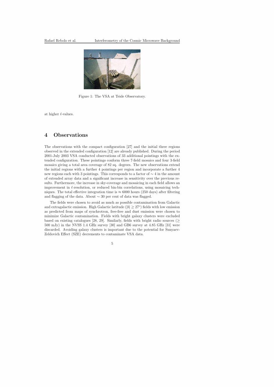
The VSA is a purpose-built 14-element radio interferometer (see Figure 1) that hasmeasured the CMB angular power spectrum between ℓ = 150 and 900 in a compactarray configuration [10] and more recently up to ℓ = 1400 in an extended arrayconfiguration [12]. It is located at Teide Observatory (Tenerife) at an altitude of2340 m. It can operate in the Ka-band (26 − 36 GHz), however, to minimize thecontribution of foregrounds to the signal recorded it was decided to operate with abandwidth of 1.5 GHz at the higher end of the band (∼ 33 GHz). Each antennaconsists of a conical corrugated horn feeding a paraboloidal mirror and is placed on a4-m×3-m tip-tilt table surrounded by a metal enclosure to supress as much as possibleground emission. The VSA can observe any sky region between declination −5 and+60. It has been used in two major modes: in the compact configuration, the mirrorswere 143-mm in diameter giving a primary beam of 4.6 FWHM; in the extended one,the 322-mm diameter apertures allow longer baselines and therefore higher resolutionsto be obtained, with a primary beam of 2 FWHM. This configuration has a totalof 91 baselines with lengths ranging from 0.6 m to 2.5 m, although the maximumpossible baseline length, set by the size of the main tip-tilt table, is ∼ 4 m. Thesynthesized beam of a typical VSA field has FWHM ∼ 11 arcmin over the primarybeam.
Combining all 91 baselines the VSA point source sensitivity is ∼ 6 Jy s1/2. Thiscorresponds to a temperature sensitivity, over a synthesized beam area (Ωsynth ≈1× 10⁻⁵ sr) of ∼ 15 mK s1/2. The exact value depends on the beam area and on theu, v coverage which in turns depends on the declination and the flagging/filtering ofthe visibility data.
An important feature of the VSA is the ability to subtract radio sources whichcontaminate CMB data with a dedicated facility. Combined with map-making capa-bilities, this makes the VSA ideal for making precise CMB measurements, particularly
4
Rafael Rebolo et al. Interferometry of the Cosmic Microwave Background
Figure 1: The VSA at Teide Observatory.
at higher ℓ-values.
4 Observations
The observations with the compact configuration [27] and the initial three regionsobserved in the extended configuration [12] are already published. During the period2001-July 2003 VSA conducted observations of 33 additional pointings with the ex-tended configuration. These pointings conform three 7-field mosaics and four 3-fieldmosaics giving a total area coverage of 82 sq. degrees. The new observations extendthe initial regions with a further 4 pointings per region and incorporate a further 4new regions each with 3 pointings. This corresponds to a factor of ∼ 4 in the amountof extended array data and a significant increase in sensitivity over the previous re-sults. Furthermore, the increase in sky-coverage and mosaicing in each field allows animprovement in ℓ-resolution, or reduced bin-bin correlations, using mosaicing tech-niques. The total effective integration time is ≈ 6000 hours (250 days) after filteringand flagging of the data. About ∼ 30 per cent of data was flagged.
The fields were chosen to avoid as much as possible contamination from Galacticand extragalactic emission. High Galactic latitude (|b| ≥ 27) fields with low emissionas predicted from maps of synchrotron, free-free and dust emission were chosen tominimize Galactic contamination. Fields with bright galaxy clusters were excludedbased on existing catalogues [28, 29]. Similarly, fields with bright radio sources (≥500 mJy) in the NVSS 1.4 GHz survey [30] and GB6 survey at 4.85 GHz [31] werediscarded. Avoiding galaxy clusters is important due to the potential for Sunyaev-Zeldovich Effect (SZE) decrements to contaminate VSA data.
5

Rafael Rebolo et al. Interferometry of the Cosmic Microwave Background
5 Data reduction and calibration
The VSA data reduction and calibration procedures are described for the compactand extended configuration in several papers [27, 12]. In [17] full details are givenabout the reduction of the new extended data. Fourier filtering is used to remove themajority of local undesired signals. The filtering removes typically 10 − 20 per centof the data. The same fringe-rate filtering technique is also applied to the Sun andMoon. Data are filtered if the Sun and Moon are within 27 and 18 respectively,while if the Sun or Moon are within 9 of the field centre then the entire observationis flagged. No residual Sun or Moon contamination was detected after stacking thedata typically integrated over 50− 100 days. The data are then further smoothed bya factor of 4 to give 64 sec samples and a correction is applied for the atmosphericcontribution to the system noise.
Noise figures vary significantly between baselines, so the final step for each ob-servation is the re-weighting of the data based on the r.m.s. noise of each baseline.This is essential to achieve the optimum overall noise level. The data are then stackedtogether either in hour angle or in the u, v plane. The final data for each field contains∼ 106 visibilities, each of 64 sec integration, which are used directly to make maps.For power spectrum estimation, the data are binned in the u, v plane to reduce thenumber of data points. Each visibility has an associated weight calculated by thereduction pipeline.
The first important step in the calibration of the VSA data is to obtain a precisegeometric description of the instrument, i.e. to know the positions for each hornewith a precission better than 1/10 the wavelength of observation. This also requiresthe calculation of corrections for amplitudes, phases and the observing frequency. Amaximum-likelihood method [32] is used to solve simultaneously all these parameters.Typically, data from an intense radiosource (like Tau-A) are collected for this purpose.The results are checked via observations of other bright radio sources. Amplitude andphase corrections are usually calculated from a single calibrator for each of the 91baselines. An unresolved, non-variable bright radio source allows the measured fringesto be corrected for amplitude and phase.
The absolute flux calibration of VSA is made using observations of Jupiter. Inthe first years of observations we assumed for this planet a brightness temperatureTJup = 152±5 K (3 per cent accuracy in temperature) at 32 GHz [33]. However, datafrom WMAP gives a more precise determination of the brightness temperature forJupiter of TJup = 146.6± 2.0 K at 33.0 GHz [34] corresponding to an accuracy of 1.5per cent in temperature terms, or equivalently 3 per cent in the CMB power spectrum(∆T 2). We have adopted this WMAP temperature for Jupiter in the calibration ofthe new extended array data, and consistently scaled our earlier measurements of thepower spectrum.
A number of data checks are systematically applied to the data (stacking data in
6

Rafael Rebolo et al. Interferometry of the Cosmic Microwave Background
various ways, splitting in different subsets, non-Gaussian tests to search for residualsystematics, etc.), but more importantly, a parallel independent reduction for themajority of the data is performed by the three institutions in the VSA collaboration.The comparison of this independent data reduction showed good agreement for bothmaps and power spectrum measurements.
6 Foregrounds
Radiosources in the fields observed by VSA are first surveyed with the Ryle Telescopeat 15 GHz to a limiting flux density of ∼ 10 mJy [35]. Then these sources are followedwith the Source Subtractor (SS), a two-element interferometer located next to theVSA main array operating at the same frequency. It consists of two 3.7 m disheswith a baseline of 9 m providing a resolution of ∼ 3 arcmin. The observations areconducted simultaneously with VSA, so each source is observed many times duringthe period of time dedicated to each VSA field. The SS data are calibrated using theflux of the planetary nebula NGC7027, assuming a flux density of (5.45 ± 0.20) Jyat 32.0 GHz and a flat spectral index α = 0.1 ± 0.1 [33]. The SS flux densities ofthe sources in the VSA fields are subtracted from the visibility data down to a levelof 20 mJy (∼ 8 µK over the synthesized beam area. The complete source survey ispresented by [70]. These source counts are also used to re-scale the 30 GHz differentialsource count model [36] and to make an estimate of the contribution from faint sourcesbelow the source subtraction limit of 20 mJy. The residual source power spectrum(∼ 210 µK2 at ℓ = 1000) is subtracted from the VSA band-power estimates as anuncorrelated statistical correction.
6.1 Galactic foregrounds
At the frequency and high angular resolution of the VSA observations it is not ex-pected a significant contribution of the diffuse Galactic foregrounds: synchrotronemission, free-free emission from ionized gas and vibrational dust emission. Thepower spectrum of these well known foregrounds decreases with increasing ℓ [37] andthe VSA fields have been selected in regions of high galactic latitude in order tominimize these potential contaminants. Estimates for these foregrounds in the VSAfields have been obtained using three template maps: the 408 MHz all-sky map forsynchrotron [38], the Hα data from the Wisconsin H-Alpha Mapper (WHAM, [39])for free-free emission and the 100 µm map [40] for dust-correlated emission. Sim-ilar considerations as in previous work [27] lead to synchrotron and free-free r.m.s.power values for the VSA extended fields of less than (10 µK2) compared to the CMBfluctuations ( >
∼ 1000 µK2).
In addition, we have to consider a more controversial foreground, the so called
7
Rafael Rebolo et al. Interferometry of the Cosmic Microwave Background
“foreground X” [41], which appears to be correlated with far infrared dust emission.The characteristics of this foreground have not been fully established yet. Somemodels [42] predict that spinning dust particles may be the carrier with maximumemission in the range 20-30 GHz. For the dust-correlated component, we smoothedthe [40] 100 µm map to 22 arcmin (ℓ ∼ 1000) and assumed a nominal couplingcoefficient between brightness temperature at 33 GHz and the 100 µm intensity ofTb/I100 = 10 µK/(MJy sr−1). This is a nominal value averaged for the high latitudesky. The r.m.s. power fluctuations estimates for the VSA fields range between 1 and90 µK2 at ℓ = 1000, typically <
∼ 10 µK2 while the CMB fluctuations are ∆T 2rms ∼
1000 µK2 thus, for most of the VSA regions, the Galactic emission is essentiallynegligible.
6.2 SZ clusters
The VSA fields are selected to avoid known galaxy clusters and minimize any contri-bution to the CMB temperature from inverse Compton scattering of hot electrons inthe intracluster medium, the Sunyaev-Zeldovich (SZ) effect [43, 3]. At the frequencyof VSA obsrvations, the SZ effect, produces temperature decrements in the line ofsight of the galaxy clusters. The confusion noise produced by a Poisson distributionof unknown high redshift clusters has been estimated using available models [44]. Ifwe adopt σ8 = 0.9, we obtain a contribution of ≈ 1 mJy beam−1, approximately sixtimes lower than the noise level in typical VSA maps.
7 Results
7.1 Maps
The maps are produced using a maximum entropy method (MEM) [45]. The binnedvisibility data used for deriving the power spectrum are also the starting point formap making. First, the Fourier modes in the u, v-plane are reconstructed, then theseare Fourier transformed to obtain the maps. The MEM algorithm assumed a flat skyas prior. The signal-to-noise ratio of the maps is in the range SNR∼ 1−3, the changebeing primarily due to the varying integration times after flagging and filtering of thedata [17]. The sensitivity of the mosaiced maps is slightly higher than this, due tothe overlapping of the individual fields.
The VSA maps allow a comparison to be made with other CMB data. The recentWMAP data release [14] has provided 5 all-sky maps at frequencies centred at 22.8(K-band), 33 (Ka-band), 40.7 (Q-band), 60.8 (V-band) and 93.5 GHz (W-band) withresolutions ranging from 49.2 arcmin (K-band) to 12.6 arcmin (W-band). The signal-to-noise ratio of WMAP data at the VSA resolution is ∼ 1 and hence much of theCMB signal is lost in the noise. The actual noise level in the WMAP data depends on
8

Rafael Rebolo et al. Interferometry of the Cosmic Microwave Background
position due to the scanning strategy of the WMAP satellite. For the 1-year WMAPdata release, the noise is ∼ 100 − 200 µK per 12.6 arcmin pixel in the VSA regions,compared to ∼ 20 µK beam−1 in the VSA mosaiced maps.
7.2 Power spectrum
The final visibility data are binned into u, v square cells, each 9 wavelengths on aside, to oversample the data. This reduces the number of data points by a factor of>∼ 1000. Sources are subtracted using position and flux density information from theSource Subtractor. For each VSA pointing there is a final visibility file with ∼ 103
data points.
Figure 2: The CMB power spectrum as measured by the VSA by combining the datafrom all 7 VSA regions [17]. The first 3 bins are included from earlier VSA datain a compact array. The errors represent 1 σ limits. Two alternate binnings (greyand black) are displayed. Absolute calibration is accurate to 3 per cent and is notincluded in the errors.
The binned visibilities form the basic input to the maximum likelihood analysisfor the CMB power spectrum. We used the Microwave Anisotropy Dataset Compu-tational sOftWare (MADCOW) [46] which can deal with mosaiced observations andvariable bin-widths.The band powers calculated from the complete VSA data set,both the compact and extended arrays are available at the following URL:http://www.jb.man.ac.uk/research/vsa/vsa results.html.
The extended array data have little sensitivity at ℓ <∼ 300. The 3 bins at ℓ < 300
are therefore dominated by data from the compact array [10]. The error bars werecalculated from the probability likelihood functions by enclosing 68 per cent of thearea centred on ℓh, the median ℓ value for each bin. Calibration uncertainty (≈ 3per cent) is not included. Sample variance is included in the error estimates. The
9

Rafael Rebolo et al. Interferometry of the Cosmic Microwave Background
VSA power spectrum (Figure 2) clearly shows the existence of the first three acousticpeaks and the fall-off in power towards higher ℓ.
8 Cosmological implications
We first consider the standard six-parameter flat ΛCDM model, and then includeextra parameters as in the approach adopted by the WMAP team [16, 47, 48]. In thecase where we do not impose external priors on the CMB data (WMAP+VSA), wefind that there is significant evidence (> 2σ) for negative running; something whichis not implied by the WMAP data alone. The significance of this result is sensitiveto the inclusion of external priors, the relative calibration of WMAP and VSA, andpossible source/cluster contamination of the measured power spectrum. Second, weconsider a 12-parameter model fit to WMAP, WMAP+VSA and all available CMBdata beyond ℓ > 1000, illustrating the effects of external priors on the estimatedparameters.
8.1 Methodology
Cosmological model
The ΛCDM model assumes that the Universe is flat and dominated by cold darkmatter (CDM), baryons and a cosmological constant, Λ. The densities of thesecomponents relative to critical are denoted Ωdm, Ωb and ΩΛ respectively and wedefine Ωm = Ωdm + Ωb to be the overall matter density (CDM and baryons) inthe same units. The expansion rate is quantified in terms of the Hubble constantH0 = 100hkmsec−1 Mpc−1 and we allow for instantaneous reionization at some epochzre(< 30) which can also be quantified in terms of an optical depth τ . The so-called physical densities of the CDM and baryons are defined as ωdm = Ωdmh2 andωb = Ωbh
2. We will consider only adiabatic models and parameterize the initialfluctuation spectrum of this model by
P (k) = AS
(
k
kc
)nS
, (7)
where kc = 0.05Mpc−1 is the arbitrarily chosen pivot point of the spectrum, nS is thespectral index and AS is the scalar power spectrum normalization.
We will also consider a model with a running spectral index,
P (k) = AS
(
k
kc
)nS+ 1
2nrun log(k/kc)
, (8)
10

Rafael Rebolo et al. Interferometry of the Cosmic Microwave Background
so that the overall spectral index of fluctuations is a function of scale, nS(k), givenby
nS(k) =d(log P )
d(log k)== nS + nrun log
(
k
kc
)
, (9)
where nrun is known as the running of the spectral index. For slow roll inflation to bewell defined, one requires that |nrun| ≪ |1−nS|/2 [49]. Under certain choices of priorswe find that there is some evidence that this inequality is violated by the preferredfits to the data.
The other parameters which we will consider in our analyses are: fν = Ων/Ωdm,the fraction of the dark matter which is massive neutrinos; Ωk = 1 − Ωtot (Ωtot =Ωdm + Ωb + Ων + ΩΛ), the curvature in units of the critical density; w = PQ/ρQ, theequation-of-state parameter for a dark energy component modelled as a slowly rollingscalar field; nT the spectral index of tensor fluctuations specified at the pivot pointkc = 0.002 Mpc−1; R = AT/AS, the ratio of the amplitude of the scalar fluctuations,AS, evaluated at kc = 0.05 Mpc−1, and that of the tensor fluctuations evaluated atkc = 0.002 Mpc−1. In addition to these parameters, for which we fit, we will alsocomment on various derived quantities: t0, the age of the universe; σ8, the amplitudeof density fluctuations in the spheres of 8h−1 Mpc.
8.2 CMB data
Four different combinations of CMB data have been considered.
• The first data set, denoted COBE+VSA contains the VSA data as describedin the previous sections [17] combined with the COBE data [4, 50].
• The second data set, denoted WMAP contains only the WMAP temperature(TT) data [15] and temperature-polarization cross-correlation (TE) data [51].
• The third data set contains WMAP data and the new VSA data and is referredto as WMAP+VSA. This allows to illustrate the relevance of measurementsof the power spectrum on small angular scales.
• Finally, we combine the previous two with all important CMB experimentsproviding measurements in the region of the second peak of the spectrum andbeyond, namely CBI, ACBAR, Boomerang, Maxima, DASI [11, 13, 7, 52, 8].This last data set is hereafter referred to as AllCMB.
External priors
In addition to the CMB data sets described above, we consider the effects of othercosmological data, not only to break the degeneracies, but also to see how the mea-
11

Rafael Rebolo et al. Interferometry of the Cosmic Microwave Background
sured CMB power spectrum fits in the wider cosmological context. The externalpriors used are:
• The constraint on the expansion rate of the Universe from the Hubble SpaceTelescope (HST) Key project value of H0 = 72 ± 8 kmsec−1 Mpc−1 [53]. Theerror-bar includes both statistical and systematic uncertainty.
• Constraints on large scale structure from the 2dF Galaxy Redshift Survey [54,55, 56], which provides measurements on scales 0.02 < k/(hMpc−1) < 0.15.
• Constraints from Type Ia Supernovae (SNeIa) [57, 58].
• Constraints from the gas fraction (fgas) in dynamically relaxed clusters of galax-ies [59] and from the observed local X-ray luminosity function (XLF) of galaxyclusters [60].
• Constraints from cosmic shear (CS) measurements [61].
Parameter estimation
The parameter estimation has been performed using the cosmomc software package[62]. The calculations were performed on LAM clusters with a total of 42 CPUs at theIAC in La Laguna, Tenerife and the COSMOS supercomputer facility at the Uni-versity of Cambridge. The cosmomc software uses the Markov Chain Monte Carlo(MCMC) algorithm to explore the hypercube of parameters on which we impose flatpriors. These priors are listed in Table 8.2. Additionally, the software automaticallyimposes the physical prior ΩΛ > 0, which can significantly affect the marginalizedprobability distributions (see [63] for further discussion).
8.3 Flat ΛCDM models
Standard six-parameter model
We begin our discussion in the context of the standard flat ΛCDM model with sixfree parameters (ωb, ωdm, h, nS, AS, τ) with no external priors.
The constraints derived for the parameters are tabulated in Table 8.3. The valuesfor WMAP alone can be compared with those in [16]. Noting that they presentωm = Ωmh2, instead of ωdm, there are only minor discrepancies in the central values,although some of the limits appear to be somewhat larger. The preferred valueof the redshift of reionization is zre = 17+8
−6. The inclusion of the high-resolutiondata from the VSA modifies the limits on each of the parameters and these aremost significant for nS, whose best fitting value reduces from 1.00 to 0.97. Theresult for nS will be central to our subsequent discussion of the primordial power
12

Rafael Rebolo et al. Interferometry of the Cosmic Microwave Background
Basic Parameter Priorωb (0.005,0.10)ωdm (0.01, 0.99)h (0.4,1.0)nS, n1, n2 (0.5,1.5)zre (4,30)1010AS (10,100)nrun (−0.15,0.15)AX/(µK)2 (−500,500)fν (0,0.2)Ωk (−0.25,0.25)w (−1.5,0)R (0,2)nT (−1.5,3)
Table 1: Priors used on each cosmological parameter when it is allowed to vary. Thenotation (a, b) for parameter x denotes a top-hat prior in the range a ≤ x ≤ b.
Parameter COBE+VSA WMAP WMAP+VSA
ωb 0.0328+0.0073−0.0071 0.0240+0.0027
−0.0016 0.0234+0.0019−0.0014
ωdm 0.125+0.031−0.027 0.117+0.018
−0.018 0.111+0.014−0.016
h 0.77+0.15−0.17 0.73+0.10
−0.06 0.73+0.09−0.05
nS 1.05+0.12−0.08 1.00+0.09
−0.04 0.97+0.06−0.03
1010AS 25+11−6 27+9
−5 23+7−3
τ Unconstrained 0.18+0.16−0.08 0.14+0.14
−0.07
Table 2: Parameter estimates and 68% confidence limits for the standard six-parameter flat ΛCDM model.
13

Rafael Rebolo et al. Interferometry of the Cosmic Microwave Background
CMB External nS nrun
COBE+VSA None 0.93+0.13−0.12 −0.081+0.049
−0.049
WMAP None 0.94+0.07−0.06 −0.060+0.037
−0.036
WMAP+VSA None 0.96+0.07−0.07 −0.069+0.032
−0.032
COBE+VSA HST 0.92+0.11−0.12 −0.081+0.048
−0.048
WMAP HST 0.95+0.06−0.07 −0.060+0.037
−0.037
WMAP+VSA HST 0.93+0.06−0.05 −0.069+0.036
−0.036
COBE+VSA 2dF 1.00+0.12−0.13 −0.044+0.058
−0.061
WMAP 2dF 0.95+0.05−0.06 −0.038+0.025
−0.037
WMAP+VSA 2dF 0.93+0.05−0.05 −0.049+0.035
−0.034
Table 3: Limits on nS and nrun in the flat ΛCDM model with a running spectral indexfor different CMB data sets and external priors.
spectrum. The results from WMAP+VSA are very similar to those presented in[16] for WMAP+ACBAR+CBI. We also find a larger value for ωb than suggested byWMAP, WMAP+VSA and standard Big Bang Nucleosynthesis, ωb = 0.020± 0.002,[64].
Running spectral index models
In the previous section we saw that the inclusion of the VSA data to that of WMAPshifts the derived limits on the spectral index. Standard, slow-roll models of inflationpredict that the spectral index will be a function of scale, albeit at a very low level,and it seems a sensible parameter to allow as the first beyond the standard model. Theanalysis of [16, 48] provided evidence for a non-zero value of nrun(= −0.031+0.016
−0.017) whenusing CMB data from WMAP, ACBAR and CBI, along with large-scale structure data
14

Rafael Rebolo et al. Interferometry of the Cosmic Microwave Background
from the 2dF galaxy redshift survey and the Lyman-α forest.
We will start our discussion by considering the same model as in the previoussection with no external priors, but with nrun allowed to vary. The derived limitson nS and nrun are presented in the first three rows of Table 8.3 for COBE+VSA,WMAP and WMAP+VSA. The derived limits on ωb, ωdm and h are not changedappreciably and the other parameters, AS and τ (or zre) are strongly degenerate andzre will feature in our discussion below.
The values of nS and nrun are not particularly well constrained by COBE+VSA,but it is worth noting that even in this case there is a definite preference for a valueof nrun < 0. The results have been included for completeness and provide a usefulcross-check. The results for WMAP are somewhat different to those presented in[16]. In particular we find that nrun = −0.060+0.037
−0.036, a 1.6σ preference for nrun < 0,as opposed to nrun = −0.047± 0.04 from Spergel et al. [16]. The significance of thisresult is improved to 2.2σ by the inclusion of the high resolution data from the VSA.We remark that this result comes from CMB data alone.
We have tested the sensitivity of this apparently result to the inclusion of externalpriors from the HST and 2dF galaxy redshift survey, and the results are also presentedin Table 8.3. We see that the effect of the HST prior is to relax marginally theconstraint on nrun, although there is a significant change in the derived limit on nS.We note that the results for WMAP alone are very similar with and without the HSTprior. The inclusion of 2dF does significantly affect our results. Using just WMAPwe find that there is only a marginal preference for nrun < 0 and the inclusion of VSAonly yields a 1.4σ result. We note that this is a shift in the derived value and theerror bars do not change significantly.
We have also considered the effects of including other CMB information from thetwo other high resolution experiments ACBAR and CBI. We find that the inclusionof their results does not appear to be as significant as the VSA in preferring a valueof nrun < 0 and that the result of considering WMAP+ACBAR+CBI+VSA is verysimilar to just WMAP+VSA. We note that the ACBAR and CBI experiments quotelarge global calibration uncertainties (20% and 10% in power), which we believe is atleast as responsible for this result as their errors on the individual power spectrumband powers.
Neutrino fraction
As a final extension to our flat ΛCDM model, it is of interest to include the fractionfν of dark matter in the form of neutrinos. Evidence for a neutrino oscillation, andhence for the existence of massive neutrinos, has been found by solar neutrino andatmospheric neutrino experiments [65, 66, 67, 68]. Further evidence for a non-zerovalue of the neutrino mass has recently been claimed from cosmological data [69].
In addition to obtaining constraints on fν, the inclusion of this parameter will
15

Rafael Rebolo et al. Interferometry of the Cosmic Microwave Background
inevitably lead to some broadening of the marginalized distributions for the otherparameters. Of particular interest is whether the constraints on the running spectralindex derived above are robust to the inclusion of fν . We therefore include fν , withthe top-hat prior given in Table 8.2, into the running spectral index model. In theanalysis of this model, we include the 2dF external prior, since current CMB aloneprovide only a weak constraint on fν .
We find that the 95% upper limit provided by the COBE+VSA data set, fν <0.132, is only marginally larger than that obtained using WMAP data, fν < 0.090.The combination WMAP+VSA gives similar limits to WMAP, namely fν < 0.087,which corresponds to neutrino mass of mν < 0.32eV when the neutrino masses aredegenerate.
For the parameters nS and nrun, the marginalized distributions have indeed beenshifted and broadened by the inclusion of fν although the effects are not very strong.In particular, we note that our earlier finding of a preference for a non-zero value ofnrun has been weakened somewhat. A non-zero nrun is still preferred, but at reducedsignificance. For the WMAP+VSA data set, we obtain nS = 0.94+0.06
−0.06 and nrun =−0.041+0.037
−0.036 with 68% confidence limits.
In the above analysis we used only 2dF as an external prior. It is of interest toinvestigate the effect of including different combinations of the additional externalpriors listed in Table 8.2. The effect of these additional priors has been calculatedby importance sampling our previous results. We also investigate the effect of in-cluding all recent CMB data into our analysis. In Figure 3, we plot confidencelimits on all the model parameters for each of our four CMB data sets, each ofwhich, in turn, includes four different combinations of external priors: 2dF, 2dF+fgas,2dF+fgas+XLF, 2df+HST and 2dF+CS. The points indicate the median of the cor-responding marginalized distribution, and the error bars show the 68% central confi-dence limit. If the distribution peaks at zero, the point is placed on the axis and the95% upper limit is shown.
We see that the inclusion of the fgas and XLF external priors significantly reducesthe error bars on all parameters. The most profound effect is obtained from the XLFprior for the parameters fν , σ8 and zre, as might be expected from [69]. Indeed, itis only with the inclusion of the XLF prior that a non-zero value of fν is preferredand only then at limited significance. For each of the CMB data set combinations,the best-fitting value in this case is fν ≈ 0.05, which corresponds to neutrino mass ofmν ≈ 0.18eV when the neutrino masses are degenerate, with a zero value excluded ataround 96% confidence. For σ8 the inclusion of the XLF prior significantly reducesthe best-fit value and the error bars for all CMB data set combinations. A similar,but less pronounced, effect is seen for zre.
16

Rafael Rebolo et al. Interferometry of the Cosmic Microwave Background
WMAP WMAP+VSA AllCMB
Ωbh2 0.025+0.003
−0.003 0.024+0.003−0.002 0.023+0.002
−0.002
Ωdmh2 0.108+0.022−0.021 0.111+0.021
−0.019 0.113+0.017−0.017
h 0.66+0.07−0.06 0.66+0.06
−0.06 0.65+0.07−0.07
zre 18+7−7 19+7
−7 17+7−8
Ωk −0.02+0.03−0.03 −0.01+0.03
−0.03 −0.02+0.03−0.03
fν < 0.093 < 0.083 < 0.083
w −1.00+0.24−0.27 −0.99+0.24
−0.27 −1.06+0.24−0.25
nS 1.04+0.12−0.11 0.99+0.09
−0.09 0.96+0.07−0.07
nT 0.26+0.53−0.60 0.13+0.49
−0.51 0.12+0.48−0.51
nrun −0.02+0.07−0.05 −0.04+0.05
−0.04 −0.04+0.04−0.05
1010AS 27+8−5 26+9
−5 25+6−5
R < 0.78 < 0.77 < 0.68
ΩΛ 0.71+0.07−0.09 0.70+0.06
−0.08 0.69+0.07−0.09
t0 14.1+1.4−1.1 14.1+1.3
−1.2 14.4+1.4−1.3
Ωm 0.31+0.09−0.07 0.31+0.08
−0.06 0.33+0.10−0.07
σ8 0.76+0.14−0.14 0.77+0.13
−0.13 0.76+0.11−0.12
τ 0.20+0.13−0.11 0.20+0.15
−0.10 0.17+0.12−0.10
Table 4: Parameter estimates and 68% confidence intervals for various cosmologicalparameters. For fν and R, the 95% upper limits are quoted.
17

Rafael Rebolo et al. Interferometry of the Cosmic Microwave Background
Figure 3: Estimates for cosmological parameters in the flat ΛCDM running spectralindex model, extended to include fν . Four CMB data sets are considered and, foreach data set, four determinations are plotted, corresponding to different combina-tions of external priors. From left to right the external priors are: 2dF; 2dF+fgas;2dF+fgas+XLF; 2dF+HST and 2dF+CS. The points indicate the median of the cor-responding marginal distributions. The error bars denote 68% confidence limits. If adistribution peaks at zero then the 95% upper limit is shown. The horizontal dashedlines plotted in some of the panels indicate BBN values for Ωbh
2, the value of hgiven by the HST key project, the Harrison-Zeldovich value of the spectral index offluctuations and a zero value for the running index.
18

Rafael Rebolo et al. Interferometry of the Cosmic Microwave Background
8.4 General ΛCDM model
Thus far we have considered only a limited range of flat ΛCDM models. In principle,one should properly include all the relevant unknowns into the analysis in order toobtain conservative confidence limits. In this section, we consider a more generalΛCDM model. In addition to including fν and nrun, the standard six-parameter flatΛCDM model is further extended by including Ωk, w, R = AT/AS and nT. Thisgives 12 variable parameters in total, for which we adopt the top-hat priors listed inTable 8.2.
For this model, we consider the three CMB data sets WMAP, WMAP+VSA andAllCMB. In addition, we now use both 2dF and SNeIa as our basic external priors,which are required in order to set constraints on our 12-dimensional cosmologicalparameter space. The corresponding confidence limits on the parameter values aregiven in Table 8.3.
For Ωbh2 we see a clear trend towards a lower preferred value (closer to the BBN
estimate) as one adds first VSA data and then all remaining CMB data sets. Thiseffect is accompanied by a gradual upwards trend in the preferred Ωdmh2 value. Theother parameters exhibiting such trends are nS and nrun. As more CMB data areincluded, the preferred value of nS moves slightly below unity, although this value is byno means excluded. Perhaps more importantly, the upper limit on nS is significantlyreduced as more CMB data are added. An analogous effect is observed for nrun, forwhich the addition of VSA data significantly reduces the tail of the distribution forpositive values of nrun.
We see that the inclusion of the fgas and XLF external priors has the greatesteffect on the confidence limits, and that this is most pronounced for the XLF priorand the parameters fν , σ8 and zre. It is reassuring, however, that the derived limits onfν for the general model are very similar to those obtained assuming the simpler flatmodel. We again find fν ≈ 0.05, with a zero-value excluded at about 92% confidencewhich is slightly lower than for the flat case. The effect of the XLF prior on σ8 andzre in the general model is also similar to that observed in the simpler flat case.
9 Conclusions
We have used recent data from the Very Small Array, together with other CMBdatasets and external priors, to set constraints on cosmological parameters. We haveconsidered both flat and non-flat ΛCDM models and the results are consistent.
Within the flat ΛCDM model, we find that the inclusion of VSA data suggeststhat the initial fluctuation spectrum that is not described by a single power-law. Thenegative running, which reduces the amount of power on small scales and hence theamount of structure at early times, leads to predictions for the epoch of reionizationat odds with the best fit to the CMB data. We shall caution that this result may
19

Rafael Rebolo et al. Interferometry of the Cosmic Microwave Background
be affected by the absolute calibration uncertainty of the VSA power spectrum andthe residual point source correction due to sources below out subtraction limit of20mJy. It is possible that an imperfect subtraction, either an over-estimate or anunder-estimate, could lead to inaccuracies in the derived limits on the cosmologicalparameters, in particular on nS and nrun.
For the general 12-parameter ΛCDM model, we find that our marginalized distri-butions for nS and nrun are broadened, as one would expect. Nevertheless, even in thiscase, the addition of VSA data significantly reduces tails of the distributions for nS
greater than unity and for positive nrun, as compared with using WMAP as the onlyCMB data set. Indeed, these effects are reinforced by the use of the AllCMB dataset. The inclusion of additional CMB data beyond WMAP also leads to a noticeablereduction in the preferred value of ωb and a corresponding increase in ωdm.
To summarize, we find that there is evidence for nrun < 0 in a limited classof models, but within the general ΛCDM model with 12 parameters the evidence ismuch weaker. Standard models of inflation are generally incompatible with such largenegative values of nrun, but the data appears to point in that direction, although nottotally conclusively. The inclusion of an external prior from 2dF appears to weakenthe result by fixing Ωm ≈ 0.3 in conjunction with the CMB data. The measurement ofΩmh using the galaxy power spectrum is responsible for this shift. It is an interestingquestion as to how reliable this measurement is since a slight shift in the results, apreference for Ωmh ≈ 0.17 rather than Ωmh ≈ 0.21 would bring their preferred valueinto line with that suggested by the CMB alone and would uphold the possibilityof nrun < 0. Since none of the galaxy redshift surveys have conclusively observedthe turnover in the power spectrum on which this determination of Ωmh is based weassert that there is still room for some doubt. We set an upper limit on the mass ofeach of the three neutrino flavours of mν < 0.32eV (95 C.L.). We have shown thatmeasurements of the CMB power spectrum beyond ℓ = 1000 can have an impacton the estimation of cosmological parameters and that future measurements in thisregion by the VSA, the PLANCK satellite and others will enable us in the future tomake more definitive statements.
Acknowledgements: We thank the staff of Jodrell Bank Observatory, Mullard RadioAstronomy Observatory and IAC for assistance in the day-to-day operation of theVSA. We thank PPARC and the IAC for funding and supporting the VSA project.Partial financial support was provided by Spanish Ministry of Science and Technologyproject AYA2001-1657.
References
[1] Fixen, D. J., Cheng, E. S., Gales, J. M., Mather, J. C., Shafer, R. A., Wright,E. L. 1996, ApJ, 473, 576
20

Rafael Rebolo et al. Interferometry of the Cosmic Microwave Background
[2] Peebles, P.J.E. and Yu, J. T. 1970, ApJ, 162, 815[3] Sunyeav, R. A., Zeldovich, Y. B. 1970, ApJSS, 7, 3[4] Smoot G. F. et al. 1992, ApJ, 396, L1[5] de Bernardis, P. et al. 2000, Nature, 404, 955[6] Lee A. T. et al. 2001, ApJ, 561, L1[7] Netterfield C. B. et al. 2002, ApJ, 571, 604[8] Halverson N. W. et al. 2002, ApJ, 568, 38[9] Benoıt A. et al. 2003, A&A, 399, L19
[10] Scott P. F. et al. 2003, MNRAS, 341, 1076[11] Pearson T. J. et al. 2003, ApJ, 591, 556[12] Grainge K.J.B. et al. 2003, MNRAS, 341, L23[13] Kuo C. L. et al. 2004, ApJ, 600, 32[14] Bennett C. L. et al. 2003a, ApJSS, 148, 1[15] Hinshaw, G. et al. 2003a, ApJSS, 148, 135[16] Spergel D. N. et al. 2003, ApJSS, 148, 175[17] Dickinson C. et al. 2004, MNRAS, submitted[18] White, M., Carlstrom, J. E., Dragovan, M., and Holzapfel, W. L. 1999, ApJ,
514, 12[19] Rebolo R. 2002, Space Sci. Rev., 100, 15[20] White, M., Srednicki, M. 1995, ApJ, 443, 6[21] Webster, A. 1994, MNRAS, 268, 299[22] Church, S. E. 1995, MNRAS, 272, 551[23] Dicker, S. R., Melhuish, S. J., Davies, R. D., Gutierrez, C. M., Rebolo, R.,
Harrison, D. L., Davis, R. J., Wilkinson, A., Hoyland, R. J., Watson, R.A. 1999,MNRAS, 309, 750
[24] Harrison, D. L., Rubino-Martın, J. A., Melhuish, S. J., Watson, R.A., Davies,R.D., Rebolo, R., Davis, R. J., Gutierrez, C. M., Macıas-Perez 2000, MNRAS,316, L24
[25] Padin et al. 2001, ApJ, 549, L1[26] Watson R. A. et al. 2003, MNRAS, 341, 1057[27] Taylor A. C. et al. 2003, MNRAS, 341, 1066[28] Ebeling, H., Edge, A. C., Bohringer, H., Allen, S. W., Crawford, C. S., Fabian,
A. C., Voges, W., Huchra, J. P. 1998, MNRAS, 301, 881[29] Abell G. O. 1958, ApJSS, 3, 211[30] Condon, J. J., Cotton, W. D., Greisen, E. W., Yin, Q. F., Perley, R. A., Taylor,
G. B., Broderick, J. J. 1998, AJ, 115, 1693[31] Gregory, P. C., Scott, W. K., Douglas, K., Condon, J. J. 1996, ApJSS, 103, 427[32] Maisinger, K., Hobson, M. P., Saunders, R.D.E., Grainge, K.J.B. 2003, MNRAS,
345, 800[33] Mason, B. S., Leitch, E. M., Myers, S. T., Cartwright, J. K., Readhead, A.C.S.
1999, AJ, 118, 2908[34] Page L. et al. 2003, ApJSS, 148, 39
21

Rafael Rebolo et al. Interferometry of the Cosmic Microwave Background
[35] Waldram, E. M., Pooley, G. G., Grainge, K.J.B., Jones, M. E., Saunders, R.D.E.,Scott, P. F., Taylor, A. C. 2003, MNRAS, 342, 915
[36] Toffolatti, L., Argueso Gomez, F., de Zotti, G., Mazzei, P., Franceschini, A.,Danese, L., Burigana, C. 1998, MNRAS, 297, 117
[37] Giardino, G., Banday, A.J., Fosalba, P., Gorski, K. M., Jonas, J. L., O’Mullane,W., Tauber, J. 2001, A&A, 371, 708
[38] Haslam, C.G.T., Klein, U., Salter, C. J., Stoffel, H., Wilson, W. E., Cleary,M. N., Cooke, D. J., Thomasson, P. 1981, A&A, 100, 209
[39] Haffner, L. M., Reynolds, R. J., Tufte, S. L., Madsen, G. J., Jaehnig, K. P.,Percival, J. W. 2003, ApJSS, 149, 405
[40] Schlegel, D. J., Finkbeiner, D. P., Davis, M. 1998, ApJ, 500, 525[41] de Oliveira-Costa, A., Tegmark, M., Davies, R. D., Gutierrez, C. M., Lasenby,
A. N., Rebolo, R., Watson, R. A., ApJ, submitted (astro-ph/0312039)[42] Draine, B. T., Lazarian, A. 1998, ApJ, 494, L19[43] Zeldovich, Y. B., Sunyaev, R. A. 1969,ApJSS, 4, 301[44] Battye, R. A., Weller, J. 2003, Phys. Rev. D, 68, 083506[45] Maisinger, K., Hobson, M. P., Lasenby, A. N. 1997, MNRAS, 290, 313[46] Hobson, M. P., Maisinger, K. 2002, MNRAS, 334, 569[47] Verde L. et al. 2003, ApJSS, 148, 195[48] Peiris, H. V. et al. 2003, ApJSS, 148, 213[49] Leach, S., Liddle, A. R. 2003, astro-ph/0306305[50] Bennett, C. L. et al. 1996, ApJ, ApJ, 464, L1[51] Kogut A. et al. 2003, ApJSS, 148, 161[52] Hanany S. et al. 2002, ApJ, 545, L5[53] Freedman W. L. et al. 2001, ApJ, 553, 47[54] Colless M. et al 2001, MNRAS, 328, 1039[55] Percival W. J. et al. 2001, MNRAS, 327, 1297[56] Percival W. J. et al. 2002, MNRAS, 337, 1068[57] Perlmutter S. et al. 1999, ApJ, 517, 565[58] Reiss A. et al. 1998, AJ, 116, 1009[59] Allen, S., Schmidt, R. W., Fabian, A. C. 2002, MNRAS, 334, L11[60] Allen, S., Schmidt, R. W., Fabian, A. C., Ebeling, H. 2003a, MNRAS, 342, 287[61] Hoekstra, H., Yee, H.K.C., Gladders, M. D. 2002, ApJ, 577, 595[62] Lewis, A. L., Bridle S. L. 2002, PRD, 66, 103511[63] Slosar, A. et al. 2003, MNRAS, 341, L29[64] Burles, S., Nollett, K. M., Turner, M. S. 2001,ApJ, 552, L1[65] Fukuda Y. et al. 1998, Phys. Rev. Lett., 81, 1562[66] Fukuda Y. et al. 2002, Phys. Lett. B, 539, 179[67] Allison W.W.M. et al. 1999, Phys. Lett. B, 449, 137[68] Ambrosio M. et al 2000, Phys. Lett. B, 478, 5[69] Allen, S. W., Schmidt, R. W., Bridle, S. L. 2003b, MNRAS, 346, 596[70] Cleary, K. 2003, Ph.D thesis, University of Manchester
22

WHITE DWARFS AND THE AGE OF THE
UNIVERSE
JORDI ISERNInstitut d’Estudis Espacials de Catalunya, E-08034 Barcelona, SPAINInstitut de Ciencies de l’Espai (Consejo Superior de Investigaciones Cientıficas),E-08034 Barcelona, SPAINENRIQUE GARCIA–BERROInstitut d’Estudis Espacials de Catalunya, E-08034 Barcelona, SPAINDepartament de Fısica Aplicada, Escola Politecnica Superior de Castelldefels,Universitat Politecnica de Catalunya, E-08860 Castelldefels, SPAIN
Abstract: White dwarfs are the final remnants of low and intermediate massstars. Their evolution is essentially a cooling process that lasts for ∼ 10 Gyr andallows to obtain information about the age of the Galaxy as well as about the paststellar formation rate in the solar neighborhood. One of the most important appli-cations is to pose a severe constrain to the age of the Universe. For this reason itis important to identify all the relevant sources of energy as well as the mechanismsthat control its flow to the space. In this paper we describe the state of the art of thewhite dwarf cooling theory and we discuss the uncertainties still remaining.
1 Introduction
The test of self-consistency that all the cosmological models have to fullfill is that theUniverse cannot by younger than anyone of the objects it contains. For this reason ahuge effort has been invested to identify and determine the age of the oldest objects inthe Universe: globular clusters and long-lived stars. In this contribution we examinethe role that white dwarfs can play in this affair.
White dwarfs represent the last evolutionary stage of stars with masses smallerthan 10 ± 2 M⊙, with the upper mass limit not yet well known. Most of them arecomposed of carbon and oxygen, but white dwarfs with masses smaller than 0.4 M⊙
are made of helium, while those more massive than ∼ 1.05 M⊙ are made of oxygenand neon. The exact composition of the carbon-oxygen cores critically depends on theevolution during the previous asymptotic giant branch phase, and more specificallyon the competition between the 12C(α, γ)16O reaction and the triple-α reaction, onthe details of the stellar evolutionary codes and on the choice of several other nuclear
23

Jordi Isern and Enrique Garcıa-Berro White Dwarfs
cross sections. In a typical case, a white dwarf of 0.58 M⊙, the total amount of oxygenrepresents the 62% of the total mass while its concentration in the central layers ofthe white dwarf can be as high as 85%.
In all cases, the core is surrounded by a thin layer of pure helium with a mass in therange of 10−2 to 10−4 M⊙. This layer is, in turn, surrounded by an even thinner layerof hydrogen with mass lying in the range of 10−4 to 10−15 M⊙. This layer is missing in25% of the cases. From the phenomenological point of view, white dwarfs containinghydrogen are classified as DA while the remaining ones (the non-DA) are classifiedas DO, DB, DQ, DZ and DC, depending on their spectral features, and constitutea sequence of decreasing temperatures. The origin of these spectral differences andthe relationship among them is not yet elucidated although it is related to the initialconditions imposed by the evolution of AGB stars, the diffusion induced by gravity,thermal diffusion, radiative levitation, convection at the H-He and He-core interfaces,proton burning, stellar winds and mass accretion from the interstellar medium.
The structure of white dwarfs is sustained by the pressure of degenerate electronsand these stars cannot obtain energy from thermonuclear reactions. Therefore, theirevolution can be described just as a simple cooling process [1] in which the internaldegenerate core acts as a reservoir of energy and the outer non-degenerate layerscontrol the energy outflow. If it is assumed that the core is isothermal, which isjustified by the high conductivity of degenerate electrons, and that the envelope isthin, then
L ≈ −dUth
dt= −cVMWD
dTc
dt(1)
where Uth is the thermal content, cV is the average specific heat, Tc is the temperatureof the (isothermal) core and all the remaining symbols have their usual meaning. Tosolve this equation it is necessary to provide a relationship among the luminosity andthe temperature of the core:
L
MWD= f(Tc) (2)
A simple calculation indicates that the lifetime of these stars is very long, ∼ 10Gyr, and thus they retain important information about the past history of the Galaxy.In particular, it is possible to obtain the stellar formation rate and the age of thedifferent galactic components: disk, halo and globular clusters.
2 The evolution of the envelope
As it has been mentioned earlier, the envelope of white dwarf stars is a very thin layer(Me < 10−2 M⊙), partially degenerate, partially or totally ionized and sometimes
24

Jordi Isern and Enrique Garcıa-Berro White Dwarfs
convective, that completely controls the emergent flux of energy. Its behavior is theresult of:
1. A non–standard initial chemical composition resulting from hydrogen and he-lium shell burning in AGB stars,
2. A very efficient gravitational settling that induces the stratification of the en-velope in almost chemically pure layers with the lightest element in the top [2],and
3. The existence of mechanisms tending to restore the homogeneity, like convectivemixing [3, 4, 5, 6], radiative levitation [7, 8], thermal diffusion [2], accretion fromthe interstellar medium [9], winds and so on.
There is now a broad opinion that the distinction among the character DA andnon–DA is inherited (i.e., it is linked to the origin of the white dwarf itself) although afraction of them can change their external aspect during the evolution [10]. Standardevolution theory predicts that typical field white dwarfs have a core mass in therange of 0.5 to 1.0 M⊙ made of a mixture of carbon and oxygen surrounded bya helium mantle of MHe ≃ 10−2MWD, surrounded itself by a hydrogen envelope ofMH ≃ 10−4MWD [3, 11, 12]. Adjusting the parameters in the AGB models it is possibleto obtain in the 25% of the cases a white dwarf totally devoid of the hydrogen layer.Since the relative number of DA/non–DA stars changes as the evolution proceeds, amechanism able to change this property must exist [10, 13].
The idea is that DA white dwarfs start as a central star of a planetary nebula.When its temperature is high enough (Teff > 40, 000 K) radiative levitation bringsmetals to the photosphere and heavy element lines appear in its spectrum. As thetemperature goes down, these elements settle down and disappear. When DAs arriveto the instability strip they pulsate as ZZ Ceti stars. Pulsational data indicates thatthe masses of the hydrogen layer are in the range between 10−8 and 10−4 M⊙ thusindicating that DAs are born with a variety of layer masses. As the DA star coolsdown, the convective region deepens and, depending on the mass, reaches the heliumlayer. When this happens, helium is dredged up and the DA white dwarf turns into anon–DA. Consequently, the ratio between the number of DAs and non–DAs decreases.Stars with a thin H layer (< 10−9 M⊙) mix at high temperatures while those havinga thick layer (∼ 10−4 M⊙) never do it.
The evolution of a non–DA star is more complex. They are born as He-richcentral stars of planetary nebulae and, as they cool down, they become first PG 1159stars and then DO stars. The trace amounts of hydrogen still present in the heliumenvelope gradually float up to the surface and when the effective temperature is ofthe order of 50,000 K the outer H layer becomes thick enough to hide the He layerand to convert the star into a DA star. When the temperature drops below 30,000 K,
25

Jordi Isern and Enrique Garcıa-Berro White Dwarfs
Figure 1: Oxygen profile of a 0.61 M⊙ white dwarf at the beginning of the thermally-pulsing AGB phase (dotted line), the same after rehomogenization by Rayleigh-Taylorinstabilities during the liquid phase (dotted-dashed line) and after total freezing (solidline).
the helium convection zone increases and hydrogen is engulfed and mixed within thehelium layer once more. The white dwarf is observed as a non–DA, more precisely asa DB. This lack of non–DA stars in the temperature range of 30,000 to 45,000 K isknown as the DB gap. The DB stars gradually cool down and become DZ and DCstars (a fraction of them being DAs in origin). Due to the convective dredge up at thebottom of the helium envelope, some of the non–DAs show carbon in their spectra(DQ stars). Because of accretion from the interstellar medium some of them showhydrogen lines in their spectrum (they are known as DBA class).
3 Overview of white dwarf evolution
The evolution of white dwarfs from the planetary nebula phase to its disappearancedepends on the properties of the envelope and the core and has been discussed indetail [11, 12, 14, 15, 16]. To summarize, the cooling process can be roughly dividedin four stages: neutrino cooling, fluid cooling, crystallization and Debye cooling.
• Neutrino cooling: log(L/L⊙) > −1.5. This stage is very complicated becauseof the dependence on the initial conditions of the star as well as on the com-plex and not yet well understood behavior of the envelope. For instance, it
26

Jordi Isern and Enrique Garcıa-Berro White Dwarfs
has been found that the luminosity due to hydrogen burning through the ppchains would never stop and could even become dominant at low luminosities,−3.5 ≤ log(L/L⊙) ≤ −1.5. It is worth noting that, if this were the case, thecooling rate would be similar to the normal one (i.e., the one that neglects thissource) and it would be observationally impossible to distinguish between bothpossibilities. However, the importance of such a source strongly depends onthe mass, MH, of the hydrogen layer. If MH ≤ 10−4 M⊙, the pp contributionquickly drops and never becomes dominant. Since astero-seismological obser-vations seem to constrain the size of MH well below this critical value, thissource can be neglected. Fortunately, when neutrino emission becomes domi-nant, the different thermal structures converge to a unique one, making surethe uniformity of the models with log(L/L⊙) <
∼ − 1.5. Furthermore, since thetime necessary to reach this value is <
∼ 8×10⁷ years for any model, its influencein the total cooling time is negligible.
• Fluid cooling: −1.5 ≥ log(L/L⊙) ≥ −3 The main source of energy is thegravothermal one. Since the plasma is not very strongly coupled (Γ < 179), itsproperties are reasonably well known. Furthermore, the flux of energy throughthe envelope is controlled by a thick nondegenerate layer with an opacity domi-nated by hydrogen (if present) and helium, and weakly dependent on the metalcontent. The main source of uncertainty is related to the chemical structureof the interior, which depends on the adopted rate of the 12C(α, γ)16O reactionand on the treatement given to semiconvection and overshooting. If this rateis high, the oxygen abundance is higher in the center than in the outer layers,resulting thus in a reduction of the specific heat at the central layers where theoxygen abundance can reach values as high as XO = 0.85 [17].
• crystallization: log(L/L⊙) < −3. Crystallization introduces two new sourcesof energy: latent heat and sedimentation. In the case of Coulomb plasmas, thelatent heat is small, of the order of kBTs per nuclei, where kB is the Boltzmannconstant and Ts is the temperature of solidification. Its contribution to the totalluminosity is between ∼ 5 and 10% [18].
During the crystallization process, the equilibrium chemical compositions ofthe solid and liquid plasmas are not equal. Therefore, if the resulting solid isdenser than the liquid mixture, it sink towards the central region. If they arelighter, they rise upwards and melt when the solidification temperature, whichdepends on the density, becomes equal to that of the isothermal core. The neteffect is a migration of the heavier elements towards the central regions withthe subsequent release of gravitational energy [19]. Of course, the efficiency ofthe process depends on the detailed chemical composition and on the initialchemical profile and it is maximum for a mixture made of half oxygen and half
27

Jordi Isern and Enrique Garcıa-Berro White Dwarfs
carbon uniformly distributed through all the star.
• Debye cooling: When almost all the star has solidified, the specific heat followsthe Debye’s law. However, the outer layers still have very large temperaturesas compared with the Debye’s one, and since their total heat capacity is stilllarge enough, they prevent the sudden disappearance of the white dwarf in thecase, at least, of thick envelopes.
Figure 1 displays the oxygen profiles for the CO core of a ∼ 0.6 M⊙ white dwarfprogenitor obtained just at the end of the first thermal pulse (dotted line). Theinner part of the core, with a constant abundance of 16O, is determined by the max-imum extension of the central He-burning convective region while the peak in theoxygen abundance is produced when the He-burning shell crosses the semiconvectiveregion partially enriched in 12C and 16O, and carbon is converted into oxygen throughthe 12C(α, γ)16O reaction. Beyond this region, the oxygen profile is built when thethick He-burning shell is moving towards the surface. Simultaneously, gravitationalcontraction increases its temperature and density, and since the ratio between the12C(α, γ)16O and 3α reaction rates is lower for larger temperatures the oxygen massfraction steadily decreases in the external part of the CO core.
The 12C and 16O profiles at the end of the first thermal pulse have an off-centeredpeak in the oxygen profile, which is related to semiconvection. Since [17] chosed therate of [20] for the 12C(α, γ)16O reaction, they were forced to use the Scwarzschildcriterion for convection and, therefore, they did not find the chemical profiles to beRayleigh-Taylor unstable during the early thermally-pulsing AGB phase. After theejection of the envelope, when the nuclear reactions are negligible at the edge of thedegenerate core, the Ledoux criterion can be used and, therefore, the chemical profilesare Rayleigh-Taylor unstable and, consequently, are rehomogeneized by convection.Notice that, in any case, this rehomogeneization minimizes the effect of the separationoccurring during the cooling process. Figure 1 also shows the resulting oxygen profileafter rehomogeneization (dotted-dashed line), and the oxygen profile after completecrystallization (solid line).
4 The physics of the cooling
The local energy budget of the white dwarf can be written as:
dLr
dm= −ǫν − P
dV
dt−
dE
dt(3)
where all the symbols have their usual meaning. If the white dwarf is made of twochemical species with atomic numbers Z0 and Z1, mass numbers A0 and A1, and
28

Jordi Isern and Enrique Garcıa-Berro White Dwarfs
abundances by mass X0 and X1, respectively (X0 +X1 = 1), where the suffix 0 refersto the heavier component, this equation can be written as:
−(dLr
dm+ ǫν) = Cv
dT
dt+ T
(∂P
∂T
)
V,X0
dV
dt
−lsdM s
dtδ(m − Ms) + (4)
( ∂E
∂X0
)
T,V
X0
dt
where ls is the latent heat of crystallization and Ms is the rate at which the solid coregrows; the delta function indicates that the latent heat is released at the solidificationfront. Notice that chemical differentiation contributes to the luminosity not onlythrough compressional work, which is negligible, but also through the change in thechemical abundances, which leads to the last term of this equation. Notice, as well,that the largest contribution to Lr due to the change in E exactly cancels out theP dV work for any evolutionary change (with or without a compositional change).This is, of course, a well known result [1, 18, 21, 22] that can be related to the releaseof gravitational energy [23].
Integrating over the whole star, we obtain:
L + Lν = −∫ MWD
0Cv
dT
dtdm
−∫ MWD
0T(∂P
∂T
)
V,X0
dV
dtdm
+ lsdMs
dt(5)
−∫ MWD
0
( ∂E
∂X0
)
T,V
dX0
dtdm
The first term of the equation is the well known contribution of the heat capacityof the star to the total luminosity [1]. The second term represents the contributionto the luminosity due to the change of volume. It is in general small since only thethermal part of the electronic pressure, the ideal part of the ions and the Coulombterms other than the Madelung term contribute [18, 21]. However, when the whitedwarf enters into the Debye regime, this term provides about the 80% of the totalluminosity preventing the sudden disappearence of the star [22]. The third termrepresents the contribution of the latent heat to the total luminosity at freezing. Thefourth term represents the energy released by the chemical readjustement of the whitedwarf, i.e., the release of the energy stored in the form of chemical potentials. Thisterm is usually negligible in normal stars, since it is much smaller than the energy
29

Jordi Isern and Enrique Garcıa-Berro White Dwarfs
Mixture ∆E (erg) ∆t (Gyr)C/O 1.95 × 1046 1.81A/Ne 1.52 × 1047 9.09A/Fe 2.00 × 1046 1.09C/O/Ne 0.20 × 1046 0.60
Table 1: Energy released by the chemical differentiation induced by crystallizationand the corresponding delays.
released by nuclear reactions, but it must be taken into account when all other energysources are small.
The last term can be further expanded and written as [23]:
∫MWD
0
(
∂E∂X0
)
T,V
dX0
dtdm =
(Xsol0 − X liq
0 )
[
(
∂E∂X0
)
Ms
−⟨
∂E∂X0
⟩
]
dMs
dt(6)
where
⟨ ∂E
∂X0
⟩
=1
∆M
∫
∆M
( ∂E
∂X0
)
T,Vdm (7)
and it is possible to define the total energy released per gram of crystallized matteras:
ǫg = −(Xsol0 − X liq
0 )
[
( ∂E
∂X0
)
Ms
−⟨ ∂E
∂X0
⟩
]
(8)
The square bracket is negative since (∂E/∂X0) is negative and essentially dependson the density, which monotonically decreases outwards.
The contribution of any source or sink of energy to the cooling rate can be easilycomputed. For instance, the delay introduced by solidification can be easily estimatedto a good approximation if it is assumed that the luminosity of the white dwarf isjust a function of the temperature of the nearly isothermal core [23]. In this case:
∆t =∫ MWD
0
ǫg(Tc)
L(Tc)dm (9)
where ǫg is is the energy released per unit of crystallized mass and Tc is the tem-perature of the core when the crystallization front is located at m. Of course, the
30

Jordi Isern and Enrique Garcıa-Berro White Dwarfs
Figure 2: The relationships between the core temperature and the luminosity forvarious model atmospheres, see text for details.
total delay essentially depends on the transparency of the envelope. Any change inone sense or another can amplify or damp the influence of solidification and for themoment there are not reliable envelope models at low luminosities.
Table 4 displays the energy released in a, otherwise typical, 0.6 M⊙ white dwarfand the delays introduced by the different cases of solidification discussed here as-suming that the envelope is the same as in [23] and [15] and that the white dwarf ismade of half carbon and half oxygen. The symbol A represents the effective binarymixture. Its use is probably justified in the case of impurities of very high numbersuch as iron. However, in the case of Ne this assumption is most probably doubtful.
As previously stated, the total delay depends on the transparency of the envelope.In order to illustrate the effects of the transparency of the envelope in the coolingtimes, in Figure 2 we show several different core temperature–luminosity relationships.The first model atmosphere was obtained from the DA model sequence of [24], whichhas a mass fraction of the helium layer of qHe = 10−4 and a hydrogen layer of qH =10−2; the second model atmosphere is the non-DA model sequence [25] which hasa helium layer of qHe = 10−4. However it should be noted that between these twomodel sequences there was a substantial change in the opacities, and therefore thecomparison is meaningless (i.e., the non-DA model is more opaque than the DA one).The remaining two model atmospheres are those of [26] for both DA and non-DAwhite dwarfs. These atmospheres have been computed with state of the art physicalinputs for both the equation of state and the opacities for the range of densities and
31

Jordi Isern and Enrique Garcıa-Berro White Dwarfs
Figure 3: Cooling curves (time is in yr) for the white dwarf models described inthe text, the thinner horizontal line corresponds to log(L/L⊙) = −4.5, which is theapproximate position of the observed cut-off of the white dwarf luminosity function.
temperatures relevant for white dwarf envelopes (although it should be mentionedthat the contributions to the opacity of H3+ and H2+ ions were neglected in thiscalculation) and have the same hydrogen and helium layer mass fractions as those of[24] and [25], respectively. In all the cases, the mass of the white dwarf is 0.606 M⊙
and the initial chemical profile of the C/O mixture is that of [17].
From Figure 2 one can clearly see that the DA model atmospheres of [24] and[26] are in very good agreement down to temperatures of the order of log(Tc) ≃ 6.5,whereas at lower temperatures the model atmospheres of [26] predict significantlylower luminosities (that is, they are less transparent). In contrast, the non-DA modelatmosphere of [26] is by far more transparent at any temperature than the corre-sponding model of [25]. This is clearly due to the fact that this model was based onthe old Los Alamos opacities and include a finite contribution from metals whereasthe non-DA atmospheres of [26] are made of pure helium.
With these two sets of model atmospheres [27] computed cooling sequences for thefollowing two cases: 1) crystallization and no phase separation and 2) crystallizationand phase separation. The results are shown in Figure 3. The left panel of this figureshows the cooling sequences for the non-DA model envelopes of Hansen — solidlines — and Wood & Winget — dotted lines. The sequences with phase separationcorrespond, obviously, to the cooling curves with larger cooling times for the sameluminosity. The right panel of the figure shows the same set of calculations for the
32

Jordi Isern and Enrique Garcıa-Berro White Dwarfs
Input ∆t (Gyr) CommentsDA/non–DA <
∼ 3.0 Very uncertainCore composition <
∼ 0.5 Depending on the 12C(α, γ)16OOpacity <
∼ 0.4Metals in the envelope ≈ 0.2
Additive contributions of the crystallization processC/O 0.8–1.2 Depending on the 12C(α, γ)16OFe <
∼ 1.3Ne <
∼ 9.0 Binary mixture<∼ 0.5 Ternary mixture
Observational 1–2
Table 2: Uncertainties in the estimates of the cooling time of white dwarfs.
hydrogen-dominated white dwarf envelopes described previously. Clearly the coolingtimes are very different depending on the assumed physical characteristics of theadopted atmosphere.
Table 4 displays the uncertainties in the time necessary to fade until log(L/L⊙) =−4.5. In the lower section of this table the additive contributions to the uncertaintydue to the physics of crystallization are shown, whereas the upper section describesthe uncertainties due to the rest of the input physics. As it can be seen, the majorcontribution is provided by the minor chemical species.
On the other hand, it is worth noticing at this point that white dwarfs provide theunique oportunity to check their cooling process in nearly real time. In particular, itis of interest to note that among white dwarfs there is a specific class of stars, knownas ZZ-Ceti objects, which have a hydrogen-rich envelope (thus being classified as DAwhite dwarfs ) and show periodic variations in their light curves. G117-B15A belongsto this particular set of stars. The observed periods of pulsation are 215.2, 271 and304.4 s together with harmonics and linear combinations of the quoted periods, beingthe dominant pulsation mode the 215.2 s mode. The luminosity variations have beensuccessfully explained as due to g-mode pulsations. G117-B15A has been recentlyclaimed to be the most stable optical clock ever found, being the rate of change of the215.2 s period very small: P = (2.3 ± 1.4) × 10−15s s−1, with a stability comparableto that of the most stable millisecond pulsars [28]. The rate of change of the periodis closely related to its cooling timescale, which can be accurately computed, thusoffering a unique opportunity to test any additional (or hypothetical) sink of energy.
d ln P
dt∝ −
d ln T
dt∝
1
τcool
(10)
We have looked for a model that matches the three observed modes as good
33

Jordi Isern and Enrique Garcıa-Berro White Dwarfs
as possible [29]. The model that provides the best fit to the observations is M⋆ =0.55 M⊙,l = 1, k = 2, 3, 4 and logMH/M⋆ = −4.0. The rate of change of the period forthis model is P = 3.9×10⁻¹⁵s s−1. Therefore, the agreement between observations andtheory is better than a factor of two. After examining all the possible uncertaintiesa few words are necessary to justify the discrepancy between this value and themeasured rate of change of the period of the 215.2 s mode, P = (2.3±1.4)×10−15s s−1,and its computed value for the fiducial model. First, the theoretical uncertaintiesperformed in this work can account for a spread of about ±1×10⁻¹⁵s s−1. Second, theparallax and proper motion [28, 30] contribute as much as P = (9.2±0.5)×10−16s s−1.We thus conclude that taking into account all this uncertainties our preferred modelcould be safely considered as satisfactory and that our value for P is fully consistentwith the observed rate of change of the period.
5 The age and the properties of the Galactic disk
and halo
The white dwarf luminosity function is defined as the number of white dwarfs withbolometric magnitude Mbol per cubic parsec and unit bolometric magnitude. Thefirst luminosity functions were obtained by [31]. Since then it has been largely im-proved [32, 33, 34, 35, 36]. The two main properties of this empirical luminosityfunction are its monotonic increase when the luminosity decreases, which indicatesthe cooling nature of the evolution of white dwarfs, and the existence of a short fallat log(L/L⊙) ≈ −4.5 which is interpreted as a consequence of the finite age of theGalaxy. From the comparison between this empirical function and the theoreticalone, it is possible to obtain the age of the disk, T , and the star formation rate, Ψ(t),as a function of time [37, 38, 39, 40, 41].
Regarding the luminosity function of halo white dwarfs very few things can besaid due to the lack of observational data. However there have been considerableefforts to improve the actual situation [42, 43]. Hopefully, future missions like GAIAwill remedy this situation [44].
The luminosity function can be computed as
n(l) ∝∫ Ms
Mi
Φ(M) Ψ(T − tcool(l,M) − tMS(M))τcool(l,M) dM (11)
where l is the logarithm of the luminosity in solar units, M is the mass of the parentstar (for convenience all white dwarfs are labelled with the mass of the main sequenceprogenitor), tcool is the cooling time down to luminosity l, τcool = dt/dMbol is thecharacteristic cooling time, Ms and Mi are the maximum and the minimum massesof the main sequence stars able to produce a white dwarf of luminosity l, tMS isthe main sequence lifetime of the progenitor of the white dwarf, and T is the age
34

Jordi Isern and Enrique Garcıa-Berro White Dwarfs
Figure 4: Luminosity functions of disk and halo white dwarfs as a function of theluminosity.
of the population under study. The remaining quantities, the initial mass function,Φ(M), and the star formation rate, Ψ(t), are not known a priori and depend on theastronomical properties of the stellar population under study.
In order to compare with the observations properly, it is convenient to bin thisfunction in intervals of magnitude ∆Mbol, usually one or half magnitudes, in thefollowing way:
〈n(l)〉∆l =1
∆l
∫ l+0.5∆l
l−0.5∆ln(l) dl (12)
where ∆l is the size of the luminosity bin that corresponds to ∆Mbol. It is importantto notice here that this binning procedure smooths and ultimately erases the spikesintroduced by the sedimentation of Ne and Fe in the observational luminosity function.Therefore, in order to observationally detect the influence of these impurities it wouldbe necessary to have high resolution luminosity functions.
Figure 4 displays the luminosity functions of halo and disk white dwarfs com-puted with the standard initial mass function. The adopted cooling sequences werethose of those from [17], which do not include the effects of Ne and Fe. The the-oretical luminosity functions were normalized to the points log(L/L⊙) ≃ −3.5 andlog(L/L⊙) ≃ −2.9 for the halo and the disk respectively due to their smaller errorbars [45]. The luminosity function of the disk was obtained assuming an age of the
35

Jordi Isern and Enrique Garcıa-Berro White Dwarfs
disk of 9.2 Gyr and a constant star formation rate per unit volume for the disk, andthose of the halo assuming a burst that lasted 0.1 Gyr and started at thalo= 10, 12,14, 16 and 18 Gyr respectively. Due to their higher cooling rate, O–Ne white dwarfsproduce a long tail in the disk luminosity function and a bump (only shown in thecases thalo= 10 and 12 Gyr) in the halo luminosity function. The detection of suchpeaks should allow the determination of the age of the galactic halo.
During the derivation of the age of the disk it has been assumed that the starformation rate per unit volume has remained constant all the time along the life ofour Galaxy. However, some models of galactic evolution predict that the processof formation of stars started in the central regions of the Galaxy and propagatedoutwards. If this was the case, a gradual instead of a prompt increase of the starformation rate would be expected. As it can be seen from the definition of theluminosity function, it is impossible to separate the age of the Galaxy from the starformation rate because of the extremely long lifetimes of low mass main sequencestars. That is, very old low mass main sequence stars are able to produce young (inthe sense of cooling times) and bright white dwarfs. This implies that the past starformation activity is still influencing the present white dwarf birthrate. This propertyoffers the unique opportunity to obtain the true age of the solar neighborhood insteadof just providing a lower limit [41].
The star formation rate can be obtained by solving the inverse problem posed bythe definition of the luminosity function. However, since the kernel of the transfor-mation is not symmetric and has a complicated behavior [41], it is not possible toobtain a direct solution and its unicity cannot be guaranteed. Therefore, the onlyprocedure consists in the adoption of a trial function as a star formation rate. Thistrial function depends on a set of p parameters, and we search for the values of theseparameters that best fit the observed luminosity function. That is, we minimize thefollowing function:
f(p) =n∑
i=1
[φi(p) − Φi(li)
δΦi
]2(13)
where φi(p) and Φi are the computed and the observed values of the luminosityfunction, respectively, and δΦi are the corresponding error bars of each bin.
As trial functions we have chosen the following three cases:
1. A constant star formation rate, Ψ;
2. An almost constant star formation rate plus a relatively extended tail:
Ψ(t) ∝1
1 + e(t−τ)/δ;
and,
36

Jordi Isern and Enrique Garcıa-Berro White Dwarfs
Figure 5: Star formation rates that provide a good fit to the observed luminosityfunction. The horizontal line correspond to 1/10 of the present star formation rate.The units of Ψ are (M⊙ pc−3 Gyr−1).
3. A star formation rate per unit surface that decreases with a timescale τs, dividedby an scale height above the galactic plane that decreases with a timescale τh:
Ψ(t) ∝e−t/τs
1 + A e−t/τh.
As it is obvious the fits are better when more parameters are considered [41].
Figure 5 displays the star formation rates obtained by solving the inverse problem.It is clear that this function has remained nearly constant, within a factor 2, duringthe last 9–12 Gyr and that this behavior is compatible with a previous epoch, thatcould have lasted 2–8 Gyr, of lower activity before reaching the present values. Theage of the solar neighborhood obtained in cases 1, 2 and 3 are 9.5, 11 and 20 Gyrrespectively.
It is important to notice that since the bright side of the luminosity function isinsensitive to the shape of the star formation rate [45], there is a degeneracy in theset of solutions to equation 1. This degeneracy can be removed by improving the dimbranch, by obtaining the luminosity of massive white dwarfs and combining thesedata with statistical properties of red dwarfs.
37

Jordi Isern and Enrique Garcıa-Berro White Dwarfs
6 Conclusions
White dwarf are well studied objects and the physical processes that control theirevolution are relatively well understood. In fact most phases of white dwarf evolutioncan be succesfully characterized as a cooling process. That is, white dwarfs slowlyradiate at the expense of their residual grovothermal energy. This release of energylasts for long time scales (of the order of the age of the galactic disk: 1010 yr).While their detailed energy budget is still today the subject of some debate, theirmechanical structures, which are largely supported by the pressure of the gas ofdegenerate electrons, are very well modeled except for the outer layers. These layerscontrol the output of energy and a correct modeling is necessary to understand theevolution of white dwarfs.
The sedimentation of chemical species induced by crystallization is a major sourceof energy of coolest white dwarf stars. The delay introduced by the C/O partialseparation is of the order of 1 Gyr (this quantity depends on the model of atmosphereadopted). Minor species present in the white dwarf can also introduce huge delaysthat can range from 0.5 to 9 Gyr. This uncertainty will be solved when good ternaryphase diagrams are available.
White dwarfs can provide important information about the age of the galactic diskby comparing their luminosity function at low luminosities, and specially the positionof its cut-off, with the theoretical predictions. For this purpose it is necessary to havegood theoretical models and good observational data. From the observational pointof view, the main sources of uncertainty are the distance to the lowest luminositywhite dwarfs, the bolometric corrections, and the chemical composition of the outerlayers (i.e., DA if hydrogen is present non-DA if hydrogen is absent). Nowadays,the contribution of the observational uncertainties to the total error budget of thegalactic age can be estimated to be as large as 2 Gyr. Of this amount, 1 Gyr comesdirectly from the binning and sampling procedure and the statistical noise of the lowluminosity bins [46].
From the observational point of view, the obtention of good luminosity functions ofthe disk or globular clusters with resolutions in magnitude better than 0.5 magnitudescould easily allow to test the different phase diagrams. Furthermore, an accurateluminosity function of disk white dwarfs can not only provide a tight constrain to thegalactic age and to the shape of the phase diagram of binary mixtures but also hasthe bonus of providing important information about the temporal variation of thestar formation rate.
The scarcity of bright halo white dwarfs and the lack of the good kinematical datanecessary to distinguish halo white dwarfs from those of the disk have prevented upto now the construction of a good luminosity function for the halo [43] but probablyfuture missions like GAIA will completely change the situation since high–quality par-allaxes and proper motions will result in accurate tangential velocities, thus allowing
38

Jordi Isern and Enrique Garcıa-Berro White Dwarfs
a good discrimination of these two populations.Theoretical models indicate that if the halo is not too old, about 12 Gyr, there
would be a reasonable chance to detect the corresponding cut off (MV ∼ 16) withsurveys as deep as mV ∼ 20, provided that the DA specimen were dominant. On thecontrary, if non-DA white dwarfs turn out to be dominant, the cut-off would be placedat absolute magnitudes as large as 20 and there would be no chance to detect it and,thus to constrain in this way the age of the halo. In any case, indirect informationabout the halo (age, duration of the burst,...) will come from the comparison of theabsolute numbers of red halo dwarfs and white dwarfs in a complete volume limitedsample. Furthermore, a robust determination of the bright part of the halo luminosityfunction could provide important information on the allowed IMFs for the halo anddecisively contribute to the solution of the problems posed by the gravitational lensingobservations in our halo. Therefore, a simultaneous and self-consistent determinationof photometric properties, parallaxes and proper motions of halo white dwarfs couldprovide us with an unique opportunity to set up a solid platform for the study of thehalo properties and to set up constraints to its dark matter content.
Acknowledgements: This work has been partially supported by the MCyT grantsAYA04094–C03–01 and 02, by the European Union FEDER funds, and by the CIRIT.
References
[1] Mestel, L. 1952, MNRAS, 112, 583[2] Schatzman, E. 1958, White Dwarfs, (Amsterdam: North–Holland)[3] D’Antona, F., Mazzitelli, I. 1978, A&A, 66, 453[4] Fontaine, G., Villeneuve, B., Wesemael, F., Wegner, G. 1984, ApJ, 227, L61[5] Pelletier, C., Fontaine, G., Wesemael, F., Michaud, G., Wegner, G. 1986, ApJ,
307, 242[6] MacDonald, J., Hernanz, M., Jose, J. 1998, MNRAS, 296, 523[7] Fontaine, G., Michaud, G. 1979, ApJ, 231, 826[8] Vauclair, G., Vauclair, S., Greenstein, J. 1979, A&A, 80, 79[9] Alcock, C., Illarionov, A. 1980, ApJ, 235, 534
[10] Shipman, H. 1997, in White Dwarfs, Ed.: J. Isern, M. Hernanz, E. Garcıa–Berro(Dordrecht: Kluwer), p. 165
[11] Iben, I., Tutukov, A. V. 1984, ApJ, 282, 615[12] Koester, D., Schonberner, D. 1986, A&A, 154, 125[13] Fontaine, G., Wesemael, F. 1997, in White Dwarfs, Ed.: J. Isern, M. Hernanz,
E. Garcıa–Berro (Dordrecht: Kluwer), p. 173[14] D’Antona, F., Mazzitelli, I. 1989, ApJ, 347, 934[15] Segretain, L., Chabrier, G., Hernanz, M., Garcıa–Berro, E., Isern, J.,
Mochkovitch, R. 1994, ApJ, 434, 641
39

Jordi Isern and Enrique Garcıa-Berro White Dwarfs
[16] Isern, J., Garcıa–Berro, E., Hernanz, M., Mochkovitch, R. 1998, J. Phys.: Con-dens. Matter, 10, 11263
[17] Salaris, M., Domınguez, I., Garcıa–Berro, E., Hernanz, M., Isern, J.,Mochkovitch, R. 1997, ApJ, 486, 413
[18] Shaviv, G., Kovetz, A. 1976, A&A, 51, 383[19] Mochkovitch, R. 1983, A&A, 122, 212[20] Caughlan, G.R., Fowler, W.A., Harris, M.J., Zimmermann, B.A. 1985, Atomic
Data and Nuclear Data Tables, 32, 197[21] Lamb, D.Q., Van Horn, H.M. 1975, ApJ, 200, 306[22] D’Antona, F., Mazzitelli, I. 1990, ARA&A, 28, 139[23] Isern, J., Mochkovitch, R., Garcıa–Berro, E., Hernanz, M. 1997, ApJ, 485, 308[24] Wood, M.A., in White Dwarfs, eds. Koester, D., Werner, K. 1995, (Berlin:
Springer), p. 41[25] Wood, M.A., Winget, D.E. 1989, in IAU Colloq. 114, White Dwarfs, ed. Wegner,
G. (Berlin: Springer), p. 282[26] Hansen, B.M.S. 1999, ApJ, 520, 680[27] Isern, J.., Garcıa–Berro, E., Hernanz, M., Chabrier, G. 2000, ApJ, 528, 397[28] Kepler, S.O., Mukadam, A., Winget, D.E., Nather,R.E., Metcalfe, T.S., Reed,
M.D., Kawaler, S.D., Bradley, P.A. 2000, ApJ, 534, L185[29] Corsico, A.H., Benvenuto, O.G., Altahus, L.G., Isern, J., Garcıa–Berro, E. 2001,
New Astronomy, 6, 197[30] Pajdosz, G. 1995, A&A, 295, L17[31] Weidemann, V. 1968, ARA&A, 6, 351[32] Fleming, T.A. , Liebert, J., Green, R.F. 1986, ApJ, 308, 176[33] Liebert, J., Dahn, C.C., Monet, D.G. 1988, ApJ, 332, 891[34] Oswalt, T.D., Smith, J.A., Wood, M.A., Hintzen, P. 1996, Nature, 382, 692[35] Leggett, S.K., Ruiz, M.T., Bergeron, P. 1998, ApJ, 497, 294[36] Knox, R.A., Hawkins, M.R.S., Hambly, N.C. 1999, MNRAS, 306, 736[37] Garcıa–Berro, E., Hernanz, M., Isern, J., Mochkovitch, R. 1988, A&A, 193, 141[38] Yuan, J.W. 1989, A&A, 224, 108[39] Hernanz, M., Garcıa–Berro, E., Isern, J., Mochkovitch, R., Segretain, L.,
Chabrier, G. 1994, ApJ, 434, 652[40] Dıaz–Pinto, A., Garcıa–Berro, E., Hernanz, M., Isern, J., Mochkovitch, R. 1994,
A&A, 282, 86[41] Isern, J., Garcıa–Berro, E., Hernanz, M., Mochkovitch, R., Burkert, A. 1995,
in “White Dwarfs”, ed. Koester, D., Werner, K., Lecture Notes in Physics, 443(Berlin: Springer), p. 19
[42] Liebert, J., Dahn, C.C., Monet, D.G. 1989, in “White Dwarfs”, Eds.: Wegner,G., IAU Coll. 114, (Berlin: Springer), p. 15
[43] Torres, S. , Garcıa–Berro, E., Isern, J. 1998, ApJ, 508, L71[44] Figueras, F., Garcıa–Berro, E., Torra, J., Jordi, C., Luri, X., Torres S., Chen, B.
1999, Balt. Astron., 8, 291
40

Jordi Isern and Enrique Garcıa-Berro White Dwarfs
[45] Isern, J., Garcıa–Berro, E., Hernanz, M., Mochkovitch, R., Torres, S. 1998, ApJ,503, 239
[46] Garcıa–Berro, E., Torres, S., Isern, J., Burkert, A. 1999, MNRAS, 303, 173
41

Jordi Isern and Enrique Garcıa-Berro White Dwarfs
42

KINEMATIC MEASUREMENTS OF GAS AND
STARS IN SPIRAL GALAXIES
JOHN E. BECKMANInstituto de Astrofısica de Canarias, E-38200 La Laguna, SPAINConsejo Superior de Investigaciones Cientıficas, SPAINALMUDENA ZURITAIsaac Newton Group of Telescopes, E-38700 S.C. de La Palma, SPAINJUAN C. VEGA BELTRANDeptartamento de Fısica, Universidad de La Laguna, E-38200 La Laguna, SPAINInstituto de Astrofısica de Canarias, E-38200 La Laguna, SPAIN
Abstract: In this article we first give a brief, historically based, survey of kine-matic observations, essentially of rotation curves of spiral galaxies, produced as tech-niques have advanced and new wavelength ranges have opened up. We then describethe basic inferences from kinematic measurements relevant to galactic structure: therotational velocity and the velocity dispersion in gas and stars, and how these aremade. This is followed by a selection of observations of individual galaxies, pickedto illustrate how structural components: bulges, discs, lenses and bars, can be de-tected and analyzed kinematically as a complement to, or even a substitute for surfacephotometry. A further section shows how two dimensional kinematic observations ofgalaxies are even more powerful than one dimensional long–slit optical observations.This is illustrated by Fabry–Perot mapping of NGC 1530 in Hα, from which we canclearly detect streaming motions in the arms, high velocity flows on either sides of thebar, and inward spiralling gas flow towards the nucleus, and from which we can alsorelate velocity gradient behaviour with the enhancement or the inhibition of the starformation rate. Finally we explain how continued technical improvement will ensurecontinued progress in this mature but rewarding field.
1 Basic galactic kinematics: observational method
The fact that galaxies rotate on their axes was discovered in 1914 by [1] from thecurved shapes of long slit spectra of M81 and M104. The first rotation curve of agalaxy was obtained in 1918 by [2] for the central part of the Andromeda nebula,M31, with photographic spectroscopy which needed 80 hours of exposure time! Theclassical piece of work on the rotation curve of M31 by [3] using emission spectra from
43

John E. Beckman et al. Kinematic Measurements in Spiral Galaxies
44 H II regions in the central zone of the galaxy and 4 towards the outside, requireda total of 292 hours of photographic exposure. Small wonder that real progress inusing kinematic measurements to investigate the internal dynamics of galaxies had toawait the introduction of modern techniques on large telescopes. Even as late as 1970Rubin and Ford’s M31 rotation curve ([4]) containing 67 independent data points,was based on 112 hours of observations. The first major step came with the use ofimage tubes; a long slit spectrum of M31 of quality sufficient to obtain a good majoraxis rotation curve was possible on the Lick 3.5 m telescope in ∼20 hours during the1970’s and early 80’s. Since then there have been three major advances in opticalrotation curve observing: the use of CCD’s, the use of larger telescopes, and the useof Fabry–Perot interferometry to obtain radial velocity maps in emission lines overthe full face of a galaxy in times of order 3 hours on a 4m telescope.
Complementary rotational kinematic information can be obtained using neutralgas, in either atomic (H I) or molecular (H 2) form. The first rotation curve foran external galaxy using H I was obtained by [5], again for M31, and even in thispioneering measurement they showed that the curve in H I could be measured out toat least twice as far from the galactic centre as the stellar population. The use of H I
gives far greater cover of a typical galaxy disc than that of optical emission lines, butsuffers from poor angular resolution. One can reach arcsecond resolution with theVLA, but the exposure times reach tens of hours for a field of a few arcminutes, andall other telescopes give poorer resolution. The key molecule for cold gas observationsis CO, and with modern millimetre wave interferometers one can go to a couple ofarcsec resolution. The first rotation curve in CO was published for the Milky Wayby [6]. Here too however exposure times are still rather long, and the number ofgalaxies observed in this way is limited. We should point out that in terms of thematerial sampled, H II, H I and CO (which represents H 2) cover the main phases of theinterstellar medium (ISM) and in terms of physical information are complementary.In terms of kinematic information if all are available they can normally be used inparallel, because kinematically the three types of hydrogen behave essentially equally,but the coverage of the disc is also complementary. To simplify a little, H 2 (CO)samples well the centres of most disc galaxies, and their spiral arms, H I samples thewhole disc out to large radii, but often with a “hole” in the centre, while H II (viaHα) samples star forming regions, with high precision but with incomplete bulge, barand disc cover. The other way to map a galaxy kinematically is, of course via itsstellar population. Stellar lines give intrinsically less precise velocities because theyare broader and the stellar population often has a high velocity dispersion. We willsee below that the kinematic behaviour of gas and stars can be different, and thisgives us interesting information about the structural evolution of the galaxy.
44

John E. Beckman et al. Kinematic Measurements in Spiral Galaxies
2 Velocity fields and their broad interpretation
To first order it is found, from a distillation of much observational material, thatdisc galaxies are essentially in concentric circular rotation in a plane about a centralaxis. The velocity of this rotation varies with radius from the galactic centre, and isdetermined by the radial distribution of mass within the galaxy. The plot of circularvelocity vr versus galactocentric radius r (normally called the “rotation curve”) isobserved to be divisible into two regimes: a rapidly rising regime from the centre
Figure 1: Basic rotation curve of a typical spiral galaxy, showing how the inner “solidbody” curve changes to the outer curve at virtually constant velocity, passing throughan intermediate zone with a flat maximum. This curve should follow the overall massdistribution within the galaxy.
out to a certain radius, rc, followed by a virtually flat regime (almost constant valuefor vr with r) from rc out to very large radii. For a “standard” Milky Way massgalaxy rc is of order a few kpc at which vr attains a fairly flat maximum value vrc
of between 200 and 250 km s−1. At larger radii the value of vr is almost constantat a value a little lower than vrc
, out to radii of many tens of kpc; a sketch of thisis given in Figure 1. The quasi–linear (“rigid body”) behaviour of the inner zone,and the quasi–constant behaviour of the outer zone of the rotation curve are themost standard observational characteristics of rotation curves, but although simplein form, they still defy comprehensive theoretical explanatory models. Of course theflat outer zone, whose great extent was measured in H I out to ten times beyond thelimits marked by the stellar population, gave rise to the “missing mass” puzzle, whichwas a key step along the path to modern cosmologies.
When analyzing the observed two dimensional velocity field of a galaxy as pro-jected onto the sky, taking into account that our observations always give only the
45

John E. Beckman et al. Kinematic Measurements in Spiral Galaxies
Figure 2: Schematic map of the “isovels” lines of constant observed radial velocity,which would be observed for a galaxy whose rotation curve measured along its majoraxis took the ideal form shown in Figure 1. This shows the form of the isovels whichare subtracted from an observed two–dimensional velocity map of a galaxy, leavingresiduals which give the non–circular velocity field.
radial component of velocity in the direction of the observer, we define the key pa-rameters as: vsys, the systemic velocity of the whole galaxy (i.e. its redshift); vθ, thetangential velocity component in the plane of the galaxy, and vr the radial component(with the initial assumption that there is no out of plane component); i is the angleof inclination between the galaxy and sky planes, and φ the position angle of thegalaxy major axis measured from north through east. With these definitions we canexpress the observed velocity vobs at any point on the plane of the galaxy as seenprojected onto the sky by:
vobs = vsys + vθ sin i cos θ + vR sin i sin θ (1)
where R and θ are the polar coordinates of a point P’(R,θ) in the plane of the galaxy,whose projection onto the plane of the sky is P(r, φ). These coordinates are relatedby:
tan θ = tan(φ − φ)/ cos i (2)
R = r cos(φ − φ)/ cos θ (3)
In practice, as explained above, to simplify the analysis in order to get usefulresults from purely radially measured velocities, we first assume that radial velocitieswithin the galaxy are small, setting vR to zero. In this ideal purely rotating case, theresulting distribution of velocities radial to the observer will have a form given in Fig-ure 2, where the lines drawn are termed “radial isovels”. The axis of symmetry of this
46

John E. Beckman et al. Kinematic Measurements in Spiral Galaxies
Figure 3: Schematic of systematic effects which may remain when a model two–dimensional rotation field is subtracted from an observed field in a spiral galaxy,when only one of the relevant parameters is badly selected or measured. From leftto right and upper to lower panels: (a) Too large a systemic velocity chosen, (b)Position angle chosen for the analysis is too large, (c) The angle of inclination chosenin too large, (d) The rotation curve is scaled at too large a velocity, (e) The centreof rotation is to the east on the minor axis, (f) The centre of rotation is to the northon the major axis, (f) There is a positive expansion velocity, (g) There is a negativetangential velocity. Note that (a)-(e) represent measurement errors, while (f) and(g) imply true non–rotational velocity fields (in practice (d) and (g) are not easy todistinguish).
figure is the locus of maximum observed radial velocity, which should coincide withthe major axis of the ellipse which defines the projected galaxy disc. The two impliedmethods of finding this axis, either from disc photometry or from velocity obser-vations, should give indistinguishable results for a “well behaved” galaxy; measuringthis axis yields the inclination angle i and position angle φ for the later velocity anal-ysis. Figure 2 shows the effect of projecting the rotation curve in Figure 1 into twodimensions and shows what we would expect to measure in a galaxy without radial orvertical motions. Any differences between this map and an observed map can then be
47

John E. Beckman et al. Kinematic Measurements in Spiral Galaxies
Figure 4: Major axis kinematic data for NGC 470, an Sbc galaxy, showing goodcoincidence between stellar and gas velocities, and low velocity dispersion even at thecentre, as predicted for an object with little or no bulge concentration.
carefully analyzed to detect such motions. However one must be sure that the mapitself gives correct values of a projected rotation curve. Some of the systematic errorspossible which can be detected and corrected in this process are shown in Figure 3,where the assumption is made that a rotationally projected model rotation curve hasbeen subtracted in two dimensions from the observational map. The diagram showswhere positive and negative differences are found for different zones in the subtractedmap for different types of bad adjustment between model and observations. We cansee that some types of errors are best accounted for by systematic errors in the mea-surements of the systemic velocity, the major axis position angle, or the inclinationangle, and others by an error in the position of the centre of rotation. However thereare always possibilities of true non–circular velocity components, and as we will seelater if the mass distribution within the galaxy suggests that such components shouldbe present, it may be possible to measure them from the velocity field.
It is useful to point out here that when a spectral line measurement is made withthe purpose of making a velocity map and extracting a rotation curve, if the spectralresolution is adequate one can derive the dispersion in the velocity of the stars orgas along the line of sight of the observation. In the basic case this dispersion is justmeasured as the full width at half maximum, or the Gaussian sigma, of the measured
48

John E. Beckman et al. Kinematic Measurements in Spiral Galaxies
Figure 5: Major axis kinematics of NGC 7782 (Sb) showing how in the bulge thestars are supported against infall partly by pressure and partly by rotation, so theirrotation velocities fall below those of the gas; also the stellar velocity dispersion isnotably higher in the centre than that of NGC 470 in Figure 4.
line profile, either in absorption or in emission. To first order, the stars formedonce the gas in a galaxy has settled into a disc will have a relatively low collectivevelocity dispersion, while the stars formed by gas in essentially radial collapse toform a bulge will have a relatively high dispersion. Typical values for the former are∼50 km s−1 and for the latter are ∼200 km s−1. This difference may be used tohelp distinguish bulge from disc symmetry in a stellar component where this is notobvious from photometry alone, or even pick out a disc where this has previously beentermed a bulge from photometric arguments ([7]). Since a stellar population or evena gas component, is supported against gravitational collapse by a combination of itsaxial rotation (circular motion) and its pressure (radial motion) we would expect tosee zones with enhanced velocity dispersion having reduced rotational velocity, andvice versa, so the combination of velocity dispersion with rotation observations givecomplementary information on dynamic properties. It is also important to note thatboth emission lines from gas and absorption lines from stars can show multiple peaks
49

John E. Beckman et al. Kinematic Measurements in Spiral Galaxies
in their line of sight velocity distributions, and these can be interpreted as multiplepopulation components, e.g. prograde and retrograde stellar motion, or strongly non–circular gas motion due to the presence of a bar. We will see some of these cases inthe following sections.
Figure 6: Major axis kinematics of NGC 3521 (Sb); here stars and gas rotate inunison, and the velocity dispersion in the centre is not high, in spite of the bulge.Note that the departures from zero of the symmetry parameter h3 is a clue to acounter rotating component (see Figure 7).
3 Varied phenomenology in galactic rotation curves
and velocity dispersions
There is considerable interest for dynamical and structural diagnostics in comparingthe rotation curve measurements for stars and gas within the same galaxy. We will usehere the rather rich sample presented completely in [9] and followed up in a numberof relevant papers ([10], [11]; [8]). In late type galaxies, (Sc and later) the rotationcurves measured using stellar absorption lines and gaseous emission lines are almost
50

John E. Beckman et al. Kinematic Measurements in Spiral Galaxies
Figure 7: Result of gaussian decomposition of the spectra from which the kinematicsof NGC 3521 (presented in Figure 6) were derived. This reveals a fraction of stars incounter rotation with the gas and the remaining stars in the bulge region,due eitherto a previous merger, or to the rotational properties of an end–on bar (see [8]).
always in excellent agreement, and the velocity dispersions of both components arerelatively low. We will see that this is predicted for a system with a small or virtuallyabsent central bulge. These results hold quite generally, except where the velocityand dispersion are measured close to a galactic bar, when deviations can occur. Agood example of these properties is the kinematic information on NGC 470, in factclassified as Sbc, obtained with a long slit spectrum along its major axis, as shown inFigure 4 (from [12]). We can see good agreements between the rotation curves, anddispersion values in general below 100 km s−1, which is low compared with values forgalaxies with major bulges (see below). As well as the rising inner curve, and thenear constant outer curve, we can see a sharp dip (symmetrical on either side of thecentre) in velocity, followed by an oscillatory range, just outside 10 arcsec from thecentre of the galaxy. This behaviour is what one would predict if the slit cuts zonesof non–circular motion associated with the sides of a bar, and the presence of the baris indeed seen well in the R–band image in Figure 4.
As we move to earlier type galaxies the gas and stars show diverging kinematicbehaviour. This is essentially because a classical stellar bulge in any galaxy containsstars which are on “pressure supported” orbits, i.e. their orbits have strong radialvelocity components, consistent with bulge formation by radial gravitational collapseof an initial gas cloud, or by near radial infall of captured material. Once a starhas condensed out of a collapsing cloud, frictional dynamical processes are greatlyreduced, so any effects tending to circularize orbits have extremely long timescales.Gas, on the other hand, always tends to relax into a plane perpendicular to thespin axis of the galaxy, and except in the presence of bars or other strongly non–axisymmetric components, into circular orbits. An excellent example is given by the
51

John E. Beckman et al. Kinematic Measurements in Spiral Galaxies
Figure 8: Major axis kinematic data for NGC 3898 (Sa), characteristic of galaxies withlarge bulges. The pressure supported stellar component shows much lower velocities,and much higher velocity dispersions in the bulge than does the gas.
Sb galaxy NGC 7782, in Figure 5 (from [12]) where the results of long slit spectroscopyalong the major axis are shown. It is clear that in the inner zone where we can seean obvious bulge in the image, the stellar rotation curve falls well below the velocityof material in rotational equilibrium, which is well represented by the O III emissionline rotation curve on the same diagram. While the gas is entirely supported byrotation, the stars are partly supported by “pressure” i.e. they have strong radialcomponents in their orbits. This is well confirmed by the high value of the observedstellar velocity dispersion in the inner part of the galaxy, i.e. over 200 km s−1. Inthe outer part of the rotation curve, corresponding to the exponential disc, the stellarcurve rises and matches the gas curve very well, which is just what one would predict.A particularly interesting case is that of NGC 3521 shown in Figure 6 (from [12]).Here we have a case where the stars and gas apparently rotate in perfect unison, butthe velocity curves have been obtained from long slit spectra, using only the velocitiesof the line peaks. However in Figure 6 we can see that the stellar spectral lines arefar from symmetric, as shown by the behaviour of the line asymmetry parameter h3(for a description of the definitions of h3 and h4, not used elsewhere in this paper,
52

John E. Beckman et al. Kinematic Measurements in Spiral Galaxies
Figure 9: Major axis kinematic data for NGC 980, taken as a typical S0 galaxy.However the detailed analysis of the velocity dispersion and line symmetry parametersas functions of galactocentric radius, strongly suggests a rather small bulge embeddedin a central disc plus a larger lens component, in interesting agreement with theconclusion of [7] that a significant fraction of S0’s in fact have small bulges embeddedin uniform discs, rather than large bulges as their classification would imply.
but appearing in the figures of this section, the reader is referred to [9]). A closerinspection of the lines reveals that they are double peaked, and when two gaussiansare fitted, and new rotation curves plotted, we find an additional stellar rotationcurve in the opposite sense to the first one, as seen in Figure 7. This counter rotatingcomponent could either be due to the acquisition of stars in a merger, or to thepredicted phenomenon of a set of retrograde orbits within a bar ([13]). For furtherdiscussion of this case see [8], where it is suggested that an oscillatory pattern in the“flat” outer part of the rotation curve just beyond the steep inner rise, detected in along slit spectrum from an angle intermediate between major and minor axes of thegalaxy, indicates the presence of a bar. This bar must be virtually end on to us, andimpossible to detect photometrically. This is an example of how the use of kinematicscan enable us to detect, and often resolve structure in galaxies which is not detectablephotometrically (see also [9]).
53

John E. Beckman et al. Kinematic Measurements in Spiral Galaxies
Figure 10: a) Intensity map (zeroth order moment) of the Hα emission in NGC 1530.b) Velocity map (first moment) of the Hα emission in NGC 1530. c) Model velocitymap of NGC 1530, obtained from the Hα rotation curve of the galaxy shown inFigure 11, with Hα isointensity contours overlaid. We can clearly see “wiggles” atthe radii of the spiral arms, due to the density wave streaming motions not subtractedoff from the rotation curve. d) Map of the residual velocities of NGC 1530, obtainedby subtracting the model velocity field (Figure 10c, after taking out the ripples dueto the streaming motions in the spiral arms from the velocity map (Figure 10b).
The rotation curves and velocity dispersion curves for the gas and stars in the Sa
54

John E. Beckman et al. Kinematic Measurements in Spiral Galaxies
galaxy NGC 3898 are fairly characteristic of those for galaxies with major bulgecomponents, but there is also evidence for an inner “thick, hot” disc as well as thenormal outer disc. We can see this evidence in Figure 8 (from [12]), in which the curveshave been derived from a long slit spectrum along the major axis of the galaxy. Thestellar rotation curve falls well below that of the gas in the inner zone, as seen abovefor NGC 7782, and the velocity dispersion is very high in the centre, falling quiterapidly from 250 km s−1 to a plateau at ∼150 km s−1; both types of behaviour arecharacterstic of the stars in a pressure supported bulge. The line shape parametersh3 nd h4 show clear departures from zero, indicating the presence of more than onegaussian component in the stellar absorption lines. Close analysis of the individuallines ([10]) reveals that the lines come to us from a rapidly rotating disc superposedon a virtually non–rotating bulge. The separate hot disc is revealed by the plateau inthe velocity dispersion of the stars between 12 arcsec and 25 arcsec from the centre ofthe galaxy, with a value of 110 km s−1 as shown in Figure 8. Beyond this, only thegas velocities can be well measured, and these show a very flat rotation curve witha very slowly declining velocity dispersion in the range ∼50 km s−1, characteristic ofnormal galaxy discs. As an example of an S0 galaxy we have chosen NGC 980 becauseits kinematic differences between stars and gas are not very complex, for example itshows no evidence for counter–rotation, though many similar galaxies do show suchevidence. The rotation curves and velocity dispersion curves for this galaxy are shownin Figure 9 (from [12]). The velocity dispersions of both gas and stars are high, ∼250km s−1 in the very centre, showing the presence of a dynamically hot bulge, but fallquite rapidly and are below 150 km s−1 at 5 arcsec radius. As for rotational velocity,the gas curve rises more rapidly than the stellar curve between 3 and 10 arcsec fromthe centre, which is normal for galaxies with bulge components. The stellar velocityshows a plateau, but at 10 arcsec the velocity of the gas dips below that of the stars,and remains lower out to some 20 arcsec, which is certainly unusual. If we lookat the line asymmetry parameter h3 it departs strongly from zero between 5 and20 arcsec from the centre. [12] explains these features as due to an almost edge ondisc component embedded in a more extended lens component, with a very compactluminous bulge with a 2 arcsec extent. This conclusion is in interesting agreementwith that of [7] who showed, combining photometric and kineamtic arguments, thata fair fraction of S0 galaxies have small bulges embedded in discs, rather than largebulges, as previously understood. The unusual behaviour of the gas rotation curve isexplained as being due to a misalignment between gaseous and stellar components,and the whole system is modelled dynamically to fit the observed velocity and otherline parameters. As the purpose of this article is to give an overview of the kinds ofinformation which kinematic measurements provide, we will not go more deeply intothese inferences here, but refer the reader to [10] and [12], to [8] and to [11], as well asto the most complete source, [9]. We must point out the general conclusion that evensingle slit rotation curves, obtained with high S:N ratio, high spectral and high spatial
55

John E. Beckman et al. Kinematic Measurements in Spiral Galaxies
resolution can offer us very powerful kinematic clues to the structure and dynamicalhistory of galaxies, as illustrated here. Naturally two dimensional spectroscopy is inprinciple even more powerful, and we will describe one particularly interesting dataset of this type here below.
4 The velocity field of the ionized gas in NGC 1530
As an excellent illustration of the use of a full two dimensional velocity field we takethe case of the strongly barred galaxy NGC 1530 which we have mapped in velocitywith a resolution of ∼15 km s−1 and an angular resolution of ∼1 arcsec across thefull face of the galaxy using a scanning Fabry–Perot, in Hα emission. A detailedanalysis of the kinematics and its implications for star formation (SF) can be foundin [14]. Here we will stress some of the technicalities of the method and the types ofinformation derivable which cannot be obtained using other methods. In Figure 10we give a general display of how the observations give us information about thesurface brightness and velocity distribution of the ionized gas in the galaxy. Theoriginal “data cube” gave a set of individual maps of the galaxy, each in a set narrowwavelength channel, of width ∼15 km s−1 in this case. The analysis goes via a setof moment maps: the “zeroth” moment is the integrated surface brightness over allthe channels, i.e. the full surface brightness of the galaxy in Hα (Figure 10a), thefirst moment map (Figure 10b) is a two dimensional map of the local radial velocity,as dealt with theoretically in section 1, and the second moment map (not shown inFigure 10, but see [14]) is of the velocity dispersion in the ionized gas.
Here we concentrate on the first moment map which is essentially a map of thevelocities of the peaks of the Hα emission lines coming from all the pixels in the galaxy.The first step in its analysis gives us the rotation curve, and for NGC 1530 our firstorder measured rotation curve is shown in Figure 11. The fact that it is symmetricon either side of the centre of the galaxy suggests that we are not falling into any ofthe gross errors illustrated in Figure 3. However there are some subtle traps which wehave not avoided, and which must be corrected in order to give a better plot of thetrue rotational velocity with radius. Within 5 arcsec of the centre there is a bumpwhere the curve rises more steeply and then falls back to a linear regime, and between40 and 100 arcsec there is a series of smaller bumps which differ from one side to theother, but with amplitudes well above the error bars. These outer bumps coincide inradius with the spiral arms and are due to non–circular motions associated with thesestreaming motions. Their amplitudes can be estimated by assuming that the meanmatter distribution is radially smooth so that the true rotation curve is smooth. Thedifferences between an interpolated smoothed curve and the observed curve in thisrange can be converted into amplitude estimates for the streaming motions, and aretypically of between 10 and 40 km s−1. This process is illustrated in Figure 12. In
56

John E. Beckman et al. Kinematic Measurements in Spiral Galaxies
Radius (arcsec)
0 20 40 60 80 1000
100
200
300
0 20 40 60 80 1000
100
200
300
Radius (kpc)
0 5 10 15
both sidesreceding sideapproaching side
Figure 11: Hα rotation curve of the disc of NGC 1530, for the receding and theapproaching sides of the galaxy separately. The agreement between the two sidesshows the symmetry of the velocity field and the reliability of the rotation centre.
Figure 10c we show the rotation curve projected into the plane of the sky to give amodel which can then be subtracted from the original map, yielding a “residual” mapof truly non–circular velocities. The presence of uncorrected streaming motions inthis model is notable, and for detailed work on these motions we produced a correctedsmoothed model.
The inner bump might be due to the presence of a small massive bulge or centralbar but as we showed from HST imaging in the NIR in [14], no such massive featuresare in fact present. We therefore interpret this bulge as due to gas spiralling in towardsthe nucleus along interlocking tracks, a phenomenon predicted by [15], and observedclearly for the first time in this work, down to within 300 pc from the nucleus, a limitimposed by the resolution as NGC 1350 is not very nearby (∼30 Mpc).
In Figure 10d we show the non–circular velocity field of NGC 1530. It is clear thatwe are detecting fast non–circular components, produced by the presence of the strongbar. Their presence is in fact detectable in the original velocity field, Figure 10b, andthe skewed isovels in this figure are a classical illustration of the effects of a bar on
57

John E. Beckman et al. Kinematic Measurements in Spiral Galaxies
Radius (arcsec)
0 20 40 60 80 1000
100
200
300
Radius (kpc)
0 5 10 15
Regan (1996)
this paper
this paper, excluding data at 63"-93" from center
Figure 12: Hα rotation curve of the disc of NGC 1530. This rotation curve has beenobtained by subtracting the effect of the streaming motions in the spiral arms of thegalaxy from the mean rotation curve shown in Figure 11.
the velocity field of a galaxy. This skew can be seen directly by comparing the fieldin Figure 10b with the idealized field in Figure 2, but in Figure 10d we have isolatedthe non–circular field, which can then be quantified. The amplitudes of these non–circular flows are well illustrated in Figure 13, with cross–sections perpendicular tothe bar across the residual velocity map. The maximum amplitudes are found atsome 20 arcsec from the nucleus, where the flows, in directions essentially parallel tothe bar, stream past the bar in opposite directions at either side of it, with vectoramplitues of 100 km s−1.These form a general field of gas flowing around the barin quasi elliptical orbits, and exchanging angular momentum with the stellar mass ofthe bar where they form shocks as they approach its central axis, notably towardsthe ends of the bar in zones of high Hα surface brightness.
A more graphic illustration of the power of this high resolution two-dimensionalvelocity mapping is given in Figure 14 where we have derived a map of the velocitygradients of the non–circular velocity components perpendicular to the bar direction.What is most striking is that the loci of maximum gradient along the bar trace
58

John E. Beckman et al. Kinematic Measurements in Spiral Galaxies
Figure 13: Profiles of the residual velocity perpendicular to the bar of the galaxy:to the SE (a) and to the NW (b). The distances of the profile tracks to the galaxykinematic centre are indicated in the bottom–left hand corner of each plot.
perfectly the paths of the dust lanes (the only difference being that the velocitygradient map lacks complete continuity as the velocity measurements require localHα to be present in fair strength). This is because these loci, of maximum shear,are where the flow direction reverses, so the dust will tend to gather around theselines of low net velocity around the bar. Although this effect was predictable, thisis the first detection and it tends to confirm what has become the classical theory ofgas dynamics around bars ([16]). Further developments here will allow us to measuredirectly the net inflow rate of gas to the centre of galaxies like NGC 1530, givingvaluable data to compare with models of how circumnuclear activity is fuelled inbarred galaxies.
One very interesting general result of this kind of studies is the relation betweenvelocities, velocity gradients and SF in the ISM. Figure 15(left) gives a plot of the Hαsurface brightness and the amplitude of the non–circular velocity field as functionsof position on the bar of NGC 1530. We can see that there is a clear tendency foran anticorrelation between the two variables, i.e. high values of surface brightnesscorrespond in general to low values of local non–circular velocity and vice versa. A
59

John E. Beckman et al. Kinematic Measurements in Spiral Galaxies
Figure 14: a) Velocity gradient map perpendicular to the bar. Zones of maximumshear are clearly seen (cf. the dust lanes in Figure 14b). b) Image of NGC 1530 inthe optical V –band obtained with the KPNO 4–meter Mayall telescope.
quick inference from this would be that high local velocities act to inhibit SF. Howeverwe can go on to learn more by comparing the velocity gradient with the Hα surfacebrightness, as shown in Figure 15(right). There is an even clearer anti–correlationbetween surface brightness and velocity gradient, and we can summarize by noting([14]) that in the galaxy as a whole there are a few areas of high surface brightnesswhich are in zones of high local non–circular velocity, but where the velocity gradientis low, whereas there are no high surface brightness areas where the velocity gradientis high. Thus the physical variable which best anti–correlates with local SF rate isnon–circular velocity gradient, but in a direction perpendicular to the line of flow. Wecan explain this by understanding that high shear will tend to disrupt large gas cloudsthus inhibiting SF. This qualitative conclusion deserves quantitative follow–up. It isalso interesting that SF tends to occur at a small offset from zones of large velocitygradient perpendicular to the line of flow. This suggests that shocks which compressthe gas are enhancing the local SF rate in these zones. There is a rather rich field tobe explored here, given access to the relevant observing techniques.
60

John E. Beckman et al. Kinematic Measurements in Spiral Galaxies
Figure 15: (left) Profiles of the normalized surface brightness in Hα emission andresidual velocity parallel and perpendicular to the bar. The distance of each profiletrack from the kinematic centre is indicated in the top right corner of each plot.(right) Profiles of the normalized Hα surface brightness and residual velocity gradientparallel to the bar. The tracks of the profiles are the same as those in Figure 15(left).
5 Discussion: future kinematic observations
This article is designed to illustrate some of the inferences which can be made usingkinematic mapping of galaxies, with emphasis on the rotation curve and departuresfrom simple form, and the relationship of velocity to velocity dispersion where ap-propriate. While the use of H I has in the past given the most extensive coverageto this type of measurements, in the future we must use techniques which offer thebest resolution and signal to noise as well as picking out the different structural com-ponents of galaxies. These include two dimensional optical and NIR spectroscopy
61

John E. Beckman et al. Kinematic Measurements in Spiral Galaxies
using fibre–fed systems, which have the advantage of simultaneous stellar and gasobservations, but whose complete fields are small for the kinds of observations shownin section 3, and Fabry–Perot based systems, which can yield large fields at adequatespatial and spectral resolution, permitting rapid observing of complete galaxies, butwhich give us information in only one spectral emission line at a time, and comingfrom the relatively patchy emission of ionized regions. Both types of systems can beimproved technically for the specific needs of kinematic mappping of galaxies. In themid-term the use of ALMA in mapping the gas component via its molecular emissionwill certainly be an important boost for this line of investigation,which though now amature method, will contribute much to our understanding of galaxies in the comingyears.
References
[1] Wolf, W. 1914, Astronomische Nachrichten, 199, 319[2] Pease, F.G. 1918, Proc. Nat. Acad. Sci., 4, 21[3] Babcock, H.W. 1939, Lick Obs. Bull., 498, 41[4] Rubin, V.C., Ford, W.K.Jr. 1970, Astr. & Sp. Sc., 159, 379[5] van de Hulst, H.C., Raimond, E., van Woerden, H. 1957, Bull. Astron. Neth.,
14, 1[6] Blitz, L. 1975, ApJL, 231, 115[7] Erwin, P.E., Vega Beltran, J.C., Graham, A., Beckman, J.E. 2003, ApJ, 597,
929[8] Zeilinger, W.W., Vega Beltran, J.C., Rozas, M., Beckman, J.E., Pizzella, A.,
Corsini, E.M., Bertola, F. 2001, Astr. & Sp. Sc., 276, 643[9] Vega Beltran, J.C. 1999, PhD. Thesis, Universidad de La Laguna, Spain.
[10] Vega Beltran, J.C., Pignatelli, E., Zeilinger, W.W., Pizzella, A., Corsini, E.M.,Bertola, F., Beckman, J.E. 2001a, Astr. & Sp. Sc., 276, 509
[11] Pignatelli, E., Corsini, E.M., Vega Beltran, J.C., Scarlata, C., Pizzella, A., Funes,J.G., Zeilinger, W. W., Beckman, J.E., Bertola, F. 2001, MNRAS, 323, 188
[12] Vega Beltran, J.C., Pizzella, A., Corsini, E.M., Funes, J.G., Zeilinger, W.W.,Beckman, J.E., Bertola,F. 2001b, A&A, 374, 394
[13] Wozniak, H., Pfenninger, D. 1997, A&A, 317, 14[14] Zurita, A., Relano, M., Beckman, J.E., Knapen, J.H. 2004, A&A,413, 73[15] Englmaier, P., Shlosman, I. 2000, ApJ, 528, 677[16] Huntley, J.M., Sanders, R.H., Roberts, W.W.Jr. 1978, ApJ, 221, 521
62

OBSERVATIONS AND MODELS OF THE
GENERAL CIRCULATION OF JUPITER AND
SATURN
AGUSTIN SANCHEZ-LAVEGA, RICARDO HUESO, SANTIAGOPEREZ-HOYOSDepartamento de Fısica Aplicada I, Escuela Superior de Ingenieros, Universidad delPaıs Vasco, E-48013 Bilbao, SPAINENRIQUE GARCIA-MELENDOEsteve Duran Observatory Foundation, Seva, E-08553 Barcelona, SPAINJOSE FELIX ROJASDepartamento de Fısica Aplicada I, Escuela Universitaria de Ingenierıa TecnicaIndustrial, Universidad del Paıs Vasco, E-48012 Bilbao, SPAIN
Abstract: We review our current understanding of the general circulation atcloud top levels in the atmospheres of the giant planets Jupiter and Saturn.
1 Introduction
The giant planets of our Solar System are divided according to their size and prop-erties in two groups: “gas giants” (Jupiter and Saturn, equatorial radius 71,300 kmand 60,330 km respectively) and “icy giants” (Uranus and Neptune, radius ∼ 25,000km). Their aspect in images taken at wavelengths ranging from the ultraviolet to thenear infrared, is dominated by the diffuse reflection of the sunlight (scattering andabsorption) on gases and particles (clouds and hazes located typically at pressurelevels ∼ 0.3 − 2 bar) (Figure 1). Tracking cloud elements along a given temporalinterval allows to measure atmospheric motions at these levels. Wind velocities aremeasured relative to the rotation of the magnetic field, which is assumed to be thatof the planet itself (the magnetic field is rooted to the deep interior). Ground-basedand spacecraft observations have revealed that the gas giant circulation is dominatedby a system of zonal jets, i.e. directed along the parallels, and alternating their di-rection with latitude. There are 8 and 4 eastward jets per hemisphere in Jupiterand Saturn respectively. A conspicuous characteristic is the existence of a broad inlatitude eastward equatorial jet with peak velocities of ∼ 150 ms−1 in Jupiter and∼ 475 ms−1 in Saturn (the velocities are taken positive for motions in the eastwarddirection). On the contrary, the “icy giants” show an eastward hemispheric jet and
63

Agustın Sanchez-Lavega et al. General Circulation of Jupiter and Saturn
Figure 1: Visual aspect to scale of Jupiter, Saturn, Uranus and Neptune (from leftto right) as imaged by the HST (Jupiter) and Voyager spacecrafts (rest). Credit:NASA-JPL.
a broad westward equatorial jet that amounts to - 400 ms−1 on Neptune (see Figure2). At present, there is no accepted theory to explain the nature of these motions[1], and the models presented so far are on a rudimentary stage [2]. This represents amajor challenge to a wide community formed by planetary scientists, astrophysicistsand meteorologists. Here we will summarize the “state of the art” of this problem,from both observations and theory, but focusing on the gas giant planets for whichwe have much more data. The interest in these planets has largely grown in the lastyears in view of their similarities with the recently discovered giant extrasolar planets.
2 Gas giant planets: basic properties
In Table 1 we give the basic properties of the planets that are relevant for the generalcirculation models including the best studied extrasolar planet, HD 209458b thatpertains to the so called family of “hot Jupiters” [3]. The most remarkable physicalaspects of the giant planets are [1, 2, 3]:
- Their size is ∼ 10 times that of the Earth.
- They have high angular rotation velocity (periods ∼ 10 hr), except for the close-in extrasolar “hot Jupiters”, assumed to be spin-orbit locked (periods ∼ 3 - 4 days).
- The atmospheres of the giants are deep, since they occupy an important fractionof the planetary radius, and frictionless when compared to the Earth due to the lackof a solid surface.
- They have a significant internal energy source coming mainly from the slow cool-
64

Agustın Sanchez-Lavega et al. General Circulation of Jupiter and Saturn
Figure 2: Comparison of the latitudinal zonal wind velocity profiles at cloud level inthe giant and icy planets. Adapted from [4].
ing of the planet, i. e. they are releasing the heat accumulated during its formation.This energy is radiated as a black body with peak emission in the infrared (Figure3). The internal energy source is a factor ∼ 1.7 of the absorbed sunlight radiationfor Jupiter and Saturn but it is insignificant at cloud levels in the “hot Jupiters”when compared to the strong stellar flux. Whereas the sunlight absorption dependsstrongly on the sub-solar latitude (due to the planetary axis tilt), the emitted energyis independent of latitude. The total thermal energy available in Jupiter and Saturnis a factor ∼ 1/25 and 1/100 respectively of that received on the Earth. Paradoxicallythe winds are ten times stronger.
- These planets are fully cloud covered. The clouds and aerosol optical depths arehigh enough to block the visible incident solar radiation in the upper few atmosphericbars. The clouds also partially block the emergent infrared radiation from the interior
Planet RP (km) X T (hr) Fint(Wm−2) Fstar(Wm−2)Jupiter 71400 0.8 9.925 5.44 13.6Saturn 60330 0.5 10.66 2.01 4.6HD 209458b 96400 ∼ 0.5 67.67 3 1.2×10⁶
Table 1: Main properties of the giant planets. Notes: X = (Rp − D)/Rp, where D isthe thickness of the H2 molecular layer, T = rotation period, Fint = internal energy flux, Fstar =external (stellar energy flux). For these planets, the range of values for the adimensional numbers inthe atmosphere (they depend on altitude) are: Pr = 10−4−1; Ra = 1012−1024; E = 10−10−10−15;Re = 109 − 1011.
65

Agustın Sanchez-Lavega et al. General Circulation of Jupiter and Saturn
Figure 3: Jupiter’s spectrum from the ultraviolet to submm wavelengths. The leftpart shows the received and absorbed solar radiation (shaded area) and the right partthe emitted infrared radiation, escaping from the interior. Adapted from [5].
(see Figure 4).
- Thermodynamic effects related to latent heat release from cloud condensationand, to a minor extent, ortho-para conversion of molecular hydrogen could have animportant influence on global dynamics in the upper atmosphere.
- The poorly known internal structure and composition of these planets could havea significant role on the observed motions (Figure 5). Among them, the magnetic andfriction effects in the metallic-molecular transition region, and the existence of opacitysources could be important.
In view of the preceding points, the basic unresolved questions are: How is thepowerful system of zonal jets generated? How does the intense eastward and broadequatorial jet form? How deep do the winds extend into the interior? These questionscome down to know how a thermodynamic machine is able to produce the highlyenergetic jets and their latitudinal distribution employing such low energy sources.
3 Wind velocity measurements
As already mentioned, observations of the motions of individual cloud features in agiven temporal interval are used to measure the winds, either by cloud tracking or bycorrelation of the zonal albedo patterns. The pressure level at which these winds aremeasured is about 0.5 ± 0.2 bar where cloud optical depths ∼ 1 to 3 are reached onboth planets. High spatial resolution images obtained by means of cameras onboardvarious spacecrafts have provided the best wind data. In Jupiter these images wereobtained by the Voyager 1 and 2 in 1979 [6, 7], by the Hubble Space Telescope from
66

Agustın Sanchez-Lavega et al. General Circulation of Jupiter and Saturn
Figure 4: Left: Vertical temperature profiles in the visible part of the four planets.The main composition and altitude of the main clouds are indicated. From [10].Center and Right: Altitude location and densities of the main clouds in Jupiter andSaturn as calculated from thermochemical models.
Figure 5: Static models of the internal structure of Jupiter and Saturn. The followingregions are expected (from the upper clouds to interior): (a) An hydrogen molecularlayer (the atmosphere), (b) A plasma (fluid) metallic hydrogen layer, (c) A centralregion formed by a coating of “ices” surrounding a central rocky core. The extensionof each layer is to scale. Adapted from [11]
67

Agustın Sanchez-Lavega et al. General Circulation of Jupiter and Saturn
Figure 6: A comparison of different Jupiter’s wind profiles as a function of time:Dotted line (Voyagers, 1979) [7]; Continuous gray line, (HST, from 1996 to 2000) [8];Continuous dark, (Cassini 2000) [9]).
1995 to 2000 [8], by the Cassini Orbiter during its flyby in route to Saturn in 2000[9], and by the Galileo Orbiter for some particular regions from 1996 to 2002 [12].The maximum resolution attained in Jupiter is ∼ 50 km/pixel. For Saturn the datacame from the Voyager 1 and 2 flybies in 1980 and 1981 [13, 14] and from HSTfrom 1994 to 2003 [15, 16, 17, 18], with a maximum resolution ∼ 150 km/pixel. TheCassini Orbiter will also provide similarly accurate data during its mission startingin mid-2004.
Measurements of wind velocity vectors are usually affected by different types oferrors (e. g. limb fitting of the planet, position determination of the targets and targetidentification), amounting to values 5 to 10 ms−1 for Jupiter and 10-15 ms−1 forSaturn. The maximum number of wind vectors measured was N ∼ 14,000 for Jupiterand N ∼ 2,300 for Saturn. Mean zonal velocities <u> (averaged in longitude) mustbe retrieved taking into account the local motions related to the particular featurespresent in the flow (vortices, waves, turbulence) [8]. In Figure 6 we compare themean zonal Jupiter profile as measured in three periods. Although changes in the jetsintensity have been detected (for example at 23N latitude, see below), the long-termground-based observational records starting at the end of the 19th century, indicatethat the Jovian winds show high stability in latitudinal location and intensity [19, 20].Zonal motions are dominant in Jupiter and Saturn. The mean meridional velocity,<v>, measured in Voyager images is typically smaller or of the same order as theerrors (∼ 5 - 10 ms−1), so few conclusions can be drawn on meridional motions. Someauthors have claimed that a correlation exists between the averaged value of the cross
68

Agustın Sanchez-Lavega et al. General Circulation of Jupiter and Saturn
Figure 7: Left and Center: Jupiter and Saturn zonal wind profiles as determined atcloud levels around 700 mbar (continous lines) and 50 mbar (dashed lines). The 50mbar data were derived usin eq. (2) and the temperature data from [22] and [23].Right: Vertical wind velocity profile retrieved by the Galileo probe during its descentin 1995 in a point located at latitude 7N [24].
products of the zonal and meridional velocity residuals ρ<u′v′> and the meridionalzonal shear d<u>/dy [6, 21]. Here u′ and v′ are the velocity residuals obtained at agiven latitude band, by subtracting the zonal mean velocity (averaged with respectto longitude) from the wind vector components. If this correlation exists, then the“eddies” will be transferring momentum to the jets, as in the case of the Earth’satmosphere. However, this correlation has been questioned by other authors [25].New careful analyses of the available data (and future data for Saturn) are necessary.A calculation of the eddy heat flux ρCp<v′T ′> is also required.
Above the clouds, the measurements of the meridional temperature profile allowus to retrieve the vertical wind shear from the thermal-wind equation [26]. Thisrelation is obtained from the momentum equation assuming hydrostatic equilibriumand geostrophic balance between the pressure gradient and the Coriolis force:
∂u
∂z= −
g
fRpT
(
∂T
∂ϕ
)
p
. (1)
Here z is the vertical coordinate, g the acceleration of gravity, f = 2Ω sinϕ theCoriolis parameter, Rp the planetary radius, T the temperature and ϕ the latitude.The meridional wind profile at a pressure level P above the clouds can be verticallyintegrated to obtain
69

Agustın Sanchez-Lavega et al. General Circulation of Jupiter and Saturn
Figure 8: Saturn’s wind profile in time: Continuous line from Voyagers images in1980-81 [14], circles and dots from 1994 to 2002 using ground-based and HST images[15]
ug(P ) ≈ uclouds −g
f
∆T
TLH ln
(
Pclouds
P
)
, (2)
where ∆T is the difference in temperature between two latitudes separated a distanceL, H = (Rg/m)(T/g), is the vertical scale height (being Rg the universal gas constantand m the atmospheric molecular weight), and L is a characteristic horizontal length(e.g. the jet width). As it can be seen in Figure 7 (left), the wind jet system decreasesin intensity with altitude.
Below the upper ammonia cloud, the only direct measurement of the winds wasdone by the Galileo probe in December 1995 which determined that the winds in-creased with depth from 1 to 4 bars and remained constant at least down to the levelof 24 bars [24] (Figure 7, right). However, this result cannot be extrapolated to otherlatitudes in view of the particular meteorology of the “hot spot” area where the probeentered [27, 28].
For Saturn the number of wind vectors measured is smaller (see above) but thissituation will be soon improved by the Cassini Orbiter. Figure 8 shows the zonalwind profile measured during the Voyagers flybies in 1980-81 [14] and with the HSTbetween 1996-2003 [15]. The most conspicuous result is the apparent drop in theequatorial jet intensity during the HST period amounting to ∼ 200 ms−1 (or 40% ofthe peak value). The jets outside the equator did not change and show high symmetry
70

Agustın Sanchez-Lavega et al. General Circulation of Jupiter and Saturn
with respect to the equator. The few available ground-based historical data on cloudfeatures motions suggests that, on the long-term, the winds are stable [29]. However,the outbreak of very rare but large-scale storms, the “Great White Spots” [29] candisturb the zonal winds by injecting or extracting momentum. This is one of thepossible explanations for the observed wind drop measured between 1994 to 2003since this period follows the two GWS outbursts of 1990 and 1994 [16, 17, 30]. Thisaspect will be discussed later.
4 General Circulation Models
General circulation models presented to date have some common basic assumptions:(1) Spherical geometry on a planet 10 times bigger than the Earth, (2) Low viscos-ity and energy dissipation; (3) Rapid rotation and validity of the quasigeostrophicapproximation as suggested by the low values of the Rossby number:
R0 =u
fL< 1. (3)
The models differ on the dominant energy source driving the motions and, con-sequently, on their extent in depth. We focus on two main cases: “Deep” models,that have the internal heat source as the basic energy mechanism and where motionsextend along the whole hydrogen molecular layer (down to pressures of ∼ 1 Mbar),and “Shallow layer” models, that extend a few bars below the main upper cloud andhave the solar radiation as the main energy source. In addition, we will present otherproposals that assume the interplay of different energy mechanisms to produce theobserved motions.
4.1 Deep circulation models
This family of models was firstly introduced for the giant planets by Busse [31]. Foran inviscid and incompressible fluid confined on an spherical layer heated from belowand in rapid rotation, the fluid dynamic equations show that the convective motionstransporting the heat from the base to the top are subject to the constraint of the“Taylor-Proudman” theorem [32]:
(
2~Ω · ∇)
~u = 0. (4)
This equation states that the flow is confined to rotating columns around therotation axis (with no vertical motions along the columns). That generates a sec-ondary circulation in form of counter-rotating cylinders concentric with the rotationaxis (Figure 9). The cylinders develop in the molecular hydrogen layer and are as-sumed not to penetrate the metallic hydrogen region. When the cylinders reach the
71

Agustın Sanchez-Lavega et al. General Circulation of Jupiter and Saturn
Figure 9: Scheme of the deep circulation models (columnar convection and coaxialcylindrical circulation) for the giant planets. From [13].
upper atmosphere, they give rise to the observed pattern of alternating jets. Ac-cording to this hypothesis, the flow is deeply driven by the internal heat source. Itextends along the whole atmosphere from one hemisphere to the other, generating ajet pattern hemispherically symmetric. The inertia of the cylinders would be so high(due to the mass they involve in the motions) that they must be very stable in time.However, if the metallic layer acts as an impenetrable barrier for the cylinders, thejet pattern should be limited in latitude by the cylinder that is tangent in the equatorto the metallic region. In other words the pattern will be constrained by the widthof the molecular layer (see Figure 9).
The complete set of equations that describe these motions are the continuityequation for an incompressible fluid, the Navier-Stokes equation on a rotating sphereand the thermodynamic equation:
∇ · ~u = 0, (5)
∂u
∂t+ (~u · ∇) ~u + 2~Ω × ~u = −
∇P
ρ−
(
1 +ρ′
ρ
)
∇Φ + ν∇2~u, (6)
∂T
∂t+ (~u · ∇)T = k∇2T −
(
dT
dr
)
k~u, (7)
Φ = g
(
r −Ω2
2gr2 sin2 ϕ
)
, (8)
being ν the kinematic viscosity, k the thermal diffusivity r the distance to the axisand k the unitary vector on the radial direction. The Boussinesq approximation isused in the continuity equation. It assumes that the fluid density is constant except
72

Agustın Sanchez-Lavega et al. General Circulation of Jupiter and Saturn
in the buoyancy term, with the temperature and density fluctuations related to theirmean value by:
T = T + T ′, (9)
ρ′/ρ = −T ′/T . (10)
The fact that the non-linear terms are small relative to Coriolis forces in the giantplanets means that the Taylor-Proudman theorem remains valid. Stress-free (u = 0,T = 0) or stress-rigid (∂u/∂x = 0) are used as boundary conditions in the sphericallayer. This set of equations is best studied using the classical adimensional numbers:
Prandtl: Pr =ν
k
Ekman: E =ν
2ΩD2
(
or Taylor: Ta =4
E2
)
Rayleigh: Ra =gα(dT/dr)D4
νk
where α is the thermal expansivity and the critical Rayleigh number (Racrit) for theonset of convection depends on the Ekman number as
Racrit ∼ E−4/3.
The characteristic temporal scales for the diffusion processes are
t ≈L2
ν,L2
k.
The equations describing the motions can then be rewritten adimensionally as
∇ · ~u = 0, (11)
E∂u
∂t+ k × ~u + ∇P − RaET r − E∇2~u = −E~u · ∇~u, (12)
(
Pr∂
∂t−∇2
)
T −1
r
dT
drr · ~u = Pr~u · ∇T. (13)
Linear analytical solutions to this system of equations [33, 34] and, the mostcomplete numerical solutions [35, 36, 37], show the development of the columnarmodes and deep cylinder circulation as suggested by the Taylor-Proudman theorem.The main limitation of these numerical calculations relies, firstly, on the restriction forthe fluid to be incompressible and, secondly, on the numerical calculations imposed
73

Agustın Sanchez-Lavega et al. General Circulation of Jupiter and Saturn
by CPU time. This restricts calculations to values of E>10−6 and Ra<106 whereasfor Jupiter E∼10−10 − 10−15 and Ra ∼ 1010 − 1015. In addition, it is assumed thatPr ∼ 0.01 − 10, but indeed this parameter is not well known for Jupiter. Figure10 shows some numerical results. The major success of these models is that theyreproduce the eastward equatorial jet, showing that for high Rayleigh numbers, thekinetic energy is mainly zonal (up to 98 %) with the zonal flow driven by Reynoldsstresses. The numerical models provide the Rossby number for the zonal flow and,to first order, the zonal jets have intensities u ∼ R0ΩD.
For Jupiter, using Ω = 1.75x10⁻⁴s−1, D ∼ 10x107 m (the depth of the hydrogenmolecular layer) and Ro ∼ 0.04 (as obtained by the numerical calculations) we get u ∼70 ms−1 in agreement with typical Jovian flow velocities. The numerical experimentsalso show that quasi-columnar motions develop outside the tangent cylinder limitationimposed by the hydrogen metallic layer (Figure 11). They were also predicted bythe linear approach [34], but the induced zonal motions at high latitudes have lowintensities since they do not reproduce the alternating jet pattern. The numericalsimulations also indicate that, when a stress-rigid boundary condition is imposed atthe bottom of the atmosphere, a “multi-jet” pattern develops. In this case, however,the intensity of the wind decreases at the equator [36].
Contrary to what it could be expected, these models show that, if the convectingatmosphere has an internal statically stable layer, as suggested from calculations of themolecular hydrogen opacity in Jupiter’s interior [39], the development of columnarconvection can penetrate the stable layer in a phenomenon called “teleconvection”[38]. The columnar motions can propagate to the upper atmosphere and manifestthemselves as a deep cylinder circulation.
A variant of the deep models that assumes the giant planet interiors to be incom-pressible fluids under geostrophic balance, and that pre-imposes an initial state ofrotating columns (parallel to the rotation axis and traversing from one hemisphere tothe other), has been recently presented [40]. The change of the column length withthe distance to the rotation axis has a similar effect to the “shallow” layer β-effect(see below) in generating a turbulent pattern that evolves toward steady zonal winds.The difference with the “shallow” turbulence is that the deep “equivalent β-effect”has the opposite sign to the shallow one, and then the equatorial winds flow east-ward, i. e. in the right direction. However, this model does not consider the metallichydrogen internal region and the multi-jet pattern is not obvious in the calculations,contrarily to what the authors claim [40].
4.2 Shallow layer models
According to these models the motions are confined to the upper part of the atmo-spheric layer (the “troposphere”). This layer is differentially heated in latitude bythe solar radiation. The meridional gradient of temperature drives the motions in a
74

Agustın Sanchez-Lavega et al. General Circulation of Jupiter and Saturn
Figure 10: Numerical calculations of the columnar convection model. The figuresshow North-South cuts of different calculations. From left to right the followingvalues for the adimensional numbers were used: Pr = 1, E = 10−5, Ra = 4.5 × 10⁸
[37]; Pr = 1, E = 10−5, Ra = 106 [38]; Pr = 1, E = 3 × 10⁻⁵, Ra = 108 [35]; cloudtop zonal wind profile derived from the third case.
Figure 11: Shallow layer model numerical calculations. The flow field is represented bythe streamlines (left) and potential vorticity (right) on the planet sphere accordingto calculations by two different teams [41, 42]. For the first case, an equatoriallyenhanced wind profile is also drawn.
75

Agustın Sanchez-Lavega et al. General Circulation of Jupiter and Saturn
frictionless (or under a weak linear drag friction) and hydrostatic quasigeostrophicbalance. Williams [41, 43] was the first to formulate and solve the equations of mo-tion for the Jovian case. In general, these models assume that an active “weather”shallow layer sits above a deep inactive “abyss”. Following [42] the motions in theupper layer of this system can be rewritten as
∂~u
∂t+ (~u · ∇) ~u = −g∇h − f k × ~u + Fa, (14)
∂h
∂t+ (~u · ∇)h = −Kh∇ · ~u + Fd. (15)
Here h is the active layer depth, Fa the adiabatic heating powering the motionsand Fd a friction force [44].
Two important parameters that emerge in these models are the Rossby deforma-tion radius, LD, and the Rhines scale, Lβ. The first represents the typical range ofinfluence of a vortex patch on a rapidly rotating planet [20, 32]. The second repre-sents the critical width of the zonal jets required for stability [1, 42]. They are givenrespectively by
LD = (NH/f) , (16)
Lβ =√
u/β, (17)
where N(z) is the Brunt-Vaisala frequency, a measure of the vertical static stabilityof the atmosphere [26, 32]
N2 =g
T (z)
(
dT
dz+
g
Cp
)
. (18)
Given a random initial velocity, the system (14-15) is solved for h and ~u, in orderto retrieve the potential vorticity field q(x, y),
q =ζ + f
h, (19)
ζ = k∇× ~u. (20)
Here ζ is the relative vorticity and f , the Coriolis parameter, represents the plan-etary vorticity. Starting from a two-dimensional turbulent velocity field (the so-called“quasigeostrophic turbulence” [32]), the system evolves by means of a process knownas “inverse cascade of energy” (merging the smaller scales of motion to larger struc-tures), towards a zonally dominant jet pattern. Figure 11 shows the flow field mapsfor Jupiter according to this model as calculated by two different authors [41, 42].
76

Agustın Sanchez-Lavega et al. General Circulation of Jupiter and Saturn
Figure 12: Zonal wind profiles at different altitudes of Jupiter according to a baroclinicintermediate “shallow” model, following [45]. Vertical levels represented are: z = 0(continuous line), z = −200km (dotted) and z = −300 km (dashed). The Voyagerwind profile is also shown for comparison (thick dark line).
The main problem in these models is that the equatorial jet flows in the westward di-rection (opposite to that observed). To get an eastward equatorial jet, as the one seenon Figure 11 (left panel), an enhancement by an ad hoc forcing is needed. Recentsimulations of the two-dimensional turbulence on the surface of a sphere resultingfrom a small-scale forcing and a large-scale drag, have shown that the flow becomesanisotropic with energy concentrated in the zonal direction [4]. The spectrum ofenergy density distribution has the form
E(n) ≈ Lβn−5, (21)
being n the zonal wavenumber. The calculated spectrum agrees reasonably well withthe observed zonal jet pattern of Jupiter and Saturn.
Advanced models that include a full baroclinic treatment of the thin hydrostatic“weather” layer for different vertical thermal structures and with a weak linear dragin the deep layer are able to reproduce the system of alternating jets and generatethe equatorial superrotation in the right sense. In order to obtain these results themodel requires appropriate functions for the temperature distribution in the vertical-meridional plane [45] (Figure 12). For Jupiter, the calculations indicate that the jetsystem extends about 200 km in depth down to ∼ 50 bar. One important problemof this model is that it predicts jet system to migrate in latitude as a response tothe seasonal insolation cycle, but this has not been observed (see section 2). Anotherproblem is that an unobserved equator to pole temperature difference of 10 − 20 Cmust be imposed to power the jets.
It has also been proposed that in the giant planets, the “shallow” meteorologicallyactive layer could be dynamically similar to the Earth’s ocean “thermocline”, an upper
77
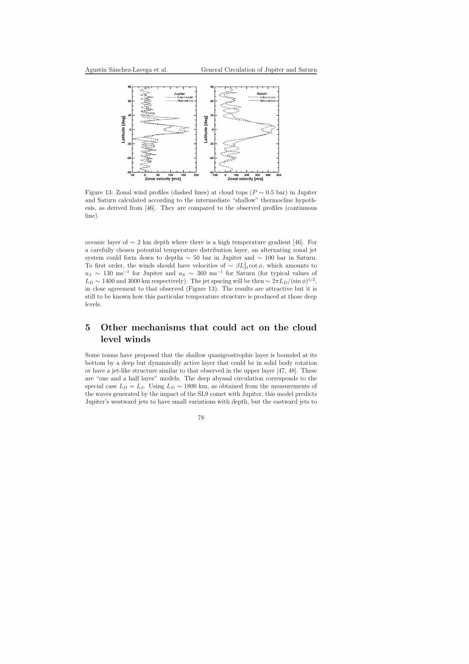
Agustın Sanchez-Lavega et al. General Circulation of Jupiter and Saturn
Figure 13: Zonal wind profiles (dashed lines) at cloud tops (P ∼ 0.5 bar) in Jupiterand Saturn calculated according to the intermediate “shallow” thermocline hypoth-esis, as derived from [46]. They are compared to the observed profiles (continuousline).
oceanic layer of ∼ 2 km depth where there is a high temperature gradient [46]. Fora carefully chosen potential temperature distribution layer, an alternating zonal jetsystem could form down to depths ∼ 50 bar in Jupiter and ∼ 100 bar in Saturn.To first order, the winds should have velocities of ∼ βL2
D cotφ, which amounts touJ ∼ 130 ms−1 for Jupiter and uS ∼ 360 ms−1 for Saturn (for typical values ofLD ∼ 1400 and 3000 km respectively). The jet spacing will be then ∼ 2πLD/(sinφ)1/2,in close agreement to that observed (Figure 13). The results are attractive but it isstill to be known how this particular temperature structure is produced at those deeplevels.
5 Other mechanisms that could act on the cloud
level winds
Some teams have proposed that the shallow quasigeostrophic layer is bounded at itsbottom by a deep but dynamically active layer that could be in solid body rotationor have a jet-like structure similar to that observed in the upper layer [47, 48]. Theseare “one and a half layer” models. The deep abyssal circulation corresponds to thespecial case LD = Lβ. Using LD ∼ 1800 km, as obtained from the measurements ofthe waves generated by the impact of the SL9 comet with Jupiter, this model predictsJupiter’s westward jets to have small variations with depth, but the eastward jets to
78
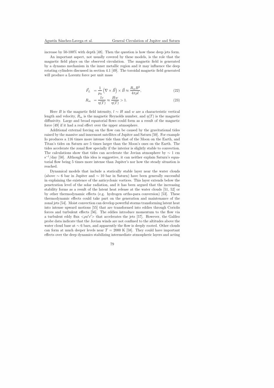
Agustın Sanchez-Lavega et al. General Circulation of Jupiter and Saturn
increase by 50-100% with depth [48]. Then the question is how these deep jets form.
An important aspect, not usually covered by these models, is the role that themagnetic field plays on the observed circulation. The magnetic field is generatedby a dynamo mechanism in the inner metallic region and it may influence the deeprotating cylinders discussed in section 4.1 [49]. The toroidal magnetic field generatedwill produce a Lorentz force per unit mass
~FL =1
µ0
(
∇× ~B)
× ~B ≈RmB2
4πρl, (22)
Rm =lv
η(T )≈
Hw
η(T )> 1. (23)
Here B is the magnetic field intensity, l ∼ H and w are a characteristic verticallength and velocity, Rm is the magnetic Reynolds number, and η(T ) is the magneticdiffusivity. Large and broad equatorial flows could form as a result of the magneticforce [49] if it had a real effect over the upper atmosphere.
Additional external forcing on the flow can be caused by the gravitational tidesraised by the massive and innermost satellites of Jupiter and Saturn [50]. For exampleIo produces a 116 times more intense tide than that of the Moon on the Earth, andTitan’s tides on Saturn are 5 times larger than the Moon’s ones on the Earth. Thetides accelerate the zonal flow specially if the interior is slightly stable to convection.The calculations show that tides can accelerate the Jovian atmosphere by ∼ 1 cms−1/day [50]. Although this idea is suggestive, it can neither explain Saturn’s equa-torial flow being 5 times more intense than Jupiter’s nor how the steady situation isreached.
Dynamical models that include a statically stable layer near the water clouds(above ∼ 6 bar in Jupiter and ∼ 10 bar in Saturn) have been generally successfulin explaining the existence of the anticyclonic vortices. This layer extends below thepenetration level of the solar radiation, and it has been argued that the increasingstability forms as a result of the latent heat release at the water clouds [51, 52] orby other thermodynamic effects (e.g. hydrogen ortho-para conversion) [53]. Thesethermodynamic effects could take part on the generation and maintenance of thezonal jets [54]. Moist convection can develop powerful storms transforming latent heatinto intense upward motions [55] that are transformed into eddies through Coriolisforces and turbulent effects [56]. The eddies introduce momentum to the flow viaa turbulent eddy flux <ρu′v′> that accelerates the jets [57]. However, the Galileoprobe data indicate that the Jovian winds are not confined to the altitudes above thewater cloud base at ∼ 6 bars, and apparently the flow is deeply rooted. Other cloudscan form at much deeper levels near T = 2000 K [58]. They could have importanteffects over the deep dynamics stabilizing intermediate atmospheric layers and acting
79

Agustın Sanchez-Lavega et al. General Circulation of Jupiter and Saturn
as opacity sources for energy transfer. They certainly should be considered in futuredynamical models.
6 Models of motions above the clouds
Different hypotheses have been suggested for the observed decrease of the wind pat-tern above cloud level (see section 3). One possible mechanism is that the upper flowdecreases with altitude due to the friction imposed on the mean zonal flow at cloudtop level. This process can be simulated by a parameterization of a dynamical balancebetween Coriolis forces and a Rayleigh friction drag, and by a thermodynamic balanceusing a Newtonian radiative damping [22, 23]. As a consequence, mass upwelling anddownwelling above the clouds must occur. This motion is part of a mean meridionaloverturning that balances the Coriolis acceleration and the vertical advection of tem-perature with the dissipative effects, i.e. fv ∼ u/τf , wHN2/Rg ∼ −∆T/τrad, whereτf is a characteristic damping time, w the vertical velocity and τrad the radiativedamping time. Another possibility is that the development of shear instabilities inthe stable layer above the clouds produce large-scale eddies that give the requireddecay of jets within the upper troposphere and provide a physical mechanism for theunderlying drag coefficient parameterization [59, 60, 61].
The dynamics in the upper troposphere and lower stratosphere is complicatedby the presence of large-scale waves and by the belt-zone temperature differencesproduced by the differential sunlight absorption of the aerosols. The aerosols arespecially abundant over the polar regions [62]. Models of the residual mean meridionalcirculation that take into account the solar deposition heating rates of the aerosols,result in an hemispheric-wide circulation cell (Hadley-like) that vertically extendsfrom 1 mbar to 100 mbar [63, 64]. A two-year tracking of the aerosol debris left bythe SL9 comet impact with Jupiter in 1994 supports the existence of a large meridionalhemispheric circulation, but unfortunately this circulation has a sign contrary to thepredictions of such models [65].
7 Laboratory Experiments
Several fluid dynamics experiments have been performed on ground and space-basedlaboratories aiming to simulate the general circulation on the giant planets. Manyothers have been done to simulate vortex formation, but these are not described here.Thermal convection experiments on a rapidly rotating sphere heated from below undermicrogravity conditions were performed by astronauts onboard the Spacelab [66, 67],confirming the formation of the columnar convection modes. Their experiments usedPr = 8, E = 2.6 × 10⁻³ and Racrit = 2000. Columnar motions taking place at
80

Agustın Sanchez-Lavega et al. General Circulation of Jupiter and Saturn
the onset of convection have been also observed on ground laboratories where thecentrifugal force is used to compensate the gravity [34].
A deep convection laboratory analog consisting of a rotating bowl of warm wateruniformly cooled at the free surface was demonstrated to generate convection cellsthat give rise to azimuthal jets when they encounter the free surface [68]. Symmetricbands and zonal jets in a rotating convecting fluid sphere have also been found forthe following values of the characteristic numbers: Pr = 6, E = 10−5 − 10−6 andRacrit ∼ 800. However a low velocity equatorial jet flowing westward forms contrarilyto what is observed in Jupiter and Saturn [69].
These results demonstrate that some features of the theoretical models can becaptured on laboratory experiences, but new careful experiments resembling as muchas possible the conditions on the giant planets interior (with respect to the values forPr, E and Racrit) must be performed. Experiments under microgravity conditionswould be specially useful (perhaps this could be an experience to develop in theInternational Space Station).
8 Final comments
One important point that can shed light on the general circulation is the study ofthe long-term temporal variability of the jet structure. A first simple argument isthat if the insolation forcing dominates, as expected in most “shallow” water models,then a planet like Saturn that suffers intense seasonal insolation changes, enhancedin the equator by the ring shadowing, should follow the sunlight cycle. Its zonal jetsystem should change in jet location and intensity as a response to seasons. Ourrecent observation of a drop in Saturn’s equatorial wind velocity could point in thisdirection [15]. However, the observed stability of the non-equatorial jets together withthe scarce available historical observations of Saturn’s winds suggest global long-termstability.
A second point is that we need details of the non-zonal component of the flow,including the momentum and heat transfer by eddies. In other words, we need toclarify what is the role the vortices and local motions (e. g. convective storms) play onthe zonal circulation. The equatorial wind drop of Saturn could be simply the resultof the large convective storm that erupted few years before the drop was detected.The change observed in the strongest jet of Jupiter [70] could have also been theresult of a large disturbance that occurred there [71]. The hemispherical asymmetryobserved between the tropical jets of Jupiter (compare the jets at latitudes 23S and23N in Figure 6) could be due to the presence of the Great Red Spot that modifiesthe jets by deflecting them meridionally. If this were the case, the presence of thevortices could play an important role in shaping and pumping the jets. However,Saturn lacks in number and size the kind of large vortices present in Jupiter (at least
81
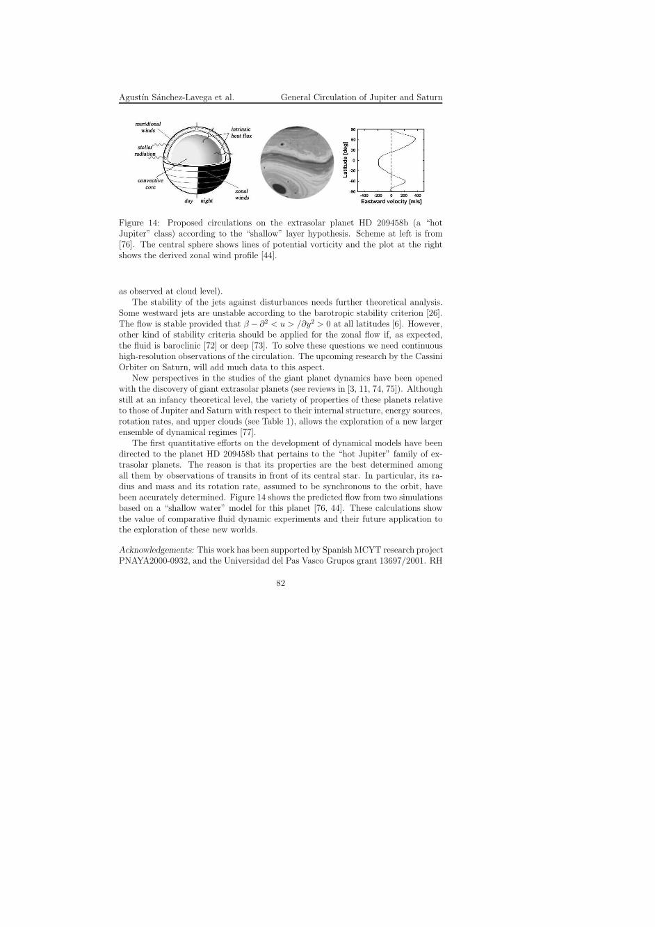
Agustın Sanchez-Lavega et al. General Circulation of Jupiter and Saturn
Figure 14: Proposed circulations on the extrasolar planet HD 209458b (a “hotJupiter” class) according to the “shallow” layer hypothesis. Scheme at left is from[76]. The central sphere shows lines of potential vorticity and the plot at the rightshows the derived zonal wind profile [44].
as observed at cloud level).The stability of the jets against disturbances needs further theoretical analysis.
Some westward jets are unstable according to the barotropic stability criterion [26].The flow is stable provided that β − ∂2 < u > /∂y2 > 0 at all latitudes [6]. However,other kind of stability criteria should be applied for the zonal flow if, as expected,the fluid is baroclinic [72] or deep [73]. To solve these questions we need continuoushigh-resolution observations of the circulation. The upcoming research by the CassiniOrbiter on Saturn, will add much data to this aspect.
New perspectives in the studies of the giant planet dynamics have been openedwith the discovery of giant extrasolar planets (see reviews in [3, 11, 74, 75]). Althoughstill at an infancy theoretical level, the variety of properties of these planets relativeto those of Jupiter and Saturn with respect to their internal structure, energy sources,rotation rates, and upper clouds (see Table 1), allows the exploration of a new largerensemble of dynamical regimes [77].
The first quantitative efforts on the development of dynamical models have beendirected to the planet HD 209458b that pertains to the “hot Jupiter” family of ex-trasolar planets. The reason is that its properties are the best determined amongall them by observations of transits in front of its central star. In particular, its ra-dius and mass and its rotation rate, assumed to be synchronous to the orbit, havebeen accurately determined. Figure 14 shows the predicted flow from two simulationsbased on a “shallow water” model for this planet [76, 44]. These calculations showthe value of comparative fluid dynamic experiments and their future application tothe exploration of these new worlds.
Acknowledgements: This work has been supported by Spanish MCYT research projectPNAYA2000-0932, and the Universidad del Pas Vasco Grupos grant 13697/2001. RH
82

Agustın Sanchez-Lavega et al. General Circulation of Jupiter and Saturn
thanks a post-doctoral fellowship from Gobierno Vasco. SPH acknowledges a PhDfellowship from Spanish MECD.
References
[1] Ingersoll, A.P. 1990, Science, 248, 308[2] Ingersoll, A.P., Dowling, T.E., Gierasch, P.J., Orton, G.S., Read, P.L., Sanchez-
Lavega, A., Showman, A.P., Simon-Miller, A.A., Vasavada, A.R. To appear in:Jupiter: The Planet, Satellites, and Magnetosphere (F. Bagenal, W. McKinnonand T. E. Dowling, Ed.) Cambridge University Press, (in the press)
[3] Burrows, A., Hubbard, W.B., Lunine, J.I., Liebert, J. 2001, Rev. Modern Phys.73, 719
[4] Sukoriansky, S., Galperin, B., Dikovskaya, N. 2002, Phys. Rev. Lett., 89, 124501[5] Hanel, R., Conrath, B., Herath, L., Kunde, V., Pirraglia, J. 1981, J. Geophys.
Res., 86, 8705[6] Ingersoll, A.P., Beebe, R.F., Mitchell, J.L., Garneau, G.W., Yagi, G.M., Muller,
J.P. 1981, J. Geophys. Res., 86, 8733[7] Limaye, S.S. 1986, Icarus, 65, 335[8] Garcıa-Melendo, E., Sanchez-Lavega, A. 2001, Icarus, 152, 316[9] Porco, C.C., and co-authors 2003, Science, 299, 1541
[10] Gierasch, P.J., Conrath, B.J. 1993, J. Geophys. Res., 98, 5459[11] Guillot, T. 1999, Science, 286, 72[12] A. R. Vasavada, A.R., Ingersoll, A.P., Banfield, D., Bell, M., Gierasch, P.J.,
Belton, M.J.S., Orton, G.S., Klaasen, K.P., De Jong, E., Breneman, H.H., Jones,T.J., Kaufman, J.M., Magee, K.P., Senske, D.A. 1998, Icarus, 135, 265
[13] Ingersoll, A.P., Beebe, R.F., Conrath, B.J., Hunt, G.E. 1984, Structure anddynamics of Saturn’s atmosphere, in Saturn, T. Gehrels and M. S. Matthews(eds.), University of Arizona Press, Tucson, 195
[14] Sanchez-Lavega, A., Rojas, J.F., Sada, P.V. 2000, Icarus, 147, 405[15] Sanchez-Lavega, A., Perez-Hoyos, S., Rojas, J.F., Hueso, R., French, R.G. 2003,
Nature, 423, 623[16] Sanchez-Lavega, A., Colas, F., Lecacheux, J., Laques, P., Miyazaki, I., Parker,
D. 1991, Nature, 353, 397[17] Barnet, C.D., Beebe, R.F., Conrath, B.J. 1992, Icarus, 98, 94[18] Sanchez-Lavega, A., Lecacheux, J., Colas, F., Laques, P. 1993, J. Geophys. Res.,
98, 18857[19] Peek, B.M. 1958, The Planet Jupiter, Faber & Faber, London[20] Rogers, J.H. 1995, The Giant Planet Jupiter, Cambridge University Press, Cam-
bridge[21] Beebe, R.F., Ingersoll, A.P., Hunt, G.E., Mitchell J.L., Muller, J.P. 1980, Geo-
phys. Res. Lett., 7, 1
83

Agustın Sanchez-Lavega et al. General Circulation of Jupiter and Saturn
[22] Gierasch, P.J., Conrath, B.J., Magalhaes, J.A. 1986, Icarus, 67, 456[23] Conrath, B.J., Gierasch, P.J., Leroy, S.S. 1990, Icarus, 83, 255[24] Atkinson, D.H., Pollack, J.B., Seiff, A. 1998, J. Geophys. Res., 103, 22911[25] Sromovsky, L.A., Revercomb, H.E., Suomi, V.E., Limaye, S.S., Krauss, R.J.
1982, J. Atmos. Sci., 39, 1433[26] Holton, J.R. 1992, An Introduction to Dynamical Meteorology, Academic Press,
San Diego[27] Showman, A.P., Ingersoll, A.P. 1998, Icarus, 132, 205[28] Showman, A.P., Dowling, T.E. 2000, Science, 289, 1737[29] Sanchez-Lavega, A. 1982, Icarus, 49, 1[30] Sanchez-Lavega, A., Lecacheux, J., Gomez, J.M., Colas, F., Laques, P., Noll, K.,
Gilmore, D., Miyazaki, I., Parker, D. 1996, Science, 271, 631[31] Busse, F.H. 1976, Icarus, 30, 255[32] Pedlosky, J. 1987, Geophysical Fluid Dynamics, Second Edition, Springer-Verlag,
New York[33] Busse, F.H. 1983, Pageoph, 121, 375[34] Busse, F.H. 1994, Chaos, 4, 123[35] Christensen, U.R. 2001, Geophys. Res. Lett., 28, 2553[36] Arnou, J.M., Olson, P.L. 2001, Geophys. Res. Lett., 28, 2557[37] Christensen, U.R. 2002, J. Fluid Mech., 470, 115[38] Zhang, K., Schubert, G. 2000, Science, 290, 1944[39] Guillot, T., Chabrier, G., Morel, P., Gautier, D. 1994, Icarus, 112, 354[40] Yano, J.I., Talagrand, O., Drossart, P. 2003, Nature, 421, 36[41] Williams, G.P. 1978, J. Atmos. Sci., 35, 1399[42] Cho, J.Y.K., Polvani, L.M. 1996, Science, 273, 335[43] Williams, G.P. 1985, Advances in Geophysics, 28, 381[44] Cho, J.Y.K., Menou, K., Hansen, B.S., Seager, S. 2003, ApJL, 587, L117[45] Williams, G.P. 2003, J. Atmos. Sci., 60, 1270[46] Allison, M. 2000, Planet Space Sci., 48, 753[47] Ingersoll, A.P., Cuzzi, J.N. 1969, J. Atmos. Sci., 26, 981[48] Dowling, T.E. 1995, Icarus, 117, 439[49] Kirk, R.L., Stevenson, D.J. 1987, ApJ, 316, 836[50] Ioannou, P.J., Lindzen, R.S. 1994, ApJ, 424, 1005[51] Barcilon, A., Gierasch, P.J. 1970, J. Atmos. Sci., 27, 550[52] Gierasch, P.J. 1976, Icarus, 29, 445[53] Smith, M.D., Gierasch, P.J. 1995, Icarus, 116, 159[54] Allison, M., Stone, P.H. 1984, Icarus, 54, 296[55] Hueso, R., Sanchez-Lavega, A. 2001, Icarus 151, 316[56] Hueso, R., Sanchez-Lavega, A., Guillot, T. 2002, J. Geophys. Res. Planets, 107[57] Ingersoll, A.P., Gierasch, P.J., Banfield, D., Vasavada, A.R. 2000, Nature, 403,
630[58] Fegley, B., Lodders, K. 1994, Icarus, 110, 117[59] Pirraglia, J.A. 1989, Icarus, 79, 196
84

Agustın Sanchez-Lavega et al. General Circulation of Jupiter and Saturn
[60] Orsolini, Y., Leovy, C.B. 1993, Icarus, 106, 392[61] Orsolini, Y., Leovy, C.B. 1993, Icarus, 106, 406[62] Moses, J.I., Fouchet, T., Yelle, R.V., Friedson, A.J., Orton, G.S., Bezard,
B., Drossart, P., Gladstone, G.R., Kostiuk, T., Livengood, T.A. To appear inJupiter: The Planet, Satellites, and Magnetosphere (F. Bagenal, W. McKinnonand T. E. Dowling, Ed.) Cambridge University Press, in press.
[63] West, R.A., Friedson, A.J., Appleby, J.F. 1992, Icarus, 100, 245[64] Moreno, F., Sedano, J. 1997, Icarus, 130, 36[65] Sanchez Lavega, A., Gomez, J.M., Rojas, J.F., Acarreta, J.R., Lecacheux, J.,
Colas, F., Hueso, R., Arregu, J. 1998, Icarus, 131, 341[66] Hart, J.E., Toomre, J., Deane, A.D., Hurlburt, N.E., Glatzmaier, G.A., Fichtl,
G.H., Leslie, F., Fowlis, W.W., Gilman, P.A. 1986, Science, 234, 61[67] Hart, J.E., Glatzmaier, G.A., Toomre, J. 1986, J. Fluid Mech., 173, 519[68] Condie, S.A., Rhines, P.B. 1994, J. Fluid Mech., 280, 349[69] Manneville, J.B., Olson, P. 1996, Icarus, 122, 242[70] Garcıa-Melendo, E., Sanchez-Lavega, A., Gomez, J.M., Lecacheux, J., Colas, F.,
Miyazaki, I., Parker, D. 2000, Icarus, 146, 514[71] Sanchez-Lavega, A., Miyazaki, I., Parker, D., Laques, P., Lecacheux, J. 1991,
Icarus, 94, 92[72] Dowling, T.E. 1995, Ann. Rev. Fluid Mech., 27, 293[73] Ingersoll, A.P., Pollard, D. 1982, Icarus, 52, 62[74] Perryman, M.A.C. 2000, Rep. Prog. Phys., 63, 1209[75] Hubbard, W.B., Burrows, A., Lunine, J.I. 2002, ARA&A, 40, 103[76] Showman, A.P., Guillot, T. 2002, A&A, 385, 166[77] Sanchez Lavega, A. 2001, A&A, 377, 354
85

Agustın Sanchez-Lavega et al. General Circulation of Jupiter and Saturn
86

ASTRONOMICAL TELESCOPES AT THE
TURN OF THE CENTURY
JOSE M. RODRIGUEZ ESPINOSAInstituto de Astrofısica de Canarias, E-38200 La Laguna, SPAIN
Abstract: The final years of the XXth Century and the initial years of the XXIstCentury are witnessing a revolution in the construction of large telescopes. This hasbeen possible thanks to the availability of both thin mirror technologies and largecomputing power. Astronomy is thus benefiting from this. Indeed the turn of thecentury has been rich with new discoveries, from the detections of extrasolar planetsto the discovery of the the farthest galaxies ever seen or the detection of accelerationin the expansion of the Universe.
Spain is leaving her imprint on the telescope making revolution and is promotingthe construction of a 10.4 metre telescope in the “El Roque de Los Muchachos”observatory, on the Island of La Palma, Spain. The Gran Telescopio Canarias (GTC)is currently at an advanced stage of construction, with science operation expected tostart early in 2006.
1 Introduction
Modern technology telescopes started to be made at the turn of the XIX centurywhen precision mechanics and precision optics started to be common use. In thepast, telescopes suffered from poor optics, as optical glasses were very difficult tomanufacture, and aluminization techniques were far from perfect. Nonetheless As-tronomy had continued its advance during the XIX century. This was the centuryof the stellar catalogues, the initial steps in stellar spectroscopy, with the generalizeduse of photographic plates.
The beginning of the XXth century brought us the HR diagram and the first at-tempts to study the stellar evolution. In the 20’s, the Curtis-Shapley controversy onthe size of the Milky Way was resolved and astronomers realised that the Universe wasa few orders of magnitude larger than previously thought. At that time the recentlybuilt Mt. Wilson 2.5m telescope was used to observe galaxies and with it Hubble dis-covered the general expansion of the Universe. Extragalactic Astronomy was startingprompting the construction of a 5 metre telescope a top Palomar Mountain to put ona firmer basis the expansion claim by observing the farthest galaxies. The Palomar
87

Jose M. Rodrıguez Espinosa Astronomical Telescopes
5m telescope was finished in 1945, in the midst of the European War. The Hale 5mtelescope, as the Palomar telescope was later known, has been one of the pillar of thedevelopment of astronomy during the XXth Century. Much of the theory of StellarNucleosynthesis was based on observation done with the Hale telescope. The discov-ery of the Quasars was also done with this telescope. The Hale telescope also set thestandards for telescope making technology, later followed by many other telescopesbuilt around the world.
2 Progress in Telescope Making
A key aspect that I would like to stress at this point is that the construction of newand better telescopes has been fundamental in the advancement of astronomy. Newand better telescopes and instruments have always resulted in clear advances in mostif not all branches of Astronomy.
It is interesting to note that as the XXth Century advanced new telescopes weregetting built, however with no increase in the size of their primary mirrors. Severaltelescope built from the 50’s to the 80’s include the Shane 3m telescope at Lick, theCrimean 6 m telescope, the Kitt Peak 4m telescope, the ESO 3.6 m in La Silla, theGerman 3.6 m telescope in Calar Alto (Spain), the Anglo-Australian and the WilliamHerschel 4m telescopes in Australia and at La Palma respectively, amongst others.
Except for the Crimean 6m telescope, it is interesting to note that most othertelescope built during the XXth Century were of the so called 4m class. Astronomywas advancing though at quite a fast pace, with the discovery of AGNs and quasars,the most luminous objects known to date, or the many advances in the study of thechemical abundances in many different kinds of galaxies and environments. Howeveras I say, all this progress was being made with 4m class telescopes.
The important aspect to notice is that the photon collecting power of these tele-scopes was being increased enormously. Not by making the telescopes bigger but bymaking the focal plane instruments more efficient and sensitive. This was so becausein the early XXth century the most common detector used was the photographicplate. Around that time, advances in electronic devices resulted in a large improve-ment of the performance of detectors. First phototubes, and photonmultipliers, latersemiconductor devices such as the Charge Coupled Devices, resulted in almost twoorders of magnitude increase in detecting power, or quantum efficiency as it is gen-erally known. Indeed the quantum efficiency of detectors was augmented from a fewpercent for photographic plates to almost 99% for modern CCD arrays. This wascombined with the availability of panoramic arrays, allowing multi-object capabili-ties, or wide area surveys. The clear advantage for astronomy was that even if the sizeof telescopes did not increased, astronomers were having a bonus in the improvementof detector devices.
88

Jose M. Rodrıguez Espinosa Astronomical Telescopes
In parallel, telescopes were being made better. Telescope mechanics was greatlyimproved with the use of Horizontal Mounts. These provided better mechanical sta-bility for pointing and tracking, offering at the same time large Nasmyth platforms forthe location of both heavy and sturdy high resolution spectrographs that allowed thestudy of lines profiles with unprecedented resolution. Horizontal mounts were knownfrom several centuries back. Their astronomical use was however not widespread dueto the complexity of the motion involved in tracking objects in the sky, necessary tocorrect for the motion of the Earth. Not until the advent of powerful enough comput-ers was it possible to perform real time computations of the positions of the telescopeaxes required to follow a given object on the sky.
Summarizing, from the mid 40’s to the mid 80’s, Astronomy advanced at a greatpace while the size of the telescopes remained rather constant at a canonical size ofabout 4 meter for the primary mirror. During this time the great development was indetector technology that evolved from photographic plates with quantum efficienciesof a few percent, to electronic devices bringing the quantum efficiency to almost 100%.Detectors also were enlarged in size from single unit detectors to arrays reachingseveral millions detectors per device. Science instruments benefited also from theavailability of new detectors. New and much better instruments were therefore builtfor the 4m class telescopes. These allowed the fast advancement of astronomy thatwas made during the XXth century.
Telescope making also progressed. Mechanical precision was substantially im-proved. Optical fabrication and finishing, as well as metrology were also greatlyimproved in the interim. Finally, electronics, software and control did really come ofage, thus setting up the stage for the revolution that was about to come in the lastyears of the XXth century.
3 Thin Mirrors
In the mid 80’s it was clear that further advances in Astronomy required furtherincreases in light gathering power. QSO research demonstrated that these were thenuclei of very faint galaxies that were very difficult to detect. QSO’s were also theobjects with the highest redshift known. QSO’s were nonetheless pathological objects.If the high-z Universe was made of QSOs only it would have been difficult to reconcilethe present day Universe with the high-z Universe. Therefore, it was clear that largerand more powerful telescopes were needed to, amongst other things, detect faint“normal” galaxies at high-z.
The road to higher quantum efficiency detector had already been explored. Fur-ther improvements in detector would come from either larger panoramic formats,better cosmetic or less electronic noise. However, even if these improvements wereindeed welcome, the gain in actual photon collecting power would not be of order of
89

Jose M. Rodrıguez Espinosa Astronomical Telescopes
magnitude, as would be required for the kind of Astronomy that people were tryingto do.
Astronomy thus demanded larger telescopes. Telescope making technology hadbeen largely improved in the past 50 years or so. Perhaps, the only stumbling blockwas the fact that increasing the size of primary mirrors had to be done not at theexpense of heavier mirrors, as this would have resulted in much heavier mechanicalstructures that would have been poised to wild flexure problems.
The solution to this impasse came from the great creativity and insight of peoplelike Jerry Nelson in California who proposed the use of thin mirrors. Thin mirrorshad the great advantage of being much lighter and the disadvantage of being fairlydeformable, requiring some active mechanisms for maintaining the optical figure asrequired, both when the mirror is static and against deformation by gravity as themirror is changed in position.
Fortunately, the technology was ready to take up the challenge of actively con-trolling the shape of thin mirrors. Realising this was Nelson’s greatest achievement.The road was therefore open to new increases in telescope sizes.
The late 80’s were full of enthusiasm for the design of larger telescopes both inthe US and in Europe. Thin mirror technology was indeed the default, althougha large spree of technological developments were necessary before these ideas couldbe put into practice. These included polishing large thin mirrors, or in the case ofsegmented mirror, polishing off-axis powered mirrors. The segmented approach wasdeveloped by Jerry Nelson during the conceptual design of the Keck telescope. InEurope the prefered approach was to produce large monolithic thin meniscus mirrors.The support strategy was common to both. The mirror production strategy was verydifferent though.
By the early 90’s both in the US engineers were advancing in the constructionof the Keck telescope, a 10 metre segmented primary telescope, and in Europe thecanonical project was the VLT, an array of 4 eight meter telescopes to be located inChile. Soon there was also the GEMINI partnership (UK, US, Argentina, Brazil andChile), two eight metre meniscus type telescopes to be placed both in Hawaii andChile, as well as the SUBARU telescope, a Japanese 8 metre meniscus telescope thatwas also to be located in Hawaii. Quite an impressive number of eight to ten metretelescopes at once!
The first of these telescopes to enter in operation was the Keck telescope. It wasalso the first large telescope to install a segmented primary mirror, and thereforeto have solved all the difficulties related with the alignment and phasing of the 36segments making up the full primary mirror. The success of this first large telescopewas such that it prompted the Keck Foundation to fund a second one with the goalof making optical and infrared interferometry. Yet a step forwards towards increasingthe spatial resolution of the observations.
Soon thereafter the European VLT, the Japanese SUBARU and the international
90

Jose M. Rodrıguez Espinosa Astronomical Telescopes
GEMINI projects commissioned its first telescopes. In a few years, the total collect-ing area had increased several times the total collecting area ever built in the past.Results from these telescopes appeared immediately after their commissioning. Highredshift galaxies, extrasolar planets, brown dwarfs, high-z supernovae, etc. Resultsthat have put Astronomy in the first pages of mass media. Results, like the accel-erated expansion of the Universe, obtained through the observation of high redshiftsupernovae, that have been considered by the US scientific journal “Science” one ofthe major physics discoveries of the decade.
4 The Spanish 10 metre telescope
In this scenario of excitement for new discoveries, Spain, through the pro-active pro-motion of the Instituto de Astrofsica de Canarias, started what will be the first Eu-ropean large segmented telescope. By the time of the Spanish decision to embark onthe construction of a large telescope both approaches, the segmented and monolithicmeniscus ones, had been demonstrated although only the Keck had recently startedoperation.
Prior to this, Spain, or rather the IAC had worked in a monolithic meniscus typeeight metre telescope project together with the UK. This project, which was carriedout till the production of a conceptual design document, was however abandoned whenthe UK joined forces with the US to constitute the GEMINI consortium. The IACnonetheless insisted in pursuing the idea of having a large telescope in its observatoryand continued its development work for controlling thin mirrors. Equally importantlythough was the formation at the IAC of a group of scientists and engineers whoseaim was the promotion and initial design of a Spanish large telescope.
This group produced a first design of a eight metre meniscus type mirror and calledon a group of international experts to review the concept and make recommendationsto pursue the idea of building a large telescope in Spain. It is interesting to notethat the review panel consisted of the top leaders of the large telescopes projects thenin the making. The panel was chaired by Paul Murdin, who had been in charge ofthe commissioning and first years of operation of the Williams Herschel telescope inLa Palma. Jerry Nelson, from the Keck telescope, was also in the committee, andhe represented the only large telescope that had started operation by then. Othermembers in the panel included Matt Mountain from GEMINI, Massimo Tarenghi,from VLT, Masanori Iye from SUBARU, John Hill, from LBT, and Arne Ardebergfrom the NOT telescope. Soon after this meeting the idea of changing the project toa segmented telescope instead was taking shape.
The final decision to promote a segmented 10 metre telescope was taken after thevisit of a group of scientists and engineers to the US to visit the Keck facilities, aswell as some of the contractors that had participated in the production of the Keck
91

Jose M. Rodrıguez Espinosa Astronomical Telescopes
mirror segments.
Reason for the change of concept were diverse. Certainly the success of the Kecktelescope was taken into a account. However other considerations were also important.For instance, the difficulty in bringing a monolithic meniscus through the narrow andwinding road to the observatory weithed heavily on the decission. The thought thata 10 metre segmented primary mirror telescope could be done for about the sameprice tag as an eight metre monolithic thin meniscus one was also important. Finally,although not considered at that time, it was soon realised that any future largertelescope would have to be segmented, thus Spain would be in a very good positionfor contributing actively to future large telescopes.
5 THE GTC
The Gran Telescopio Canarias (GTC) will be an advanced telescope when it entersoperation at the Observatorio del Roque de los Muchachos (ORM) in the island of LaPalma. It will carry a segmented primary mirror, consisting of 36 hexagonal segments.The secondary mirror will be a light weighted hexagonal mirror made of beryllium.The GTC will carry a third mirror, the tertiary mirror to fold the light beam to anyof the Nasmyth or the folded Cassegrain foci. The optical desigh of the GTC is aRitchey-Chretien with an effective focal ratio of f/17. This results in a focal planescale of 1.21 arcsecond per millimetre.
6 The GTC: Status and perspectives
The Gran Telescopio Canarias (GTC) is currently being assembled at the ORM in LaPalma. First light is expected for mid 2005 with the first science observations expectedby mid 2006. As of this writing the enclosure, building and dome, are finished, withminor problems pending. These are related to the shutter motion and the ventilationwindows. Solutions for fixing the problems exist already to be implemented by thesummer 2004.
By the time the telescope is turned to the operation team, the two Nasmythplatforms will have been commissioned together with two science instruments (CA-NARICAM and OSIRIS/ELMER).
For the time being, the main milestones are the completion of the telescope mountinside the dome, the reception of the first batch of segments, the acceptance of boththe Acquisition and Guiding boxes and the Commissioning Camera. Further tasksfor the immediate future are the start of the Astronomy operation group and theintegration of the first science instruments. These first two instruments will providethe GTC with capabilities for low resolution multi-object spectroscopy, imaging in
92

Jose M. Rodrıguez Espinosa Astronomical Telescopes
both lines and continuum in the optical and mid infrared, as well as polarimetry and,for the first time ever, coronagraphy in the mid infrared.
6.1 Enclosure
Work inside the enclosure is progressing. Offices are being furnished and labs are beingsupplied with their necessary equipment. The air conditioning system is workingnormally.
The GTC enclosure has been provided with 32 ample independently operatedventilation windows, allowing for 432 squared metre of clear opening spaces, to helpmaintain a laminar flow of air during the night. This is important to keep the insidetemperature equal to the outside temperature, thus reducing temperature gradientsthat may degrade the quality of the images produced by the telescope.
Figure 1: GTC enclosure showing the ventilation windows in three rows.
The azimuth pier is ready to take up the azimuth ring. As of this writing theazimuth ring is being mounted and adjusted. Figure 2 shows the interior of the domewith the azimuth pier in the centre. Figure 3 shows the azimuth ring already set overthe pier.
6.2 Telescope Mount
Once all homogeneity, roughness, eccentricity, etc. tests are finished for the azimuthring, the rest of the telescope will continue being mounted. Most major pieces of thetelescope structure are at the site waiting to be installed. Those not needed in the
93

Jose M. Rodrıguez Espinosa Astronomical Telescopes
Figure 2: Interior of the dome showing the azimuth pier.
immediate future are still undergoing tests in their respective factories. That is thecase for instance of the instrument rotator bearings (Figure 4).
Next steps in the mounting process will consist of the installation of the hydrostaticbearings and the rotating floor, allowing to test the azimuth rotation. Once this isachieved the azimuth encoder tape will be installed, and in parallel the yoke of thetelescope will be erected, to continue with the elevation ring and mirror cell, theelevation trunnions and Nasmyth platforms, the tertiary tower, upper tube, spiderring and secondary support structure. This will take the rest of 2004 and some timein 2005.
By then, and once the necessary performance tests are satisfactorily passed, thetelescope will be ready to take up the optics.
6.3 Telescope Optics
All 36 (+6 spare) segment blanks are fabricated. Made of Zerodur by SCHOTT, theirmeasured properties comply with the specifications in all respects, in particular interm of low thermal coefficient of expansion and homogeneity of this coefficient.
The segment blanks are now at SAGEM, near Paris, where they are being polished.The polishing process is a lengthy and complicated one due to the extreme accuracyrequired to meet the strict image quality requirements of the GTC.
The secondary mirror is also being polished after a complicated blank productionprocess in which several blanks were broken. The secondary mirror is made out ofBeryllium as it needs to be very light while being fairly rigid. The GTC secondarymirror (Figure 5) is an important part of the telescope as it defines the entrance aper-
94

Jose M. Rodrıguez Espinosa Astronomical Telescopes
Figure 3: The azimuth ring on top of the pier.
Figure 4: Instrument rotators bearings being tested.
ture of the telescope. This is to maintain low thermal emissivity for better infraredperformance of the telescope. The secondary mirror has five degrees of freedom, tomaintain the correct alignment between the primary and secondary mirrors when thetelescope changes elevation, to perform fast guiding and to correct for wind buffetingon the telescope structure, and finally to perform chopping for infrared observations.
Other important optical systems include the Tertiary mirror that is being polishedin Moscow and it is expected to be finished by mid 2004, the Commissioning Camera,that is being made in Mexico and is about to be completed, and the Acquisitionand Guiding (A&G) boxes. Both the Commissioning Camera and the A&G boxesare complicated subsystems, employing several cameras (Figure 6) as well as severalwavefront sensing devices. The Commissioning Camera is meant to help during theinitial alignment and phasing of the primary mirror segments. The A&G boxes willbe in charge not only of acquiring the object to be observed and keeping it within
95

Jose M. Rodrıguez Espinosa Astronomical Telescopes
Figure 5: Secondary mirror.
Figure 6: One of the arms of the Acquisition and Guiding boxes. The picture showsthe optics inside this arm.
the aperture of the instrument, which is the classical use of the A&G boxes, but alsowill perform wavefront sensing to regularly monitor the status of the telescope optics.This is an advantage with regards to the Keck telescopes. These can not performwavefront sensing on real time except when their Alignment Camera is installed,which is not always the case.
6.4 Software and Control
The GTC will be controlled by an overall software system that sees the GTC as asingle unit. Every subsystem will be included in this software, from the dome and thedifferent equipment in the dome to the telescope, optics, instruments, and includingthe data acquisition and processing pipelines from the moment a proposal is submitted
96

Jose M. Rodrıguez Espinosa Astronomical Telescopes
by an astronomer to the moment the data are sent to the astronomer and archivedin the GTC archive. The control system is therefore key to the successful operationof the GTC.
Of great interest for astronomers is every thing that is related with the scienceinstruments and the scientific data. The software for generating the observing pro-posals is quite advanced, with test versions already available. This software will usea scheme of two phases. Phase II will be used by those astronomers granted time bythe different allocation committees, to introduce enough details of their observationsto produce the observing blocks that will be used by the observatory staff to performthe observations.
The control system includes data reduction pipelines, consisting of a basic reduc-tion pipeline and a more advanced data reduction. The basic reduction is meant tocorrect those effects that are originated in the detector arrays, i.e. bias, dark current,flats, cosmetic, etc. Then, depending on the observing mode, there may be a moreadvanced pipeline that might perform wavelength calibration and a spectral extrac-tion. This software may be of valuable use for the astronomer, at least to make anassessment of the data present in the archive. The software is also of good use forthe observatory crew to ascertain the quality of the observation being done duringthe night, and indeed for monitoring the performance of the instruments.
7 The Science Instruments
The GTC will be equipped with a suite of facility instruments presently under con-struction. The first generation instruments will be OSIRIS and CANARICAM. Athird instrument under construction, ELMER, is a backup instrument meant to beused if the main instruments are not on time when they are required at the telescope.
A instrument belonging to the second generation of facility instruemns, EMIR, hasbeen started, so that there is not a big gap between the arrival of the first instruments,and that of the second generation. To complete the picture, some visiting instrumentsthat have been proposed will be mentioned. These are CIRCE and UES.
In what follows there is a brief description of these instruments.
7.1 OSIRIS
OSIRIS is instrument whose primary design goal is to perform wide field (8’ x 8)optical imaging with tuneable filters, therefore being specially suited for performingsurveys and detailed studies of emission line objects. OSIRIS will also be capable ofperforming low resolution spectroscopy (R= 500 to 2500), both multi-object and longslit, as well as fast photometry and spectrophotometry.
OSIRIS will be equipped with two modern 2Kx4K CCD arrays, with frame transfer
97

Jose M. Rodrıguez Espinosa Astronomical Telescopes
Figure 7: A drawing of OSIRIS showing its main parts.
capabilities, allowing observations of the line and continuum, followed by on chipsubtraction before reading out the array, therefore substantially reducing the noise.
OSIRIS is a project led by Jordi Cepa, from the IAC, with strong collabora-tions from the Institute of Astronomy at the UNAM (Mexico) and the University ofCantabria (Spain). OSIRIS will be an excellent instrument to study the evolution ofgalaxies both in clusters and in the field, as well as detailed observations of nearbygalaxies. Figure 7 shows a drawing with the main parts of OSIRIS marked. OSIRISis in a fairly advanced state of construction. Integration is expected to start in thesecond half of 2004, with completion expected by June 2005, well in time of beinginstalled at the telescope for tests and commissioning.
OSIRIS should be able to reach 26 magnitude objects in the r (SDSS) band witha signal to noise ratio of 5 in 1000 seconds. In spectroscopy, OSIRIS should be ableto observe objects of magnitude between 20.5 and 22 depending upon the wavelengthand the dispersion employed.
7.2 CANARICAM
CANARICAM is a thermal infrared instrument being built at the University ofFlorida, Gainsville. Charlie Telesco is the Principal Investigator. Charlie Telescois very well known for the constructions of several first class thermal IR instrumentsboth for space and the ground. CANARICAM will be capable of performing imag-ing, spectroscopy, polarimetry and coronagraphy in the mid IR bands from 8 to 25micron. CANARICAM will be specially suited for observing brown dwarfs and ex-trasolar planets, as well as dust enshrouded objects like protostars, regions of star
98

Jose M. Rodrıguez Espinosa Astronomical Telescopes
formation, and high redshift star forming galaxies.CANARICAM is fairly advanced with most optical components already fabri-
cated. The cryostat (Figure 8) is undergoing tests, and will be ready to start in-tegrating all components soon. CANARICAM is expected to be delivered in June2005.
Figure 8: The CANARICAM dewar undergoing tests in the laboratory.
CANARICAM will be able to observe point sources as faint as 30 µJy (S/N= 1in 1 hour) in the 10 µ band or perform line spectroscopy of objects with 0.7 x 10⁻¹⁸
W m−2 with the high resolution grating (R ∼ 1300).
7.3 ELMER
ELMER is an instrument for performing imaging and low to intermediate resolutionspectroscopy in the optical range. With a field of view of over 3 x 3 arcminutes squaredELMER is optimised for maximum throughput. The design of ELMER (Figure 9)has been made in such a way as to minimise risks maintaining a tight budget.
ELMER is advancing quite satisfactorily under the leadership of Marisa GarcıaVargas, from the GTC Project Office. ELMER will perform imaging with conven-tional narrow and broad band filters, and low resolution (R= 500) spectroscopy withprisms, medium resolution (R=1500) spectroscopy with grisms, and relatively high(R= 5000) resolution with Volume Holographic Prisms.
ELMER is also capable of performing fast photometry as well as fast spectropho-tometry. This is achieved, as in OSIRIS, by using the charge transfer capability ofthe array detectors combined with adequate masks and a clocking strategy for fastshifting of the charge up in the array.
99

Jose M. Rodrıguez Espinosa Astronomical Telescopes
Figure 9: Drawing of ELMER showing the main parts and the compact design.
It is expected that ELMER will attain very high sensitivities. Current estimationsprovide figures like 26.8 magnitude in the r band (S/N: 5 in 1 hour with 1 arcsecondseeing). For spectroscopy the expected sensitivity is 20-22 magnitude (depending onwavelength) for a S/N= 20 under 0.6 arcsecond seeing in 1 hour.
ELMER is designed to be eventually installed at one of the GTC Folded Cassegrainfoci, providing therefore an excellent standby instrument for imaging and spectroscopyeven when the primary instrument may be any other of the GTC facility instruments.
7.4 EMIR
Figure 10: Drawing of EMIR showing the main parts and the compact design. Theouter shield is a cryostat
100

Jose M. Rodrıguez Espinosa Astronomical Telescopes
Figure 11: Prototype of the EMIR slit mask unit. Note the sliding blades that makeup the slit of the desired size.
EMIR is a wide field multi-object cryogenically cooled near IR spectrograph (Fig-ure 10). EMIR is being designed and fabricated at the IAC under the leadershipof Francisco Garzon, with strong collaborations from the Universidad Complutensede Madrid and the Observatoire de Midi-Pyrenees. The design of EMIR is drivenby COSMOS, a scientific project which aim is to make a census of the star forminggalaxian population out to redshift 2.5, in order to set quantitative limits to the starformation density when the Universe was much younger than it is now.
EMIR will perform imaging and spectroscopy from 1 to 2.5 µm. Key features inEMIR are the very wide field of vision, 6 x 6 arcminutes squared, and the relativelyhigh resolution required to perform an adequate subtraction of the OH telluric lines.EMIR will perform multi-object spectroscopy with masks that will be cryogenicallycooled. One of the challenges of EMIR is to produce a mask changing mechanismthat does not involve warming up and cooling down the instrument every time thatthe masks need to be changed. The current baseline for EMIR is to implement arobot (Figure 11) that will be in charge of producing the masks whenever needed.This robot will use a set of cryogenically cooled sliding blades that can be softwarecontrolled. EMIR is expected to be completed by the end of 2006.
7.5 Visiting Instruments
The GTC is adopting a policy for visiting instruments in order to fill some niches notcovered by the initial facility instruments. There are several instruments that havebeen proposed as visiting instruments. Perhaps the two more interesting ones areCIRCE and UES.
CIRCE is a near IR camera that will fit into one of the Folded Cassegrain foci.CIRCE will be provided by the University of Florida and will add near IR capabilities
101

Jose M. Rodrıguez Espinosa Astronomical Telescopes
to the GTC before the arrival of EMIR.
UES is a high resolution echelle spectrographs that has been in use at the WilliamsHerschel telescope fore more than ten years. UES has been recently decommissioned.Ramon Garcıa Lopez from the IAC is leading the conversion of UES to the GTC,through a fibre plus micro lenses link. UES will be upgraded with new coatings, newdetectors and new software. UES will provide high resolution (R 50000) to the GTC.
8 Adaptive Optics
The quest for image quality can be taken beyond the optics of a given telescope. Oncea telescope is built with precise requirements on the quality of the optics, reality tellsthat the atmosphere is then the limiting factor dictating the image quality obtainedon the array detectors. This is commonly known by the term “seeing limited” images.Space telescopes on the contrary are limited by the quality of their optics, or in otherwords, they produce diffraction limited images.
Ground based telescopes are actively working on methods to circumvent the atmo-sphere in their quest for image quality. One method that is actively being developedis “Adaptive Optics”. Adaptive Optics is a technique that tries to correct for tur-bulence in the atmosphere therefore producing nearly diffraction images. There aretwo main elements to an adaptive optics system, namely the characterization of theturbulence pattern in the atmosphere and the reconstruction of the corrected lightbeam. The first one requires the availability of a bright enough reference source. Thesecond one is done with a deformable mirror that produces positive or negative phaseshifts in the footprint of the beam in order to flatten it out.
The first part is achieved with a wavefront sensor that analyses that light from thereference source on almost real time, thereby determining the aberrations that thelight beam carries after its passage through the atmosphere. The measurements needto be done relatively fast as the atmosphere is constantly changing. This requiresa relatively bright source close to the object of interest. This is not always possibleand in order to increase the fraction of sky over which the correction can be madeartificial laser reference stars are produced. This is technique that has been testedsatisfactorily, however the availability of sufficiently powerful lasers is still a problem.
Once the signal has been processed by the wavefront sensor and the aberrationshave been determined the loop is closed with the deformable mirror, and this isprogrammed in such a way as to correct the beam. Deformable mirror technology isadvancing quite rapidly.
The GTC has a Adaptive Optics programme, still in the design phase, that willallow for adaptive correction of the beam, delivering corrected images in the J, H andK bands. The baseline is to have an Adaptive Optics system by early 2007, to be usedwith natural reference stars. This initial system will be upgradeable to its use with a
102

Jose M. Rodrıguez Espinosa Astronomical Telescopes
laser reference star system, and subsequently further upgraded with the utilization ofa second deformable mirror. This produces better correction and a larger and morehomogeneously corrected field.
9 The Future
The Kecks in the States and the GTC in Spain will be the only segmented telescopeswith strict image quality requirements produced so far. Future large telescopes how-ever will also be segmented. Thus the technology demonstrated by the Kecks andmuch improved by the GTC will be instrumental for the development of future largertelescopes.
The construction of larger telescopes is also very much dependent on the availabil-ity of adaptive optics. This is mostly because the size of the focal plane instrumentsgrows with the size of the telescope except in the case of telescopes that are diffractionlimited. Large telescopes will also be very much dependent on the active correctionof its optics. This will be complicated due to the large number of segments requiredto fill a large aperture. Indeed large telescopes are truly challenging projects.
There are at present several very large telescope projects. Most of these projectsare still at a very preliminary stage of development. Some do not even have fundsto go beyond a more or less detailed design stage. However the name of the gameis telescopes of sizes ranging from 30 to 100 metre that should be ready in the nextdecade.
The most advanced project is perhaps the California Extremely Large Telescopeor CELT, which is led by Jerry Nelson from the University of California. CELT isa partnership of the University of California and Caltech. Also in the US there isthe Giant Segmented Mirror Telescope (GSMT ) concept, a 30m telescope projectpromoted by the AURA New Initiatives Office. In Europe there are two projects witha very differing approach. The EURO50 is a 50 metre aspheric primary telescope,very much along the design lines of the US projects CELT and GSMT. EURO50 isbeing promoted by the Lund telescope group with participation of groups from otherEuropean countries like Spain, Ireland and the UK. The second European project isthe OverWhelmingly Large (OWL )telescope. The baseline is a 100 metre sphericalprimary telescope.
All these projects are expensive, with price tags ranging from 700 to 1000 M.Whether one or more of these very large telescopes is made is still to be seen. Theodds favour the CELT, which with private funds is progressing quite fast in its designstage. Europe is lagging behind for lack of funding. Two outcomes are possible.Either the European Union come up with a fair fraction of the funds required, orthere is a world wide effort to converge to a single project.
103

10 Summary
The GTC is a 10m telescope currently being built in La Palma, Spain. The GTC is acollaboration between Spain (90%), Mexico (5%) and the University of Florida (5%).The expected day for completion of the project is May 2006, after several difficultieshave resulted in some delay. A set of facility instruments will be ready by then. I doexpect that the GTC will be an outstanding telescope at the disposal of the Spanish,Mexican and Floridian astronomical communities.
Acknowledgements: I am grateful to Profs. Minia Manteiga and Ana Ulla for theorganisation of the Astronomy session in the Centennial Meeting of the Real SociedadEspanola de Fısica. I am also grateful for their patience in waiting for this manuscript.Ana Perez was, as always, of great help with the Latex manuscript.
104

FULLERENES AND BUCKYONIONS IN THE
INTERSTELLAR MEDIUM
SUSANA IGLESIAS GROTHInstituto de Astrofısica de Canarias, E-38200 La Laguna, SPAINDepartamento de Fısica Fundamental II, Universidad de La Laguna, E-38204 LaLaguna, SPAIN
Abstract: We have studied the contribution of single fullerenes and buckyonionsto the interstellar extinction. The photoabsorption spectra of these molecules ispredicted and compared with some of the most relevant features of interstellar ex-tinction, the UV bump, far UV rise and the diffuse interstellar bands. We concludethat fullerenes and buckyonions may explain these features and make a preliminaryestimate of the carbon fraction locked in these molecules.
1 Introduction
The most prominent feature in the interstellar medium extinction curve is the UVbump at 2175 A. The carrier of this band has been frequently associated to someform of carbonaceous material (graphitic spheres, polycyclic aromatic hydrocarbons(PAHs), hydrogenated amorphous carbon, etc.) but there is no definitive conclusionon the ultimate responsible for the band. The increase in the extinction at higherenergies and the existence of many much weaker diffuse interstellar bands (DIBs)in the optical [1] of unknown origin are also some of the intriguing observationalproperties of the interstellar material. Recently, it has been claimed the detection offullerenes with 60-240 carbon atoms in the Allende and Murchison meteorites [2]. Thisis the first direct indication that fullerenes were present in the presolar nebula andstrongly support previous suggestions [3] that fullerenes may exist in the interstellarmedium.
In this work, we study the possible contribution of single fullerenes and bucky-onions (multishell fullerenes) to the interstellar extinction. We predict their photoab-sorption spectra and we compare the main features of these spectra with some of theobservational properties of interstellar extinction, in particular with the characteris-tics of the UV bump and with the distribution of diffuse interstellar bands (DIBs) inthe optical and near infrared.
105

Susana Iglesias Groth Fullerenes and Buckyonions
2 General properties of fullerenes
Figure 1: Buckyonion C60@C240
The arquetype of the icosahedric fullerenes is the C60 a closed cage formed by 60carbon atoms distributed on the surface of a sphere of radius ∼ 3.55 A following thesymmetry of a truncated icosahedrum. In 1970, Osawa suggested that a moleculewith this geometry would be chemically stable. In this molecule, each carbon atomwith four valence electrons is bounded to the three nearest carbon atoms. Twoof the bounds are single and link a hexagon with a pentagon, the third is doubleand links two hexagons. The molecule is formed then, by 30 double and 60 singlebounds. The distances between atoms in single and double bounds are 1.45 and 1.37A, respectively. In the study of the electronic properties of the C60 we will consideronly the four valence electrons 2s, 2px, 2py, 2pz of each carbon atom. Each of the60 atomic orbitals 2pz is aligned in the radial direction, leading to the π molecularstates. The three atomic orbitals 2s, 2px y 2py are distributed in the tangential planeto the molecular surface at the carbon atom position producing σ molecular states inthe direction of the molecular bounds. The lineal combination of these three orbitalsat each atomic site produces three hybrid orbitals sp2, one is in the direction of thedouble bound and the other two are aligned with the single bounds. The 60 π orbitalsare relevant for the conductivity properties of the molecule , as in the case of graphite,and the 180 σ orbitals are mainly responsible for the elastic properties.
The most prominent features of the empirical photoabsorption spectrum of C60
are two bands located at about 6 and 23 eV. These bands have been interpreted ascolectiv excitations similar to the π and σ plasmon. In the fullerene C60 these typeMie plasmons are due to the strong delocalization of the valence electrons. The σ-type is much more intense than the π-type plasmon. It has been proposed [4] thatthe π transition could be related to the UV bump in the interstellar extinction.
106

Susana Iglesias Groth Fullerenes and Buckyonions
2.1 Fullerenes with multiple spheric layers: Buckyonions
Ugarte discovered in 1991 that fullerenes can adopt multilayered configurations whereone is encapsulated inside each other (see Figure 1), like onion layers [5]. In his ex-perimental study, Ugarte used electron bombarding techniques on carbon dust usingcurrent densities of between 100 and 200 A/cm2. He observed the transformationof polymeric particles of carbon in others with multiple spheric layers. Diverse lab-oratory experiments have proven that these groups of carbon, commonly known asbuckyonions can be formed by tens of layers. Electronic microscopy has determinedthat the separation between layers is of the order of 3.4-3.5 A, that is approximatelythe separation between sheets of graphite. The buckyonions have also been synthe-sized exposing carbon dust to thermal treatments. Several theoretical results seemto indicate that the multilayered spheric fullerens are the most stable form of carbongroups. Very little is known about the electronic structure of these molecules.
3 Fullerenes and astrophysical environments
The C60 molecule is obtained at high temperatures and is difficult to destroy byultraviolet radiation or by collisions with other particles. While the other moleculeshave serious difficulties to survive in the interstellar medium, the robustness of C60
and of the other fullerenes allows their long survival. The bonds between carbonatoms make them at least as robust against dissociation in the interstellar mediumas PAHs can be.
3.1 Meteorites
As soon as fullerenes were proposed as a form of carbon, searches in meteorites wereplanned. The other allotropic forms of carbon, diamonds and graphite, had beenfound in numerous condrites. Although at the beginning fullerenes were not detectedon the Allende meteorite, more refined studies succeeded in detecting the C60 andC70 in very low densities. It is estimated that the C60 content of this meteorite is of0.1 ppm. The isotopic ratios of noble gases found encapsulated in these meteoriticfullerenes are very different to the terrestrial values, supporting the theory that thesemolecules were not generated during the impact of the meteorite with Earth but in-stead were present in the original matter from which the meteorites formed. PAHsthat have been proposed as precursor molecules for formation of fullerenes in thegas phase, have also been detected in meteorites. Possibly the hydrogenated form ofthe C60, that is the C60 fullerane, can be found in meteorites and although little isknown about which could be the properties of these hydrogenated forms in the phys-ical circumstances and conditions of the pre- solar cloud, the presence of hydrogen inmost of astrophysical contexts makes likely the conversion of fullerenes in fulleranes.
107

Susana Iglesias Groth Fullerenes and Buckyonions
The studies of the meteorite contents of the diverse forms of carbon and its isotopiccomposition raise interesting questions about how these molecules could have origi-nated. Diamonds could have been produced in the primitive pre-solar cloud at lowtemperatures and low pressure processes, and also in processes associated with theshock waves that may be produced in the interstellar medium as a consequence ofexplosions of stars or violent expulsions of mass.
3.2 Carbon stars and planetary nebulae
It is thought that fullerenes and graphite could originate abundantly in stellar atmo-spheres rich in carbon like those of some giant stars and some progenitors of planetarynebulae, objects that are characterized for important mass loss rates and thereforeable to greatly enrich the interstellar medium. Carbon rich giant stars are highlyevolved stars that have a greater concentration of carbon than oxygen in their atmo-spheres. This superficial enrichment is the consequence of nuclear reactions that takeplace in their interiors and of the efficient convection that transports the nucleosyn-thesis products to the most external layers. Carbon stars have effective temperaturesin the range 2000-3000 K and are some 10,000 times brighter than the sun. Theyoften present important mass loss rates higher, in some cases, than 10−5 M⊙/yr. Thebrightest stars can remain in this phase for more than 105 yr. Thus, they are animportant enriching agent of carbon for the interstellar medium. In the extendedenvelopes surrounding these stars, a very active chemistry takes place, in particu-lar, solid dust grains can be nucleated. These particles could grow to sizes of 1µmalthough the most typical are likely of size 0.005 µm or smaller. The evidence ofsolid grains in the mass expulsed by carbon stars comes from the continuum infraredemission much greater than expected from a photosphere. This excess of radiation isthought to be due to the emission of the circumstellar dust grains. Many carbon richstars also present an important emission at 11.3 µm associated with solid carbon andsome of them present nebulosity of reflection as a consequence of the scattering of thecircumstellar grains. There are indications that in the material ejected by these stars,carbon must exist, apart from CO molecules and solid grains, in some other form orspecies until now unknown, fullerenes are a possibility. Unfortunately, there is verylittle information about the presence of molecules of intermediate size (between 10and 106 atoms) in cicumstellar regions. Thanks to infrared spectroscopy, it is knownthat there exists some bands in carbon rich planetary nebulae, for example those of3.3, 6.2, 7.7, 8.6 and 11.3 µm which have not been detected in carbon stars but areobservable in transition objects evolving among the giant red phase and the plan-etary nebula as for example, the Egg Nebula, AFGL 2688 and the Red Rectangle.These infrared bands are normally associated with the vibration modes of materialsbased on carbon, possibly PAHs. But until now it has not been possible to make aconclusive identification of the carrier.
108

Susana Iglesias Groth Fullerenes and Buckyonions
3.3 Interstellar medium
Since the discovery of the fullerenes it has been suggested that these or particlesof similar nature, could be related to one of the most intriguing problems of astro-physics: the diffuse interstellar bands discovered more than 8 decades ago, but not yetexplained, and with the ultraviolet band centered in 2175 A, which is the most intenseband in the interstellar medium discovered more than 30 years ago. The origin of theUV bump is attributed to carbon particles of small size whose characteristics are notyet conclusively established. Since the 30s, it is known that there exists interstellarregions with absorption bands whose width vary between 0.5 and 50 A. For example,between 4400 and 8900 A, tens of these bands have been detected whose origin hasnot yet been clarified. They do not seem to correspond to any known spectrum ofatomic or molecular origin [6]. Evidence of a relation between carbon particles andDIBs can be found in the analysis of the Red Rectangle spectrum. This object isa losing mass carbon star probably evolving to a planetary nebula phase. Diversespectroscopic studies have revealed the good agreement between the emission linesfound at 5799, 5855, 6380, and 6615 Aand some of the most intense diffuse bandsof the interstellar medium. It is likely that the carrier of some of these interstellarbands is also present in the material ejected by this object.
Although the high level of symmetry of C60 indicates that this particular fullereneis unlikely as a carrier of the complex spectrum of the diffused interstellar bands,diverse studies have investigated possible mechanisms for which this molecule can ac-quire a complex spectrum of absorption in the optical. [6] already presented a modelto describe the lines of resonance of several atoms (O, N, Si, Mg, Al, Na and S)trapped in the molecule of C60 and argued that these systems, quite stable accordingto laboratory tests, could be responsible for some of the DIBs. [7], suggested thatthe spectrum of ionized C60 is much more complex than the neutral molecule andcould produce absorption bands in the optical and in the infrared. Foing and Ehen-freund [8] found two diffuse bands at 9577 and 9632 A coinciding within 0.1 % withthe laboratory measurements of the bands of C+
60 observed in a Neon mould. This wasconsidered as evidence of the existence of the C+
60 in the interstellar medium. Thereare also several proposals associating DIBs with the hydrides of the C60 (C60Hn).There are also alternative suggestions that the carrier of these bands could be relatedto PAHs and hydrogenated amorphous carbon (HACs) compounds.
4 Theoretical spectra
Under some simplifications associated with the symmetry of fullerenes, it has beenpossible to perform [9] calculations of type Hartree-Fock in which the interelectroniccorrelation has been included up to second order Møller-Plesset [10, 11, 12], and cal-culations based on the density functional [13]. However, given the difficulties faced
109

Susana Iglesias Groth Fullerenes and Buckyonions
by ab initio computations when all the electrons of these large molecules are takinginto account, other semiempirical methods of the Huckel type or tight-binding [14]models have been developed to determine the electronic structure of C60 [12, 15] andassociated properties like polarizabilities [16, 17], hyperpolarizabilities [18], plasmonexcitations [19], etc. These semiempirical models reproduce the order of monoelec-tronic levels close to the Fermi level. Other more sophisticated semiempirical models,like the PPP (Pariser-Parr-Pople) [20] obtain better quantitative results when com-pared with photoemission experiments [21].
We have used semiempirical Huckel-type and Pariser-Parr-Pople molecular modelsand the random phase approximation for valence electrons to predict the electronicphotoabsorption spectra of the icosahedral fullerenes C60, C240, C540, C960, C1500 whichbelong to the 60n2 Goldberg family of polyhedral and for C180 and C720 which belongto the family 20(n + 1)2 [22]. The model parameters were first derived by fitting theavailable experimental photoabsorption spectrum of C60, and then suitably modifiedto describe larger fullerenes [23, 24]. We excluded an approach based on ab − initiocalculations for obvious practical reasons.
This study has also been extended to multishell spheric fullerenes. The micro-scopic electronic structure of the system is provided by an effective one-electron modeland the screening effects are treated within the random phase approximation (RPA).The particular spherical geometry of these multishell fullerenes makes possible theuse of electrostatic arguments to derive a simple expression for the RPA which givesthe polarizability of the buckyonion and the dipole moment induced on each shell interms of either the screened or unscreened polarizabilities of the isolated shells. Asystematic analysis as a function of the buckyonion size has been performed [25].
0 1 2 3 4 5 6 7 8
5000
Seccio
n e
ficaz (
Mbarn
)
2000
1500
500
6000
8500C
C
C
C
C
C
C
1500
960
720
540
240
180
60
4000
eV
Figure 2: Photoabsorption spectra of the icosahedral fullerenes C60, C240, C540, C960,C1500 [23, 24]
110

Susana Iglesias Groth Fullerenes and Buckyonions
0.5 1.5 2.5 3.5 4.5 5.5 6.5 7.5
Energia (eV)
0
1000
2000
3000
4000
5000
6000
7000
8000
Mb
arn
Buckyonion 1500
Buckyonion 960
Buckyonion 720
Buckyonion 540
Buckyonion 240
Figure 3: Photoabsorption spectra of the icosahedral buckyonions of the Goldbergfamily with 2, 3, 4 and 5 layers and the buckyonion C180@C720 [24]
5 Interstellar extintion and the UV bump
When radiation propagates a given distance z through a medium with extinctioncoefficient τext(λ), it is progressively attenuated according to the law
I(z) = I0 exp(−τextz) (1)
where I0 is the intensity at the origin (z=0). The extinction at a certain wavelengthis frequently measured in magnitudes and denoted as A(λi). The colour index of aninterstellar cloud is defined as
Ei−j = A(λi) − A(λj) (2)
The reddening factor is defined as the absorption in the V-band relative to the colourindex B-V
RV =A(λV )
EB−V(3)
This value in the diffuse interstellar medium is RV ∼ 3.1 [26].The normalized absorption at a certain wavelength λ also known as reddening
function or extinction law can be written as
k(λ) =Eλ−V
EB−V
=A(λ) − A(V )
EB−V
≃1.086
EB−V
[τext(λ) − τext(V )] (4)
It is rather usual to express the extinction law as a function of the reddening factorFollowing the parameterization proposed by Fitzpatrick and Massa [26] it is posi-
ble to reproduce the extintion curves in diferent lines of sight in the range 3 to 8
111

Susana Iglesias Groth Fullerenes and Buckyonions
µm−1 with the function:
k(λ) =Eλ−V
EB−V= a1 + a2x + a3D(x, x0, γ) + a4F (x) (5)
where x is energy or λ−1. The linear component is asociated to extinction by silicatesand the Drude function with center in x0 and width γ is defined as
D(x, x0, γ) =x2
(x2 − x20)
2 + γ2x2(6)
Finally, the function F (x) takes into account the UV rise at energies higher than 7eV.This extinction is described
F (x) = 0.5392(x− x0)2 + 0.0564(x− x0)
3 (7)
The shape, wavelength and intensity of the 2175 A band has been measured ina large number (more than 50) lines of sight [26]. It shows a profile similar to aLorentzian or to a Drude curve [27]. The central wavelength of the bump is verystable, with changes of less than 1% from one direction to another. This small vari-ation is, however, beyond the uncertainty of the measurements, typically smallerthan 5 A. The width of the band, γ, changes significantly (more than 30%) withline of sight. The average value is ∼ 1.23 eV (0.99 µ−1) and the observed range is0.96 ≤ γ ≤ 1.5 eV µ−1 [26]. The changes in width and peak position are apparentlynot correlated [26]. At energies higher than 7 eV the extinction curve is similar forthe various lines of sight and its intensity is not correlated with the lineal componentassociated to silicates, but it is weakly correlated with the height and width of theUV bump [28].
5.1 Theoretical spectra and the 2175 A band
We find that, in general, the photoabsorption cross section of individual and multishellfullerenes reproduce the behaviour of the interstellar extinction curve in the near UV.Our spectra show a prominent absorption band around 5.7 eV which fits well theposition and width of the 2175 A bump. Our photoabsorption cross sections alsopredict an increased extinction towards higher energies (down to 1000 A) with ashape very similar to that measured in interstellar extinction curves. The fullerenesthat better reproduce the UV bump have radii in the range 7 -13 A. Buckyonionswith a complete number of shells can also reproduce the observations.
In Figures 2 and 3 the cross sections for individual and mutishell fullerenes witha complete number of layers are represented. Both types of molecules suitably re-produce the peak energy and width of the interstellar band. The similarity betweenthe theoretical cross sections and the observed extinction in the low energy range isalso remarkable, we also predict here a large number of weaker bands that could berelated to the DIBs.
112
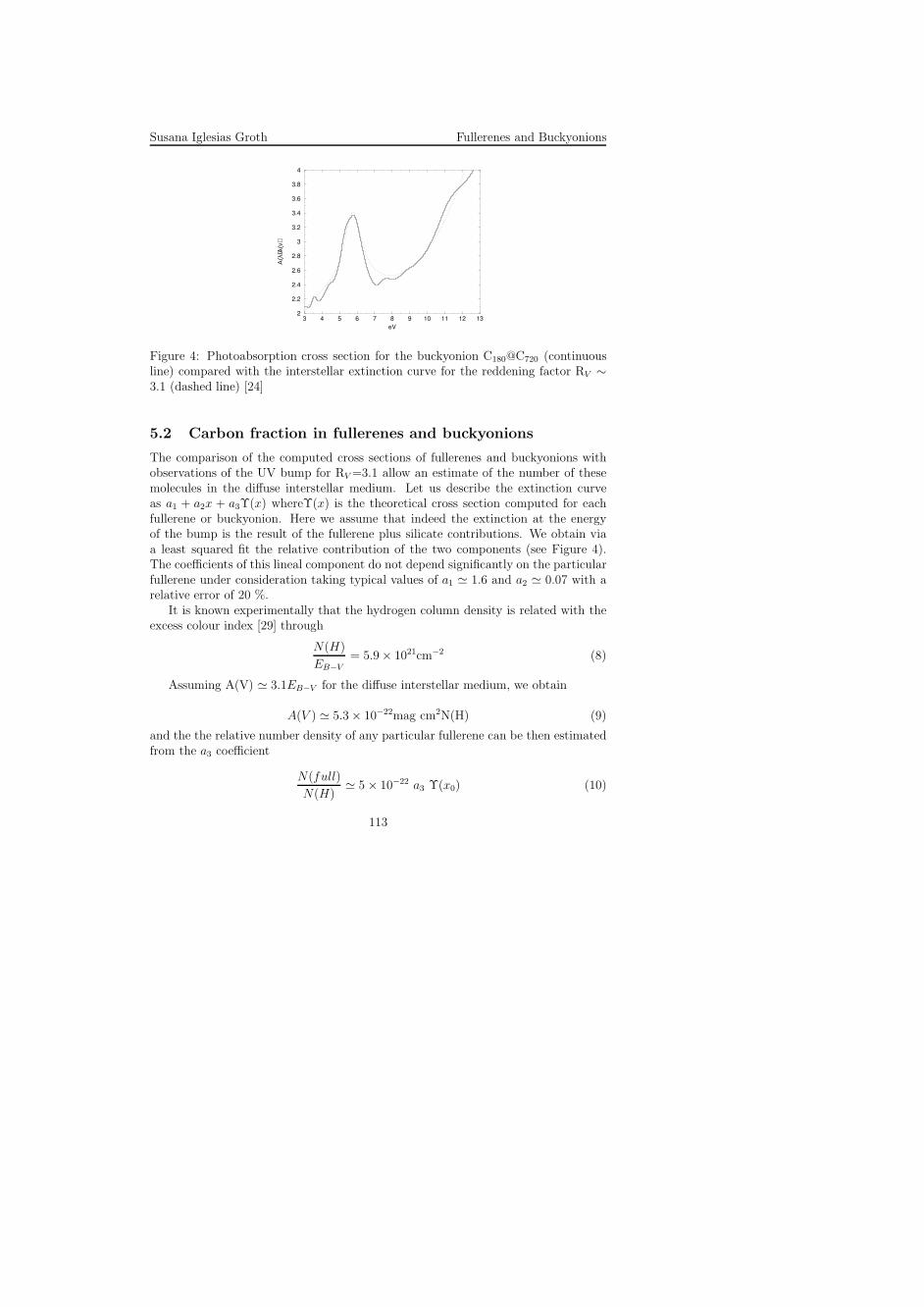
Susana Iglesias Groth Fullerenes and Buckyonions
3 4 5 6 7 8 9 10 11 12 13
eV
2
2.2
2.4
2.6
2.8
3
3.2
3.4
3.6
3.8
4
Α(λ
)/Α(ν
)
Figure 4: Photoabsorption cross section for the buckyonion C180@C720 (continuousline) compared with the interstellar extinction curve for the reddening factor RV ∼3.1 (dashed line) [24]
5.2 Carbon fraction in fullerenes and buckyonions
The comparison of the computed cross sections of fullerenes and buckyonions withobservations of the UV bump for RV =3.1 allow an estimate of the number of thesemolecules in the diffuse interstellar medium. Let us describe the extinction curveas a1 + a2x + a3Υ(x) whereΥ(x) is the theoretical cross section computed for eachfullerene or buckyonion. Here we assume that indeed the extinction at the energyof the bump is the result of the fullerene plus silicate contributions. We obtain viaa least squared fit the relative contribution of the two components (see Figure 4).The coefficients of this lineal component do not depend significantly on the particularfullerene under consideration taking typical values of a1 ≃ 1.6 and a2 ≃ 0.07 with arelative error of 20 %.
It is known experimentally that the hydrogen column density is related with theexcess colour index [29] through
N(H)
EB−V= 5.9 × 1021cm−2 (8)
Assuming A(V) ≃ 3.1EB−V for the diffuse interstellar medium, we obtain
A(V ) ≃ 5.3 × 10⁻²²mag cm2N(H) (9)
and the the relative number density of any particular fullerene can be then estimatedfrom the a3 coefficient
N(full)
N(H)≃ 5 × 10⁻²² a3 Υ(x0) (10)
113

Susana Iglesias Groth Fullerenes and Buckyonions
The typical values for a3 are of order 0.3 ×10¹⁵ (when cross sections are expressedin barns). This coefficent changes according to the type of fullerene considered butless than 50 %, corresponding to the lowest values of the largest buckyonions. Wefind then that fullerenes and buckyonions may have densities in the range 0.2-0.08particles per million (ppm) hydrogen atoms. Remarkably similar to the values foundin meteorites. In the unlikely case that all types of fullerenes considered in this studyhad the same density in interstellar space, it would require that of order 100-200atoms of carbon per 106 hydrogen atoms be locked in these molecules. This is a largefraction of the total carbon expected in the interstellar medium which we can assumeequal to the the solar atmosphere abundance of 355±50 [30]. It is also known fromobservations with the Goddard High Resolution Spectrograph of the Hubble telescopethat in interstellar space there are 140 ±20 carbon atoms per million hydrogen atomsin gaseous form [31], therefore the maximum number of carbon atoms available forfullerenes can not be larger than 200 per million hydrogen atoms.
Indeed, the actual carbon fraction in fullerenes depend of the proper mixture ofthese molecules in the interstellar medium. It is likely that the number density offullerenes and buckyonions will decrease with increasing radius (R). A distribution ofthe type N(full)∼ R−m has been frequently considered in the literature on interstellargrain populations [32]. We have studied how a mixture of fullerenes and buckyonionsfollowing such size distribution may reproduce the observed UV bump and find thatthe best fits to the shape, peak energy and width of the bump are obtained for mvalues in the range 2.5-4.5. Such values for the power-law index lead to a lower numberof carbon atoms locked in fullerenes consistent with the interstellar carbon budget.The precise determination of the actual carbon fraction requires further study andwill be the subject of a forthcoming paper.
6 Diffuse interstellar bands
We predict that fullerenes and buckyonions, contrarily to other suggested carriers forthe UV bump, display weak bands in the optical part of the spectrum. These bandspopulate with relatively high density this spectral range. Similar to what is seen inthe diffuse interstellar bands, we find for each fullerene and buckyonion a progressivedecrease of the number of transitions towards the red and infrared. Some of thesebands have wavelengths consistent with known diffuse interstellar bands, reinforc-ing the arguments for the ubiquitous presence of these molecules in the interstellarmedium.
More than 200 DIBs have been identified in the optical, most of them are foundin the range 5350- 8000 A. The stability of wavelengths and profiles suggest that thecarrier of the bands is more associated with gaseous molecules than with solid grains.The widths range between 0.8 and 30 A, thus much larger than the widths of many of
114

Susana Iglesias Groth Fullerenes and Buckyonions
the interstellar atomic lines. The bands are not significantly polarized [33]. The mostintense bands are listed in Table 1. Two DIBs at 9577 y 9632 A have been associatedto C+
60 [8] and a correlation has been claimed between the DIB at 4430 A (2.8 eV)and the UV bump [34, 35].
Wavelength(A) W(mA) Wavelength(A) W(mA)4180 0.70 6284 1.954429 3.40 6533 1.894760 0.70 6940 0.404882 0.89 7429 0.565535 0.53 8620 0.425779 0.95 9577 0.505780 0.80 9632 0.786177 2.40 13170 0.40
Table 1: The most intense diffuse bands in the interstellar medium, where W is theequivalent width [1].
In Figure 5 we plot theoretical absorption bands in the optical and near infraredobtained for individual fullerenes and buckyonions. Opposite to other molecules thathave been proposed as an explanation for the UV bump, fullerenes display a richoptical spectrum populated with relatively weak bands, of strength consistent withthose of DIBs. Almost all the fullerenes and buckyonions considered here, present astrong band at energies close to the DIB at 4430 A. We mark in Figure 5 the bandsof fullerenes and buckyonions which have a potential DIB counterpart in the list ofHerbig 1995, with a wavelength difference of less than 1%.
7 Formation of fullerenes and buckyonions
The mechanism of fullerene formation is only partially known [36]. They may beproduced at relatively high temperatures by “annealing” of large plane monocycliccarbon molecules. Buckyonions may be produced from carbon soot and from nanodi-amonds [37]. It is known that nanodiamonds of size (30-60 A) can be transformedin particles very similar to buckyonions when heated to temperatures of 1200-1800K [38] which are typical of carbon rich giant stars. The process may work as follows[37]: the (111) surfaces of nanodiamonds are the first to graphitize when treated athigh temperature, a first graphitic layer is generated on the surface and later newconcentric layers are added toward the interior in an analogous way to the process ofbuckyonion formation through energetic electron irradiation. Since diamond is moredense than graphite, the final particle has a larger size. Since the transformation takes
115

Susana Iglesias Groth Fullerenes and Buckyonions
3000 5000 7000 9000 11000 13000 15000
Longitud de onda (A)
Seccio
n e
ficaz(1
00 M
barn
)
6
6
15
20
30
40
(a)50
++ +
+
+
1500
960
720
540
240
180
60
++
+
+ ++
Figure 5: Comparation of the positions of weak bands in the theoretical spectrum ofsome fullerenes (dashed line) and buckyonions (continuous line) with known diffusebands in the interstellar medium (crosses).
place from the surface to the interior, the final particle is of spheroidal form and verycompact with the inner layer of less than 10 A of diameter. Nanodiamonds have beendetected in meteorites [39], where they are much more abundant than graphite, andpossibly in the circumstellar envelope of post-AGB stars.
References
[1] Herbig, G.H. 1995, ARA&A, 33, 19[2] Becker, L., Poreda, R.J., Bunch, T.E. 2000, Lunar and Planetary Science 31,
1803[3] Kroto, H.W. 1988, Science, 243, 1139[4] Braga, M., Larsson, S., Rosen, A., Volosov, A. 1991, A&A, 245, 232[5] Ugarte, D. 1992, Nature, 359, 707[6] Ballester, J.L., Antoniewicz, P.R., Smoluchowski, R. 1990, ApJ, 356, 507[7] Leger, A., dHendecourt, L., Verstrate, L., Schmidt, W. 1988, A&A, 203, 145[8] Foing, B.H., Ehrenfreund, P. 1994, Nature, 369, 296[9] Alasia, F., Broglia, R.A., Roman, H.E., Serra, L.L., Colo, G., Pacheco, J.M.
1994, J. Phys. B, 27, L643[10] Møller, C., Plesset, M.S. 1934, Phys. Rev., 46, 618[11] Pople, J.A., Binkley, J.S., Seeger, R. 1976, Int. J. Quant. Chem. Symp., 10, 1[12] Cioslowski, J. 1995, Electronic Structure Calculations on Fullerenes and their
Derivatives (Oxford University Press, New York)[13] Rubio, A., Alonso, J.A., Lopez, J.M., Stott, M.J. 1993, Physica B, 183, 247[14] Haddon, R.C. 1992, Accounts of Chemical Research, 25, 127
116

Susana Iglesias Groth Fullerenes and Buckyonions
[15] Lin, Y.L., Nori, F. 1996, Phys. Rev. B, 53, 1641[16] Bonin, K.D., Kresin, V.V. 1997, Electric Dipole Polarizabilities of Atom,
Molecules and Clusters, World Scientific, Singapore[17] Ruiz, A., Hernandez-Rojas, J., Breton, J., Gomez Llorente, J.M. 1998, J. Chem.
Phys., 109, 3573[18] Fanti, M., Orlandi, G., Zerbetto, F. 1995, J. Am. Chem. Soc., 117, 6101[19] Bertsch, G.F., Bulgac, A., Tomanek, D., Wang, Y. 1991, Phys. Rev. Lett., 67,
2690[20] Pariser, R., Parr, R.G. 1953, J. Chem. Phys., 21, 466; Pariser, R., Parr, R.G.
1953, J. Chem. Phys., 21, 767; Pople, J.A. 1953, Trans. Faraday Soc, 49, 1375[21] Tomanek, D., Guo, T., Jiu, C., Haufer, R.E., Chibante, L.P.F., Fure, J., Wang,
L., Alford, J.M., Smalley, R.E. 1991, J. Phys. Chem., 95, 7564[22] Yoshida, M., in http://shachi.cochem2.tutkie.tut.ac.jp/Fuller/fsl/goldberg.html.[23] Iglesias-Groth, S., Ruiz, A., Breton, J., Gomez Llorente, J.M. 2002, Journal of
Chemical Physics, 116, 1648[24] Iglesias-Groth, S. 2003, Tesis Doctoral, Universidad de La Laguna, Spain[25] Iglesias-Groth, S., Ruiz, A., Breton, J., Gomez Llorente, J.M. 2003, Journal of
Chemical Physics, 118, 7103[26] Fitzpatrick, E.L., Massa, D. 1986, ApJ, 307, 286; Fitzpatrick, E.L. 1999, PASP,
111, 63[27] Savage, B.D. 1975, ApJ, 199, 92[28] Jenniskens, P., Greenberg, J.M. 1993, A&A, 274, 439[29] Bohlin, R.C., Savage, B.D., Drake, J.F. 1978, ApJ, 224, 132[30] Grevesse, N., Noels, A. 1993, in Origin and Evolution of the Elements, ed. N.
Prantzos, E. Vangioni-Flam and M. Casse (Cambridge Univ. Press), p. 15[31] Cardelli, J.A., Meyer, D.M., Jura, M., Savage, D. 1996, ApJ, 467, 334[32] Mathis, J.S., Rumpl, W., Nordsieck, K.H. 1977, ApJ, 217, 425[33] Fahlman, G.G., Walker, G.A.H. 1975, ApJ, 200, 22[34] Nandy, K., Thompson, G.I. 1975, MNRAS, 173, 237[35] Webster, A. 1993, MNRAS, 265, 421[36] Curl, R.F., 1993 1993, Nature, 363, 14[37] Ugarte, D. 1995, ApJ, 443, L85[38] Kuznetsov, V.L., Chuvilin, A.L., Butenko, Y.V., Mal’kov, I.Y., Titov, V.M.
1994, Chem. Phys. Letters, 202, 343[39] Blake, D.F. et al. 1988, Nature, 332, 611
117

Susana Iglesias Groth Fullerenes and Buckyonions
118

COOL STARS: CHROMOSPHERIC ACTIVITY,
ROTATION, KINEMATIC AND AGE
DAVID MONTES, INES CRESPO-CHACON, M. CRUZ GALVEZ, M. JOSEFERNANDEZ-FIGUEROA, JAVIER LOPEZ-SANTIAGO, ELISA DE CASTRO,MANUEL CORNIDE, MAGDALENA HERNAN-OBISPODepartamento de Astrofısica, Facultad de Ciencias Fısicas, UniversidadComplutense de Madrid, E-28040 Madrid, SPAIN
Abstract: We summarize here our ongoing project of multiwavelength high andmedium resolution optical observations aimed at studying the chromosphere of dif-ferent kinds of late-type stars including pre-main sequence stars (weak-lined T Tauristars), chromospherically active binaries, flare stars, and young single stars membersof stellar kinematic groups. We quantify the phenomenology of chromospheric activ-ity using the information provided by several optical spectroscopic features (from theCa ii H & K to the Ca ii IRT lines) that are formed at different heights in the chro-mosphere. In addition, we obtain a better determination of the stellar parameters,spectral type, and possible binarity. With all these information we study the flux-fluxand rotation-activity relationships in order to get insights into the mechanisms whichdrive the solar-like stellar activity.
1 Introduction
Cool stars (stars with spectral type later than F2) have an outer differentially ro-tating convection zone. As in the Sun, a positive temperature gradient have beenfound in the outer atmosphere of these stars. Above the photosphere the tempera-ture increases through the chromosphere (where it reaches ≈ 104 K) and transitionregion and into the corona, where it is ≈ 106 K. This heating is thought to be dueto the dissipation of energy carried by magnetohydrodynamic waves, and/or fromreconnection of stressed magnetic field lines, but the precise physics involved is notyet understood. It is believed that convection coupled with high stellar rotation re-sults in a dynamo mechanism which converts the mechanical energy of rotation andconvection into magnetic energy. On the one hand the rotation rate in late-type starsmoderates the dynamo mechanism which generates and amplifies the magnetic fieldin the convection zone, but there is a further relationship between rotation and age.Rotation rate declines with age because stars lose angular momentum through the
119

David Montes et al. Cool Stars
coupling of magnetic field and stellar mass loss, and thus there is an indirect trendof decreasing magnetic activity with increasing age.
The stars that are rapidly rotating by virtue of their youth or presence in a close-binary system, are orders of magnitude more active than the Sun. The observations ofthese extremely active stars have revealed some very non-solar-like characteristics asconfined cool material at large distances, infalling matter, and high latitude magneticflux emergence.
Our group have been working during the last years in the analysis of high andmedium resolution spectroscopic observations that allow us to quantify the phe-nomenology of the chromospheric activity of different kinds of cool stars. We in-clude in our studies stars with different levels of activity and rotation rate, from veryyoung stars (pre-main sequence stars of weak-lined T Tauri type) to evolved starsin chromospherically active binaries (RS CVn type). Late-type stars members ofyoung stellar kinematic groups (age from 20 to 600 Myr) are being also analysed. Inaddition, we are studying the behaviour of very frequent flares and microflares thattake place in dMe dwarfs of UV Cet type (flare stars).
In the next sections we describe the methods used in our analysis, the results fromour previous studies as well as the most recent results we have obtained for all thesecool stars.
2 Observations
High and medium optical spectroscopic observations of different kinds of cool stars,covering the most of the spectral lines widely used as chromospheric activity indi-cators, have been obtained during several observing runs using different telescopesand instrumental configurations: the 2.5 m Isaac Newton Telescope (INT) with theIntermediate Dispersion Spectrograph (IDS) and the ESA-MUSICOS Echelle spectro-graph, the 4.2 m William Herschel Telescope (WHT) with the Utrecht Echelle Spec-trograph (UES), the 2.56 m Nordic Optical Telescope (NOT) using the Soviet FinishHigh Resolution Echelle Spectrograph (SOFIN) and the 3.5 m Telescopio NazionaleGalileo (TNG) using the Spectrografo di Alta Resoluzione (SARG) at the Obser-vatorio del Roque de Los Muchachos (La Palma, Spain); the 2.2 m telescope at theGerman-Spanish Observatory (CAHA) in Calar Alto (Almerıa, Spain), using a Coudespectrograph and the Fibre Optics Cassegrain Echelle Spectrograph (FOCES); the2.1 m telescope using the Sandiford Cassegrain Echelle Spectrograph and the 9.2 mHobby-Eberly Telescope (HET) with the High Resolution Spectrograph (HRS) at theMcDonald Observatory (Texas, USA). The spectral resolution achieved range from0.05 to 0.5 A.
120

David Montes et al. Cool Stars
3 Spectroscopic analysis
3.1 Chromospheric activity indicators
The simultaneous analysis of the different optical chromospheric activity indicatorsusing the spectral subtraction technique (see below), allow us to study in detail thechromosphere, discriminating between the different structures: plages, prominences,flares and microflares. The most relevant optical spectroscopic features that can beused as chromospheric activity indicators are:The Ca ii H & K lines: the emission reversals above these two strong absorptionresonance lines (see Figure 1) are the most widely used optical indicators of chromo-spheric activity, since their source functions are collisionally controlled and representan extremely important cooling mechanism.The Ca ii infrared triplet (IRT) lines: these lines share the upper levels of theCa ii H & K transitions and are formed in the lower chromosphere. The ratio of excessemission equivalent width, E8542/E8498, is an indicator of the type of chromosphericstructure (plages, prominences) that produces the observed emission.The Hα and other Balmer lines: these lines are formed at the middle chromo-sphere, but are only in emission above the continuum in very active stars, and in lessactive stars only a filled-in absorption line (see Figure 2) is observed. The EHα/EHβ
ratio can be used as a diagnostic for discriminating between the presence of plagesand prominences in the stellar surface.The Na i D1, D2 and Mg i b triplet: The Na i doublet lines are collisionallydominated and are good indicators of changes in the upper photosphere and lowerchromosphere. The Mg i b triplet lines originate in the same region. Both Na i andMg i lines are detected during flares as emission reversal or as filling-in.The He i D3 line: it originates in the upper chromosphere and the observation ofthis line in emission supports the detection of flare like events. This line could be alsofilling-in due to frequent low-level flaring activity.
The spectral subtraction technique
We determine the chromospheric contribution in these features subtracting the un-derlying photospheric contribution by using the spectral subtraction technique (see[21, 22, 23, 26, 27, 34]). This technique consists of the subtraction of a synthesizedstellar spectrum constructed from artificially rotationally broadened, radial-velocityshifted, and weighted spectra of inactive stars chosen to match the spectral types andluminosity classes of the components of the active system under consideration (seeFigs. 1, 2, 7). The synthesized spectrum is constructed using the program STARMODdeveloped at Penn State [1]. The inactive stars that we have used as reference starsin the spectral subtraction have been observed during the same observing run as theactive stars, or taken from our libraries of late-type stars (see [32]).
121

David Montes et al. Cool Stars
Figure 1: Ca ii H & K observed and subtracted spectra of the chromosphericallyactive binary VY Ari.
3.2 Radial and rotational velocities
Heliocentric radial velocities have been determined by using the cross-correlationtechnique. The spectra of the program stars were cross-correlated order by order,using the routine fxcor in IRAF, against spectra of radial velocity standards ofsimilar spectral types. We have used these heliocentric radial velocities together withprecise measurements of proper motions and parallaxes taken from Hipparcos andTycho-2 Catalogues, to calculate Galactic space-velocity components (U , V , W ) (see[35]). In the case of binary systems [12]) we have used these radial velocities todetermine the radial velocity curve and obtain a minimum χ2 fit orbit solution (seeFigure 3).
We have determined the rotational velocities (v sin i) of our star sample by usingthe cross-correlation technique. The spectrum of the program star is cross-correlatedagainst the spectrum of a template star (a slowly rotating star of similar spectraltype) and the width of the cross-correlation function is determined (see [36, 12]).The calibration of this width, to yield an estimate of v sin i, is determined by cross-correlating artificially broadened spectra of the template star for a range of v sin iwith the original template star spectrum.
3.3 Age from the Li i 6708 A line
In order to obtain an estimate of the age of our stars we have used the resonancedoublet of Li i at λ6707.8 A which is an important diagnostic of age in late-typestars, since it is destroyed easily by thermonuclear reactions in the stellar interior.The measured equivalent width of this line, EW (Li i), (corrected from the blendedFe i λ6707.41) is compared with the one of stars in well-known young open clusters
122

David Montes et al. Cool Stars
of different ages (see [36]).
4 Results
4.1 WTTS, weak-lined T Tauri stars
The weak-lined T Tauri stars (WTTS) are low mass pre-main sequence stars (PMS)with Hα equivalent widths ≤ 10 A in which no signs of accretion are observed. Theemission spectrum of these stars is not affected by the complications of star-diskinteraction which often masks the underlying absorption lines as well as extincts thestellar light in classical T Tauri stars (CTTS). The WTTS are thus ideal targets tostudy the behaviour of surface activity in the PMS stage of the stellar evolution. Alarge number of WTTS have been recently discovered by the ROSAT All-Sky Survey.Many of them have been found far away from the star formation clouds and whetherthese stars are really WTTS, or post TTS, or even young main sequence stars is amatter of ongoing debate.
We have started a high and medium resolution optical observational program ded-icated to study the chromospheric activity of late-type pre-main sequence stars. Weinclude in our study both bona-fide WTTS in Taurus with known rotational period,and WTTS recently discovered by the ROSAT All-Sky Survey, which have been verylittle studied until now. Simultaneous Hα and Ca ii H & K INT/IDS spectroscopicobservations of a sample of 20 bona-fide WTTS in Taurus-Auriga molecular clouds,with well determined photometric rotational periods, have been analysed [43, 38].The results of high resolution echelle spectroscopic observations of six ROSAT dis-covered WTTS, located in and around the Taurus-Auriga molecular clouds, can befound in [31].
4.2 Chromospherically active binaries
The chromospherically active binaries (CABS) are detached binary systems with coolcomponents characterized by strong chromospheric, transition region, and coronalactivity. The RS CVn systems have at least one cool evolved component whereasboth components of the BY Dra binaries are main sequence stars [9].
In previous work [10, 21, 22] we have studied the Ca ii H & K and Hα lines in alarge sample of CABS. The activity-rotation and flux-flux relations for these systemshave been analysed [21, 23, 24].
Multiwavelength optical observations of well known CABS
We analyzed, using the spectral subtraction technique, IDS/INT simultaneous Hα,Na i D1, D2, and He i D3 spectroscopic observations of 18 CABS [25, 26]. High
123

David Montes et al. Cool Stars
Figure 2: Spectra of 2RE J1101+223 (HD 95559) in the Hα line region. The observedspectrum (solid-line) and the synthesized spectrum (dashed-line) are plotted in theleft panel and the subtracted spectrum (dotted line) in the right panel. The positionsof the Hα line for the primary (P) and secondary (S) components are marked
resolution echelle spectra including all the optical chromospheric activity indicatorsfrom the Ca ii H & K to Ca ii IRT lines are analysed in the binary EZ Peg [27]and in other 16 CABS [34]. The subtracted Hα profile of the more active starsof the sample (Hα in emission above the continuum) has very broad wings, and iswell matched using a two-components Gaussian fit (narrow and broad). The broadcomponent is primarily responsible for the observed variations of the profile, and itscontribution to the total equivalent width (EW ) increases with the degree of activity.So we have interpreted this broad component emission as arising from microflaringactivity that take place in the chromosphere of these very active stars (see also [28]).Prominence-like extended material has been detected in a near-eclipse Hα observationof the system AR Lac. The excess emission found in the Na i D1 and D2 lines byapplication of the spectral subtraction technique, and the behaviour of the Hα linein the corresponding simultaneous observations indicate that the filling-in of the coreof these lines is a chromospheric activity indicator. In giant stars of the sample theHe i D3 line has been detected in absorption in the subtracted spectra.
124

David Montes et al. Cool Stars
Figure 3: Radial velocity data and fit vs the orbital phase of 2RE J1101+223 (HD95559). Solid symbols represent the primary and open symbols represent the sec-ondary. Squares for [17], triangles for [9], rhombus for [44], and circles and stars areour data [13]
Multiwavelength optical observations of X-ray/EUV selected CABS
As an extension of our study of well known CABS we have started to observealso CABS recently discovered by their X-ray and EUV emission detected by theROSAT satellite. We have analysed the Hα and Ca ii IRT lines of the binary system2RE J0743+224. We have found that this star, previously classified as single-linedspectroscopic binary, is a double-lined spectroscopic binary (SB2) with a K1 III pri-mary and an orbital period of 10 days. During the observations an unusual long-duration flare took place [30]. A Li i λ6708 A line enhancement was detected dur-ing the flare, which we suggest is produced by spallation reactions during the flare[29, 30]. Our observations during four observing runs from 1999 to 2001 of BK Psc(2RE J0039+103) [12] confirm the single-lined spectroscopic binary (SB1) nature ofthis system and allow us to obtain, for the first time, the orbital solution of the systemas in the case of a SB2 system. The minimum masses (Msin3i) resulting from theorbital solution are compatible with the observed K5V primary and an unseen M3Vsecondary. Both components of the binary system show high levels of chromosphericactivity. Hα emission above the continuum from both components is a persistent
125

David Montes et al. Cool Stars
feature of this system. Finally the SB2 binaries 2RE J0725-002 (V789 Mon) and2RE J1101+223 (HD 95559) [13] are analysed in detail (see the Hα emission of HD95559 in Figure 2) and an improved orbital solution has been obtained (see Figure 3).
4.3 Flare stars
Flares are events in which a large amount of energy is released in a short interval oftime, taking place changes at almost all frequencies in the electromagnetic spectrum.
The first flare ever detected was discovered in the Sun on 1 September 1859 whenCarrington [4] observed a large sunspot group looking at the solar photosphere. Sincethen, flares have been observed in many types of cool stars [42], sometimes radiatingat levels several orders of magnitude more energetic than solar flares [14]. In UV Cettype stars (late Ke or Me dwarfs) optical flares are a common phenomenon. On theother hand, flares produced by more luminous stars are usually only detected throughUV or X-ray observations. Flares from UV Cet type stars present the greatest analogyto solar flares, in contrast to other stellar sources (e.g. Algol type and RS CVn binarysystems and pre-main sequence objects) [40, 2] whose flares have probably got moredifferences than similarities with respect to the solar case. Even though flares ofUV Cet type stars present many analogies with solar flares, there are also significantdifferences, such as the amount of energy released [41]. The question is: are thesedifferences only due to the different physical conditions of the atmosphere of thesestars and the solar one, or are the environments so different that even the basic flaremechanisms may be different?
Figure 4: Flare and quiescent spectra of AD Leo, compared with the spectrum of thereference star Gl 687B (M3.5V).
126

David Montes et al. Cool Stars
Figure 5: EW(Hβ) of AD Leo versus time (JD) (MUSICOS 2001 observing run).
As in the Sun, stellar flares are believed to result from the release of free mag-netic energy stored in the corona due to reconnection of magnetic field lines [11, 16].Generally, there are two different kinds of flares [39]: confined flares, in which loopsin an active region suddenly brighten and slowly decay, and eruptive flares, in whichthe whole configuration of magnetic loops is disrupted and must be newly rebuilt.In eruptive flares the originally closed magnetic field suddenly opens, flowing plasmaupward to the corona [18]. Then, magnetic pressure begins to prevail, leading tosequential reconnections of the open field lines which create new loops. The re-connection process produces intense heating which is conducted downwards to thechromosphere and it also accelerates particles that flow along the loop. Then, thegas at the chromospheric loop footpoints is strongly heated and evaporated, makingit visible in X-rays and high-temperature lines [3]. Afterwards, the loop cools, mak-ing it visible at higher wavelengths. Meanwhile, other new loops are formed aboveit. The problem concerning the energy release and the overall spectral distributionin stellar flares has recently been discussed in view of new theoretical models andmulti-line observations, but the exact physical mechanisms involved in flares remainpoorly understood.
High spectroscopic resolution observations of different flare stars
In our previous work high resolution spectroscopic observations of several flare eventshave been analysed in different kinds of active stars. In the RS CVn systems UX Ariand II Peg flares have been detected in the Hα, Na i D1 & D2 and He i D3 lines [25, 26].A long-duration (>8 days) optical flare has been found in the recently discovered, X-ray/EUV selected, chromospherically active binary 2RE J0743+224 [29]. During thisflare we have also detected a Li i λ6708 A line enhancement probably produced by
127

David Montes et al. Cool Stars
spallation reactions during the flare. We have analysed high resolution optical echellespectra and IUE observations during a strong flare on 22 December 1993 in the veryactive, young, fast rotator, single K2 dwarf LQ Hya [33]. We have estimated the totalenergy of this flare, and discussed the broad components, asymmetries, and Dopplershifts seen in some of the emission lines. During the MUSICOS (MUlti-SIte COntinu-ous Spectroscopy) 1998 campaign we have observed almost continuously the RS CVnsystem HR 1099 for more than 3 weeks in which two flares were monitored [15].
High temporal resolution observations of Me dwarfs
The purpose of our present work is to study dMe flare stars with high temporalresolution to analyse the evolution of the observed emission lines, that are formedfrom the upper photosphere to the upper chromosphere, during the different phasesof the detected flares. Results will be used to test different flare models. We havealready studied in detail the dM3.5e flare stars AD Leo and V1054 Oph [37, 5, 6].Both stars were monitored with high temporal resolution during the MUSICOS 2001observing run (2–5 April 2001) using the Isaac Newton Telescope (INT) of the ElRoque de Los Muchachos Observatory (La Palma, Spain). We have not detectedstrong flares (see e.g. Figure 4, where the spectrum of AD Leo in the maximumof the strongest flare has been plotted in comparison to its quiescent spectrum andthe one of the reference star Gl 687B) but we have found interesting short and weakvariations with properties very similar to flares (microflares) that are produced withhigh temporal frequency (see e.g. Figure 5, where the detected flares of AD Leo havebeen identified). These flares last from 14±1 to 31±3 min in the case of AD Leo andfrom 21±2 to 96±6 min in V1054 Oph. The EW rise of the Balmer lines is larger
Figure 6: EW ratio (relative to the quiescent state) of different lines during the bestmonitored flare of AD Leo in our observations.
128

David Montes et al. Cool Stars
at shorter wavelengths (e.g. Figure 6), but their temporal evolution is quite similar.It also seems that the Ca ii H & K lines are less affected by flares, suffering a lowerincrease than the Hydrogen lines and reaching the maximum at a different time. TheBalmer lines show a red-asymmetry that becomes larger in the flare maxima (despitethe broadening of the blue wing during flares).
Figure 7: Representative spectra of PW And in the quiescent state in several chro-mospheric activity indicators.
129

David Montes et al. Cool Stars
4.4 Cool stars in young moving groups
Moving groups (MG) are kinematic coherent groups of stars [7] that could share acommon origin. In our previous work [35] we have compiled a sample of late-typestars possible members of the youngest and best documented MG: Local Associationor Pleiades moving group (20 to 150 Myr); IC 2391 supercluster (35-55 Myr); Castormoving group (200 Myr); Ursa Mayor group or Sirius supercluster (300 Myr); andHyades supercluster (600 Myr). These stars have been selected from previously es-tablished members of MG based on photometric and kinematic properties, as well asfrom new candidates based on other criteria as their level of chromospheric activity,rotation rate and lithium abundance.
In order to better establish the membership of these candidate stars in the dif-ferent young MG we have started a program of high resolution echelle spectroscopicobservations [36, 20]. The spectroscopic analysis of these stars allow us to obtain abetter determination of their radial velocity, lithium (λ6707.8 A line) EW , rotationalvelocity and level of chromospheric activity. The high resolution spectroscopic ob-servations (150 stars until now) were taken during 12 observing runs from 1999 to2002. Our results confirm the membership of several previously established members,but in other cases the kinematic and spectroscopic criteria indicate the membershipin a different MG or that the star should be considered only as a young disk starwith no clear membership in any MG. Some new spectroscopic binaries have beenidentified. The rotational modulation of the photospheric and chromospheric activityof the young, single K2-dwarf PW And (member of the Local Association) has beenanalysed in detail [19].
Acknowledgements: We would like to thank our collaborators J. Sanz-Forcada, L.W.Ramsey, B.H. Foing, D. Garcıa-Alvarez. This work was supported by the Univer-sidad Complutense de Madrid and the Spanish Ministerio de Ciencia y Tecnologıa(MCYT), Programa Nacional de Astronomıa y Astrofısica under grant AYA2001-1448. I. Crespo-Chacon would like to thank the Spanish Ministerio de Educacion,Cultura y Deporte for the PhD. grant AP2001-0475.
References
[1] Barden, S. C. 1985, ApJ, 295, 162[2] Byrne P. B. 1989, Solar Physics, 121, 61[3] Cargill P. J., Priest, E. R. 1983, ApJ, 266, 383[4] Carrington, R. C. 1859, MNRAS, 20, 13[5] Crespo-Chacon, I., Montes, D., Lopez-Santiago, J. et al. 2003, in: Highlights of
Spanish Astrophysics III, Kluwer Academic Publishers, 468[6] Crespo-Chacon, I., Montes, D., Fernandez-Figueroa, M.J., et al. 2004, Astr. &
Sp. Sc., 291, Vols 1-4
130

David Montes et al. Cool Stars
[7] Eggen, O. J. 1994, Galactic and Solar System Optical Astrometry, CambridgeUniversity Press, 191
[8] Fekel, F. C., Boop, B. W., Africano, J. L., et al. 1986, AJ, 92, 1150[9] Fekel, F. C., Gregory, W. H. 2000, ApJ, 120, 3265
[10] Fernandez-Figueroa, M.J., Montes, D., De Castro, E., Cornide, M. 1994, ApJSS,90, 433
[11] Foing, B. H. 1989, Solar Physics, 121, 117[12] Galvez, M.C., Montes, D., Fernandez-Figueroa, M.J., et al. 2002, A&A, 389, 524[13] Galvez, M.C., Montes, D., Fernandez-Figueroa, M.J., et al. 2004, A&A, in press[14] Garcıa-Alvarez, D., Jevremovic, D., Doyle, J. G., Butler, C. J. 2002, A&A, 383,
548[15] Garcıa-Alvarez, D., Foing, B., Montes, D., et al. 2003, A&A, 397, 285[16] Haisch, B., Strong, K.T., Rodono, M. 1991, ARA&A, 29, 275[17] Jeffries, R. D., Bertram, D., Spurgeon, B. R. 1995, MNRAS, 276, 397[18] Kopp, R. A., Pnewman, G. W. 1976, Solar Physics, 50, 85[19] Lopez-Santiago, J., Montes, D., Fernandez-Figueroa, M. J., Ramsey, L.W. 2003,
A&A, 411, 489[20] Lopez-Santiago, J., Montes, D., et al. 2004, A&A(in press)[21] Montes, D., Fernandez-Figueroa, M.J., De Castro, E., Cornide, M. 1995, A&A,
294, 165[22] Montes D., Fernandez-Figueroa M.J., De Castro E., Cornide, M. 1995, A&A,
109, 135[23] Montes, D., De Castro, E., Fernandez-Figueroa, M.J., Cornide M. 1995, A&ASS,
114, 287,[24] Montes, D., Fernandez-Figueroa, M.J., Cornide, M., De Castro, E. 1996, A&A,
312, 221[25] Montes, D., Sanz-Forcada, J., Fernandez-Figueroa, M.J., Lorente, R. 1996, A&A,
310, L29[26] Montes, D., Fernandez-Figueroa, M. J., de Castro, E., Sanz-Forcada J. 1997,
A&A, 125, 263[27] Montes, D., Sanz-Forcada J., Fernandez-Figueroa M.J., et al. 1998, A&A, 330,
155[28] Montes, D., Fernandez-Figueroa, M.J., De Castro, E., et al. 1998, ASP Conf.
Ser. 154, CD-1516[29] Montes, D., Ramsey, L. W., A&A, 340, L5[30] Montes, D., Ramsey, L. W. 1999, ASP Conf. Ser. , 158, p. 226[31] Montes, D., Ramsey, L. W. 1999, ASP Conf. Ser., 158, p. 302[32] Montes, D. 1999, A&ASS, 263, 275 (http://www.ucm.es/info/Astrof/spectra.html)
[33] Montes, D., Saar, S. H., Collier-Cameron, A., Unruh, Y. C. 1999, MNRAS, 305,45
[34] Montes, D., Fernandez-Figueroa, M.J., De Castro, E., et al. 2000, A&ASS, 146,103
131

David Montes et al. Cool Stars
[35] Montes, D., Lopez-Santiago, J., Galvez, M. C., et al., MNRAS, 328, 45[36] Montes, D., Lopez-Santiago, J., Fernandez-Figueroa, M. J., et al. 2001, A&A,
379, 976[37] Montes, D., Crespo-Chacon, I., Fernandez-Figueroa, M.J., et al. 2004, in: Pro-
ceedings of the IAU Symp.219 (A. Dupree & A. Benz eds.), in press[38] Montes, D., Miranda, L.F. 2004, A&A, (in preparation)[39] Pallavicini, R., Serio, S., Vaiana, G. S. 1977, ApJ, 216, 108[40] Pallavicini, R., Tagliaferri, G. 1989, in: Solar and Stellar Flares (B. M. Haisch
& M. Rodono eds.), 17[41] Pallavicini, R. 1990, IAU Symp.142, 77[42] Pettersen, B. R. 1989, Solar Physics, 121, 299[43] Poncet, A., Montes, D., et al. 1998, ASP Conf. Ser., 154, CD-1772[44] Strassmeier, K., Washuettl, A., Granzer, T., et al. 2000, A&ASS, 142, 275
132

ASTEROSEISMOLOGY OF HOT SUBDWARF
STARS
RAQUEL OREIRO REYInstituto de Astrofısica de Canarias, E-38200 La Laguna, SPAINDepartamento de Astrofısica, Universidad de La Laguna, E-38200 La Laguna,SPAINCRISTINA RODRıGUEZ LOPEZ, ANA ULLADepartamento de Fısica Aplicada, Universidade de Vigo, E-36200 Vigo, SPAINFERNANDO PEREZ HERNANDEZInstituto de Astrofısica de Canarias, E-38200 La Laguna, SPAINDepartamento de Astrofısica, Universidad de La Laguna, E-38200 La Laguna,SPAINRAFAEL GARRIDOInstituto de Astrofısica de Andalucıa-CSIC, E-18008 Granada, SPAINMINIA MANTEIGADepartamento de Ciencias de la Navegacion y de la Tierra, Universidade daCoruna, E-15011 A Coruna, SPAINJAMES MACDONALDDepartment of Physics and Astronomy, University of Delaware, Newark, DE 19716,USA
Abstract: We present a summary of the current state of the art in the study ofhot subdwarf stars by using asteroseismological techniques. We first briefly describethe main physical aspects of these objects, to then analyze the different groups of hotsubdwarfs from a seismological point of view.
1 Introduction
Since 1947, when Humason & Zwicky discovered hot subdwarfs on a survey of faintblue stars [1], and from 1960, when Greenstein established them as a spectroscopi-cally diferentiated class of stars [2], they had been scarcely studied by the scientificcommunity. A situation that reversed after the discovery of pulsations in some hotsubdwarfs stars in 1997 [3].
This class of objects consists mainly of subluminous stars with a canonical mass of0.5M⊙; they have blue colors and effective temperature ( Teff ) and logarithm of surface
133

Raquel Oreiro Rey et al. Asteroseismology of Hot Subdwarfs
gravity (log g) in the ranges 20 000 – 100 000 K and 4.0 – 6.5 dex, respectively. Hotsubdwarfs reveal themselves as abundant objects in faint and blue stellar surveys [4].Due to their high temperatures they have been considered as ionizing sources ofinterstellar gas at high galactic latitudes [5], and they are thought to be responsiblefor the UV-upturn found in elliptical galaxies and galaxy bulges [6], [7], [8].
Their evolutionary status corresponds to a lower main sequence star that hasevolved through the Red Giant Branch, but that has not yet arrived at the coolingsequence of White Dwarfs (WDs). The specific details of their evolution, as well asother aspects –such as the population they belong to (they are found both in thedisk and the galactic halo [9], their anomalies in metal abundances [10], their binaryfraction, and the nature of the detected oscillations– are still a matter of investigation.
A definite spectroscopic classification has not yet been established either, despitevarious existing proposals [11], [12]. However, we can segregate hot subdwarfs intothree main spectroscopic sequences, sdBs, sdOs and sdOBs, according to compositionand effective temperatures:
• sdBs have hydrogen dominated atmospheres, with Teff between 20 000 and 40 000K, and log g between 5.2 and 6.5 dex.
• sdOs have helium rich atmospheres, with Teff between about 40 000 K and100 000K and log g between 4.0 and 6.5 dex.
• sdOBs share characteristics of the above types, both hydrogen and helium arepresent in their atmospheres and they have Teff around 40 000K.
2 Subdwarf B-Type Stars
The physical parameters specified in the previous section place subdwarf B-type stars(the sdBs) in the area of the Hertzsprung Russell Diagram (HRD) known as theExtended Horizontal Branch ([15], EHB) a region that corresponds to the bluest partof the Horizontal Branch. This location is reproduced by theoretical models of He-core burning stars having q ∼ 0.95, where q=Mcore/Mtotal [13], [14]. They also havea radiative He-layer plus a small (MH ≃ 0.02M⊙) and inert hydrogen envelope, thatmakes the model behave almost like a helium Main Sequence star [15], [16].
Although their evolutionary path is not yet compleltely understood, they arethought to be descendents of Red Giant Branch (RGB) stars that have undergonesuch substantial mass loss that they have lost most of their H envelope and bypass theAsymptotic Giant Branch evolving directly into the White Dwarf cooling sequence.However, the exact mechanism that produces such mass loss at or near the tip of theRGB is unclear. Because at least 44% of the sdBs show signs of binarity, a binaryorigin involving common envelope phases has also been proposed [17]. Some binaryscenarios of sdB formation have been studied [18] from a theoretical point of view.
134

Raquel Oreiro Rey et al. Asteroseismology of Hot Subdwarfs
Subdwarf-B stars are all chemically peculiar, with spectra dominated by theBalmer lines; they show an underabundance of He that can be very noticeable insome particular cases [19]. Other elements, such as C and Si, appear depleted intheir spectra while N is aproximatly solar. The chemical abundances could resultfrom the balance between gravity and radiative levitation, but this does not seemto be the case: the radiative and gravitatory mechanisms alone can not explain theobservations [10]. Other mechanisms such as mass loss, rotation or magnetic fields,have been proposed in the attempt of reproducing observed sdB spectra [20], [21].
2.1 Pulsations in sdBs
The discovery of pulsations in some of the sdBs allows us to improve our knowledgeof these stars interior structure by making use of asteroseismological techniques.
The first pulsating sdB, EC14026-2647, was found in 1997 [3]. Several obser-vational campaigns were then organized to search for similar objects. The intensesearches performed by the South African Astronomical Observatory ([22] and refer-ences therein), University of Montreal [23], Nordic Optical Telescope [24] and recently,by Green and collaborators [25], established two subclasses of pulsating sdBs. Theydisplay the following differences:
• The objects in the “EC14026” subclass have fast pulsations, with periods thattend to cluster in the range (80-250) s. There exist, however, some particularcases (Feige 48, HS 2201+2610, HS 0702+6043 and PG1605+072) with longerperiods (up to 600 s) that are explained by a frequency dependence on thephysical parameters of the star [26]. The detected frequencies are explained asp modes, both radial and non radial, of low degree and low radial order excitedby the κ mechanism associated with an opacity bump due to the enhancementof the iron abundance in the sdB envelopes, probably caused by diffusion pro-cesses [27]. The Teff and log g of EC14026 stars, between 28 400 – 35 700 K and5.25 – 6.11 dex, respectively, place them in an area of the HRD where theycoexist with constant sdBs. To date, it remains unknown what causes somestars to pulse while others, with the same physical parameters, do not. Theexplanation could involve weak winds that, at differents ages, would lead todifferences in the amount of iron in the pulsation driving region [28].
• The subclass know as “Betsy” stars, discovered in 2002 [25], show periods ofoscillation on the order of one hour, that are attributed to g modes of highradial order excited by the same mechanism acting in the EC14026 stars. Wefind Betsy stars in the HRD area enclosed by the values of Teff ∈ [25 000, 30 000]K and log g ∈ [5.4, 5.7], respectively. In this case, it seems that all the stars lying
135

Raquel Oreiro Rey et al. Asteroseismology of Hot Subdwarfs
in this region oscillate and there is no co-existence of pulsating and constantobjects.
Figure 1: Some typical light curves of EC14026 (top) and Betsy stars (bottom) [29].
In Figure 1 some typical light curves of the two subclasses of pulsating sdBs areshown.
The observational discovery of the first pulsating sdB almost coincided with thetheoretical prediction of the viable existence of pulsations in this class of stars. Mo-tivated by the presence of a HeII-HeIII convection zone in the sdB envelopes thatcould excite pulsation modes, Charpinet et al. made the first theoretical study of thepossible oscillating nature of sdBs [30]. Contrary to their expectations, they found anegligible contribution to driving from the HeII-HeIII region but an important con-tribution due to ionization of heavy elements. The same authors obtained excitedpulsation modes in sdB models with enhanced Fe abundances [27]. They establishedthat sdB models with an inhomogeneous iron distribution could present excited modesif enough of this element were present in the driving region, and proposed that the
136

Raquel Oreiro Rey et al. Asteroseismology of Hot Subdwarfs
iron opacity κ mechanism is responsible for pulsations in EC14026 stars. The studiesabove mentioned formed the basis for an asteroseismological study of sdBs.
Fontaine et al. provided a theoretical explanation for the occurrence of oscillationsin the Betsy stars [29]. The same κ mechanism that excites p modes in EC14026 starsis proposed as responsible for the light curve variations on Betsy stars, but leadingto excited g modes of high radial order in this case.
The discovery of an oscillatory behaviour for some sdBs has led to investing greateffort in trying to remove some of their uncertainties but, above all, it has opened thepossibility of using seismological techniques to probe their interiors and, hence, togain more information about this still puzzling stellar evolutionary phase. However,this task is not lacking of problems: the low number of detected pulsation frequen-cies in some cases, the complexity of the amplitude spectra in others, and the lowamplitudes of pulsation, of the order of a few milli-magnitudes, that prevent us fromaccurate mode identifications, are delaying the application of seismology techniquesto studying sdBs in detail. In the near future, with the aid of space missions, likeCOROT [31], these problems may be overcome, but to date, the only existing com-plete asteroseismological analysis of a sdB can be found in [32] and [33].On this scene, our group is working both observationally and theoretically. Theuse of the IAC80 telescope (Teide Observatory) has led to the discovery of thelatest EC14026 star known to date: Balloon090100001 [34], which is the brightest(B = 11.8) and has one of the greatest pulsation amplitudes (∼ 60 mmag) amongits class. On the other hand, we are able to compute full stellar evolution structuralmodels of sdB stars by using the code of one of us (JM, [35]), and their correspond-ing theoretical frequencies of pulsation by using the adiabatic code of Christensen-Dalsgaard [36]. These computational results are used to carry out the seismologicalanalysis of the observational data.
3 Subdwarf O-Type Stars
Hot subdwarfs O-type (hereafter sdOs) are helium rich objects with a mean canonicalmass of M = 0.5M⊙. They most likely have C/O cores with a helium burningshell. Their exact evolutionary state is still uncertain, in part due to a paucity ofstellar evolution calculations for these objects. Nevertheless, two possible scenariosexplaining the origin of sdOs have been proposed based on their location in the HRdiagram [37]:
• The post-AGB (Asymptotic Giant Branch) or “luminous” sdOs are found in aregion of the HRD crossed by tracks leaving the AGB.
• The post-EHB (Extended Horizontal Branch) or “compact” sdOs sit on theHRD near the EHB region. The majority of sdOs are found in this location.
137

Raquel Oreiro Rey et al. Asteroseismology of Hot Subdwarfs
Both of these scenarios pose a number of yet unanswered questions:The “luminous” sdOs would be the descendants of AGB objects and would evolve
like central stars of planetary nebulae. However, only four sdOs are known that showsigns of a surrounding nebula [38], [39]. Some explanations to why this is have beenproposed by [40] and [42].
The “compact” sdOs would be the sdBs (EHB) descendants. The main questionis how a hydrogen rich star (a sdB) may have evolved into a helium rich one (a sdO).There are only a few calculated tracks for the post-HB state (see [13], [43], [44], [45]and [46]). Recently, Lanz et al. have used “deep helium flash-mixed models” toaccount for helium enriched sdBs [47]. Their models yield effective temperatures onthe Zero Age Horizontal Branch higher than the canonical value which may explainthe helium enrichment and give subsequent evolution to the sdOs.
A binary origin of sdOs has been addressed in [41] and [48]. It is proposed thatsingle sdOs may be the merger of a pair of low-mass helium WDs which lose angularmomentum by gravitational wave radiation. There are a few studies which estimatethe binary fraction of sdOs ( [17], [49], [50], [51] and [52]) at between 30 and ∼64%.
The highly inhomogeneous sdOs spectra (with the common characteristic of ausually strong HeIIλ4686A spectral line) echo the peculiarities of their atmospheres.There are to date few exhaustive spectral analyses of sdOs (see e.g.: [53], [54], [55]).From them, we know that the helium abundance (from 50% to a 100%) shown intheir spectra is usually accompanied by nitrogen enhancement and carbon depletion,pointing to the action of the CNO cycle, while sometimes carbon is enhanced whichshows the action of the 3α process. Enhancement and depletion, in various degrees,of other metals like oxygen, silicon, magnesium, neon and iron in different stages ofionization are also found [56], rendering the spectral classification into subclasses ofthese objects still a matter of debate [12].
3.1 Search for pulsations in sdOs
Tracing back the history of pulsations in sdOs, as early as 1957 (only ten years afterthe discovery of hot subdwarfs ) J. L. Greenstein in his paper “Evidence for instabilityamong sub-luminous stars” [57] recommended observations to detect possible short-period pulsations among sdOs and WDs.
Bartolini et al. were the next to consider variability among sdOs [58]. They carriedout a photometric study searching for variability in 6 hydrogen-poor stars, 3 of thembeing sdOs. They claimed to have found microvariability in all of them, althoughthey were only able to estimate periodicities qualitatively.
The same authors stated the pulsational behavior of a binary system composedof the sdO star HD128220 and a subgiant type-G companion [59]. However, it wasnot clear if the observed small amplitude variations were due to the sdO star or to itscompanion, or to fluctuations in atmospheric transparency [60]. Some non-pulsating
138

Raquel Oreiro Rey et al. Asteroseismology of Hot Subdwarfs
episodes in the system, attributed to destructive interference of nearby frequencies,were also reported.
Motivated by the exciting discovery of pulsations in sdBs, and taking into con-sideration the related studies above [59], we have begun a photometric study of asample of about 60 sdOs. Our objective is to search for possible pulsations amongthem, with the final aim of shedding some light on their evolutionary state.
11 sdOs and one sdOB have been observed in three observational campaigns: oneat the Sierra Nevada Observatory (OSN) in December 1999, where 4 channel simul-taneous Stromgren photoelectric photometry was performed with a 90 cm telescope,and two in April and August-September 2003 at the IAC80 telescope (Teide Ob-servatory; OT) where fast photoelectric photometry was made with the 3 channelTromsø-Texas photometer in white light. On the latter occasion, B Johnson CCDphotometry was also acquired with the Tromsø-Texas CCD photometer.
From our spectral analysis, the star HIP 52181 stands out with a frequency of1,04 mHz and with an amplitude over 2,5σ times the mean noise, which makes it agood candidate for pulsations. The amplitude spectrum is plotted in Figure 2. Thehorizontal dotted line is 2,5σ times the mean value of the amplitude, and the solidline is 3 times this value which yields roughly a 99% confidence level.
Figure 2: Amplitud spectra for HIP 52181.
For this candidate star a preliminary asteroseismological study was implemented.Two sdO models with atmospheric parameters roughly reproducing those of HIP 52181,were computed with the stellar evolution code of JM [35] by evolving Z=0.02, 1.0M⊙
stars from the main sequence with enhanced mass loss. These were then used as in-put to the stellar evolution code to produce 19 more evolved structural models. The
139

Raquel Oreiro Rey et al. Asteroseismology of Hot Subdwarfs
evolution was stopped at log g∼7, when the star is entering the WD phase. The twoevolutionary tracks are plotted in the HRD (Figure 3).
Figure 3: Traks in the HRD computed after evolving two sdOs structural models tothe WDs phase.
We chose the 7 models marked with diamonds on Figure 3 and used them asinput for the adiabatic pulsation code of Christensen-Dalsgaard [36]. Only for oneof the models were two theoretical frequencies obtained that consistent with our ob-servational data. Both frequencies are identified with high order g modes. Furtherobservational and theoretical work is required to asses the eventual meaning of thesepreliminary results. In particular, one of our immediate goals is to construct moreaccurate structural models of sdOs and to use them with a non-adiabatic pulsationcode [61] that includes the interaction between pulsation and the atmosphere to de-termine the unstable oscillation modes.
About 20 more sdOs of the ongoing study were observed from 1-14 December 2003at OSN with a 1.5 m telescope with a B Johnson filter. The data obtained are underanalysis. If the pulsating/non-pulsating rate is similar to that found for the sdBs, atleast 1 or 2 new sdO pulsators are expected on the completion of the photometricstudy.
Acknowledgements: Part of this work was supported by MCyT under project AYA2000-1691. R. Oreiro acknowledges CajaCanarias and C. Rodrıguez Lopez Xunta de Galiciafor its financial support. We thank the Centro de Supercomputacion de Galicia forthe use made of their computational facilities.
140

Raquel Oreiro Rey et al. Asteroseismology of Hot Subdwarfs
References
[1] Humason, M.L., Zwicky, F. 1947, ApJ, 105, 85[2] Greenstein, J.L. 1960 in Stellar atmospheres, University of Chicago Press[3] Kilkenny, D., Koen, C., O’Donoghue, D., Stobie, R. S. 1997, MNRAS, 285, 640[4] Green, R. F., Schmidt, M., Liebert, J. 1986, ApJSS, 61, 305[5] de Boer, K.S. 1985, A&A, 142, 321[6] Bica, E., Bonatto, C., Pastoriza, M. G., Alloin, D. 1996, A&A, 313, 405[7] Brown, T. M., Ferguson, H. C., Davidsen, A. F., Dorman, B. 1997, ApJ, 482,
685[8] Yi, S. 1997, Bull. of the American Astron. Soc., 29, 1407, 19112402[9] Colin, J., et al. 1994, A&A, 287, 38
[10] Michaud, G., Bergeron, P., Wesemael, F., Fontaine, G. 1985, ApJ, 299, 741[11] Moehler, S., Ritchtler, T., de Boer, K.S., Dettmar, R.J., Heber, U. 1990,
A&A Sup. Ser., 86, 53[12] Jeffery, C.S., Drilling, J.S., Harrison, P.M., Heber, U., Moehler, S. 1997,
A&A Sup. Ser., 125, 501[13] Dorman, B., Rood, R.T., O’Connell, R.W. 1993, ApJ, 419, 596[14] Oreiro, R., Ulla, A., Perez Hernandez, F., MacDonald, J., Garcıa, R., Zapatero,
M.R. 2004, in preparation[15] Heber, U. 1986, A&A, 155, 33[16] Saffer, R., Bergeron, P., Koester, D., Liebert, J. 1994, ApJ, 432, 351[17] Ulla, A., Thejll, P. 1998, A&A Sup. Ser., 132, 1[18] Han, Z., Podsiadlowski, Ph., Maxted, P.F.L., Marsh, T.R., Ivanova, N. 2002,
MNRAS, 336, 449[19] Heber, U., Reid, I.N., Werner, K. 2000, A&A, 363, 198[20] Unglaub, K., Bues, I. 1998, A&A, 338, 75[21] Elkin, V.G. 1996, A&A, 312, L5[22] Koen, C., O’Donoghue, D., Kilkenny, D., Stobie, R. S., Saffer, R. A. 1999, MN-
RAS, 306, 213[23] Billeres, M., Fontaine, G., Brassard, P., Liebert, J. 2002, ApJ, 578, 515[24] Oestensen, R., Solheim, J.-E., Heber, U., Silvotti, R., Dreizler, S., Edelmann, H.
2001, A&A, 368, 175[25] Green, E. et al. 2003, ApJ, 583, L31[26] Charpinet, S., Fontaine, G., Brassard, P., Dorman, B. 2002, ApJSS, 139, 487[27] Charpinet, S., Fontaine, G., Brassard, P., Chayer, P., Rogers, F. J., Iglesias, C.
A., Dorman, B. 1997, ApJ, 483, L123[28] Chayer, P. 2003, ApJSS, in press[29] Fontaine, G., Brassard, P., Charpinet, S., Green, E. M., Chayer, P., Billres, M.,
Randall, S. K. 2003, ApJ, 597, 518[30] Charpinet, S., Fontaine, G., Brassard, P., Dorman, B. 1996, ApJ, 471, 103[31] Baglin, A., Vauclair, G. & The COROT team 2000, JApA, 21, 319
141

Raquel Oreiro Rey et al. Asteroseismology of Hot Subdwarfs
[32] Brassard, P., Fontaine, G., Billeres, M., Charpinet, S., Liebert, J., Saffer, R. A.2001, ApJ, 563, 1013
[33] Charpinet, S., Fontaine, G., Brassard, P. 2001, ASP, 113, 775[34] Oreiro, R., Ulla, A., Perez Hernandez, F., Oestensen, R., Rodrıguez Lopez, C.,
MacDonald, J. 2004, ApJ, accepted[35] Jimenez, R., MacDonald, J. 1996, MNRAS, 283, 721[36] Christensen-Dalsgaard, J., Berthomieu, G. 1991, Solar interiors and atmo-
spheres, ed., A: N: Cox, W. C. Livingston & M. Mathews (Univ. Arizona Press),401
[37] Husfeld, D. 1987, Proc. of the 2nd Conference on Faint Blue Stars , Schenectady,NY, L. Davis Press, p.237
[38] Pritchet, C. 1984, A&A, 139, 230[39] Kwitter, K. B., Congdon, C. W., Pasachoff, J. M., Massey, P. 1989, AJ, 97, 1423[40] Schonberner, D. 1983, ApJ, 272, 708[41] Iben, I. Jr., Tutukov, A.V. 1986, ApJ, 311, 753[42] Brocato, E., Matteuci, F., Mazzitelli, I., Tornambe, A. 1990, ApJ, 349, 458[43] Sweigart, A. V., Mengel, J. G., Demarque, P. 1974, A&A, 30, 13[44] Gingold, R. A. 1976, ApJ, 204, 116[45] Caloi, V., 1989, A&A, 221, 27[46] MacDonald, J., Arrieta, S. 1994 Hot Stars in the Galactic Halo, Cambridge
University Press, p. 238[47] Lanz, T., Brown, T. M., Sweigart, A. V., Hubeny, I., Landsman, W. B. 2004,
ApJ, 602, 342[48] Webbink, R. F. 1984, ApJ, 277, 355[49] Thejll, P., Ulla, A., MacDonald, J. 1995, A&A, 303, 773[50] Williams, T., McGraw, J.T., Grashuis, R. 2001, PASP, 113, 490[51] Williams, T., McGraw, J.T. 2001, PASP, 113, 94[52] Stark, M. A., Wade R. A. 2003, ApJ, 126, 1455[53] Dreizler, S., Heber, U., Werner, K., Moehler, S., de Boer, K. S. 1990, A&A, 235,
234[54] Thejll, P., Bauer, F., Saffer, R. et al 1994, ApJ, 433, 819[55] Bauer, F., Husfeld, D. 1995, A&A, 300, 481[56] Heber, U. 1998, Proc. of the conference UV Astrophysics. Beyond the IUE Final
Archive’, ESA, SP-413[57] Greenstein, J.L. 1957, Proc. of the 4th IAU Sym., Cambridge University Press,
p. 179[58] Bartolini, C., Bonifazi, A., D’Antona, F. et al. 1982, ApJSS, 83, 287[59] Bartolini, C., Bernabei, S., Bruni, I. et al. 2001, Mem.S.A.It, 72, 4[60] Piccioni, A., Bartolini, C., Bernabei, S. et al. 2002, Proc. of the 1st Eddington
Workshop, ESA SP-485, p. 305[61] Moya, A., Garrido, R., Dupret, M. A. 2004, A&A, 414, 1081
142

HELIUM CATACLYSMIC VARIABLES
RICARDO MORENO, ANA ULLADepartamento de Fısica Aplicada, Universidade de Vigo, E-36200 Vigo, SPAIN
Abstract: The so-called AM CVn systems, or Interacting Binary DB WhiteDwarf stars, have grown from four members in 1992 to twelve in 2003; five out ofthe eight new discoveries were found during the 21st century. Also, the observationalproperties of these systems show nowadays a widespread and unexpected range ofcharacteristics, which seems to confirm the existence of “subclasses” within the group.Four objects at least show X-ray emission. For two objects at least, H seems to havebeen detected in their optical spectra. A brief review of the recent findings for thispeculiar group among the Cataclysmic Variables is here presented.
1 Introduction
A Cataclysmic Variable (CV) is, by its usual definition, a close interacting binary sys-tem where a solar-type secondary star overflows its Roche Lobe and donates matter,mostly hydrogen from its atmosphere, in a stable manner onto a White Dwarf (WD)primary accretor, within orbital time spans in the range of hours. Excellent reviewson the topic can be found in, e.g., [1], [2], [3], [4].
Helium Cataclysmic Variables (He CVs), also referred to as AM CVn systems ([5],[6]) or Interacting Binary DB White Dwarf stars (IBDBWDs: [7], [8], [9]), constitutea subclass of the CVs where the secondary star is a Helium-rich WD (i.e., of DBtype), donating matter onto the primary object, which is also a DB WD. Two maincharacteristics distinguish them from the bulk of the H-rich CVs: their composition(with spectra entirely depleted from H and dominated by He lines) and their ultra-short orbital periods (on the order of minutes). See for example [10], [5], [9], [11], fora revision of their properties.
Until 1992 only four AM CVn objects were known (AM CVn, V803 Cen, CRBoo and GP Com), despite the prototype, AM CVn itself, had been discovered asa variable object by [12] and classified as an IBDBWD system by [13]. A review oftheir characteristics published to that date can be found in [9]. Tables listing thetwelve AM CVn systems known to date, together with a summary of some of theirproperties, can be found in, e.g., [14].
In the next sections, some of the main recent findings for the objects will besummarized, together with a discussion of their implications in the context of theCataclysmic Variables.
143

Ricardo Moreno and Ana Ulla Helium Cataclysmic Variables
2 The objects
There are at present twelve AM CVn systems identified and catalogued as such,namely AM CVn, HP Lib, GP Com, CE 315, V803 Cen, CR Boo, CP Eri, KLDra, 2003aw, V407 Vul, ES Cet and RX J0806.3+1527 (RX J0806, hereafter), which,according to [14] could be grouped into three classes: the “high state” objects AMCVn and HP Lib, with orbital periods shorter than 1200 seconds, a high mass transferaccretion rate and a thick disk, showing absorption He lines in their optical spectra;the “low state” objects GP Com and CE 315, with orbital periods larger than 2500seconds, a low mass transfer accretion rate and a thin disk, showing emission lines; andthose objects in an “unstable (or cyclic) state”, with periods ranging from about 1200to 2500 seconds and showing both He emission (when in low state) and absorption(when in high state) lines. These would be V803 Cen, CR Boo, CP Eri, KL Draand 2003aw.
It is worth noting that already in 1992 V803 Cen and CR Boo were considered“intermediate” objects between AM CVn (assumed in a permanent high state) andGP Com (in a permanent low state), according to the variations of their observedmagnitudes: V ∼ 14 for AM CVn, V ∼ 16 for GP Com, and V between ∼13 and 18for V803 Cen and CR Boo ([9]). So, we see that nowadays more systems have beenfound to fit within the three classes.
On the other hand, V407 Vul and RX J0806 are found to display X-ray emission([15], [16]) while [17] suspected ES Cet to be a soft X-ray source. The three systemshave been proposed to host magnetic primaries ([18], [17]). They display periodsranging from 321.5 to 620.26 seconds; periods that would place them inside the “highstate” regime of the AM CVn systems as previously defined. However, while V407Vul does not display emission lines and only a dubious Mg I absorption line wasdetected in its optical spectrum ([19]), ES Cet and RX J0806 only display emissionlines of He ([17], [20]), a characteristic of the “low state” objects. Besides, [21], [22]claim the detection of Balmer lines in the optical spectra of ES Cet and RX J0806,respectively, disregarding therefore their classification as AM CVn systems. All thesepeculiarities render the three objects as most peculiar and worth studying ones.
In what follows, a brief summary of characteristics and findings –which does notmean to be complete, will be included for each of the twelve AM CVn systems.
2.1 “High state” objects:
AM CVn: Until 1999 two main photometric periods, ∼1051 and ∼1028 seconds,coexisted for the prototype of the IBDBWD stars group, when [23] confirmed thatthe orbital period was 1028.73 seconds, a value also later on confirmed by [24]. [25] and[26] supported the interpretation of 1051 seconds as the “superhump” period for the
144

Ricardo Moreno and Ana Ulla Helium Cataclysmic Variables
system. These two findings were crucial for a significant advance in the understandingof the binary nature of AM CVn, which, for several authors had not even been provenbeyond doubt before (see, e.g., [9]).
To date, after several disk models have been proposed for the system (e.g., [5], [27],[28], [29], [25], [24]), an accretion rate of 1014 kg/s, a precession period of 13.38 hoursand an inclination of about ∼15–45, are suggested. Also, the masses for the primaryand secondary components would be, respectively, 0.84 and 0.07 M⊙, yielding a massratio (q) of 0.087 ([25]). Instead, [30] reports values of 0.5 M⊙ and 0.22 for theprimary mass and q, respectively.
HP Lib : EC15330-1403, also known as HP Lib ([31]), was discovered as anAM CVn system by [32]. The object did not display magnitude variations withinseveral days, staying around a magnitude of V=13.6. A value of 1102.7 seconds wasassigned to its orbital period ([31]). Only HeI absorption lines were found in its opticalspectrum, with no traces of H. The system is though to remain in a permanent highstate, as AM CVn itself, and a period of 1119 seconds ([32]) has been identified asthe the superhump period of the object ([31]).
2.2 “Low state” objects:
GP Com: When only five AM CVn systems were known, around 1993, GP Comwas suggested to be the most different object among them, based on its observationalcharacteristics ([33], [34], [35]). A most intriguing feature was a variable “centralspike” displayed by its tripple-peaked emission lines of He, of unknown origin. Nowa-days, it seems well established that GP Com is an AM CVn system, with an orbitalperiod of 2794 seconds, a mass ratio on the order of 0.02 and a primary mass around1 M⊙ ([36]). [37] reported that observed flares in its light curve are generated atthe inner disk , which is thin, in a permanent (quiescent) low state and with a lowmass transfer rate ([27], [25]). As a major discovery for GP Com, the origin of its“central spike” is found to be very close to the accreating primary WD, and it is dueto Stark effect ([37]). X-ray emission has been reported for the system ([38], [39],[40], [35], [41]).
CE 315: It was discovered spectroscopically by [42], who reported the presenceof HeI and HeII lines and no traces of H, and classified it as an AM CVn system. Theoptical spectrum of the target was found to resemble very closely that of GP Com,with tripple-peaked emission lines –as stated, its most peculiar and unique featureamong the AM CVn’s, with the central spike variable. The orbital period reported bythe authors, of 3906 seconds, is the largest one found to date for an AM CVn system.They also suggested values of 0.77 and 0.017 M⊙ for the masses of the primary andsecondary component, respectively, and a mass ratio q of 0.022. [43] detected the
145

Ricardo Moreno and Ana Ulla Helium Cataclysmic Variables
existence of CNO material in CE 315, according to their spectroscopical analises, acharacteristic also shared by GP Com ([44]).
2.3 “Cyclic state” objects:
V803 Cen: Like several other AM CVn systems, V803 Cen has a thermally unstabledisk ([27], [45]), where a variable mass transfer rate makes the system oscillate amonga high (V ∼ 13), a low (V ∼ 17) and a “cyclical” (V ∼ 13.5 - 14.5 for more than 50%of the time) states ([46]). Its optical spectrum shows HeI lines ([47], [48]), both inemission (when at low state) and in absorption (when at high state).
[46] have suggested that the system undergoes normal outbursts, like the DwarfNovae ([45]), a possibility already pointed out by [49]. A period of 1618 secondsdisplayed by the object was suggested by the authors to be attributable to its super-humps; a possibility confirmed by [45] who reported values of 1614.5 and 1618.1 sec-onds for its superhump period and “late” superhumps, repectively. [45] also reporteda value of 1594 seconds for the orbital period of V803 Cen, although no conclussivelyresults exist for that issue so far.
[50] reported a low X-ray count rate detection for the system, compatible with a10 keV bremsstrahlung source.
CR Boo: PG1346+082, also known as CR Boo, shares many observational prop-erties with V803 Cen. In this case, several precession periods for its small disk([27], [51]) have been suggested: 1.18 days by [52]; 36 hours by [51]; and 32 hours by[25]. Superhumps have been observed when in high state with a superhump period of1487.29 seconds, while its orbital period seems to be established around 1471 seconds([51]). [52] also compared de object with a Dwarf Nova and provided the followingvalues for its q and secondary mass: 0.057 and 0.057 M⊙, respectively. [25] gave avalue of 43.8 for the disk inclination angle and values of 0.05 and 0.05 M⊙ for q andthe secondary mass, respectively. Meanwhile, [27] assigned to the secondary mass avalue of 0.14 M⊙.
CP Eri: [53] classified CP Eri as an IBDBWD star, of similar characteristics tothose of V803 Cen and CR Boo. They found a period of 1724 seconds, no H in itsoptical spectrum, and a transition between emission and absorption of its He linesfrom low (at a V magnitude of ∼ 19.7) to high (V magnitude of ∼ 16.5; see [53]for details), respectively, of its thermally unstable disk ([25], [27]). A clear orbitalnature for that dominant period has not been established yet, as far as we can tell.[54] reported double-peaked lines of He I in emission, similar to those found for GPCom and CE 315, together with emission lines of Si II. The authors also reported aprimary mass of at least 0.27 M⊙ and an inclination angle for the disk in the range33–80.
146

Ricardo Moreno and Ana Ulla Helium Cataclysmic Variables
KL Dra: KL Dra ([55]) was discovered as an apparent supernova (SN 1998d,I) by[56]. [57] reported He I spectral absorption lines, on a blue continuum, for its opticalspectrum, which was found to resemble that of CR Boo at maximum, by the sameauthors. Magnitude variations between V=16.8 and V=20, together with transitionsbetween a high and a low states, were reported by [58]. The same authors confirmedKL Dra as a new member of the AM CVn family, with similar characteristics to thoseof CR Boo, V803 Cen and CP Eri. A light curve, also closely resembling that of CRBoo, was obtained by [58], who reported as well the existence of superhumps for thesystem when in high state, with a period of 1530 seconds. Besides, they provided avalue of 1500 seconds for its suspected orbital period, and values of 0.075 and 0.76M⊙ for q and the primary mass, respectively.
2003aw: This system was discovered by [59] as a suspected supernova, and stud-ied spectroscopically by [60] who found it to display a blue continuum with emissionlines of He, with resemblances to KL Dra. The same authors reported the presenceof Ca II, H and K in absorption. [61] estudied its light curve and found its behaviourvery similar to that of CR Boo and V803 Cen. Its visual magnitude was found tovary between V=16.5 and V=20.3 and to display cyclic brightness changes. Theauthors suggested an IBDBWD model for the system, which displays faint eclipses([62]) and superhumps when at high state. A superhump period of 2041.5 seconds hasbeen determined by [61], who also suggested an orbital period in the range 1200-2500seconds.
2.4 “Magnetic” objects:
RX J1914.4+2456: This object, also known as V407 Vul, was reported by [63] asa soft X-ray ROSAT object ([64]), with an optical magnitude V=19.7. A preliminaryclassification as Intermediate Polar was assigned to the object by [15].
A value of 569.38 seconds was meassured for its orbital period by [65] who,based on the accumulated evidence, concluded that V407 Vul is the first He double-degenerate Polar; this is, the first AM CVn system where the presence of a magneticfield of a few MG was propossed to exist. Related to this, [66] also reported varia-tions in the X-rays light curve of the object, similar to those found for other Polars.However, they did not detect neither emission lines nor polarization, as expected fora true Polar, which therefore casted some doubts on its classification as such.
While [14] indicated that the 569 seconds value did not conclussively correspondto the object’s orbital period, [22] stated that the absence of emission lines reportedby [19], both in the optical and in the IR, could be due to a high mass accretionrate together with a low (0) inclination for the orbital plane. This inclination resultcontradicts the one previously reported by [65], of 90.
147

Ricardo Moreno and Ana Ulla Helium Cataclysmic Variables
To date, the classification of V407 Vul according to its magnetic nature seems farfrom being well established. Besides a Polar ([65]) and an Intermediate Polar ([15]or [68]), [69] and [19] suggested it to be an “Electrical Powered” system, while [70]propossed a double-degenerate Algol as an alternative possibility.
ES Cet: KUV 01584-0939, also known as ES Cet o Cet3 ([71]), was discoveredby [72] as an UV object of the Kiso survey [72]. [21] reported the detection ofstrong HeII lines in emission. [14] signed the presence of double emission lines, asmeassured by [73]. [17] reported emission lines of CIV, together with values of 0.094for the mass ratio, 0.7 M⊙ for the primary mass, a visual magnitude of V=16.9 anda period of 620.26 seconds. These authors also suggested that the system must bea high luminosity soft X-rays source, and perhaps a Polar; they found it similar toV407 Vul, and suggested it as a potential source of strong gravitational radiation.A mass transfer rate value of 10−8 M⊙ /yr was also proposed for the system by [17]who speculated with the possible existence of permanent superhumps, although asuperhump period has not been detected yet.
RX J0806.3+1527: [74] discovered this object as a ROSAT source and theysuggested to catalogue it as an Intermediate Polar (see also [75], who reported a Vmagnitude of 21.1 for the system). [18] compared this system, for their similarities, toV407 Vul and they suggested to catalogue it as a “Electric Star” –i.e., in disagreementwith the IBDBWD model proposed by [67]. [75] reported a period of 321.5 secondsand [67] confirmed its orbital nature. [75] also reported soft X-rays for the object,based on which a neutron star hipothesis ([67]) for its nature was discarded. [20]reported the detection of emission lines of He, as found for other AM CVn systems,and suggested a classification for RX J0806 as an IBDBWD system (see also [67]).However, [22] discarded such a model, based on the detection of H lines in the opticalspectrum of the object. [20] detected C and N for the system, while [18] found Cand Ne. [20] provided values between 0.2 and 0.5, and 0.12 M⊙, respectively, for theprimary and secondary masses.
3 Summary and discussion
To date, twelve AM CVn, or Interacting Binary DB White Dwarf (IBDBWD), sys-tems are known. The AM CVn systems share, as a main distinguishing characteristicamong the Cataclysmic Variables, a remarkable absence of H in their optical spectra.Also, their ultrashort orbital periods (in the range 321-3906 seconds) render themunique and support the model most widely accepted, of a two He (i.e., DB-type) WDbinary system, for their natures. Here, a secondary DB WD would transfer He fromits atmosphere onto the primary WD, also of DB type (see, e.g., [14]). The presence
148

Ricardo Moreno and Ana Ulla Helium Cataclysmic Variables
of H detected in the spectra of three of the new objects (i.e., ES Cet, RX J0806and 2003aw) seems to cast however some doubts on their classification as AM CVnsystems.
Far from sharing homogeneous appearances and behaviours, at least three sub-groups seem to coexist in the class, according to their observed photometric proper-ties: AM CVn itself, the prototype, and HP Lib display absoption lines of He andare thought to remain in a so-called permanent “high state” of mass transfer; GPCom and CE 315, in a permanent “low state”, display emission lines of He, doubleand triple-peaked; and V803 Cen, CR Boo, CP Eri, KL Dra and 2003aw form theso-called “cyclic state” objects with transitions between low –typically V∼20– andhigh –typically V∼13– states, over time spans ranging from days to months.
Besides, three more systems, V407 Vul, ES Cet and RX J0806, have been pro-posed to contain magnetic accreators, in what whould constitute the first examplesof double-degenerate Polars known (see, e.g., [65]). However, this classification isnot exent from controversy as alternative possibilities (such a double-degenerate Algomodel, for example) have also been suggested ([70]).
The existence of superhumps in many of the systems, together with several accre-tion disk models –containing or not tidal and/or ellipticity effects– considered (see,e.g., [25], [27]), open broad possibilities of study for the properties of the, most likely,unstable mass transfer processes at place in the systems.
Although the number of AM CVn systems known has grown from 4 objects in1992 [9] to 12 in 2003 ([14]), [24] have estimated that the total number of objectsin our Galaxy would be of approximately 107, so that realistic possibilities exist ofenlarging considerably the amount of new AM CVn detections ([14]). Since the exactrole played by the AM CVn systems as end points of cataclysmic binary evolutionhas not been defintively established yet, an exhaustive study of the observationalproperties of those eventual detections in the context of the already known AM CVnbinaries, would be of crucial interest to the further understanding of this class.
Acknowledgements: RM greatly acknowledges financial support from the Real So-ciedad Espanola de Fısica.
References
[1] Smak, J. 2001, Lecture Notes in Physics, vol. 563, p. 110. F.C. Lazaro and M.J.Arevalo (eds.). Springer, Berlin
[2] Warner, B. 1995, Cataclysmic Variable stars, Cambridge Univ. Press[3] Hack, M., La Dous, C., Marsh, T.R. 1995, Cataclysmic Variables and related
objects, NASA SP-507[4] Hellier, C. 2001, Cataclysmic Variable stars, Springer.[5] Solheim, J.-E. 1995, Baltic Astron., 4, 363
149
Ricardo Moreno and Ana Ulla Helium Cataclysmic Variables
[6] Iben, I.J., Tutukov, A.V. 1991, ApJ, 370, 615[7] Provencal, C. 1995, The IBWD systems, Lectures Notes in Physics, 443,
Springer.[8] Solheim, J.E. 1992, Interating Binary White Dwarf Stars, Proceeding of the 151st
Symposium of the International Astronomical Union, Kluwer Acad. Pub., p.461[9] Ulla, A. 1994, Space Sci. Rev., 67, 241
[10] Warner, B. 1995, Astr. & Sp. Sc., 225, 249[11] Solheim, J.-E. 2003, White Dwarfs, proceedings of the conference held at the As-
tronomical Observatory of Capodimonte, Napoli, Italy. Edited by D. de Martino,R. Silvotti, J.-E. Solheim, and R. Kalytis. Kluwer Academic Publishers. NATOScience Series II – Mathematics, Physics and Chemistry, Vol. 105, p. 299.
[12] Smak, J. 1967, Acta Astronomica, 17, 255[13] Faulkner, J., Flannery, B.P., Warner, B. 1972, ApJ, 175, L79[14] Woudt, P.A., Warner, B. 2003 MNRAS, 345, 1266[15] Motch, C., Haberls, F., Guiullot, P., Pakull, M. et al. 1996, A&A, 307, 459[16] Israel, G.L., Covino, S., Stella, L. et al. 2003, ApJ, 598, 492[17] Warner, B., Woudt, P.A. 2002, PASP, 114, 129[18] Cropper, M., Ramsay, G., Wu, K. 2003, submitted (astro-ph/032240)[19] Ramsay, G., Wu, K, Cropper, M. et al. 2002, MNRAS, 333, 575[20] Israel, G.L., Hummel, W., Covino, S. et al. 2002, A&A, 386, L13[21] Wegner, G., McMahan, R.K., Boley, F.I. 1987, AJ, 94, 1271[22] Norton, A.J., Haswell, C.A. and Wynn, G.A. 2004, A&A, 419, 1025[23] Skillman, D.R., Patterson, J., Kemp, J., Harvey, D.A. et al. 1999, PASP, 111,
1281[24] Nelemans, G., Steeghs, D., Groot, P.J. 2001, MNRAS, 326, 621[25] El-Khoury, W., Wickramasinghe, D. 2000, A&A, 358, 154[26] Patterson, J., Harper, J., Shambrook, A. 1993, ApJ, 419, 803[27] Tsugawa, M., Osaki, Y. 1997, PASJ, 49, 75[28] Solheim, J.-E. et al. 1998, A&A, 332, 939[29] Semionovas, D. 1998, Baltic Astron., 7, 269[30] Pearson, K.J. 2003, MNRAS, 346, L21[31] Patterson, J., Fried, R.E., Rea, R., Kemp, J. et al. 2002, PASP, 114, 65[32] O’Donoghue, D., Kilkenny, D., Chen, A., Stobie, R.S. et al. 1994, MNRAS, 271,
910[33] Marsh, T.R. 1993, comm.ccp7.dur.ac.uk/News/News21/marsh.ps[34] Marsh, T.R., Wood, J.H., Horne, K., Lambert, D. 1995, MNRAS, 274, 452[35] Ulla, A., Mantel, K.H., Batwig, H., La Dous, C. et al. 1996, Astr. Soc. of the
Pacific Conf. Series, 96, p.313[36] Marsh, T.R. 1999, MNRAS, 304, 443[37] Morales-Rueda, L., Marsh, T.R., North, R.C. 2003, A&A, 405, 249[38] Strohmayer, T.E. 2004, ApJ, 608, L53[39] Ueda, Y., Ishisaki, Y., Takahashi, T., Makishima, K., Ohashi, T. 2001, ApJSS,
133, 1
150

Ricardo Moreno and Ana Ulla Helium Cataclysmic Variables
[40] Verbunt, F., Bunk, W.H., Ritter, H., Pfefermann, E. 1997, A&A, 327, 602[41] Ulla, A. 1995, A&A, 301, 469[42] Ruiz, M.T., Rojo, P.M., Garay, G., Maza, J. 2001, ApJ, 552, 679[43] Gansicke, B.T., Szkody, P., De Martino, D., Beuermann, K. et al. 2003, ApJ,
594, 443[44] Marsh, T.R., Horne, K., Rosen, S. 1991, ApJ, 366, 535[45] Kato, T., Stubbings, R., Monard, B., Butterworth, N.D., Bolt, G., Richards, T.
2004, PASJ, 56, 89[46] Patterson, J., Walker, S., Kemp, J., O’Donoghue, D. et al. 2000, PASP, 112, 625[47] O’Donoghue, D., Menzies, J.W., Hill, P.W. 1987, The Second Conf. on faint
Blues Stars, 693-695, L. Davis Press.[48] O’Donoghue, D., Menzies, J.W., Hill, P.W. 1987, MNRAS, 227, 347[49] Ulla, A. 1993, PhD Thesis, La Laguna University (Spain)[50] Szkody, P., Nishikida, K., Liller, W. 2000, PASP, 112, 1607[51] Patterson, J., Kemp, J., Shambrook, A., Thomas, E. et al. 1997 PASP, 109, 1100[52] Provencal, J.L., Winget, D.E., Nather, R.E., Robinson, E.L. et al. 1997 ApJ,
480, 383[53] Abbot, T.M.C., Robinson, E.L., Hill, G.J., Haswell, C.A. 1992, ApJ, 399, 680[54] Groot, P.J., Nelemans, G., Steeghs, D., Marsh, T.R. 2001, ApJ, 558, L123[55] Samus, N.N. 2000, IAU Circ., 7382, 3[56] Schwartz, M. 1998, IAU Circ., 6982, 1[57] Jha, S., Garnavich, P., Challis, P., Kirshner, R., Berlind, P. 1998, IAU Circ.,
6983, 1[58] Wood, M.A., Casey, M.J., Garnavich, P.M., Haag, B. 2002, MNRAS, 334, 87[59] Wood-Vasey, W.M., Aldering, G., Nugent, P., Li, K. 2003, IAU Circ, 8077, 1[60] Chornock, R., Filippenko, A.V. 2003, IAU Circ., 8084, 3[61] Woudt, P.A., Warner, B. 2003, submitted (astro-ph/0310494)[62] Woudt, P.A., Warner, B. 2003, IAU Circ, 8085, 3[63] Motch, C., Haber, F. 1995, ASP Conference Series, 85, p.109[64] Voges, W. 1992, Proc. of the “European International Space Year” Conf., ESA
ISY-3, 9[65] Cropper, M., Harrop-Allin, M.K., Mason, K.O., Mittaz, J.P.D. et al. 1998, MN-
RAS, 293, L57[66] Ramsay, G., Cropper, M., Wu, K., Mason, K.O., Hakala, P. 2000, MNRAS, 311,
75[67] Ramsay, G., Hakala, P., Cropper, M. 2002, MNRAS, 332, L7[68] Norton, A.J., Somerscales, R.W., Wynn, C.A. 2003, submitted (astro-
ph/0301351)[69] Wu, K., Cropper, M, Ramsay, G., Sekiguchi, K. 2002, MNRAS, 331, 221[70] Marsh, T.R., Steeghs, D. 2002, MNRAS, 331, L7[71] Downes, R., Webbink, R.F., Shara, M.M. 1997, PASP, 109, 345[72] Kondo, M., Noguchi, T., Maehara, H. 1984, Tokio Astron. Observ. Annals. Sec.
Series, 20, 130
151

Ricardo Moreno and Ana Ulla Helium Cataclysmic Variables
[73] Steeghs, D., Marsh, T., Nelemans, G., Groot, P. 2003, 25th meeting of the IAU,Joint Discussion 5, 31, Sydney
[74] Israel, G.L., Hummel, w., Covino, S., Campana S. et al. 1999, A&A, 349, L1[75] Burwitz, V., Reinsch, K. 2001, AIP Conf. Proc., 599, 522[76] Roelofs, G.H.A., Groot, P.J., Steeghs, D., Nelemans, G. 2004, to appear in
proceedings of the IAU Coll. 194 “Compact Binaries in the Galaxy and Beyond”,La Paz (Mexico), November 17-21, 2003 (astro-ph/0402042)
NOTE ADDED IN PROOF: A new AM CVn candidate, SDSS J1240-01, has beenreported by [76].
152

AUTOMATIC CLASSIFICATION OF STELLAR
SPECTRA
ICIAR CARRICAJO, MINIA MANTEIGA OUTEIRODepartamento de Ciencias de la Navegacion y de la Tierra, Universidade daCoruna, E-15011 A Coruna, SPAINALEJANDRA RODRIGUEZ, CARLOS DAFONTE, BERNARDINO ARCAYDepartamento de Tecnologıa de la Informacion y de las Comunicaciones,Universidade da Coruna, E-15071 A Coruna, SPAIN
Abstract: We propose and discuss the application of Artificial Intelligence tech-niques to the classification of stellar spectra. Two types of systems are considered,knowledge-based systems (Expert Systems) and different classes of neural networks.After analysing and comparing the performance of both systems in the classificationof stellar spectra, we reach the conclusion that neural networks are more adequateto determine the spectral types and luminosity of stars, whereas knowledge-basedsystems are more performative in determining global temperatures.
In order to determine the best approach to the classification of each spectrumtype, we describe and analyse the performance and results of various neural networksmodels. Backpropagation networks, self-organising maps and RBF networks in par-ticular were designed and tested, through the implementation of different topologies,to obtain the global classification, spectral type and luminosity of stars. The bestnetworks reached a success rate of approximately 97% for a sample of 100 testingspectra.
The morphological analysis algorithms that were developed in the knowledge-based systems are used to extract and measure spectral features, and to obtain theinput patterns of the neural networks. Some networks were trained with this param-eterisation, others with flux values of specific spectral zones; it was the first strategythat resulted in a better performance.
Our approach is focused on the integration of several techniques in a unique hybridsystem. In particular, signal processing, expert systems, fuzzy logic and artificialneural networks are integrated by means of a relational database, which allows us tostructure the collected astronomical data and to contrast the results of the differentclassification methods.
In addition, we designed several models of artificial neural networks that weretrained with synthetic spectra, and included them as an alternative classificationmethod.
153

Iciar Carricajo et al. Automatic Classification of Stellar Spectra
The proposed system is capable of deciding the most appropriate classificationmethod for each spectrum, which widely opens the research in the field of automaticclassification.
1 Introduction
The MK Spectral classification system (MK system) was proposed by W.W. Morganand P.C. Keenan with the publication of the first photographic spectral classificationatlas, An Atlas of Stellar Spectra, [1]. Ever since that publication, the MK systemhas been revised and refined by Morgan, Keeman and others.
The MK classification system is defined by a set of standard stars and is based onthe visual appearance of the spectra.
The classification process is often directly performed by experts, who analyseand classify the spectra by hand. Not only are these manual techniques very time-consuming and involve a great amount of human resources, they also constitute asubjective process, since a given spectrum may be classified differently by differentpeople. These problems could be resolved through the use of computational tech-niques.
Among the different techniques of Artificial Intelligence, knowledge-based systemsand neural networks seem the most appropriate answers to approach the problem ofstellar classification. Knowledge-based systems can reproduce the spectral classifi-cation reasoning of the experts in the field. Neural networks have already provedtheir success in classification problems [2]: they are generally capable of learning theintrinsic relations that reside in the patterns with which they were trained.
Some well-known previous works have also applied this Artificial Intelligence tech-nique to the problem of stellar classification ([3], [4]), obtaining different grades ofresolution in the classification. Rather than trying to test models that have alreadydemonstrated their suitability, we implement different models of neural networks thatallow us to perform a sensibility analysis of this technique in the classification of spec-tra. We simultaneously try to determine the best learning algorithm and the bestnetwork structure for this specific problem.
Having tested both techniques (expert systems and neural networks) we are readyto analyse their respective adaptation to the problem, and to compare their results.Our main objective is the formalisation of a hybrid system that integrates all thedeveloped artificial techniques and is able to choose the most appropriate classificationmethod for each spectrum type. Because it combines several techniques, this type ofsystem is more versatile than a system that uses only one technique, and it presentsa greater capability of adaptation to the stellar classification problem.
The different methods, algorithms and techniques that were used for the develop-ment of the proposed system are described in the next sections.
154

Iciar Carricajo et al. Automatic Classification of Stellar Spectra
2 Morphological Analysis
The spectra are stored in a relational database that was implemented with Post-greSQL running under Linux [5]. As a first step in the pre-processing module, theunclassified spectra are retrieved from the astronomical database and adjusted to flux100 at wavelength 5450 A for their comparison with a reference spectral catalogue.We opted for the Silva spectral catalogue [6] because of its completeness and coverage.The 50 spectra of this catalogue are sampled in the range of 3500 to 8900 A with 5A resolution, and scaled to flux 100 at 5450 A.
Our analysis considers 10 bands, 9 lines and the relevant relationships betweenthem as classification parameters. Given the fact that a spectrum is a signal that re-lates wavelengths to energy fluxes, we included signal processing techniques to searchand measure the spectral features [7]. The implemented algorithms are mainly basedon continuum estimation and energy calculation.
To calculate the intensity of each line accurately, we estimate the local spectralcontinuum. The signal is smoothened with a low pass filter that excludes the peaks inan interval around the sample where the line was detected. This filter is implementedby a five-point moving average method that selects the five more stable fluxes. Thatis
Cj =
∑j+nj−n Ei ∗ Xi
N
, (1)
where Cj is the estimation of the continuum for the sample j, Ei is the flux inthe sample i, N is the number of values used in the moving average method tocalculate the local spectral continuum, and X is a binary vector that indicates therepresentative fluxes of the spectral continuum in the zone. Xi = 1 if Ei is a fluxvalue representative of the local spectral continuum, and Xi = 0 if Ei is a peak. Theintensity is positive for the absorption lines and is negative for the emission lines.
As for the molecular bands, we only have to measure their energy to decide whetherthey are significant. In this case, the upper threshold line for each band is calculatedby means of linear interpolation between the fluxes in the limits of the interval definedfor each band. Then, the area between this line and the axis of abscissas is calculatedwith a discrete integral, and the area that surrounds each band is calculated byintegrating the flux signal between the extremes of the band. Finally, the flux of theband is obtained by subtracting both calculated energies. That is
Blr =∫ r
lL(λi) −
∫ r
lE(λi) , (2)
where Blr is the value of the band between the samples l and r, L is the projectionline, E is the flux function, λ the wavelength, l the left limit of the band and r the
155

Iciar Carricajo et al. Automatic Classification of Stellar Spectra
right limit. The obtained value becomes more negative as the band becomes deeperand wider, so positive or negative fluxes close to zero are not considered bands.
The morphological analysis module was developed in C++ [8]. The graphicaloptions include the representation of the absorption/emission lines and the molecularbands that were detected during the analysis. This facility is essential when debuggingthe system with the help of the human experts.
3 Automatic Classification
3.1 Expert System
In this computational approach, the classification module simulates the manual pro-cess of stellar classification. Since the human reasoning in this field includes un-certainty and imprecision, we designed an expert system that combines traditionalproduction rules with credibility factors [9] and fuzzy logic [10]. The manual clas-sification criteria are the result of the experience of experts in classifying spectraand are combined in a forward reasoning. Our study considers approximately 200classification criteria.
As a previous step to the design of the expert system, we carried out a sensibilityanalysis of the classification parameters in order to define the different fuzzy sets,variables and membership functions. We analysed the parameters of the spectrafrom the reference catalogue by means of the previously described algorithms, anddetermined the different spectral types that each parameter discriminates. As a finalresult of this analysis, we defined as many fuzzy variables as levels of classification(global, type and subtype) for each luminosity class, as well as the fuzzy sets andmembership functions determined by the values of the spectral features in the spectrafrom the guiding catalogue.
The developed expert system stores the information that is necessary to initiatethe reasoning process in the base of facts. This descriptive knowledge of the spectrais represented by means of frames [11], that is, objects and properties structuredby levels. We opted for this model because it is the simplest and most adequateto transfer the analysis data to the classification module, and because it allows theequivalence between analysis data and knowledge. The knowledge of the base offacts includes general information, e.g. the name of the stars, and the results of themorphological analysis, i.e., the value of the classification parameters.
The real parameters of spectral classification and the limit values of each typeand subtype were included in the expert system in the shape of fuzzy rules. Thebase of rules is the part of the system where the human classification criteria arereproduced. We adopted production rules of the IF-THEN type to implement thismodule because they easily reproduce the reasoning followed by the experts in the
156

Iciar Carricajo et al. Automatic Classification of Stellar Spectra
field. The conditions of these rules refer to the values of the parameters that arestored in the current base of facts (working memory). The conclusions allude to thethree levels of spectral classification. In this way, this module actively communicateswith the base of facts.
We have used the Shortliffe and Buchanan methodology [9] to carry out an evo-lution that includes fuzzy sets and membership functions, contextualised for eachspectral type and allowing superposition between them. In addition, we obtain thespectral classification of stars with a probability value that indicates the confidencegrade. Sometimes this module can conclude an alternative classification of the spec-tra, in the case of obtaining a first classification with a significantly small truth value.
Since it could be interesting for the user to follow the reasoning process, the systemincludes an explanation module in the rules base which reveals how the system reacheda final conclusion.
The classification module was developed in OPS/R2 [12].
3.2 Artificial neural networks
The application of neural networks to the problem of stellar classification requires acomplete and consistent set of spectra that constitute the basis on which those net-works are designed and tested. Our research team selected 285 spectra from publiccatalogues [6] [13], and a number of spectra from various telescopes; this selectioncovers all the known types and luminosities and guarantees a continuous transitionof the spectral features between each spectral type and its adjacent types. In orderto obtain the best possible generalisation of the networks, the training set was builtwith approximately 50% of the spectra of each spectral type and luminosity, leavingthe remaining 50% for the validation and testing of the networks. The input pat-terns include the measurement of 25 spectral features that can be divided into threecategories:
• Absorption and emission lines: including hydrogen, helium and metallic lines(Ca, K).
• Molecular bands: hydrogen and carbon absorption bands.
• Rates between lines: CH-K rates, He-H rates.
These spectral features are extracted and measured by means of the signal pro-cessing algorithms described in Sect. 2. Once the spectral analyser obtains the inputvalues, they are normalised and presented to the neural network. We have stan-dardised the inputs of the networks by applying a specific sigmoidal function to eachparameter:
157

Iciar Carricajo et al. Automatic Classification of Stellar Spectra
1/(
1 + e−(a∗x+b))
with a > 0 . (3)
The input patters of the proposed models consist of the complete set or a subset ofthe 25 normalised spectral parameters, although for some networks we have consideredfull spectral zones in the training process.
The neural networks that were used in the experimentation are based on bothsupervised and non-supervised learning models, in particular backpropagation, Ko-honen and Radial Basis Functions (RBF) networks. The networks were trained withthese three models and by applying different topologies, including global and hier-archic approaches; we have also implemented several enhanced learning algorithms.The topologies, the learning functions and the results obtained by these networks aredescribed below.
Backpropagation Networks
Backpropagation is a supervised learning algorithm that belongs to the general feed-forward model. This model is based on two learning stages: forward propagation andbackward propagation.
Training a feed-forward neural network with supervised learning consists of pre-senting a set of input patterns that are propagated forward by the net until theactivation reaches the output layer. This is phase is called the forward propagationphase. When the activation reaches the output layer, the output is compared withthe teaching input (provided in the input patterns). The error, or difference betweenthe output and the teaching input of a target output unit, is then used together withthe output of the source unit to compute the necessary changes of the link betweenboth units. Since the errors are propagated backwards, this phase is called backwardpropagation [14].
We have made use of three different backpropagation learning algorithms:
• Standard backpropagation: this very common learning algorithm updates theweights after each training pattern.
• Enhanced backpropagation: this algorithm uses a momentum term that intro-duces the old weight change as a parameter for the computation of the newweight change.
• Batch Backpropagation: in standard backpropagation, an update step is per-formed after each single pattern, whereas in batch backpropagation all theweight changes are summed over a full presentation of all the training pat-terns (one epoch). Only then, an update with the accumulated weight changesis performed.
158

Iciar Carricajo et al. Automatic Classification of Stellar Spectra
We have tested the three backpropagation learning algorithms for the spectraltypes, spectral subtypes and luminosity classes. As for the topology, the differentimplemented networks are shown in Table 1. These topologies were tested for thethree backpropagation learning algorithms.
Network Input patterns Hidden layer
Type/subtype 25 spectral parameters 10Type/subtype 25 spectral parameters 5x5Type/subtype 25 spectral parameters 10x10Type/subtype 16 spectral parameters 10Type/subtype 16 spectral parameters 10x5x3Type/subtype 400 flux values 100x50x10x3Luminosity 25 spectral parameters 10x10Luminosity 16 spectral parameters 10x5x2
Table 1: Results of various Topologies for Backpropagation Networks.
The aforementioned networks were implemented with the Stuttgart neural networkSimulator (SNNS v.4.1).
Kohonen Networks
Kohonen’s Self-Organising Map (SOM) algorithm is based on non-supervised learning.SOMs constitute a unique class of neural networks, because they construct topology-preserving mappings of the training data there where the location of a unit carriessemantic information [15].
Self-Organising maps consist of two unit layers: a one-dimensional input layer anda two-dimensional competitive layer, organised as a 2D grid of units. Each unit inthe competitive layer holds a weight vector that, after training, resembles a differentinput pattern.
The learning algorithm for the SOM networks meets two important goals: theclustering of the input data, and the spatial ordering of the map, so that similarinput patterns tend to produce a response in units that are close to each other inthe grid. In the learning process, the input pattern vectors are presented to all thecompetitive units in parallel, and the best matching unit is chosen as a winner.
We have tested Kohonen networks for the spectral types/subtypes and luminosityclasses, using bidimensional maps from 2x2 to 24x24 units.
RBF Networks
Networks based on Radial Basis Functions (RBF) combine non-supervised learningfor hidden units and supervised learning in the output layer. The hidden neurons
159

Iciar Carricajo et al. Automatic Classification of Stellar Spectra
apply a radial function (generally Gaussian) to the distance that separates the inputvector and the weight vector that each one stores, called centroid [14].
We tested the RBF algorithm for the spectral types, spectral subtypes and lumi-nosity classes. As for the topology, the different networks that were implemented areshown in Table 2.
Network Input patterns Hidden layer
Type/subtype 25 spectral parameters 16Type/subtype 25 spectral parameters 8Type/subtype 25 spectral parameters 4Type/subtype 16 spectral parameters 8Type/subtype 16 spectral parameters 4Type/subtype 400 flux values 124Luminosity 25 spectral parameters 8Luminosity 16 spectral parameters 8
Table 2: Results of various Topologies for RBF Networks.
3.3 Synthetic Spectra
We used version 2.56 of the SPECTRUM software, written by Richard O. Gray, togenerate a set of synthetic spectra. Spectrum is a stellar spectral synthesis programthat computes the emerging flux from a stellar atmosphere under the assumptionof Local Thermodynamic Equilibrium (LTE). It considers most of the atomic andmolecular transitions in the optical spectral region 3500 A to 6800 A, suitable forcomputing synthetic spectra with temperatures between approximately 4500K and20000K. The details on the physics included in SPECTRUM can be found in [16].
We also selected the atmospheric models set that was calculated by Robert Kurucz[17]. Each model is characterised by four parameters: effective temperature, Teff ,metallicity [M/H], microturbulence velocity Vmicro and surface gravity, log g. Theseparameters must be specified to generate each of the synthetic spectra. We generateda total of 170 solar metallicity spectra with effective temperatures ranging from 4000Kto 15000K, and the surface gravity, log g, with values of 0.5, 1.0, 1.5, 2.0, 2.5, 3.0.This set of synthetic spectra covers the spectral range K-B with luminosity classesI, II and III (giants and super giants).The synthetic spectra were generated with asufficiently small wavelength step, 0.02 A, and a microturbulence velocity of 2.0 Kms−1 over the 3500-6800 A range.
The neural networks that were used for the experimentation are based on super-vised learning models. We tested various topologies and enhanced learning algorithmson backpropagation networks, as can be seen in Table 3.
160

Iciar Carricajo et al. Automatic Classification of Stellar Spectra
The input patterns of the nets are the 659 flux values (from 3510 A to 6800 A);the output is a continuous function of the effective temperature. The networks weretrained with the whole set of 170 synthetic spectra and tested with the spectra fromthe Silva catalogue [6].
Network Input patterns Hidden layersType/subtype 659 flux values 10x5x3Type/subtype 659 flux values 5x5Type/subtype 659 flux values 100x50x10x3
Table 3: Results of various Topologies for Synthetic Spectra.
4 Hybrid System
After analysing the performance of the proposed techniques, we integrate them intoa unique system, implemented in C++, that guarantees a reliable, consistent andadapted classification of stars.
The final analysis and classification system can be divided into three main logicalmodules, as shown in Figure 1.
Figure 1: General System Scheme.
The relational database was developed to securely store and organise astronomicaldata. The data analysis module makes an exhaustive morphological analysis (calcu-lation of maxima, minima, energy, etc.) of the spectra, treating them as a temporalseries in order to obtain numerical parameters. The classification module is basedon the development of expert systems and artificial neural networks that obtain thetemperature and luminosity of stars through the parameterisation that resulted fromthe morphological analysis.
161

Iciar Carricajo et al. Automatic Classification of Stellar Spectra
5 Results
According to the classification made by the human experts involved in this project,the automatic hybrid system is able to classify stars with an error rate below 20%.
Table 4 shows a comparison between the developed automatic classification sys-tems and two human experts. We have analysed the performance of each techniquefor each classification level: global temperature of the star (early, intermediate, late),spectral type (BAFGKM), and luminosity level (I,III,V). In the neural network ap-proach, ambiguous classifications were considered errors (outputs in [0.45, 0.55]). Asfor the expert systems, classifications with a low probability (less than 75%) wereexcluded.
Technique Global Temp. Spectral Type LuminosityHuman Expert A 99% 92% 81%Human Expert B 95% 85% 70%Expert Systems 96.5% 88% 65%Expert Systems with fuzzy logic 98.6% 90.3% 78.2%Backpropagation Networks 97% 95.4% 81%Kohonen Networks 80% 65% 60%RBF Networks 95% 93% 79%
Table 4: Performance of the tested Classification Techniques
In the synthetic approach, the networks were tested with spectra from the Silvacatalogue [6]. The preliminary results show that the net is able to correctly classify80% of the input spectra (with a maximum deviation of 300 K in the worst cases).
6 Conclusions
This paper has presented an approach to the automation of the spectral analysisand classification process, by means of a hybrid system that provides users with acomfortable tool for spectra processing.
By integrating signal processing, knowledge-based techniques, fuzzy logic and ar-tificial neural networks, we obtained a very satisfactory emulation of the currentclassification process.
Finally, all the artificial techniques were integrated into a hybrid system thatdetermines the most appropriate classification method for each spectrum. This im-plies that our hybrid approach becomes a more versatile and more flexible automatictechnique for the classification of stellar spectra.
The final system classifies more than 80% of the tested stars, confirming the con-clusion that neural networks are more performative in determining the spectral types
162

Iciar Carricajo et al. Automatic Classification of Stellar Spectra
and luminosity of stars, whereas knowledge-based systems obtain a higher perfor-mance in determining the global temperature.
As an additional research, we have generated synthetic spectra and used them totrain backpropagation networks that determine the temperature of stars on the basisof full spectral regions. The obtained results encourage us to continue in this direction:it offers the advantage that physical properties, such as effective temperatures, gravityor metal contents, could eventually be extracted from the classified spectra.
At present, we are refining the expert systems towards new aspects of the spectralanalysis; we are working on the design of new neural networks, based on syntheticspectra, that refine the current classification system; and we are completing the de-velopment of our stellar database, STARMIND (http://starmind.tic.udc.es), to makeit accessible through the Internet. Our aim is to enable users worldwide to storeand classify their spectra, and directly contribute to improve the adaptability andaccuracy of our automatic analysis and classification system.
Acknowledgements: The authors acknowledge support from grants AYA2000-1691and AYA2003-09499, financed by the Spanish Ministerio de Ciencia y Tecnologıa.
References
[1] Morgan, W. W., Keenan, P.C., Kellman, E. 1943, An Atlas of Stellar Spectrawith an outline of Spectral Classification. University of Chicago Press, Chicago
[2] Haykin, S. 1994, Neural Networks: A Comprehensive Foundation, MacmillanCollege Publishing, New York
[3] Weaber, W.B., Torres-Dodgen, A.V. 1995, ApJ, 446, 300[4] Singh, H.P., Gulati, R.K., Gupta, R. 1998, MNRAS, 295, 312[5] Momjian, B. 2000, PostgreSQL: Introduction and Concepts, Addison-Wesley
Pub Co.[6] Silva, D.R., Cornell, M.E. 1998, PASP, 110, 863[7] Kalouptsidis, N. 1997, Signal Processing Systems: Theory and Design, Wiley &
Sons[8] Hollingworth, J., Butterfield, D., Swart, B., Allsop, J. 2000, C++ Builder 5.0.
Developer’s Guide, SAMS[9] Buchanan, B., Shortliffe, E. 1984, Ruled-Based Expert Systems, Adisson-Wesley
[10] Zadeh, L. 1965, Fuzzy Sets. Information and Control, 8, 338[11] Sowa, J. F. 1999, Knowledge Representation: Logical and Computational,
Brooks Cole Publishing Co[12] Forgy, C. L. 1986, The OPS’83 User’s Manual System Version 2.2., Production
Systems Technologies Inc.[13] Pickles, A.J. 1992, ApJ, 81, 865[14] Hilera, J.R., Martınez, V. 1995, Redes Neuronales Artificiales: Fundamentos,
modelos y aplicaciones; RA-MA Eds, Madrid
163

Iciar Carricajo et al. Automatic Classification of Stellar Spectra
[15] Kohonen, T. 1987, Self-Organization and Associative Memory, Springer-Verlag,New York
[16] Spectrum: A Stellar Spectra Synthesis Program. [Online]. Available:http://www1.appstate.edu/dept/ physics/spectrum (2003)
[17] Kurucz, R. L. 1979, ApJ, 40, 1
164

GEOMAGNETIC STORMS: THEIR SOURCES
AND A MODEL TO FORECAST THE DST
INDEX
YOLANDA CERRATO, ELENA SAIZ, CONSUELO CID, MIGUEL ANGELHIDALGODepartamento de Fısica, Universidad de Alcala, E-28871 Alcala de Henares, SPAIN
Abstract: One of the applications of space weather is to forecast storm events.With this aim, a great effort has to be made in the development of models that let usto predict the Dst index, as indicator of geomagnetic storms. We propose a new modelthat determines the Dst index from the current induced over the ring current thatflows around the Earth, assuming that solar wind electric field is the responsible ofthese variations. We also study which are the triggers of intense geomagnetic stormsboth at interplanetary space and at the Sun, and their dependence with solar cycle.
1 Introduction
The study of magnetic storms is one of the main topics of space weather. During ageomagnetic storm, the Sun and the magnetosphere are connected, giving rise severechanges both in interplanetary space and terrestrial environment. Some examples arethe acceleration of charged particles, enhancement of electric currents, auroras andmagnetic field variations on the Earth surface. These changes can produce importantdamages in electric power supplier, radio communications and spacecrafts.
It is assumed that Sun-Earth interaction depends on solar wind. In fact, in-tense geomagnetic storms seem to be related to intense interplanetary magnetic field(IMF) with a southern component for a long time [1, 2]. Several papers about geo-magnetic storms [3, 4, 5, 6, 7] have pointed out the reconnection between a southernIMF and the magnetospheric magnetic field as the physical mechanism responsibleof Sun-Earth connection. Although several aspects on this mechanism are still openquestions, it is accepted that reconnection in the day-side of magnetosphere producesa transference of magnetic flux to the magnetotail [8]. Then energetic particles ofsolar wind can go into the magnetosphere, along magnetic field lines, yielding aninjection of plasma in the night-side of the magnetosphere.
The radiation belts are regions of terrestrial environment where charged particlesbecome trapped on closed geomagnetic field lines. These particles show drifts due to
165

Yolanda Cerrato et al. Geomagnetic Storms
magnetic field gradient and curvature as well as to gyration orbit effects. As driftsdepend on the sign of charge, ions travel to west and electrons to east, giving risea ring current (RC) which extents from 4 to 8 terrestrial radii. Variations on thiscurrent produce variations into the magnetic field on the Earth surface.
All processes explained above involve energy transference from the solar windto magnetosphere-ionosphere system, which modify plasma and magnetic field ofmagnetosphere. This perturbation can develop into a geomagnetic storm. Efficiencyof process seems to depend on the southern component of magnetic field (a negativeBz value) and on the solar wind speed (vx), that is, on the dawn-dusk component ofsolar wind electric field [9].
When the electric field is intense enough as to enhance the current of the RCabove a value, a geomagnetic storm is produced. The Dst index is considered to bean indicator of the current of the RC [10, 11]. This hourly index is calculated asthe horizontal variation of geomagnetic field measured at four different observatoriesdistributed in longitude and near Earth equator. Then, if Dst index reaches -50 nTthe event is considered as a geomagnetic storm and if it passes -100 nT the storm isconsidered as intense. Major geomagnetic storms can reach more that -300 nT.
Although the current of the RC is one of the major current systems of the mag-netosphere [12, 13, 14], other low latitude currents also contribute to Dst index:magnetotail currents, substorms induced currents, and induced currents in the solidEarth [15, 16, 17]. All these currents can affect the magnetic field on the Earth surfaceand then, they have to be considered in those periods of intense geomagnetic activityto calculate the Dst index.
Figure 1: Hourly Dst values for a storm event.
In a geomagnetic storm can usually be distinguished two phases (Figure 1). Thefirst one, the main phase, when energy passes from solar wind to magnetosphereenhancing the current of the RC and producing a strong decrease of Dst index. After,a recovery phase, when the magnetic field on the Earth surface goes back to the value
166

Yolanda Cerrato et al. Geomagnetic Storms
of quiet time because of a decay of the current of the RC. This decay is due basicallyto loss processes as exchange of charge [9, 18], Coulomb interaction [19], and particle-wave interaction [20]. Each process is sensitive to ions energy, composition, pitchangle, distribution, etc. Then, decay time is a mean value in the RC as a whole thatincludes all these contributions.
In last decade great efforts have been made to develop models to predict the Dstindex from solar wind data. The aim of these models is double: to know the physicalmechanisms of RC dynamics and to study the influence of solar wind in the terrestrialenvironment. These models can be summarized into three groups: those based in afirst order differential equation, those with linear filters [21] and those developed fromneural networks [22]. In the first group outstands the work of [23], where the timeevolution of Dst is modeled as a difference between an injection function, Q(t),anda recovery term of the RC with a characteristic time τ . The injection function isassociated to the energy coming by reconnection. Although the expression for Q(t)has been discussed in many papers (see as an example [24]), it is accepted thatmagnetospheric injection is directly related to dawn-dusk component of solar windelectric field [25, 9, 26]. On the other hand, the recovery term is associated to thedecay due to any loss process in the RC and it is proportional to the own Dst index.
Several corrections to the model proposed by [23] for Dst have been introducedtrying to consider the contributions the dynamic pressure effect and the contributionof other currents (tail and magnetopause currents) that can also affect the magneticfield on the Earth surface [7, 17]. But a substantial modification was that of McPher-ron and O’Brien [26]. They assumed that the parameters involved in the model ofBurton et al. have not a constant value, but depended on the dawn-dusk componentof solar wind electric field. About the value of the decay time, it has varied from 7.7hours (assumed by [23]) to a value which decreases in an exponential way as geomag-netic activity increases, varying nearly from the order of 15 hour for low geomagneticactivity to 5 hours for high level of activity.
Predictions on growing and decay of geomagnetic storms from solar wind condi-tions follow on improving. Nowadays, it is possible to reproduce roughly the hourlyvariation of the index Dst from solar wind data by several techniques (linear andnon-linear). The problem arises when a storm is made of several substorms nearly intime. Then, the main phase of Dst index is not properly reproduced by any technique.Moreover, the relative importance of storms and substorms in building of RC is stillan open problem.
2 Modeling the Dst index
We have developed a model to calculate the Dst index based only on the response ofthe RC to movement of IMF. The starting point of our model is considering the RC
167

Yolanda Cerrato et al. Geomagnetic Storms
as if it would be an electrical circuit and solar wind as a power supplier. Although thedynamics of the RC is very complex, we will only consider global effects. Then, thisapproach does not let us to analyze those phenomena which are taking place insidethe RC, but it let analyze in a simple way the effect of this current in the magneticfield measured on the Earth surface.
The energy by unit of charge that feeds this circuit at every time t depends on thedawn-dusk solar wind electric field and can be determined by the expression vxBzl,being l the longitude of the circuit. By separating the contribution of quiet solarwind and that of disturbed solar wind, we can represent the power of that circuit astwo batteries serial connected: a quiet battery and an extra one. In this scenario, thefirst one would be related to the current of the RC in quiet time (Iquiet) and then toH component measured at the equator on quiet days (Hquiet).
When a disturbation occurs in the solar wind, the extra battery connects, sup-plying more electromotive force and enhancing the current of the RC. This currentinduced will produce a variation in the magnetic field measured on the Earth surfacewhich is identified as the value of Dst index, and can be easily calculated, consideringthe magnetic field in the center of a ring:
Dst = Hdisturbed − Hquiet = µ0Iquiet + Iextra
2RRC− µ0
Iquiet
2RRC(1)
In order to obtain Iextra, we have to take into account that at storm events,sudden variations in the current induced are produced. Then autoinduction cannotbe negglected. Assuming a resistance R and an autoinduction coefficient L for thecircuit, and having into account the initial conditions, Iextra can be determined from:
ξextra = RIextra + LdIextra
dt(2)
Up to now, our model has been undiscriminating with the sign of the dawn-dusk electric field, that is, with the orientation of Bz. However, as has been saidbefore, reconnection between the magnetospheric magnetic field and a southern IMFfavors the entrance of energy into the magnetosphere. This fact is outstanding infast changes of Bz. Experimental data show that when changes in electromotiveforce are due to an increase in southern component of IMF, the response of themagnetosphere is very fast. On the other hand, if changes are due to an increase innorthern component, the response is slower and we can neglect autoinduction term.
Two different cases are considered that let us to simplify the general model inorder to calculate R and L: a purely resistive case and a case with a sudden increasein extra battery electromotive force (or in dawn-dusk electric field), followed by adisconnection of that battery.
In the first case the current induced presents a smooth variation, or which is thesame, there are not sharp changes in solar wind dawn-dusk electric field. Then the
168

Yolanda Cerrato et al. Geomagnetic Storms
second term can be neglected in eq 2 and
Dst = −µ0π
RvxBz (3)
By fitting equation 3 to experimental data (Figure 2), our results indicate thatR = 0.12Ω.
Figure 2: Figure shows one of the intervals in experimental data analyzed in order todetermine the resistance of the RC.
In the second case, in order to obtain the value of L, it is necessary to analyze caseswhere we can consider that the extra battery has been disconnected after providinga sudden enhancement of the current of the RC. That is, we have to observe in thesolar wind dawn-dusk electric field data a sharp discontinuity (at t = t0) followed by anearly zero value (Figure 3). In this case equation 2 is reduced to Iextra = −L
RdIextra
dt,
for the interval where ξextra = 0, which solution is Iextra = I0e(t0−t)R
L . Then we obtainthat
Dst = C0e(t0−t)R
L , C0 =µ0I0
2RRC
(4)
Although C0 and t0 depend on the interval analyzed, the value of RL
that we haveobtained in all cases is always 1.1day−1(see bottom panel of Figure 3 as an example).This indicates that L = 9425H, having into account the value of the resistanceobtained before.
169

Yolanda Cerrato et al. Geomagnetic Storms
Figure 3: An interval in experimental data used for calculation of autoinductioncoefficient of the RC.
With the values of the resistance and autoinduction coefficient calculated above,we can obtain a solution at intervals for equation 2. The number of intervals isdetermined by the number of sharp changes at dawn-dusk electric field. The functionDst for the interval ti < t < ti+1 can be expressed as follows:
Dst = −µ0π
Rvx(t)Bz(t) + Cie
(ti−t)R
L (5)
where ti is the time where the sharp change number i happens, and Ci is a constant forevery interval. Figure 4 shows Dst data (solid line) and Dst calculated with our model(dotted line) for a complex event, only using solar wind speed and IMF experimentaldata and values of R and L, obtained from simpler events. Although the value ofCi coefficients seems to be related to the magnitude of change in dawn-dusk electricfield, it also depends of how quick changes. Anyway, a study that includes a greatnumber of events is needed in order to conclude anything about this.
3 The Triggers of Geomagnetic Storms
The objectives of space weather cannot be only modeling the response of the terrestrialenvironment to solar wind. A special effort should be made in order to know whichare the solar phenomena that trigger a geomagnetic storm and the way to forecastits occurrence in advance. Although magnetic storms can be triggered by other solarphenomena, the most intense storms have been associated to coronal mass ejections(CMEs). These solar events are large-scale eruptions of plasma, which are observedwith coronagraphs. As these instruments only provide images of the sky plane, it is
170

Yolanda Cerrato et al. Geomagnetic Storms
Figure 4: Dst index experimental data and theoretical results for a complex stormevent.
difficult to determine if the material ejected from the Sun is directed to Earth. CMEsknown as halo are those which extend 360 around the disk of the coronagraph. Thiskind of CMEs are thought to be ejections along the Sun Earth line [27]. But an eventfrom the visible side of the Sun, seen by a coronagraph, provides the same imageas another event on the opposite side. Then, in order to determine if a halo CMEgoes towards the Earth (front-side event) or goes away from it (back-side event),observations from solar disk are necessary. Front-side halo CMEs are more likelyto affect the magnetosphere than other CMEs, but not all of them drive intensegeomagnetic storms. As the number of CMEs varies with the solar cycle [28], intensegeomagnetic activity triggered by CMEs is expected at solar maximum. A differentkind of storms are those recurrent. These storms have been associated to coronal holes(CHs) and it is assumed that they are less intense than those considered before [2]. Asthe holes are largest and extend toward the helioequator during the declining phaseof the solar cycle, at this stage the number of recurrent storms is expected to increase.
Anyway, a geomagnetic storm is the response of the magnetosphere to the inter-planetary phenomena, which arises as a consequence of the solar event. Then, it isnecessary to identify first the interplanetary event and after relating it to the solaractivity. As mentioned above, intense dawn-dusk interplanetary electric field duringa long time are the true triggers of geomagnetic storms. There are four kinds ofinterplanetary events that are associated to these intense electric fields: ejecta, coro-tating interaction regions (CIRs), alfvenic IMF fluctuations and Russell-McPherroneffect [29]. However, the two last events cannot produce any storm if they are nottogether either to a ejecta to a CIR. Then, ejecta and CIRs are the primary inter-planetary triggers of any storm.
The signatures in the solar wind of ejecta and CIRs are reasonably well definedand have been described in a number of previous works (see for example [30] for ejecta
171

Yolanda Cerrato et al. Geomagnetic Storms
and vol. 89 of Space Science Reviews for CIRs). It can be summarized as follows:in an ejecta the magnetic field direction varies slowly, the magnetic field strengthincreases, and plasma proton temperature and thermal pressure decrease, that is,the ejecta is a low-β plasma. On the other hand, a CIR is a region of compressedplasma formed by the interaction of a high-speed flow with a preceding slow solarwind. Within the boundaries of a CIR, the proton temperature and the magneticfield strength are high.
A common association between solar and interplanetary event guides us to assumeas starting point that ejecta are ICMEs (interplanetary CMEs) and CIRs are theresult of interaction of a high speed stream from a CH with the slow solar wind.With the exception of some particular events, previous works have studied either theinterplanetary or the solar sources of geomagnetic storms, but not the whole solar-terrestrial event. In order to study the solar triggers of geomagnetic storms, we havefirst identified all geomagnetic storms with an index Dst< −100 nT (intense storms)since 1995 to 2001. We have considered this period because it includes minimum andmaximum solar activity. Then, we have determined the interplanetary medium eventrelated to every storm. Finally, we have inspected solar data trying to determine thewhole solar-terrestrial event.
For the case of a CIR, we inspect sun disk images obtained two or three daysbefore the interplanetary event in order to check if a low latitude CH appears. Then,we associate the fast wind with the wind from that CH. The identification of the solarsource of an ejecta requires a more careful analysis. First, we inspect LASCO CMEcatalog looking for any CME candidate in a time window consistent with the solarwind speed measured for the ejecta. Usually, several CMEs are found and choosingthe appropriate candidate for the ejecta is not an easy task. The appearance of afront-side halo CME candidate is widely used as a reliable indicator of the solar sourceof ejecta [31]. However, a front-side halo CME can be also associated to very brightmaterial ejected far away from the solar central meridian. In this case, the associationbetween the solar ejection and the interplanetary ejecta is far to be sure. Then, wehave not considered the angular size of the CME as an indicator for the associationof solar and interplanetary events. Instead of that, we take into account the locationon the solar disk where the material is ejected. We have checked that this locationis near the central solar meridian using Sun disk images, in order to be sure that theejection reaches the Earth. We have also inspected how the material ejected evolvesalong the chronograph field of view, and we have tried to relate it with solar windspeed observed at ejecta.
During the period analyzed 48 storm events with Dst less than -100 nT wereobserved. Our results indicate that the main cause of intense storms are ejecta, butthe number of storms related to CIRs is not negligible (29%). Moreover, these stormscan be as intense as those from ejecta, as in the case of 22 October 1999. This eventwas associated previously by Zhang [32] with the CME from S40E05 on October 18,
172

Yolanda Cerrato et al. Geomagnetic Storms
00:06 UT. By relating interplanetary data and the Dst index, we think that the ejectarelated to CME reaches the Earth before starting the storm (at Oct 21, 15:00 UT).In our opinion, the true trigger of this intense storm is the fast wind that appears ininterplanetary data after passing the ejecta, that comes from the CH that appears inSXT image on October 20.
Figure 5: Frecuency histograms along solar cycle.
We have also analyzed if the kind of event that triggers a storm depends on solarcycle. With this aim, we have represented in Figure 5 the yearly sunspot numbernext to the number of storm events (a) and next to those related to CIRs (b) andejecta (c). CMEs are considered the origin of intense storms in the increasing sideof the solar cycle and coronal holes in the decreasing side [33]. Our results seemto indicate that there is a clear contradiction to those arguments. It can be seenin Figure 5 that the number of storms is closely related to solar cycle, although inyear 1999 an anomalous behavior appears. The number of events related to CIRs isalmost constant along the solar cycle and those related to ejecta is bigger in years ofmaximum activity (2000 and 2001) than in those of minimum (1995 and 1996), butthe trend does not follow solar cycle.
Several works [32] indicate that most effective CMEs are those full halo and partialhalo. Then, trying to check if the angular width of a CME was an indicator ofgeomagnetic storms, we have make a histogram of the angular width of CMEs relatedto intense storms (Figure 6a). As figure shows the number of non halo CMEs whichtrigger an intense storm is not a negligible quantity. Moreover, CMEs with a smallangular width can be associated to storms as intense as those halo. Other fact aboutintense storms is that they are related to fast CMEs. In Figure 6b we show thatthere is not any relationship, moreover a slower CME can be more geoeffective thana faster one.
Finally, we want to remark that extracting conclusions from the trigger of a stormonly from partial information of the whole solar-interplanetary event, can lead us to
173

Yolanda Cerrato et al. Geomagnetic Storms
Figure 6: (a) Histogram distribution of the CMEs angular width and (b)the CMEspeed at 20 RSUN as a function of Dst peak.
obtain wrong conclusions. Usually there is only a part of information available, andmoreover, it is difficult to be sure that all the pieces of the time-puzzle from the Sunto 1 AU have been settled properly. We think that a great effort should be made inthose events that seem to be well identified.
References
[1] Gonzalez, W. D., Tsurutani, B. T. 1987, Planet. Space Sci., 35, 1101[2] Tsurutani B. T. 2001, in Space Storms and Space Weather Hazard, I. A. Daglis
ed. (Dordrecht: Kluwer)[3] Dungey, J. W. 1961, Phys. Rev. Lett., 6, 47[4] Tsurutani, B. T., Meng, C.I. 1972, J. Geophys. Res., 77, 2964[5] Akasofu, S.-I. 1981, Space Sci. Rev., 28, 111[6] Gonzalez, W. D., Mozer, F. S. 1974, J. Geophys. Res., 79, 4186[7] Gonzalez, W. D., Tsurutani, B. T., Gonzalez, A. L. C., Smith, E. J., Tang, F.,
Akasofu, S.-I. 1989, J. Geophys. Res., 94, 8835[8] Daglis, I. A., Kozyra, J. U. , Kamide, Y., Vassiliadis, D., Sharma, A. S., Liemohn,
M. W., Gonzalez, T. W. D., Surutani, B. T., Lu, G. 2003, J. Geophys. Res., 108,1208
[9] Gonzalez, W. D., Joselyn, J. A. et al. 1994, J. Geophys. Res., 99, 5771[10] Kamide, Y., Baumjohann, W., Daglis, I. A., Gonzalez, W. D., Grande, M.,
Joselyn, J. A., McPherron, R. L., Phillips, J. L., Reeves, E. G. D., Rostoker,G., Sharma, A. S., Singer, H. J., Tsurutani, B. T., Vasyliunas, V. M. 1998, J.Geophys. Res., 103, 17728
174

Yolanda Cerrato et al. Geomagnetic Storms
[11] Daglis, I. A., Thorne, R. M., Baumjohann, W., Orsini, . 1999, Rev. Geophys.,37, 407
[12] Hamilton, D. C., Gloeckler, Ipavich, F. M., Stdemann, W., Wilken, B., KremserG. 1988, J. Geophys. Res., 93, 14343
[13] Jordanova, V. K. , Farrugia, C. J., Quinn, J. M., Ton, R. M., Ogilvie, K. W.,Lepping, R. P., Lu, G., Lazarus, A. J., Thomsen, M.F., Belian, R. D. 1998,Geophys. Rev. Lett., 25, 2971
[14] Greenspan, M. E., Hamilton, D. C. 2000, J. Geophys. Res., 105, 5419[15] Akasofu, S.-I., Chapman, S. 1972, Solar Terrestrial Physics (Clarendon, Oxford)[16] Rostoker, G., Friedrich, E., Dobbs, M. 1997, in Magnetic Storm, Geophys.
Monogr. Ser., 98, B. T. Tsurutani et al. eds (AGU, Washington D. C.)[17] Turner, N. E., Baker, D. N., Pulkkinen, T. I., McPherron, R. L. 2000, J. Geophys.
Res., 105, 5431[18] Jordanova, V. K., Kistler, L. M., Kozyra, J. U., Kharanov, G. V., Nagy, A. F.
1996, J. Geophys. Res., 101, 111[19] Kozyra, J. U., Fok, M.-C., Sanchez, E. R., Evans, D. S., Hamilton, D. C., Nagy,
A. F. 1998, J. Geophys. Res.,103, 6801[20] Kozyra, J. U., Jordanova, V. K., Home, R. B., Thorne, R. M. 1997, in Magnetic
Storm, Geophys. Monogr. Ser., 98, B. T. Tsurutani et al. eds (AGU, WashingtonD. C.)
[21] McPherron, R. L., Baker, D. N., Bargatze, L. F. 1986, in Solar Wind Magneto-sphere Coupling, edited by Y. Kamide and J. A. Slaving
[22] Lundstedt, H., Gleisner, H., Wintoft, P. 2002, Geophys. Res. Lett., 29[23] Burton, R. McPherron, R. L., Russell, C. T. 1975, J. Geophys. Res., 80, 4204[24] Fenrich, F. R., Luhmann, J. G. 1998, Geophys. Res. Lett., 25, 2999[25] Kamide, Y. 1992, J. Geomagn. Geoelectr., 44, 109[26] McPherron, R. L., OBrien, T. P. 2001, in Dobbs in Space Weather, Geophys.
Monogr. Ser., 125, P. Song et al. eds (AGU, Washington D. C.)[27] Howard, R. A., Michels, D. J., Sheley Jr., N. R., Koomen, M. J. 1982, ApJL,
263, L101-L104[28] Webb, D. F., Howard, R. A. 1994, J. Geophys. Res.,99, 4201[29] Russell, C. T., McPherron, M. 1973, J. Geophys. Res., 78, 92[30] Richardson, I. G., Cane, H. V. 1995, J. Geophys. Res, 100, 23,397[31] Gopalswamy, N., Lara, A., Lepping, R. P., Kaise, M. L., Berdichevsky, D., St.
Cyr, O. C. 2000, Geophys. Res. Lett., 27, 145[32] Zhang, J., Dere, K. P., Howard, R. A., Bothmer, V. 2003, ApJ, 582, 520[33] Gonzalez, W. D., Gonzalez, A. L. C. , Tsurutani, B. T. 1990, Planet. Space Sci.,
38, 181
175

Yolanda Cerrato et al. Geomagnetic Storms
176

DETECTION OF ENERGETIC PARTICLE
EVENTS WITH SOHO SPACE OBSERVATORY
DOLORES RODRIGUEZ FRIAS, RAUL GOMEZ HERRERO, JULIOGUTIERREZ, LUIS DEL PERALDepartamento de Fısica, Universidad de Alcala, E-28871 Alcala de Henares, SPAIN
Abstract: An analysis of eighteen solar energetic particle (SEP) events measuredwith the EPHIN instrument on board the SOHO spacecraft has been performed. Dif-ferences among individual events have been shown by the parametrization of temporalprofiles. The detected differences are found to depend on the particle acceleration,the magnetic connection with the acceleration zone and the interplanetary physicalcharacteristics transported to the observing point.
1 Introduction
The SOHO spacecraft was launched in December 1995 and it was injected into a haloorbit around the inner Lagrangian point, L1, reaching its final destination, in February1996. It is observing the Sun continuously from its privileged position outside theEarth magnetosphere. SOHO is a 3-axis stabilized spacecraft where its sensors pointto the nominal interplanetary magnetic field direction at 0.99 AU and 45 West ofthe spacecraft-Sun line. A set of four particle detectors are shipped on board SOHOsatellite for detection of suprathermal and energetic particle populations of solar,interplanetary and galactic origin. They are: LION, Low Energy Ion and ElectronInstrument; EPHIN, Electron Proton Helium Instrument; LED, Low Energy Detectorand HED, High Energy Detector. All of them cover the detection of electrons in the44 keV - 50 MeV energy range, together with the 44 keV/n - 540 MeV/n energy rangefor ions.
From its privileged position outside the Earth’s magnetosphere SOHO is ableto perform direct detections of the heliospheric plasma particles, providing us withparticle intensity, anisotropy, composition and energy spectra data.
Detected particles come from different origins: solar energetic particle (SEP)events, interplanetary shock accelerated particles, low energy galactic cosmic radi-ation modulated by the heliospheric magnetic field, anomalous cosmic radiation, par-ticles accelerated in planetary magnetospheres, etc.
177

Dolores Rodrıguez Frıas et al. Detection of Energetic Particle Events with SOHO
2 Observations
On flight particle identification is obtained from the ∆E-E technique with the Gould-ing algorithm. Heavy ion identification is not performed on flight because it requiresmore exhaustive calculations; a mass resolution as high as 0.15 amu for carbon withthe HED detector is obtained. The EPHIN instrument obtains a mass resolution of0.01 amu for hydrogen, and 0.02 amu for Helium isotopes.
The events analyzed in this work have been selected among more than 60 SEPevents registered by SOHO sensors during 1996, 1997 and 1998. The first half ofthis period showed relatively quiet particle fluxes, corresponding to minimum solaractivity. During the second half of this period, solar activity increased gradually,corresponding to the rising phase of the 23rd solar cycle, and extremely large GSEP(Nov 97 and Apr 98) were detected. These events have a wide variety of observa-tional features (composition, spectra, duration, etc), and there is an adequate sampleof the differences that can be found studying SEP events. Nevertheless, most of theevents may be classified into two broad categories: Impulsive Solar Energetic Particle(ISEP) events and Gradual Solar Energetic Particle (GSEP) events. The observa-tional characteristics of these two categories have been widely described by manyauthors ([1], [2], [3]). GSEP events show large increases in particle fluxes; they arecommonly associated with Coronal Mass Ejections (CMEs) and interplanetary shockwaves. They are also long duration (several days) events, and their composition issimilar to that of the solar wind and corona. On the other hand, ISEP events arecharacterized by low particle fluxes, short duration, heavy ions and 3He enrichment,and for the fact of being commonly associated to impulsive X-ray flares.
The start and end times of individual events have been identified using protondifferential fluxes (4.3-7.8 MeV/n). These two times delimit the temporal periodanalyzed for each SEP event. Particle fluxes, global spectra of 1H and 4He, temporalspectral evolution, and isotopic composition have been determined for all the eventsin order to obtain observational parameters to classify them as ISEP or GSEP events.
3 Gradual Solar Energetic particle events
November 28, 1996. This SEP event presents composition features typical ofGSEP events, with coronal abundances of He (He/p=0.023) and low abundances of3He (3He/4He<0.01). This SEP event is dominated by protons. Although some solarflares have been observed, the SEP event seems to be related to a CME observed at16:50 UT of 970 km/s with a driven shock arriving at Earth at 00:33 UT on December1, 1996, that should accelerate particles. The proton and Helium energy spectrahave a very similar spectral index, that means a common shock acceleration withoutpreferential acceleration. On December 3, at 00:41 UT, a second shock arrived and a
178

Dolores Rodrıguez Frıas et al. Detection of Energetic Particle Events with SOHO
halo CME was detected at 15:35 UT with 613 km/s; this was observed by LASCO,reaching the SOHO position at 12:00 UT on December 5.
December 24, 1996. The SEP event on December 24, 1996, had a very lowabundance of Helium and a low e/p ratio with a hard proton spectrum (γp = 2.33)and no 3He is found (Figure 1). It had not been observed a shock arriving at theSOHO position while a magnetic cloud in coincidence with the SEP event had beendetected. This suggests us to classify this event as GSEP.
358 360 362 364
10-4
10-3
10-2
10-1
100
j (cm
-2 s
r-1 s
-1 (M
eV/n
)-1)
DOY 1996
He4.3-7.8 MeV/n
10-4
10-3
10-2
10-1
100
101
102
j (cm
-2 s
r-1 s
-1 M
eV-1)
Protones4.3-7.8 MeV
100
101
102
103
104
105
358 360 362 364
24 Dic 1996
j (cm
-2 s
r-1 s
-1 M
eV-1)
Electrones0.25-0.70 MeV
Figure 1: December 24 GSEP event particle temporal profiles.
April 1, 1997. This was another GSEP with low e/p and He/p ratios. It wasEast connected to the M1.9/1B solar flare on S25E16 location. A hard energy spectra,γp = 1.95 and γHe = 2.46 was reached with proton acceleration above 25 MeV. Noshock was detected and only 296 km/s CME was reported by LASCO. A 3% ofHelium was found to be 3He. Therefore, the event should have been gradual althoughno shock was observed that produced particle acceleration.
179

Dolores Rodrıguez Frıas et al. Detection of Energetic Particle Events with SOHO
April 7, 1997. This was a typical GSEP event associated with the C6.8/3Nsolar flare on S30E19, started at 13:50 UT on April 7. A shock, driven a 800 km/sfast CME observed at 14:27 UT by LASCO, arrived at 13:00 UT on November 10and should have accelerated particles with a very similar spectral index, γp = 2.65and γHe = 2.85. Following the shock, the leading edge of the CME happened at 6:00UT on April 11 up to the trailing edge at 19:00 UT. After the shock passage thespectral index remained constant for protons and Helium. Moreover, low e/p, He/pand 3He/4He ratios were registered.
September 20, 1997. It was a GSEP event with some features typical of ISEPevents. There was a solar flare (0087 B8.01) that may have generated SEP 1 MeVelectrons observed at 3:35 UT by EPHIN and 5 MeV protons observed at 13:43 UT.The electron to proton ratios were low. A coronal abundance He/p ratio was found,but more 3He than expected in this kind of events was detected. The passage ofa CME with a velocity value between 264.9 km/s and 265.9 km/s was caused by ashock driven at 12:00 UT of DOY264. The spectral index of Helium and protons wasvery similar. This leads us to the conclusion that the acceleration took place underthe same conditions, with no preferential acceleration mechanisms.
September 24, 1997. This was a SEP event with a very hard proton spectra,γp = 1.48. The e/p ratio, low Helium abundances and the absence of 3He lead usto classify this event as GSEP. The problem is that no shock was found that couldaccelerate SEPs. On September 23 a halo CME could have been the responsible ofthe SEP generation. The CME had a 760 km/s speed and was observed at 22:02UT. Thus, when in the NOAA 8088 region a M5.9/1B solar flare started at 2:43 UTon S31E19 location, the CME-driven shock was travelling through the interplanetarymedium. This shock should have accelerated particles generating the observed SEPpopulation. The proton spectral index found suggests a very strong shock associated.
November 4, 1997. This GSEP event was related to a X2.1/2B flare on theNOAA 8100 active region at 5:52 UT on S14W33 and a halo CME at 6:10 UT witha driven shock reaching the Earth vicinity. The CME passage occured during thedetection of a SEP on November 6, 1997. The event showed coronal abundanceswith low e/p=25.9, 4He/p=0.022 and 3He/4He< 0.01 ratios, high energy particlegeneration (i.e. e− >10 MeV, p and He >130 MeV/n) (Figure 2). The event wasdetected at ground level by neutron monitor arrays. The electron, proton and Heliumenergy spectra showed the same temporal behaviour and values accounting for anunique origin of the SEP. This GSEP event is west correlated showing a fast increaseand an exponential decay in the temporal profile. The spectral index γp = 2.02indicates a strong shock.
November 6, 1997. A second GSEP event was observed in the same NOAAactive region, located on S18W63. The event was associated to a new X9.4/2B solarflare started at 11:49 UT on November 6, 1997. A fast CME was detected by LASCOat 12:00 UT on November 6. This CME was very fast and the spectral index of the
180

Dolores Rodrıguez Frıas et al. Detection of Energetic Particle Events with SOHO
1997308 1997310 1997312 1997314 1997316 1997318
1E-4
1E-3
0,01
0,1
1
10
1997308 1997310 1997312 1997314 1997316 1997318 1997320
1E-4
1E-3
0,01
0,1
1
p 13-16 MeV p 16-20 MeV p 20-25 MeV p 25-32 MeV p 32-40 MeV p 40-50 MeV p 50-64 MeV p 64-80 MeV p 80-100 MeV p 100-130 MeV
pfu
(cm
2 sr
s M
eV/n
)-1
YEARDOY
4He 14-17 MeV/n 4He 17-22 MeV/n 4He 21-28 MeV/n 4He 26-32 MeV/n 4He 32-40 MeV/n 4He 41-51 MeV/n 4He 51-67 MeV/n 4He 64-80 MeV/n 4He 80-101 MeV/n 4He 101-131 MeV/n
pfu
(cm
2 sr
s M
eV/n
)-1
Figure 2: November 1997 LED proton and Helium temporal profiles.
SEP indicates a strong shock associated. Particles of hundredths of MeV/n wereobserved by LED (Figure 2). The energy spectral indices of protons and Helium aresimilar indicating, as in the previous event, shock acceleration of coronal material.The temporal profiles corresponded to a well magnetically connected west event. TheSEP composition was exactly the same of the previous event; only, it is appreciatedmore 3He and electrons than can be explained by a better magnetic connection of theobserver that can allow the observation of 3He and electrons accelerated at the flareregion.
April 20, 1998. This was a typical GSEP event with high abundance of electronsand low 4He and 3He abundances. The event was associated with a M1.4 solar flarein the NOAA 8194 active region at S43W90 location, detected in X-rays at 9:38 UT
181

Dolores Rodrıguez Frıas et al. Detection of Energetic Particle Events with SOHO
on April 20, 1998. A fast CME was detected by LASCO at 10:07 UT on April 20.The shock arrived at the SOHO position at 16:48 UT of DOY 113. The shock wasstrong, generating a very hard energy spectrum of SEP (γp = 1.16)
4 Impulsive Solar Energetic particle events
July 9, 1996. This was an ISEP event related to a X2.6/1B flare, the correspondingX-ray emission starting at 09:07 UT on the NOAA active region 7978 located atS10W30 on the solar disk. A CME was observed by LASCO at 12:28 UT with avelocity value of 426 km/s, which did not generate an observable driven shock andit was probably not related to the solar flare because of the temporal separationinvolved. The SEP event observed was clearly associated with this flare. The SEPevent features are clearly from ISEP events, with high abundance of He (He/H=0.139)and electrons (e/H=399.7). No special 3He acceleration was observed in this event(3He/4He=0.01). The acceleration mechanism was able to accelerate electrons up to 5MeV and protons and Helium up to 25 MeV/n. From particle transport calculationsit arises a path for the particles of 1.16 A.U. into an ambient solar wind of 425 km/s.1 MeV electrons were observed at 09:21 UT, 44 minutes before expected, and 5 MeVprotons arrived at the SOHO position at 10:47 UT, 37 minutes before expectations.This should mean that SEP particles escaped from the flare region about 40 minutesbefore the X-ray emission that should have been generated by these electrons whenthey hitted the surrounding plasma.
The differential energy spectra of protons was lightly harder that the transporttheoretical predictions, with a 3.13 value and Helium had a harder energy spectrumthan protons, showing how the acceleration mechanisms accelerated Helium nucleimore efficiently than protons, and thus energizing Helium easily that protons.
July 12, 1996. The NOAA 7978 active region generated a second flare C4.9/1Fat 15:13 UT on July 12, 1996, at S11W72 location on the solar disk. The associatedSEP event had similar composition features than that on July 9, although more 3Hewas detected in this last event, perhaps because of his better magnetic connection.The energy spectra of protons and electrons were softer than for the July 9 ISEPevent. The particles travelled through a 450 km/s solar wind by 1.139 A.U. Thearrival time of the 1 MeV electrons is in good correlation with the arrival time butthe 5 MeV protons arrived 31 minutes before they were expected.
November 25, 1996. This SEP event was probably associated to a C8.0/1Nsolar flare starting at 00:19 UT on the SO3E18 position of the NOAA 7999 activeregion, that was magnetically bad connected with SOHO. This SEP event showed aproton differential energy spectrum as soft as γ = 5.33, while the Helium spectralindex was harder: γ = 3.71. No 3He was detected in this SEP event, perhaps becauseof the very bad magnetic connection involved. Moreover, it was an electron rich
182

Dolores Rodrıguez Frıas et al. Detection of Energetic Particle Events with SOHO
event with an e/p ratio value of 388. From the composition features detected we haveclassified it as an ISEP event.
There were two correlative SEP events probably related to two solar flares B9.0 inS03E16 and B8.9/SF. The He abundance detected was high, with an energy spectrumbecoming harder with time in the first event. Moreover, a low electron to proton ratiowas found. No shock or CME was reported.
Although we have classified the first event as an ISEP event, the second one shouldbe a shock accelerated SEP event, that is, a GSEP event.
August 10, 1997. This was the first 3He-rich event detected by SOHO/EPHIN,with 28% of Helium, that is, with a high He/p=0.284 value. Moreover, a high pop-ulation of electrons (e/p=658) was detected. The event was associated with a B1.6solar flare at 17:15 UT on August 10. It was a SEP event with clear features, typicalof an ISEP event. 1 MeV electrons began to be detected at 17:45 UT while 5 MeVprotons were detected at 20:52 UT.
September 17, 1997. Associated with a M1.0/SF solar flare at the N21W84location of the NOAA 8084 active region, at 17:45 UT, another 3He-rich ISEP eventwas detected by SOHO/EPHIN. It presented a 3He/4He = 0.18 ratio and high abun-dance of electrons, e/p=527, and Helium, He/p=0.155. A halo CME at 20:28 UT wasobserved by LASCO, driven by a shock. The CME passage seemed not to contributeto the acceleration in the impulsive flare. The SEP travelled through a 350 km/s solarwind plasma, reaching 5 MeV protons to SOHO/EPHIN at 20:52 UT. The event wasa joint of two events, and the second one was related to the solar flare on September8, at 1:39 UT in the 8085 NOAA active region.
November 28, 1997. This event presented the highest 3He enrichment of all theevents analyzed in this work (Figure 4). A 32 % of the Helium population observedwas 3He. This Helium enrichment is also inferred from the He/p=0.144 relativeabundance ratio. Neither shock or CME occurrence were associated to the event.The possible source of the SEP was a solar flare X2.6/2B located on the NOAA 8113active region at N17E63 with a very bad magnetic connection. The observation ofan ISEP event with so bad magnetic connection is a rather peculiar fact. It couldhave been possible that the strength of the flare could have made possible the SEPobservation. If this is the situation, probably the 3He/4He ratio should be higherthan what has been observed. Another different feature of the ISEP event was thegeneration of high energy particles, i.e. e− >5 MeV and proton and He at > 25MeV/n. Moreover, the energy spectra were harder than usual for ISEP events.
5 Conclusions
Six of the 18 events analyzed have been classified as impulsive: July 9, 1996; July 12,1996; November 25, 1996; August 10, 1997; September 17, 1997 and November 28,
183
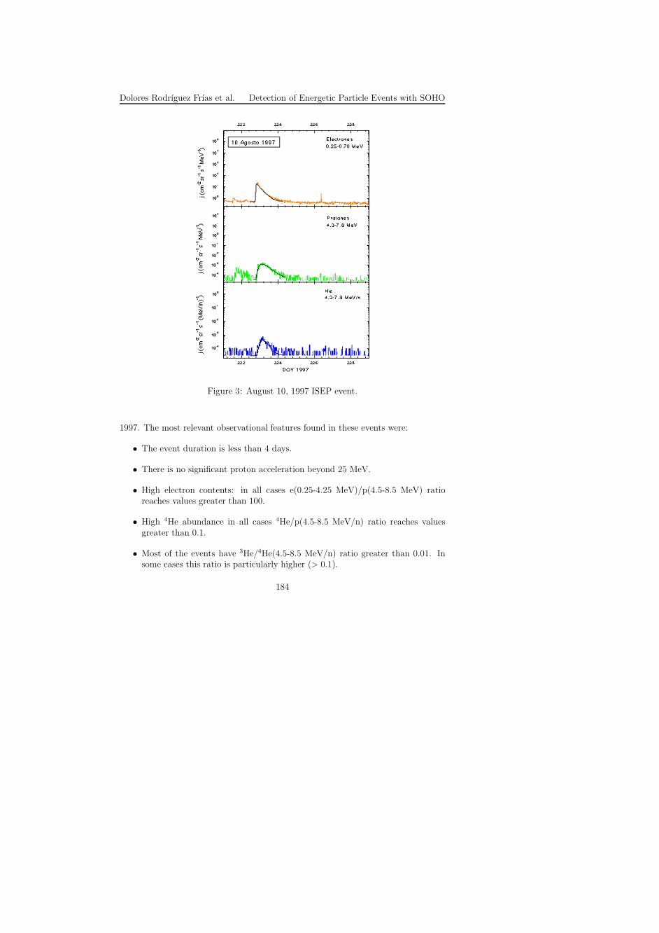
Dolores Rodrıguez Frıas et al. Detection of Energetic Particle Events with SOHO
Figure 3: August 10, 1997 ISEP event.
1997. The most relevant observational features found in these events were:
• The event duration is less than 4 days.
• There is no significant proton acceleration beyond 25 MeV.
• High electron contents: in all cases e(0.25-4.25 MeV)/p(4.5-8.5 MeV) ratioreaches values greater than 100.
• High 4He abundance in all cases 4He/p(4.5-8.5 MeV/n) ratio reaches valuesgreater than 0.1.
• Most of the events have 3He/4He(4.5-8.5 MeV/n) ratio greater than 0.01. Insome cases this ratio is particularly higher (> 0.1).
184

Dolores Rodrıguez Frıas et al. Detection of Energetic Particle Events with SOHO
Figure 4: Temporal profiles of the November 28, 1997 ISEP event.
• In general, they have not associated neither CMEs nor interplanetary shockwaves.
• Proton and 4He spectra are relatively soft (γp < 3.0), except for the November28 1997 event.
Seven events have been classified as gradual: November 28 1996, April 1 1997,April 7 1997, September 24 1997, November 4 1997, November 6 1997 and April 201998. These events present the following signatures:
• The event duration is greater than five days, exceeding 10 days in many cases.
• Protons are accelerated beyond 25 MeV.
• The electron content is, in general, lower than that of impulsive events. Al-though, some events have high electron abundance (April 20, 1998).
185

Dolores Rodrıguez Frıas et al. Detection of Energetic Particle Events with SOHO
• 4He/1H ratio is close to coronal and solar wind abundance (typically between0.02 and 0.05). In some events slight Helium acceleration is observed and theratio becomes lower.
• 3He can not be appreciably above background.
• Most of them have associated CMEs, and interplanetary shock waves (althoughin some cases it has not been possible to find any associated shock). Usuallyshock passage can be seen as transient hardening of spectral index, followed bylong periods of invariant spectrum.
• Proton and 4He spectra are hard (γp < 3.0), except for the November 28 1996event.
November 25 1996, December 24 1997, and September 20 1997 events have mixedfeatures, although the first one seems to be more impulsive and the last two onesmore gradual events. August 13 1996 event shows some peculiarities and it has notbeen classified.
Acknowledgements: This work has been supported by the Ministerio de Ciencia yTecnologıa (MCYT) of Spain, project BXX2000-0784 and the University of Alcala,project UAH2002/081. SOHO is a project of international cooperation between ESAand NASA.
References
[1] Mason et al. 1986, ApJ, 303, 849[2] Reames, D. V. 1993, Adv. Space Res., 13, 331[3] Reames, D. V. et al. 1997, ApJ, 483, 515
186

THE ROLE OF LABORATORY IN
ASTROPHYSICS: LABORATORY
EXPERIMENTS ON ICES AND
ASTROPHYSICAL APPLICATIONS
MIGUEL ANGEL SATORRE, MANUEL DOMINGO, OSCAR GOMIS, RAMONLUNADepartamento de Fısica Aplicada, Escuela Politecnica Superior de Alcoy,Universidad Politecnica de Valencia, E-03801 Alcoy, SPAINMa ANGELES HERNANDEZ-FENOLLOSADepartamento de Fısica Aplicada, Universidad Politecnica de Valencia, E-46022Valencia, SPAIN
Abstract: Laboratory experiments allow the scientific to simulate some of theconditions where the molecules of astrophysical interest are synthesized, and to studylikely mechanisms that could have led to produce them. In a typical astrophysicslaboratory many relevant physical properties (optical constants, density, absorbance,etc) can be studied along with their variations induced by temperature changes andUV or ion irradiation. In this work, we want to offer to the reader a general overviewof the components of a typical astrophysics laboratory. In addition, we will presentsome results obtained after carrying out experiments on ion irradiation of ices. Theseexperiments are carbon implantation in water ice and ion irradiation of methane.Finally, some astrophysical applications are shown to highlight the possibilities ofthis kind of experiments.
1 Introduction
During the last century observational astrophysics has moved from carrying out ob-servations only in the visible region to span a much wider range of the electromagneticspectrum (from gamma rays to radio). As a matter of fact, infrared (IR) observationshave opened the possibility of studying molecules in gas or solid phase [1, 2]. Theimprovement in the resolution of the instruments and space observatories that avoidthe problem of the strong absorption of H2O and CO2 present in our atmosphere,have made possible to identify some molecules in solid state phase such as H2O,CO2, CO and CH4. Physical and spectroscopic properties of such molecules have
187

Miguel Angel Satorre et al. The Role of Laboratory in Astrophysics
been studied both by theoretical and experimental ways [3, 4, 5]. In fact, labora-tory experiments using in-situ IR spectroscopy are a fundamental tool to understandthe space chemistry. In a laboratory, it is possible to simulate adsorption-desorptionprocesses, thermal annealing and UV or ion irradiation [6, 7, 8, 9]. Irradiation playsan important role in the chemical evolution of molecules whose formation reactionsdemand an energetic contribution [10, 11]. Depending on the scenario of interest akind or another of radiation becomes relevant. In the inner part of molecular clouds,protected from the external UV field, ion irradiation is supposed to be the domi-nant mechanism. Our Solar System presents also scenarios where ion irradiation isdominant as the icy Galilean satellites immersed into the intense magnetosphere ofJupiter [12].
In the next sections we will show some results obtained after carrying out ex-periments on ion irradiation of ices. With this objective in mind, some experimentscarried out in the “Laboratorio di Astrofisica Sperimentale di Catania (LASp)” Italy,will be discussed. In section 2 the experimental setup will be described. Ion irradia-tion experiments will be presented in section 3 showing that ion irradiation inducesthe modification of the physical and chemical properties of the ices. Finally, section 4shows some astrophysical applications based in part on the experiments presented insection 3.
2 Experimental setup
The basic components of an astrophysics laboratory are a vacuum and low tempera-ture system, an analysis technique, and for ion irradiation experiments, an ion gun.Figure 1 shows a block diagram of the experimental apparatus present in the LASpwhere all the experiments shown below have been carried out. The main compo-nent is a vacuum chamber (P ∼ 10−7 mbar). Inside the chamber is located a coldfinger whose temperature ranges between 10 and 300 K. The working temperatureis obtained from the balance of two factors. First of all, there is a closed-cycle Hecryostat that is used to cool the substrate down to 10 K. Subsequently, a stationarytemperature is kept by mean a resistor. The vacuum chamber has three windows.Two of them are made of KBr and are faced one to each other. This setup allows usto obtain the transmittance spectrum with a FTIR spectrometer Bruker Equinox-55,with a resolution of 1 cm−1. The third window, perpendicular to the previous ones,let us to irradiate the sample. The surface where the ice is deposited onto, forms 45o
with both the ion and the infrared beams. In this way the sample can be analyzedbefore, during and after irradiation. Gases or mixtures of the molecules under studyare prepared in a pre-chamber in a proportion estimated from their partial pressures.The gases come into the chamber through a needle valve that regulates the flow ofthe gas. The molecules accrete onto the substrate (usually a specular monocrystalline
188

Miguel Angel Satorre et al. The Role of Laboratory in Astrophysics
Figure 1: Block diagram of the experimental apparatus present at the Catania Lab-oratory of Astrophysics.
silicon wafer) put in thermal contact with the cold finger. The thickness of the sampleis monitored by interferometry using an He-Ne laser beam. Since not all the moleculeshave the same sticking coefficient, the final composition of the ice is analyzed by theIR spectrometer. The ice can be irradiated during and/or after deposition, with anion previously accelerated with a 30 kV potential. Deflection plates placed along theions path let us irradiate the sample homogenously. The ion flux is controlled inorder to avoid the macroscopic heating of the sample. The effect of the ion beam onthe ice is monitored continuously with the spectrometer. It is also possible to carryout Temperature Programmed Desorption (TPD) experiments which let us study thesublimation temperature of the deposited and produced molecules. For further detailson the experimental setup see [13, 14].
189

Miguel Angel Satorre et al. The Role of Laboratory in Astrophysics
The experiments here described try to simulate the energetic processes sufferedby the ices in different astrophysical scenarios. Depending on the scenario we areinterested in, composition, thickness and temperature of the ices, and energy andkind of ion can vary vastly. Let’s take as an example the ices present in the denseinterstellar medium (ISM) and on the surface of the Jovian satellite Europa. In thefirst case the thickness of the ice is about tenths of microns while in Europa is morethan nine orders of magnitude greater. As far as the ion flux is concerned, in theJupiter satellite is around six orders of magnitude bigger than in the ISM. On thecontrary, the energy of the most abundant ions in Europa is at least one order ofmagnitude smaller than those in the ISM. The experiments that better reproduce thedense ISM are called thin film experiments because the impinging ions have enoughenergy to pass throughout the sample. On the other hand, experiments that try toreproduce the situation found in a satellite surface or a comet are called thick filmexperiments. In this case, the ion has not enough energy to pass throughout the iceand is implanted into the target [15]. In this situation if the implanted ion is reactive(H+, C+, O+, etc) the new molecules formed could contain the impinging ion [16].
3 Irradiation experiments
In this section some effects of ion irradiation of ices will be shown, in particular thechemical changes induced by ion irradiation.
3.1 Introduction
When a particular ion penetrates inside a material interacts with its atoms loosingenergy as it travels through it. The interaction between the ion and the ice can bedivided in two different types. The first one is electronic (excitations and ionizations)and the second one is nuclear (breaking of bonds and atomic displacements). Thesetwo mechanisms are also called inelastic and elastic respectively. For a detailed de-scription of these processes we refer the reader to Johnson’s book [17]. As said above,as the ion passes through the sample several processes are induced such as local in-creasing of temperature, formation of excited species and ions, etc. Local increasingof temperature is an important effect that must be taking into account when carryingout experiments of astrophysical interest. In space, the number of ions impinging ona surface usually is not enough to produce the macroscopic heating of the same. Onthe contrary, in laboratory one must be sure that the used ion flux is low enough toavoid heating up macroscopically the sample and therefore to produce some unwantedthermal processes.
The effects induced after ion irradiation of ices can be summarized as follows:
190

Miguel Angel Satorre et al. The Role of Laboratory in Astrophysics
• Physical and chemical modifications of the target are produced including theformation of new species.
• In the case of an implantation experiment (thick film), if the used ion is reactive,the possibility exists that the new molecules formed contain the projectile.
• Material is eroded from the target (sputtering).
3.2 Implantation of 13C+ in water ice
Figure 2: H2O ice spectra as deposited and after implantation of 30 keV of 13C+.From left to right, the three spectral regions correspond to H2O, H2O2, and 13CO2
and 13CO bands respectively [10].
Figure 2 shows the results obtained after implantation of 13C+ in water ice at atemperature of 16 K. In the figure are shown three different spectral regions. In thefirst one it is shown the 3.03 µm (3300 cm−1) water ice band and how its area decreasesas ion fluence increases. The decreasing in the water ice band intensity is due to twodifferent effects. The first one is the water ice sputtering. The second one is that
191

Miguel Angel Satorre et al. The Role of Laboratory in Astrophysics
part of the radicals produced by ion irradiation can react to produce new molecules.The second region of the spectrum testifies for the appearance of a new species. Inthis particular case the feature centered at 3.50 µm (2850 cm−1) is attributed to thehydrogen peroxide molecule. In this way we present a case where ion irradiation hasproduced a molecule originally not present in the sample. Finally, the third regionshows that, after the implantation of 30 keV of 13C+, 13CO2 is detected. In thisparticular case, we have found a molecule originally not present that contains theprojectile. As can be seen from the figure, we have also detected for the highest ionfluence 13CO. Taking into account the band intensities and the integrated absorbancesof both 13CO2 and 13CO, we have deduced that 13CO has not been produced directlyby ion implantation of 13C+ but it comes from the destruction of 13CO2. To concludethis section, we would like to point out that ion implantation into an ice not alwaysproduces species containing the impinging ion. As an example, oxygen implantationin frozen methane does not produce neither CO2 nor CO [18].
3.3 Ion Irradiation of CH4 ice
An important kind of compounds suggested to be present in different astrophysicalscenarios are organic molecules. The study of the carbon chemistry has a particularinterest because of its possible implication in the origin of life. In fact, the study ofthe formation of more complex organic compounds such as polymers from elementalmolecules for instance CH4 turns out to be very attractive [19].
Figure 3 shows the results obtained after irradiating with 60 keV of Ar++ ions onpure methane ice at 12 K [11]. The bottom part of the figure shows the spectrumof CH4 deposited at 12 K in two different spectral regions. In the upper part of thefigure the same spectral regions are shown after the CH4 has been irradiated. Inthis experiment the thickness of the CH4 ice is about 4 µm. The amount of energydeposited in average after irradiation (7 eV/16 amu), has been calculated in eV per16 atomic mass units (eV/16amu). This is a convenient way of expressing the dosethat allows to compare results obtained by different authors.
From figure 3 can be observed the appearance of many new IR bands after irradi-ation. These features mainly correspond to new synthesized organic molecules suchas acetylene, ethene, ethane and propane. There are also some weak bands that wehave not been able to assign to any particular species. These latter bands could beattributed to a carbonaceous residue of unknown composition. In the laboratory, ithas been checked that this residue is refractory. In fact, when the temperature of theirradiated sample is increased up to room temperature all the ices sublimate and theonly compound that remains onto the substrate is the residue. This stability at roomtemperature allows to analyze it with other techniques such as UV-Vis spectroscopy,Raman spectroscopy and photoluminescence. We have shown a general result thatcan be summarized as saying that ion irradiation of simple organic molecules produces
192

Miguel Angel Satorre et al. The Role of Laboratory in Astrophysics
Figure 3: Spectra of methane ice as deposited at 12 K (bottom) and after irradiationwith 60 keV Ar++ ions (top) in two different spectral regions.
a progressive carbonization (dehydrogenation) on the original ices.There are some interesting experiments that can be carried out after irradiation of
an ice with ions. By using TPD the sublimation dependence of an ice can be studied.It is known that ices sublimate at different temperatures depending on the matrix themolecule is embedded in. In the case the ice or mixture has been previously irradiatedthe variation of the sublimation temperature can be even greater.
4 Conclusions and astrophysical applications
The effects produced after ion irradiation of ices can be summarized as follows:
• Irradiation destroys sample molecules producing radicals that can then react toform new species.
• In the case a reactive ion is implanted into the ice, the possibility exists that itcould form part of the new synthesized molecules.
193

Miguel Angel Satorre et al. The Role of Laboratory in Astrophysics
• Ion irradiation of organic molecules produces a progressive dehydrogenation ofthe sample. After irradiation a residue is produced. This residue is stable atroom temperature.
• Chemical and physical changes due to ion irradiation increase in some casesthe sublimation temperature of the ices. These variations depend on the icemixture, the used ion and on the irradiation dose.
To conclude we would like to give some examples of astrophysical scenarios whereion irradiation experiments have interest.
The first scenario is the Jupiter satellite Europa. NIMS data from the Galileospacecraft have revealed a feature in the spectrum of Europa’s surface that has beenattributed to the molecule of H2O2. Recent experiments on ion irradiation of waterice have shown that hydrogen peroxide may be produced by radiolysis even if waterice is the only component found on the surface of satellite Europa [12]. The highefficiency for the production of hydrogen peroxide measured for 13C+ and for otherheavy ions, specially for oxygen, opens also the possibility of a patchy distribution onthe surface of the satellite [12]. This result could be useful to support the suggestedpossibility of a radiation-driven ecosystem on Europa based on the availability oforganic molecules and oxidants such as hydrogen peroxide [20].
There are several places in the Solar System such as Pluto and Triton where CH4
ice is present [4] and suffers from ion irradiation. The chemistry induced by lowenergy ions on the uppermost layers of a surface is considered to be quite equivalentto that induced by more energetic cosmic ions at the end of their travel into thicksolid bodies [15]. As an example, it has been evaluated that a fraction of 30 per centof original ice can be altered at a depth of about 10 m within a cometary surface [15].Pluto is in fact exposed to cosmic ions [21] and as a consequence its surface is alteredto a depth of several meters during its total lifetime. On the other hand, low energyions, which have higher fluxes, alter the outer surface layers of the planet in a muchshorter timescale. On Triton the effects could be even more relevant because thesatellite can also be bombarded by ions present in the magnetosphere of Neptune.
Acknowledgements: We thank G. Strazzulla, F. Spinella, G. Baratta, M. E. Palumbo,and G. Leto for their support and help at Catania Astrophysics Laboratory. Withouttheir help this work would have not been possible. This work was partially supportedby the “Ministerio de Ciencia y Tecnologıa, Programa Nacional de Astronomıa yAstrofısica AYA2001–2385” and Universidad Politecnica de Valencia under project“Estancias de PDI de la UPV en Centros de Investigacion de prestigio”.
194

Miguel Angel Satorre et al. The Role of Laboratory in Astrophysics
References
[1] Goicoechea, J. R., Cernicharo, J. 2001, The Promise of the Herschel Space Ob-servatory. Eds. G. L. Pilbratt, J. Cernicharo, A. M. Heras, T. Prusti and R.Harris. ESA-SP, 460, 413
[2] Boogert A. C. A., Ehrenfreund, P. 2004, Insterstellar ices, Astrophysics of dust,ASP Conference Series
[3] Baratta, G. A., Palumbo, M. E. 1998, J. Optical Society of America A, 15, 3076[4] Grundy, W. M. et al. 2002, Icarus, 155, 486[5] Baragiola R.A. 2003, Planet. Space Sci., 51, 953[6] Kimmel, G. A. et al. 2001, J. Chem. Phys., 114, 5295[7] Bahr, D. A. et al. 2003, J. Geophys. Res., 106, 33285[8] Leto, G., Baratta, G. A. 2003, A&A, 397, 7 (2003).[9] Munoz-Caro, G. M. et al. 2002, Nature, 416, 403
[10] Strazzulla, G. et al. 2003, Icarus, 164, 163[11] Baratta, G. A. et al. 2003, NIMB, 209, 283[12] Gomis, O. et al. 2004, Planet. Space Sci., 52, 371[13] Domingo, M. 2003, PhD, Universidad Politecnica de Valencia, Spain[14] Gomis, O. 2003, PhD, Universidad Politecnica de Valencia, Spain[15] Strazzulla, G., Johnson, R.E. 1991, Comets in the Post-Halley Era, R. Newburn
Jr., M. Neugebauer, J. Rahe (Eds.), Kluwer, Dordrecht, 243[16] Strazzulla, G. et al. 1996, NIMB, 116, 289[17] Johnson, R. E. 1990, Energetic Charged Particle Interactions with Atmospheres
and Surfaces. Springer-Verlag, Heidelberg[18] Palumbo, M. E. 1997, Adv. Space Res., 20, 1637[19] Strazzulla, G. et al. 2002, NIMB, 191, 714[20] Chyba, C. F. 2000, Nature, 403, 381[21] Johnson R. E. 1989, Geophys. Res. Letters, 16, 1233
195

Miguel Angel Satorre et al. The Role of Laboratory in Astrophysics
196

ON THE FUTURE OF ULTRAVIOLET (UV)
ASTRONOMY
ANA I. GOMEZ DE CASTROInstituto de Astronomıa y Geodesia (Consejo Superior de Investigaciones Centıficas- Universidad Complutense de Madrid)Facultad de Ciencias Matematicas, Universidad Complutense de Madrid, E-28040Madrid, SPAINWILLEM WAMSTEKERVILSPA-European Space Agency, P.O. Box 50727, E-28080 Madrid, SPAIN
Abstract: The situation of UV astronomy: current facilities, future projects andthe great science to be done is briefly outlined.
1 Introduction
The UV range supplies a richness of experimental data which is unmatched by anyother domain for the study of hot plasma with temperatures in between 104 K and105 K; the high excitation lines and the resonance lines of the most abundant speciesin the Universe are observed in UV. Plasma at these temperatures is observed in allastrophysical environments extending over hot stars, cool stars and planetary atmo-spheres, gaseous nebulae, the warm and hot components of the ISM, circumstellarmaterial, the close environment of black holes of all masses from X-Ray Binaries toNuclei of Galaxies, accretion disks, and the intergalactic medium. In addition, theelectronic transitions of the most abundant molecules, such as H2, are observed inthis range which is also the most sensitive to the presence of large molecules such asthe PAHs. In this brief contribution, the situation of UV astronomy is outlined.
2 The UV facilities
There are three major astronomical facilities working in the UV range: the HubbleSpace Telescope (HST), the Galaxy Evolution Explorer (GALEX) and Far Ultravio-let Spectroscopic Explorer (FUSE). HST and FUSE are observatory missions whileGALEX is mainly devoted to carry out the first all-sky UV survey. Let us summarizethe main characteristics of the UV instrumentation in these missions (see also Table 1for a summary).
197

Ana I. Gomez de Castro and Willem Wamsteker Ultraviolet Astronomy
2.1 HST (1990-...)(URL:www.stsci.edu/hst)
HST is a 2.4 m telescope which was deployed in low-Earth orbit on 1990; it is acooperative project of ESA and NASA. HST is a general purpose telescope witha core program: the accurate determination of the Hubble constant, through theobservations of Cepheid variable stars in the galaxies of the Local Group.
The first generation instruments with UV capabilities were the High Speed Pho-tometer, the Goddard High Resolution Spectrograph and the Faint Object Spectrograph.Currently, the The Wide Field and Planetary Camera 2 (WFPC2), the AdvancedCamera for Surveys (ACS) and the Space Telescope Imaging Spectrograph (STIS) pro-vide access to the UV range both for imaging and spectroscopic work. The WFPC2is a 2-dimensional imaging photometer which covers the spectral range between ap-proximately 115 nm and 1050 nm. It simultaneously images a 150”x150” “L”-shapedregion with a spatial sample of 0.1 arcsec per sample and a smaller 34”x34” squarefield with 0.046 arcsec per pixel. There are 8 UV filters with central wavelength be-tween 130 nm and 333 nm. However, the presence of significant red leaks in the UVfilters, together with the much greater sensitivity and wavelength coverage in the redpart of the spectrum for CCD’s, makes calibration of the UV observations difficult.As a consequence, the prime instruments for UV astronomers are the ACS and theSTIS.
The ACS
The ACS is a third generation HST instrument and includes two channels suitablefor UV imaging:
• a High Resolution Channel (HRC), with a field of view of 26”x29” covering therange from 200 to 1100 nm and a plate-scale of 0.027 arcsec/pixel. There arethree broad band (FWHM ≃ 400 A) UV filters available centered at 220 nm,250 nm and 330 nm.
• a Solar Blind Channel (SBC), with a field of view of 31”x35”, spanning therange from 115 to 170 nm and a plate-scale of 0.032 arcsec/pixel.
• a Solar Blind Channel (SBC), with a field of view of 31”x35”, spanning therange from 115 to 170 nm and a plate-scale of 0.032 arcsec/pixel.
There is also a low resolution (grism) spectroscopic mode available with R∼ 100.
198

Ana I. Gomez de Castro and Willem Wamsteker Ultraviolet Astronomy
The STIS
STIS is the prime ultraviolet instrument on-board the HST. It can be used forimaging, high-spatial resolution long-slit spectroscopy and high spectral resolution(echelle) spectroscopy.
• High resolution, long-slit spectroscopy is available in the 115-310 nm with lowand medium spectral resolutions (∼1000 and ∼15,000, respectively). Slits of52” length and widths between 0.”05 and 2” are available.
• High spectral resolution echelle spectroscopy is available in the 115-315 nmrange with resolutions ∼ 50, 000 and ∼ 114, 000.
• When STIS is used in imaging mode in the UV, the field of view is 25”x25”and the plate scale 0.0246 arcsec per pixel. Few filters are available: threenarrow band filters with FWHM between 7 nm and 8.5 nm, centered in theLα (121.6 nm), the CIII] (190.9 nm) and the MgII (280 nm) lines, plus somecontinuum filters with FWHM = 35 nm, centered at 270 nm and 182 nm, andtwo passband filters.
The wider field of view, the higher sensitivity and the greater selection of filtersmakes of the ACS the preferred instrument for UV imaging. However, STIS provideshigher S/N than the SBC in the far UV and has some narrow band filters which arenot available for the ACS.
2.2 FUSE (1999-...)(URL:fuse.pha.jhu.edu)
FUSE is a NASA-CNES-CSA supported astronomy mission that was launched onJune 24, 1999, to explore the Universe using the technique of high-resolution spec-troscopy in the far-ultraviolet spectral region. The Johns Hopkins University has thelead role in the mission, in collaboration with the University of Colorado at Boulderand the University of California at Berkeley.
FUSE obtains spectra from about 90.5 nm to 118.7 nm. The true resolution hasbeen difficult to assess on-orbit (see URL: fuse.pha.jhu.edu/support/guide/). Thespectral resolving power has been estimated to be R = 20, 000 ± 2000, and is nearlyflat across the entire bandpass.
FUSE was designed with two primary objectives in mind: to study the physicsof the hot component of the Interstellar Medium (ISM) and to estimate how muchdeuterium has been destroyed since the Big Bang.
199

Ana I. Gomez de Castro and Willem Wamsteker Ultraviolet Astronomy
2.3 GALEX (2003-2005)(URL: www.srl.caltech.edu/galextech/)
GALEX is a 50 cm telescope, e.g. a small explorer class mission that is part of NASA’sStructure and Evolution of the Universe theme. GALEX will perform both imagingand low resolution spectroscopy, conducting several types of surveys. GALEX willcomplement the capabilities of space observatories like HST (GALEX has a wide fieldof view), and the UV spectroscopic capabilities of FUSE, both currently in orbit.
GALEX is the first mission to conduct an all-sky survey in the ultraviolet with asignificant sensitivity. Two imaging surveys in a far UV band (135-180 nm) and in anear UV band (180-300 nm) with 3”-5” spatial resolution will be carried out to 20-21mag (AB). In addition, a spectroscopic survey in the 135 nm-300 nm band, withspectral resolution ∼ 100 will be done over 100 square degrees. Detailed informationabout all GALEX surveys may be found in the GALEX web page (see above).
The scientific objective of GALEX is to characterize the UV properties of thegalaxies to study their star formation history over the redshift range 0 < z < 2.
3 The next generation of UV astronomy
There are two main facilities under study and/or development at this moment: theInternational Virtual Observatory (IVO) and the World Space Observatory - Ultra-violet (WSO/UV). In addition to these a limited sky survey specifically oriented tointerstellar absorption (TAUVEX) will be launched in 2005 under a collaborationbetween ISA and ISRO.
3.1 The IVO(URL:www.ivoa.net)
There are many projects on-going world-wide to create the so-called Virtual Observa-tories, which basically are computational tools that allow consulting, retrieving andprocessing the information stored in the Astronomical Archives (data from ground-based or space-based observatories, catalogues, etc...) for a given scientific purpose.The IVO alliance tries to coordinate this joint effort world-wide since it is neces-sary to define common standards for the scientific content of the data (astrometric,photometric, spectrophotometric, polarimetric standards) and for the data format. Inaddition, communication technologies ought to be common to all the archives to guar-antee the required interoperability; a rigourous definition of the data is instrumentalfor the meaningful scientific operation of the IVO.
The largest archive of UV data is the Multimission Archive at the Space Telescope(MAST). It provides access to the HST, FUSE and GALEX archives as well as to the
200

Ana I. Gomez de Castro and Willem Wamsteker Ultraviolet Astronomy
Facility Type of Spectral Field Spectral Spatial(lifetime) Instrument Range of view Resolution Resolution
(nm) (arcsec) R
HST Im-ACS(HRC) 200-1100 26x29 Broad band filters 0.”027 pix−1
(1990-...) (FWHM ∼ 40nm)Im-ACS(SBC) 115-170 31x35 0.”032 pix−1
Im-STIS 115-∼350 25x25 Lyα, CIII], MgII 0.”0246 pix−1
Continuum filtersSp-ACS 115-390 Grism 100Sp-STIS 115-310 Long-Slit ∼15000 0.”03 pix−1
(52”) ∼1000115-315 (echelle) 140000
∼50000
FUSE Sp 90.5-118.7 20000±2000(1999-...)
GALEX Im 135-300 All-sky Two broad bands: 3”-5”(2003-2005) NUV(180-300)
and FUV(135-180)Sp 135-300 (grism) 100
Table 1: The main UV facilities working in 2003. Im: Imaging; Sp: Spectroscopy
first UV missions: Copernicus and the International Ultraviolet Explorer (IUE). Also,the data from many small missions are included (see Table 2). The MAST providessome tools for cross consultation of all the UV archives. Also cross-consultation withthe ROSAT (X-ray) archive and some on-line catalogues is implemented.
IVO will allow the cross-consultation of the UV archives with the rest of thearchives spanning the whole spectral range. It will also provide tools to producedirectly scientific results as the Spectral Energy Distributions (SED), spectral lineidentifications and flux determinations or variability studies.
3.2 The WSO/UV(URL:wso.vilspa.esa.es)
The WSO/UV is a 1.7 m telescope mainly designed to be a spectroscopy missiondevoted to high resolution (echelle) spectroscopy (R=50,000) in the 110-340 nm spec-
201

Ana I. Gomez de Castro and Willem Wamsteker Ultraviolet Astronomy
Mission Type of Number of Spectral MainObservations Observations Range Characteristics
(nm)
IUE Sp >10,4000 120-335 Aprox. 10,000 sourcesCopernicus Sp 90-156 & 551 sources,
165-315 mostly bright starsEUVE Sp 7-76 300 sources,
mostly GalacticHUT Spphot 491 91.2-185 Aprox 300 sources.UIT Im 1579 120-330 259 sourcesWUPPE Sp&Pol 467 140-330 169 sourcesBEFS/ORPHEUS Sp 90-190 75 objectsIMAPS/ORPHEUS Sp 600 95-115 10 hot starsTUES/ORPHEUS Sp 239 90-140 62 targets
Table 2: UV data in the MAST archive (from URL:archive.stsci.edu). Sp: Spec-troscopy; Spphot: Spectrophotometry; Im: Imaging; Pol: Polarimetry
tral range. It will also include optical and UV imaging capabilities (see Table 3);long-slit spectroscopic capabilities are under study. The optical design of WSO/UVis optimized to guarantee a maximum light throughoutput (a high effective area) so,although WSO/UV is slightly smaller than HST, it will be an order of magnitudemore sensitive than HST/STIS (at R=50,000). Another important feature for thescience to be carried out with WSO/UV is the orbit; it will be placed in the La-grangian point L2 allowing spectroscopic monitoring which is heavily demanded bythe astronomical community and difficult to carry out with the HST due to its lowEarth orbit. The mission will have a core program focussed in two key problemsfor modern astrophysics: the formation of stars and planetary systems and the cos-mological and chemical evolution of the intestellar and intergalactic medium up toz ≃ 2.
The World Space Observatory Project represents a new space mission concept,since it has grown out directly of the needs of a world wide distributed Astronomicalcommunity which demands access to the UV range after the HST era. Basic scien-tific requirements are improved sensitivity for high spectroscopy and hours-to-daysmonitoring capabilities. WSO/UV will allow to make full profit of the legacy of theprevious UV missions and, especially of the GALEX, first all-sky UV survey.
As WSO/UV has been driven by the needs of scientists from many different coun-tries, a new implementation model was needed to bring the World Space Observatory
202

Ana I. Gomez de Castro and Willem Wamsteker Ultraviolet Astronomy
Instrument Spectral Field Spectral Spatialand Type Range of view Resolution Resolution
(nm) (arcsec) R
HRI 115-310 60 Narrow Band Filters 0.”03 pix−1
Im Lyα,CIV,CIII,MgII(and few more to detemine)
HSI 115-310 300 Broad Band Filters 0.”15Im for surveys (to determine)
OI 360-800 240 (to determine) 0.”12Im
HIRDES 102.8-310.0 50,000Sp
Table 3: The main characteristics of WSO/UV. Im: Imaging; Sp: Spectroscopy
to reality. The developments needed to make the anticipated launch of WSO/UVpossible in 2008 are led by an open international committee of scientists the WorldSpace Observatory Implementation Committee (WIC).
4 A science case for the future
The richness of the UV range is instrumental for the study of all the astronomicalplasmas from few thousands to several hundreth thousand Kelvin. As it is not realisticto attempt to cover all the possible astrophysics in this brief contribution, we shallfocuss on two key problems: the physics of the formation of stars and planetarysystems, and the cosmological and chemical evolution of the intergalactic medium upto z ≃ 2, as an example.
4.1 The physics of the formation of starsand planetary systems
The formation of stars is an accretion process; the gravitational energy of the infallingmaterial is stored in accretion disks which transforms it into radiation, thermal en-ergy and mass ejection (winds). The Magneto-Rotational Instability (MRI) is thesource of turbulence in the disk leading to accretion and outflow. A new paradigm
203

Ana I. Gomez de Castro and Willem Wamsteker Ultraviolet Astronomy
Figure 1:a) The reference model as described in [9] and adapted from Lovelace et al 1995.Magnetic field lines are represented with the corresponding field orientation.
-500 0 500 1000
0
Vr (km/s)
-500 0 500 1000
Vr (km/s)
b) Contribution to the AB Dor C IV[uv1] profile from a normal flare (left) and atransient feature probably associated with a CIR (right). Both events lasted fewkiloseconds. The left profile was observed in three events more during the shortmonitoring time while the last profile was observed only once.Notice the presence of a narrow absorption and the very broad line wings in theright panel profile (see [3] for more details).
204

Ana I. Gomez de Castro and Willem Wamsteker Ultraviolet Astronomy
is emerging in the physics of star formation which properly addresses the relevanceof the magnetic interaction between the stellar magnetic field and the protoplanetarydisk. The interaction disk-magnetosphere basically transforms angular momentum(differential rotation) into toroidal plasmoids which are ejected from the system. Ba-sically all models can be fitted into the basic configuration sketched in Figure 1a;there is a current sheet that separates two distinct regions: an inner stellar outflowand an external disk outflow. Magnetic flux dissipation is expected to be producedin the current layer leading to plasmoids ejections, as well as to the injection of highenergy particles (cosmic rays) in the environment leading to generation of X-raysand ultraviolet radiation. The phenomenon is non-stationary and controlled by twodifferent temporal scales: the rotation period and the magnetic field diffusion timescale. Stellar rotation is a well know parameter which controls the opening of thefield lines towards high latitudes however, plasmoids ejection is controlled by fielddiffusion which is poorly determined (see e.g. [7]). In addition, there is direct evi-dence of infalling gas; the observed velocities are of some few hundreths km s−1, e.g.compatible with free-fall from some few stellar radii. The existence of funnel flowsconnecting the stellar photosphere with the inner accretion disk has been proposed.The infalling material is expected to release its gravitational energy in the shock atthe stellar surface producing hot spots on it.
This outlined paradigm requires to be worked out extensively since many funda-mental issues are left opened, for instance,
1. The development of the MRI depends on the effective coupling with the disk, e.g.on the relative density of free charges. The inner region of disks is sufficientlyionized by the stellar X-rays field, but the outer regions are more problematic.
2. There is a timing problem. If we trust that T Tauri systems are alike our earlysolar system, the meteoric evidence set-up an upper limit of some few 107 yr forplanetesimal differentiation ([11]). Accretion and outflow are observed in manyT Tauri stars 107 yr old. How does MRI co-exist with planetesimal formation?.
3. Numerical simulations show that the star-disk-outflow system is self-regulatingwhen various initial disk densities, stellar dipolar field strengths and primordialfield associated with the disk are tested ([6]) although strong stellar magneticfields may disrupt the inner parts of the accretion disk temporarily.
4. The coexistence of several funnel flows is required to explain the correlationbetween magnetospheric line emission and the accretion rate, however, it isunclear how such a magnetic configuration may be estable and survive in a veryactive environment.
5. Young stars are very active; rapid variations in the X-ray flux are often detected.However, the source of the X-rays variability is poorly known. In solar and space
205

Ana I. Gomez de Castro and Willem Wamsteker Ultraviolet Astronomy
plasmas, it is recognized that such rapid variations may be produced by, at least,three very different physical processes: flares, e.g. magnetic reconnection eventsassociated with the solar magnetic activity), corotating interaction regions orCIRs (shock fronts formed in the interaction between the slow and the fastcomponent of the solar wind) and coronal mass ejections. In the star formationcontext, we often interpret such rapid variations as associated with magneticreconnection events. However, at least in AB Dor, UV spectroscopy has shownto be able to distinguish between bonna-fidae flares and CIRs (see Figure 1band [3]). The monitoring was done with the Hubble Space Telescope and the oldGoddard High Resolution Spectrograph. AB Dor is a 30 Myr old star, in manysenses fairly similar to some Weak line T-Tauri Stars as HD283572.
The only way to get into the scale of the structures represented in Fig 1a (from afraction of R∗ to some 10 R∗) is by means of high resolution spectroscopy (R ≥ 30, 000)of warm plasma (from 10,000 to 100,00 K); e.g. high sensitivity, high resolutionultraviolet spectroscopy (see e.g. [4]).
In addition, UV monitorings are instrumental for the study of this highly non-stationary environment phenomena, as well, as to map the structure of the funnelflows. They may also allow us to understand better the physics of cool active starsin connection with the PMS evolution. The existence of large scale magnetic struc-tures, sling-shot prominences, has been proposed to explain the detection of materialcorotating at some few stellar radii observed in many, rapidly rotating, cool stars(see [2]). In this sense, spectroscopic UV monitorings open the door to the study ofthe interaction of the stellar wind with protoplanetary disks in the early phases whenplanetesimals are differenciated and planets form through the formation of corotatinginteraction regions. Moreover, UV spectroscopy provides fundamental clues on theradiative field in this epoch and its role in the chemical evolution of disk at the timewhen planets are built. The understanding of PMS stars will allow us to understandbetter substellar objects.
4.2 The cosmological and chemical evolution ofthe intergalactic medium up to z ≃ 2
Most of the volume of the Universe, and 80% of the cosmic time, is at redshifts lessthan z ≤ 2. Studies with 10m class ground-based telescopes have shown that in thefirst 20% of the Universe metal abundances are of order 1/100th Solar, and suggest-a marginally significant- increase of metallicity by a factor of ∼ 2 with time, for theredshift range 3.5 < z < 4 ([8]). There remains however, a factor of at least 50-100between the observed [Fe/H] at z = 2 and the current epoch is of prime importance.The limited information on this, combined with the essentially total absence of reliableinformation on the metallicity evolution between 0 < z < 2, leaves a critical gap in the
206

Ana I. Gomez de Castro and Willem Wamsteker Ultraviolet Astronomy
information needed for the discrimination of the evolutionary models of the Universe(e.g. [1]).
The basic enrichment of the primary material from which the current star forma-tion is drawn is a multifaceted problem in which the IGM plays an essential role. Asthe formation of heavy elements is, in all current cosmological models, driven solelyby processes associated with the life-and-death cycles of stars, and as most star for-mation takes place in galaxies, the cycling of metals through the Universe must takeplace on scales which easily exceed the size of galaxies. The IGM contains the mate-rial from which the current galaxies have been formed; the recycling of this materialafter the galaxy and star formation during the period covered by the redshift rangefrom 0 < z < 2, presents the critical link between our current Universe and the epochof structure formation.
As the validity of the Hubble classification diagram for galaxies breaks down atz = 1 ([10]), it is clear that the answer to the question of the connection between thesefirst epochs of structure formation and the current state of the local Universe can onlybe addressed in the epochs between 0.2 < z < 1.7. Only very limited studies havebeen performed in order to clarify the natiure of the metallicity of the IGM at redshiftsz < 3. [5] (loc.cit.) showed that the ionization distribution in the IGM is an essentialparameter in the abundance determination of this diffuse material. The accessibilityof observing at high resolution (R=50,000) and superior S/N for absorption linesassociated with the Lyα forest,and Lyman Limit systems (15 < Log(N(HI)) < 19),the lines of e.g. OIII-VI, CII-IV, NeIV-VI etc. will permit the exploration of the fullrange of ionized and neutral gas out to z = 2. The resolution is a critical parameter,since it must be sufficient to assure that no component mixing occurs.
The impact of the determination of abundance evolution of the gaseous baryoniccontent of the Universe at z < 2 is especially important at a time that the problem ofStar Formation rate in the same redshift range is being addressed by results expectedto be obtained with the GALEX survey. The simultaneous availability of informationon the methal enrichment processes between 0 < z < 2 together with the knowledge ofthe SFR (from the UV-to-SFR coversion) will allow us to constrain the evolutionarymodels.
Acknowledgements: We are indebted to all our colleagues in the World Space Obser-vatory (WSO) Implementation Committee (WIC) (URL:wso.vilspa.esa.es) and in theNetwork for UltraViolet Astronomy (NUVA) (URL: www.mat.ucm.es/∼aig/NUVA/).We all share a common interest in the future of ultraviolet astronomy. Ana I. Gomezde Castro acknowledges the Ministerio of Ciencia y Tecnologıa of Spain for grants.AYA2000-966 and ESP2001-4637.
207

Ana I. Gomez de Castro and Willem Wamsteker Ultraviolet Astronomy
References
[1] Burles, S., Tytler, D., 1998, ApJ, 507, 732[2] Collier-Cameron, A., 2001, in “Recent Insights into the Physics of the Sun and
Heliosphere: Highlights from SOHO and Other space missions”, IAU Symp. 203,eds P. Brekke, B. Fleck, and J. B. Gurman. ASP, p. 229
[3] Gomez de Castro, A.I., 2002, MNRAS, 332, 409[4] Gomez de Castro, A.I., 2004, Astr. & Sp. Sc., 291, in press.[5] Koehler, S., Reimers, D., Wamsteker, W., 1996, A&A, 312, 33[6] Matt, S., Goodson, A.P., Winglee, R.M., Bohm, K.-H.,2002, ApJ, 574, 232[7] Priest, E., Forbes, T., 2000, “Magnetic reconnection : MHD theory and appli-
cations”, New York : Cambridge University Press.[8] Prochaska, J.X., Wolfe, A.M., 2002, ApJ, 566,68[9] Uzdenski, D., 2004, Astr. & Sp. Sc., 291, in press.
[10] van den Bergh, S., 2002, PASP, 114, 797[11] Wadhwa,M., Russell,S.S., 2000, in “Protostars and Planets IV”, University of
Arizona Press; eds Mannings, V., Boss, A.P., Russell, S. S., p. 995
208

NEW GENERATION NEAR INFRARED
SPECTROGRAPHS IN 3.5 m TO 10 m CLASS
TELESCOPES
ARTURO MANCHADOInstituto de Astrofısica de Canarias, E-38200 La Laguna, SPAIN
Abstract: Here we present a review of the new generation near infrared spec-trographs (1 to 5 microns) available in telescopes from 3.5 m to 10 m in diameter.These instruments have in common the new infrared (IR) detectors with a large 1024x 1024 pixel format, low read-out noise and low dark current both in the 1-2.5 and1-5 micron range.
1 Introduction
The study of the spectra of astronomical objects in the Near Infrared (NIR) hasenormous scientific potential: by using NIR, the composition of the dust can beestablished, molecular hydrogen can be studied, and high redshift (z=1) galaxies,whose main emission lines of Active Galatic Nuclei (AGN) (for example, Halpha) liein the NIR region, can also be observed. However, working in this spectral region (1-5microns) is quite a challenge, posing several problems for the astronomer. The firstproblem is the transmission of the sky: since the earth’s atmosphere is dominated bywater vapour, only certain spectral regions can be observed, namely, the J, H, K, Land M band. An additional problem is that a black body with a temperature of 300K will have a very important contribution to the K, L and M band. To avoid thisemission, the whole instrument must be cooled to a temperature below 100 K, whichresults in a myriad of engineering problems to be solved. A third issue is the factthat very fast reads are necessary in order to avoid sky saturation, especially in theL and M band.
During the last 30 years, NIR spectroscopy has been limited by the availabilityof detectors and cryogenic technology. In the 70s only the Circular Variable Pho-tometers (CVF) were available, with very poor resolution (R=100) and very poorthroughput. In the 80s, linear arrays and small bidimensional arrays became avail-able, with very high dark current and read-out noise, which limited their use to brightsources and small spectral ranges. In the mid 90s, new large format arrays with verylow dark current and read-out noise made NIR spectroscopy more similar to theoptical spectroscopy with CCDs in the 80s. NIR spectrographs are very complex
209

Arturo Manchado New Generation of NIR Spectrographs
cryogenic machines, and as a result the number of these spectrographs is currentlyrather scarce. Key points to consider when designing a NIR spectrograph includetarget acquisition and sky subtraction. Target acquisition is difficult due to the im-possibility of using an optical slit view with CCD, since on the one hand differentialsky refraction causes the optical and IR image to be shifted by several arcseconds(depending on the airmass), and on the other hand some sources are very red andtherefore very weak in the optical image. Another factor to take into account is thestrong sky emission in the NIR: for example, the sky emission in the Ks band is 13magnitude per square arcsecond (3 and -0.5 in the L and M bands). Therefore, mostNIR spectrographs have an imaging mode which makes it possible to use in the NIRthe usual imaging technique of dithering the telescope around the target position inorder to subtract the sky emission. As some of these spectrographs aim at very weaktargets, such as MK=20, target acquisition can be a very time-consuming task. Oncethe target is on the slit, the usual beam-switch technique is used; however, to allow forcorrect sky subtraction, beam-switching has to be done every 15 minutes. Thus thesystem (instrument+telescope+autoguider) has to be very stable in order to ensurethat the target will be on the slit after several beam-switches (for a 3-hour integra-tion on one target, 12 beam-switches will be necessary). The other key point is skysubtraction, as this spectral range is dominated by strong atmospheric OH emissionlines. In order to allow for proper sky subtraction, the design should minimize flex-ures which will shift the spectral lines. As an example, the user requirement of LIRISallows maximum flexure of 4-microns between the focal plane and the detector duringone hour of integration time. All this makes the optical and mechanical design farmore complex than that of an optical spectrograph. Regarding spectral resolution,in order to avoid the atmospheric OH lines, the optimal resolution is between 1000and 3000. Another important point is the dispersion element. Some spectrographsuse reflection gratings which provide high resolution, especially if echelle gratings areused, while for low resolution (R=1000) usually grisms (a combination of a prism anda refraction grating) are used.
Array Pixels Pixel size Read out Dark current Working(e−1) (e−1 s−1) Temperature (K)
Hawaii 1024 x 1024 18 15 0.01 70Hawaii-2 2048 x 2048 18.5 15 0.01 70
ALLADIN 1024 x 1024 27 40 0.01 30
Table 1: Characteristics of near-IR arrays
Two different detectors were manufactured in the late 90s, Hg:Cd:Te with a spec-tral coverage from 0.8 to 2.4 microns (Hawaii 1024 x 1024 and Hawaii-2 2048 x 2048,both manufactured by Rockwell), and InSb with a spectral coverage from 1-5 mi-
210

Arturo Manchado New Generation of NIR Spectrographs
crons (ALLADIN 1024 x 1024, manufactured by Raytheon). These detectors requirevery precise temperature control, as their characteristics (bias, hot pixels, etc) canbe altered if there is a difference of even a small fraction of a degree K. For LIRIS itwas found that the optimal operation temperature was 70 ± 0.005 K. The spectraldimensions of NIR spectrographs have been divided into two ranges: 0.8 -2.5 micronswhen using Hawaii arrays, and 1-5 microns when using ALLADIN arrays. The maincharacteristics of these arrays are listed in Table 1. The spectrograhs in the twospectral ranges will be discussed in more detail below.
2 Spectrographs in the 0.8 to 2.4 microns range
Instrument Telescope Plate scale Resolution Pola- MOS Corono-”/pixel rimetry graphy
IRIS2 [3] AAT 0.45 2400 no yes noISSAC [2] VLT 0.15 500-3000 yes no noLIRIS [4] WHT 0.25 1000-3000 yes yes yes
Omega-Cass [1] Calar Alto 0.04,0.3 420,1050 yes no noNICS [5] TNG 0.25,0.13 50-1250 yes no noSOFI [2] NTT 0.14,0.27,0.29 600-1500 yes no no
Table 2: 1-2.5 microns spectrographs
These spectrographs make use of the Hawaii arrays, both the Hawaii and theHawaii-2 (2048 x 2048). These arrays, which can be seen in Table 1, have very lowreadout noise and very low dark current, thus the observations are usually limitedby background noise for integrations longer than 100 seconds. The low dark currentcombined with the spectral resolution make long integration times possible. Thus,these spectrographs make observations which are very similar to the observations inthe optical wavelength.
All these spectrographs use the Hawaii array and have an imaging mode to allowfor target acquisition. They also have full imaging capability with a wide set ofastronomical filters. All except for ISSAC use grisms as disperser elements. Spectraresolution ranges from 50 for NICS to 3000 for ISSAC and LIRIS. All except forIRIS2 have polarimetry modes, and only IRIS2 (in the Southern Hemisphere) andLIRIS (in the Northern Hemisphere) have Multi-Objects (MOS) mode. LIRIS is theonly spectrograph with coronographic mode, whereas ISSAC is the only spectrographwith two arms, one covering the 1-2.5 micron region and the other covering the 2.5-5micron region. The diameters of the telescopes range from 3.5m (Calar Alto, NTTand TNG) to 8m (VLT).
211

Arturo Manchado New Generation of NIR Spectrographs
Instrument Telescope Plate scale Resolution Pola- Corono-”/pixel rimetry graphy
CISCO/OHS [9] SUBARU 0.105 400 no noCONICA [2] VLT 0.01,0.05 400-1100 yes yesGNIRS [7] Gemini S. 0.15 1000-3000 yes noIRCS [9] SUBARU 0.022,0.058 120-5000 no noISSAC [2] VLT 0.075 500-3000 yes no
NIRCSPEC [6] Keck 0.19 2000-20000 no noNIRI [7] Gemini N. 0.02,0.11 460,1650 no no
PHOENIX [7] Gemini S. 0.23 50000 no noUIST [8] UKIRT 0.06,0.12 475-2000 yes no
Table 3: 1-5 microns spectrographs
3 Spectrographs in the 1 to 5 microns range
All these spectrographs use the ALLADIN detector. CONICA is used in combina-tion with the adaptive optics (AO) system NAOS while NIRI is used with the AOsystem Altair. IRCS can be also used with the SUBARU AO system. Spectral reso-lution varies from 120 for IRCS, to 50000 for PHOENIX. CONICA, GNIRS, ISSAC,and UIST all have polarimetry modes, with CONICA being the only spectrographwith coronography mode. UIST is the only one with an Integral Field Unit (IFU).CISCO/OHS has an OH suppressor that removes the OH airglow lines which domi-nate the broad-band background. This gives a gain in sensitivity in the order of 0.5magnitude in the J and H band. None of the spectrographs have MOS modes.
4 Future
Here we describe several other instruments which are being developed at present andwill be operative in the near future. SINFONI, which will be on the VLT, uses aHawaii-2 and has an IFU with 32 x 32 spatial pixels and 2048 spectral channels (firstlight in 2004). CRIRES, which will be on the VLT, will work in the 1-5 micronrange with a 1024 x 4096 pixels array, giving a resolution of R=50000 (first light in2004). LUCIFER, on the BLT, will use the Hawaii-2 array and have a resolutionof R=10000-36000, as well as MOS mode (first light 2004). OSIRIS, on the Keck,will use a Hawaii-2 array, and have an IFU (64 x 16 spatial elements) and an OHsuppressor with a resolution of R=3800. FLAMINGOS on the 4m Mayal (NOAO),uses a Hawaii-2, and will have R=1800 and a MOS mode. EMIR, which will be onGTC, uses a Hawaii-2 and will have a MOS mode with a FOV of 6 x 6 arcminutesand R=3000 (first light 2008).
212

Arturo Manchado New Generation of NIR Spectrographs
Acknowledgements: This work was supported by the Subdireccion General de Proyec-tos de Investigacion under grant AYA2001-1658.
References
[1] http://www.mpia-hd.mpg.de/Public/CAHA/Instruments/index.html[2] http://www.eso.org/instruments/[3] http://www.aao.gov.au/iris2/iris2 why/[4] http://www.iac.es/proyect/LIRIS[5] http://www.tng.iac.es/instruments/nics/nics.html[6] http://www2.keck.hawaii.edu/inst/[7] http://www.gemini.edu/sciops/instruments/[8] http://www.jach.hawaii.edu/JACpublic/UKIRT/instruments/uist/uist.html[9] http://www.naoj.org/Observing/Instruments/index.html
213

Arturo Manchado New Generation of NIR Spectrographs
214

Author Index
Arcay, B., 153
Beckman, J. E., 43
Carricajo, I., 153Cerrato, Y., 165Cid, C., 165Cornide, M., 119Crespo-Chacon, I., 119
Dafonte, C., 153De Castro, E., 119Del Peral, L., 177Domingo, M., 187
Fernandez-Figueroa, M.J., 119
Galvez, M.C., 119Gomez de Castro, A.I., 197Garcıa-Melendo, E., 63Garcıa–Berro, E., 23Garrido, R., 133Gomis, O., 187Gutierrez, J., 177Gomez Herrero, R., 177
Hernan-Obispo, M., 119Hernandez-Fenollosa, M. A., 187Hidalgo, M. A., 165Hueso, R., 63
Iglesias Groth, S., 105Isern, J., 23
Lopez-Santiago, J., 119Luna, R., 187
MacDonald, J., 133Manchado, A., 209Manteiga, M., 133, 153Montes, D., 119
Moreno, R., 143
Oreiro Rey, R., 133
Perez Hernandez, F., 133Perez-Hoyos, S., 63
Rebolo, R., 1Rodrıguez Lopez, C., 133Rodrıguez Espinosa, J.M., 87Rodrıguez, A., 153Rodrıguez Frıas, D., 177Rojas, J. F., 63
Sanchez-Lavega, A., 63Saiz, E., 165Satorre, M. A., 187
Ulla, A., 133, 143
Vega Beltran, J. C., 43
Wamsteker, W., 197
Zurita, A., 43
215

216

Subject Index
2003aw, 144, 147, 1492RE J0039+103, 1252RE J0725-002, 1262RE J1101+223, 124–1262RE J0743+224, 125, 127
accretion disks, 197, 203, 205accretion process, 203, 205active region, 127, 180–183active stars, 119, 127AD Leo, 128, 129age of the Universe, 23AM CVn, 143–145, 149AM CVn system, 143–149AR Lac, 124Artificial Intelligence, 153, 154Astronomical Archives, 200
BK Psc, 125buckyonions, 105, 107, 111, 113–115BY Dra binary systems, 120, 123
CABS, 123, 125CANARICAM, 98Cassini Orbiter, 68Castor, 130Cataclysmic Variable, 143, 148CE 315, 144–146, 149CELT, 103chromosphere, 119, 127, 128chromospheric lines, 121, 123, 127–129chromospherically active binaries, 123CIRs, 171classical T Tauri stars, 123CMB anisotropies, 4CMB data, 1, 4, 8, 10, 11, 14–16, 19,
20CMB power spectrum, 2, 4, 6, 9, 12, 20CMB temperature, 2, 8
CMEs, 170confined flares, 127convection, 24, 26, 28convection zone, 119cool stars, 119cooling process, 26, 28, 33, 38corona, 119, 127coronal abundances, 178, 180Cosmic Microwave Background (CMB),
1–4, 7, 8, 11, 15, 16, 19, 20cosmological model, 1, 10, 207cosmological parameters, 1, 19, 20CP Eri, 144, 146, 147, 149CR Boo, 143, 144, 146, 147, 149critical density, 11crystallization, 26–30, 32, 33, 38CTTS, 123
dark matter, 1, 10, 11, 15database, 153, 155, 161, 163deep models, 71density fluctuations, 1, 2, 11Dst index, 166dynamo mechanism, 119
EC14026, 135–137EHB, 134, 137, 138ejecta, 171ELMER, 99EMIR, 101equivalent width, 128eruptive flares, 127ES Cet, 144, 148, 149EUV, 125expert systems, 153, 154, 156, 162, 163EZ Peg, 124
flare, 120, 121, 125–129foreground emission, 4, 7
217

fullerenes, 105–110, 112, 113, 115fuzzy logic, 153, 156, 162
galaxy bar, 43, 44, 50, 51, 53, 57–59galaxy bulge, 43, 44, 49, 51, 52, 55, 57galaxy disc, 43–45, 47, 49, 52, 55Galileo Orbiter, 68GEMINI, 90General circulation models, 71geomagnetic storm, 165giant planets, 63Gl 687B, 128GP Com, 143–146, 149Gran Telescopio Canarias, 87GSMT, 103
HD 209458b, 64, 82HD 95559, 124–126Helium Cataclysmic Variable, 143Horizontal Mount, 89hot Jupiters, 64hot subdwarfs, 133, 134, 137, 138HP Lib, 144, 145, 149HR 1099, 128Hubble constant, 10Hyades, 130
IC 2391, 130ices, 189II Peg, 127infrared (IR) detectors, 209Interacting Binary DB White Dwarf star,
143, 144, 146–148interferometer, 1, 3, 4, 7interferometric measurements, 4interplanetary medium, 180interstellar medium, 105, 107–109, 111,
113–115ion irradiation, 190IR spectroscopy, 188
Jupiter, 63
Keck, 90KL Dra, 144, 147, 149
large telescopes, 87late-type stars, 119Libraries of stellar spectra, 121, 131lithium abundance, 122Local Association, 130LQ Hya, 128luminosity classes, 156, 159, 160
M dwarfs, 128magnetic field, 177magnetic pressure, 127magnetic reconnection, 119, 127magnetospere, 177microflares, 121microflaring, 124MK system, 154moving group, 130Mt. Wilson, 87
near infrared (NIR) spectrographs, 209–211
neural networks, 153, 154, 157–163neutrino mass, 15, 16NIR spectroscopy, 209
OSIRIS, 97OWL, 103
Palomar, 88particle events, 177, 178, 182photosphere, 119, 126, 128plages, 121Pleiades, 130pre-main sequence stars, 120, 123primordial anisotropies, 2prominences, 121pulsations, 33, 133, 135–139PW And, 130
radial velocities, 122
218

radiative levitation, 24, 25Roche Lobe, 143ROSAT, 123, 125rotation curve, 43, 44, 47, 48, 50, 52–
56, 58, 61rotational velocities, 122RS CVn binary systems, 120, 123, 127,
128RX J0806.3+1527, 144, 148, 149
Saturn, 63sdB, 134–140sdO, 134, 137–140sdOB, 134, 139semiconvection, 27, 28shallow layer models, 71SOHO, 177–179, 182, 183, 186solar flares, 126, 127space mission, 202space weather, 165spectral classification, 154, 156, 157spectral subtraction technique, 121, 123spectral types, 153, 156, 159, 160, 163spectroscopic observations, 120spectroscopy, 127spiral arm, 44, 56, 58star formation rate, 34–36, 38, 43stellar age, 122stellar atmosphere, 126stellar flares, 120, 126–129stellar kinematic group, 120, 130stellar population, 44, 45, 49stellar rotation, 119structural models, 137, 139, 140SUBARU, 90supercluster, 130surface brightness, 56, 58–60synthetic spectra, 153, 160, 161, 163
T-Tauri, 206Taurus-Auriga, 123Taylor-Proudman theorem, 71
transition region, 119
Ursa Mayor, 130UV astronomy, 197, 200UV Cet type stars, 120, 126, 128UX Ari, 127
V1054 Oph, 128V407 Vul, 144, 147–149V789 Mon, 126V803 Cen, 143, 144, 146, 147, 149velocity gradient, 43, 58–60Virtual Observatories, 200VLT, 90Voyagers, 66
weak-lined T Tauri stars, 120, 123White Dwarf, 23–26, 28–34, 36–39WTTS, 123
X-ray, 125
219

220

Astrophysics Symposium Photos
221