Lecture Notes 4

The Monetary Approachunder Rational Expectations

International Economics: Finance Professor: Alan G. Isaac

4 MAFER and RATEX 14.1 Expectations and Exchange Rates . . . . . . . . . . . . . . . . . . . . . . . . 2

4.1.1 Fundamentals . . . . . . . . . . . . . . . . . . . . . . . . . . . . . . . 54.2 Rational Expectations . . . . . . . . . . . . . . . . . . . . . . . . . . . . . . 7

4.2.1 The Rational Expectations Algebra . . . . . . . . . . . . . . . . . . . 84.2.2 The Role of News . . . . . . . . . . . . . . . . . . . . . . . . . . . . . 114.2.3 Another Representation of the Algebra . . . . . . . . . . . . . . . . . 11

4.3 An Observable Solution . . . . . . . . . . . . . . . . . . . . . . . . . . . . . 124.4 The Data Generating Process . . . . . . . . . . . . . . . . . . . . . . . . . . 14

4.4.1 Anticipating Future Fundamentals . . . . . . . . . . . . . . . . . . . 164.4.2 Finding An Observable Reduced Form: The Algebra . . . . . . . . . 17

4.5 An Empirical Application . . . . . . . . . . . . . . . . . . . . . . . . . . . . 214.6 Concluding Comments . . . . . . . . . . . . . . . . . . . . . . . . . . . . . . 22

Terms and Concepts . . . . . . . . . . . . . . . . . . . . . . . . . . . . . . . 23Problems for Review . . . . . . . . . . . . . . . . . . . . . . . . . . . . . . . 25

.1 The Data Generating Process:Detailed Analysis . . . . . . . . . . . . . . . . . . . . . . . . . . . . . . . . . 28

2 LECTURE NOTES 4. MAFER AND RATEX

We have seen that expectations of future inflation are an important determinant of thecurrent exchange rate. This creates a very serious difficulty for research on exchange ratedetermination, since we know very little about expectations formation. In this course, we willconsider several different ways that economists have struggled to grapple with this difficulty.The first approach we consider is the rational expectations hypothesis: the expectations ofindividuals are assumed to match the predictions of our model. It would more accurate tocall these expectations model consistent, but the convention of calling them ‘rational’ is wellestablished among economists. This handout offers a further exploration of the link betweenexchange rates and expectations, when expectations formation is “rational” in this restrictedsense.

4.1 Expectations and Exchange Rates:

The Monetary Approach

In handout 3 we explored the crucial role of expectations in the determination of exchangerates. In order to characterize the economic outcomes of anticipated monetary policychanges, we had to pin down the process of expectations formation. The approach weadopted was to assume expectations were a good match with actual outcomes. In a nutshell,that is the rational expectations hypothesis. The rational expectations hypothesis is thatthe expectations relevant to economic outcomes are appropriately proxied by the forecastsderived from the economist’s model.

To keep the algebra as simple as possible, we will work with the log-linear version ofthe monetary approach model. Recall that there are two basic components of the monetaryapproach to the determination of flexible exchange rates: purchasing power parity, and theclassical model of price determination.

We begin with the log-linear representation of purchasing power parity.1

st = qt + pt − p∗t (4.1)

As always, PPP says that the spot rate is proportional to the relative price level, where thefactor of proportionality is the exogenous real exchange rate.

Next we consider the log-linear representation of the relative price level, as determinedby the Classical model.2

pt − p∗t = ht − h∗t − [φ(yt − y∗t )− λ(it − i∗t )] (4.2)

As always, the Classical model tells us that the relative price level is determined by relativenominal money supplies and relative real money demands.

Together these two components yield our crude monetary approach model of exchangerate determination.

st = qt + ht − h∗t − φ(yt − y∗t ) + λ(it − i∗t ) (4.3)

1For the moment, we are not imposing a constant real exchange rate, but we do continue to treat it asexogenous.

2Here we work with the simplest version, which equates the foreign and domestic money demand param-eters.

4.1. EXPECTATIONS AND EXCHANGE RATES 3

In handout 3 we looked at some of the empirical applications of this simple model. Onepotential problem for empirical tests of the crude monetary approach model is that it maymistake other influences on the exchange rate for a the response to the interest rate. areaffected by monetary policy.

For example, the empirical version of the model allows for random shocks to moneydemand. Let ut be the money demand shock at time t, so that

st = qt + ht − h∗t − φ(yt − y∗t ) + λ(it − i∗t )− ut

The money demand shocks (ut) affect the current price level and thus the current exchangerate, but they also influence expected future inflation and thus the interest differential. Forexample, suppose ut is completely temporary (no serial correlation). Then a positive shockwill increase money demand and lower the price level today, but next period the shock willbe absent and the price level will rise again. So a positive money demand shock will haveboth a direct and indirect effect on the spot rate: by raising money demand it appreciatesthe exchange rate, but by raising expected future inflation (and the interest differential) itdepreciates the exchange rate. Since the observable interest differential will be positivelycorrelated with the unobserved money demand shocks, the estimate of λ will be biaseddownward.3

There are other difficulties as well. For example, there is the question of which inter-est rate should be used empirically, out of the array of possibilities. In this section wealgebraically derive the predictions of the monetary approach to flexible rates under the ra-tional expectations hypothesis. This allows us to overcome some of the problems that haveconcerned us, although it raises a few new questions as well.

We begin by recalling the covered interest parity condition from handout 2.

it − i∗t = fd t (4.4)

In handout 2 we also decomposed the forward discount into two pieces: the expected rate ofdepreciation and the risk premium.

fd t ≡ ∆set+1 + rpt (4.5)

Recall that ∆set+1 represents the expectation at time t of the percentage rate of depreciation

of the spot rate over the period t to t+ 1.Equations (4.4) and (4.5) imply that the interest differential also bears a simple relation-

ship to expected depreciation and the risk premium.

it − i∗t = fd t

= ∆set+1 + rpt

(4.6)

We use the resulting expression to substitute for the interest differential in our crude mone-tary approach model. Substituting (4.6) into (4.3) yields

st = qt + ht − h∗t − φ(yt − y∗t ) + λ(∆set+1 + rpt)− ut (4.7)

3This was noted by Driskill and Sheffrin (1981) and, in a similar context, Sargent (1977).

4 LECTURE NOTES 4. MAFER AND RATEX

4.1.1 Fundamentals

Let us combine all the exogenous determinant of the exchange rate into a single variable, m.

mtdef= qt + ht − h∗t − φ(yt − y∗t ) + λrpt − ut (4.8)

We will refer to m as the exchange rate fundamentals. This allows us to rewrite (4.7) in aslightly simpler form.

st = mt + λ∆set+1 (4.9)

Equation (4.9) expresses the spot exchange rate in terms of the exchange rate fundamentalsand expected depreciation. We see that an increase in expected depreciation causes thespot rate to depreciate: expectations are a crucial determinant of the spot rate. The spotrate is determined by the exchange rate fundamentals and expectations. Unless λ = 0, thefundamentals alone are not enough to determine the exchange rate.

Note that (4.9) implies that if no depreciation is expected, then exchange rate fundamen-tals directly determine the exchange rate (by determining the relative price level, of course).Changes in the exchange rate are very hard to predict, and when we have no reason to be-lieve that depreciation or appreciation is more likely, our best guess may well be that it willremain unchanged. (That does not mean that we think the exchange rate will not change;it is just the guess that is best on average no matter how it actually does change.) In suchcases we may say, roughly, that the exchange rate is believed to follow a random walk: eachperiod it is just as likely to rise as to fall, and we have no reason to bet on a movement inone direction rather than another.

This situation presents obvious difficulties for empirical work: expectations are not ob-servable. There are many proposals to deal with this, but we will only mention two. First,we might ask market participants what their expectations are. That is, we might rely onsurveys. Although such suggestions seem to have recently gained some ground, traditionallyeconomists have rejected this approach. Instead, there has been a tendency to finesse theobservability problem by modeling expectations formation. At this point, most economiststurn to the rational expectations hypothesis.

While (4.9) is helpful conceptually, it is not a complete solution of our model: expecteddepreciation can be decomposed into the current spot rate and the expected future spot rate.

∆set+1 = se

t+1 − st (4.10)

We can therefore rewrite (4.9) as

st = mt + λ(set+1 − st) (4.11)

Solving for the spot rate yields

st =1

1 + λmt +

λ

1 + λse

t+1 (4.12)

Once again this solution drives home a key message: the current level of the spot ratedepends on its expected future value.

Comment: Mark defines γ = 1/(1 + λ) and ψ = λ/(1 + λ).

4.2. RATIONAL EXPECTATIONS 5

4.2 The Monetary Approach under Rational Expecta-

tions

In handout 3, we derived predictions of the monetary approach by relying on a close rela-tionship between expectations about the money supply and its actual evolution. Much of theempirical work on the monetary approach proceeds in this fashion, and the close relationshipis often referred to as “rational” expectations. This section contains an algebraic presenta-tion of the monetary approach to exchange rate determination under rational expectations.The rational expectations hypothesis (REH) is that the expectations relevant to economicoutcomes are appropriately proxied by the forecasts derived from the economist’s model.Let Et denote a mathematical expectation conditional on all information available at timet (including past values of the fundamentals and the structure of the model). Then for themonetary approach, we will represent the rational expectation hypothesis by

set+1

def= Etst+1 (4.13)

The REH renders the expected future exchange rate one of the variables explained by themodel. This is an apparently simple way of endogenizing the expectatations of the future,but it has very strong implications. We will show that it implies that the entire expectedfuture of the economy is relevant to the current spot rate. Specifically, as noted by Bilson(1978, p.78), it implies that the current spot rate is a weighted sum of all expected futureexchange rate fundamentals:

st =1

1 + λ

∞∑i=0

(λ

1 + λ

)i

Etmt+i (4.14)

Since the weights decline over time, just as in a discounted present value calculation, this isoften referred to as the “present value” solution for the spot exchange rate.

Equation (4.14) is the solution for the spot exchange rate under rational expectations.Since it involves expectations of future fundamentals, it is not yet clear how we can use thissolution in empirical work. Before addressing that question, you may want to work throughthe algebra that gives us (4.14). (Otherwise, skip ahead to section 4.3.)

4.2.1 The Rational Expectations Algebra

This section derives the spot rate solution (4.14).Recall our solution (4.12) for the monetary approach model:

st =1

1 + λmt +

λ

1 + λse

t+1 (4.12)

We will combine this with (4.13), our rational expectations hypothesis.

set+1 ≡ Etst+1 (4.13)

The result is (4.15).

st =1

1 + λmt +

λ

1 + λEtst+1 (4.15)

6 LECTURE NOTES 4. MAFER AND RATEX

We are going to use (4.15) to express the spot rate in terms of fundamentals. Our firstapproach will use “recursive substitution.” We begin the the observation that (4.15) appliesat each point in time. Therefore it implies (4.16).

st+1 =1

1 + λmt+1 +

λ

1 + λEt+1st+2 (4.16)

This is just the same relationship, one period forward in time. Taking expectations (at timet) of both sides of (4.15) yields equation (4.18).

Etst+1 = Et

{1

1 + λmt+1 +

λ

1 + λEt+1st+2

}=

1

1 + λEtmt+1 +

λ

1 + λEtEt+1st+2

(4.17)

st =1

1 + λmt +

λ

1 + λ

1

1 + λEtmt+1 +

(λ

1 + λ

)2

EtEt+1st+2 (4.18)

Of course, now we need to substitute for Et+1st+2, and then Et+2st+3 etc. Then we haveafter n substitutions we have

st =1

1 + λmt +

λ

1 + λEt{

1

1 + λmt+1}

+ · · ·

+

(λ

1 + λ

)n

EtEt+1 · · · Et+n−1{1

1 + λmt+n}

+

(λ

1 + λ

)n+1

EtEt+1 · · · Et+nst+n+1

(4.19)

The Law of Iterated Expectations says that Et{Et+ist+i+1} = Etst+i+1. This just meansthat your current best guess of your future best guess about the future spot rate is just yourcurrent best guess about that future spot rate. In otherwords, your current guess uses allthe information you have available, and therefore differs from your future best guess onlydue to new information you will receive in the future and cannot use now. This allows us tosimplify (4.19).

st =1

1 + λ

n∑i=0

(λ

1 + λ

)i

Etmt+i +

(λ

1 + λ

)n+1

Etst+n+1 (4.20)

Noting that λ/(1 + λ) < 1, we often assume limn→∞[λ/(1 + λ)n+1]Etst+n+1 = 0.4 Then wecan write our solution as

st =1

1 + λ

∞∑i=0

(λ

1 + λ

)i

Etmt+i (4.21)

4The situation is actually a bit more complicated than this suggests: see the discussion of “bubbles” insection ??. For now, we assume the weighted sum of expected future fundamentals will converge.

4.2. RATIONAL EXPECTATIONS 7

Bubbles

Noting that λ/(1 + λ) < 1, we assumed above that limn→∞[λ/(1 + λ)n+1]Etst+n+1 = 0.However, we can imagine exchange rate “bubbles” that would generate a non-zero limit forthis term. In this section we offer a simple illustration of this possibility.

Let sf be the present value solution. That is

sft

def=

1

1 + λ

∞∑i=0

(λ

1 + λ

)i

Etmt+i (4.22)

Next define a bubble bt as the following explosive first-order autoregressive process:

bt =1 + λ

λbt−1 + ηt (4.23)

Here ηt is white noise (i.e., mean zero and constant variance). So

Etbt+1 =1 + λ

λbt (4.24)

We propose that sft + bt, which we will call the bubble solution, is a solution to our

rational expectations model. We check this by seeing if it satisfies (4.15). That is, does ourproposed solution satisfy (4.15)?

sft + bt

?=

1

1 + λmt +

λ

1 + λEt

(sf

t+1 + bt+1

)(4.25)

bt?=

λ

1 + λEtbt+1 (4.26)

bt = bt (4.27)

The last equality follows from (4.24). So we see that the bubble solution is also a solutionto our model.

Comment: In his related discussion, Mark uses s instead of s and s instead of sf .

4.2.2 The Role of News

Consider the implication of (4.21) for the difference between the realized spot rate and theanticipated spot rate. Taking expectations at time t− 1 yields

Et−1st =1

1 + λ

∞∑i=0

(λ

1 + λ

)i

Et−1mt+i (4.28)

Subtracting (4.28) from (4.21) yields (4.29).

st − Et−1st =1

1 + λ

∞∑i=0

(λ

1 + λ

)i

(Etmt+i − Et−1mt+i) (4.29)

That is, the difference between the spot rate differs from its anticipated value to the extentthat expectations about the fundamentals have been revised.

8 LECTURE NOTES 4. MAFER AND RATEX

4.2.3 Another Representation of the Algebra

Use of the “forward shift operator” offers a simplified representation of the algebra. Toreduce notational clutter, let µ = λ/(1 + λ) and rewrite (4.15), our characterization of thespot exchange rate in terms of fundamentals and expectations, as (4.30).

st = Et{(1− µ)mt + µst+1}= (1− µ)mt + µEtst+1

(4.30)

Since the expectation at time t of the current spot rate is just the current spot rate, andsimilarly for the current money supply, we can rewrite this as

Etst = (1− µ)Etmt + µEtst+1 (4.31)

Now consider the forward shift operator, F , defined as xt+n = F nxt, and use it to rewrite(4.31) as

(1− µF ) Etst = (1− µ)Etmt (4.32)

Now if we could just multiply both sides by the inverse of (1 − µF ), we would have asolution for the spot rate.5

Etst = (1− µF )−1 (1− µ)Etmt (4.33)

It turns out that we can do this. Define the inverse to be6

(1− µF )−1 = 1 + µF + µ2F 2 + · · ·

=∞∑i=0

µiF i (4.34)

So we can write our reduced form for the spot exchange rate as

Etst = (1− µ)∞∑i=0

µiEtmt+i (4.35)

Of course Etst = st, so we have found our solution for the spot rate.

5More accurately, we would have

Etst = (1− µF )−1 (1− µ)Etmt + ηµ−t

The term ηµ−t is permitted in the solution, since

(1− µF ) ηµ−t = 0

However we will ignore such “bubbles” in the solution.6Note that (1− µF ) (1 + µF + µ2F 2 + · · · ) = 1.

4.3. AN OBSERVABLE SOLUTION 9

4.3 An Observable Solution

We have seen that the exchange rate solution is a weighted sum of expected future funda-mentals. Let us turn to the question of how to use this solution in empirical work. Howcan we handle the expected future fundamentals in the exchange rate solution? Until wecan relate these expected future values to something we can observe and measure, our spotrate solution under rational expectations cannot be turned into a useful empirical model.For example, we cannot offer any simple relationship between the spot rate and the moneysupply (as we attempted to do in handout 3) until we know how the expected future behaviorof the money supply is related to its current and past behavior. Many economists approachthis problem by characterizing the way the fundamentals evolve over time. Such a charac-terization is called a data generating process (DGP) for the fundamentals. This informationcan then be used in forming expectations about the future.

A common assumption in early empirical tests of the monetary approach is that theexchange rate fundamentals follow a random walk:

mt = mt−1 + ut (4.36)

Here ut is the unanticipated change in the fundamentals, which averages zero (and is notserially correlated). This just means that the fundamentals are just as likely to rise as to falleach period. In this case our “best guess” of the future fundamentals is their current value.That is

Etmt+i = mt (4.37)

If the fundamentals are just as likely to rise as to fall, so is the spot exchange rate. Thatis, our best guess of the future spot rate is the current spot rate. Recalling (4.9), we canconclude that

st = mt (4.38)

(This can also be seen algebraically by substituting (4.37) into (4.14).) Recalling the defini-tion of the exchange rate fundamentals, we can then gather data and test (4.38) empirically.

st = q + h− h∗ − φ(y − y∗) + λrp (4.39)

Note how similar this is to the crude monetary approach: only the interest rate effect hasdisappeared.

Obviously the fundamentals cannot always be characterized as following a random walk.For example, if one country consistently has high inflation and another country consistentlyhas low inflation, the random walk characterization of the exchange rate fundamentals forthese two countries will be a poor one. As a result, for many exchange rates we need tocharacterize the exchange rate fundamentals by a more complicated data generating process.For example, we may assume that the fundamentals follow a simple autoregressive process.7

7A more typical way of closing a rational expectations model is much more general: assume that the nexogenous variables follow a kth-order vector autoregressive process (VAR) after differencing. This is a bitmore complicated, so details will be relegated to appendix .1. Briefly, let Xt be the n-vector of exogenousvariables at time t. For example, we might treat relative money supplies and relative incomes as the onlycomponents of our fundamentals. Let X>t = (h − h∗, y − y∗), so we can rewrite our fundamentals as

10 LECTURE NOTES 4. MAFER AND RATEX

Even this considerably complicates the problem of representing and summing up the expectedfuture fundamentals. One useful alternative method for dealing with more general DGPs isthe method of undetermined coefficients, which is briefly treated below.

4.4 The Data Generating Process

Before starting on the algebra, let us get our bearings. Remember, we have a model of thespot exchange rate under rational expectations

s =1

1 + λ(m+ λEts) (4.12)

that provides the basic structure of spot rate determination. We found that we could solvethis model for the spot rate as

st =1

1 + λ

∞∑i=0

(λ

1 + λ

)i

Etmt+i (4.40)

where m represents the exchange rate fundamentals (e.g., relative money supplies and thedeterminants of relative real money demand). Now the problem with this kind of formulationis that it still involves unobserved expectations. While it is informative at the theoreticallevel, it is not very useful empirically. We would like to have an observable solution for theexchange rate, a solution in terms of variables we can observe and measure. To move froma solution like (4.40) to an observable solution, we represent the fundamentals by a datagenerating process (DGP).

For example, we initially treated m as following a random walk, which yielded a simpleobservable solution for the exchange rate. But while this may be a good approximation forsome pairs of countries, for others it will be terrible. (For example, one country might havepersistent high inflation when the other does not.) So consider a more general DGP: thefollowing simple “autoregressive” representation of the fundamentals.

mt = µ0 + µ1mt−1 + ut (4.41)

We will show that given the DGP (4.41), the exchange rate solution is

st =λµ0

1 + λ− λµ1

+1

1 + λ− λµ1

mt (4.42)

mt = a>Xt where a> = (1,−φ). The VAR process simply relates Xt to its past values.

∆Xt =k∑

j=1

Bj∆Xt−j + vt (61)

The B′js are the matrices of coefficients on the lagged exogenous variables and vt is a vector of errors. If wecreate a vector Zt containing the current and lagged exogenous variables, then as shown in appendix .1, oursolution for the exchange rate is a linear function of the current and lagged exogenous variables.

st = a>Xt + a>GC∆Zt (70)

where GC is a matrix defined in appendix .1. This can be estimated simultaneously with (61).

4.4. THE DATA GENERATING PROCESS 11

4.4.1 Anticipating Future Fundamentals

Now if we know the DGP (4.41) governs the evolution of the fundamentals over time, thenin the future we will have

mt+1 = µ0 + µ1mt + ut+1

mt+2 = µ0 + µ1mt+1 + ut+2

mt+3 = µ0 + µ1mt+2 + ut+3

etc.

Forming our expectations in light of this knowledge tells us

Etmt+1 = µ0 + µ1Etmt + Etut+1

= µ0 + µ1mt

Etmt+2 = µ0 + µ1Etmt+1 + Etut+2

= µ0 + µ1(µ0 + µ1mt)

= µ0 + µ1µ0 + µ21mt

Etmt+3 = µ0 + µ1Etmt+2 + Etut+3

= µ0 + µ1(µ0 + µ1µ0 + µ21mt)

= µ0 + µ1µ0 + µ21µ0 + µ3

1mt

...

We quickly see a pattern emerging, which can be summarized by (4.43).

Etmt+i = µ0

i−1∑j=0

µj1 + µi

1mt i ≥ 1 (4.43)

This gives us an important insight. All of our expectations of future fundamentals canbe stated in terms of the current fundamentals.

4.4.2 Finding An Observable Reduced Form: The Algebra

In principle we could substitute our solutions (4.43) for expected future fundamentals intoequation (4.40) and actually perform the summation. This can be very messy, however, sooften it is convenient to rely instead on the method of undetermined coefficients. We will doit both ways.

12 LECTURE NOTES 4. MAFER AND RATEX

Direct Summation

st = (1− µ)∞∑i=0

µiEtmt+i

= (1− µ)∞∑i=1

µiEtmt+i + (1− µ)mt

= (1− µ)∞∑i=1

µi

(µ0

i−1∑j=0

µj1 + µi

1mt

)+ (1− µ)mt

= (1− µ)µ0

∞∑i=1

µi

i−1∑j=0

µj1 + (1− µ)

∞∑i=0

µiµi1mt

(4.44)

So we havest = φ0 + φ1mt (4.45)

where φ0 and φ1 are the constant coefficients that are the infinite sums of structural formparameters in (4.44). It turns out that we can give much simpler representations of thesecoefficients.

Noting that∞∑i=0

µiµi1 =

1

1− µµ1

(4.46)

we have

φ1 =1− µ

1− µµ1

(4.47)

Finding φ0 is a little more work. Let us begin with the inner summation.

i−1∑j=0

µj1 =

1

1− µ1

(1− µi1) (4.48)

Then we can write

φ0 =1− µ1− µ1

µ0

∞∑i=1

µi(1− µi1) (4.49)

Now note that∞∑i=1

µi(1− µi1) =

∞∑i=1

µi −∞∑i=1

µiµi1

=µ

1− µ− µµ1

1− µµ1

=µ(1− µ1)

(1− µ)(1− µµ1)

(4.50)

So we get

φ0 =1− µ1− µ1

µ0µ(1− µ1)

(1− µ)(1− µµ1)

=µµ0

1− µµ1

(4.51)

4.4. THE DATA GENERATING PROCESS 13

Finally, since we have solved for φ0 and φ1, we can write

st =µµ0

1− µµ1

+1− µ

1− µµ1

mt (4.52)

The Method of Undetermined Coefficients

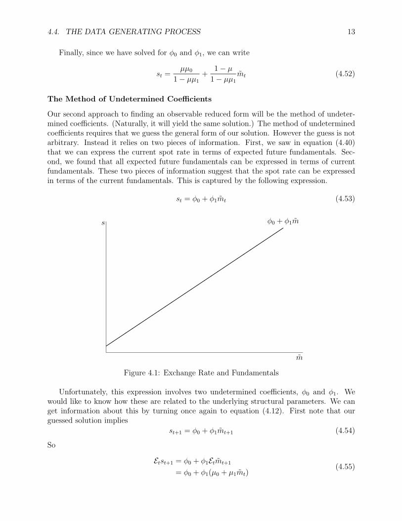
Our second approach to finding an observable reduced form will be the method of undeter-mined coefficients. (Naturally, it will yield the same solution.) The method of undeterminedcoefficients requires that we guess the general form of our solution. However the guess is notarbitrary. Instead it relies on two pieces of information. First, we saw in equation (4.40)that we can express the current spot rate in terms of expected future fundamentals. Sec-ond, we found that all expected future fundamentals can be expressed in terms of currentfundamentals. These two pieces of information suggest that the spot rate can be expressedin terms of the current fundamentals. This is captured by the following expression.

st = φ0 + φ1mt (4.53)

��

��

��

��

��

��

��

��

��

��

��

��

��

�

φ0 + φ1m

m

s

Figure 4.1: Exchange Rate and Fundamentals

Unfortunately, this expression involves two undetermined coefficients, φ0 and φ1. Wewould like to know how these are related to the underlying structural parameters. We canget information about this by turning once again to equation (4.12). First note that ourguessed solution implies

st+1 = φ0 + φ1mt+1 (4.54)

So

Etst+1 = φ0 + φ1Etmt+1

= φ0 + φ1(µ0 + µ1mt)(4.55)

14 LECTURE NOTES 4. MAFER AND RATEX

So we can substitute our expressions for s and se in the undetermined coefficients intoequation (4.12) to get

st =1

1 + λmt +

λ

1 + λEtst+1 (4.56)

φ0 + φ1mt ≡1

1 + λmt +

λ

1 + λ[φ0 + φ1(µ0 + µ1mt)]

=λ

1 + λ(φ0 + φ1µ0) +

1 + λφ1µ1

1 + λmt

(4.57)

Now here is the tricky part. Equation (4.57) must hold for any level of the fundamentalsmt. That is what allows us to determine the φs: the slope and intercept must be the samefor the function of mt that we find on each side of the equality (4.57).

φ0 ≡λ

1 + λ(φ0 + φ1µ0)

φ1 ≡1 + λφ1µ1

1 + λ

(4.58)

These are two equations in the two unknowns φ0 and φ1. The second equation can be solvedfor

φ1 =1

1 + λ− λµ1

(4.59)

so the first gives us

φ0 = λµ0φ1

=λµ0

1 + λ− λµ1

So we can now replace the undetermined coefficients in our guess (4.53) to get

st =λµ0

1 + λ− λµ1

+1

1 + λ− λµ1

mt (4.60)

In empirical work, we can then estimate (4.60) and (4.41) simultaneously.Equation (4.60) has an important message for exchange rate research. There is no simple

relationship between exchange rates and money supplies. Note that the relationship betweenthe spot rate and the money supply depends on all the parameters of the data generatingprocess. For example, if µ1 < 1 so that money supply increases tend to be reversed overtime, then the exchange rate will rise less than in proportion to a money supply increase.

In summary, the method of undetermined coefficients proceeds as follows:

1. Begin with a model and a data generating process (DGP) for the exogenous variables.

2. Based on the DGP, make an educated guess about the functional form of the solution,which will generally involve the exogenous variables, shocks to the system, and possiblylagged endogenous variables. That is, guess an “observable reduced form” for thesystem, where your guess involves “undetermined coefficients” that you want to expressin terms of structural coefficients.

4.5. AN EMPIRICAL APPLICATION 15

3. Find the expectations implied by your proposed solution form.

4. Plug these expectations into the model.

5. Use the implied identities in the coefficients to solve for the undetermined coefficientsin terms of the structural coefficients (here, the µs and λ).

4.5 An Empirical Application

The monetary approach to flexible exchange rates has been tested under the assumptionof rational expectations. After some early results lent some support to the model, a greatdeal of testing took place. Three salient supportive studies are Hoffman and Schlagenhauf(1983), MacDonald (1983), and Woo (1985). Hoffman and Schlagenhauf model fundamentalsindividually as ARIMA(1,1,0) and get pretty good results (1974.1-1979.12) for the dollar vs.the franc, pound, and mark. Woo follows Bilson (1978) in incorporating lagged real balancesin the money demand equation.

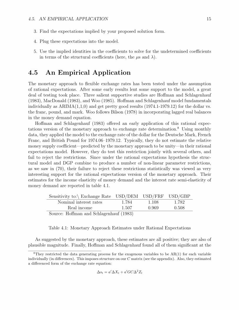
Hoffman and Schlagenhauf (1983) offered an early application of this rational expec-tations version of the monetary approach to exchange rate determination.8 Using monthlydata, they applied the model to the exchange rate of the dollar for the Deutsche Mark, FrenchFranc, and British Pound for 1974.06–1979.12. Typically, they do not estimate the relativemoney supply coefficient—predicted by the monetary approach to be unity—in their rationalexpectations model. However, they do test this restriction jointly with several others, andfail to reject the restrictions. Since under the rational expectations hypothesis the struc-tural model and DGP combine to produce a number of non-linear parameter restrictions,as we saw in (70), their failure to reject these restrictions statistically was viewed as veryinteresting support for the rational expectations version of the monetary approach. Theirestimates for the income elasticity of money demand and the interest rate semi-elasticity ofmoney demand are reported in table 4.1.

Sensitivity to:\ Exchange Rate USD/DEM USD/FRF USD/GBPNominal interest rates 1.784 1.108 1.782

Real income 1.507 0.969 0.508Source: Hoffman and Schlagenhauf (1983)

Table 4.1: Monetary Approach Estimates under Rational Expectations

As suggested by the monetary approach, these estimates are all positive; they are also ofplausible magnitude. Finally, Hoffman and Schlagenhauf found all of them significant at the

8They restricted the data generating process for the exogenous variables to be AR(1) for each variableindividually (in differences). This imposes structure on our C matrix (see the appendix). Also, they estimateda differenced form of the exchange rate equation:

∆st = a′∆Xt + a′GC∆2Zt

16 LECTURE NOTES 4. MAFER AND RATEX

5% level. All in all, this early study appears to provide impressive support for the rationalexpectations version of the monetary approach to flexible exchange rates.

4.6 Concluding Comments

A key lesson of this chapter is that there is no simple relationship between changes in themoney supply and changes in the exchange rate. The effect of a change in the current moneysupply on the current exchange rate depends crucially on its effect on the expected futuremoney supply. So beliefs about the monetary policy “reaction function” will be an importantdeterminant of the contemporary link between exchange rates and money supplies. We willpursue this insight further in handout 11.

In the Classical model, nominal interest rates are determined by expected inflation. Ifindividuals accurately link expected inflation to their anticipations of monetary policy, wecan make more detailed predictions about the behavior of prices over time. This observationcarries over immediately to the monetary approach to exchange rate determination, since inthe monetary appproach PPP ensures that any predictions we make about the behavior ofprices are also predictions about the behavior of the exchange rate.

Terms and Concepts

autoregressive process, 9

data generating process, 8

expectationsmodel consistent, 2rational, 2, 4

fundamentals, 3

monetary approachto flexible rates

with rational expectations, 4under rational expectations

tests of, 14monetary policy

reaction function, 15

random walk, 4, 8rational expectations, see expectations, ratio-

nalrational expectations hypothesis, 4

17

18 TERMS AND CONCEPTS

Problems for Review

1. Suppose mt = µ0 + µ1mt−1 + ut where ut is an unexpected innovation in the datagenerating process. Then Etmt+4 equals

(a) µ0 + µ1Etmt+3

(b) µ0(1 + µ1) + µ21Etmt+2

(c) µ0(1 + µ1 + µ21) + µ3

1Etmt+1

(d) µ0(1 + µ1 + µ21 + µ3

1) + µ41mt

(e) All of the above.

2. Consider the monetary approach to flexible exchange rates under the assumption of“rational” expectations. The current spot exchange rate

(a) depends on all future fundamentals.

(b) depends on all expected future fundamentals.

(c) equals the current value of the fundamentals.

(d) b. and c.

(e) all of the above

3. Use the method of undetermined coefficients to solve for an observable reduced formof the monetary approach to flexible exchange rates under rational expectations. Usethe following DGP: m(t) = 0.8m(t− 1) +u(t) where u(t) is white noise (i.e., is zero onaverage). Show all the steps in your solution procedure.

4. Use the method of undetermined coefficients to solve for an observable reduced formof the monetary approach to flexible exchange rates under rational expectations. Usethe following DGP: mt = 0.8mt−1 + ut where ut = ρut−1 + vt and vt is white noise.How does allowing ut to follow an autoregressive process change the solution?

Bibliography

Bilson, John F. O. (1978). “Rational Expectations and the Exchange Rate.” In Jacob A.Frenkel and Harry G. Johnson, eds., The Economics of Exchange Rates: Selected Studies,Chapter 5, pp. 75–96. Reading, MA: Addison-Wesley.

Driskill, Robert A., Nelson C. Mark, and Steven M. Sheffrin (1992, February). “Some Evi-dence in Favor of a Monetary Rational Expectations Exchange Rate Model with ImperfectCapital Substitutability.” International Economic Review 33(1), 223–37.

Driskill, Robert A. and Steven S. Sheffrin (1981, December). “On the Mark: Comment.”American Economic Review 71(5), 1068–74.

Hoffman, Dennis L. and Don E. Schlagenhauf (1983, March). “Rational Expectations andMonetary Models of Exchange Rate Determination: An Empirical Examination.” Journalof Monetary Economics 11, 247–260. check.

MacDonald, Ronald (1983). “Some Tests of the Rational Expectations Hypothesis in theForeign Exchange Market.” Scottish Journal of Political Economy 30(3), 235–50.

Sargent, Thomas J. (1977, February). “The Demand for Money During Hyperinflationsunder Rational Expectations.” International Economic Review 48, 49–73.

Woo, W.T. (1985). “The Monetary Approach to Exchange Rate Determination under Ratio-nal Expectations: The Dollar-Deutschmark Rate.” Journal of International Economics 18,1–16.

.1 The Data Generating Process:

Detailed Analysis

A typical way of closing a rational expectations model is by assuming that the n exogenous

variables follow a kth-order vector autoregressive process (VAR) after differencing. Thefollowing treatment provides some general tools for implementing this closure.9 Let Xt bethe n-vector of exogenous variables at time t.

∆Xt =k∑

j=1

Bj∆Xt−j + vt (61)

9Much of the development below follows Driskill et al. (1992) fairly closely.

19

20 BIBLIOGRAPHY

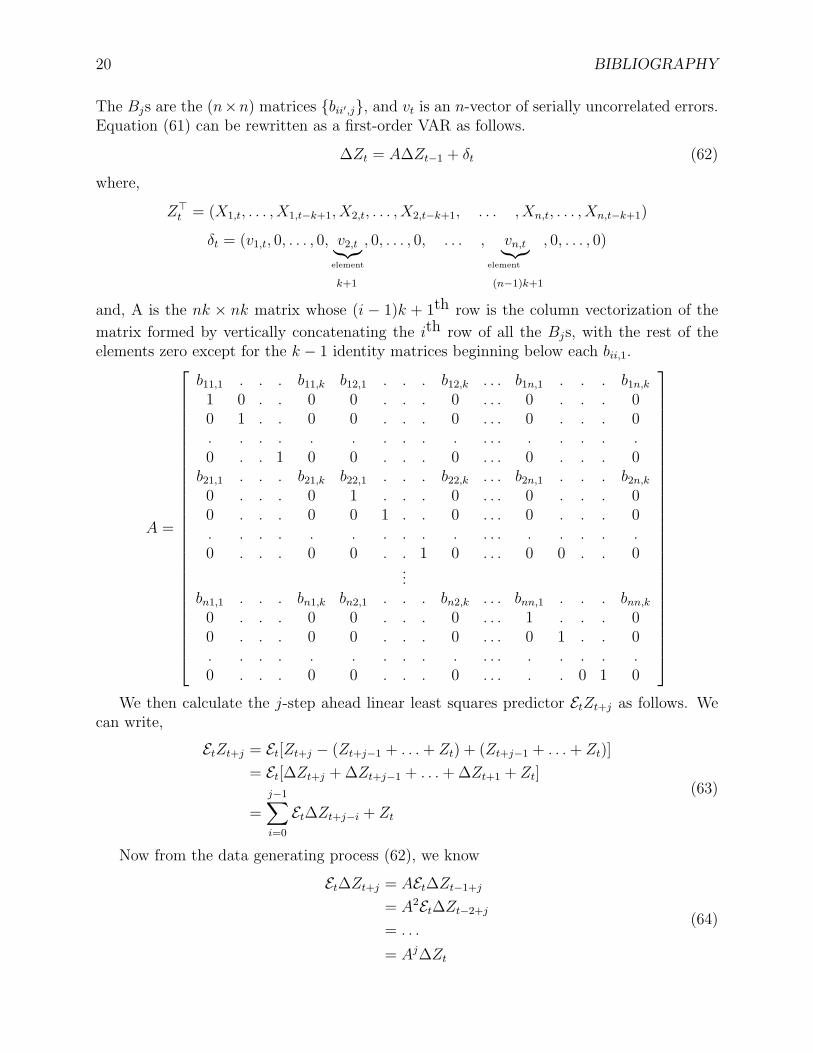
The Bjs are the (n×n) matrices {bii′,j}, and vt is an n-vector of serially uncorrelated errors.Equation (61) can be rewritten as a first-order VAR as follows.

∆Zt = A∆Zt−1 + δt (62)

where,

Z>t = (X1,t, . . . , X1,t−k+1, X2,t, . . . , X2,t−k+1, . . . , Xn,t, . . . , Xn,t−k+1)

δt = (v1,t, 0, . . . , 0, v2,t︸︷︷︸element

k+1

, 0, . . . , 0, . . . , vn,t︸︷︷︸element

(n−1)k+1

, 0, . . . , 0)

and, A is the nk × nk matrix whose (i − 1)k + 1th row is the column vectorization of the

matrix formed by vertically concatenating the ith row of all the Bjs, with the rest of theelements zero except for the k − 1 identity matrices beginning below each bii,1.

A =

b11,1 . . . b11,k b12,1 . . . b12,k . . . b1n,1 . . . b1n,k

1 0 . . 0 0 . . . 0 . . . 0 . . . 00 1 . . 0 0 . . . 0 . . . 0 . . . 0. . . . . . . . . . . . . . . . . .0 . . 1 0 0 . . . 0 . . . 0 . . . 0b21,1 . . . b21,k b22,1 . . . b22,k . . . b2n,1 . . . b2n,k

0 . . . 0 1 . . . 0 . . . 0 . . . 00 . . . 0 0 1 . . 0 . . . 0 . . . 0. . . . . . . . . . . . . . . . . .0 . . . 0 0 . . 1 0 . . . 0 0 . . 0

...bn1,1 . . . bn1,k bn2,1 . . . bn2,k . . . bnn,1 . . . bnn,k

0 . . . 0 0 . . . 0 . . . 1 . . . 00 . . . 0 0 . . . 0 . . . 0 1 . . 0. . . . . . . . . . . . . . . . . .0 . . . 0 0 . . . 0 . . . . . 0 1 0

We then calculate the j-step ahead linear least squares predictor EtZt+j as follows. We

can write,

EtZt+j = Et[Zt+j − (Zt+j−1 + . . .+ Zt) + (Zt+j−1 + . . .+ Zt)]

= Et[∆Zt+j + ∆Zt+j−1 + . . .+ ∆Zt+1 + Zt]

=

j−1∑i=0

Et∆Zt+j−i + Zt

(63)

Now from the data generating process (62), we know

Et∆Zt+j = AEt∆Zt−1+j

= A2Et∆Zt−2+j

= . . .

= Aj∆Zt

(64)

.1. THE DATA GENERATING PROCESS: DETAILED ANALYSIS 21

Combining (63) with equation (64) we get;

EtZt+j = Zt +

j−1∑i=0

Aj−i∆Zt

= Zt +

j∑i=1

Ai∆Zt

Now 10

j∑i=1

Ai = A(I − Aj)(I − A)−1

∴ EtZt+j = Zt + A(I − Aj)(I − A)−1∆Zt (65)

Equation (65) is the j-step ahead linear least squares predictor of Zt.Let G be a (n×nk) matrix of zeros, except for the elements g11, g2,k+1, g3,2k+1, etc. which

are equal to one, then Xt = GZt. Hence, using equation (65) we get the j-step ahead linearleast squares predictor of Xt as follows.

Et(Xt+j) = GZt +GA(Ink − Aj)(Ink − A)−1∆Zt (66)

One more preliminary. It will be useful to note that

A∞∑

j=0

µj(I − Aj)(I − A)−1 = A

(∞∑

j=0

µjI −∞∑

j=0

µjAj

)(I − A)−1

=

[1

1− µI − (I − µA)−1

]A(I − A)−1

=1

1− µ(I − µA)−1[(I − µA)− (1− µ)I]A(I − A)−1

=1

1− µ(I − µA)−1[µ(I − A)]A(I − A)−1

=µ

1− µA(I − µA)−1

(67)

LettingC = µA(I − µA)−1 (68)

we can express this result as

A∞∑

j=0

µj(I − Aj)(I − A)−1 =1

1− µC (69)

10This is the analogue to the scalar result. Recall

n∑i=0

ai =1− an+1

1− a

The sum from 1 to j is a times the sum from 0 to j − 1.

22 BIBLIOGRAPHY

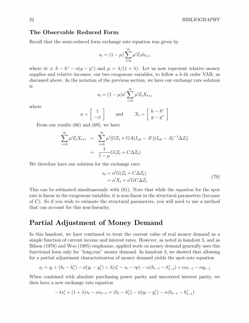
The Observable Reduced Form

Recall that the semi-reduced form exchange rate equation was given by

st = (1− µ)∞∑i=0

µiEtmt+i

where m ≡ h − h∗ − φ(y − y∗) and µ = λ/(1 + λ). Let us now represent relative moneysupplies and relative incomes, our two exogenous variables, to follow a k-th order VAR, asdiscussed above. In the notation of the previous section, we have our exchange rate solutionis

st = (1− µ)a′∞∑i=0

µiEtXt+i

where

a =

[1−φ

]and Xt =

[h− h∗y − y∗

]From our results (66) and (69), we have

∞∑i=0

µiEtXt+i =∞∑i=0

µi[GZt +GA(Ink − Ai)(Ink − A)−1∆Zt]

=1

1− µG(Zt + C∆Zt)

We therefore have our solution for the exchange rate:

st = a′G(Zt + C∆Zt)

= a′Xt + a′GC∆Zt

(70)

This can be estimated simultaneously with (61). Note that while the equation for the spotrate is linear in the exogenous variables, it is non-linear in the structural parameters (becauseof C). So if you wish to estimate the structural parameters, you will need to use a methodthat can account for this non-linearity.

Partial Adjustment of Money Demand

In this handout, we have continued to treat the current value of real money demand as asimple function of current income and interest rates. However, as noted in handout 3, and asBilson (1978) and Woo (1985) emphasize, applied work on money demand generally uses thisfunctional form only for “long-run” money demand. In handout 3, we showed that allowingfor a partial adjustment characterization of money demand yields the spot-rate equation

st = qt + (ht − h∗t )− φ(yt − y∗t ) + λ(set − st − rp)− α(ht−1 − h∗t−1) + αst−1 − αqt−1

When combined with absolute purchasing power parity and uncovered interest parity, wethen have a new exchange rate equation

−λset + (1 + λ)st − αst−1 = (ht − h∗t )− φ(yt − y∗t )− α(ht−1 − h∗t−1)

.1. THE DATA GENERATING PROCESS: DETAILED ANALYSIS 23

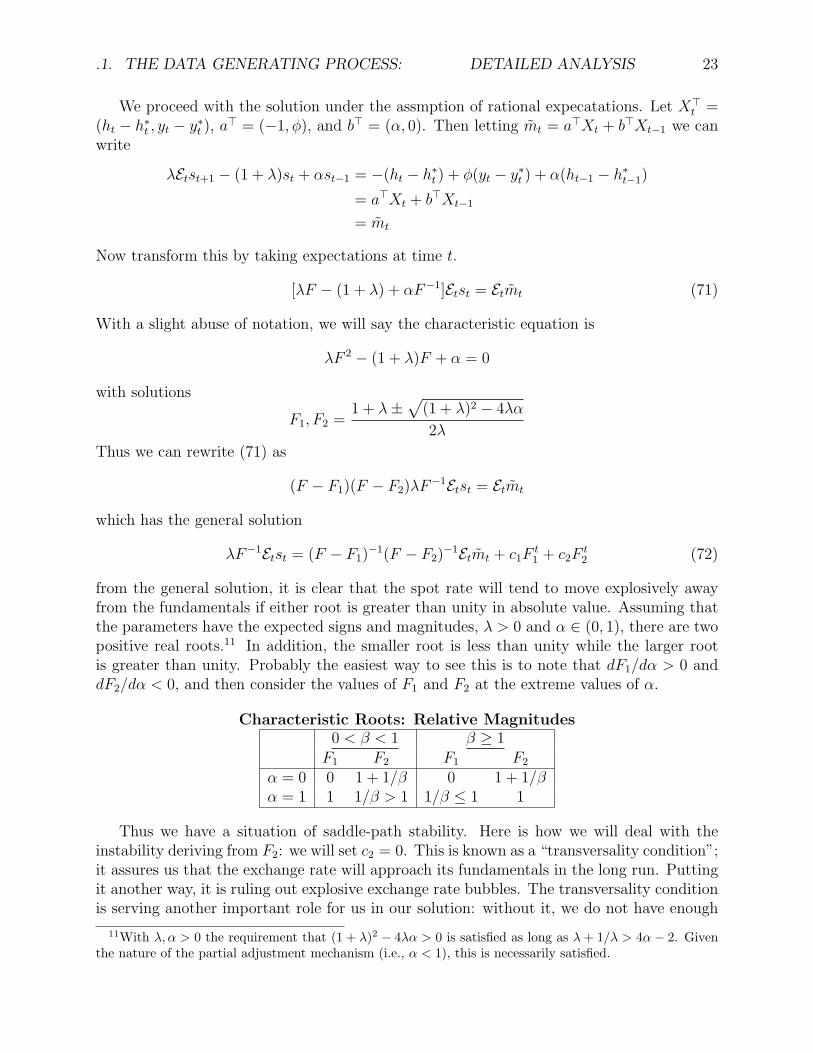
We proceed with the solution under the assmption of rational expecatations. Let X>t =(ht − h∗t , yt − y∗t ), a> = (−1, φ), and b> = (α, 0). Then letting mt = a>Xt + b>Xt−1 we canwrite

λEtst+1 − (1 + λ)st + αst−1 = −(ht − h∗t ) + φ(yt − y∗t ) + α(ht−1 − h∗t−1)

= a>Xt + b>Xt−1

= mt

Now transform this by taking expectations at time t.

[λF − (1 + λ) + αF−1]Etst = Etmt (71)

With a slight abuse of notation, we will say the characteristic equation is

λF 2 − (1 + λ)F + α = 0

with solutions

F1, F2 =1 + λ±

√(1 + λ)2 − 4λα

2λ

Thus we can rewrite (71) as

(F − F1)(F − F2)λF−1Etst = Etmt

which has the general solution

λF−1Etst = (F − F1)−1(F − F2)

−1Etmt + c1Ft1 + c2F

t2 (72)

from the general solution, it is clear that the spot rate will tend to move explosively awayfrom the fundamentals if either root is greater than unity in absolute value. Assuming thatthe parameters have the expected signs and magnitudes, λ > 0 and α ∈ (0, 1), there are twopositive real roots.11 In addition, the smaller root is less than unity while the larger rootis greater than unity. Probably the easiest way to see this is to note that dF1/dα > 0 anddF2/dα < 0, and then consider the values of F1 and F2 at the extreme values of α.

Characteristic Roots: Relative Magnitudes0 < β < 1 β ≥ 1F1 F2 F1 F2

α = 0 0 1 + 1/β 0 1 + 1/βα = 1 1 1/β > 1 1/β ≤ 1 1

Thus we have a situation of saddle-path stability. Here is how we will deal with theinstability deriving from F2: we will set c2 = 0. This is known as a “transversality condition”;it assures us that the exchange rate will approach its fundamentals in the long run. Puttingit another way, it is ruling out explosive exchange rate bubbles. The transversality conditionis serving another important role for us in our solution: without it, we do not have enough

11With λ, α > 0 the requirement that (1 + λ)2 − 4λα > 0 is satisfied as long as λ+ 1/λ > 4α− 2. Giventhe nature of the partial adjustment mechanism (i.e., α < 1), this is necessarily satisfied.

24 BIBLIOGRAPHY

information to determine a unique exchange rate. That is because we are working with asecond order difference equation, but we only have a single initial condition (st−1). We canhighlight the role of this initial condition by multiplying (72) by (F − F1).

(F − F1)λF−1Etst = (F − F2)

−1Etmt

Noting F1F2 = α/λ, we can write this as

(1− 1

F1

F )αF−1Etst = (1− 1

F2

F )−1Etmt

or, using summation notation,

Etst−1 −1

F1

Etst =1

α

∞∑i=0

(1

F2

)i

Etmt+i

Etst = F1Etst−1 −F1

α

∞∑i=0

(1

F2

)i

Etmt+i (73)

An Emprical Application

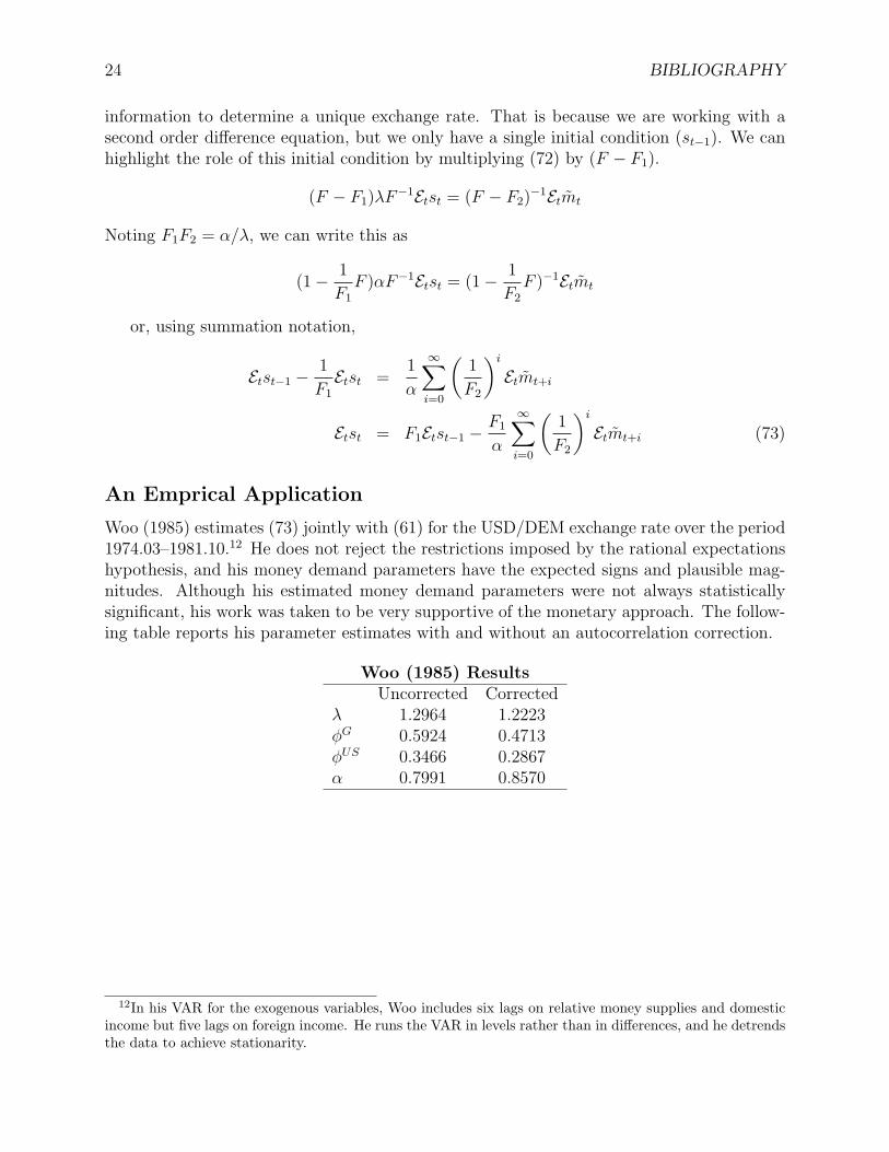
Woo (1985) estimates (73) jointly with (61) for the USD/DEM exchange rate over the period1974.03–1981.10.12 He does not reject the restrictions imposed by the rational expectationshypothesis, and his money demand parameters have the expected signs and plausible mag-nitudes. Although his estimated money demand parameters were not always statisticallysignificant, his work was taken to be very supportive of the monetary approach. The follow-ing table reports his parameter estimates with and without an autocorrelation correction.

Woo (1985) ResultsUncorrected Corrected

λ 1.2964 1.2223φG 0.5924 0.4713φUS 0.3466 0.2867α 0.7991 0.8570

12In his VAR for the exogenous variables, Woo includes six lags on relative money supplies and domesticincome but five lags on foreign income. He runs the VAR in levels rather than in differences, and he detrendsthe data to achieve stationarity.