1

Lecture Notes 3

1. Types of economic variables (i) Continuous variable – takes on a continuum in the sample space, such as all points on a line or all real numbers

Example: GDP, Pollution concentration, etc. (ii) Discrete variables – finite number of elements or an infinitely

countable number, such as all positive integers. Example: Number of workers, etc. (iii) Categorical data are grouped accordingly to some quality or

attribute Example: Sex or type of automobile.

2. Review of statistics (i) Population – the total group set of elements of interest.

Sample – a subset of the population. We usually collect samples because it is too costly to sample the entire population.

Example – College students’ survey in Kazakhstan Population is all college students

Probability – the relative frequency or occurrence of an event after repetitive trials or experiments.

Probability lies between 0 and 1 All probabilities for all events have to sum to 1 Example: 60% chance of rain today Implies a 40% of no rain, summing to one or 100%

2

(ii) Probability distribution functions (PDF) – a function that associates each value of a discrete random variable with the probability that this value will occur. Denoted as p(x) or f(x)

Cumulative probability distribution function (CDF) - integral of a probability function

Denoted by a capital letter, such as P(x) or F(x).

x

dttfxP

If you sum over all probabilities, then it has to equal one. 1

dttfxP

The normal probability distribution is shown below

3

(iii) Descriptive statistical measures – describe a sample or population.

Measures of central tendencies Mean – calculated by )x(fxx ii where f(x) is the pdf and x

is the random variable. This is also the expected value If every observation is equally likely, then ix

n1x where n

is the number of observations Median – the middle point or observation when the data are

ordered from smallest to largest. Mode – the value, which occurs most often in a distribution. The peak of a distribution Use calculus to find maximum value

Range – the difference between the largest value in the sample (the maximum) and the smallest value (the minimum),

minmax xxR

Variance – is a measure of deviation from the mean, denoted by 2

Variance has a problem If the units are in $’s, then variance is $2 The n-1 is the sample variance

Degrees of freedom (df) – the amount of information you have, i.e. the number of observations

Since you estimated the variance, you lose one piece of information

In regression, you have k parameters df = n – k, because you estimated k standard errors

4

1

)(ˆ 1

2

2

n

xxn

ii

where x denotes the mean of the sample

Standard deviation – the variability or spread of the data around its mean

Has same units of the variable (i.e. miles, dollars, kilometers, etc.).

2ˆˆ (iv) The Normal Distribution or Gaussian Distribution – the most

common distribution Bell-shaped curve Regression – you do not need a distribution to estimate parameters

However, if are testing the statistical significance of a parameter, then you need a distribution.

The top distribution is symmetric, thus the mean = median = mode

5

The bottom distributions are not symmetric, so emedianmean mod The Normal Distribution We have a relationship between probabilities and the mean and

standard deviation Write it as 2,~ xNxi

Statisticians have a trick to make all normal distributions standard,

which is 1,0~ Nz i Distribution is below:

6

The transformation is:

xxz i In the old days, people carried tables that had the probability for

particular z values. Excel can calculate this easily =normdist(z)

Note – this returns the probability from negative infinity to the z value

(v) Standard Error – the variability in the mean when taking

repeated samples The true parameter is unknown,

Each time I take a different sample from the population, I get a different estimate for the parameter

Example Mean of first sample is 23.5 Mean of second sample is 24.2 Mean of third sample is 22.9

nerrorstd .

Since I cannot keep taking samples, nor can I take observations of the whole population, I would like to know how my estimator varies.

ˆˆ n

n

z

Very similar to the z-transformation. I can use this relationship for hypothesis testing. Each hypotheses has two parts Null - is the hypothesis of interest, H0 Alternative - is the complement of the null, HA

7

A hypothesis has to incorporate all possible outcomes Example H0: = 4 HA: > 4 What about values below 4?

Properly stated null and alternative hypothesis cover all alternatives.

Example Two-tail test H0: = 0 HA: 0 This is very common Automatically computed for Linear Regression Does it appear the parameter equals zero? The x variable has no impact on the y Example Two-tail test H0: < 0 HA: 0 We have a problem, we do not know what the standard deviation is

and have to use a different distribution (vi) t-distribution – a symmetric bell-shaped distribution The problem is we do not know the parameter, Further, we do not know the standard deviation too, i.e. A little fatter and shorter than the standard bell curve The shape depends on degrees of freedom

8

Degrees of freedom is the amount of information, i.e. number of observations

We had to estimate the standard deviation, so we subtract 1 Regression – each parameter estimate has a standard error k parameters, thus, df = n – k

As the degrees of freedom approach infinity, the t-distribution approaches the standard normal distribution.

The t-test is

ˆ

ˆˆˆ

n

n

t

where hat is the variable of interest is the null hypothesis value

is a appropriate estimate of the standard deviation of x

n is the number of observations. Example – Homework #1 Does the data support that 2=2? We choose a level of significance, Usually = 0.05 Two-tail test H0: = -2 HA: -2 A two-tail test. Now calculate the degrees of freedom 60 observations and estimated two parameters df= 58 Find critical value for t value.

9

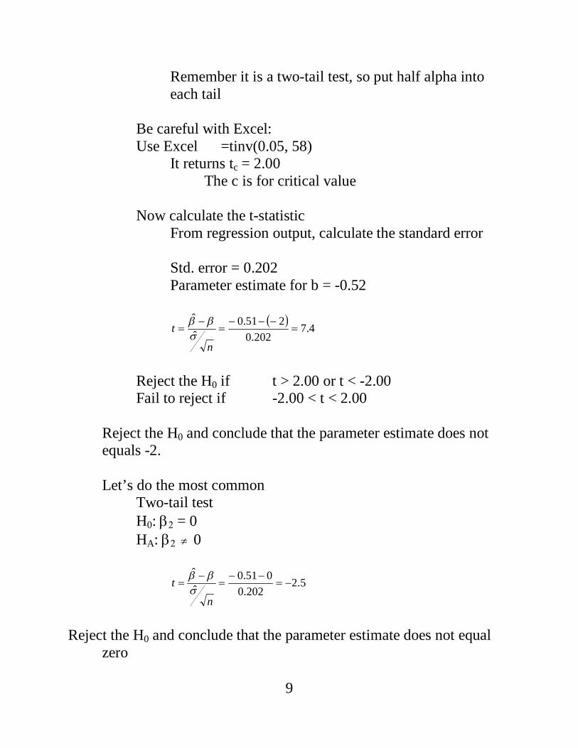
Remember it is a two-tail test, so put half alpha into each tail

Be careful with Excel: Use Excel =tinv(0.05, 58) It returns tc = 2.00 The c is for critical value Now calculate the t-statistic From regression output, calculate the standard error Std. error = 0.202 Parameter estimate for b = -0.52 4.7

202.0251.0

ˆˆ

n

t

Reject the H0 if t > 2.00 or t < -2.00 Fail to reject if -2.00 < t < 2.00

Reject the H0 and conclude that the parameter estimate does not equals -2.

Let’s do the most common Two-tail test H0: = 0 HA: 0 5.2

202.0051.0

ˆˆ

n

t

Reject the H0 and conclude that the parameter estimate does not equal

zero

10

Selected Critical Values for the t-distribution Level of Significance α - see diagrams above

Degrees of Freedom

.10 .05 .025 .01

1 3.078 6.314 12.706 63.657 15 1.341 1.753 2.131 2.947 19 1.328 1.729 2.093 2.861 20 1.325 1.725 2.086 2.845 21 1.323 1.323 2.080 2.518 ∞ 1.282 1.282 1.960 2.326

3. Analysis of Variance (ANOVA) In terms of regressions, ANOVA is used to test hypothesis in many types of statistical analysis Sum of Squared Total (SST) is defined as:

n

ii yySST

1

2)( .

yi is the dependent variable in the regression The yyi is the total variation for observation i

Sum of Squared Regression (SSR) is defined as:

n

1i

2i )yy(SSR .

This is the variation explained by the regression Sum of Squared Errors (SSE), which was earlier defined as: .ˆ.ˆ

1

2

1

2

n

ii

n

iii uyySSE

SSE is the amount of variation not explained by the regression equation.

Thus, SST = SSR + SSE, which is proved in the chapter

11

We can use this information to calculate the R2 statistic: SSTSSER 12

Show relationship:

SSTSSE

SSTSSRR

SSTSSE

SSTSSR

SSESSRSST

1

1

2

Problem – the more parameters added to the regression, the higher

the R2. R2 = 1, if n = k, the number of parameters equal observations Now we need the degrees of freedom for each measure: Sum of Squared Regression (SSR) df =k – 1 Sum of Squared Errors (SSE) df = n – k Sum of Squared Total (SST) df = n – 1 We calculate the Mean Square (MS) Regression (MS) = SSR / (k – 1) Residual (MS) =SSE / (n – k) Total (MS) NA Additional information When you have a variable with a normal distribution If you add or subtract if from other variables with a normal

distribution, then it is still normally distributed Calculating a mean is a first moment If you square a random variable with a normal distribution, then you get

a chi-square distribution with degrees of freedom. The squares are variances and called the second moment All the Mean Squares are distributed as chi squares

12

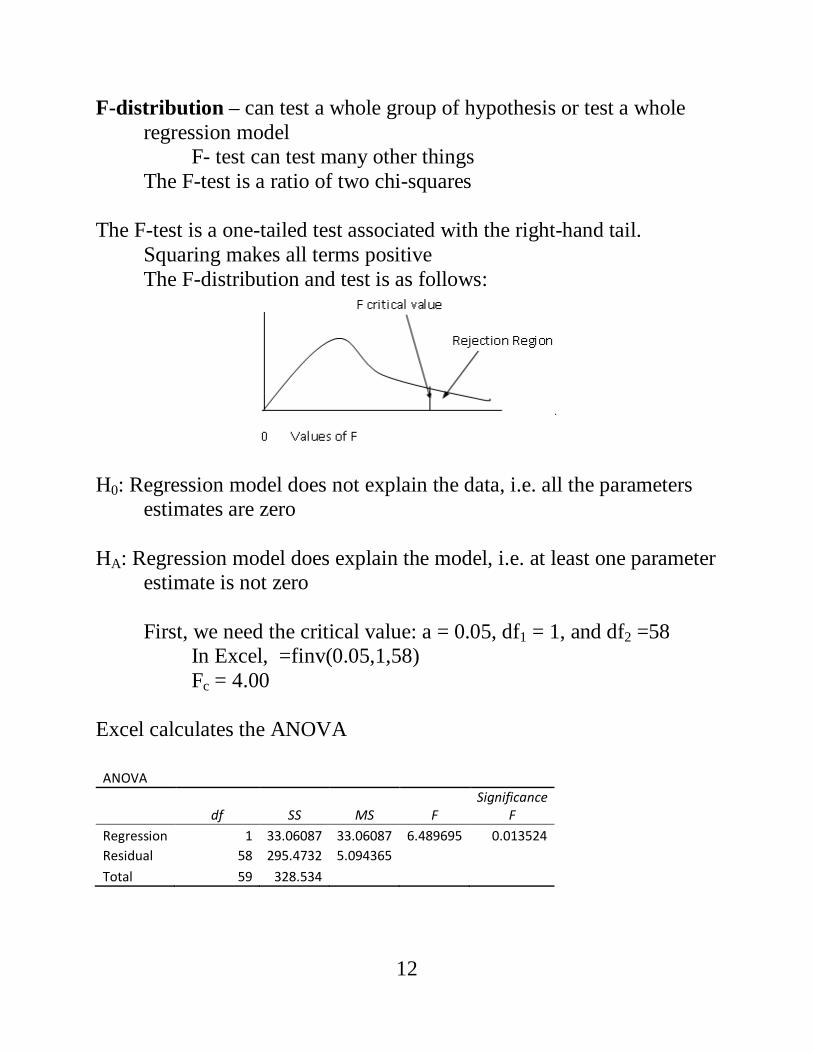
F-distribution – can test a whole group of hypothesis or test a whole regression model

F- test can test many other things The F-test is a ratio of two chi-squares The F-test is a one-tailed test associated with the right-hand tail. Squaring makes all terms positive The F-distribution and test is as follows:

H0: Regression model does not explain the data, i.e. all the parameters

estimates are zero HA: Regression model does explain the model, i.e. at least one parameter

estimate is not zero First, we need the critical value: a = 0.05, df1 = 1, and df2 =58 In Excel, =finv(0.05,1,58) Fc = 4.00 Excel calculates the ANOVA

ANOVA

df SS MS F Significance

F Regression 1 33.06087 33.06087 6.489695 0.013524 Residual 58 295.4732 5.094365 Total 59 328.534

13

Calculate the F-value = 50.609.506.33

5847.295

106.33

2

1 df

SSEdf

SSR

The computed F exceeds the Fc, so reject the H0, and conclude at least

one parameter is not equal to zero. Example from homework #3. How many observations? 10 How many parameters, k? 4 Degrees of freedom for error df = 10 – 4 = 6 Degrees of freedom for total df = 10 – 1 = 9 ANOVA

df SS MS F Significance

F Regression 3 5001.859635 1667.287 232.4265 1.35E-06 Residual 6 43.04036468 7.173394 Total 9 5044.9