lecture note 5, predicate logics
TRANSCRIPT

1
1
Predicate Calculus
Formal Methods
Lecture 5
Farn Wang
Dept. of Electrical Engineering
National Taiwan University
2
Predicate Logic
Invented by Gottlob
Frege (1848–1925).
Predicate Logic is also
called “first-order logic”.
“Every good mathematician is at least half a philosopher, and every good philosopher is at least half a mathematician.”

2
3
Motivation
There are some kinds of human reasoning that
we can‟t do in propositional logic.
For example:
Every person likes ice cream.
Billy is a person.
Therefore, Billy likes ice cream.
In propositional logic, the best we can do
is , which isn‟t a tautology.
We‟ve lost the internal structure.
A B C
4
Motivation
We need to be able to refer to objects.
We want to symbolize both a claim and the object
about which the claim is made.
We also need to refer to relations between objects,
as in “Waterloo is west of Toronto”.
If we can refer to objects, we also want to be able to
capture the meaning of every and some of.
The predicates and quantifiers of predicate logic
allow us to capture these concepts.

3
5
Apt-pet
An apartment pet is a pet
that is small
Dog is a pet
Cat is a pet
Elephant is a pet
Dogs and cats are small.
Some dogs are cute
Each dog hates some cat
Fido is a dog)(
),()()(
)()(
)()(
)()(
)()(
)()(
)()(
)()()(
fidodog
yxhatesycatyxdogx
xcutexdogx
xsmallxcatx
xsmallxdogx
xpetxelephantx
xpetxcatx
xpetxdogx
xaptPetxpetxsmallx
6
Universal quantification () corresponds to
finite or infinite conjunction of the application
of the predicate to all elements of the domain.
Existential quantification () corresponds to
finite or infinite disjunction of the application
of the predicate to all elements of the domain.
Relationship between and :
x.P(x) is the same as x. P(x)
x.P(x) is the same as x. P(x)
Quantifiers

4
7
Functions
Consider how to formalize:
Mary‟s father likes music
One possible way: x(f(x, Mary)Likes(x,Music))
which means: Mary has at least one father and he likes music.
We‟d like to capture the idea that Mary only has one father. We use functions to capture the single object that can be in
relation to another object.
Example: Likes(father(Mary),Music)
We can also have n-ary functions.
8
Predicate Logic
syntax (well-formed formulas)
semantics
proof theory
axiom systems
natural deduction
sequent calculus
resolution principle

5
9
Predicate Logic: Syntax
The syntax of predicate logic consists of:
constants
variables
functions
predicates
logical connectives
quantifiers
punctuations: , . ( )
, ,x y
10
Predicate Logic: Syntax
Definition. Terms are defined inductively as
follows:
Base cases
Every constant is a term.
Every variable is a term.
inductive cases
If t1,t2,t3,…,tn are terms then f(t1,t2,t3,…,tn) is a term,
where f is an n-ary function.
Nothing else is a term.

6
11
Predicate Logic
- syntax
Definition. Well-formed formulas (wffs) are defined inductively as follows:
Base cases: P(t1,t2,t3,…,tn) is a wff, where ti is a term, and P is an n-ary
predicate. These are called atomic formulas.
inductive cases: If A and B are wffs, then so are
A, AB, AB, AB, AB
If A is a wff, so is x. A
If A is a wff, so is x. A
Nothing else is a wff.
We often omit the brackets using the same precedence rules as propositional logic for the logical connectives.
12
Scope and Binding of Variables (I)
Variables occur both in nodes next to quantifiers
and as leaf nodes in the parse tree.
A variable x is bound if starting at the leaf of x,
we walk up the tree and run into a node with a
quantifier and x.
A variable x is free if starting at the leaf of x, we
walk up the tree and don‟t run into a node with a
quantifier and x.
.( .( ( ) ( ))) ( ( ) ( ))x x P x Q x P x Q y

7
13
Scope and Binding of Variables (I)
The scope of a variable x is the subtree starting at
the node with the variable and its quantifier
(where it is bound) minus any subtrees with or
at their root.
Example:
A wff is closed if it contains no free occurrences of
any variable.
x x
.( .( ( ) ( ))) ( ( ) ( ))x x P x Q x P x Q y
scope of this xscope of this x
14
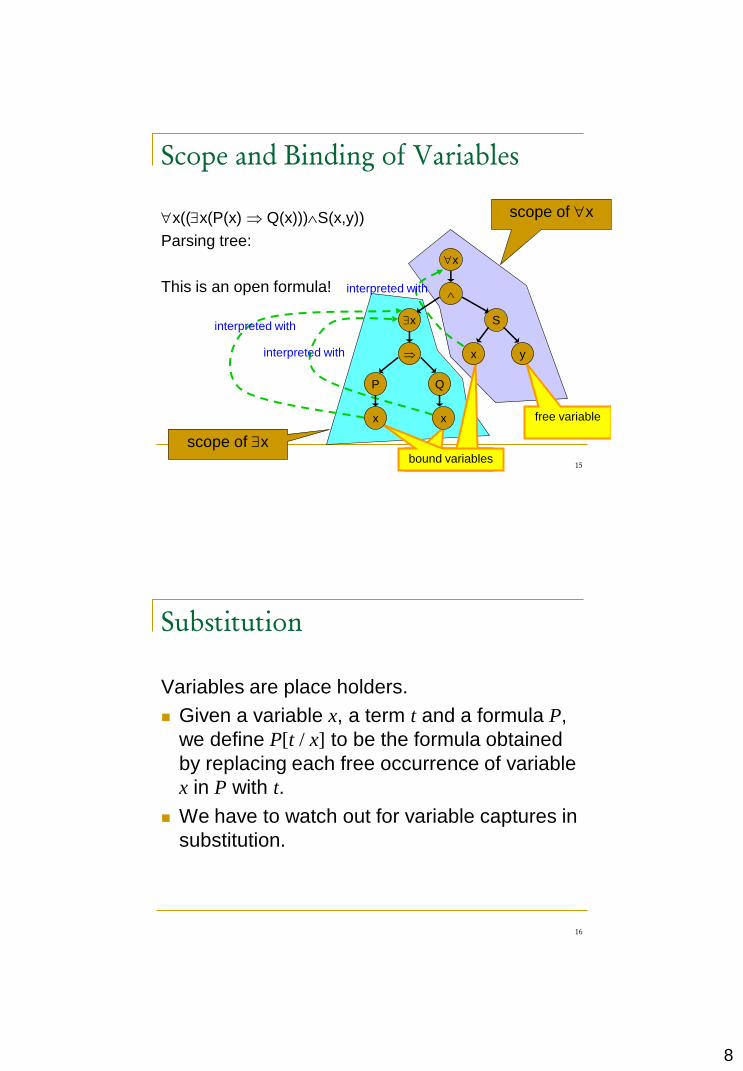
Scope and Binding of Variables
x((P(x) Q(x))S(x,y))
Parsing tree:
This is an open formula!
x
P Q
xx
S
yx
scope of x
interpreted with
interpreted with
interpreted with
bound variables
free variable
8
15
Scope and Binding of Variables
x((x(P(x) Q(x)))S(x,y))
Parsing tree:
This is an open formula!
scope of x
interpreted with
interpreted with
interpreted with
bound variables
free variable
x
x
P Q
xx
S
yx
scope of x
16
Substitution
Variables are place holders.
Given a variable x, a term t and a formula P,
we define P[t / x] to be the formula obtained
by replacing each free occurrence of variable
x in P with t.
We have to watch out for variable captures in
substitution.

9
17
Substitution
In order not to mess up with the meaning of the
original formula, we have the following restrictions
on substitution.
Given a term t, a variable x and a formula P,
“t is not free for x in P”
if
x in a scope of y or y in A; and
t contains a free variable y.
Substitution P[t / x] is allows only if t is free for x in P.
18
Substitution
Example:
y(mom(x)dad(f(y))) z(mom(x)dad(f(z)))
But
(y(mom(x)dad(y)))[f(y)/x] = y(mom(f(y))dad(f(y)))
(z(mom(x)dad(z)))[f(y)/x] = z(mom(f(y))dad(f(z)))
equivalent
[f(y)/x] not allowed since
meaning of formulas
messed up.

10
19
Predicate Logic: Semantics
Recall that a semantics is a mapping
between two worlds.
A model for predicate logic consists of:
a non-empty domain of objects:
a mapping, called an interpretation that associates
the terms of the syntax with objects in a domain
It‟s important that be non-empty,
otherwise some tautologies wouldn‟t hold
such as
ID
ID
( . ( )) ( . ( ))x A x x A x
20
Interpretations (Models)
a fixed element c’ DI to each constant c of
the syntax
an n-ary function f’:DIn DI to each n-ary
function, f, of the syntax
an n-ary relation R’ DIn to each n-ary
predicate, R, of the syntax

11
21
Example of a Model
Let‟s say our syntax has a constant c, a function f(unary), and two predicates P, and Q (both binary).
Example: P(c,f(c))
In our model, choose the domain to be the natural numbers
I(c) is 0.
I(f) is suc, the successor function.
I(P) is `<„
I(Q) is `=„
22
Example of an Model
What‟s the meaning of P(c,f(c)) in this model?
Which is true.
( ( , ( ))) ( ) ( ( ))
0 ( ( ))
0 (0)
0 1
I P c f c I c I f c
suc I c
suc
12
23
Valuations
Definition.
A valuation v, in an interpretation I, is a function
from the terms to the domain DI such that:
ν(c) = I(c)
ν(f(t1,…,tn)) = f’(ν(t1),…, ν (tn))
ν(x)DI, i.e., each variable is mapped onto
some element in DI
24
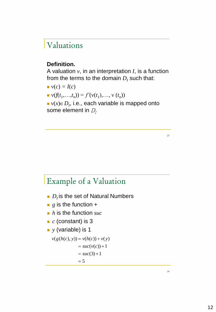
Example of a Valuation
DI is the set of Natural Numbers
g is the function +
h is the function suc
c (constant) is 3
y (variable) is 1
( ( ( ), )) ( ( )) ( )
( ( )) 1
(3) 1
5
v g h c y v h c v y
suc v c
suc

13
25
Workout
DI is the set of Natural Numbers
g is the function +
h is the function suc
c (constant) is 3
y (variable) is 1
ν(h(h(g(h(y),g(h(y),h(c)))))) = ?
26
False
True
True
True
On(A,B)
Clear(B)
On(C,Fl)
On(C,Fl) On(A,B)

14
27
Workout
Interpret the following formulas with respect to
the world (model) in the previous page.
On(A,Fl) Clear(B)
Clear(B) Clear(C) On(A,Fl)
Clear(B) Clear(A)
Clear(B)
Clear(C)
B
C
A
28
Konwoledge
Does the following knowledge base (set of
formulae) have a model ?
On(A,Fl) Clear(B)
Clear(B) Clear(C) On(A,Fl)
Clear(B) Clear(A)
Clear(B)
Clear(C)
15
29
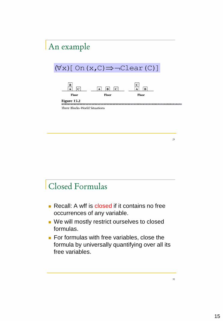
An example
( x)[On(x,C) Clear(C)]
30
Closed Formulas
Recall: A wff is closed if it contains no free
occurrences of any variable.
We will mostly restrict ourselves to closed
formulas.
For formulas with free variables, close the
formula by universally quantifying over all its
free variables.

16
31
Validity (Tautologies)
Definition. A predicate logic formula is satisfiable if there is an interpretation and there is a valuation that satisfies the formula (i.e., in which the formula returns T).
Definition. A predicate logic formula is logically valid (tautology) if it is true in every interpretation. It must be satisfied by every valuation in every
interpretation.
Definition. A wff, A, of predicate logic is a contradiction if it is false in every interpretation. It must be false in every valuation in every interpretation.
32
Satisfiability, Tautologies,
Contradictions
A closed predicate logic formula, is satisfiable
if there is an interpretation I in which the
formula returns true.
A closed predicate logic formula, A, is a
tautology if it is true in every interpretation.
A
A closed predicate logic formula is a
contradiction if it is false in every
interpretation.

17
33
Tautologies
How can we check if a formula is a tautology?
If the domain is finite, then we can try all the possible interpretations (all the possible functions and predicates).
But if the domain is infinite? Intuitively, this is why a computer cannot be programmed to determine if an arbitrary formula in predicate logic is a tautology (for all tautologies).
Our only alternative is proof procedures!
Therefore the soundness and completeness of our proof procedures is very important!
34
Semantic Entailment
Semantic entailment has the same meaning as
it did for propositional logic.
means that if and and
then , which is equivalent to saying
is a tautology, i.e.,
1 2 3, ,
1( ) Tv 2( ) Tv 3( ) Tv
( ) Tv
1 2 3( )
1 2 3 1 2 3( , , ) (( ) )

18
35
An Axiomatic System for Predicate
Logic
FO_AL: An extension of the axiomatic system for
propositional logic. Use only:
where A contains
no free occurrences of x
. .
( )
( ( )) (( ) ( ))
( ) ( )
. ( ) ( ), where is free for in
.( ) ( ( . )),
A B A
A B C A B A C
A B B A
x A x A t t x A
x A B A x B
36
FO_AL Rules of Inference
Two rules of inference:
(modus ponens - MP) From A and , B
can be derived, where A and B are any well-
formed formulas.
(generalization) From A, can be derived,
where A is any well-formed formula and x is
any variable.
A B
.x A

19
37
Soundness and Completeness of
FO_AL
FO_AL is sound and complete.
Completeness was proven by Kurt Gödel in
1929 in his doctoral dissertation.
Predicate logic is not decidable
38
Deduction Theorem
Theorem. If by a deduction
containing no application of generalization to
a variable that occurs free in A, then
Corollary. If A is closed and if then
{ }ph
H A B
phH A B
{ }ph
H A B
( )ph
H A B
20
39
A closed formula is a tautology (valid) iff its
negation is a contradiction.
In other words, A closed formula is valid iff its
negation is not satisfiable.
To prove {P1,…, Pn} ⊨ S is equivalent to
prove {P1,…, Pn, ¬S} ⊨ false
To prove {P1,…, Pn} ⊨ S becomes to check
if there is an interpretation for {P1,…, Pn,
¬S} .
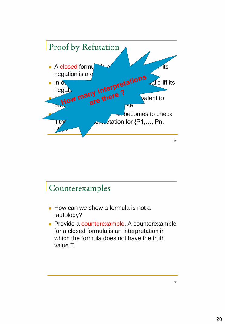
Proof by Refutation
40
Counterexamples
How can we show a formula is not a
tautology?
Provide a counterexample. A counterexample
for a closed formula is an interpretation in
which the formula does not have the truth
value T.
21
41
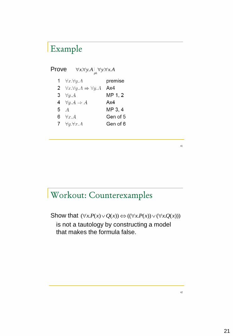
Example
Prove . . . .ph
x y A y x A
42
Workout: Counterexamples
Show that
is not a tautology by constructing a model
that makes the formula false.
( . ( ) ( )) (( . ( )) ( . ( )))x P x Q x x P x x Q x

22
43
What does „first-order‟ mean?
We can only quantify over variables.
In higher-order logics, we can quantify over
functions, and predicates.
For example, in second-order logic, we can
express the induction principle:
Propositional logic can also be thought of as
zero-order.
.( (0) ( . ( ) ( 1))) ( . ( ))P P n P n P n n P n
44
A rough timeline in ATP … (1/3)
450B.C. Stoics propositional logic (PL),
inference (maybe)
322B.C. Aristotle ``syllogisms“ (inference rules),
quantifiers
1565 Cardano probability theory (PL + undertainty)
1646 Leibniz research for a general decision procedure
-1716 to check the validty of formulas
1847 Boole PL (again)
1879 Frege first-order logic (FOL)
1889 Peano 9 axioms for natural numbers

23
45
A rough timeline in ATP … (2/3)
1920‘s Hilbert Hilbert‘s program
1922 Wittgenstein proof by truth tables
1929 Gödel completeness theorem of FOL
1930 Herbrand a proof procedure for FOL based on
propositionalization
1931 Gödel incompleteness theorems for the consistency
of Peano axioms
1936 Gentzen a proof for the consisitency of Peano axioms
in set theory
1936 Church, undecidability
Turing of FOL
1958 Gödel a method to prove the consistency of Peano
axioms with type theory
• To formalize all existing
theories to a finite,
complete, and
consistent set of axioms.
• decision procedures for
all mathematical
theories
• 23 open problems.
Resolve the
2nd Hilbert‟s
problem (in
the theory of
N)
Who is to
prove the
consistency
of set theory ?
Is type
theory
consistent
?
46
A rough timeline in ATP … (3/3)
1954 Davis First machine-generated proof
1955 Beth, Semantic Tableaus
Hintikka
1957 Newell, First machine-generated proof in
Simon Logic Calculus
1957 Kangar, Lazy substitution by free (dummy) Vars
Prawitz
1958 Prawitz First prover for FOL
1959 Gilmore More provers
Wang
1960 Davis Davis-Putnam Procedure
Putnam,
Longman
1963 Robinson Unification, resolution

24
47
Kurt Gödel
1906-1978
• Born an Austro-Hugarian
• 12 Czech
• refuse to learn Czech
• 23 Austrian
• established the completeness of
1st-order logic in his Ph.D. thesis
• 25, established the incompleteness of
• 32 German
• 34 joined Princeton
• 42 American
• Einstein, “his work no longer meant
much, that he came to the Institute
merely … to have the privilege of
walking home with Gödel.”
• On his citizen exam, …
• proved a paradoxial solution to the
general relativity
• Permanent position, Princeton, 1946
• 1st Albert Einstein Award, 1951
• Full professor, 1953
• National Science Medal, 1974
• Emeritus professor, 1976
American is in danger
of dictatorship because
I can prove the
contradiction in
American constitution.
• thought someone was to poison
him.
• ate only his wife‟s cooking.
• 1977, his wife was ill and could
not cook.
• Jan. 1978, died of mal-nutrition.
I knew the
general
relativity
was wrong.
48
2007/04/03 stopped here.

25
49
Predicate Logic: Natural Deduction
Extend the set of rules we used for
propositional logic with ones to handle
quantifiers.
50
Predicate Logic: Natural Deduction

26
51
Example
Show . ( ) ( ), . ( ) . ( )ND
x P x Q x x P x x Q x
52
Workout
Show
Show
( ), . ( ) ( ) ( )ND
P a x P x Q x Q a
. ( ) . ( )ND
x P x x P x

27
53
To prove {P1,…, Pn} ⊨ S is equivalent to
prove that there is no interpretation for
{P1,…, Pn, ¬S} .
But there are infinitely many interpretations!
Can we limit the range of interpretations ?
Yes, Herbrand interpretations!
Proof by Refutation
54
Herbrand‟s theorem
- Herbrand universe of a formula S
Let H0 be the set of constants appearing in S.
If no constant appears in S, then H0 is to consist of a
single constant, H0={a}.
For i=0,1,2,…
Hi+1=Hi {f n(t1,…,tn)| f is an n-place function in S; t1,…,tn Hi }
Hi is called the i-level constant set of S.
H is the Herbrand universe of S.

28
55
Herbrand‟s theorem
- Herbrand universe of a formula S
Example 1: S={P(a),P(x)P(f(x))}
H0={a}
H1={a,f(a)}
H2={a,f(a),f(f(a))}
.
.
H={a,f(a),f(f(a)),f(f(f(a))),…}
56
Herbrand‟s theorem
- Herbrand universe of a formula S
Example 2: S={P(x)Q(x),R(z),T(y)W(y)}
There is no constant in S, so we let H0={a}
There is no function symbol in S, henceH=H0=H1=…={a}
Example 3: S={P(f(x),a,g(y),b)}
H0={a,b}
H1={a,b,f(a),f(b),g(a),g(b)}
H2={a,b,f(a),f(b),g(a),g(b),f(f(a)),f(f(b)),f(g(a)),f(g(b)),g(f(a)),g(f(b)),g(g(a)),g(g(b))}
…

29
57
Herbrand‟s theorem
- Herbrand universe of a formula S
Expression a term, a set of terms, an atom, a set of atoms, a
literal, a clause, or a set of clauses.
Ground expressions expressions without variables.
It is possible to use a ground term, a ground atom, a ground literal, and a ground clause –this means that no variable occurs in respective expressions.
Subexpression of an expression E an expression that occurs in E.
58
Herbrand‟s theorem
- Herbrand base of a formula S
Ground atoms Pn(t1,…,tn)
Pn is an n-place predicate occurring in S,
t1,…,tn H
Herbrand base of S (atom set)
the set of all ground atoms of S
Ground instance of S
obtained by replacing variables in S by members of
the Herbrand universe of S.

30
59
Herbrand‟s theorem
- Herbrand universe & base of a formula S
Example
S={P(x),Q(f(y))R(y)}
C=P(x) is a clause in S
H={a,f(a),f(f(a)),…} is the Herbrand universe of
S.
P(a), Q(f(a)), Q(a), R(a), R(f(f(a))), and
P(f(f(a))) are ground atoms of C.
60
Workout
{P(x), Q(g(x,y),a)R(f(x))}
please construct the set of ground terms
please construct the set of ground atoms
31
61
Herbrand‟s theorem
- Herbrand interpretation of a formula S
S, a set of clauses.
i.e., a conjunction of the clauses
H, the Herbrand universe of S and
H-interpretation I of S
I maps all constants in S to themselves.
Forall n-place function symbol f and h1,…,hn
elements of H,
I (f (h1,…,hn) ) = f(h1,…,hn)
62
Herbrand‟s theorem
- Herbrand interpretation of a formula S
There is no restriction on the assignment to
each n-place predicate symbol in S.
Let A={A1,A2,…,An,…} be the atom set of S.
An H-interpretation I can be conveniently
represented as a subset of A.
If Aj I, then Aj is assigned “true”,
otherwise Aj is assigned “false”.
32
63
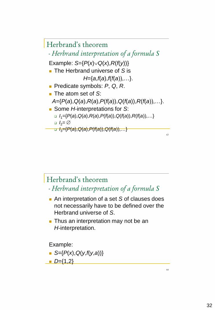
Herbrand‟s theorem
- Herbrand interpretation of a formula S
Example: S={P(x)Q(x),R(f(y))}
The Herbrand universe of S is
H={a,f(a),f(f(a)),…}.
Predicate symbols: P, Q, R.
The atom set of S:
A={P(a),Q(a),R(a),P(f(a)),Q(f(a)),R(f(a)),…}.
Some H-interpretations for S: I1={P(a),Q(a),R(a),P(f(a)),Q(f(a)),R(f(a)),…}
I2=
I3={P(a),Q(a),P(f(a)),Q(f(a)),…}
64
Herbrand‟s theorem
- Herbrand interpretation of a formula S
An interpretation of a set S of clauses does
not necessarily have to be defined over the
Herbrand universe of S.
Thus an interpretation may not be an
H-interpretation.
Example:
S={P(x),Q(y,f(y,a))}
D={1,2}
33
65
Herbrand‟s theorem
- Herbrand interpretation of a formula S
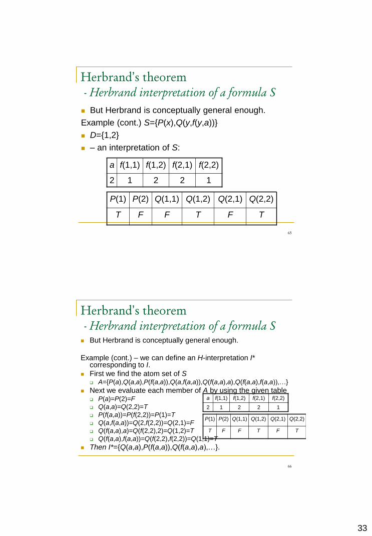
But Herbrand is conceptually general enough.
Example (cont.) S={P(x),Q(y,f(y,a))}
D={1,2}
– an interpretation of S:
a f(1,1) f(1,2) f(2,1) f(2,2)
2 1 2 2 1
P(1) P(2) Q(1,1) Q(1,2) Q(2,1) Q(2,2)
T F F T F T
66
Herbrand‟s theorem
- Herbrand interpretation of a formula S
But Herbrand is conceptually general enough.
Example (cont.) – we can define an H-interpretation I* corresponding to I.
First we find the atom set of S A={P(a),Q(a,a),P(f(a,a)),Q(a,f(a,a)),Q(f(a,a),a),Q(f(a,a),f(a,a)),…}
Next we evaluate each member of A by using the given table P(a)=P(2)=F
Q(a,a)=Q(2,2)=T
P(f(a,a))=P(f(2,2))=P(1)=T
Q(a,f(a,a))=Q(2,f(2,2))=Q(2,1)=F
Q(f(a,a),a)=Q(f(2,2),2)=Q(1,2)=T
Q(f(a,a),f(a,a))=Q(f(2,2),f(2,2))=Q(1,1)=T
Then I*={Q(a,a),P(f(a,a)),Q(f(a,a),a),…}.
a f(1,1) f(1,2) f(2,1) f(2,2)
2 1 2 2 1
P(1) P(2) Q(1,1) Q(1,2) Q(2,1) Q(2,2)
T F F T F T
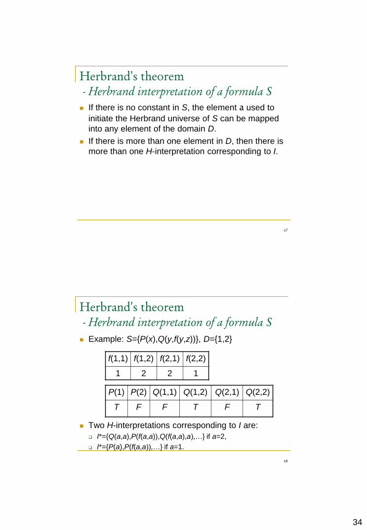
34
67
Herbrand‟s theorem
- Herbrand interpretation of a formula S
If there is no constant in S, the element a used to
initiate the Herbrand universe of S can be mapped
into any element of the domain D.
If there is more than one element in D, then there is
more than one H-interpretation corresponding to I.
68
Herbrand‟s theorem
- Herbrand interpretation of a formula S
Example: S={P(x),Q(y,f(y,z))}, D={1,2}
Two H-interpretations corresponding to I are:
I*={Q(a,a),P(f(a,a)),Q(f(a,a),a),…} if a=2,
I*={P(a),P(f(a,a)),…} if a=1.
f(1,1) f(1,2) f(2,1) f(2,2)
1 2 2 1
P(1) P(2) Q(1,1) Q(1,2) Q(2,1) Q(2,2)
T F F T F T

35
69
Herbrand‟s theorem
- Herbrand interpretation of a formula S
Definition: Given an interpretation I over a domain D, an H-interpretation I* corresponding to I is an H-interpretation that satisfies the condition:
Let h1,…,hn be elements of H (the Herbrand universe of S).
Let every hi be mapped to some di in D.
If P(d1,…,dn) is assigned T (F) by I, then P(h1,…,hn) is also assigned T(F) in I*.
Lemma: If an interpretation I over some domain Dsatisfies a set S of clauses, then any H-interpretation I* corresponding to I also satisfies S.
70
Herbrand‟s theorem
A set S of clauses is unsatisfiable if and only if S is
false under all the H-interpretations of S.
We need consider only H-interpretations for
checking whether or not a set of clauses is
unsatisfiable.
Thus, whenever the term “interpretation” is used, a
H-interpretation is meant.

36
71
Herbrand‟s theorem
Let denote an empty set. Then:
A ground instance C‟ of a clause C is satisfied by an
interpretation I if and only if there is a ground literal L‟ in C‟
such that L‟ is also in I, i.e. C‟I.
A clause C is satisfied by an interpretation I if and only if
every ground instance of C is satisfied by I.
A clause C is falsified by an interpretation I if and only if there
is at least one ground instance C‟ of C such that C‟ is not
satisfied by I.
A set S of clauses is unsatisfiable if and only if for every
interpretation I there is at least one ground instance C‟ of
some clause C in S such that C‟ is not satisfied by I.
72
Herbrand‟s theorem
Example: Consider the clause C=P(x)Q(f(x)). Let I1, I2, and I3 be defined as follows:
I1=
I2={P(a),Q(a),P(f(a)),Q(f(a)),P(f(f(a))),Q(f(f(a))),…}
I3={P(a),P(f(a)),P(f(f(a))),…}
C is satisfied by I1 and I2, but falsified by I3.
Example: S={P(x),P(a)}.
The only two H-interpretations are:
I1={P(a)},
I2= .
S is falsified by both H-interpretations and therefore is unsatisfiable.

37
73
Resolution Principle
- Clausal Forms
Clauses are universally quantified disjunctions
of literals;
all variables in a clause are universally
quantified1 1
1
1
( ,..., )( ... )
written as
...
or
{ ,..., }
n n
n
n
x x l l
l l
l l
74
Resolution Principle
- Clausal forms
Examples:
We need to be able to work with variables !
Unification of two expressions/literals
gives
{Nat(s(A)), Nat(A)}
{Nat(A)}
{Nat(s(A))}
gives
{Nat(s(s(x))), Nat(s(x))}
{Nat(s(A))}
{Nat(s(s(A)))}
gives
{Nat(s(A)), Nat(A)}
{Nat(x)}
{Nat(s(A))}

38
75
Resolution Principle
- Terms and instances
Consider following atoms
Ground expressions do not contain any variables
alphabetic variant
instance
instance
not an instance
P(x,f(y),B)
P(z,f(w),B)
P(x,f(A),B)
P(g(z),f(A),B)
P(C,f(A),A)
76
Resolution Principle
- Substitution
1 1A substitution { / ,..., / } substitutes
variables for terms ( does NOT contain )
Applying a substitution to an expression
yields the expression which is
with all occurrences of
n n
i i i i
s t v t v
v t t v
s
s
replaced by i iv t
no substitution !
P(x,f(y),B)
P(z,f(w),B) s={z/x,w/y}
P(x,f(A),B) s={A/y}
P(g(z),f(A),B) s={g(z)/x,A/y}
P(C,f(A),A)

39
77
Workout
Calculate the substitutions for the resolution of
the two clauses and the result clauses after
the substitutions.
P(x), P(f(a))Q(f(y),g(a,b))
P(g(x,a)), P(y)Q(f(y),g(a,b))
P(g(x,f(a))), P(g(b,y))Q(f(y),g(a,b))
P(g(f(x),x)), P(g(y,f(f(y)))Q(f(y),g(a,b)))
78
Resolution Principle
- Composing substitutions
Composing substitutions s1 and s2 gives s1 s2
which is that substitution obtained by first applying s2 to the terms in s1and adding remaining term/vars pairs to s1
Apply to
={g(x,y)/z}{A/x,B/y,C/w,D/z}=
{g(A,B)/z,A/x,B/y,C/w}
P(x,y,z)
gives
P(A,B,g(A,B))
40
79
Resolution Principle
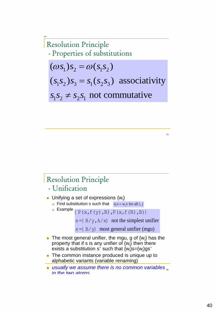
- Properties of substitutions
s
1 2 1 2
1 2 3 1 2 3
1 2 2 1
( ) ( )
( ) ( ) associativity
not commutative
s s s s
s s s s s s
s s s s
80
Resolution Principle
- Unification
Unifying a set of expressions {wi} Find substitution s such that
Example
The most general unifier, the mgu, g of {wi} has the property that if s is any unifier of {wi} then there exists a substitution s’ such that {wi}s={wi}gs’
The common instance produced is unique up to alphabetic variants (variable renaming)
usually we assume there is no common variables in the two atoms.
for all ,i jw s w s i j
not the simplest unifier
most general unifier (mgu)
{P(x,f(y),B),P(x,f(B),B)}
s={B/y,A/x}
s={B/y}

41
81
Workout
P(B,f(x),g(A)) and P(y,z,f(w))
construct an mgu
construct a unifier that is not the most general.
82
Workout
Determine if each of the following sets is
unifiable. If yes, construct an mgu.
{Q(a), Q(b)}
{Q(a,x),Q(a,a)}
{Q(a,x,f(x)),Q(a,y,y)}
{Q(x,y,z),Q(u,h(v,v),u)}
{P(x1,g(x1),x2,h(x1,x2),x3,k(x1,x2,x3)),
P(y1,y2,e(y2),y3,f(y2,y3),y4)}

42
83
Resolution Principle
- Disagreement set in unification
The disagreement set of a set of expressions
{wi} is the set of subterms { ti } of {wi} at the
first position in {wi} for which the {wi} disagree
gives
gives
gives
{P(x,A,f(y)),P(w,B,z)} {x,w}
{P(x,A,f(y)),P(x,B,z)} {A,B}
{P(x,y,f(y)),P(x,B,z)} {y,B}
84
Resolution Principle
- Unification algorithm
Unify( )
Initialize 0;
Initialize ;
Initialize {};
* If is a singleton, then output . Otherwise, continue.
Let be the disagreement set of
If there exists a var and a term
k
k
k k
k k
k k
Terms
k
T Terms
T
D T
v t
1
1
in D such that
does not occur in , continue. Otherwise, exit with failure.
{ / };
{ / };
1;
Goto *
k k
k
k k k k
k k k k
v
t
t v
T T t v
k k
43
85
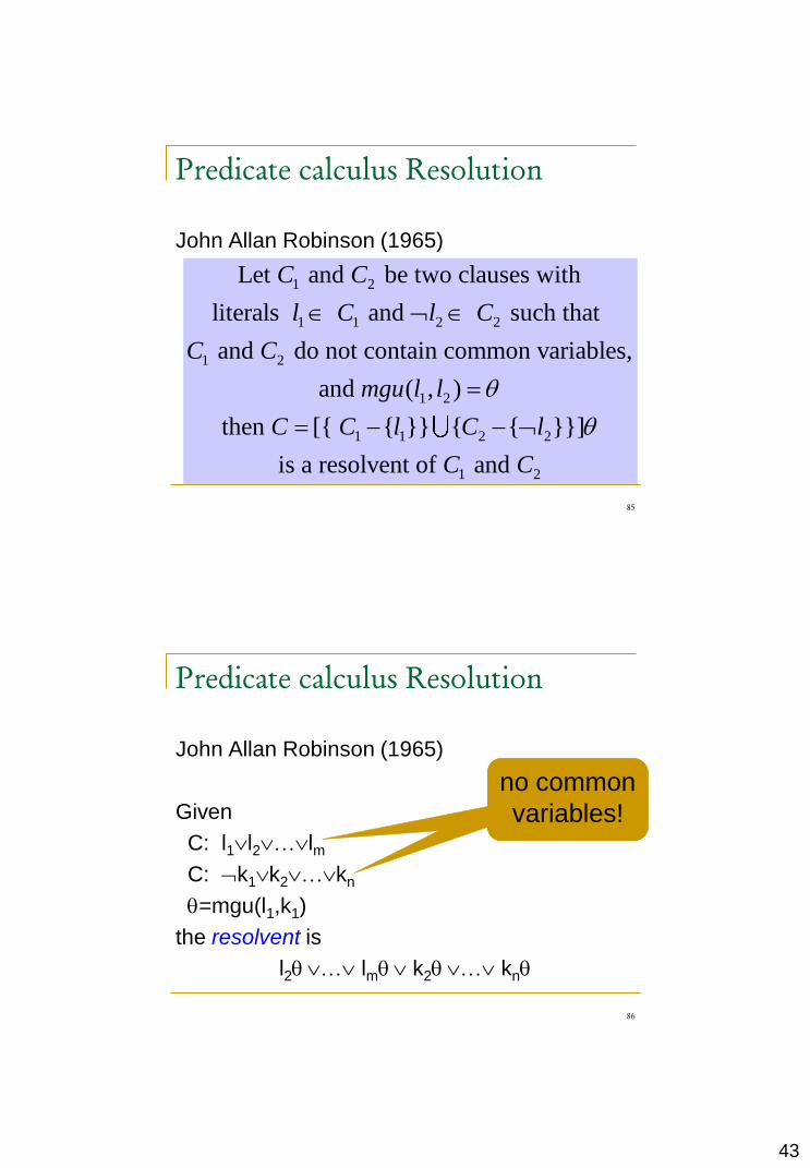
Predicate calculus Resolution
John Allan Robinson (1965)
1 2
1 1 2 2
1 2
1 2
1 1 2 2
1 2
Let and be two clauses with
literals and such that
and do not contain common variables,
and ( , )
then [{ { }} { { }}]
is a resolvent of and
C C
l C l C
C C
mgu l l
C C l C l
C C
86
John Allan Robinson (1965)
Given
C: l1l2…lm
C: k1k2…kn
=mgu(l1,k1)
the resolvent is
l2 … lm k2 … kn
Predicate calculus Resolution
no common
variables!

44
87
Resolution Principle
- Exampleand
Standardizing the variables apart
and
Substitution =
Resolvent
P(x) Q(f(x)) R(g(x)) Q(f(A))
P(x) Q(f(x)) R(g(y)) Q(f(A))
{A/x}
P(A) R(g(y))
and
Standardizing the variables apart
Substitution =
Resolvent
P(x) Q(x,y) P(A) R(B,z)
{A/x}
Q(A,y) R(B,z)
Why
can we
do this ?
Why we
think the
variables in
2 clauses
are
irrelevant ?
88
Workout
Find all the possible resolvents (if any) of the
following pairs of clauses.
P(x)Q(x,b),

45
89
Workout
Find all the possible resolvents (if any) of the
following pairs of clauses.
P(x)Q(x,b), P(a)Q(a,b)
P(x)Q(x,x), Q(a,f(a))
P(x,y,u)P(y,z,v)P(x,v,w)P(u,z,w),
P(g(x,y),x,y)
P(v,z,v)P(w,z,w), P(w,h(x,x),w)
90
Resolution Principle
- A stronger version of resolution
Use more than one literal per clause
and
do not resolve to empty clause.
However, ground instances
and resolve to empty clause
{P(u),P(v)} { P(x), P(y)}
{P(A)} { P(A)}

46
91
Resolution Principle
- Factors
1
1. 1 1
Let be a clause such that there exists
a substitution that is a mgu of a set of literals
in Then is a factor of
Each clause is a factor of itself.
Also, {P(f(y)),R(f(y),y)}is a factor of {P(x
C
C C C
),P(f(y)),R(x,y)}
with { ( ) / }f y x
92
Resolution Principle
- Example of refutation

47
93
Resolution Principle
- Example
Hypothesiesx (dog(x) animal(x))
dog(fido)
y (animal(y) die(y))
Conclusion
die(fido)
Clausal Form¬dog(x) animal(x)
dog(fido)
¬animal(y) die(y)
Negate the goal
¬die(fido)
94
Resolution Principle
- Example ¬dog(x) animal(x) ¬animal(y) die(y)
¬dog(y) die(y)
{x {x → y}
dog(fido)
die(fido)
{y → fido}
¬die(fido)

48
95
Workout (resolution)
- Proof with resolution principle
Hypotheses:
P(m(x),x) Q(m(x))
P(y,z) R(y)
Q(m(f(x,y))) T(x,g(y))
S(a) T(f(a),g(x))
R(m(y))
S(x) W(x,f(x,y))
Conclusion
W(a, y)
96
Resolution
Properties
Resolution is sound
Incomplete
But fortunately it is refutation complete If KB is unsatisfiable then KB |-
Given
Infer
P(A)
{P(A),P(B)}

49
97
Resolution Principle
- Refutation Completeness
To decide whether a formula KB ⊨ w, do
Convert KB to clausal form KB’
Convert w to clausal form w’
Combine w’ and KB’ to give Iteratively apply resolution to and add the
results back to until either no more resolvents can be added, or until the empty clause is produced.
98
Resolution Principle
- Converting to clausal form (1/2)
To convert a formula KB into clausal form
1. Eliminate implication signs*
2. Reduce scope of negation signs*
3. Standardize variables
4. Eliminate existential quantifiers using Skolemization
* Same as in prop. logic
( ) becomes ( )p q p q
( ) becomes ( )p q p q
( becomes ( x)[ P(x) ( x)Q(x)] x)[ P(x) ( y)Q(y)]
50
99
Resolution Principle
- Converting to clausal form (2/2)
5. Convert to prenex form
Move all universal quantifiers to the front
6. Put the matrix in conjunctive normal form*
Use distribution rule
7. Eliminate universal quantifiers
8. Eliminate conjunction symbol *
9. Rename variables so that no variable occurs in
more than one clause.
100
Resolution Principle
- Skolemization
General rule is that each occurrence of an existentially
quantified variable is replaced by a skolem function whose
arguments are those universally quantified variables
whose scopes includes the scope of the existentially
quantified one
Skolem functions do not yet occur elsewhere !
Resulting formula is not logically equivalent !
Consider
The depends on the
Define this dependence e skolem function xplicitly using a
Formula becomes
h
( x)[( y)Height(x,y)]
y x
( x)[Height(x,h(
(x)
x))]

51
101
Resolution Principle
- Examples of Skolemization
A well formed formula and its Skolem form are not logically equivalent.
However, a set of formulae is (un)satisfiable if and only if its skolem form is (un)satisfiable.
gives
[( w)Q(w)] ( x){( y){( z)[P(x,y,z) ( u)R(x,y,u,z)]}}
[( w)Q(w)] ( x){( y)[P(x,y,g(x,y)) ( u)R(x,y,u,g(x,y))]}
( gives (
but
( gi
Not logically equivalent
ves skolem constant
!
x)[( y) F(x,y)] x)F(x,
y) [( x)F(x,y)] [( x)F(x, )]
)
sk
h(x )
102
Resolution Principle
- Example of conversion to clausal form

52
103
Workout
Convert the following formula to clausal form.
x(P(x)y
((z.Q(x,y,s(z)))(Q(x,s(y),x)R(y))))
xy(S(x,y,z) z(S(x,z) S(z,x)))
104
Resolution Principle
- Example of refutation by resolution
all packages in room 27 are smaller than any of those in 28
Prove
1. P(x) P(y) I(x,27) I(y,28) S(x,y)
2.P(A)
3.P(B)
4.I(A,27) I(A,28)
5.I(B,27)
6. S(B,A)
I(A,27)

53
105
Resolution Principle
- Search Strategies
Ordering strategies In what order to perform resolution ?
Breadth-first, depth-first, iterative deepening ?
Unit-preference strategy : Prefer those resolution steps in which at least one
clause is a unit clause (containing a single literal)
Refinement strategies Unit resolution : allow only resolution with unit
clauses
106
Resolution Principle
- Input Resolution
at least one of the clauses being resolved is a member of the original set of clauses
Input resolution is complete for Horn-clauses but incomplete in general
E.g.
One of the parents of the empty clause should belong to original set of clauses
{ , },{ , },{ , },{ , }P Q P Q P Q P Q

54
107
Workout
Use input resolution to prove the theorem in
page workout(resolution)!
108
Resolution Principle
- Linear Resolution
Linear resolvent is one in which at least one
of the parents is either
an initial clause or
the resolvent of the previous resolution step.
Refutation complete
Many other resolution strategies exist

55
109
workout
Use linear resolution to prove the theorem in
page workout(resolution)!
110
Resolution Principle
- Set of support
Ancestor : c2 is a descendant of c1 iff c2 is a resolvent of c1 (and another clause) or if c2 is a resolvent of a descendant of c1 (and another clause); c1 is an ancestor of c2
Set of support : the set of clauses coming from the negation of the theorem (to be proven) and their descendants
Set of support strategy : require that at least one of the clauses in each resolution step belongs to the set of support

56
111
workout
Use set of support to prove the theorem in
page workout(resolution)!
112
Resolution Principle
- Answer extraction
Suppose we wish to prove whether KB |= (w)f(w)
We are probably interested in knowing the w for which f(w) holds.
Add Ans(w) literal to each clause coming from the negation of the theorem to be proven; stop resolution process when there is a clause containing only Ans literal

57
113
Resolution
Principle
- Example
of answer
extraction
all packages in room 27 are smaller than any of those in 28
Prove ( , i.e. in which room is A?
1. P(x) P(y) I(x,27) I(y,28) S(x,y)
2.P(A)
3.P(B)
4.I(A,27) I(A,28)
5.I(B,27)
6. S(B,A)
u)I(A,u)
114
Workout
Use answer extraction to prove the theorem
in page workout(resolution)!

58
115
Theory of Equality
Herbrand Theorem does not apply to FOL with equality.
So far we‟ve looked at predicate logic from the point of view of what is true in all interpretations.
This is very open-ended.
Sometimes we want to assume at least something about our interpretation to enrich the theory in what we can express and prove.
The meaning of equality is something that is common to all interpretations.
Its interpretation is that of equivalence in the domain.
If we add = as a predicate with special meaning in predicate logic, we can also add rules to our various proof procedures.
Normal models are models in which the symbol = is interpreted as designating the equality relation.
116
Theory of Equality
- An Axiomatic System with Equality
To the previous axioms and rules of inference,
we add:
EAx1 .
EAx2 . . ( ( , ) ( , ))
EAx3 . . ( ) ( )
x x x
x y x y A x x A x y
x y x y f x f y

59
117
Theory of Equality
- Natural Deduction Rules for Equality
118
Theory of Equality
- Natural Deduction Rules for Equality

60
119
Theory of Equality
- Substitution
Recall: Given a variable x, a term t and a formula P, we define to be the formula obtained by replacing ALL free occurrence of variable x in P with t.
But with equality, we sometimes don‟t want to substitute for all occurrences of a variable.
When we write above the line, we get to choose what P is and therefore can choose the occurrences of a term that we wish to substitute for.
[ / ]P t x
[ / ]P t x
120
Theory of Equality
- Substitution
Recall from existential introduction:
Matching the top of our rule, , so line 3
of the proof is , which is
So we don‟t have to substitute in for every
occurrence of a term.
0( , )P Q x x
0[ / ]P x x 0( , )Q x x
61
121
Theory of Equality
- Examples
From these two inference rules, we can derive
two other properties that we expect equality
to have:
Symmetry :
Transitivity :
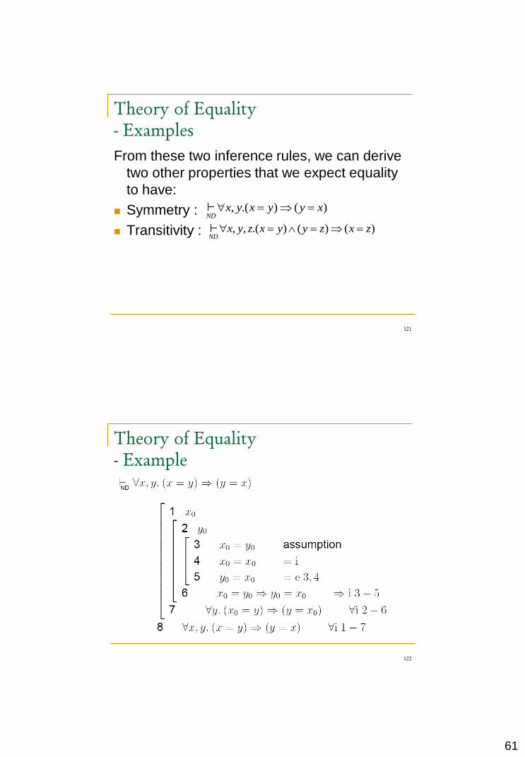
, .( ) ( )ND
x y x y y x
, , .( ) ( ) ( )ND
x y z x y y z x z
122
Theory of Equality
- Example

62
123
Theory of Equality
- Example
124
Theory of Equality
- Leibniz‟s Law
The substitution inference rule is related to
Leibniz‟s Law.
Leibniz‟s Law:
Leibniz‟s Law is generally referred to as the
ability to substitute “equals for equals”.
1 2 1 2if is a theorem, then so is [ / ] [ / ]t t P t x P t x
63
125
Leibniz
Gottfried Wilhelm von Leibniz (1646-1716)
The founder of differential and integral calculus.
Another of Leibniz‟s lifelong aims was to collate all human knowledge.
“[He was] one of the last great polymaths – not in the frivolous sense of having a wide general knowledge, but in the deeper sense of one who is a citizen of the whole world of intellectual inquiry.”
126
Theory of Equality
- Example
From our natural deduction rules, we can
derive Leibniz‟s Law:
1 2 1 2( ) ( )ND
t t P t P t

64
127
Theory of Equality
- Equality: Semantics
The semantics of the equality symbol is equality on the objects of the domain.
In ALL interpretations it means the same thing.
Normal interpretations are interpretations in which the symbol = is interpreted as designating the equality relation on the domain.
We will restrict ourselves to normal interpretations from now on.
128
Theory of Equality
- Extensional Equality
Equality in the domain is extensional, meaning it is
equality in meaning rather than form.
This is in contrast to intensional equality which is
equality in form rather than meaning.
In logic, we are interested in whether two terms
represent the same object, not whether they are the
same symbols.
If two terms are intensionally equal then they are
also extensionally equal, but not necessarily the
other way around.

65
129
Theory of Equality
- Equality: Counterexamples
Show the following argument is not valid:
where A,B are constants
. ( ) ( ), ( ), ( )x P x Q x P A A B Q B
130
Theory of Arithmetic
Another commonly used theory is that of
arithmetic.
It was formalized by Dedekind in 1879 and
also by Peano in 1889.
It is generally referred to as Peano‟s Axioms.
The model of the system is the natural
numbers with the constants 0 and 1, the
functions +, *, and the relation <.

66
131
Peano‟s Axioms
132
Intuitionistic Logic
“A proof that something exists is constructive if it provides a method for actually constructing it.”
In intuitionistic logic, only constructive proofs are allowed.
Therefore, they disallow proofs by contradiction. To show , you can‟t just show is impossible.
They also disallow the law of the excluded middle arguing that you have to actually show one of or before you can conclude
Intuitionistic logic was invented by Brouwer. Theorem provers that use intuitionistic logic are Nuprl, Coq, Elf, and Lego.
In this course, we will only be studying classical logic.
67
133
Summary
Predicate Logic (motivation, syntax and
terminology, semantics, axiom systems,
natural deduction)
Equality, Arithmetic
Mechanical theorem proving
Theorem proving
Formal Methods
Lecture 8
Farn Wang
Department of Electrical Engineering
National Taiwan University

68
Theorem Proving: Historical Perspective
Theorem proving (or automated deduction) =
logical deduction performed by machine
At the intersection of several areas
Mathematics: original motivation and techniques
Logic: the framework and the meta-reasoning
techniques
Theorem proving
Prove that an implementation satisfies a
specification by mathematical reasoning
implement Spec
implication
equivalence
or

69
Theorem proving
Implementation and specification expressed
as formulas in a formal logic
Required relationship (logical
equivalence/logical implication) described as
a theorem to be proven within the context of
a proof calculus
A proof system:
A set of axioms and inference rules (simplification,
rewriting, induction, etc.)
Proof checking
It is a purely syntactic matter to decide whether each theorem is an axiom or follows from previous theorems (axioms) by a rule of inference
Proof checker
“is this a proof?”Purported proof “Yes” / “No”

70
Proof generation
Complete automation generally impossible: theoretical undecidability limitations
However, a great deal can be automated (decidable subsets, specific classes of applications and specification styles)
Proof generator
“prove this theorem”purported theorem a proof
Applications
Hardware and software verification (or
debugging)
Automatic program synthesis from
specifications
Discovery of proofs of conjectures
A conjecture of Tarskiwas proved by machine
(1996)
There are effective geometry theorem provers

71
Program Verification
Fact: mechanical verification of software
would improve software productivity,
reliability, efficiency
Fact: such systems are still in experimental
stage
After 40 years !
Research has revealed formidable obstacles
Many believe that program verification is
extremely difficult
Program Verification
Fact:
Verification is done with respect to a specification
Is the specification simpler than the program ?
What if the specification is not right ?
Answer:
Developing specifications is hard
Still redundancy exposes many bugs as
inconsistencies
We are interested in partial specifications
An index is within bounds, a lock is released…

72
Programs, Theorems. Axiomatic Semantics
Consists of: A language for writing specifications about
programs
Rules for establishing when specifications hold
Typical specifications: During the execution, only non-null pointers are
dereferenced
This program terminates with x = 0
Partial vs. total correctness specifications Safety vs. liveness properties
Usually focus on safety (partial correctness)
Specification Languages
Must be easy to use and expressive (conflicting needs) Most often only expressive
Typically they are extensions of first-order logic Although higher-order or modal logics are also
used
We focus here on state-based specifications (safety) State = values of variables + contents of heap (+
past state) Not allowed: “variable x is live”, “lock L will be released”,
“there is no correlation between the values of x and y”

73
A Specification Language
We‟ll use a fragment of first-order logic: Formulas P ::= A | true | false | P1∧P2| P1∨P2| ¬P | ∀x.P
Atoms A ::= E1≤E2| E1= E2| f(A1,…,An) | …
※ All boolean expressions from our language are atoms
Can have an arbitrary collection of predicate symbols reachable(E1,E2) - list cell E2 is reachable from E1
sorted(a, L, H) - array a is sorted between L and H
ptr(E,T) - expression E denotes a pointer to T
E : ptr(T) - same in a different notation
An assertion can hold or not in a given state
Program Verification Using
Hoare’s Logic

74
Hoare Triples
Partial correctness: { P } s { Q } When you start s in any state that satisfies P
If the execution of s terminates
It does so in a state that satisfies Q
Total correctness: [ P ] s [ Q ] When you start sin any state that satisfies P
The execution of s terminates and
It does so in a state that satisfies Q
Defined inductively on the structure of statements
Hoare Rules
Assignments
y:=t
Composition
S1; S2
If-then-else
if e the S1 else S2
While
while e do S
Consequence

75
Greatest common divisor
{x1>0 x2>0}
y1:=x1;
y2:=x2;
while ¬ (y1=y2) do
if y1>y2 then y1:=y1-y2
else y2:=y2-y1
{y1=gcd(x1,x2)}
Why it works?
Suppose that y1,y2 are both positive integers.
If y1>y2 then gcd(y1,y2)=gcd(y1-y2,y2)
If y2>y1 then gcd(y1,y2)=gcd(y1,y2-y1)
If y1-y2 then gcd(y1,y2)=y1=y2

76
Hoare Rules: Assignment
General rule:
{p[t/y]} y:=t {p}
Examples:
{y+5=10} y:=y+5 {y=10}
{y+y<z} x:=y {x+y<z}
{2*(y+5)>20} y:=2*(y+5) {y>20}
Justification: write p with y’ instead of y, and
add the conjunct y’=t. Next, eliminate y’ by
replacing y’ by t.
Hoare Rules: Assignment
{p} y:=t {?}
Strategy: write p and the conjunct y=t, where y’ replaces
y in both p and t. Eliminate y’.
Example:
{y>5} y:=2*(y+5) {?}
{p} y:=t {y’ (p[y’/y] t[y’/y]=y)}
y’>5 y=2*(y’+5) y>20

77
Hoare Rules: Composition
General rule:
{p} S1 {r}, {r} S2 {q} {p} S1;S2 {q}
Example:
if the antecedents are
1. {x+1=y+2} x:=x+1 {x=y+2}
2. {x=y+2} y:=y+2 {x=y}
Then the consequent is
{x+1=y+2} x:=x+1; y:=y+2 {x=y}
Hoare Rules: If-then-else
General rule:
{p e} S1 {q}, {p ¬ e} S2 {q}
{p} if e then S1 else S2 {q}
Example:
p is gcd(y1,y2)=gcd(x1,x2) y1>0 y2>0
¬ (y1=y2)
e is y1>y2
S1 is y1:=y1-y2
S2 is y2:=y2-y1
q is gcd(y1,y2)=gcd(x1,x2) y1>0 y2>0

78
Hoare Rules: While
General rule:
{p e} S {p}
{p} while e do S {p ¬ e}
Example:
p is {gcd(y1,y2)=gcd(x1,x2) y1>0 y2>0}
e is (y1 y2)
S is if y1>y2 then y1:=y1-y2 else y2:= y2-y1
Hoare Rules: Consequence
Strengthen a precondition
rp, {p} S {q}
{r} S {q}
Weaken a postcondition
{p} S {q}, qr
{p} S {r}

79
Soundness
Hoare logic is sound in the sense that
everything that can be proved is correct!
This follows from the fact that each axiom
and proof rule preserves soundness.
Completeness
A proof system is called complete if every
correct assertion can be proved.
Propositional logic is complete.
No deductive system for the standard
arithmetic can be complete (Godel).

80
And for Hoare logic?
Let S be a program and p its precondition.
Then {p} S {false} means that S never
terminates when started from p. This is
undecidable. Thus, Hoare’s logic cannot be
complete.
Hoare Rules: Examples
Consider
{ x = 2 } x := x + 1 { x < 5 }
{ x < 2 } x := x + 1 { x < 5 }
{ x < 4 } x := x + 1 { x < 5 }
They all have correct preconditions
But the last one is the most general (or
weakest) precondition

81
Dijkstra’s Weakest Preconditions
Consider { P } s { Q }
Predicates form a lattice:
valid precondictions
false true
strong weak
To verify { P } s { Q }
compute WP(s, Q) and prove P WP(s, Q)
Weakest prendition,
Strongest postcondition
For an assertion p and code S, let post(p,S)
be the strongest assertion such that
{p}S{post(p,S)}
That is, if {p}S{q} then post(p,S)q.
For an assertion q and code S, let pre(S,q)
be the weakest assertion such that
{pre(S,q)}S{q}
That is, if {p}S{q} then ppre(S,q).

82
Relative completeness
Suppose that either
post(p,S) exists for each p, S, or
pre(S,q) exists for each S, q.
Some oracle decides on pure implications.
Then each correct Hoare triple can be proved.
What does that mean? The weakness of the
proof system stem from the weakness of the
(FO)
logic, not of Hoare’s proof system.
Extensions
Many extensions for Hoare’s proof rules:
Total correctness
Arrays
Subroutines
Concurrent programs
Fairness

83
Higher-Order Logic
Higher-Order Logic
First-order logic:
only domain variables can be quantified.
Second-order logic:
quantification over subsets of variables (i.e., over
predicates).
Higher-order logics:
quantification over arbitrary predicates and
functions.

84
Higher-Order Logic
Variables can be functions and predicates,
Functions and predicates can take functions as arguments and return functions as values,
Quantification over functions and predicates.
Since arguments and results of predicates and functions can themselves be predicates or functions, this imparts a first-class status to functions, and allows them to be manipulated just like ordinary values
Higher-Order Logic
Example 1: (mathematical induction)
P. [P(0) (n. P(n)P(n+1))] n.P(n)
(Impossible to express it in FOL)
Example 2:
Function Rise defined as Rise(c, t) = c(t) c(t+1)
Rise expresses the notion that a signal c rises at time t.
Signal is modeled by a function c: N {F,T}, passed as
argument to Rise.
Result of applying Rise to c is a function: N {F,T}.

85
Higher-Order Logic (cont’d)
Advantage:
high expressive power!
Disadvantages:
Incompleteness of a sound proof system for most
higher-order logics
Theorem (Gödel, 1931)
There is no complete deduction system for the
second-order logic.
Reasoning more difficult than in FOL, need
ingenious inference rules and heuristics.
Higher-Order Logic (cont’d)
Disadvantages: Inconsistencies can arise in higher-order systems if semantics
not carefully defined
“Russell Paradox”:
Let P be defined by P(Q) = Q(Q). By substituting P for Q, leads to P(P) = P(P),
(P: bool bool, Q: bool bool)
Introduction of “types” (syntactical mechanism) is effective against certain inconsistencies.
Use controlled form of logic and inferences to minimize the risk of inconsistencies, while gaining the benefits of powerful representation mechanism.
Higher-order logic increasingly popular for hardware verification!
Contradiction!

86
Theorem Proving Systems
Automated deduction systems (e.g. Prolog) full automatic, but only for a decidable subset of
FOL
speed emphasized over versatility
often implemented by ad hoc decision procedures
often developed in the context of AI research
Interactive theorem proving systems semi-automatic, but not restricted to a decidable
subset
versatility emphasized over speed
in principle, a complete proof can be generated for every theorem
Theorem Proving Systems
Some theorem proving systems:
Boyer-Moore (first-order logic)
HOL (higher-order logic)
PVS (higher-order logic)
Lambda (higher-order logic)

87
HOL
HOL (Higher-Order Logic) developed at University of Cambridge
Interactive environment (in ML, Meta Language) for machine assisted theorem proving in higher-order logic (a proof assistant)
Steps of a proof are implemented by applying inference rules chosen by the user; HOL checks that the steps are safe
All inferences rules are built on top of eight primitive inference rules
HOL
Mechanism to carry out backward proofs by
applying built-in ML functions called tactics
and tacticals
By building complex tactics, the user can
customize proof strategies
Numerous applications in software and
hardware verification
Large user community

88
HOL Theorem Prover
Logic is strongly typed (type inference, abstract data
types, polymorphic types, etc.)
It is sufficient for expressing most ordinary mathematical
theories (the power of this logic is similar to set theory)
HOL provides considerable built-in theorem-proving
infrastructure:
a powerful rewriting subsystems
library facility containing useful theories and tools for general use
Decision procedures for tautologies and semi-decision procedure
for linear arithmetic provided as libraries
HOL Theorem Prover
The primary interface to HOL is the functional programming language ML
Theorem proving tools are functions in ML (users of HOL build their own application specific theorem proving infrastructure by writing programs in ML)
Many versions of HOL: HOL88: Classic ML (from LCF);
HOL90: Standard ML
HOL98: Moscow ML

89
HOL Theorem Prover (cont’d)
The HOL systems can be used in two main ways:
for directly proving theorems: when higher-order logic is a suitable specification language (e.g., for hardware verification and classical mathematics)
as embedded theorem proving support for application-specific verification systems when specification in specific formalisms needed to be supported using customized tools.
The approach to mechanizing formal proof used in HOL is due to Robin Milner.
He designed a system, called LCF: Logic for Computable Functions. (The HOL system is a direct descendant of LCF.)
HOL and ML
The ML Language
Some predefined functions + typesHOL =
Specification in HOL
Functional description:express output signal as function of input signals, e.g.:
AND gate:
out = and (in1, in2) = (in1 in2)
Relational (predicate) description:
gives relationship between inputs and outputs in the form of a
predicate (a Boolean function returning “true” of “false”), e.g.:
AND gate:
AND ((in1, in2),(out)):= out =(in1 in2)
in1in2
out

90
Specification in HOL
Notes:
functional descriptions allow recursive functions to
be described. They cannot describe bi-directional
signal behavior or functions with multiple feed-
back signals, though
relational descriptions make no difference
between inputs and outputs
Specification in HOL will be a combination of
predicates, functions and abstract types
Specification in HOL
conjunction “” of implementation module predicates
M (a, b, c, d, e):= M1 (a, b, p, q) M2 (q, b, e) M3 (e, p, c, d)
hide internal lines (p,q) using existential quantification
M (a, b, c, d, e):= p q. M1 (a, b, p, q) M2 (q, b, e) M3 (e, p, c, d)
Network of modules
M1
M2
M3ab
cd
e
p
q
M

91
Specification in HOL
SPEC (in1, in2, in3, in4, out):=
out = (in1 in2) (in3 in4)
IMPL (in1, in2, in3, in4, out):=
l1, l2. AND (in1, in2, l1) AND (in3, in4, l2) OR (l1, l2, out)
where AND (a, b, c):= (c =a b)
OR (a, b, c):= (c = a b)
Combinational circuits
in1in2
in3in4
I1
I2
out
Specification in HOL
Note: a functional description would be:
IMPL (in1, in2, in3, in4, out):=
out = (or (and (in1, in2), and (in3, in4))
where and (in1, in2) = (in1 in2)
or (in1, in2) = (in1 in2)
92
Specification in HOL
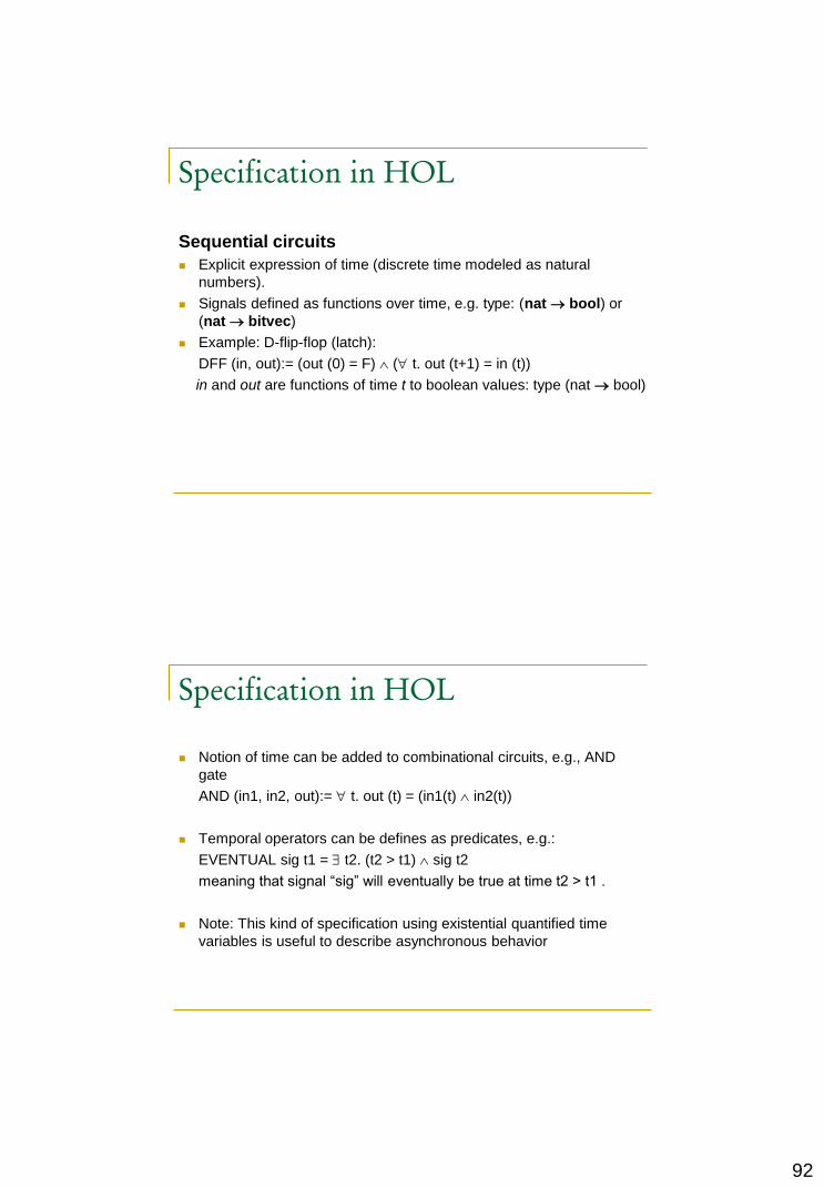
Sequential circuits
Explicit expression of time (discrete time modeled as natural
numbers).
Signals defined as functions over time, e.g. type: (nat bool) or
(nat bitvec)
Example: D-flip-flop (latch):
DFF (in, out):= (out (0) = F) ( t. out (t+1) = in (t))
in and out are functions of time t to boolean values: type (nat bool)
Specification in HOL
Notion of time can be added to combinational circuits, e.g., AND
gate
AND (in1, in2, out):= t. out (t) = (in1(t) in2(t))
Temporal operators can be defines as predicates, e.g.:
EVENTUAL sig t1 = t2. (t2 > t1) sig t2
meaning that signal “sig” will eventually be true at time t2 > t1 .
Note: This kind of specification using existential quantified time
variables is useful to describe asynchronous behavior

93
HOL Proof Mechanism
A formal proof is a sequence, each of whose
elements is
either an axiom
or follows from earlier members of the sequence
by a rule of inference
A theorem is the last element of a proof
A sequent is written:
P, where is a set of assumptions and P is
the conclusion
HOL Proof Mechanism
In HOL, this consists in applying ML functions representing rules of inference to axioms or previously generated theorems
The sequence of such applications directly correspond to a proof
A value of type thm can be obtained either directly (as an axiom)
by computation (using the built-in functions that represent the inference rules)
ML typechecking ensures these are the only ways to generate a thm:
All theorems must be proved!

94
Verification Methodology in HOL
1. Establish a formal specification (predicate) of the
intended behavior (SPEC)
2. Establish a formal description (predicate) of the
implementation (IMP), including:
behavioral specification of all sub-modules
structural description of the network of sub-modules
3. Formulation of a proof goal, either
IMP SPEC (proof of implication), or
IMP SPEC (proof of equivalence)
4. Formal verification of above goal using a set of
inference rules
Example 1: Logic AND
AND Specification:
AND_SPEC (i1,i2,out) := out = i1 i2
NAND specification:
NAND (i1,i2,out) := out = (i1 i2)
NOT specification:
NOT (i, out) := out = I
AND Implementation:
AND_IMPL (i1,i2,out) := x. NAND (i1,i2,x) NOT (x,out)
xi1i2
out
AND
i1i2
out
i out

95
Example 1: Logic AND
Proof Goal: i1, i2, out. AND_IMPL(i1,i2,out) ANDSPEC(i1,i2,out)
Proof (forward)
AND_IMP(i1,i2,out) {from above circuit diagram}
x. NAND (i1,i2,x) NOT (x,out) {by def. of AND impl}
NAND (i1,i2,x) NOT(x,out) {strip off “ x.”}
NAND (i1,i2,x) {left conjunct of line 3}
x = (i1 i2) {by def. of NAND}
NOT (x,out) {right conjunct of line 3}
out = x {by def. of NOT}
out = ((i1 i2) {substitution, line 5 into 7}
out =(i1 i2) {simplify, t=t}
AND (i1,i2,out) {by def. of AND spec}
AND_IMPL (i1,i2,out) AND_SPEC (i1,i2,out)
Q.E.D.
Example 2: CMOS-Inverter
Specification (black-box behavior)
Spec(x,y):= (y = ¬ x)
Implementation
Basic Modules Specs
PWR(x):= (x = T)
GND(x):= (x = F)
N-Trans(g,x,y):= (g (x = y))
P-Trans(g,x,y):= (¬ g (x = y))
p
q
x y
(P-Trans)
(N-Trans)

96
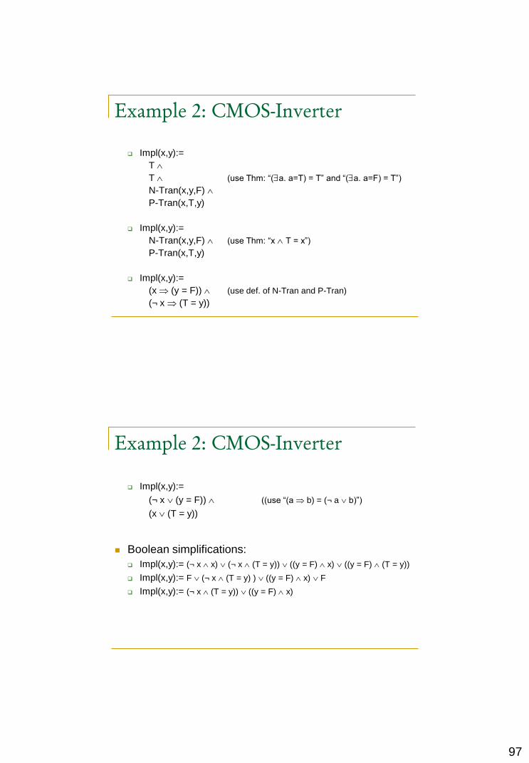
Example 2: CMOS-Inverter
Implementation (network structure) Impl(x,y):= p, q.
PWR(p)
GND(q)
N-Tran(x,y,q)
P-Tran(x,p,y)
Proof goal x, y. Impl(x,y) Spec(x,y)
Proof (forward) Impl(x,y):= p, q.
(p = T)
(q = F) (substitution of the definition of PWR and GND)
N-Tran(x,y,q)
P-Tran(x,p,y)
Example 2: CMOS-Inverter
Impl(x,y):= p q.
(p = T)
(q = F) (substitution of p and q in P-Tran and N-Tran)
N-Tran(x,y,F)
P-Tran(x,T,y)
Impl(x,y):=
( p. p = T)
( q. q = F) (use Thm: “a. t1 t2 = (a. t1) t2” if a is free in t2)
N-Tran(x,y,F)
P-Tran(x,T,y)
97
Example 2: CMOS-Inverter
Impl(x,y):=
T
T (use Thm: “(a. a=T) = T” and “(a. a=F) = T”)
N-Tran(x,y,F)
P-Tran(x,T,y)
Impl(x,y):=
N-Tran(x,y,F) (use Thm: “x T = x”)
P-Tran(x,T,y)
Impl(x,y):=
(x (y = F)) (use def. of N-Tran and P-Tran)
(¬ x (T = y))
Example 2: CMOS-Inverter
Impl(x,y):=
(¬ x (y = F)) ((use “(a b) = (¬ a b)”)
(x (T = y))
Boolean simplifications:
Impl(x,y):= (¬ x x) (¬ x (T = y)) ((y = F) x) ((y = F) (T = y))
Impl(x,y):= F (¬ x (T = y) ) ((y = F) x) F
Impl(x,y):= (¬ x (T = y)) ((y = F) x)

98
Example 2: CMOS-Inverter
Case analysis x=T/F x=T:Impl(T,y):= (F (T = y) ) ((y = F) T)
x=F:Impl(F,y):= (T (T = y) ) ((y = F) F)
x=T:Impl(T,y):= (y = F)
x=F:Impl(F,y):= (T = y)
Case analysis on Spec: x=T:Spec(T,y):= (y = F)
x=F:Spec(F,y):= (y = T)
Conclusion: Spec(x,y) Impl(x,y)
=
Abstraction Forms
Structural abstraction:
only the behavior of the external inputs and outputs of a module
is of interest (abstracts away any internal details)
Behavioral abstraction:
only a specific part of the total behavior (or behavior under
specific environment) is of interest
Data abstraction:
behavior described using abstract data types (e.g. natural
numbers instead of Boolean vectors)
Temporal abstraction:
behavior described using different time granularities (e.g.
refinement of instruction cycles to clock cycles)

99
Example 3: 1-bit Adder
Specification:
ADDER_SPEC (in1:nat, in2:nat, cin:nat, sum:nat, cout:nat):=
in1+in2 + cin = 2*cout + sum
Implementation:
Note: Spec is a structural abstraction of Impl.
1-bit
ADDER
sum
cout
in1in2cin
sum
cout
in1in2
cin
I1
I2
I3
1-bit Adder (cont’d)
Implementation:
ADDER_IMPL(in1:bool, in2:bool, cin:bool, sum:bool, cout:bool):=
l1 l2 l3. EXOR (in1, in2, l1)
AND (in1, in2, l2)
EXOR (l1,cin,sum)
AND (l1, cin, l3)
OR (l2, l3, cout)
Define a data abstraction function (bn: bool nat) needed to relate
Spec variable types (nat) to Impl variable types (bool):
bn(x) :=
1, if x = T
0, if x = F

100
1-bit Adder (cont’d)
Proof goal:
in1, in2, cin, sum, cout.
ADDER_IMPL (in1, in2, cin, sum, cout)
ADDER_SPEC (bn(in1), bn(in2), bn(cin), bn(sum), bn(cout))
Verification of Generic Circuits
used in datapath design and verification
idea:
verify n-bit circuit then specialize proof for specific
value of n, (i.e., once proven for n, a simple
instantiation of the theorem for any concrete value,
e.g. 32, gets a proven theorem for that instance).
use of induction proof

101
Example 4: N-bit Adder
N-bit Adder
Specification
N-ADDER_SPEC (n,in1,in2,cin,sum,cout):=
(in1 + in2 + cin = 2n+1 * cout + sum)
n-bit
ADDER
sum[0..1]
cout
in1[0..n-1]in2[0..n-1]
cin
Example 4: N-bit Adder
Implementation
1-bit
ADDER sum[n-1]
coutin1[n-1]in2[n-1]
cin
1-bit
ADDER
1-bit
ADDER
in1[n-2]in2[n-2]
in1[0]in2[0]
sum[n-2]
sum[0]
……
w
102
N-bit Adder (cont’d)
Implementation
recursive definition:
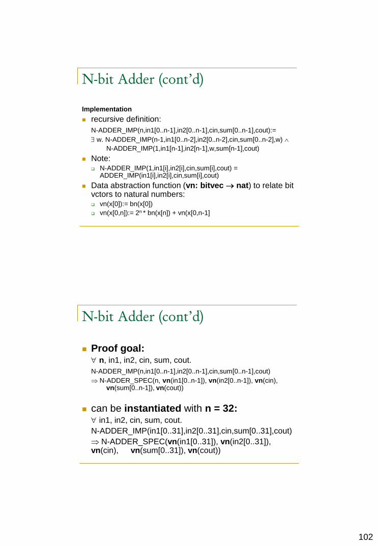
N-ADDER_IMP(n,in1[0..n-1],in2[0..n-1],cin,sum[0..n-1],cout):=
w. N-ADDER_IMP(n-1,in1[0..n-2],in2[0..n-2],cin,sum[0..n-2],w)
N-ADDER_IMP(1,in1[n-1],in2[n-1],w,sum[n-1],cout)
Note: N-ADDER_IMP(1,in1[i],in2[i],cin,sum[i],cout) =
ADDER_IMP(in1[i],in2[i],cin,sum[i],cout)
Data abstraction function (vn: bitvec nat) to relate bit vctors to natural numbers: vn(x[0]):= bn(x[0])
vn(x[0,n]):= 2n * bn(x[n]) + vn(x[0,n-1]
N-bit Adder (cont’d)
Proof goal: n, in1, in2, cin, sum, cout.
N-ADDER_IMP(n,in1[0..n-1],in2[0..n-1],cin,sum[0..n-1],cout)
N-ADDER_SPEC(n, vn(in1[0..n-1]), vn(in2[0..n-1]), vn(cin), vn(sum[0..n-1]), vn(cout))
can be instantiated with n = 32: in1, in2, cin, sum, cout.
N-ADDER_IMP(in1[0..31],in2[0..31],cin,sum[0..31],cout)
N-ADDER_SPEC(vn(in1[0..31]), vn(in2[0..31]), vn(cin), vn(sum[0..31]), vn(cout))

103
N-bit Adder (cont’d)
Proof by induction over n:
basis step:N-ADDER_IMP(0,in1[0],in2[0],cin,sum[0],cout)
N-ADDER_SPEC(0,vn(in1[0]),vn(in2[0]),vn(cin),vn(sum[0]),vn(cout))
induction step:[N-ADDER_IMP(n,in1[0..n-1],in2[0..n-1],cin,sum[0..n-1],cout)
N-ADDER_SPEC(n,vn(in1[0..n-1]),vn(in2[0..n-1]),vn(cin),vn(sum[0..n-1]),vn(cout))]
[N-ADDER_IMP(n+1,in1[0..n],in2[0..n],cin,sum[0..n],cout)
N-ADDER_SPEC(n+1,vn(in1[0..n]),vn(in2[0..n]),vn(cin),vn(sum[0..n]),vn(cout))]
N-bit Adder (cont’d)
Notes:
basis step is equivalent to 1-bit adder proof, i.e.ADDER_IMP(in1[0],in2[0],cin,sum[0],cout)
ADDER_SPEC(bn(in1[0]),bn(in2[0]),bn(cin),bn(sum[0]),bn(cout))
induction step needs more creativity and work load!

104
Practical Issues of Theorem Proving
No fully automatic theorem provers. All require
human guidance in indirect form, such as:
When to delete redundant hypotheses, when to keep a
copy of a hypothesis
Why and how (order) to use lemmas, what lemma to use
is an art
How and when to apply rules and rewrites
Induction hints (also nested induction)
Practical Issues of Theorem Proving
Selection of proof strategy, orientation of equations, etc.
Manipulation of quantifiers (forall, exists)
Instantiation of specification to a certain time and
instantiating time to an expression
Proving lemmas about (modulus) arithmetic
Trying to prove a false lemma may be long before
abandoning

105
PVS
Prototype Verification System (PVS)
Provides an integrated environment for the
development and analysis of formal
specifications.
Supports a wide range of activities involved in
creating, analyzing, modifying, managing,
and documenting theories and proofs.

106
Prototype Verification System
(cont’)
The primary purpose of PVS is to provide
formal support for conceptualization and
debugging in the early stages of the lifecycle
of the design of a hardware or software
system.
In these stages, both the requirements and
designs are expressed in abstract terms that
are not necessarily executable.
Prototype Verification System
(cont’)
The primary emphasis in the PVS proof
checker is on supporting the construction of
readable proofs.
In order to make proofs easier to develop, the
PVS proof checker provides a collection of
powerful proof commands to carry out
propositional, equality, and arithmetic
reasoning with the use of definitions and
lemmas.

107
The PVS Language
The specification language of PVS is built on higher-order logic Functions can take functions as arguments and
return them as values
Quantification can be applied to function variables
There is a rich set of built-in types and type-constructors, as well as a powerful notion of subtype.
Specifications can be constructed using definitions or axioms, or a mixture of the two.
The PVS Language (cont’)
Specifications are logically organized into
parameterized theories and datatypes.
Theories are linked by import and export lists.
Specifications for many foundational and
standard theories are preloaded into PVS as
prelude theories that are always available
and do not need to be explicitly imported.

108
A Brief Tour of PVS
Creating the specification
Parsing
Typechecking
Proving
Status
Generating LATEX
A Simple Specification Example
sum: Theory
BEGIN
n: VAR nat
sum(n): RECURSIVE nat =
(IF n = 0 THEN 0 ELSE n + sum(n-1) ENDIF)
MEASURE (LAMBDA n : n)
closed_form: THEOREM sum(n) = (n * (n + 1)) / 2
END sum

109
Creating the Specification
Create a file with a .pvs extension
Using the M-x new-pvs-file command (M-x nf) to create a new
PVS file, and typing sum when prompted. Then type in the sum
specification.
Since the file is included on the distribution tape in the
Examples/tutorial subdirectory of the main PVS directory, it can
be imported with the M-x import-pvs-file command (M-x imf). Use
the M-x whereis-pvs command to find the path of the main PVS
directory.
Finally, any external means of introducing a file with
extension .pvs into the current directory will make it available to
the system. ex: using vi.
Parsing
Once the sum specification is displayed, it
can be parsed with the M-x parse (M-x pa)
command, which creates the internal abstract
representation for the theory described by the
specification.
If the system finds an error during parsing, an
error window will pop up with an error
message, and the cursor will be placed in the
vicinity of the error.

110
Typechecking
To typecheck the file by typing M-x typecheck
(M-x tc, C-c t), which checks for semantic
errors, such as undeclared names and
ambiguous types.
Typechecking may build new files or internal
structures such as TCCs. (when sum has
been typechecked, a message is displayed in
the minibuffer indicating the two TCCs were
generated)
Typechecking (cont’)
These TCCs represent proof obligations that
must be discharged before the sum theory
can be considered typechecked.
TCCs can be viewed using the M-x show-tccs
command.

111
Typechecking (cont’)
% Subtype TCC generated (line 7) for n-1
% unchecked
sum_TCC1: OBLIGATION (FORALL (n : nat) : NOT n=0 IMPLIES n-1 >= 0);
% Termination TCC generated (line 7) for sum
% unchecked
sum_TCC2: OBLIGATION (FORALL (n : nat) : NOT n=0 IMPLIES n-1 < n);
Typechecking (cont’)
The first TCC is due to the fact that sum takes an argument of
type nat, but the type of the argument in the recursive call to sum
is integer, since nat is not closed under substraction.
Note that the TCC includes the condition NOT n=0, which holds
in the branch of the IF-THEN-ELSE in which the expression n-1
occirs.
The second TCC is needed to ensure that the function sum is
total. PVS does not directly support partial functions, although its
powerful subtyping mechanism allows PVS to express many
operations that are traditionally regarded as partial.
The measure function is used to show that recursive definitions
are total by requiring the measure to decrease with each
recursive call.

112
Proving
We are now ready to try to prove the main
theorem
Place the cursor on the line containing the
closed form theorem and type M-x prove M-x
pr or C-c p
A new buer will pop up the formula will be
displayed and the cursor will appear at the
Rule prompt indicating that the user can
interact with the prover
Proving (cont’)
First, notice the display, which consists of a single
formula labeled {1} under a dashed line.
This is a sequent: formulas above the dashed lines are
called antecedents and those below are called
succedents
The interpretation of a sequent is that the conjunction of the
antecedents implies the disjunction of the succedents
Either or both of the antecedents and succedents may be empty

113
Proving (cont’)
The basic objective of the proof is to generate a proof tree in which all of the leaves are trivially true
The nodes of the proof tree are sequents and while in the prover you will always be looking at an unproved leaf of the tree
The current branch of a proof is the branch leading back to the root from the current sequent
When a given branch is complete (i.e., ends in a true leaf), the prover automatically moves on to the next unproved branch, or, if there are no more unproven branches, notifies you that the proof is complete
Proving (cont’)
We will prove this formula by induction n.
To do this, type (induct “n”)
This generates two subgoals the one displayed is
the base case where n is 0
To see the inductive step type (postpone) which
postpones the current subgoal and moves on to
the next unproved one Type (postpone) a second
time to cycle back to the original subgoal (labeled
closed_form.1)

114
Proving (cont’)
To prove the base case, we need to expand the denition of sum, which is done by typing (expand “sum”)
After expanding the denition of sum, we send the proof to the PVS decision procedures, which automatically decide certain fragments of arithmetic, by typing (assert)
This completes the proof of this subgoal and the system moves on to the next subgoal which is the inductive step
Proving (cont’)
The first thing to do here is to eliminate the FORALL
quantifier
This can most easily be done with the skolem! command,
which provides new constants for the bound variables
To invoke this command type (skolem!) at the prompt
The resulting formula may be simplified by typing (flatten),
which will break up the succedent into a new antecedent
and succedent
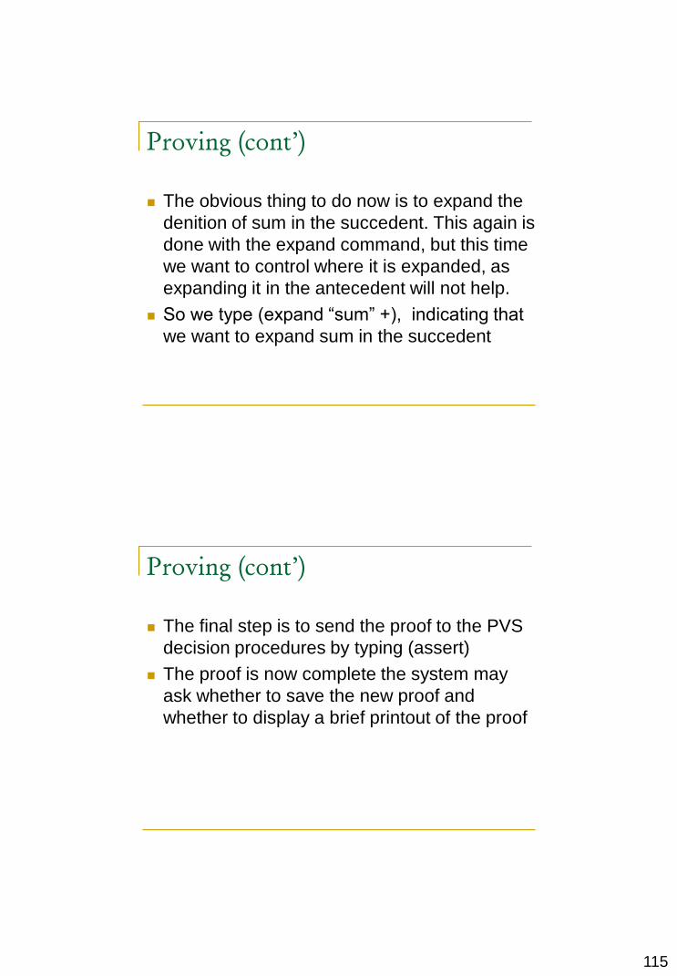
115
Proving (cont’)
The obvious thing to do now is to expand the
denition of sum in the succedent. This again is
done with the expand command, but this time
we want to control where it is expanded, as
expanding it in the antecedent will not help.
So we type (expand “sum” +), indicating that
we want to expand sum in the succedent
Proving (cont’)
The final step is to send the proof to the PVS
decision procedures by typing (assert)
The proof is now complete the system may
ask whether to save the new proof and
whether to display a brief printout of the proof

116
closed_form :
| - - - - - - -
{1} (FORALL (n : nat) : sum(n) = (n * (n + 1)) / 2)
Rule? (induct “n”)
Inducting on n,
this yields 2 subgoals
closed_form.1 :
| - - - - - - -
{1} sum(0) = (0 * (0 + 1)) / 2
Rule? (postpone)
Postponing closed_form.1
closed_form.2 :
| - - - - - - -
{1} (FORALL (j : nat) :
sum(j) = (j * (j + 1)) / 2
IMPLIES sum(j + 1) = ((j + 1) * (j + 1 + 1)) / 2
Rule? (postpone)
Postponing closed_form.2
closed_form.1 :
| - - - - - - -
{1} sum(0) = (0 * (0 + 1)) / 2
Rule? (expand “sum”)
(IF 0 = 0 THEN 0 ELSE 0 + sum(0 - 1) ENDIF)

117
simplifies to 0
Expanding the definition of sum,
this simplifies to:
closed_form.1 :
| - - - - - - -
{1} 0 = 0 / 2
Rule? (assert)
Simplifying, rewriting, and recording with decision procedures,
This completes the proof of closed_form.1.
closed_form.2 :
| - - - - - - -
{1} (FORALL (j : nat) :
sum(j) = (j * (j + 1)) / 2
IMPLIES sum(j + 1) = ((j + 1) * (j + 1 + 1)) / 2
Rule? (skolem!)
Skolemizing,
this simplifies to:
closed_form.2 | - - - - - - -
{1} sum(j ! 1) = (j ! 1 * (j ! 1 + 1)) / 2
IMPLIES sum(j ! 1 + 1) = ((j ! 1 + 1) * (j ! 1 + 1 + 1)) / 2
Rule? (flatten)
Applying disjunctive simplification to flatten sequent,
This simplifies to:
closed_form.2 :
{-1}sum(j ! 1) = (j ! 1 * (j ! 1 + 1)) / 2
| - - - - - - -
{1} sum(j ! 1 + 1) = ((j ! 1 + 1) * (j ! 1 + 1 + 1)) / 2

118
Rule? (expand “sum” +)
(IF j ! 1 + 1 = 0 THEN 0 ELSE j ! 1 + 1 + sum(j ! 1 + 1 - 1) ENDIF)
simplifies to 1 + sum(j ! 1) + j ! 1
Expanding the definition of sum,
this simplifies to:
closed_form.2:
[-1] sum(j ! 1) = (j ! 1 * (j ! 1 + 1)) / 2
| - - - - - - -
{1} 1 + sum(j ! 1) + j ! 1 = (2 + j ! 1 + (j ! 1 * j ! 1 + 2 * j ! 1)) / 2
Rule? (assert)
Simplifying, rewriting, and recording with decision procedures,
This completes the proof of closed_form.2.
Q.E.D
Run time = 5.62 secs.
Real time= 58.95 secs.
Status
Type M-x status-proof-theory (M-x spt) and
you will see a buffer which displays the
formulas in sum (including the TCCs), along
with an indication of their proof status
This command is useful to see which formulas
and TCCs still require proofs
Another useful command is M-x status-
proofchain (M-x spc), which analyzes a given
proof to determine its dependencies
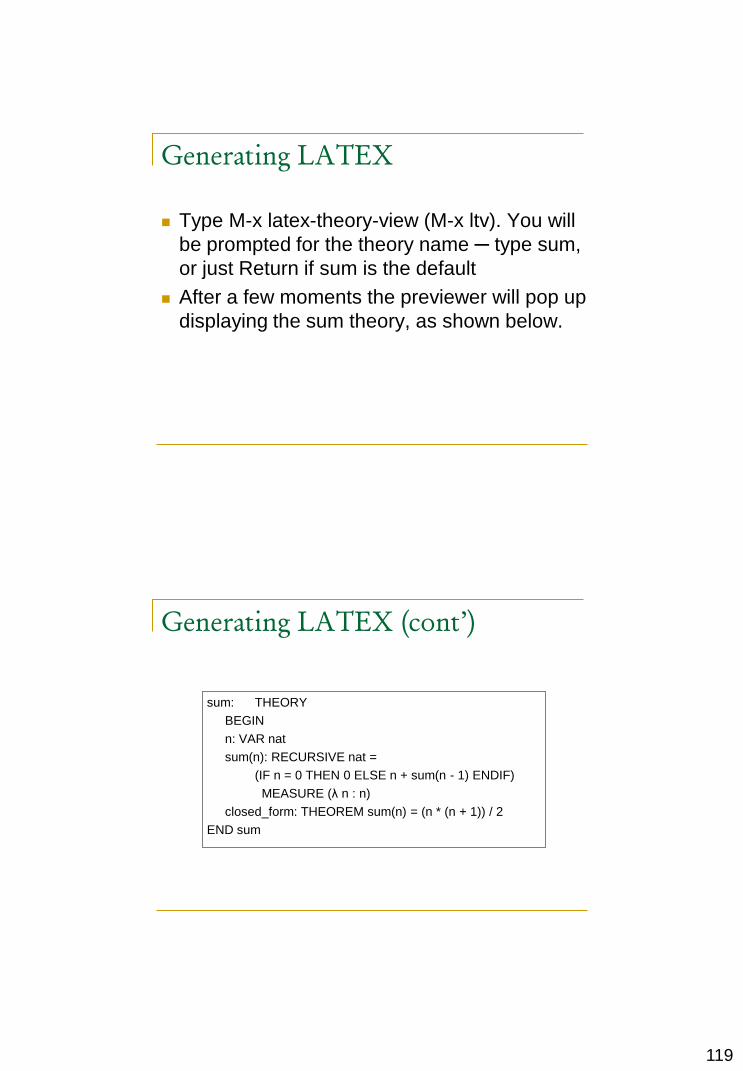
119
Generating LATEX
Type M-x latex-theory-view (M-x ltv). You will
be prompted for the theory name ─ type sum,
or just Return if sum is the default
After a few moments the previewer will pop up
displaying the sum theory, as shown below.
Generating LATEX (cont’)
sum: THEORY
BEGIN
n: VAR nat
sum(n): RECURSIVE nat =
(IF n = 0 THEN 0 ELSE n + sum(n - 1) ENDIF)
MEASURE (λ n : n)
closed_form: THEOREM sum(n) = (n * (n + 1)) / 2
END sum

120
Generating LATEX (cont’)
Finally using the M-x latex-proof command, it
is possible to generate a LATEX file from a
proof
Expanding the definition of sum
closeed_form.2:
'
0{ 1} ( ' ( ' 1)) / 2
j
ii j j
' 1 1
0{1} (IF ' 1 0 THEN 0 ELSE ' 1 ENDIF) (( ' 1) ( ' 1 1)) / 2
j
ij j i j j
Conclusions
Advantages of Theorem Proving
High abstraction and expressive notation
Powerful logic and reasoning, e.g., induction
Can exploit hierarchy and regularity, puts user in control
Can be customized with tactics (programs that build
larger proofs steps from basic ones)
Useful for specifying and verifying parameterized
(generic) datapath-dominated designs
Unrestricted applications (at least theoretically)

121
Conclusions
Limitations of Theorem Proving: Interactive (under user guidance): use many lemmas,
large numbers of commands
Large human investment to prove small theorems
Usable only by experts: difficult to prove large / hard theorems
Requires deep understanding of the both the design and HOL (while-box verification)
must develop proficiency in proving by working on simple but similar problems.
Automated for narrow classes of designs