Lecture Guide

CBMS Conference on Applications of Polynomial Systems

Texas Christian University, June 4-8, 2018

David A. Cox, Principal Lecturer

Introduction

This guide is designed as a supplement to my lectures at the conference. It serves threemain purposes:

• Suggest background readings for the topics covered in the lectures.• Summarize briefly the content of each lecture.• Provide complete references for all papers and books mentioned in the lectures.

About a year ago, I wrote a tentative description of the lectures, available at the conferencewebsite under the heading Abstracts of Professor Cox’s talks. However, in the process ofwriting the lectures, I found them taking on a life of their own that often diverged from myoriginal conception. This guide is based on the actual lectures.

Each day of the conference is devoted to a different topic:

Monday: Elimination TheoryTuesday: Numerical Algebraic GeometryWednesday: Geometric ModelingThursday: Rigidity TheoryFriday: Chemical Reaction Neworks

There will be three lectures per day: two given by me, and the third given by an expert inthe field. I am extremely grateful to Carlos D’Andrea, Jon Hauenstein, Hal Schenck, JessicaSidman, and Alicia Dickenstein for agreeing to be part of the conference. You will enjoytheir lectures.

The references at the end of this document fall into two groups:

• Background references, which you might want to look at before the conference begins.These are numbered [B1], [B2], etc.

• References for all papers mentioned in my lectures. These are numbered [1], [2], etc.

Besides the five topics listed above, the twin themes toric varieties and algebraic statistics

play a prominent role in the lectures. The papers [B2] and [B7] give the background needed.

Monday: Elimination Theory

Elimination theory has important roles to play in both algebraic geometry and symboliccomputation. I will take a historical approach in my lectures on this subject so that you cansee how elimination theory has developed over the years.

Background Reading: [B3, Chapters 2, 3], [B4, Chapters 3, 7], [B9, Sections 1–3].

§1: Elimination Theory in the 18th and 19th Centuries. In spite of the title, I will begin inthe 17th century with examples from Newton (1666) [93] and Tschirnhaus (1683) [114] toillustrate the geometric and algebraic aspects of elimination. In the 18th century, what wecall Bezout’s theorem for the plane was well known (e.g., Cramer (1750) [39]) and people,including Bezout (1764) [17], were already thinking about other versions of the theorem.

1

I will spend some time on Waring’s Meditationes Algebraicæ (1772) [122] and Bezout’s

Theorie Generale des Equations Algebriques (1779) [18]. The latter is 500 pages long and in-cludes many versions of the theorem. In modern terms, Bezout’s formulas are the normalizedvolumes of certain Newton polytopes. You will see some astonishing pictures. Penchevre’sarticle [B9] describes what Bezout did in more detail.

Another important tool was the Poisson formula for the resultant, published in 1802 byPoisson [95]. But it wasn’t until later in the 19th century that the subject exploded withpapers and books by Sylvester (1840) [111], Cayley (1864) [30], Brill (1880) [22], Kronecker(1882) [80], Mertens (1886) [87], Netto (1900) [91], Macaulay (1903, 1916) [84, 85], and manyothers. The 1907 review article of Netto and Le Vavasseur [92, pp. 73–169] (97 pages long)and 2006 PhD thesis of Penchevre (317 pages long) survey the substantial body of the workled to the theory of what we now call the dense or classical resultant. At the same time,people explored various aspects of resultants, which I will illustrate using examples frompapers by Minding (1841) [90], Bonnet (1847) [21], and Riemann (1857) [97].

§2: Elimination Theory in the 20th Century. I will begin with quotes from Cayley in 1864 [30]and Kronecker in 1882 [80] that establish elimination at the heart of 19th century algebraicgeometry. But the century that followed was a roller coaster ride for elimination theory.As noted above, a mature theory of resultants was established in the early 1900s (see [B4,Chapter 3] for a modern treatment). I will explain the intuition behind resultants and discussthe evolution of the Fundamental Theorem of Elimination Theory, beginning with proofs byMertens (1899) [88] using resultants and van der Waerden (1926) [117] using ideals, andending with the modern theorem that Pn

Z → Spec(Z) is a proper morphism of schemes (seeHartshorne [62, Thm. II.4.9]).

This evolution began with Severi’s Principle of Conservation of Number from 1912 [105].A rigorous version of this principle requires clear definitions of generic point, specializationand multiplicity. Enriques and Chisini proposed a definition of generic point in 1915 [42].Van der Waerden gave an algebraic approach to generic points and multiplicity in 1926 and1927 [116, 118], but many of his proofs still used elimination theory.

In 1946, Weil published Foundations of Algebraic Geometry [123], where he famously saidthat his approach “finally eliminates from algebraic geometry the last traces of eliminationtheory.” After hearing van der Waerden lecture about this in 1970 [119], Abhyankar wrotea poem that began “Eliminate the eliminators of elimination theory” [2].

Around the time of Abhyankar’s poem, a revival of elimination theory was underway withthe development of Grobner bases by Buchberger in 1965 and 1970 [23, 24] and their appli-cation to elimination by Trinks in 1978 [113] (see [B3, Chapters 2 and 3] for an exposition).But resultants were also making a comeback, as I will illustrate using the work of Abhyankar(1976) [3], Giraud (1977) [53], Lazard (1977) [82], Jouanolou (1979) [70] and Sederberg,Anderson and Goldman [101]. I will also mention the book [43] that inspired Sederberg, ageometric modeler, to learn about resultants.

The modern theory of the classical resultant was established by Jouanolou in a series ofpapers written between 1980 and 1997 that make full use of modern commutative algebra[71, 72, 73, 73, 75]. In 2017, Stagliano wrote a Macaulay2 package to compute the classicalresultant [109].

2

The lecture will conclude with snapshots of resultants, ranging from the Dixon resultant(1909) [40] to the sparse resultants of Gel’fand, Kapranov and Zelevinsky (1994) [52] (see[B4, §7.2] for an exposition), ending with a 2016 example from Botbol and Dickenstein [20].

§3: Elimination Theory in the 21st Century (Carlos D’Andrea). This century finds compu-tational algebraic geometry more in demand for applications and implementations. In hislecture, Carlos will explore “faster” and more tailored methods to perform elimination. Thisincludes more compact types of resultants that have appeared in the last decades (paramet-ric, residual, determinantal, . . . ), and also other types of tools, such as elimination matrices,Rees algebras, and homotopy methods.

Tuesday: Numerical Algebraic Geometry

In applications, we rarely have the luxury of knowing the exact solutions of a system ofpolynomial equations; approximations by floating point numbers are the best we can do. Infact, the coefficients of the polynomials are often floating point numbers themselves. Thusnumerical issues become important when solving polynomial systems in the real world.

Background Reading: [B4, Chapters 2, 3], [B13, Parts 1, 2].

§1: Numerical Polynomials via Linear Algebra. I will first use Mathematica [125] to illus-trate how numerical computations differ from exact computations with examples involvingthe Binomial Theorem (an example from [120, pp, 44–45]) and Lagrange multipliers (an ex-ample from [B3, pp. 99]). I will also introduce paradigms due to Stetter [110] and Sommeseand Wampler [107] for dealing with approximate coefficients. All of this is a prelude to themain focus of the lecture, which is the study of polynomial systems via linear algebra.

I will begin with the classical theory of systems f1 = · · · = fs = 0 with finitely many solu-tions in Cn. The Finiteness Theorem gives an algorithmic criterion for determining when thishappens. Then the Eigenvalue and Eigenvector Theorems use eigenvalues and eigenvectorsof mulitplication maps on the finite-dimensional vector space C[x1, . . . , xn]〈f1, . . . , fs〉 to getinformation about the solutions of the system. I will illustrate these results with a simpleexample. See [11] and [B4, Chapter 2] for precise statements and further examples.

This is where numerical linear algebra comes into the picture. Over the years, powerfulnumerical methods have been developed to study linear systems. What happens when weapply these methods to the previous paragraph? To answer this question, I will recall thecondition number of a matrix and then explore two examples in more detail.

The first example involves generic multiplication maps. Let f, g ∈ C[x, y] be generic poly-nomials of degree d. In this case, we know a monomial basis B of C[x, y]/〈f, g〉 and (afterinverting one matrix) we know the matrices of the multiplication maps (this is explainedin [B4, §3.6]). These maps were studied recently by Telen and Van Barel [112], who dis-covered that they can have very large condition numbers. They also give a variant of theQR algorithm from linear algebra to construct a monomial basis B′ of C[x, y]/〈f, g〉 withmuch smaller condition numbers. Although B and B′ are both monomial bases, they differgreatly—B is an order ideal (it contains all monomials dividing any element of B), while B′

is very far from being an order ideal.The second example involves the joint project Algebraic Oil [79] between Shell Interna-

tional and the Universities Genoa and Passau. The goal is to use production data to createa formula that predicts production for all values of the variables. In an example studied by

3

Baciu and Kreuzer [13], there were seven variables x1, . . . , x7 and 5500 data points X ⊆ R7.In algebraic geometry, there is a standard method (the Buchberger-Moller Algorithm) tofind the vanishing ideal (roughly speaking, go from solutions to equations, rather than fromequations to solutions). This gives an order ideal consisting of 5500 monomials, so that theproduction function would be a linear combination of these 5500 monomials. This is uselessin practice—a classic example of overfitting.

By using approximate methods (there are two: the Approximate Buchberger-Moller Algo-rithm and the Approximate Vanishing Ideal [63]), one can reduce to an order ideal consistingof 31 monomials that give a vastly superior model. What’s interesting is that the “genera-tors” of approximate vanishing ideal generate the unit ideal in the algebraic sense. But theystill give a useful order ideal that is the basis of the model.

These two examples suggest that if we want to use linear algebra to solve polynomialsystems, we need to give something up. In the first example, we had to sacrifice having anorder ideal, while in the second, we have an order ideal but have to sacrifice having an idealin the standard sense.

§2: Homotopy Continuation and Applications. Homotopy continuation is a powerful methodfor a solving a polynomial system that uses numerical methods from the theory of ordinarydifferential equations. The rough idea of homotopy continuation can be found in [B4, §7.5],with full details in [15].

Assume that our system is f1 = · · · = fn = 0 for fi ∈ C[x] = C[x1, . . . , xn]. We callF = (f1, . . . , fn) the target system, and when F is generic, there are finitely many solutions.For homotopy continuation, we also have a start system G whose solutions we know. Thenwe have the homotopy

H(x, t) = tG(x) + (1− t)F (x).

Thus H(x, 1) is the start system and H(x, 0) is the target system. The target system is t = 0since there are more floating point numbers near 0.

Continuation means that we follow solutions of G = 0 to solutions of H = 0. For a solutionp0 of G = 0, assume that x(t) : [0, 1] → Cn satisfies the initial value problem

n∑

i=1

∂H

∂xi

(x(t), t

)x′

i(t) +∂H

∂t

(x(t), t

)= 0, x(1) = p0.

Then H(x(t), t) = 0 for all t, so x(0) is a solution of F = 0. This is a path.Not all paths behave nicely, as I will illustrate with pictures over R. By working over C,

many of these problems go away, but serious smarts are needed to create good software. Iwill say a few words about the issues to consider and list the main software packages:

• Bertini [16], named for the Bertini Theorems.• PHCpack [124], for Polyhedral Homotopy Continuation package.• NAGM2 [83], for Numerical Algebraic Geometry for Macaulay2.• HOM4PS [31], for Homotopy for Polynomial Systems.

I will then discuss higher dimensional solution sets, where one uses a witness set as anumerical replacement for a generic point of an irreducible variety. My point of view will beNoether normalization. By a 1979 result of Harris [59], the resulting Galois group equals themonodromy group of the witness set. This leads to an algorithm for the numerical irreducible

decomposition of the solution set. The classical Bertini Theorems are also relevant here [76].4

The lecture will end with four extended examples. The first will revisit the Lagrangemultipliers example from the previous lecture and will introduce the idea of a parameter

homotopy. This will illustrate how the program Bertini handles numerical coefficients.The second example is the classic four-bar mechanism:

If we fix the points A,B and the lengths AD,BC,DC,DE,CE, the then point E traces outthe curve shown above as we spin AD about the point A. This system has nine degrees offreedom (four for A,B and five for the five lengths). It follows that if we fix nine points,there should be a finite number of mechanisms that give a curve that goes through thenine points. Computing the number of solutions of this nine-point problem was one of theearly successes of numerical algebraic geometry. Besides the original 1992 article [121] byWampler, Morgan and Sommese, the nine-point problem is also treated in the books [15]and [107]. For this example, the resulting system of equations has some interesting Bezoutnumbers, one of which involves a toric variety whose Bezout number can be computed usingPolymake [6].

The third example is an HIV model studied by Gross, Davis, Ho, Bates, and Harrington[56] that leads to a system of differential equations whose steady states form a variety. Acomputation in Macaulay2 [55] reveals an extinction component and a main componentwith a more interesting biological behavior. For the main component, I will explain hownumerical algebraic geometry can be used to estimate one of the parameters used in thismodel. This is our first encounter with biochemical reaction networks, the main topic ofFriday’s lectures.

The fourth example is a maximum likelihood estimation problem from algebraic statistics.Following Kosta and Kubjas [77], consider a root and three leaves, with probabilities π0, π1

at the root and transition matrices P1, P2, P3 along the edges:

ss

s

s

��❅

❅

(π0, π1)

P1P2

P3 Pi =

(12+ 1

2e−2ti 1

2− 1

2e−2ti

12− 1

2e−2ti 1

2+ 1

2e−2ti

)

, ti ≥ 0

The probabilities at the leaves are p000, . . . , p111, where

pijk = π0(P1)0i(P2)0j(P2)0k + π1(P1)1i(P2)1j(P2)1k.

The pijk that occur satisfy the obvious restrictions pijk ≥ 0 and p000 + · · ·+ p111 = 1, and

• three quadratic equations.• seven strict linear inequalities.• four quadratic weak inequalities.

5

Analyzing this example via numerical algebraic geometry reveals the surprising result thatfor some data, the maximum likelihood estimate fails to exist.

The four examples hint at the range of applications of numerical algebraic geometry. Thethird and fourth examples are our first glimpses of algebraic statistics, which will reappeardifferent guises on Wednesday, Thursday and Friday.

§3: Applications of Sampling in Numerical Algebraic Geometry (Jon Hauenstein). Thecentral data structure to represent a variety in numerical algebraic geometry is a witnessset. From a witness set, one is able to move the corresponding linear slice to sample pointson the variety. In his lecture, Jon will explore several recent methods in numerical algebraicgeometry that have been developed using the ability to sample points. Some highlightsinclude new approaches for solving semidefinite programs in optimization, deciding algebraicand topological properties of a variety, and computing real points on the variety. Jon willconclude by turning this computation around to use sampling with the aim of constructinga witness set which permits one to statistically estimate the degree of a variety when it istoo large to compute directly. Examples will be used to demonstrate all of these methods.

Wednesday: Geometric Modeling

The interactions between geometric modeling, algebraic geometry, and commutative al-gebra are rich and varied. The geometry has compelling pictures and applications, and thealgebra is equally interesting.

Background Reading: [B1], [B8, Sections 1–4], [B10, Chapters 2, 15].

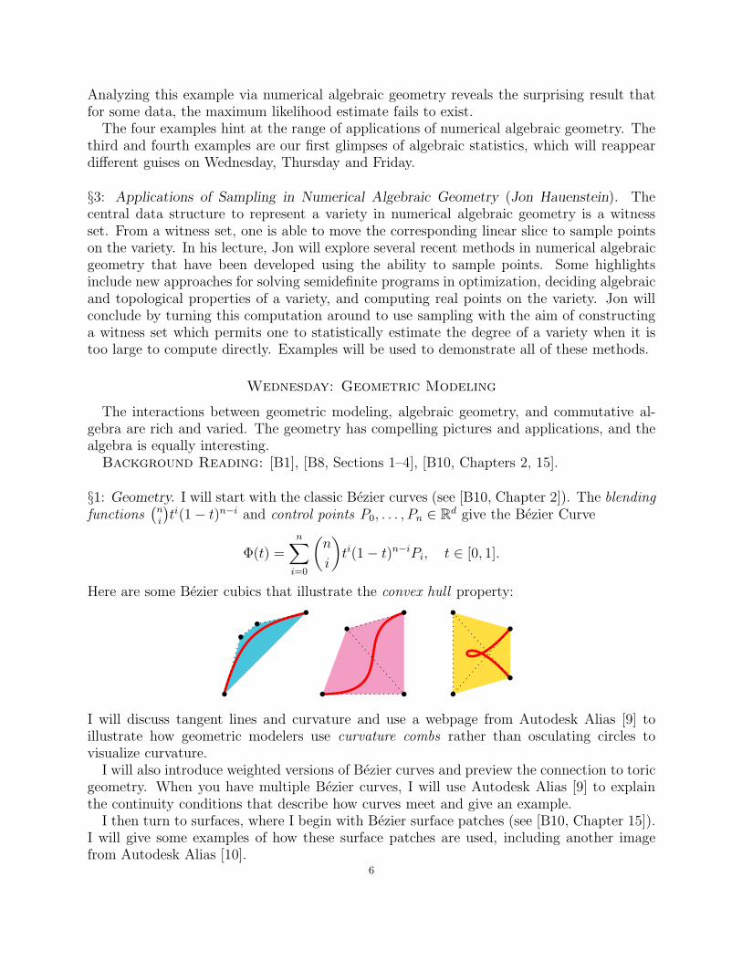
§1: Geometry. I will start with the classic Bezier curves (see [B10, Chapter 2]). The blendingfunctions

(n

i

)ti(1− t)n−i and control points P0, . . . , Pn ∈ Rd give the Bezier Curve

Φ(t) =n∑

i=0

(n

i

)

ti(1− t)n−iPi, t ∈ [0, 1].

Here are some Bezier cubics that illustrate the convex hull property:

I will discuss tangent lines and curvature and use a webpage from Autodesk Alias [9] toillustrate how geometric modelers use curvature combs rather than osculating circles tovisualize curvature.

I will also introduce weighted versions of Bezier curves and preview the connection to toricgeometry. When you have multiple Bezier curves, I will use Autodesk Alias [9] to explainthe continuity conditions that describe how curves meet and give an example.

I then turn to surfaces, where I begin with Bezier surface patches (see [B10, Chapter 15]).I will give some examples of how these surface patches are used, including another imagefrom Autodesk Alias [10].

6

In 2002, Krasauskas [78] defined toric patches, which include Bezier curves and surfaces.See [B8] for an introduction. A classic example due to Sottile [108] is

The data for a toric patch includes a weight assigned to each control point. By changingthe weights, one gets a family of toric patches that have interesting degenerations. I will usethis to explain the variation diminishing property of Bezier curves (Schoenberg 1930 [100])and also explain the image

due to Garcıa-Puente, Sottile and Zhu [47].The lecture will end with a discussion of the concept of linear precision. In the toric

context, this leads to rational linear precision, defined by Garcıa-Puente and Sottile in 2009[46]. I will give an example using a trapezoid and discuss a theorem from [46] that relatesrational linear precision to maximum likelihood estimates in algebraic statistics.

§2: Algebra. I will begin with plane curves and work projectively. From this point of view,a curve parametrization becomes a map ϕ : P1 → P2 whose image is a curve C ⊆ P2.After recalling the degree formula for ϕ, we turn to our first main topic, the implicitizationproblem, which seeks to find the defining equation of C, often called the implicit equation.One can use Grobner bases, as explained in [B3, Chapter 3] or in the recent work of Abbott,Bigatti and Robbiano [1].

However, we will instead focus on a different approach to implicitization that uses syzygies.If we write ϕ = (a, b, c), where a, b, c ∈ C[s, t] are relatively prime homogeneous polynomialsof degree n, then we get the ideal

I = 〈a, b, c〉 ⊆ R = C[s, t].

By the Hilbert Syzygy Theorem, I has a free resolution

0 −→ R(−n− µ1)⊕R(−n− µ2) −→ R(−n)3(a,b,c)−−−→ I −→ 0

with µ1 + µ2 = n. This was proved by Meyer in 1887 [89] and vastly generalized in 1890 byHilbert [65]. This exact sequence tells us that the syzygy module of I is free, with generatorsof degrees

µ = min(µ1, µ2) ≤ max(µ1, µ2) = n− µ.7

In geometric modeling, Sederberg, Anderson and Goldman used resultants to find theimplicit equation in 1984 [101]. In 1995, Sederberg and Chen [103] considered moving linesthat follow the parametrization. This led them to an equation of the form Aa+Bb+Cc = 0,which says that (A,B,C) is in the syzygy module of a, b, c.

This is where I got involved in geometric modeling. In 1998, Sederberg, Chen and Ipublished [34], which introduced the idea of a µ-basis. As I will explain, this gives a lovelygeometric way to think about syzygies and curve parametrizations. We will also see that theresultant of a µ-basis gives the implicit equation.

I will then turn to the Rees algebra, which for the ideal I ⊆ R is the graded R-algebraR(I) =

⊕∞

m=1 Imem ⊆ R[e]. Since I = 〈a, b, c〉, (x, y, z) 7→ (ae, be, ce) induces a surjection

R[x, y, z] → R(I). Generators of the kernel K are called defining equations of R(I).In 1997, Sederberg, Goldman, Du [102] generalized moving lines to moving curves that

follow the parametrization. These lie in the kernel K, which means that the geometricmodeling community independently discovered the defining equations of R(I) without anyidea of the connection to commutative algebra. The paper [102] also described minimalgenerators when a, b, c are generic of degree 4. I gave a rigorous proof of this in 2008 [32]. Inthe same year, Hoffman, Wang and I [33] found the defining equations for arbitrary n whenµ = 1. Many people have worked in the area, including Buse, Cortadellas, D’Andrea, Hong,Jia, Kustin, Madsen, Simis, Polini, Song, Vasconcelos, Ulrich and others.

Next come surfaces. The commutative algebra becomes more complicated, due in part tothe presence of basepoints, a new feature of the surface case. This complicates the degreeformula, which now involves the Hilbert-Samuel multiplicities of the basepoints.

In the affine case, one can show that the syzygy module is free of rank three. Geometrically,this gives moving planes p, q, r that give a basis of the syzygy module. However, there isno natural notion of minimal basis in the affine case, so that the resultant Res(p, q, r) hasan imperfect relation to the implicit equation of the parametrized surface—there may beextraneous factors, some coming from basepoints and some coming from ∞.

I will give an intuitive analysis of how basepoints affect Res(p, q, r), including an expla-nation of why it vanishes identically in the presence of a really bad basepoint. When thebasepoints are worst local almost complete intersections, Buse, Chardin and Jouanolou [27]showed in 2009 that

(1) Res(p, q, r) = F deg(ϕ) ×∏

ep>dp

Lep−dpp × extraneous factor from ∞

︸ ︷︷ ︸

described in [27]

,

where F = 0 is the implicit equation, Lp is a linear form, and ep−dp measures how farthe basepoint p is from being a local complete intersection. So there is clearly some lovelyalgebra and geometry going on here.

It is not easy to compute the moving planes p, q, r, and the extraneous factor at ∞ isannoying. A better approach is to use matrix representations, which are easy-to-constructmatrices that drop rank on the surface. As we learned on Monday, van der Waerden usedthis idea in 1926 [117] in his proof of the Fundamental Theorem of Elimination Theory.

In the situation here, again needs to worry about basepoints, and with the same hypothesis

as in (1), the paper [27] constructs a matrix that represents F deg(ϕ)×∏ep>dpLep−dpp . Although

the matrix is easy to describe, the proof uses the approximation complexes defined by Herzog,8

Simis and Vasconcelos in 1982 [64]. These complexes were first applied to geometric modelingand elimination theory in 2003 by Buse and Jouanolou [26].

When combined with numerical linear algebra, matrix representations lead to some niceapplications, such as the papers of Ba, Buse, Mourrain [12] on curve-surface intersections in2009 and Buse and Ba (2012) [25] on surface-surface intersections in 2012. I will concludeby revisiting the example from Botbol and Dickenstein [20] presented on Monday.

§3: Rees Algebras, Syzygies, and Computational Geometry (Hal Schenck). Rees and sym-metric algebras are fundamental topics in commutative algebra, and have recently enteredthe toolkit of computational geometers. In his lecture, Hal will begin with an overview ofthe basic machinery. Then he will introduce and develop some of the more specialized toolsused in the area, including Fitting ideals, the determinant of a complex, approximation com-plexes, and the McRae invariant. Hal will focus on applying these tools to several examplesof interest in geometric modeling.

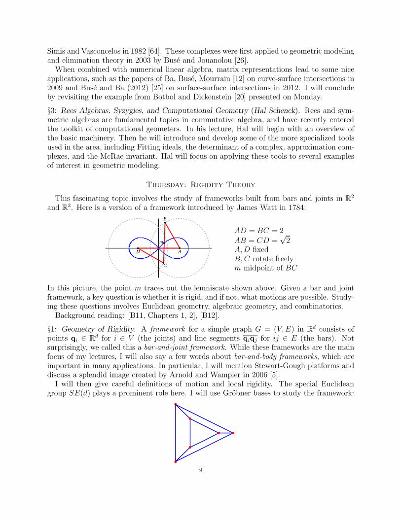
Thursday: Rigidity Theory

This fascinating topic involves the study of frameworks built from bars and joints in R2

and R3. Here is a version of a framework introduced by James Watt in 1784:

B

C

AD

m

AD = BC = 2

AB = CD =√2

A,D fixedB,C rotate freelym midpoint of BC

In this picture, the point m traces out the lemniscate shown above. Given a bar and jointframework, a key question is whether it is rigid, and if not, what motions are possible. Study-ing these questions involves Euclidean geometry, algebraic geometry, and combinatorics.

Background reading: [B11, Chapters 1, 2], [B12].

§1: Geometry of Rigidity. A framework for a simple graph G = (V,E) in Rd consists ofpoints qi ∈ Rd for i ∈ V (the joints) and line segments qiqj for ij ∈ E (the bars). Notsurprisingly, we called this a bar-and-joint framework. While these frameworks are the mainfocus of my lectures, I will also say a few words about bar-and-body frameworks, which areimportant in many applications. In particular, I will mention Stewart-Gough platforms anddiscuss a splendid image created by Arnold and Wampler in 2006 [5].

I will then give careful definitions of motion and local rigidity. The special Euclideangroup SE(d) plays a prominent role here. I will use Grobner bases to study the framework:

9

We will see that this framework is locally rigid but not infinitesimally rigid. I will alsomention a 1979 theorem of Asimow and Roth [8] which states that infinitesimal rigidityimplies local rigidity (so the converse fails by the above example).

Given a framework q ={qi

}

i∈Vin Rd for G = (V,E), one can define a rigidity matrix

RG,q which allows us to characterize infinitesimal rigidity in terms of the rank of RG,q. We

will use this to derive some inequalities that relate m = |E| to the number dn−(d+12

)(the

binomial coefficient is the dimension of SE(d)). I will then discuss various flavors of rigidity,which include local rigidity, infinitesimal rigidity, as well as global rigidity. And each of thesehave minimal and generic verisions.

For the remainder of the lecture, I take a more algebro-geometric point of view. If wefix the edge lengths, then all frameworks for G form a configuration variety in (Rd)n, wheren = |V |. Furthermore, this variety is smooth of dimension dn −m at frameworks q wherethe rigidity matrix RG,q has rank m = |E|.

As an application of these ideas, consider a 3-dimensional convex polytope P ⊆ R3. Itsedges give a graph G, and its vertices q ∈ (R3)n form a framework for G. I will prove a1978 theorem of Asimow and Roth [7] which states that q is locally rigid for G if and only ifevery face of P is a triangle. The proof uses a 1975 result of Gluck [54] and a classic resultof Cauchy whose proof is in THE BOOK [4].

I will conclude with Cayley-Menger varieties, which record the relations among the edgelengths of frameworks q ∈ (Rd)n for the complete graph Kn. Cayley determined theserelations in 1841 [29]. A change of variables relates this to variety of (n − 1) × (n − 1)symmetric matrices of rank ≤ d. The degree of this variety was determined in 1905 byGambelli [45], with rigorous proofs given in 1982 by Josefiak, Lascoux and Pragacz [69] andindependently in 1984 by Harris and Tu [60]. In 2004, Borcea and Streinu [19] used this toprove that if q has generic edge lengths, then up to congruence, the number of frameworksfor G with the same edge lengths as q is bounded by

n−d−2∏

ℓ=0

(n−1+ℓ

n−d−1−ℓ

)

(2ℓ+1ℓ

) .

I will also mention a 2018 paper by Capco, Gallet, Grasegger, Koutschan, Lubbes andSchicho [28] and a 2018 preprint by Bartzos, Emiris, Legersky and Tsigaridas [14].

§2: Combinatorics of Rigidity. I will begin with two examples of matroids : the linearlyindependents subsets of a finite set of vectors (a linear matroid) and the algebraically inde-pendent subsets of a finite set of elements in a field extension (an algebraic matroid). Withthese examples in mind, the definition of matroid in terms of independent sets follows easily.See [B11, Chapter 3] for more on matroids.

For us, a central object is the rigidity matroid Rd(n) of complete graph Kn in dimensiond. I will give two descriptions of Rd(n). The first is that Rd(n) is the linear matroid givenby the rows of the rigidity matrix RKn,q, where q ∈ (Rd)n is a suitably generic frameworkfor Kn.

The reason for using Kn is that is rows of RKn,q correspond to edges of Kn, so picking asubset E of rows gives a graph G(E) with edges E and vertices determined by the endpointsof E. Furthermore, if qE are the elements of q ∈ (Rd)n indexed by V (E), then rearranging

10

the columns of RKn,q gives

rows of RKn,q indexed by E =(RG(E),qE

| 0).

This allows us to relate local rigidity, infinitesimal ridigity and independence. For example,if |V (E)| ≥ d+ 1, then any two of the following imply the third:

• E is independent in Rd(n).• E is locally rigid.• |E| = d|V (E)| −

(d+12

).

I will then discuss a classic result proved by Gerard Laman [81] in 1970, which states thata generic framework in R2 for G is minimally locally rigid if and only if

|E| = 2|V | − 3 and |F | ≤ 2|V (F )| − 3 for all ∅ 6= F ⊆ E.

(Minimally locally rigid means that the framework is locally rigid but ceases to be so whenany edge is removed.) I will also mention the recent discovery of a 1927 paper by HildaPollaczek-Geiringer [96] that proves the same result.

This will be followed by a second description of the rigidity matroid Rd(n) as the algebraicmatroid of the Cayley-Menger variety defined in the previous lecture.

I will finish with an application of Rd(n) to algebraic statistics, following the 2018 paperThe maximum likelihood threshold of a graph by Gross and Sullivant [57]. After recallingthe Gaussian normal distribution, I will define a Gaussian graphical model N (0,Σ) on Rn,where the variables are indexed by the vertices of G = (V,E) and the model is determinedby a n× n symmetric positive definite matrix Σ with (Σ−1)ij = 0 for i 6= j and ij /∈ E.

A key question for a Gaussian graphical model is how many observations X(1), . . . , X(d) ∈Rn are needed in order to ensure the existence of a maximum likelihood estimate withprobability 1. It is straightforward to show that the MLE exists when d ≥ n.

A 2012 theorem of Uhler [115] gives the following sufficient condition for the existence ofthe MLE. If In,d ⊆ C[xij | 1 ≤ i ≤ j ≤ n] is the ideal defining the variety Symd(n) of n× nsymmetric matrices of rank ≤ d, then the MLE exists with probability 1 for G = (V,E) andd observations whenever

In,d ∩ C[xii, xij | i ∈ V, ij ∈ E] = {0}.This can be interpreted as saying that {xii, xij | i ∈ V, ij ∈ E} is an independent set in thealgebraic matroid of Symd(n) relative to the xij !

In the previous lecture, we noted a relation between symmetric matrices and Cayley-Menger varieties. This relation does not preserve the matroid structure, but in [57], Grossand Sullivant give a variant of this relation that leads to an isomorphism of matroids. Thisgives several interesting results. My favorite, which I will prove in detail, states that if G isa planar graph with n vertices, then the MLE of the Gaussian graphical model for G existsfor d ≥ 4 observations (with probability 1).

§3: Polynomial Methods and Rigidity Theory (Jessica Sidman). In combinatorial rigiditytheory, linearized constraint equations are used to study a generic framework associatedto a given graph G. In this setting, White and Whiteley defined a “pure condition,” apolynomial that vanishes for embeddings of G that are “special” or singular. In her lecture,Jessica will explain how this circle of ideas generalizes to other frameworks, including systemsof constraints that arise in common CAD software packages.

11

Returning to bar-and-joint frameworks, Jessica will contrast polynomial methods with thelinear-combinatorial ones. In particular, she will discuss rigidity of a framework in terms ofvarious algebraic matroids associated to it.

Friday: Chemical Reaction Neworks

A system of chemical or biochemical reactions gives a system of differential equations bythe law of mass action. These systems have a lovely structure whose analysis involves graphtheory and toric varieties.

Background reading: [B5, Sections 1, 2] and [B6, Lectures 1, 2].

§1: The Classical Theory of Chemical Reactions. The standard way of writing a chemicalreaction leads to a system of ODEs. An example involving nitrogen N and oxygen O is

(2) 2NO+ O2κ−−→ 2NO2

with reaction rate κ. Applying the law of mass action leads to the system of ODEs

(3)

d[NO]dt

= −2κ[NO]2[O2]d[O

2]

dt= −κ[NO]2[O2]

d[NO2]

dt= 2κ[NO]2[O2]

ord

dt

[NO][O2][NO2]

=

2 01 00 2

︸ ︷︷ ︸

Y

(− κ 0

κ 0

)

︸ ︷︷ ︸

Aκ

([NO]2[O2][N2O]2

)

︸ ︷︷ ︸

Φ

,

where [· · ·] denotes concentration, Φ consists of monomials in the concentrations comingfrom the law of mass action, Aκ is the transposed Laplacian of the weighted directed graph• κ→• underlying (2), and Y is the stoichiometric matrix that records the integer coefficientsappearing in (2). We also have species and complexes :

2NO + O2κ−−→ 2NO2

two complexes

three species

In this lecture, I will begin with the law of mass action (including its subtleties [58]) andthe general form of (3) for the vector of concentrations x, which following [B6] is given by

(4)dx

dt= Y AκΦ(x).

The steady states of such a system satisfy

(5) Y AκΦ(x) = 0.

For chemists and biologists, the steady states of interest are positive. Since reaction rates forindividual reactions are typically unknown, they are usually regarded as parameters, similarto the numerical polynomial systems discussed on Tuesday.

We often write a reaction network as a directed graph, such as

A + B κ12

#❍❍❍

❍c

κ21❍❍

❍❍

D

κ31 ;;✈✈✈✈C

κ23

oo

12

Note that the the vertices are the complexes. If the directed graph is G = (V,E), then thesystem (4) can be written

dx

dt=∑

i→j∈E

κi→jxyi (yj − yi), x = (x1, . . . , xn)

t,

where the yi are the columns of the stoichiometric matrix Y . This implies that solutions lieon translates of the stoichiometric subspace S = Span(yj − yi | i→j ∈ E). Intersecting thesetranslates with the positive orthant gives stoichiometric compatibility classes.

As a more substantial example of the biochemical reaction network, I will revisit theHIV model presented on Tuesday. I will then pose some general questions about steadystate solutions that involve multistationarity and whether solutions are locally or globallyattracting within their stoichiometric compatibility class. This is also a good time to mentionthe creators of this theory, Fritz Horn, Roy Jackson and Martin Feinberg. Among their manypapers are [44, 66, 67, 68].

I will conclude with complex balancing and the Deficiency Zero Theorem, proved by Hornin 1972 [66]. A network is complex balanced when it has a positive steady state solution x∗

of (5) that is a solution at the level of the complexes, i.e., AΦ(x∗) = 0, x∗ > 0. In 1972,Feinberg [44] defined the deficiency of a network to be

δ = m− ℓ− s,

where m = number of complexes, ℓ = number of connected components of the underlyinggraph, and s = dimension of the stoichiometric subspace S. The Deficiency Zero Theoremstates that a chemical reaction network is complex balanced for every set of positive reactionrates κ if and only if it has deficiency zero and is weakly reversible (meaning that everyconnected component of the underlying graph is strongly connected as a directed graph).

When the Deficiency Zero Theorem applies, the steady states are really nice:

• For any rate constants and any stoichiometric compatibility class, there is a unique

positive steady state solution x∗.• The solution x∗ is complex balanced and locally attracting.

The (still open) Global Attractor Conjecture asserts that x∗ is globally attracting.

§2: Toric Dynamical Systems. In 2009, Craicun, Dickenstein, Shiu and Sturmfels proposedthe name toric dynamical system for differential equations of the form (4) that have a positivecomplex balanced steady state solution, i.e., AκΨ(x∗) = 0, x∗ > 0. There are two mainreasons for the new name: the connection with toric varieties (more on this below) andthe fact that many systems of the form (4) have nothing to do with chemistry. I will giveexamples from epidemiology and population genetics.

I will then use the example

(6)

A+A

B +Bκ32−−−−−⇀↽−−−−−κ23

A+ B

κ 31

−−⇀↽−−κ 1

3

κ12

−−⇀↽−−κ21

to illustrate the Matrix Tree Theorem and show that we get a toric dynamical system if andonly if K1K3 = K2

2 , where13

K1 = κ21κ31 + κ23κ31 + κ32κ21

K2 = κ12κ32 + κ13κ32 + κ31κ12

K3 = κ13κ23 + κ12κ23 + κ21κ13.

It follows easily that (6) is a toric dynamical system when K1K3 = K22 , which defines a toric

variety when we use K1, K2, K3 as coordinates. We will see that this is no accident.I will then spend some time on the paper [37], defining toric ideals TG andMG and showing

how the latter leads algebraic equations generalizing K1K3 = K22 that characterize which

rate constants give a toric dynamical system. I will also explain how the codimension of thevariety defined by MG reveals the intrinsic meaning of the deficiency defined in the previouslecture. This will give an immediate proof of the Deficiency Zero Theorem!

The next portion of the lecture will be devoted to the work of Karin Gatermann, whosepapers [48, 49, 50, 51] published between 2001 and 2005 pioneered the use to toric methodsin the study of chemical reaction networks. I will quote part of Maurice Rojas’s Math Review[98] of one of her last papers before her tragic death in 2005.

To give of the flavor of what Gatermann did, I will follow a classic example

(7) Aκ12−−⇀↽−−κ21

2A A + Bκ34−−⇀↽−−κ43

Cκ45−−⇀↽−−κ54

B

due to Edelstein in 1970 [41]. Feinberg studied this example in his 1979 lectures [B6] andgave a nice picture to illustrate how multstationarity can occur:

x1

x2

x3

In 1989, Melenk, Moller and Neun [86] studied the steady states using Grobner basis methods,and this example also appears in Gatermann’s papers [49] (with Huber) and [50] (withWolfrum). To get a sense of the depth of Gatermann’s contributions, I will discuss thetreatment of (7) in [50]. For this example, Gatermann and Wolfrum introduce reaction

coordinates z1, . . . , z6 since (7) has six reactions. This leads to the deformed toric ideal

〈z4 − αz5, z2z6 − βz1z3〉 ⊆ Q(κ)[z1, . . . , z6], α =κ43

κ45, β =

κ21κ54

κ12κ34,

which has four Grobner bases corresponding to regular triangulations of the polytope P =Conv(y1, y2, y3, y4, y4, y5) (we think of these in terms of edges, so y4 gets repeated). Here

14

is one of the triangulations, which shows how each simplex picks four vertices that give asimpler reaction network:

z1 z2

z6 z3

z5

z1z2z3z5 :A −−⇀↽−− 2A

A + B −−→ C −−→ B

z1z3z5z6 :A −−→ 2A

A + B −−→ C −−⇀↽−− B

Geometrically, these simpler systems correspond to Grobner deformations. An importantobservation of [50] is that multistationarity in one of these simpler systems can persist tothe whole system. This idea underlies the recent research of Shiu and de Wolff [106] onclassifying small networks. I should also note that in (7), the complex C is an example of anintermediate. A recent paper by Sadeghimanesh and Feliu [99] explores how intermediatesinfluence the Grobner basis of the network.

This is all very rich material, but there is a further surprise in store, for the expression∑

i→j

κij︸︷︷︸

weights

xyi︸︷︷︸

blendingfunctions

(yj − yi)︸ ︷︷ ︸

controlpoints

has a natural interpretation in geometric modeling. In fact, Gheorges Craicun, one of theauthors of Toric Dynamical Systems [37], wrote a geometric modeling paper with Garcıa-Puente and Sottile [38] that relates Grobner deformations (such as above) to the toric degen-erations we saw on Wednesday. Craicun also wrote a paper with Feinberg [36] and postedan incomplete proof of the Global Attractor Conjecture in 2015 [35].

I will end by listing some further interesting topics about chemical reaction networks.

§3: Algebraic Methods for the Study of Biochemical Reaction Networks (Alicia Dickenstein).In recent years, techniques from computational and real algebraic geometry have been suc-cessfully used to address mathematical challenges in systems biology. The algebraic theoryof chemical reaction systems aims to understand their dynamic behavior by taking advan-tage of the inherent algebraic structure in the kinetic equations, and does not need a prioridetermination of the parameters, which can be theoretically or practically impossible.

In her lecture, Alicia will describe general results based on the network structure. In par-ticular, she will explain a general framework for biological systems, called MESSI systems,that describe Modifications of type Enzyme-Substrate or Swap with Intermediates, and in-clude many post-translational modification networks. Alicia will also outline recent methodsto address the important question of multistationarity.

Acknowledgements

I am very grateful to Doug Arnold, Dan Bates, Jon Hauenstein, Martin Kreuzer, KaieKubjas, Tom Sederberg, Jessica Sidman, Frank Sottile, Simon Telen, Caroline Uhler, andCharles Wampler for their assistance in preparing my lectures.

15

References

Background References

[B1] D. Cox, Curves, surfaces, and syzygies, in Topics in Algebraic Geometry and Geometric Modeling (R.Goldman and R. Krasauskas, eds.), Contemp. Math. 334, AMS, Providence, RI, 2003, 131–150.

[B2] D. Cox, What is a toric variety?, in Topics in Algebraic Geometry and Geometric Modeling (R.Goldman and R. Krasauskas, eds.), Contemp. Math. 334, AMS, Providence, RI, 2003, 203–223.

[B3] D. Cox, J. Little and D. O’Shea, Ideals, Varieties and Algorithms, Fourth Edition, Springer, NewYork, 2015.

[B4] D. Cox, J. Little and D. O’Shea, Using Algebraic Geometry, Second Edition, Springer, New York,2005.

[B5] A. Dickenstein, Biochemical reaction networks: An invitation for algebraic geometers, in MathematicalCongress of the Americas (J. de la Pea, J. A. Lopez-Mimbela, M. Nakamura and J. Petean, eds.),Contemp. Math. 656, AMS, Providence, RI, 2016, 65–83.

[B6] M. Feinberg, Lectures On Chemical Reaction Networks, 1979, https://crnt.osu.edu/

LecturesOnReactionNetworks.[B7] S. Hosten and S. Ruffa, Introductory notes to algebraic statistics, Rend. Istit. Mat. Univ. Trieste, Vol.

XXXVII (2005), 39–70.[B8] R. Krasauskas and R. Goldman, Toric Bezier patches with depth, in Topics in Algebraic Geometry and

Geometric Modeling (R. Goldman and R. Krasauskas, eds.), Contemp. Math. 334, AMS, Providence,RI, 2003, 65–91.

[B9] E. Penchevre, Justifying the ways of Etienne Bezout, 2016, arXiv:1606.03711[math.HO].[B10] T. Sederberg, Computer Aided Geometric Design, 2016, tom.cs.byu.edu/~557/text/cagd.pdf.[B11] B. Servatius, H. Servatius and J. Graver, Combinatorial Rigidity, AMS, Providence, RI, 1993.[B12] J. Sidman and A. St. John, The Rigidity of Frameworks: Theory and Applications, Notices of the

AMS, October 2017, 973–977.[B13] C. Wampler and A. Sommese, Numerical algebraic geometry and algebraic kinematics, Acta Numerica

20 (2011), 469–567.

References Mentioned in My Lectures

[1] J. Abbott, A. Bigatti and L. Robbiano, Implicitization of hypersurfaces, J. Symbolic Comput. 81(2017), 20–40.

[2] S. Abhyankar, Polynomials and power series, Math. Intelligencer 3, Springer-Verlag, September 1972.Reprinted in Algebra, Arithmetic and Geometry with Applications (C. Christensen, G. Sundaram, A.Sathaye and C. Bajaj, eds.), Springer, New York, 2004, 783–784.

[3] S. Abhyankar, Historical ramblings in algebraic geometry and related algebra, Amer. Math. Monthly83 (1976), 409–448.

[4] M. Aigner and G. Ziegler, Proofs from THE BOOK, Fifth Edition, Springer, New York, 2014.[5] D. Arnold and C. Wampler, poster image created for the IMA thematic year on IMA Applications of

Algebraic Geometry, https://www.ima.umn.edu/2006-2007.[6] B. Assarf, E. Gawrilow, K. Herr, M. Joswig, B. Lorenz, A. Paffenholz and T. Rehn, Computing convex

hulls and counting integer points with polymake, Math. Program. Comput. 9 (2017), 1–38.[7] L. Asimow and B. Roth, The rigidity of graphs, Trans. AMS 245 (1978), 279–289.[8] L. Asimow and B. Roth, The rigidity of graphs, II, J. Math. Anal. Appl. 68 (1979), 171–190.[9] Autodesk Alias Theory Builders, Evaluation 1: Curve Curvature, https://knowledge.autodesk.

com/support/alias-products/getting-started/caas/CloudHelp/cloudhelp/2016/ENU/Alias-

Tutorials/files/GUID-882B194B-E044-4921-B130-47391EFA1443-htm.html.[10] Autodesk Alias Theory Builders, Introduction to Continuity Terminology, https://knowledge.

autodesk.com/support/alias-products/getting-started/caas/CloudHelp/cloudhelp/2018/

ENU/Alias-Tutorials/files/GUID-E1BDFBD0-33CC-44C4-866D-5F367105A050-htm.html.

16

[11] W. Auzinger and H. Stetter, An elimination algorithm for the computation of all zeros of a system ofmultivariate polynomial equations, in Numerical Mathematics Singapore 1988 (R. Agarwal, Y. Chowand S. Wilson, eds.) International Series of Numerical Mathematics 86, Birkhuser, Basel, 1988, 11–30.

[12] L. Ba, L. Buse and B. Mourrain, Curve/surface intersection problems by means of matrix represen-tations, in Proceedings of the 2009 conference on Symbolic Numeric Computation (H. Kai and H.Sekigawa, eds.), ACM, New York, 2009, 71–78.

[13] C. Baciu and M. Kreuzer, Algebraisches Ol, Mitteilungen der DMV 19 (2011), 142–147.[14] E. Bartzos, I. Emiris, J. Legersky and E. Tsigaridas, On the maximal number of real embeddings of

spatial minimally rigid graphs, 2018, arXiv:1802.05860[math.AG].[15] D. Bates, J. Hauenstein, A. Sommese and C. Wampler, Numerically Solving Polynomial Systems with

Bertini, SIAM, Philadelphia, PA, 2013.[16] D. Bates, J. Hauenstein, A. Sommese and C. Wampler, Bertini: Software for Numerical Algebraic

Geometry, https://bertini.nd.edu.[17] E. Bezout, Sur le degre des equations resultantes de l’evanouissement des inconnues, Histoire de

l’Acadmie Royale des Sciences (1764), 288–338.[18] E. Bezout, Theorie generale des equations algebriques, Ph.-D. Pierres, Paris, 1779. English translation

General Theory of Algebraic Equations by Eric Feron, Princeton Univ. Press, Princeton, NJ, 2006.[19] C. Borcea and I. Streinu, On the number of embeddings of minimally rigid graphs, Discrete Comput.

Geom. 31 (2004), 287–303.[20] N. Botbol and A. Dickenstein, Implicitization of rational hypersurfaces via linear syzygies: a practical

overview, J. Symbolic Comput. 74 (2016), 493–512.[21] O. Bonnet, Memoire sur la resolution de deux equations a deux inconnues, Nouvelles Annales de

Mathematiques 6 (1847), 54–63, 135–150, 243–252.[22] A. Brill, Ueber eine Eigenschaft der Resultante, Math. Annalen 16 (1880), 345–347.[23] B. Buchberger, Ein Algorithmus zum Auffinden der Basiselemente des Restklassenringes nach einem

nulldimensionalen Polynomideal, Ph.D. Thesis, University of Innsbruck, 1965.[24] B. Buchberger, Ein algorithmisches Kriterium fur die Losbarkeit eines algebraischen Gleichungssys-

tems, Aequationes mathematicae 4, 374–383.[25] L. Buse and T. Ba, The surface/surface intersection problem by means of matrix based representations,

Comput. Aided Geom. Des. 29 (2012), 579–598.[26] L. Buse and J.-P. Jouanolou, On the closed image of a rational map and the implicitization problem,

J. Algebra 265 (2003), 312–357.[27] L. Buse, M. Chardin and J.-P. Jouanolou, Torsion of the symmetric algebra and implicitization, Proc.

Amer. Math. Soc. 137 (2009), 1855–1865.[28] J. Capco, M. Gallet, G. Grasegger, C. Koutschan, N. Lubbes and J. Schicho, The number of realizations

of a Laman graph, SIAM J. Appl. Algebra Geom. 2 (2018), 94–125.[29] A. Cayley, A theorem in the geometry of position, Cambridge Mathematical Journal 2 (1841), 267–271.[30] A. Cayley, Nouvelles recherches sur l’elimination et la theorie des courbes, J. Reine Angew. Math. 63

(1864), 34–39.[31] T. Chen, T. Lee and T. Li, Hom4PS-3: A parallel numerical solver for systems of polynomial equations

based on polyhedral homotopy continuation methods, in Mathematical Software – ICMS 2014 (H. Hongand C. Yap, eds.), Lecture Notes in Computer Science 8592. Springer, Berlin, 2014, 183–190.

[32] D. Cox, The moving curve ideal and the Rees algebra, Theoret. Comput. Sci. 28 (2008), 23–36.[33] D. Cox, J. Hoffman and H. Wang, Syzygies and the Rees algebra, J. Pure Appl. Algebra 212 (2008),

1787–1796.[34] D. Cox, T. Sederberg and F. Chen, The moving line ideal basis of planar rational curves, Comput.

Aided Geom. Des. 15 (1998), 803–827.[35] G. Craciun, Toric differential inclusions and a proof of the global attractor conjecture, 2015, arXiv:

1501.02860[math.DS].[36] G. Craciun and M. Feinberg, Multiple equilibria in complex chemical reaction networks: semiopen mass

action systems, SIAM J. Appl. Math. 70 (2010), 1859–1877.[37] G. Craciun, A. Dickenstein, A. Shiu and B. Sturmfels, Toric dynamical systems, J. Symbolic Comput.

44 (2009), 1551–1565.

17

[38] G. Craciun, L. Garcia-Puente and F. Sottile, Some geometrical aspects of control points for toricpatches, in Mathematical methods for curves and surfaces (M. Dæhlen, M. Floater, T. Lyche, J.-L.Merrien, K. Mørken and L. Schumaker, eds.), Lecture Notes in Comput. Sci. 5862, Springer, Berlin,2010, 111–135.

[39] G. Cramer, Introduction a l’analyse des lignes courbes algebriques, Freres Cramer et Cl. Philibert,Geneve, 1750.

[40] A. Dixon, The eliminant of three quantics in two independent variables, Proc. London Math. Soc. 7(1909), 46–49, 473–492.

[41] B. Edelstein, Biochemical models with multiple steady states and hysteresis, J. Theor. Biol. 29 (1970),57–62.

[42] F. Enriques and O. Chisini, Lezione sulla teoria geometrica delle equazioni e delle funzioni algebriche,Volume 1, Nicola Zanichelli, Bologna, 1915.

[43] I. Faux and M. Pratt, Computational Geometry for Design and Manufacture, Ellis Horwood, Chich-ester, 1979.

[44] M. Feinberg, Complex balancing in general kinetic systems, Arch. Rational Mech. Anal. 49 (1972),187–194.

[45] G. Giambelli, Sulle varieta rappresentate coll’annullare determinanti minori contenuti in un determi-nante simmetrico od emisimmetrico generico di forme, Atti R. Accad. Sci. Torino 44 (1905/1906),102–125.

[46] L. Garcıa-Puente and F. Sottile, Linear precision for parametric patches, Adv. Comput. Math. 33(2010), 191–214.

[47] L. Garcıa-Puente, F. Sottile and C. Zhu, Toric degenerations of Bezier patches, ACM Transactions onGraphics 30 (2011), 110:1–110:10.

[48] K. Gatermann, Counting stable solutions of sparse polynomial systems in chemistry, in Symbolic Com-putation: Solving Equations in Algebra, Geometry and Engineering (E. Green, S. Hosten, R. Lauben-bacher and V. Powers, eds.), Contemporary Mathematics 286, AMS, Providence, RI, 2001, 53–69.

[49] K. Gatermann and B. Huber, A family of sparse polynomial systems arising in chemical reactionsystems, J. Symbolic Comput. 33 (2002), 275–305.

[50] K. Gatermann and M. Wolfrum, Bernstein’s second theorem and Viro’s method for sparse polynomialsystems in chemistry, Adv. in Appl. Math. 34 (2005), 252–294.

[51] K. Gatermann, M. Eiswirth and A. Sensse, Toric ideals and graph theory to analyze Hopf bifurcationsin mass action systems, J. Symbolic Comput. 40 (2005), 1361–1382.

[52] I. Gel’fand, M. Kapranov and A. Zelevinsky, Discriminants, Resultants, and Multidimensional Deter-minants, Birkhauser, Boston, 1994.

[53] J. Giraud, Geometrie algebrique elementaire, Cours de troisieme cycle (1975-76), Publ. Math. D’Orsay,No 77-75, Orsay, 1977.

[54] H. Gluck, Almost all simply connected closed surfaces are rigid, in Geometric Topology (L. Glaser andT. Rushing, eds.), Lecture Notes in Math. 438, Springer-Verlag, Berlin, 1975, 225–239.

[55] D. Grayson and M. Stillman, Macaulay2, a software system for research in algebraic geometry, http://www.math.uiuc.edu/Macaulay2/.

[56] E. Gross, B. Davis, K. Ho, D. Bates, and H. Harrington, Numerical algebraic geometry for modelselection and its application to the life sciences, J. R. Soc. Interface 13 (2016), 20160256.

[57] E. Gross and S. Sullivant, The maximum likelihood threshold of a graph, Bernoulli 24 (2018), 386–407.[58] J. Gunawardena, Theory and Mathematical Methods, Comprehensive Biophysics 9 (2012), 243–265.[59] J. Harris, Galois groups of enumerative problems, Duke Math. J. 46 (1979), 685–724.[60] J. Harris and L. Tu, On symmetric and skew-symmetric determinantal varieties, Topology 23 (1984),

71–84.[61] V. Hars and J. Toth, On the inverse problem of reaction kinetics, in Qualitative Theory of Differential

Equations (M. Farkas, ed.), Colloquia Mathematica Societatis Janos Bolyai 30, North-Holland Publ.Co., Amsterdam, 1981, 363–379.

[62] R. Hartshorne, Algebraic Geometry, Springer, 1978.[63] D. Heldt, M. Kreuzer, S. Pokutta and H. Poulisse, Approximate computation of zero-dimensional

polynomial ideals, J. Symbolic Comput. 44 (2009), 1566–1591.

18

[64] J. Herzog, A. Simis and W. Vasconcelos, Approximation complexes of blowing-up rings, J. Algebra 74

(1982), 466–493.[65] D. Hilbert, Ueber die Theorie der algebraischen Formen, Math. Annalen 36 (1890), 473–534.[66] F. Horn, Necessary and sufficient conditions for complex balancing in chemical kinetics, Arch. Ration.

Mech. Anal. 49 (1972), 172–186.[67] F. Horn, The dynamics of open reaction systems, inMathematical Aspects of Chemical and Biochemical

Problems and Quantum Chemistry (Proc. SIAM-AMS Sympos. Appl. Math., New York) (D. Cohen,ed.), SIAM-AMS Proceedings 8, AMS, Providence, R.I., 1974, 125–137.

[68] F. Horn and R. Jackson, General mass action kinetics, Arch. Ration. Mech. Anal. 47 (1972), 81–116.[69] T. Jozefiak, A. Lascoux and P. Pragacz, Classes of determinantal varieties associated with symmetric

and antisymmetric matrices, in Proceedings of the Week of Algebraic Geometry (Bucharest, 1980) (L.Badescu and H. Kurke eds.), Teubner-Texte zur Math. 40, Teubner, Leipzig, 1981, 106–108.

[70] J.-P. Jouanolou, Singularites rationnelles du resultant, in Algebraic Geometry, Proceedings Copenhagen1978 (K. Lønsted, ed.), Lecture Notes in Math. 732, Springer, New York, 1979, 183–213.

[71] J.-P. Jouanolou, Ideaux resultants, Adv. Math. 37 (1980), 212–238.[72] J.-P. Jouanolou, Le formalisme du resultant, Adv. Math. 90 (1991), 117–263.[73] J.-P. Jouanolou, Aspects invariants de l’elimination, Adv. Math. 114 (1995), 1–174.[74] J.-P. Jouanolou, Resultant anisotrope, complements et applications, Electron. J. Combin. 3 (1996),

no. 2, Research Paper 2.[75] J.-P. Jouanolou, Formes d’inertie et resultant: un formulaire, Adv. Math. 126 (1997), 119–250.[76] S. Kleiman, Bertini and his two fundamental theorems, Rend. Circ. Mat. Palermo (2) Suppl. 55 (1998),

9–37.[77] D. Kosta and K. Kubjas, Geometry of symmetric group-based models, 2017, arXiv:1705.09228[q-

bio.PE].[78] R. Krasauskas, Toric surface patches, Adv. Comput. Math. 17 (2002), 89–113.[79] M. Kreuzer, H. Poulisse and L. Robbiano, From oil fields to Hilbert schemes, in Approximate Com-

mutative Algebra (L. Robbiano and J. Abbott, eds.), Springer-Verlag, Vienna, 2010, 1–54.[80] L. Kronecker, Grundzuge einer arithmetischen Theorie der algebraischen Grossen, J. Reine Angew.

Math. 92 (1882), 1–122.[81] G. Laman, On graphs and the rigidity of plane skeletal structures, J. Engineering Mathematics 4

(1970), 331–340.[82] D. Lazard, Algebre lineaire sur K[X1, · · · , Xn], et elimination, Bull. Soc. Math. France 105 (1977),

165–190.[83] A. Leykin, Numerical algebraic geometry, J. Softw. Algebra Geom. 3 (2011), 5–10.[84] F. Macaulay, On some Formulæ in Elimination, Proc. London Math. Soc. 35 (1903) 3–27,[85] F. Macaulay, The Algebraic Theory of Modular Systems, Cambridge Univ. Press, Cambridge, 1916.[86] H. Melenk, H. Moller and W. Neun, Symbolic solution of large stationary chemical kinetics problems,

Impact of Computing in Science and Engineering 1 (1989), 138–167.

[87] F. Mertens, Uber die bestimmenden Eigenschaften der Resultante von n Formen mit n Veranderlichen,Sitzungsberichte der Mathematisch-Naturwissenschaftlichen Classe der Kaiserlichen Akademie derWissenschaften, II. Abtheilung 93 (1886), 527–566.

[88] F. Mertens, Zur Theorie der Elimination, Teil II, Sitzungsber. Akad. Wien 108 (1899), 1344–1386.[89] F. Meyer, Zur Theorie der reducibeln ganzen Functionen von n Variabeln, Math. Annalen 30 (1887),

30–74.[90] F. Minding, Ueber die Bestimmung des Grades einer durch Elimination hervorgehenden Gleichung,

J. Reine Angew. Math. 22 (1841), 178–183. English translation with commentary by David Coxand Maurice Rojas in Topics in Algebraic Geometry and Geometric Modeling (R. Goldman and R.Krasauskas, eds.), Contemp. Math. 334, AMS, Providence, RI, 2003, 351–362.

[91] E. Netto, Vorlesungen uber Algebra, Volume II, Teubner, Leipzig, 1900.[92] E. Netto and R. Le Vavasseur, Fonctions rationalles, in Encyclopedie des sciences mathematiques pures

et appliquees Tome I, Volume 2 (J. Molk, ed.), Gauthiers-Villars, Paris and B. G. Teubner, Leipzig,1909, 1–232.

19

[93] I. Newton, The Mathematical Papers of Isaac Newton, Volume II, (D. T. Whiteside, ed.) CambridgeUniv. Press, Cambridge, 1972, p. 177.

[94] E. Penchevre, Histoire de la theorie de l’elimination, Ph.D. Thesis, l’Universite Paris VII, 2006.

[95] S.-D. Poisson, Memoire sur l’elimination dans les equations algebriques, J. Ec. polytech. Math. 4(1802), 199–203.

[96] H. Pollaczek-Geiringer, Uber die Gliederung ebener Fachwerke, Z. Angew. Math. Mech. 7 (1927),58–72.

[97] B. Riemann, Theorie der Abel’schen Functionen, J. Reine Angew. Math. 54 (1857), 101–155.[98] M. Rojas, Review of [51], Mathematical Reviews, MR2178092 (2006m:13026).[99] A. Sadeghimanesh and E. Feliu, Grobner bases of reaction networks with intermediate species, 2018,

arXiv:1804.01381[cs.SC]

[100] L. Schoenberg, Uber variationsvermindernde lineare Transformationen, Math. Z. 32 (1930), 321–328.[101] T. Sederberg, D. Anderson and R. Goldman, Implicit representation of parametric curves and surfaces,

Comput. Vision Graphics Image Process. 28 (1984), 72–84.[102] T. Sederberg, R. Goldman and H. Du, Implicitizing rational curves by the method of moving algebraic

curves, J. Symbolic Comput. 23 (1997), 153–175.[103] T. Sederberg and F. Chen, Implicitization using moving curves and surfaces, in SIGGRAPH 95 Pro-

ceedings (R. Cook, ed.), ACM, New York, 1995, 301–308.[104] T. Sederberg, T. Saito, D. Qi and K. Klimaszewksi, Curve implicitization using moving lines, Comput.

Aided Geom. Design 11 (1994), 687–706.[105] F. Severi, Sul principio della conservazione del numero, Rend. Circ. Mat. Palermo 33 (1912), 313-327.[106] A. Shiu and T. de Wolff, Nondegenerate multistationarity in small reaction networks, 2018, arXiv:

1802.00306[math.DS].[107] A. Sommese and C. Wampler, The Numerical Solution of Systems of Polynomials: Arising in Engi-

neering And Science, World Scientific Pub Co., Hackensack, New Jersey, 2005.[108] F. Sottile, Toric ideals, real toric varieties, and the moment map, in Topics in Algebraic Geometry and

Geometric Modeling (R. Goldman and R. Krasauskas, eds.), Contemp. Math. 334, AMS, Providence,RI, 2003, 225–240.

[109] G. Stagliano, A package for computations with classical resultants, 2017, arXiv:1705.01430[math.AG].

[110] H. Stetter, Numerical Polynomial Algebra, SIAM, Philadelphia, PA, 2004.[111] J. Sylvester, A Method of determining by mere Inspection the derivatives from two Equations of any

degree, Philos. Mag. XVI (1840), 132-135.[112] S. Telen and M. Van Barel, A stabilized normal form algorithm for generic systems of polynomial

equations, 2017, arXiv:1708.07670[math.NA].[113] W. Trinks, Uber B. Buchbergers Verfahren, Systeme algebraischer Gleichungen zu losen, J. Number

Theory 10 (1978), 475–488.[114] E. Tschirnhaus, Methodus auferendi omnes terminos intermedios ex data equatione, Acta Eruditorium

2 (1683), 204–207.[115] C. Uhler, Geometry of maximum likelihood estimation in Gaussian graphical models, Ann. Statist. 40

(2012), 238–261.[116] B. van der Waerden, Zur Nullstellentheorie der Polynomideale, Math. Annalen 96 (1926), 183–208.[117] B. van der Waerden, Ein algebraisches Kriterium fur die Losbarkeit von homogenen Gleichungen,

Nederl. Akad. Wetensch. Proc. 29 (1926), 142–149.[118] B. van der Waerden, Der Multiplizitatsbegriff der algebraischen Geometrie, Math. Annalen 97 (1927),

756–774.[119] B. van der Waerden, The foundation of algebraic geometry from Severi to Andre Weil, in Actes du

Congres International des Mathematiciens 1970, Volume 3, Gauthier-Villars, Paris, 1971.[120] C. van Loan, Introduction to Scientific Computing: A Matrix-Vector Approach Using MATLAB, second

edition, Pearson, Upper Saddle River, NJ, 2000.[121] C. Wampler, A. Morgan and A. Sommese, Complete solution of the nine-point path synthesis problem

for four-bar linkages, J. Mech. Des. 114 (1992), 153–159.

20

[122] E. Waring,Meditationes Algebraicæ, Third Edition, J. Nicholson, Cambridge, 1782. English translationby Dennis Weeks, AMS, Providence, RI, 1991.

[123] A. Weil, Foundations of Algebraic Geometry, AMS, Providence, RI, 1946.[124] J. Verschelde, Algorithm 795: PHCpack: A general-purpose solver for polynomial systems by homotopy

continuation, ACM Trans. Math. Software 25 (1999), 251–276.[125] Wolfram Research, Inc., Mathematica, Version 10.1, Champaign, IL, 2015.

21